Hartle-Hawking wavefunction in double scaled SYK

Abstract

We compute the transition amplitude between the chord number $0$ and $\ell$ states in the double scaled SYK model and interpret it as a Hartle-Hawking wavefunction of the bulk gravitational theory. We observe that the so-called un-crossed matter correlators of double scaled SYK model are obtained by gluing the Hartle-Hawking wavefunctions with an appropriate weight.

1 Introduction

Sachdev-Ye-Kitaev (SYK) model kitaev1 ; kitaev2 ; Sachdev1993 ; Maldacena:2016hyu ; Polchinski:2016xgd is a useful toy model for the study of quantum gravity. The low energy sector of SYK model is described by the Schwarzian mode and this part of the dynamics is holographically dual to Jackiw-Teitelboim (JT) gravity Jackiw:1984je ; Teitelboim:1983ux . As discussed in Cotler:2016fpe ; Berkooz:2018qkz ; Berkooz:2018jqr , one can go beyond this low energy approximation by taking a certain double scaling limit of the SYK model. It turns out that this double scaled SYK (DSSYK) model is exactly solvable using the technique of the chord diagram Berkooz:2018qkz ; Berkooz:2018jqr . However, as emphasized in Lin:2022rbf , the bulk gravitational picture of DSSYK is not well understood. One mysterious feature of DSSYK is that the geodesic length of bulk spacetime becomes a discrete chord number $\ell$. It is proposed in Lin:2022rbf that the chord number state $|\ell\rangle$ originally introduced in Berkooz:2018jqr should be identified as the state of bulk Hilbert space and the expression of the partition function $Z(\beta)=\langle 0|e^{-\beta T}|0\rangle$ in terms of the transfer matrix $T$ acting on the chord number states has a natural bulk gravitational interpretation.

Generalizing this interpretation in Lin:2022rbf , we propose that the amplitude $\langle\ell|e^{-\beta T}|0\rangle$ is interpreted as the Hartle-Hawking (HH) wavefunction of the bulk gravitational theory Hartle:1983ai and we explicitly compute $\langle\ell|e^{-\beta T}|0\rangle$. We realize that the HH wavefunction has been secretly appeared in appendix C of Berkooz:2018jqr in the computation of the so-called un-crossed matter correlators in DSSYK. Thus we find a bulk gravitational interpretation of the un-crossed correlators: these correlators are obtained by gluing the HH wavefunctions with an appropriate weight.

This paper is organized as follows. In section 2, we review the solution of DSSYK in terms of the chord diagrams and the transfer matrix Berkooz:2018jqr . In section 3, we compute the HH wavefunction $\langle\ell|e^{-\beta T}|0\rangle$. In section 4, we present our observation that the un-crossed correlators in appendix C of Berkooz:2018jqr are written in terms of the HH wavefunctions. In section 5, we consider the probability distribution of chord number $\ell$ given by the absolute value squared $|\langle\ell|e^{-\beta T}|0\rangle|^{2}$ of the HH wavefunction. Finally we conclude in section 6 with some discussion on the future problems.

2 Review of doubled scaled SYK

We first review the result of DSSYK in Berkooz:2018jqr . SYK model is defined by the Hamiltonian for $N$ Majorana fermions $\psi_{i}~{}(i=1,\cdots,N)$ with all-to-all $p$-body interaction

$$H=\mathrm{i}^{p/2}\sum_{i_{1},\cdots,i_{p}=1}^{N}J_{i_{1}\cdots i_{p}}\psi_{i_{1}}\cdots\psi_{i_{p}},$$ (1)

where $\psi_{i}$’s obey the anti-commutation relation $\{\psi_{i},\psi_{j}\}=2\delta_{i,j}$ and the random coupling $J_{i_{1}\cdots i_{p}}$ is drawn from the Gaussian distribution

$$\langle J_{i_{1}\cdots i_{p}}\rangle_{J}=0,\quad\langle J_{i_{1}\cdots i_{p}}^{2}\rangle_{J}=\binom{N}{p}^{-1}.$$ (2)

DSSYK is defined by the limit

$$N,p\to\infty\quad\text{with}\quad\lambda=\frac{2p^{2}}{N}:\text{fixed}.$$ (3)

As shown in Berkooz:2018jqr , SYK model is exactly solvable in this double scaling limit. In the computation of the trace $\langle\operatorname{tr}H^{k}\rangle_{J}$, the average over the random coupling $J$ can be organized as the so-called chord diagram arising from the Wick contraction of $J$’s and the remaining trace of Majorana fermions reduces to a counting problem of the intersection number of chords

$$\langle\operatorname{tr}H^{k}\rangle_{J}=\sum_{\text{chord diagrams}}q^{\#(\text{intersections})},$$ (4)

where $q$ is given by

$$q=e^{-\lambda}.$$ (5)

This counting problem is solved by introducing the transfer matrix acting on the states $\{|n\rangle\}_{n=0,1,\cdots}$. Here $|n\rangle$ denotes the state with $n$ chords

(6)

and the dashed line in (6) represents a constant (Euclidean) time slice. We normalize $|n\rangle$ as

$$\langle n|m\rangle=\delta_{n,m},\quad 1=\sum_{n=0}^{\infty}|n\rangle\langle n|.$$ (7)

Then the partition function $Z(\beta)$ of DSSYK is written as

$$Z(\beta)=\langle\operatorname{tr}e^{-\beta H}\rangle_{J}=\langle 0|e^{-\beta T}|0\rangle,$$ (8)

where the transfer matrix $T$ is written in terms of the $q$-deformed oscillator $A_{\pm}$ as

$$-T=A_{-}+A_{+}.$$ (9)

$A_{\pm}$ acts on the state $|n\rangle$ as

$$A_{-}|n\rangle=\sqrt{[n]}|n-1\rangle,\quad A_{+}|n\rangle=\sqrt{[n+1]}|n+1\rangle,$$ (10)

where $[n]$ is the $q$-integer

$${[}n{]}=\frac{1-q^{n}}{1-q}.$$ (11)

From (10), one can easily show that $A_{\pm}$ obey the relations

$$A_{-}A_{+}-qA_{+}A_{-}=1,\quad[A_{-},A_{+}]=q^{\widehat{N}},$$ (12)

where $\widehat{N}$ is the number operator

$$\widehat{N}|n\rangle=n|n\rangle.$$ (13)

Some comments are in order here:

1. Our $-T$ in (9) is equal to $\hat{T}$ in Berkooz:2018jqr , which is related to the original $T$ in Berkooz:2018jqr by a conjugation. Put differently, the original $T$ in Berkooz:2018jqr is obtained from our $-T$ in (9) by acting it on a different basis $\{A_{+}^{n}|0\rangle\}_{n=0,1,\cdots}$

   $$-TA_{+}^{n}|0\rangle=A_{+}^{n+1}|0\rangle+\frac{1-q^{n}}{1-q}A_{+}^{n-1}|0\rangle,$$ (14)

   where $-T=A_{-}+A_{+}$ in (9). Note that the state $A_{+}^{n}|0\rangle$ is related to $|n\rangle$ as

   $$A_{+}^{n}|0\rangle=\sqrt{[n]!}|n\rangle,\qquad[n]!=\prod_{k=1}^{n}[k],$$ (15)

   and the norm of $A_{+}^{n}|0\rangle$ is given by the $q$-factorial of $n$

   $$\big{|}A_{+}^{n}|0\rangle\big{|}^{2}=[n]!.$$ (16)

   This basis and normalization were adopted in Lin:2022rbf .

2. We have put the minus sign in the definition of $T$ in (9). This minus sign does not change the final result since the spectrum of the Hamiltonian is symmetric under the sign flip $H\to-H$. This symmetry can be traced back to the Gaussian distribution of the random coupling $J$, where $+J$ and $-J$ appear with an equal probability.

As shown in Berkooz:2018jqr , one can compute the partition function in (8) by going to the eigenbasis of the transfer matrix $T$, which is given by the $q$-Hermite polynomial $H_{n}(\cos\theta|q)$

$$\langle\theta|n\rangle=\frac{H_{n}(\cos\theta|q)}{\sqrt{(q;q)_{n}}},$$ (17)

where $(a;q)_{n}$ denotes the $q$-Pochhammer symbol

$$(a;q)_{n}=\prod_{k=0}^{n-1}(1-aq^{k}),$$ (18)

and the $q$-Hermite polynomial is defined by

$$H_{n}(\cos\theta|q)=\sum_{k=0}^{n}\Bigl{[}~{}\begin{matrix}n\\ k\end{matrix}~{}\Bigr{]}_{q}e^{\mathrm{i}(n-2k)\theta},$$ (19)

with $\Bigl{[}~{}\begin{matrix}n\\ k\end{matrix}~{}\Bigr{]}_{q}$ being the $q$-binomial coefficient

$$\Bigl{[}~{}\begin{matrix}n\\ k\end{matrix}~{}\Bigr{]}_{q}=\frac{(q;q)_{n}}{(q;q)_{k}(q;q)_{n-k}}.$$ (20)

Using the recurrence relation for the $q$-Hermite polynomial, one can show that $T$ is diagonal in this basis

$$\langle\theta|T|n\rangle=E(\theta)\langle\theta|n\rangle,$$ (21)

and the eigenvalue $E(\theta)$ is given by

$$E(\theta)=-\frac{2\cos\theta}{\sqrt{1-q}}.$$ (22)

$\langle\theta|n\rangle$ obeys an orthogonality relation with respect to a certain integration measure of $\theta$

$$\int_{0}^{\pi}\frac{d\theta}{2\pi}\mu(\theta)\langle n|\theta\rangle\langle\theta|m\rangle=\delta_{n,m},$$ (23)

where the measure factor $\mu(\theta)$ is given by

$$\mu(\theta)=(q;q)_{\infty}(e^{2\mathrm{i}\theta};q)_{\infty}(e^{-2\mathrm{i}\theta};q)_{\infty}.$$ (24)

Then the partition function (8) is written as

$$\langle 0|e^{-\beta T}|0\rangle =\int_{0}^{\pi}\frac{d\theta}{2\pi}\mu(\theta)\langle 0|\theta\rangle e^{-\beta E(\theta)}\langle\theta|0\rangle$$ (25)

$$=\int_{0}^{\pi}\frac{d\theta}{2\pi}\mu(\theta)e^{-\beta E(\theta)},$$

where we used $\langle\theta|0\rangle=\frac{H_{0}(\cos\theta|q)}{\sqrt{(q;q)_{0}}}=1$. This integral was evaluated in Berkooz:2018jqr as

$$\langle 0|e^{-\beta T}|0\rangle=\sum_{r=0}^{\infty}(-1)^{r}q^{\frac{1}{2}r(r+1)}(2r+1)\frac{\sqrt{1-q}}{\beta}I_{2r+1}\left(\frac{2\beta}{\sqrt{1-q}}\right),$$ (26)

where $I_{n}(z)$ denotes the modified Bessel function of the first kind. In the next section, we will compute the more general amplitude of $e^{-\beta T}$ sandwiched between $n=0$ and $n=\ell$

$$\langle\ell|e^{-\beta T}|0\rangle,$$ (27)

which we interpret as the Hartle-Hawking (HH) wavefunction of the bulk gravitational theory.

3 Hartle-Hawking wavefunction in doubled scaled SYK

Let us consider the amplitude $\langle\ell|e^{-\beta T}|0\rangle$ in (27). In the bulk gravitational picture, it is suggested in Berkooz:2018qkz ; Berkooz:2018jqr ; Lin:2022rbf that the chord number $\ell$ in $|\ell\rangle$ can be interpreted as the discretized version of the geodesic length of the bulk spacetime. The bulk picture of the amplitude $\langle\ell|e^{-\beta T}|0\rangle$ is depicted as

(28)

which is naturally interpreted as the HH wavefunction of the bulk gravitational theory. According to the rule in (6), $\ell$ chords are threading the top horizontal line of (28). As we will see in the next section, this HH wavefunction $\langle\ell|e^{-\beta T}|0\rangle$ serves as a basic building block for the correlation functions of matter fields.

The HH wavefunction $\langle\ell|e^{-\beta T}|0\rangle$ can be computed by going to the eigenbasis $|\theta\rangle$ of the transfer matrix

$$\langle\ell|e^{-\beta T}|0\rangle =\int_{0}^{\pi}\frac{d\theta}{2\pi}\mu(\theta)\langle\ell|\theta\rangle e^{-\beta E(\theta)}\langle\theta|0\rangle$$ (29)

$$=\int_{0}^{\pi}\frac{d\theta}{2\pi}\mu(\theta)\langle\ell|\theta\rangle e^{-\beta E(\theta)},$$

where we used $\langle\theta|0\rangle=1$. In order to evaluate this integral, we first note that the measure factor $\mu(\theta)$ is expanded as

$$\mu(\theta) =-(e^{\mathrm{i}\theta}-e^{-\mathrm{i}\theta})^{2}\prod_{n=1}^{\infty}(1-q^{n})(1-e^{2\mathrm{i}\theta}q^{n})(1-e^{-2\mathrm{i}\theta}q^{n})$$ (30)

$$=-2\mathrm{i}\sin\theta\sum_{r\in\mathbb{Z}}(-1)^{r}q^{\frac{1}{2}r(r+1)}e^{\mathrm{i}(2r+1)\theta}.$$

Combining the first factor $-2\mathrm{i}\sin\theta$ of (30) and the Boltzmann weight $e^{-\beta E(\theta)}$, we find

$$-2\mathrm{i}\sin\theta e^{-\beta E(\theta)} =\frac{\sqrt{1-q}}{\beta}\mathrm{i}\partial_{\theta}e^{-\beta E(\theta)}$$ (31)

$$=\frac{\sqrt{1-q}}{\beta}\mathrm{i}\partial_{\theta}\sum_{n\in\mathbb{Z}}I_{n}\left(\frac{2\beta}{\sqrt{1-q}}\right)e^{\mathrm{i}n\theta}$$

$$=\frac{\sqrt{1-q}}{\beta}\sum_{n\in\mathbb{Z}}(-n)I_{n}\left(\frac{2\beta}{\sqrt{1-q}}\right)e^{\mathrm{i}n\theta}.$$

Now, using (19), (30) and (31), the $\theta$-integral in (29) is evaluated as

$$\langle\ell|e^{-\beta T}|0\rangle =\frac{1}{\sqrt{(q;q)_{\ell}}}\sum_{r\in\mathbb{Z}}(-1)^{r}q^{\frac{1}{2}r(r+1)}\sum_{k=0}^{\ell}\Bigl{[}~{}\begin{matrix}\ell\\ k\end{matrix}~{}\Bigr{]}_{q}(2r+1+\ell-2k)\frac{\sqrt{1-q}}{2\beta}I_{2r+1+\ell-2k}\left(\frac{2\beta}{\sqrt{1-q}}\right).$$ (32)

After shifting $r\to r+k$, the sum over $k$ can be performed with the help of the $q$-binomial formula

$$(a;q)_{n}=\sum_{k=0}^{n}(-a)^{k}q^{\frac{1}{2}k(k-1)}\Bigl{[}~{}\begin{matrix}n\\ k\end{matrix}~{}\Bigr{]}_{q}.$$ (33)

After some algebra we find

$$\langle\ell|e^{-\beta T}|0\rangle =\sum_{r\in\mathbb{Z}}(-1)^{r}q^{\frac{1}{2}r(r+1)}\frac{(q;q)_{r+\ell}}{\sqrt{(q;q)_{\ell}}(q;q)_{r}}(2r+1+\ell)\frac{\sqrt{1-q}}{2\beta}I_{2r+1+\ell}\left(\frac{2\beta}{\sqrt{1-q}}\right).$$ (34)

One can further simplify this expression as follows. Using the relation

$$\frac{(q;q)_{r+\ell}}{(q;q)_{r}}=0,\qquad(0>r\geq-\ell),$$ (35)

the summation in (34) can be divided into two parts

$$\langle\ell|e^{-\beta T}|0\rangle =\left(\sum_{r\geq 0}+\sum_{r\leq-\ell-1}\right)(-1)^{r}q^{\frac{1}{2}r(r+1)}\frac{(q;q)_{r+\ell}}{\sqrt{(q;q)_{\ell}}(q;q)_{r}}(2r+1+\ell)\frac{\sqrt{1-q}}{2\beta}I_{2r+1+\ell}\left(\frac{2\beta}{\sqrt{1-q}}\right).$$ (36)

One can show that the two contributions $\sum_{r\geq 0}$ and $\sum_{r\leq-\ell-1}$ are related by the transformation $r\to-r-\ell-1$ and these two contributions are actually equal. Thus we can restrict the summation to $r\geq 0$ and multiply by the factor of $2$. Finally we find

$$\langle\ell|e^{-\beta T}|0\rangle =\sum_{r=0}^{\infty}(-1)^{r}q^{\frac{1}{2}r(r+1)}\frac{(q;q)_{r+\ell}}{\sqrt{(q;q)_{\ell}}(q;q)_{r}}(2r+1+\ell)\frac{\sqrt{1-q}}{\beta}I_{2r+1+\ell}\left(\frac{2\beta}{\sqrt{1-q}}\right).$$ (37)

This is the main result of this section. As a consistency check, one can see that when $\ell=0$ this reduces to the known result (32) of partition function, as expected.

One can generalize this computation to the more general overlap $\langle\ell_{1}|e^{-\beta T}|\ell_{2}\rangle$, known as the propagator (see Saad:2019pqd for the propagator in JT gravity). In a similar manner as above, we find

$$\langle\ell_{1}|e^{-\beta T}|\ell_{2}\rangle=\sum_{r\in\mathbb{Z}}(-1)^{r}q^{\frac{1}{2}r(r+1)}\frac{\mathcal{C}_{\ell_{1},\ell_{2},r}}{\sqrt{(q;q)_{\ell_{1}}(q;q)_{\ell_{2}}}}(2r+1+\ell_{1}+\ell_{2})\frac{\sqrt{1-q}}{2\beta}I_{2r+1+\ell_{1}+\ell_{2}}\left(\frac{2\beta}{\sqrt{1-q}}\right),$$ (38)

where $\mathcal{C}_{\ell_{1},\ell_{2},r}$ is given by

$$\mathcal{C}_{\ell_{1},\ell_{2},r}=\sum_{k_{1}=0}^{\ell_{1}}\sum_{k_{2}=0}^{\ell_{2}}(-1)^{k_{1}+k_{2}}\Bigl{[}~{}\begin{matrix}\ell_{1}\\ k_{1}\end{matrix}~{}\Bigr{]}_{q}\Bigl{[}~{}\begin{matrix}\ell_{2}\\ k_{2}\end{matrix}~{}\Bigr{]}_{q}q^{\frac{1}{2}(k_{1}+k_{2})(k_{1}+k_{2}+2r+1)}.$$ (39)

When $\ell_{2}=0$, $\mathcal{C}_{\ell_{1},\ell_{2},r}$ becomes

$$\mathcal{C}_{\ell,0,r}=\frac{(q;q)_{r+\ell}}{(q;q)_{r}},$$ (40)

which reproduces our result of the HH wavefunction in (34). We note in passing that the propagator $\langle\ell_{1}|e^{-\beta T}|\ell_{2}\rangle$ is symmetric under the exchange of $\ell_{1}$ and $\ell_{2}$

$$\langle\ell_{1}|e^{-\beta T}|\ell_{2}\rangle=\langle\ell_{2}|e^{-\beta T}|\ell_{1}\rangle.$$ (41)

4 Un-crossed matter correlators

As discussed in Berkooz:2018jqr , one can introduce a matter field in the bulk which is dual to an operator in the DSSYK model. One simple example is the length $s$ strings of Majorana fermions

$$M=\mathrm{i}^{s/2}\sum_{i_{1}\cdots i_{s}}K_{i_{1}\cdots i_{s}}\psi_{i_{1}}\cdots\psi_{i_{s}}$$ (42)

with Gaussian random coefficients $K_{i_{1}\cdots i_{s}}$ which is drawn independently from the random coupling $J$ in the SYK Hamiltonian. The effect of this operator can be made finite by taking the scaling limit

$$N,p,s\to\infty\quad\text{with}\quad\Delta=\frac{2ps}{N}:\text{fixed}.$$ (43)

In this limit, the random average of the correlator such as $\operatorname{tr}(e^{-\beta_{2}H}Me^{-\beta_{1}H}M)$ can be computed using the technique of the chord diagram. Compared to the computation of the partition function, one novel feature is that we have to introduce a new type of chord coming from the Wick contraction of random variables $K_{i_{1}\cdots i_{s}}$, and the combinatorics is schematically written as

$$\langle\operatorname{tr}(e^{-\beta_{2}H}\wick{\c{M}e^{-\beta_{1}H}\c{M}})\rangle_{J}=\sum_{\text{chord diagrams}}q^{\#(H\text{-}H~{}\text{intersections})}e^{-\Delta\#(H\text{-}M~{}\text{intersections})}.$$ (44)

As shown in Berkooz:2018jqr , if the chords coming from the matter operators do not intersect with each other, the correlator can be evaluated in a rather explicit form. This type of correlator is called “un-crossed correlator” in Berkooz:2018jqr . In this section we consider the un-crossed $2n$-point function

$$\langle\operatorname{tr}e^{-\beta_{2n}H}\wick{\c{M}_{n}e^{-\beta_{2n-1}H}\c{M}_{n}}\cdots\wick{\c{M}_{1}e^{-\beta_{1}H}\c{M}_{1}}\rangle_{J}.$$ (45)

4.1 2-point function

As a warm up, let us first consider the 2-point function of matter operators

$$\langle\operatorname{tr}(e^{-\beta_{2}H}\wick{\c{M}e^{-\beta_{1}H}\c{M}})\rangle_{J}.$$ (46)

In the transfer matrix formalism, the effect of the Wick contraction of matter is summarized as

$$\wick{\c{M}e^{-\beta H}\c{M}}=\sum_{\ell,\ell^{\prime},i=0}^{\infty}(e^{-2\Delta};q)_{i}\sqrt{\Bigl{[}~{}\begin{matrix}\ell+i\\ i\end{matrix}~{}\Bigr{]}_{q}\Bigl{[}~{}\begin{matrix}\ell^{\prime}+i\\ i\end{matrix}~{}\Bigr{]}_{q}}~{}|\ell^{\prime}+i\rangle\langle\ell^{\prime}|e^{-\Delta\widehat{N}}e^{-\beta T}e^{-\Delta\widehat{N}}|\ell\rangle\langle\ell+i|,$$ (50)

where $\widehat{N}$ is the number operator defined in (13). Then the 2-point function is written as

$$\langle\operatorname{tr}(e^{-\beta_{2}H}\wick{\c{M}e^{-\beta_{1}H}\c{M}})\rangle_{J}$$ (51)

$$= \langle 0|e^{-\beta_{2}T}\wick{\c{M}e^{-\beta_{1}H}\c{M}}|0\rangle$$

$$= \langle 0|e^{-\beta_{2}T}e^{-\Delta\widehat{N}}e^{-\beta_{1}T}|0\rangle$$

$$= \sum_{\ell=0}^{\infty}\langle 0|e^{-\beta_{2}T}|\ell\rangle e^{-\Delta\ell}\langle\ell|e^{-\beta_{1}T}|0\rangle.$$

Thus we find that the 2-point function is obtained by gluing two HH wavefunctions $\langle\ell|e^{-\beta_{1,2}T}|0\rangle$ together with the weight factor $e^{-\Delta\ell}$ coming from the matter field. Our result (51) is schematically depicted as

$$\begin{aligned} \leavevmode\hbox to86.16pt{\vbox to116.87pt{\text{[drawing]}}}\end{aligned}\quad. \beta_{2} \ell \beta_{1} \beta_{2} \ell \beta_{1}$$ (52)

The blue thick line in (52) represents the matter chord. Recalling the definition of the state $|\ell\rangle$ in (6) and replacing the dashed line of (6) by the blue thick line, one can see that the matter chord intersects the $H$-chord $\ell$ times and hence we get the factor $e^{-\Delta\ell}$ in (51)

(53)

One can check that our result (51) agrees with (C.5) in Berkooz:2018jqr using our explicit form of the HH wavefunction in (37).

4.2 4-point function

Next consider the un-crossed 4-point function. In principle, the un-crossed 4-point function can be computed by using the relation (50) twice. However, we have to evaluate the remaining $\theta$-integral, which is quite complicated. Fortunately, this computation was already carried out in Berkooz:2018jqr and the result is relatively simple; see (C.7) in Berkooz:2018jqr . Our key observation is that (C.7) in Berkooz:2018jqr is written in terms of the HH wavefunctions $\langle k_{i}|e^{-\beta_{i}T}|0\rangle$

$$\langle\operatorname{tr}e^{-\beta_{4}H}\wick{\c{M}_{2}e^{-\beta_{3}H}\c{M}_{2}}e^{-\beta_{2}H}\wick{\c{M}_{1}e^{-\beta_{1}H}\c{M}_{1}}\rangle_{J}$$ (54)

$$= \sum_{\begin{subarray}{c}k_{jl}=0\\ 1\leq j<l\leq 4\end{subarray}}^{\infty}e^{-\Delta_{1}k_{1}}e^{-\Delta_{2}k_{3}}q^{k_{13}k_{24}}\prod_{i=1}^{4}\sqrt{\frac{(q;q)_{k_{i}}}{\prod_{i\in(jl)}(q;q)_{k_{jl}}}}\langle k_{i}|e^{-\beta_{i}T}|0\rangle,$$

where

$$k_{i}=\sum_{i\in(jl)}k_{jl}.$$ (55)

In other words, $k_{i}$ is obtained by summing all pairs of $(jl)$’s which contain $i$. More explicitly, $k_{i}$’s are written as

$$k_{1} =k_{12}+k_{13}+k_{14},\quad k_{2}=k_{12}+k_{23}+k_{24},$$ (56)

$$k_{3} =k_{13}+k_{23}+k_{34},\quad k_{4}=k_{14}+k_{24}+k_{34}.$$

We notice that there is an extra square-root factor in (54) multiplying the HH wavefunction. For instance, the factor for $i=1$ reads

$$\sqrt{\frac{(q;q)_{k_{1}}}{\prod_{1\in(jl)}(q;q)_{k_{jl}}}}=\sqrt{\frac{(q;q)_{k_{1}}}{(q;q)_{k_{12}}(q;q)_{k_{13}}(q;q)_{k_{14}}}}=\sqrt{\begin{bmatrix}k_{1}\\ k_{12},~{}k_{13},~{}k_{14}\end{bmatrix}_{q}},$$ (57)

where the $q$-multinomial coefficient is defined by

$$\begin{bmatrix}n\\ n_{1},~{}\cdots,~{}n_{r}\end{bmatrix}_{q}=\frac{(q;q)_{n}}{\prod_{i=1}^{r}(q;q)_{n_{i}}},$$ (58)

with $n=\sum_{i=1}^{r}n_{i}$. This result of 4-point function (54) can be graphically represented as

$$\begin{aligned} \leavevmode\hbox to158.68pt{\vbox to159.55pt{\text{[drawing]}}}\end{aligned}\quad, \beta_{1} \beta_{2} \beta_{3} \beta_{4} k_{24} k_{24} k_{13} k_{13} k_{12} k_{14} k_{23} k_{34} \beta_{1} \beta_{2} \beta_{3} \beta_{4} k_{24} k_{24} k_{13} k_{13} k_{12} k_{14} k_{23} k_{34}$$ (59)

where the blue and red thick lines represent the matter chords for $M_{1}$ and $M_{2}$, respectively. As in the case of the 2-point function, the factors $e^{-\Delta_{1}k_{1}}$ and $e^{-\Delta_{2}k_{3}}$ in (54) come from the intersection between the matter chords and the $H$-chords. Also, it is natural to interpret $q^{k_{13}k_{24}}$ in (54) as the factor counting the intersections of $H$-chords in the middle rectangular part of the diagram (59)

(60)

We do not have a clear understanding of the $q$-multinomial factor (57) multiplying the HH wavefunction. Perhaps, this accounts for some combinatorics of dividing the $k_{1}$ chords into three groups with chord numbers $(k_{12},k_{13},k_{14})$. It would be interesting to understand this factor better.

We also recognize that the un-crossed $2n$-point function in (C.10) of Berkooz:2018jqr is written in terms of the HH wavefunctions $\langle k_{i}|e^{-\beta_{i}T}|0\rangle$

$$\langle\operatorname{tr}e^{-\beta_{2n}H}\wick{\c{M}_{n}e^{-\beta_{2n-1}H}\c{M}_{n}}\cdots\wick{\c{M}_{1}e^{-\beta_{1}H}\c{M}_{1}}\rangle_{J}$$ (61)

$$= \sum_{\begin{subarray}{c}k_{jl}=0\\ 1\leq j<l\leq 2n\end{subarray}}^{\infty}q^{B(k_{jl})}\prod_{m=1}^{n}e^{-\Delta_{m}k_{2m-1}}\prod_{i=1}^{2n}\sqrt{\frac{(q;q)_{k_{i}}}{\prod_{i\in(jl)}(q;q)_{k_{jl}}}}\langle k_{i}|e^{-\beta_{i}T}|0\rangle,$$

where $k_{i}=\sum_{i\in(jl)}k_{jl}$ and

$$B(k_{jl})=\sum_{1\leq j_{1}<j_{2}<j_{3}<j_{4}\leq 2n}k_{j_{1}j_{3}}k_{j_{2}j_{4}}.$$ (62)

Again, we expect that (61) has a natural interpretation in the bulk gravitational picture as a certain generalization of the diagram for the 4-point function (59).

5 Probability distribution of $\ell$

If we naively apply the probability interpretation of quantum mechanics to the “wavefunction of the universe” $\langle\ell|e^{-\beta T}|0\rangle$, then its absolute value squared $|\langle\ell|e^{-\beta T}|0\rangle|^{2}$ can be thought of as the probability distribution of $\ell$. It seems more natural to normalize $|\langle\ell|e^{-\beta T}|0\rangle|^{2}$ by the partition function $Z(2\beta)=\langle 0|e^{-2\beta T}|0\rangle$

$$P_{\ell}(\beta,q):=\frac{\langle 0|e^{-\beta T}|\ell\rangle\langle\ell|e^{-\beta T}|0\rangle}{\langle 0|e^{-2\beta T}|0\rangle}$$ (63)

in such a way that the total probability becomes unity

$$\sum_{\ell=0}^{\infty}P_{\ell}(\beta,q)=1.$$ (64)

Here we assumed $\beta\in\mathbb{R}$. Using this definition of probability, one can consider various quantities associated with this distribution. For instance we can consider the expectation value of $\ell$

$$\overline{\ell}(\beta,q):=\sum_{\ell=0}^{\infty}\ell P_{\ell}(\beta,q).$$ (65)

When $q=1$, the distribution of $\ell$ becomes the Poisson distribution

$$P_{\ell}(\beta,1)=\frac{\beta^{2\ell}}{\ell!}e^{-\beta^{2}},$$ (66)

since the $q$-deformed oscillator reduces to the ordinary oscillator $a,a^{\dagger}$ with $[a,a^{\dagger}]=1$, and the Hartle-Hawking state $e^{-\beta T}|0\rangle$ becomes the coherent state $e^{\beta(a+a^{\dagger})}|0\rangle$ of ordinary harmonic oscillator. In this case, the expectation value of $\ell$ is given by

$$\overline{\ell}(\beta,1)=\beta^{2}.$$ (67)

For $0<q<1$, we do not know the analytic form of $\overline{\ell}(\beta,q)$ as a function of $\beta$ and $q$. Instead, we can compute it numerically by truncating the sum over $r$ in (37) up to some cut-off $r\leq r_{\text{cut}}$.

In Figure 1, we show the plot of $P_{\ell}(\beta,q)$ for various values of $\beta$ and $q$. When $\beta$ is small (or at high temperature), $P_{\ell}(\beta,q)$ is peaked around $\ell=0$ and the large value of $\ell$ is highly suppressed. On the other hand, when $\beta$ becomes large (or at low temperature) $P_{\ell}(\beta,q)$ has a maximum at a non-zero value of $\ell$. In Figure 2, we show the plot of the expectation value of $\ell$ as a function of $\beta$. One can see that $\overline{\ell}(\beta,q)$ is a monotonically increasing function of $\beta$, but the growing rate for $q<1$ is much slower than the $q=1$ case (67).

The probability distribution $P_{\ell}(\beta,q)$ appears in the 2-point function (51) when $\beta_{1}=\beta_{2}=\beta$

$$\langle\operatorname{tr}e^{-\beta H}\wick{\c{M}e^{-\beta H}\c{M}}\rangle_{J}=Z(2\beta)\sum_{\ell=0}^{\infty}e^{-\Delta\ell}P_{\ell}(\beta,q).$$ (68)

As a crude approximation, we can replace $\ell$ by its mean $\overline{\ell}(\beta,q)$

$$\langle\operatorname{tr}e^{-\beta H}\wick{\c{M}e^{-\beta H}\c{M}}\rangle_{J}\approx Z(2\beta)e^{-\Delta\overline{\ell}(\beta,q)}.$$ (69)

It would be interesting to understand the validity of this approximation.

We should stress that $\ell$ is a dynamical variable and we have to sum over $\ell$ in order to obtain a physical quantity. For instance, as shown in (51) the physical 2-point function of matter field is obtained only after we sum over $\ell$.

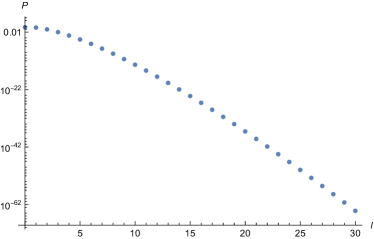
(a) $\beta=1,q=0.1$

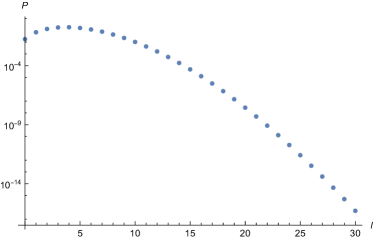
(b) $\beta=10,q=0.1$

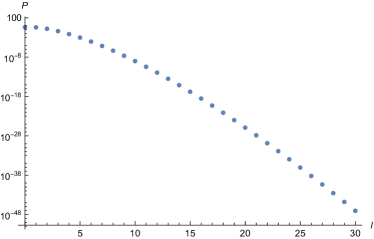
(c) $\beta=1,q=0.8$

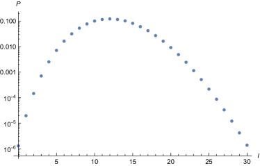
(d) $\beta=10,q=0.8$

Figure 1: Plot of $P_{\ell}(\beta,q)$ against $\ell$ for various values of $\beta$ and $q$.

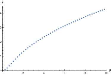
(a) $q=0.1$

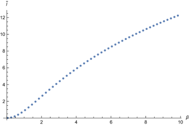
(b) $q=0.8$

Figure 2: Plot of $\overline{\ell}(\beta,q)$ against $\beta$ with fixed $q$.

6 Conclusions and outlook

In this paper, we have computed the HH wavefunction $\langle\ell|e^{-\beta T}|0\rangle$ in the DSSYK model explicitly, and we observed that the known result of un-crossed correlator of matter fields in Berkooz:2018jqr is obtained by gluing the HH wavefunctions with an appropriate weight. This observation suggests the bulk gravitational picture for the 2-point function in (52) and for the 4-point function in (59). Interestingly, the basic building block of the bulk spacetime is the chord and the spacetime can be thought of as fabric made of the chords (see e.g. (60)). This picture is vaguely reminiscent of the random tensor network Hayden:2016cfa or the bit threads Freedman:2016zud . As emphasized in Berkooz:2018qkz ; Berkooz:2018jqr ; Lin:2022rbf , in the DSSYK model the geodesic length is replaced by the number of chords $\ell$ which is naturally quantized. It would be very interesting to extract more information of the bulk spacetime from the DSSYK model.

There are many interesting open questions. The crossed 4-point function in DSSYK is constructed in Berkooz:2018jqr and it involves a complicated $R$-matrix originated from the underlying quantum group symmetry. It would be nice if we can extract the bulk spacetime picture of the crossed 4-point function. In particular we would like to understand the relation between the crossed 4-point function and the HH wavefunction as we did for the un-crossed case. It is also interesting to go beyond the strict large $N$ limit and compute the $1/N$ corrections. In the strict large $N$ limit (3), we only see the bulk spacetime with disk topology. It would be interesting to study the higher genus corrections to the DSSYK model and develop a technique to compute the higher genus corrections systematically. As a first step, it would be interesting to compute the DSSYK analogue of the “trumpet partition function”, which played an important role in the matrix model of JT gravity Saad:2019lba . We leave this as a very interesting future problem.

- (1) A. Kitaev, “A simple model of quantum holography (part 1),”. https://online.kitp.ucsb.edu/online/entangled15/kitaev/.
- (2) A. Kitaev, “A simple model of quantum holography (part 2),”. https://online.kitp.ucsb.edu/online/entangled15/kitaev2/.
- (3) S. Sachdev and J. Ye, “Gapless spin-fluid ground state in a random quantum heisenberg magnet,” Phys. Rev. Lett. 70 no. 21, (1993) 3339–3342, arXiv:cond-mat/9212030.
- (4) J. Maldacena and D. Stanford, “Remarks on the Sachdev-Ye-Kitaev model,” Phys. Rev. D 94 no. 10, (2016) 106002, arXiv:1604.07818 [hep-th].
- (5) J. Polchinski and V. Rosenhaus, “The Spectrum in the Sachdev-Ye-Kitaev Model,” JHEP 04 (2016) 001, arXiv:1601.06768 [hep-th].
- (6) R. Jackiw, “Lower Dimensional Gravity,” Nucl. Phys. B252 (1985) 343–356.
- (7) C. Teitelboim, “Gravitation and Hamiltonian Structure in Two Space-Time Dimensions,” Phys. Lett. 126B (1983) 41–45.
- (8) J. S. Cotler, G. Gur-Ari, M. Hanada, J. Polchinski, P. Saad, S. H. Shenker, D. Stanford, A. Streicher, and M. Tezuka, “Black Holes and Random Matrices,” JHEP 05 (2017) 118, arXiv:1611.04650 [hep-th]. [Erratum: JHEP 09, 002 (2018)].
- (9) M. Berkooz, P. Narayan, and J. Simon, “Chord diagrams, exact correlators in spin glasses and black hole bulk reconstruction,” JHEP 08 (2018) 192, arXiv:1806.04380 [hep-th].
- (10) M. Berkooz, M. Isachenkov, V. Narovlansky, and G. Torrents, “Towards a full solution of the large N double-scaled SYK model,” JHEP 03 (2019) 079, arXiv:1811.02584 [hep-th].
- (11) H. W. Lin, “The bulk Hilbert space of double scaled SYK,” JHEP 11 (2022) 060, arXiv:2208.07032 [hep-th].
- (12) J. B. Hartle and S. W. Hawking, “Wave Function of the Universe,” Phys. Rev. D 28 (1983) 2960–2975.
- (13) P. Saad, “Late Time Correlation Functions, Baby Universes, and ETH in JT Gravity,” arXiv:1910.10311 [hep-th].
- (14) P. Hayden, S. Nezami, X.-L. Qi, N. Thomas, M. Walter, and Z. Yang, “Holographic duality from random tensor networks,” JHEP 11 (2016) 009, arXiv:1601.01694 [hep-th].
- (15) M. Freedman and M. Headrick, “Bit threads and holographic entanglement,” Commun. Math. Phys. 352 no. 1, (2017) 407–438, arXiv:1604.00354 [hep-th].
- (16) P. Saad, S. H. Shenker, and D. Stanford, “JT gravity as a matrix integral,” arXiv:1903.11115 [hep-th].