Bound states around impurities in a superconducting bilayer

Abstract

We theoretically study the appearance of bound states around impurities in a superconducting bilayer. We focus our attention on $s$-wave pairing, which includes unconventional odd-parity states permitted by the layer degree of freedom. Utilizing numerical mean-field and analytical $T$-matrix methods, we survey the bound state spectrum produced by momentum-independent impurity potentials in this model. For even-parity $s$-wave pairing, bound states are only found for impurities which break time-reversal symmetry. For odd-parity $s$-wave states, in contrast, bound states are generically found for all impurity potentials, and fall into six distinct categories. This categorization remains valid for nodal gaps. Our results are conveniently understood in terms of the “superconducting fitness” concept, and show an interplay between the pair-breaking effects of the impurity and the normal-state band structure.

I Introduction

The robustness of conventional superconductors to the presence of non-magnetic impurities is famously guaranteed by Anderson’s theorem and the isotropic gap function Anderson (1959). However, if the disorder breaks time-reversal symmetry or the superconductor has an unconventional sign-changing gap, introducing a finite concentration of impurities rapidly suppresses the critical temperature to zero Mineev and Samokhin (1999). This pair-breaking effect is also evidenced by a single impurity with the appearance of bound states localized at the impurity with energy within the superconducting gap. So-called Yu-Shiba-Rusinov states were first proposed for magnetic impurities in conventional superconductors Yu (1965); Shiba (1968); Rusinov (1969). Impurity bound states also appear in fully-gapped unconventional superconductors for both magnetic and nonmagnetic impurities Wang and Wang (2004); Wang et al. (2012); Kim et al. (2015); Mashkoori et al. (2017), while subgap resonances appear in nodal superconductors due to the hybridization with the nodal quasiparticles Balatsky et al. (1995); Liu and Eremin (2008). Impurity bound states have attracted much attention over the last several decades Balatsky et al. (2006) as they can be directly detected by scanning tunneling microscopy experiments Yazdani et al. (1997), and hence act as a test of the pairing symmetry Hudson et al. (2001); Grothe et al. (2012). More recently, it has been claimed that topological superconductivity is realized in the bands formed by overlapping bound states on chains of magnetic impurities Nadj-Perge et al. (2014); Pawlak et al. (2016); Schneider et al. (2021).

Recently it has been observed that the superconductivity of Bi₂Se₃-based compounds is remarkably robust against disorder Kriener et al. (2012); Smylie et al. (2017); Andersen et al. (2020), despite strong evidence that it realizes a nematic odd-parity state which is not protected by Anderson’s theorem Yonezawa (2019). This has prompted interest in the possibility that the strong spin-orbit coupling (SOC) in this compound might be responsible for the enhanced robustness of the pairing state Michaeli and Fu (2012); Nagai et al. (2014); Nagai (2015); Andersen et al. (2020); Cavanagh and Brydon (2020, 2021); Dentelski et al. (2020); Sato and Asano (2020). Particular attention has been directed at the unconventional odd-parity $s$-wave states allowed by the sublattice structure of these materials Fu and Berg (2010), and it has been found that these states can be surprisingly robust against chemical potential disorder Michaeli and Fu (2012); Cavanagh and Brydon (2020, 2021). A key parameter in this theory is the “superconducting fitness” Ramires and Sigrist (2016); Ramires et al. (2018), which measures the degree to which the pairing state pairs electrons in the same band: the fitter the gap, the higher the degree of intraband pairing, and the weaker the suppression of the critical temperature by disorder. The fitness concept has also been extended to other impurity potentials, allowing the identification of impurities which are pair-breaking for a given pairing state Andersen et al. (2020); Timmons et al. (2020); Dentelski et al. (2020); Cavanagh and Brydon (2021).

Thus far the study of impurities in odd-parity $s$-wave superconductors has mainly focused upon the effect on the critical temperature Michaeli and Fu (2012); Andersen et al. (2020); Cavanagh and Brydon (2020, 2021); Dentelski et al. (2020); Sato and Asano (2020). The tuning of the pair-breaking effect by the normal-state band structure should nevertheless also influence the existence and structure of impurity bound states in such superconductors. This motivates us to study the bound states around an impurity in a minimal model with odd-parity $s$-wave states to clarify the role of superconducting fitness. Specifically, we consider impurities in a superconducting Rashba bilayer Nakosai et al. (2012) using two distinct methods: a numerical self-consistent mean-field theory for a tight-binding model, and an analytic non-self-consistent $T$-matrix theory. Examining all momentum-independent impurity potentials, we find that the bound states belong to distinct classes which depend on the symmetry of each impurity and its fitness with respect to a given pairing state. Bound states are still possible for fit impurities when the pairing state is unfit with respect to parts of the normal state Hamiltonian. Our results also hold for virtual bound states which appear when the pairing state has nodes.

Our paper is organized as follows: In Sec. II, we introduce the two-dimensional tight-binding bilayer model and our approximation schemes. We summarize the concept of superconducting fitness in Sec. II.1, while the self-consistent mean-field theory and the $T$-matrix approximation are introduced in Secs. II.2 and II.3, respectively. In Sec. III, we present our numerical and analytical results for the bound states and develop the classification scheme for the isotropic even-parity singlet state (Sec. III.1) and the fully-gapped odd-parity $s$-wave states (Sec. III.2). In Sec. IV we extend our analysis to nodal gaps in a three-dimensional continuum model, and find that our symmetry classification remains valid for the virtual bound states. In Sec. V we summarize our conclusions and discuss future work.

II Model and methods

As a minimal model we consider superconductivity in a two-dimensional square bilayer lattice with an impurity. This is described by the Hamiltonian

$$H=H_{0}+H_{\text{imp}}+H_{\text{int}}\,.$$ (1)

The first term describes the motion of the noninteracting electrons

$$H_{0}=\sum_{\mathbf{r_{i},r_{j}}}\mathbf{c}_{\mathbf{r_{i}}}^{\dagger}\mathcal{H_{\mathbf{r_{i},r_{j}}}}\mathbf{c_{\mathbf{r_{j}}}}\,,$$ (2)

where $\mathbf{c_{\mathbf{r_{j}}}}=(c_{A,\mathbf{r_{j}},\uparrow},c_{A,\mathbf{r_{j}},\downarrow},c_{B,\mathbf{r_{j}},\uparrow}c_{B,\mathbf{r_{j}},\downarrow})^{T}$, and $c_{\eta,\mathbf{r_{j}},\sigma}$ is the destruction operator for a spin-$\sigma$ electron on layer $\eta=A$, $B$ at $\mathbf{r_{j}}$, and the matrix elements are

$$\mathcal{H_{\mathbf{r_{i},r_{j}}}} = \left[-t(\delta_{\mathbf{r_{i},r_{j}}\pm a\hat{\bf x}}+\delta_{\mathbf{r_{i},r_{j}}\pm a\hat{\bf y}})-\mu\delta_{\mathbf{r_{i},r_{j}}}\right]\eta_{0}\sigma_{0}$$ (3)

$$+t_{\perp}\delta_{\mathbf{r_{i},r_{j}}}\eta_{x}\sigma_{0}+\lambda_{x,\mathbf{r_{i},r_{j}}}\eta_{z}\sigma_{x}+\lambda_{y,\mathbf{r_{i},r_{j}}}\eta_{z}\sigma_{y}\,,$$

where the $\sigma_{\mu}$ and $\eta_{\mu}$ are the Pauli matrices for spin and layer degrees of freedom, respectively, and $\eta_{\nu}\sigma_{\mu}$ is to be understood as a Kronecker product. The first line in Eq. 3 includes the intralayer nearest-neighbour hopping $t$ and the chemical potential $\mu$, the second line describes the coupling of the layers via the hopping $t_{\perp}$ between the $A$ and $B$ sites in each unit cell, and a Rashba SOC of strength $\alpha$ in each layer

$$\lambda_{x,\mathbf{r_{i},r_{j}}} = \pm\frac{\alpha}{2i}\delta_{\mathbf{r_{i},r_{j}}\pm a\hat{\bf y}}\,,$$ (4)

$$\lambda_{y,\mathbf{r_{i},r_{j}}} = \mp\frac{\alpha}{2i}\delta_{\mathbf{r_{i},r_{j}}\pm a\hat{\bf x}}\,.$$ (5)

The Rashba SOC is generically present as the $A$ and $B$ sites are not inversion centres Nakosai et al. (2012). To preserve the global inversion symmetry, which swaps the $A$ and $B$ layers, the Rashba SOC has an opposite sign in each layer as encoded by the $\eta_{z}$ Pauli matrix in Eq. 3.

The second term in Eq. 1 is

$$H_{\text{imp}}={\bf c}_{{\bf r_{0}}}^{\dagger}\hat{V}_{\text{imp}}{\bf c}_{{\bf r_{0}}}\,.$$ (6)

This describes an impurity located at site ${\bf r_{0}}$ which couples to the electrons via one of the sixteen impurity potentials tabulated in Table 2, i.e. $\hat{V}_{\text{imp}}=V^{\alpha\beta}\eta_{\alpha}\sigma_{\beta}$. We consider each impurity potential individually, i.e. we only take one of the $V^{\alpha\beta}=V$ to be nonzero at a time.

The layer degree of freedom allows for unconventional $s$-wave (i.e. intra-unit cell) paring states as listed in Table 1. We include these states in Eq. 1 via the phenomenological pairing interaction

$$H_{\text{int}}=\frac{g}{4}\sum_{\mathbf{r_{j}}}\left\{\left(\mathbf{c}^{\dagger}_{\mathbf{r_{j}}}\hat{\Delta}_{\nu}\mathbf{c}^{\dagger}_{\mathbf{r_{j}}}\right)\left(\mathbf{c_{r_{j}}}\hat{\Delta}_{\nu}\mathbf{c_{r_{j}}}\right)\right\},$$ (7)

where $g$ is the effective coupling constant and $\hat{\Delta}_{\nu}$ is one of $s$-wave pairing potentials. In the following we set the coupling constant to be nonzero in a single pairing channel at a time.

Performing a mean-field decoupling of the interaction Hamiltonian in the Cooper channel, we obtain the Bogoliubov-de Gennes (BdG) Hamiltonian

$$H_{\text{BdG}}=\frac{1}{2}\sum_{\mathbf{r_{i}},\mathbf{r_{j}}}\mathbf{\Psi}_{\mathbf{r_{i}}}^{\dagger}\begin{pmatrix}\mathcal{\tilde{H}_{\mathbf{r_{i},r_{j}}}}&\hat{\Delta}_{\mathbf{r_{i},r_{j}}}\\ \hat{\Delta}^{\dagger}_{\mathbf{r_{i},r_{j}}}&-\mathcal{\tilde{H}}^{T}_{\mathbf{r_{i},r_{j}}}\end{pmatrix}\mathbf{\Psi_{r_{j}}}\,.$$ (8)

Here $\mathbf{\Psi_{r_{j}}}=(\mathbf{c}^{T}_{\mathbf{r_{j}}},\mathbf{c}^{\dagger}_{\mathbf{r_{j}}})^{T}$ is an eight-component spinor of creation and annihilation operators, $\mathcal{\tilde{H}_{\mathbf{r_{i},r_{j}}}}=\mathcal{H_{\mathbf{r_{i},r_{j}}}}+\hat{V}_{\text{imp}}\delta_{\mathbf{r_{i},r_{0}}}\delta_{\mathbf{r_{j},r_{0}}}$, and the pairing term is given by

$$\hat{\Delta}_{\mathbf{r_{i},r_{j}}}=\frac{1}{2}\delta_{\mathbf{r_{i},r_{j}}}g\langle\mathbf{c_{r_{j}}}\hat{\Delta}_{\nu}\mathbf{c_{r_{j}}}\rangle\hat{\Delta}_{\nu},$$ (9)

where $\langle...\rangle$ represents the thermally-weighted expectation value.

II.1 Superconducting fitness

Due to the presence of the layer degree of freedom, the normal-state Hamiltonian Eq. 2 describes a two-band electronic system. Expressed in momentum space, the band energies are given by

$$E_{\pm,\mathbf{k}} = -2t\left(\cos(k_{x}a)+\cos(k_{y}a)\right)-\mu$$ (10)

$$\pm\sqrt{\alpha^{2}\text{sin}^{2}({k_{x}a})+\alpha^{2}\text{sin}^{2}({k_{y}a})+t_{\perp}^{2}}\,,$$

where $a$ is the lattice constant. The multiband nature has an important consequence for the superconductivity: Pairing can occur between electrons in both the same and different bands. Of the pairing potentials listed in Tab. 1, only the uniform singlet state pairs electrons in time-reversed states, which guarantees purely intraband pairing; the other superconducting states will in general involve both intra- and interband pairing.

The concept of the superconducting fitness has recently been developed as a way to quantify the degree of interband pairing Ramires and Sigrist (2016); Ramires et al. (2018). For the pairing potential $\hat{\Delta}=\Delta_{0}\hat{\Delta}_{\nu}$, where $\Delta_{0}$ is the amplitude and $\hat{\Delta}_{\nu}$ is a dimensionless matrix for pairing in channel $\nu$, we define the fitness function

$$F_{\nu,{\bm{k}}}={\cal H}_{0,{\bm{k}}}\hat{\Delta}_{\nu}-\hat{\Delta}_{\nu}{\cal H}^{T}_{0,-{\bm{k}}}\,,$$ (11)

which is only nonzero if the interband pairing is present. For the two-band system considered here the fitness can be related to the gap opened at the Fermi energy

$$\Delta_{\text{eff},{\bm{k}}}=|\Delta_{0}|\sqrt{1-\tilde{F}_{\nu,\bm{k}}}\,,$$ (12)

where

$$\tilde{F}_{\nu,\bm{k}}=\frac{\text{Tr}\{|F_{\nu,{\bm{k}}}|^{2}\}}{(E_{+,{\bm{k}}}-E_{-,{\bm{k}}})^{2}}\,.$$ (13)

Eq. 13 takes values between $0$ and $1$, with $\tilde{F}_{\nu,{\bm{k}}}=0$ indicating a perfectly “fit” pairing state where there is only intraband pairing and thus the gap is maximal, whereas $\tilde{F}_{\nu,{\bm{k}}}=1$ implies that only interband pairing is present and no gap is opened at the Fermi energy at weak coupling.

The concept of superconducting fitness has been extended to the impurity potential Cavanagh and Brydon (2021). In a two-band system, whether or not the impurity is pair-breaking in the channel $\nu$ is given by the solution of

$$\hat{V}_{\text{imp}}\hat{\Delta}_{\nu}-\lambda\hat{\Delta}_{\nu}\hat{V}_{\text{imp}}^{T}=0\,,$$ (14)

where $\lambda=-1$ ($1$) implies that the impurity is (is not) pair-breaking. In the case of on-site singlet pairing this is equivalent to whether or not the impurity breaks time-reversal symmetry, and is thus a restatement of Anderson’s theorem Anderson (1959); for the nontrivial $s$-wave pairing potentials Eq. 14 therefore establishes a generalized Anderson’s theorem. An important difference compared to the usual Anderson’s theorem is that the critical temperature of the odd-parity $s$-wave states is generally suppressed even when the impurity is not pair-breaking if the fitness $0<\tilde{F}_{\nu,\bm{k}}<1$, albeit more slowly compared to the usual Gor’kov theory Mineev and Samokhin (1999).

II.2 Real-space mean-field theory

We solve the self-consistency equations Eq. 9 for the pairing potential in real-space by diagonalizing the BdG Hamiltonian Eq. 8 implemented on a finite lattice with periodic boundary conditions Zhu (2016). For the calculations of the impurity bound state spectrum we choose a $31\times 31$ lattice with the impurity located at the center.

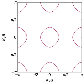
Figure 1: The Fermi surface of the bilayer model with $k_{\text{F}}a=0.9$.

The four parameters $(t,\mu,t_{\perp},\alpha)$ of our tight-binding model describe a large variety of different band structures. Although our primary aim is to understand the influence of the intertwined spin and layer degrees of freedom on the impurity bound state spectrum, the bound states can also be influenced by the shape of the Fermi surface and the Fermi velocity Ortuzar et al. (2022); Uldemolins et al. (2022). To control for this variation we observe that in the absence of intralayer hopping $t=0$, the iso-energy lines of the bands Eq. 10 in the Brillouin zone are the same for all parameter choices so long as $\alpha\neq 0$. Thus, for fixed filling, the shape of the Fermi surface is the same for all values of $t_{\perp}$ and $\alpha$. This is equivalent to setting the chemical potential to be

$$\mu=\alpha\sqrt{\text{sin}^{2}({k_{\text{F}}a})+\left(\frac{t_{\perp}}{\alpha}\right)^{2}},$$ (15)

for some fixed $k_{\text{F}}$; in the following we choose $k_{\text{F}}a=0.9$ which gives the Fermi surface shown in Fig. 1. Since the intralayer hopping appears with the identity matrix in Eq. 3, it does not influence the gap at the Fermi surface, and we thus do not expect that setting $t=0$ will qualitatively affect our results. This assumption will later be verified using the analytic $T$-matrix theory in Sec. II.3.

The Fermi velocity in our model is given by

$${\mathbf{v}_{k}}=\frac{\alpha^{2}a}{2\mu}\left(\sin(2k_{x}a)\hat{\bf x}+\sin(2k_{y}a)\hat{\bf y}\right)\,,$$ (16)

where $k_{x}$ and $k_{y}$ lie on the Fermi surface $\sin^{2}(k_{x}a)+\sin^{2}(k_{y}a)=\sin^{2}(k_{\text{F}}a)$. The magnitude of the Fermi velocity decreases with increasing $t_{\perp}$, which should reduce the coherence length even for fixed pairing potential, and may affect the impurity bound state spectrum. We keep the Fermi velocity constant by scaling $\alpha$ as

$$\alpha=\frac{\alpha_{0}}{\sqrt{2}}\left(1+\sqrt{1+\frac{4t_{\perp}^{2}}{\alpha_{0}^{2}\text{sin}^{2}({k_{\text{F}}a})}}\right)^{1/2},$$ (17)

where $\alpha_{0}$ is the value of $\alpha$ at $t_{\perp}=0$. In the following we set $\alpha_{0}$ as the unit of energy. For fixed $k_{\text{F}}a$, the normal-state properties of the bilayer model now only depend on the ratio $t_{\perp}/\alpha_{0}$.

description	matrix	irrep	effective gap (2D)	effective gap (3D)
uniform intralayer singlet	$\Delta_{0}\eta_{0}i\sigma_{y}$	$A_{\text{1g}}$	$\Delta_{0}$	$\Delta_{0}$
interlayer singlet	$\Delta_{0}\eta_{x}i\sigma_{y}$	$A_{\text{1g}}$	$\Delta_{0}|\tilde{t}_{\perp}|$	$\Delta_{0}|\tilde{m}|$
staggered intralayer singlet	$\Delta_{0}\eta_{z}i\sigma_{y}$	$A_{\text{2u}}$	$\Delta_{0}\sqrt{1-\tilde{t}_{\perp}^{2}}$	$\Delta_{0}\tilde{v}\sqrt{k_{x}^{2}+k_{y}^{2}}$
interlayer triplet	$\Delta_{0}\eta_{y}\sigma_{z}i\sigma_{y}$	$A_{\text{1u}}$	$\Delta_{0}\sqrt{1-\tilde{t}_{\perp}^{2}}$	$\Delta_{0}\sqrt{1-\tilde{m}^{2}}$
interlayer triplet	$\{\Delta_{0}\eta_{y}\sigma_{x}i\sigma_{y},$ $\Delta_{0}\eta_{y}\sigma_{y}i\sigma_{y}\}$	$E_{\text{u}}$	$\{\Delta_{0}\tilde{\alpha}|\sin(k_{y}a)|,\Delta_{0}\tilde{\alpha}|\sin(k_{x}a)|\}$	$\{\Delta_{0}\tilde{v}\sqrt{k_{y}^{2}+k_{z}^{2}},\Delta_{0}\tilde{v}\sqrt{k_{x}^{2}+k_{z}^{2}}\}$

Table 1: Summary of possible $s$-wave pairing states in a bilayer superconductor. The columns give the description, the matrix form, the irreducible representation, and the value of the effective gap at the Fermi surface of the two models considered here. We adopt the short-hand notation $\tilde{t}_{\perp}=t_{\perp}/\mu$ and $\tilde{\alpha}=\alpha/\mu$.

The effective gap of the six $s$-wave pairing states at the Fermi energy is given in Table. 1. All but the uniform singlet depend on the parameters of the model, reflecting the pair-breaking by the spin-layer texture of the normal-state band wavefunctions. Importantly, we see that the $A_{\text{1g}}$, $A_{\text{1u}}$, and $A_{\text{2u}}$ produce full isotropic gaps at the Fermi energy. In contrast, the two $E_{\text{u}}$ states have point nodes. Since impurity bound states are only well-defined in the presence of a full gap, we will not examine the $E_{\text{u}}$ states within the mean-field theory; the impurity virtual bound states which appear in these cases will be analyzed using the $T$-matrix theory developed below. Moreover, we will also not present results for the nontrivial $A_{\text{1g}}$ state, as this is essentially equivalent to the trivial $A_{\text{1g}}$ state when only a single band crosses the Fermi energy Cavanagh and Brydon (2021). In solving the mean-field equations, the effective coupling constant $g$ in Eq. 7 is chosen such that the pairing amplitude $\Delta_{0}=\frac{g}{2}\langle\mathbf{c_{r_{j}}}\hat{\Delta}_{\nu}\mathbf{c_{r_{j}}}\rangle=0.08\alpha_{0}$ in the absence of the impurity.

II.3 $T$-matrix theory

To complement the numerical mean-field calculation we also study the appearance of bound states at the impurity site within the $T$-matrix approximation. This has the benefit that it can be performed analytically if we relax the self-consistency requirement Eq. 9, i.e. we treat $\Delta_{0}=\frac{g}{2}\langle\mathbf{c_{r_{j}}}\hat{\Delta}_{\nu}\mathbf{c_{r_{j}}}\rangle$ as independent of $\mathbf{r_{j}}$.

The non-self-consistent $T$ matrix is defined as

$$T(i\omega_{n})=\left[\hat{\mathbf{1}}-\hat{V}_{\text{imp}}G_{0}(i\omega_{n})\right]^{-1}\hat{V}_{\text{imp}}\,,$$ (18)

where $\hat{V}_{\text{imp}}$ is the impurity potential in Nambu grading and

$$G_{0}(i\omega_{n})=\frac{1}{N}\sum_{\bf k}G_{0}({\bf k},i\omega_{n})\,,$$

is the momentum-average of the Green’s function $G_{0}({\bf k},i\omega_{n})$ of the superconductor in the absence of the impurity, with $N$ the number of lattice points.

Analytic expressions for the Green’s functions are complicated and the exact evaluation of the momentum sum in Eq. 18 is difficult. To make progress, we replace the sum with an integral over energy near the Fermi surface and a Fermi-surface average

$$\frac{1}{N}\sum_{\bf k}\to\int_{-\Lambda}^{\Lambda}N\left(\xi\right)d\xi\langle\ldots\rangle_{\text{FS}}.$$ (19)

where ${N}(\xi)$ is the density of states (DOS) and $\Lambda$ is an energy cutoff. Although analytic expressions for the DOS of the tight-binding model exist, here we pursue a more general approach by adopting a linear approximation to the DOS

$${N}\left(\xi\right)={N}_{0}+\xi{N}_{0}^{\prime}.$$ (20)

where ${N}_{0}$ is the DOS at the Fermi energy and ${N}_{0}^{\prime}$ is the first-order derivative with respect to energy. The parameter ${N}_{0}^{\prime}$ reflects the particle-hole asymmetry of the DOS. Although the presence of particle-hole asymmetry is not essential for the formation of bound states, it is necessary for achieving quantitative agreement with the tight-binding model.

Using these approximations, the momentum-averaged Green’s functions for the three pairing states are

$$G_{0}(i\omega_{n})=-i\omega_{n}g_{0}(\eta_{0}+\tilde{t}_{\perp}\eta_{x})\sigma_{0}\tau_{0}-y(\eta_{0}+\tilde{t}_{\perp}\eta_{x})\sigma_{0}\tau_{z}-\begin{cases}g_{0}\Delta_{\text{eff}}^{A_{\text{1g}}}(\eta_{0}-\tilde{t}_{\perp}\eta_{x})i\sigma_{y}\tau_{x}&A_{\text{1g}}\\ g_{0}\Delta_{\text{eff}}^{A_{\text{1u}}}\sqrt{1-\tilde{t}_{\perp}^{2}}\eta_{y}\sigma_{x}\tau_{x}&A_{\text{1u}}\\ g_{0}\Delta_{\text{eff}}^{A_{\text{2u}}}\sqrt{1-\tilde{t}_{\perp}^{2}}\eta_{z}\sigma_{y}\tau_{y}&A_{\text{2u}}\end{cases}\,,$$ (21)

where $\tau_{j}$ are the Pauli matrices in Nambu space and its product with $\eta$ and $\sigma$ matrices implies a Kronecker product, $\tilde{t}_{\perp}=t_{\perp}/\mu$, and

$$g_{0}=\frac{{N}_{0}\pi}{2\sqrt{\omega_{n}^{2}+\Delta_{\text{eff}}^{2}}}\,.$$ (22)

The parameter $y\approx{N}^{\prime}_{0}\Lambda$ encodes the particle-hole asymmetry, and we treat it as a fitting parameter. A sketch of the derivation of Eq. 21 is provided in appendix A. In particular, we show that Eq. 21 is valid for any band structure where only a single band crosses the Fermi energy. This gives us confidence that our results hold beyond the restricted parameter space chosen for the lattice model where we set $t=0$.

The relatively simple form of the integrated Green’s function allows us to evaluate the $T$ matrix Eq. 18 analytically. The impurity bound states are then determined by making the analytic continuation $i\omega_{n}\rightarrow\omega+i0^{+}$ and solving for the poles at subgap energies $|\omega|<\Delta_{\text{eff}}$. In the following, we express our results in turns of dimensionless quantities $\tilde{\omega}=\omega/|\Delta_{\text{eff}}|$, $\tilde{V}=\frac{\pi}{2}N_{0}V$ and $\tilde{y}=y/(\frac{\pi}{2}N_{0})$.

		impurity
		$\eta_{0}\sigma_{0}$	$\eta_{x}\sigma_{0}$	$\eta_{y}\sigma_{0}$	$\eta_{z}\sigma_{x}$	$\eta_{z}\sigma_{y}$	$\eta_{z}\sigma_{z}$	$\eta_{z}\sigma_{0}$	$\eta_{y}\sigma_{x}$	$\eta_{y}\sigma_{y}$	$\eta_{y}\sigma_{z}$	$\eta_{x}\sigma_{x}$	$\eta_{x}\sigma_{y}$	$\eta_{x}\sigma_{z}$	$\eta_{0}\sigma_{x}$	$\eta_{0}\sigma_{y}$	$\eta_{0}\sigma_{z}$
symmetry	$\mathcal{T}$	✓	✓	✗	✗	✗	✗	✓	✓	✓	✓	✗	✗	✗	✗	✗	✗
	$\mathcal{PT}$	✓	✓	✓	✓	✓	✓	✗	✗	✗	✗	✗	✗	✗	✗	✗	✗
fitness	$A_{\text{1g}}$	$+1$	$+1$	$-1$	$-1$	$-1$	$-1$	$+1$	$+1$	$+1$	$+1$	$-1$	$-1$	$-1$	$-1$	$-1$	$-1$
	$A_{\text{1u}}$	$+1$	$-1$	$-1$	$-1$	$-1$	$+1$	$-1$	$-1$	$-1$	$+1$	$-1$	$-1$	$+1$	$+1$	$+1$	$-1$
	$A_{\text{2u}}$	$+1$	$-1$	$+1$	$-1$	$-1$	$-1$	$+1$	$-1$	$-1$	$-1$	$+1$	$+1$	$+1$	$-1$	$-1$	$-1$
	$E_{\text{u},x}$	$+1$	$-1$	$-1$	$-1$	$+1$	$-1$	$-1$	$-1$	$+1$	$-1$	$-1$	$+1$	$-1$	$+1$	$-1$	$+1$
	$E_{\text{u},y}$	$+1$	$-1$	$-1$	$+1$	$-1$	$-1$	$-1$	$+1$	$-1$	$-1$	$+1$	$-1$	$-1$	$-1$	$+1$	$+1$
classification	$A_{\text{1g}}$	-	-	a*	a*	a*	a*	-	-	-	-	b*	b*	b*	b*	b*	b*
	$A_{\text{1u}}$	a	b	d	d	d	c	d	d	d	c	f	f	e	e	e	f
	$A_{\text{2u}}$	a	b	c	d	d	d	c	d	d	d	e	e	e	f	f	f
	$E_{\text{u},x}$	a	b	d	d	c	d	d	d	c	d	f	e	f	e	f	e
	$E_{\text{u},y}$	a	b	d	c	d	d	d	c	d	d	e	f	f	f	e	e

Table 2: Categorization of bound state spectra for the $s$-wave states considered in this paper. The symmetry row shows whether the impurity preserves/breaks (✓/ ✗) time-reversal symmetry $\mathcal{T}$ and combined parity-time-reversal symmetry $\mathcal{PT}$. The fitness row indicates the solution for $\lambda$ in Eq. 14, with $\lambda=+1$ ($-1$) indicating a fit (unfit) impurity for each pairing state. The final row shows the classification of the bound states. For the $A_{\text{1g}}$ pairing, bound states only appear for time-reversal symmetry-breaking impurities, and we find two categories a^∗ and b^∗, respectively corresponding to the panels (a) and (b) in Fig.s 2 and 3. For the odd-parity $A_{\text{1u}}$ and $A_{\text{2u}}$ states we find six different categories a-f, corresponding to the panels (a)-(f) in Fig.s 4 and 5. For the $A_{\text{2u}}$ and $E_{\text{u}}$ pairing states, this classification also holds for the virtual bound states in Fig. 7.

III Bound states

The central result of our work is that the bound states which form around impurities fall into a number of distinct classes, which exhibit qualitatively different behavior as a function of interlayer coupling $\tilde{t}_{\perp}$ and impurity strength $\tilde{V}$. The classification of the 16 possible momentum-independent impurities for the different pairing states is summarized in Table 2, and is based on whether the impurity preserves time-reversal ($\mathcal{T}$) or combined parity-time-reversal ($\mathcal{PT}$) symmetries, and the fitness of the impurity with respect to the pairing state. $A_{\text{1g}}$ interlayer pairing this gives rise to three distinct categories of the spectrum, whereas for the $A_{\text{1u}}$ and $A_{\text{2u}}$ states there are six categories.

Before discussing the distinct cases in detail, we first comment on the significance of time-reversal ($\mathcal{T}$) or combined parity-time-reversal ($\mathcal{PT}$) symmetry. As these are both antiunitary symmetries, Kramers’ theorem dictates that the spectrum is two-fold degenerate when either is present. Since the clean BdG Hamiltonian is symmetric under both time-reversal and inversion, their presence or absence is determined entirely by the impurity.

III.1 $A_{\text{1g}}$ intralayer singlet pairing

The intralayer singlet $A_{\text{1g}}$ state pairs electrons in time-reversed states, and is thus subject to Anderson’s theorem. Since the normal state Hamiltonian has time-reversal symmetry, this state is perfectly fit in the clean limit and there is only intraband pairing. The only pair-breaking impurities are those that break time-reversal symmetry, and we accordingly only find bound states around the impurities in these cases, as shown as a function of impurity strength and interlayer coupling in Fig. 2 and 3, respectively. These figures also show the excellent quantitative agreement between the mean-field and the $T$-matrix theories. Analytic expressions for the bound states obtained via the $T$-matrix method are complicated and are given in the appendix B.1.

Our results reveal two distinct classes of bound states: class (a) impurities where the bound states are two-fold degenerate, and class (b) impurities where the bound states are not degenerate. The degeneracy of the states in case (a) is ensured by a generalized Kramers’ theorem based on the preserved $\mathcal{PT}$ symmetry; in contrast, in case (b) both $\mathcal{T}$ and $\mathcal{PT}$ symmetries are broken, and there is no symmetry enforcing degeneracy. We note that even in case (b) the spectra is two-fold degenerate in the case of vanishing interlayer coupling.

\begin{overpic}[width=223.31403pt,keepaspectratio]{fitYG.pdf} \put(3.0,2.0){(a)} \put(50.0,2.0){(b)} \end{overpic}

Figure 2: Subgap spectrum as a function of the dimensionless impurity strength $\tilde{V}$ for the intralayer singlet $A_{\text{1g}}$ pairing. Plots (a) and (b) correspond to the impurity classifications for this pairing state tabulated in Table 2. The circles are the results of the self-consistent mean-field theory. The dashed grey line is the analytic prediction for the gap edge, and the solid red line represents the results of the analytic $T$-matrix theory for the subgap states. The interlayer impurity hopping is set as $\tilde{t}_{\perp}=0.54$ and the particle-hole asymmetric strength is set as $\tilde{y}=0.50$.

\begin{overpic}[width=223.31403pt,keepaspectratio]{fitYGTNew.pdf} \put(3.0,2.0){(a)} \put(50.0,2.0){(b)} \end{overpic}

Figure 3: Subgap spectrum as a function of the dimensionless interlayer hopping $\tilde{t}_{\perp}$ for the intralayer singlet $A_{\text{1g}}$ pairing. Plots (a)-(d) correspond to the four possible impurity classifications for this pairing state tabulated in Table 2. The normalized impurity strength is set as $\tilde{V}=0.64$ and the particle-hole asymmetric strength is set as $\tilde{y}=0.50$. The same style is used as in Fig. 2.

III.2 Odd-parity $A_{\text{1u}}$ and $A_{\text{2u}}$ states

We now turn to the bound state spectrum in the case of the fully-gapped odd-parity states, which is considerably richer than the $A_{\text{1g}}$ state. The classification of the spectra is the same for the two odd-parity states, reflecting the fact that in the clean limit the BdG Hamiltonian is the same up to unitary transformation, specifically we have

$${\cal H}_{\text{BdG},A_{\text{2u}}}=U^{\dagger}{\cal H}_{\text{BdG},A_{\text{1u}}}U\,,$$ (23)

where ${\cal H}_{\text{BdG},A_{\text{1u}}(A_{\text{2u}})}$ is the BdG Hamiltonian matrix for the $A_{\text{1u}}$ ($A_{\text{2u}}$) state in the absence of the impurity, and

$$U=\begin{pmatrix}\exp(i\frac{\pi}{4}\eta_{x}\sigma_{z})&0\\ 0&\exp(-i\frac{\pi}{4}\eta_{x}\sigma_{z})\end{pmatrix}.$$ (24)

The impurity potential is generally not invariant under this unitary transform: this allows us to map each impurity potential in the $A_{\text{1u}}$ pairing state to another impurity potential in the $A_{\text{2u}}$ pairing state. It also follows from Eq. 23 that the fitness of the $A_{\text{1u}}$ and $A_{\text{2u}}$ states are the same in the clean limit, with both pairing states unfit with respect to the interlayer coupling $t_{\perp}$. Both states are perfectly fit when $t_{\perp}=0$, and in this limit there also exists a unitary transformation that maps the odd-parity state to the $A_{\text{1g}}$ intralayer singlet state Fu and Berg (2010). We therefore expect that the bound states for the odd-parity $s$-wave pairing will strongly depend on the interlayer coupling.

We find six different classes of bound state spectra, which are shown in Figs. 4 and 5 as a function of $\tilde{V}$ and $\tilde{t}_{\perp}$, respectively. There is again excellent agreement between the self-consistent real-space lattice theory and the continuum $T$-matrix approximation, using the same particle-hole asymmetry parameter $\tilde{y}=0.50$ as for the $A_{\text{1g}}$ results. The dependence on the impurity strength shows a clear difference between the fit impurities (cases (a), (c), and (e)) and the unfit impurities (cases (b), (d), and (f)): although bound states are generally present, only for the unfit impurities do the bound states cross zero energy as a function of impurity strength. The closing of the gap by the impurity evidence the pair-breaking nature of the unfit impurities. The role of the fitness with respect to the normal-state Hamiltonian is clearly revealed by the dependence on the interlayer coupling $t_{\perp}$ shown in Fig. 5: bound states for the fit impurities are always absent for vanishing intralayer coupling, as anticipated by the mapping between the odd-parity and the $A_{\text{1g}}$ states.

\begin{overpic}[width=223.31403pt,keepaspectratio]{fitY.pdf} \put(3.0,67.0){(a)} \put(50.0,67.0){(b)} \put(3.0,34.5){(c)} \put(50.0,34.5){(d)} \put(3.0,2.0){(e)} \put(50.0,2.0){(f)} \end{overpic}

Figure 4: Subgap spectrum as a function of the dimensionless impurity strength $\tilde{V}$ for the odd-parity $A_{\text{1u}}$ or $A_{\text{2u}}$ pairing states. Plots (a)-(f) correspond to the six possible impurity classes summarized in Table 2. The interlayer impurity hopping is set as $\tilde{t}_{\perp}=0.54$ and the particle-hole asymmetric strength is set as $\tilde{y}=0.50$. The same style is used as in Fig. 2.

\begin{overpic}[width=223.31403pt,keepaspectratio]{fitYt.pdf} \put(3.0,67.0){(a)} \put(50.0,67.0){(b)} \put(3.0,34.5){(c)} \put(50.0,34.5){(d)} \put(3.0,2.0){(e)} \put(50.0,2.0){(f)} \end{overpic}

Figure 5: Subgap spectrum as a function of the dimensionless interlayer hopping $\tilde{t}_{\perp}$ for the odd-parity $A_{\text{1u}}$ or $A_{\text{2u}}$ pairing states. Plots (a)-(f) correspond to the six possible impurity classes summarized in Table 2. The normalized impurity strength is set as $\tilde{V}=0.64$ and the particle-hole asymmetric strength is set as $\tilde{y}=0.50$. The same style is used as in Fig. 2.

Greater insight is provided by the analytic expressions for the bound states found in the $T$-matrix theory. These expressions are generally rather complicated, so to more clearly reveal the relationship we set $\tilde{y}=0$; general expressions with $\tilde{y}\neq 0$ are provided in Appendix B.2. In the particle-hole-symmetric limit, the bound states are

$$\tilde{\omega}=\pm\frac{\lambda+\left(1-\tilde{t}_{\perp}^{2}\right)\tilde{V}^{2}}{\sqrt{1+2(1+S_{t_{\perp}}\tilde{t}_{\perp}^{2})\tilde{V}^{2}+(1-\tilde{t}_{\perp}^{2})^{2}\tilde{V}^{4}}}\,,$$ (25)

where $\lambda=\pm 1$ is the solution to Eq. 14 (i.e. the fitness of the impurity), and the parameter $S_{t_{\perp}}=+1$ ($-1$) according as the impurity commutes (anticommutes) with the interlayer hopping term. The combinations of $(S_{t_{\perp}},\lambda)$ give rise to four distinct bound state spectra: $(1,1)$ corresponding to cases (a) and (e), $(1,-1)$ corresponding to (b) and (f), $(-1,1)$ corresponding to (c), and $(-1,-1)$ corresponding to (d). The difference between the (a) and (e) (or (b) and (f)) cases is only apparent for nonzero asymmetry parameter $\tilde{y}$. In particular, a nonzero value of the asymmetry parameter is necessary to lift the two-fold degeneracy of the bound states, and is also responsible for the asymmetric dependence on the impurity potential seen in cases (a) and (b), and the interlayer coupling strength in case (b). These effects of the asymmetry parameter are consistent with previous work Wang et al. (2012); Mashkoori et al. (2017).

Despite these limitations, Eq. 25 nevertheless reveals the role of fitness. We first consider the different impurity fitness cases, $\lambda=\pm 1$: in the case of the fit impurity $\lambda=1$, the numerator of Eq. 25 is always positive and so the impurity cannot close the gap; on the other hand, for unfit impurities $\lambda=-1$ the numerator vanishes at a critical value $\tilde{V}=1/\sqrt{1-\tilde{t}_{\perp}^{2}}$, thus closing the gap. We also observe that the bound-state energies depend nontrivially on the interlayer coupling, reflecting the interplay of the impurity with the spin and layer degrees of freedom of the clean Hamiltonian, and thus the normal-state fitness of the pairing potential. The dependence on $S_{t_{\perp}}$ is generally more subtle, but in the case $S_{t_{\perp}}=-1$ it ensures that the term under the square root is a complete square. For $\lambda=1$ this cancels the numerator, and thus there are no subgap states due to the impurity.

The parameters $S_{t_{\perp}}$ and $\lambda$ also enter the Born approximation result for the suppression of the critical temperature by the presence of a finite concentration $n_{\text{imp}}$ of impurities Cavanagh and Brydon (2020, 2021). Here the critical temperature is given by the solution of the equation

$$\log\left(\frac{T_{c}}{T_{c0}}\right)=\Psi\left(\frac{1}{2}\right)-\Psi\left(\frac{1}{2}+\frac{1}{4\pi k_{B}T_{c}\tau}\right)\,,$$ (26)

where $T_{c0}$ is the critical temperature in the clean limit and the effective scattering rate is

$$\tau^{-1}=\pi n_{\text{imp}}|V|^{2}{N}_{0}\left(1+S_{t_{\perp}}\tilde{t}_{\perp}^{2}-\lambda\langle 1-\tilde{F}_{\nu,{\bm{k}}}\rangle_{\text{FS}}\right)\,.$$ (27)

The first two terms inside the brackets give the normal-state scattering rate, while the bulk fitness parameter Eq. 13 controls the effective scattering rate in the superconducting state. For the unfit impurities with $\lambda=-1$ the effective scattering rate is higher than the normal-state scattering rate, and the critical temperature is thus suppressed by increasing impurity concentration faster than the Abrikosov-Gor’kov predictions for an odd-parity state Mineev and Samokhin (1999); Conversely, the fit impurities with $\lambda=1$ have a lower effective scattering rate than in the normal-state, and so the critical temperature displays a weaker suppression than predicted by the usual theory. Intriguingly, in case (c) with $(S_{t_{\perp}},\lambda)=(-1,1)$, the scattering rate vanishes, implying that there is no suppression of the critical temperature. Our results are consistent with the observation that the presence of impurity bound states, even when produced by the fit impurities, indicates some degree of pair-breaking.

III.3 Sublattice localized impurities

A general impurity potential may involve a linear combination of all the matrices listed in Tab. 2, and hence includes both fit and unfit components. Since the formation of bound states is a nonlinear effect we cannot directly infer the bound state spectrum of a general impurity potential from the spectra produced by each component. A physically-interesting case of a multi-component impurity has the impurity potential localized on a single sublattice, i.e. arising from the replacement of an atom at a particular sublattice site by another species. The corresponding impurity potential has the matrix form $(\eta_{0}\pm\eta_{z})\sigma_{\mu}$, which involves two matrices which generally belong to different classes in Tab. 2.

In Fig. 6 we plot the subgap spectrum for sublattice-localized potential ($\mu=0$) and magnetic ($\mu=x$, $y$, $z$) impurities in the two odd-parity states. For both pairing states the subgap spectrum is independent of the polarization of the magnetic impurity. For the $A_{2u}$ state, the two components of the potential (magnetic) impurity are both fit (unfit). Consistent with our argument above, only the the subgap states of the unfit magnetic impurity cross zero energy.

The situation with the $A_{1u}$ state is more subtle, as for both potential and magnetic impurities one component is fit and the other is unfit. In the particle-hole-symmetric limit (i.e. $\tilde{y}=0$), the subgap states asymptotically go to zero at infinite impurity strength; switching on particle-hole asymmetry shifts the zero-crossing to a finite value of $\tilde{V}$. Thus, the presence of the unfit impurity potential is still consistent with the appearance of a zero-crossing of the subgap states.

\begin{overpic}[width=223.31403pt,keepaspectratio]{ComfitV.pdf} \put(3.0,34.5){(a)} \put(50.0,34.5){(b)} \put(3.0,2.0){(c)} \put(50.0,2.0){(d)} \end{overpic}

Figure 6: Subgap spectrum for sublattice-localized impurities as a function of the dimensionless impurity strength $\tilde{V}$ for odd-parity $A_{\text{1u}}$ (left) or $A_{\text{2u}}$ (right) pairing states. The top (bottom) row corresponds to potential (magnetic) impurities localized to a single sublattice. The interlayer impurity hopping is set as $\tilde{t}_{\perp}=0.54$ and the particle-hole asymmetric strength is set as $\tilde{y}=0.50$. The same style is used as in Fig. 2.

IV Three-dimensional model

The full gap of the $A_{\text{1u}}$ and $A_{\text{2u}}$ states in the two-dimensional tight-binding model is convenient for numerical calculations. However, in three dimensions the $A_{\text{2u}}$ state generically has point nodes. Due to hybridization with the low-lying quasiparticle states in the vicinity of these nodes, the impurity bound states found above are replaced by resonances or so-called virtual bound states Zhu (2016); Balatsky et al. (1995, 2006). Although it is numerically prohibitive to study the subgap spectra of the three-dimensional system using the tight-binding mean-field theory, the non-self-consistent $T$-matrix approximation can be readily applied to this problem. Considering the excellent agreement between the mean-field theory and the $T$-matrix approximation observed above for the two-dimensional model, we expect that the $T$-matrix approximation will also give accurate results in three dimensions.

IV.1 Minimal model

Close to the $\Gamma$ point, and keeping terms up to linear order in momentum, a minimal three-dimensional generalization of our normal-state Hamiltonian is

$$H({\bm{k}})= -\mu\eta_{0}\sigma_{0}+m\eta_{x}\sigma_{0}+v_{z}k_{z}\eta_{y}\sigma_{0}$$

$$+vk_{x}\eta_{z}\sigma_{y}-vk_{y}\eta_{z}\sigma_{x}\,,$$ (28)

where $m$ is the mass term, $v$ is the in-plane velocity, and $v_{z}$ is the out-of-plane velocity. The presence of the out-of-plane velocity $v_{z}$ extends the model to three dimensions; scaling the $z$-component of the momentum allows us to eliminate the velocity anisotropy, i.e. in the following we set $v_{z}=v$. In terms of the parameters of the tight-binding model we have $m=t_{\perp}$ and $v=\alpha a$. We note that a term proportional to $\eta_{z}\sigma_{z}$ is allowed by symmetry, but we neglect it as it appears with much higher power of momenta: for the tetragonal system considered here it requires taking the momentum expansion to the fifth order, whereas for trigonal or hexagonal systems it appears at the third order.

IV.2 $A_{\text{1g}}$ and $A_{\text{1u}}$ pairing states

The momentum-averaged Green’s function for both the $A_{\text{1g}}$ and $A_{\text{1u}}$ pairing states in the three-dimensional model is the same as in Eq. 21, and thus the conclusions of Sec. III remain valid. We note that including the $\eta_{z}\sigma_{z}$ term in the Hamiltonian does introduce some gap anisotropy for the $A_{\text{1u}}$ state and may therefore modify our results. So long as this term is small compared to the other terms in Eq. 28, however, we expect that the effects on the bound state spectrum will be small.

IV.3 $A_{\text{2u}}$ pairing state

The gap opened by the $A_{\text{2u}}$ pairing state on a three-dimensional Fermi surface is required by symmetry to have a node along the $k_{z}$ axis Mineev and Samokhin (1999). In our model, the gap at the Fermi energy is given by

$$\Delta_{A_{\text{2u}}}({\bm{k}})= \Delta_{0}\tilde{v}\sqrt{k_{x}^{2}+k_{y}^{2}},$$ (29)

where $\tilde{v}=v/\mu$. Restricted to the $k_{z}=0$ plane we recover the two-dimensional theory, with a uniform gap $\Delta_{0}\sqrt{1-\tilde{m}^{2}}$.

The derivation of the momentum-averaged Green’s function $G_{0}(\omega)$ is quite similar to that in Appendix A, except that accounting for the variation of the gap over the Fermi surface gives a more complicated frequency-dependence:

$$G_{0}(\omega)= -\frac{N_{0}\pi\tilde{\omega}}{4}\left[\pi+i\log\left(\frac{1+\tilde{\omega}}{1-\tilde{\omega}}\right)\right]\left(\eta_{0}+\tilde{m}\eta_{x}\right)\sigma_{0}\tau_{0}-y(\eta_{0}+\tilde{m}\eta_{x})\sigma_{0}\tau_{z}$$

$$+\left[iN_{0}\pi\frac{\sqrt{1-\tilde{m}^{2}}\left(\tilde{\omega}-(1+\tilde{\omega}^{2})\tanh^{-1}(\tilde{\omega})\right)}{4}-N_{0}\pi^{2}\frac{\sqrt{1-\tilde{m}^{2}}\left(1+\tilde{\omega}^{2}\right)}{8}\right]\eta_{z}\sigma_{y}\tau_{y}.$$ (30)

The virtual bound states are most clearly resolved by examining the local density of states (LDOS) at the impurity site; the deviation of the LDOS from the background contribution from the bulk electronic structure is given by

$$\delta N_{\mathrm{imp}}(\omega)=-\frac{1}{2\pi}\operatorname{Im}\text{Tr}\left[G_{0}(\omega)T(\omega)G_{0}(\omega)(\tau_{0}+\tau_{z})\right],$$ (31)

where $T(\omega)$ is the $T$-matrix, and the factor of $\frac{1}{2}(\tau_{0}+\tau_{z})$ in the trace selects the electron-like components of the Green’s function.

In Fig. 7 we plot the deviation of the LDOS Eq. 31 for impurity potentials corresponding to the same classification as in Fig. 4. We immediately observe that the spectrum is very similar to the fully-gapped two-dimensional model, but with the impurity bound states broadened into virtual bound states due to the hybridization with bulk quasiparticles. This indicates that the impurity physics is still largely controlled by the fitness parameters as found above. Case (c) appears to be an exception to this rule, as we observe subgap features in the three-dimensional system whereas there are no bound states in two dimensions. This discrepancy is expected since the cancellation in Eq. 27 no longer holds: specifically the Fermi-surface average of the fitness is now less than $1-\tilde{t}_{\perp}^{2}$ due to the nodal gap, and so there is a finite effective scattering rate, and thus the impurity is pair-breaking in three dimensions.

A number of other features of the LDOS are notable. The subgap resonances become sharper as one approaches the middle of the gap, reflecting the reduced density of bulk quasiparticle states, which vanish at zero energy. The LDOS also has a pronounced particle-hole asymmetry which arises from the particle-hole asymmetry of the normal-state Kariyado and Ogata (2010); Beaird et al. (2012). We also observe that the LDOS features fade out with increasing impurity potential strength. This is likely due to the shift of wavefunction weight away from the impurity site as the potential increases.

\begin{overpic}[width=223.31403pt,keepaspectratio]{LDOSYNew.pdf} \put(3.0,64.5){(a)} \put(34.0,64.5){(b)} \put(3.0,33.5){(c)} \put(34.0,33.5){(d)} \put(3.0,2.5){(e)} \put(34.0,2.5){(f)} \end{overpic}

Figure 7: Deviation of the LDOS at the impurity site from the bulk DOS as a function of dimensionless impurity strength $\tilde{V}$ for the $A_{\text{2u}}$ pairing state. Panels (a)-(f) correspond to the six possible impurity classes summarized in Table 2. We set $\tilde{m}=0.54$ and $\tilde{y}=0.50$.

IV.4 $E_{\text{u}}$ pairing states

The gaps opened by the $E_{\text{u}}$ pairing states in the three-dimensional model have a similar form compared to the $A_{\text{2u}}$ state, albeit with point nodes along the $x$- and $y$-axes. Indeed, the momentum-space BdG Hamiltonian for the clean $A_{\text{2u}}$ state can be mapped to that for each of the $E_{\text{u}}$ states; specifically, for the two $E_{\text{u}}$ states we have

$${\cal H}_{\text{BdG},E_{\text{u,x}}}(k_{x},k_{y},k_{z})= U^{\dagger}_{x}{\cal H}_{\text{BdG},A_{\text{2u}}}(k_{z},k_{y},-k_{x})U_{x}\,,$$ (32)

$${\cal H}_{\text{BdG},E_{\text{u,y}}}(k_{x},k_{y},k_{z})= U^{\dagger}_{y}{\cal H}_{\text{BdG},A_{\text{2u}}}(k_{x},k_{z},-k_{y})U_{y}\,,$$ (33)

where

$$U_{x}= \begin{pmatrix}\exp(-i\frac{\pi}{4}\eta_{x}\sigma_{y})&0\\ 0&\exp(i\frac{\pi}{4}\eta_{x}\sigma_{y})\end{pmatrix}\,,$$ (34)

$$U_{y}= \begin{pmatrix}\exp(i\frac{\pi}{4}\eta_{x}\sigma_{x})&0\\ 0&-\exp(-i\frac{\pi}{4}\eta_{x}\sigma_{x})\end{pmatrix}\,.$$ (35)

Note that the swapping of the momentum components in Eqs. 32 and 33 does not change the momentum-averaged Green’s function, and thus does affect our results in the $T$-matrix theory. Thus, as for the $A_{\text{1u}}$ and $A_{\text{2u}}$ states in the two-dimensional model, our results for the $A_{\text{2u}}$ state in the three-dimensional model can be mapped to each $E_{\text{u}}$ state individually, with due alteration of the impurity potential by the unitary transform. The impurity potentials corresponding to each of the subgap spectra in Fig. 7 are listed in Tab. 2.

V Discussion

We have studied the appearance of impurity bound states in a model of a superconducting bilayer using numerical self-consistent mean-field and analytic non-self-consistent $T$-matrix methods. We find that the spectrum of bound states around an impurity is controlled by the fitness of the pairing state with respect to both the normal-state band structure and the impurity potential. The bound-state spectrum due to different impurities falls into distinct categories which are summarized in Table 2. Our results reflect the conclusion of a generalized Anderson’s theorem for the odd-parity states, namely that the pair-breaking impurities are those which are unfit Andersen et al. (2020); Cavanagh and Brydon (2021). In particular, only the bound states of unfit impurities cross zero energy with increasing impurity potential strength. Unlike the original Anderson’s theorem, however, a finite concentration of fit impurities still typically leads to a suppression of the critical temperature. Bound states can occur for these fit impurities if the pairing state is unfit with respect to the normal-state Hamiltonian, but do not cross zero energy. The classification scheme also holds for virtual bound states in the case of nodal pairing, and the subgap spectrum shows close qualitative agreement with the true bound states. We have thus seen how the interplay of the two types of fitness controls the form of the bound state spectrum. The good quantitative agreement between the numerical and analytic techniques ensures the validity of our conclusions.

Fitness is fundamentally a way of quantifying multiband effects in a superconductor. Our results therefore imply that multiband physics can play an important role in superconductivity, even when only a single band crosses the Fermi energy. It is instructive to compare our results with Refs. Wang et al. (2012); Mashkoori et al. (2017), where impurity bound states in a single-band fully-gapped unconventional superconductor were studied for a momentum-independent impurity potential. These works found much less diversity of the impurity bound state spectrum. This apparently contradicts our findings, as the odd-parity $s$-wave states we study are equivalent to $p$-wave pseudospin-triplet pairing states when projected onto the Fermi surface Yip (2013), and thus have the same form as the states studied in Refs. Wang et al. (2012); Mashkoori et al. (2017). However, the projected impurity potential is typically both momentum- and pseudospin-dependent Michaeli and Fu (2012); Dentelski et al. (2020), accounting for the difference with Refs. Wang et al. (2012); Mashkoori et al. (2017). The conclusions of effective single-band models with simple impurity potentials must therefore be treated with caution for materials where spin and other degrees of freedom (e.g. orbital or sublattice) are strongly mixed in the normal-state bands.

This highlights a tension in our theoretical treatment: On the one hand, the impurity Hamiltonian is more naturally expressed in the local layer-spin basis; On the other hand, superconductivity is more usually expressed in the band-pseudospin basis. Although computationally convenient, the relevance of the odd-parity $s$-wave states to realistic materials is unclear. As pointed out in Ref. Cavanagh and Brydon (2020), however, unconventional disorder effects can be present for an arbitrary odd-parity state according to the degree to which it resembles an odd-parity $s$-wave states when projected onto the Fermi surface. This resemblance should manifest in the presence of the anomalous term in the momentum-integrated Green’s function Eq. 21, albeit with a different prefactor. As such, we expect that the impurity bound states should obey the same classification scheme found here, although the detailed form of the bound states may be different.

The bilayer superconductor model considered here belongs a large class of two-band Hamiltonians which have been proposed to describe a diverse variety of compounds Fu and Berg (2010); Kobayashi and Sato (2015); Hashimoto et al. (2016); Yanase (2016); Xie et al. (2020); Shishidou et al. (2021). Our theory can be readily applied to these systems due to the similar forms of the Green’s functions. Moreover, the unconventional $s$-wave states at the heart of our theory occur in any system where the electrons have additional (non-spin) degrees of freedom, and so we expect that similar impurity physics will also be present in systems with three or more bands. Directly applying our results to these cases is difficult, however, as both the relation between the gap and the fitness function Eq. 12 and the definition of the impurity fitness Eq. 14 hold only for two-band systems. Nevertheless, the concept of the fitness is valid for an arbitrary number of bands, and this should allow the development of a generalized Anderson’s theorem also to more complicated systems.

Finally, we note that the role of fitness in determining the spectrum of the bound states suggests a general principle guiding the existence of subgap states in a superconductor. It has recently been pointed out that the appearance of impurity bound states at a magnetic impurity in an $s$-wave superconductor is connected to the appearance of odd-frequency pair correlations which are localized about the impurity Perrin et al. (2020); Suzuki et al. (2022). Intriguingly, the existence of odd-frequency pair correlations is directly connected to superconducting fitness Triola et al. (2020). We speculate that the conclusions of these works could equally well be formulated in terms of fitness, and that this principle can hence be extended to the existence of subgap states around any inhomogeneity in a superconductor.

Appendix A Momentum-averaged Green’s function

The Green’s function is formally written as

$$G_{0}({\bf k},i\omega_{n})=(i\omega_{n}-{\cal H}_{\text{BdG}}({\bm{k}}))^{-1}$$ (36)

where ${\cal H}_{\text{BdG}}({\bm{k}})$ is the BdG Hamiltonian

$${\cal H}_{\text{BdG}}({\bm{k}})=\begin{pmatrix}H_{0,{\bm{k}}}&\Delta\\ \Delta^{\dagger}&-H^{T}_{0,{\bm{k}}}\end{pmatrix}$$ (37)

where $\Delta$ is the pairing potential and $H_{0,{\bm{k}}}$ is the normal-state Hamiltonian. The two-dimensional and three-dimensional models are particular examples of a normal-state Hamiltonian with the generic form

$$H_{0,{\bm{k}}}=\epsilon_{0}\hat{\mathbf{1}}_{4}+\vec{\epsilon}\cdot\vec{\gamma}$$ (38)

where $\vec{\gamma}=(\gamma_{1},\gamma_{2},\gamma_{3},\gamma_{4},\gamma_{5})$ are the Euclidean Dirac matrices and $\vec{\epsilon}=(\epsilon_{1},\epsilon_{2},\epsilon_{3},\epsilon_{4},\epsilon_{5})$ is the vector of the corresponding coefficients. The normal-state Hamiltonian describes a two-band system with energies

$$\epsilon_{\pm,{\bm{k}}}=\epsilon_{0}\pm|\vec{\epsilon}|\,.$$ (39)

In the context of our bilayer model the $\gamma$-matrices are given by

$$\vec{\gamma}=(\eta_{x}\sigma_{0},\eta_{y}\sigma_{0},\eta_{z}\sigma_{x},\eta_{z}\sigma_{y},\eta_{z}\sigma_{z})$$ (40)

with coefficients

$$\epsilon_{0}= \begin{cases}-2t(\cos(k_{x}a)+\cos(k_{y}a))-\mu&\text{2D}\\ -\mu&\text{3D}\end{cases}$$ (41)

$$\vec{\epsilon}= \begin{cases}(t_{\perp},0,\alpha\sin(k_{y}a),-\alpha\sin(k_{x}a),0)&\text{2D}\\ (m,v_{z}k_{z},vk_{y},-vk_{x},0)&\text{3D}\end{cases}$$ (42)

In the following we will express all results in the general notation.

A.1 Full Green’s functions

Performing the matrix inverse in Eq. 36 we obtain the full Green’s functions for the $A_{\text{1g}}$, $A_{\text{1u}}$, and $A_{\text{2u}}$ pairing states. Neglecting terms which average to zero across the Fermi surface we have

$$G_{0}({\bm{k}},i\omega_{n})= \frac{1}{\left(\omega_{n}^{2}+E_{-}^{2}\right)\left(\omega_{n}^{2}+E_{+}^{2}\right)}\left\{-i\omega_{n}\left(\omega_{n}^{2}+\varepsilon_{0}^{2}+|\vec{\varepsilon}|^{2}+\Delta_{0}^{2}\right)\hat{\mathbf{1}}_{4}\tau_{0}-\varepsilon_{0}\left(\omega_{n}^{2}+\varepsilon_{0}^{2}-|\vec{\varepsilon}|^{2}+\Delta_{0}^{2}\right)\hat{\mathbf{1}}_{4}\tau_{z}\right.$$ (43)

$$\left.+2i\omega_{n}\varepsilon_{0}\varepsilon_{1}\gamma_{1}\tau_{0}-\varepsilon_{1}\left(\omega_{n}^{2}-\varepsilon_{0}^{2}+|\varepsilon|^{2}+\Delta_{0}^{2}\right)\gamma_{1}\tau_{z}+F\right\},$$

where the anomalous component $F$ is

$$F=\begin{cases}-2\Delta_{0}\varepsilon_{0}\varepsilon_{1}i\gamma_{2}\gamma_{4}\tau_{x}-\Delta_{0}\left(\omega_{n}^{2}+\varepsilon_{0}^{2}+|\vec{\varepsilon}|^{2}+\Delta_{0}^{2}\right)i\gamma_{3}\gamma_{5}\tau_{x}&A_{\text{1g}},\quad\Delta=\Delta_{0}\eta_{0}i\sigma_{y}=\Delta_{0}i\gamma_{3}\gamma_{5}\\ -2i\omega_{n}\Delta_{0}\varepsilon_{1}\gamma_{3}\tau_{y}-\Delta_{0}\left(\omega_{n}^{2}+\varepsilon_{0}^{2}-2\varepsilon_{1}^{2}-2\varepsilon_{5}^{2}+|\vec{\varepsilon}|^{2}+\Delta_{0}^{2}\right)i\gamma_{1}\gamma_{3}\tau_{x}&A_{\text{1u}},\quad\Delta=\Delta_{0}\eta_{y}\sigma_{z}i\sigma_{y}=\Delta_{0}i\gamma_{1}\gamma_{3}\\ -2i\omega_{n}\Delta_{0}\varepsilon_{1}i\gamma_{1}\gamma_{4}\tau_{x}-\Delta_{0}\left(\omega_{n}^{2}+\varepsilon_{0}^{2}-2\varepsilon_{1}^{2}-2\varepsilon_{2}^{2}+|\vec{\varepsilon}|^{2}+\Delta_{0}^{2}\right)\gamma_{4}\tau_{y}&A_{\text{2u}},\quad\Delta=\Delta_{0}\eta_{z}i\sigma_{y}=\Delta_{0}i\gamma_{4}\end{cases}$$ (44)

and the dispersion $E_{\pm}$ is given by

$$E_{\pm}=\begin{cases}\sqrt{(|\epsilon_{0}|\pm|\vec{\epsilon}|)^{2}+\Delta_{0}^{2}}&A_{\text{1g}}\\ \sqrt{\epsilon_{0}^{2}+|\vec{\epsilon}|^{2}+\Delta_{0}^{2}\pm 2\sqrt{\epsilon_{0}^{2}|\vec{\epsilon}|^{2}+\Delta_{0}^{2}(\epsilon_{1}^{2}+\epsilon_{5}^{2})}}&A_{\text{1u}}\\ \sqrt{\epsilon_{0}^{2}+|\vec{\epsilon}|^{2}+\Delta_{0}^{2}\pm 2\sqrt{\epsilon_{0}^{2}|\vec{\epsilon}|^{2}+\Delta_{0}^{2}(\epsilon_{1}^{2}+\epsilon_{2}^{2})}}&A_{\text{2u}}\\ \end{cases}$$ (45)

The Fermi surface of the noninteracting system is defined by $|\epsilon_{0}|-|\vec{\epsilon}|=0$. This is equivalent to $\lim_{\Delta_{0}\rightarrow 0}E_{-}=0$, and so $E_{-}$ corresponds to the low-energy dispersion. For the odd-parity states and $|\Delta_{0}|\ll|\vec{\epsilon}|$, we can approximate $E_{-}$ in this region by

$$E_{-}\approx\sqrt{(|\epsilon_{0}|-|\vec{\epsilon}|)^{2}+\Delta_{\text{eff}}^{2}}$$ (46)

where $\Delta_{\text{eff}}=\Delta_{0}\sqrt{1-\tilde{F}_{\nu}}$ is the effective gap introduced in Eq. 12.

A.2 Low-energy approximation

Our aim here is to derive an expression for the Green’s function which is valid close to the Fermi surface. Formally we can decompose the Green’s function as

$$G_{0}=\frac{G_{0}^{+}}{2(\omega_{n}^{2}+E_{+}^{2})}+\frac{G_{0}^{-}}{2(\omega_{n}^{2}+E_{-}^{2})}$$ (47)

Since the $-$ branch corresponds to the low-energy dispersion, discarding the contribution from the $+$ branch gives us the Green’s function projected onto a low-energy subspace. Neglecting terms of order $\Delta_{0}/|\vec{\epsilon}|$ and higher, we obtain

$$G^{-}_{0}\approx -i\omega_{n}\hat{\mathbf{1}}_{4}\tau_{0}+\text{sgn}(\epsilon_{0})\xi_{-}\hat{\mathbf{1}}_{4}\tau_{z}$$

$$+i\omega_{n}\text{sgn}(\epsilon_{0})\hat{\epsilon}_{1}\gamma_{1}\tau_{0}-\hat{\epsilon}_{1}\xi_{-}\gamma_{1}\tau_{z}$$

$$+\begin{cases}-\text{sgn}(\epsilon_{0})\hat{\epsilon}_{1}\Delta_{0}i\gamma_{2}\gamma_{4}\tau_{x}-\Delta_{0}i\gamma_{3}\gamma_{5}\tau_{x}&A_{\text{1g}}\\ -\Delta_{0}(1-\hat{\epsilon}_{1}^{2}-\hat{\epsilon}_{5}^{2})i\gamma_{1}\gamma_{3}\tau_{x}&A_{\text{1u}}\\ -\Delta_{0}(1-\hat{\epsilon}_{1}^{2}-\hat{\epsilon}_{2}^{2})\gamma_{4}\tau_{y}&A_{\text{2u}}\end{cases}$$ (48)

Note that the Green’s function depends on the sign of $\epsilon_{0}$. Fermi surfaces where $\epsilon_{0}$ have different signs corresponding to different bands. In the cases we consider we have $\epsilon_{0}=-\mu<0$, but our analysis remains valid for a momentum-dependent $\epsilon_{0}$ so long as only one band crosses the Fermi energy.

To finally obtain the momentum-averaged Green’s function Eq. 21 we perform the integral over $\xi_{-}$ and an average over the Fermi surface as shown in Eq. 19. With the exception of the coefficients of $\hat{\mathbf{1}}_{4}\tau_{z}$ and $\gamma_{1}\tau_{z}$, these integrals converge as $\Lambda\rightarrow\infty$ and so we approximate

$$\int_{-\Lambda}^{\Lambda}\frac{N(\xi_{-})}{\omega_{n}^{2}+\xi_{-}^{2}+\Delta_{\text{eff}}^{2}}d\xi_{-}\approx \int_{-\infty}^{\infty}\frac{N(\xi_{-})}{\omega_{n}^{2}+\xi_{-}^{2}+\Delta_{\text{eff}}^{2}}d\xi_{-}$$

$$= \frac{N_{0}\pi}{\sqrt{\omega_{n}^{2}+\Delta_{\text{eff}}^{2}}}$$ (49)

The coefficients of $\hat{\mathbf{1}}_{4}\tau_{z}$ and $\gamma_{1}\tau_{z}$ are only nonzero when the particle-hole asymmetry of the normal-state DOS is taken into account. These terms are cutoff-dependent, and in the limit $\Lambda\gg|\Delta_{\text{eff}}|$ we can approximate them as

$$\int_{-\Lambda}^{\Lambda}\frac{N(\xi_{-})\xi_{-}}{\omega_{n}^{2}+\xi_{-}^{2}+\Delta_{\text{eff}}^{2}}d\xi_{-}\approx-2N_{0}^{\prime}\Lambda\equiv-2y,$$ (50)

and we define $\tilde{y}=y/(\frac{\pi}{2}N_{0})$ as a dimensionless fitting parameter.

Appendix B Analytical expression for bound states with particle-hole asymmetry.

It is necessary to include the particle-hole asymmetry parameter $y$ to obtain quantitative agreement between the exact diagonalization and the $T$-matrix results for the impurity bound states. These expressions are complicated and are given here for completeness.

B.1 $A_{\text{1g}}$ pairing

Impurity bound states are realized in the class $a^{\ast}$ and $b^{\ast}$, and have a general dependence on the normalized impurity potential strength

$$\tilde{\omega}=\pm\frac{1-\beta_{2}\tilde{V}^{2}}{\sqrt{1+\alpha_{2}\tilde{V}^{2}+\alpha_{4}\tilde{V}^{4}}}$$ (51)

The coefficients $\beta_{i}$, $\alpha_{j}$ are given by

• class $a^{*}$: $\beta_{2}=(1-\tilde{m}^{2})(1+\tilde{y}^{2})$, $\alpha_{2}=2(1-\tilde{m}^{2})(1-\tilde{y}^{2})$ and $\alpha_{4}=((1-\tilde{m}^{2})(1+\tilde{y}^{2}))^{2}$.

• class $b^{*}$: $\beta_{2}^{\pm}=(1\pm\tilde{m})^{2}(1+\tilde{y}^{2})$, $\alpha_{2}^{\pm}=2(1\pm\tilde{m})^{2}(1-\tilde{y}^{2})$ and $\alpha_{4}^{\pm}=((1\pm\tilde{m})^{2}(1+\tilde{y}^{2}))^{2}$.

B.2 $A_{\text{1u}}$ and $A_{\text{2u}}$ pairing.

Impurity bound states are realized in all classes except $c$, and have the general dependence on the normalized impurity potential strength

$$\tilde{\omega}=\pm\frac{1+\beta_{1}\tilde{V}+\beta_{2}\tilde{V}^{2}}{\sqrt{1+\alpha_{1}\tilde{V}+\alpha_{2}\tilde{V}^{2}+\alpha_{3}\tilde{V}^{3}+\alpha_{4}\tilde{V}^{4}}}$$ (52)

where the coefficients $\beta_{i}$ and $\alpha_{j}$ are given by

• class $a$: $\beta_{1}=2\tilde{y}$, $\beta_{2}=(1-\tilde{m}^{2})(1+\tilde{y}^{2})$, $\alpha_{1}=4\tilde{y}$, $\alpha_{2}=(2+2\tilde{m}^{2}+(6-2\tilde{m}^{2})\tilde{y}^{2})$, $\alpha_{3}=4\tilde{y}(1-\tilde{m}^{2})(1+\tilde{y}^{2})$ and $\alpha_{4}=((1-\tilde{m}^{2})(1+\tilde{y}^{2}))^{2}$.

• class $b$: $\beta_{1}=2\tilde{m}\tilde{y}$, $\beta_{2}=(\tilde{m}^{2}-1)(1+\tilde{y}^{2})$, $\alpha_{1}=4\tilde{m}\tilde{y}$, $\alpha_{2}=(2+2\tilde{m}^{2}+(-2+6\tilde{m}^{2})\tilde{y}^{2})$, $\alpha_{3}=4\tilde{m}\tilde{y}(\tilde{m}^{2}-1)(1+\tilde{y}^{2})$ and $\alpha_{4}=((\tilde{m}^{2}-1)(1+\tilde{y}^{2}))^{2}$.

• class $d$: $\beta_{1}=0$, $\beta_{2}=(\tilde{m}^{2}-1)(1+\tilde{y}^{2})$, $\alpha_{1}=0$, $\alpha_{2}=-2(\tilde{m}^{2}-1)(1-\tilde{y}^{2})$, $\alpha_{3}=0$ and $\alpha_{4}=((\tilde{m}^{2}-1)(1+\tilde{y}^{2}))^{2}$.

• class $e$: $\beta_{1}^{\pm}=\pm 2\tilde{y}$, $\beta_{2}^{\pm}=(1-\tilde{m}^{2})(1+\tilde{y}^{2})$, $\alpha_{1}^{\pm}=\pm 4\tilde{y}$, $\alpha_{2}^{\pm}=(2+2\tilde{m}^{2}+(6-2\tilde{m}^{2})\tilde{y}^{2})$, $\alpha_{3}^{\pm}=\pm 4\tilde{y}(1-\tilde{m}^{2})(1+\tilde{y}^{2})$ and $\alpha_{4}^{\pm}=((1-\tilde{m}^{2})(1+\tilde{y}^{2}))^{2}$.

• class $f$: $\beta_{1}^{\pm}=\pm 2\tilde{m}\tilde{y}$, $\beta_{2}^{\pm}=(\tilde{m}^{2}-1)(1+\tilde{y}^{2})$, $\alpha_{1}^{\pm}=\pm 4\tilde{m}\tilde{y}$, $\alpha_{2}^{\pm}=(2+2\tilde{m}^{2}+(-2+6\tilde{m}^{2})\tilde{y}^{2})$, $\alpha_{3}^{\pm}=\pm 4\tilde{m}\tilde{y}(\tilde{m}^{2}-1)(1+\tilde{y}^{2})$ and $\alpha_{4}^{\pm}=((\tilde{m}^{2}-1)(1+\tilde{y}^{2}))^{2}$.