Spectral Regularized Kernel Two-Sample Tests

Abstract

Over the last decade, an approach that has gained a lot of popularity to tackle non-parametric testing problems on general (i.e., non-Euclidean) domains is based on the notion of reproducing kernel Hilbert space (RKHS) embedding of probability distributions. The main goal of our work is to understand the optimality of two-sample tests constructed based on this approach. First, we show that the popular MMD (maximum mean discrepancy) two-sample test is not optimal in terms of the separation boundary measured in Hellinger distance. Second, we propose a modification to the MMD test based on spectral regularization by taking into account the covariance information (which is not captured by the MMD test) and prove the proposed test to be minimax optimal with a smaller separation boundary than that achieved by the MMD test. Third, we propose an adaptive version of the above test which involves a data-driven strategy to choose the regularization parameter and show the adaptive test to be almost minimax optimal up to a logarithmic factor. Moreover, our results hold for the permutation variant of the test where the test threshold is chosen elegantly through the permutation of the samples. Through numerical experiments on synthetic and real-world data, we demonstrate the superior performance of the proposed test in comparison to the MMD test.

MSC 2010 subject classification: Primary: 62G10; Secondary: 65J20, 65J22, 46E22, 47A52.
Keywords and phrases: Two-sample test, maximum mean discrepancy, reproducing kernel Hilbert space, covariance operator, U-statistics, Bernstein’s inequality, minimax separation, adaptivity, permutation test, spectral regularization

1 Introduction

Given $\mathbb{X}_{N}:=(X_{i})_{i=1}^{N}\stackrel{{\scriptstyle i.i.d.}}{{\sim}}P$, and $\mathbb{Y}_{M}:=(Y_{j})_{j=1}^{M}\stackrel{{\scriptstyle i.i.d.}}{{\sim}}Q$, where $P$ and $Q$ are defined on a measurable space $\mathcal{X}$, the problem of two-sample testing is to test $H_{0}:P=Q$ against $H_{1}:P\neq Q$. This is a classical problem in statistics that has attracted a lot of attention both in the parametric (e.g., $t$-test, $\chi^{2}$-test) and non-parametric (e.g., Kolmogorov-Smirnoff test, Wilcoxon signed-rank test) settings (Lehmann and Romano, 2006). However, many of these tests either rely on strong distributional assumptions or cannot handle non-Euclidean data that naturally arise in many modern applications.

Over the last decade, an approach that has gained a lot of popularity to tackle non-parametric testing problems on general domains is based on the notion of reproducing kernel Hilbert space (RKHS) (Aronszajn, 1950) embedding of probability distributions (Smola et al. 2007, Sriperumbudur et al. 2009, Muandet et al. 2017). Formally, the RKHS embedding of a probability measure $P$ is defined as

$$\mu_{P}=\int_{\mathcal{X}}K(\cdot,x)\,dP(x)\in\mathscr{H},$$

where $K:\mathcal{X}\times\mathcal{X}\rightarrow\mathbb{R}$ is the unique reproducing kernel (r.k.) associated with the RKHS $\mathscr{H}$ with $P$ satisfying $\int_{\mathcal{X}}\sqrt{K(x,x)}\,dP(x)<\infty$. If $K$ is characteristic (Sriperumbudur et al. 2010, Sriperumbudur et al. 2011) this embedding induces a metric on the space of probability measures, called the maximum mean discrepancy ($\mathrm{MMD}$) or the kernel distance (Gretton et al. 2012, Gretton et al. 2006), defined as

$$D_{\mathrm{MMD}}(P,Q)=\left\|\mu_{P}-\mu_{Q}\right\|_{\mathscr{H}}.$$ (1)

MMD has the following variational representation (Gretton et al. 2012, Sriperumbudur et al. 2010) given by

$$D_{\mathrm{MMD}}(P,Q):=\sup_{f\in\mathscr{H}:\left\|f\right\|_{\mathscr{H}}\leq 1}\int_{\mathcal{X}}f(x)\,d(P-Q)(x),$$ (2)

which clearly reduces to (1) by using the reproducing property: $f(x)={\left\langle f,K(\cdot,x)\right\rangle}_{\mathscr{H}}$ for all $f\in\mathscr{H}$, $x\in\mathcal{X}$. We refer the interested reader to (Sriperumbudur et al. 2010, Sriperumbudur 2016, Simon-Gabriel and Schölkopf 2018) for more details about $D_{\mathrm{MMD}}$.

Gretton et al. (2012) proposed a test based on the asymptotic null distribution of the $U$-statistic estimator of $D^{2}_{\mathrm{MMD}}(P,Q)$, defined as

$$\hat{D}_{\mathrm{MMD}}^{2}(X,Y)=\frac{1}{N(N-1)}\sum_{i\neq j}K(X_{i},X_{j})+\frac{1}{M(M-1)}\sum_{i\neq j}K(Y_{i},Y_{j})-\frac{2}{NM}\sum_{i,j}K(X_{i},Y_{j}),$$

and showed it to be consistent. Since the asymptotic null distribution does not have a simple closed form—the distribution is that of an infinite sum of weighted chi-squared random variables with the weights being the eigenvalues of an integral operator associated with the kernel $K$ w.r.t. the distribution $P$—, several approximate versions of this test have been investigated and are shown to be asymptotically consistent (e.g., see Gretton et al. 2012, Gretton et al. 2009). Recently, (Li and Yuan, 2019) and (Schrab et al., 2021) showed these tests based on $\hat{D}^{2}_{\text{MMD}}$ to be not optimal in the minimax sense but modified them to achieve a minimax optimal test by using translation-invariant kernels on $\mathcal{X}=\mathbb{R}^{d}$. However, since the power of these kernel methods lies in handling more general spaces and not just $\mathbb{R}^{d}$, the main goal of this paper is to construct minimax optimal kernel two-sample tests on general domains.

Before introducing our contributions, first, we will introduce the minimax framework pioneered by Burnashev (1979) and Ingster (1987, 1993) to study the optimality of tests, which is essential to understand our contributions and their connection to the results of (Li and Yuan, 2019) and (Schrab et al., 2021). Let $\phi(\mathbb{X}_{N},\mathbb{Y}_{M})$ be any test that rejects $H_{0}$ when $\phi=1$ and fails to reject $H_{0}$ when $\phi=0$. Denote the class of all such asymptotic (resp. exact) $\alpha$-level tests to be $\Phi_{\alpha}$ (resp. $\Phi_{N,M,\alpha}$). The Type-II error of a test $\phi\in\Phi_{\alpha}$ (resp. $\in\Phi_{N,M,\alpha}$) w.r.t. $\mathcal{P}_{\Delta}$ is defined as

$$R_{\Delta}(\phi)=\sup_{(P,Q)\in\mathcal{P}_{\Delta}}\mathbb{E}_{P^{N}\times Q^{M}}[1-\phi],$$

where

$$\mathcal{P}_{\Delta}:=\left\{P,Q\in\mathcal{C}:\rho^{2}(P,Q)\geq\Delta\right\},$$

is the class of $\Delta$-separated alternatives in the probability metric $\rho$, with $\Delta$ being referred to as the separation boundary or contiguity radius. Of course, the interest is in letting $\Delta\rightarrow 0$ as $M,N\rightarrow\infty$ (i.e., shrinking alternatives) and analyzing $R_{\Delta}$ for a given test, $\phi$, i.e., whether $R_{\Delta}(\phi)\rightarrow 0$. In the asymptotic setting, the minimax separation or critical radius $\Delta^{*}$ is the fastest possible order at which $\Delta\rightarrow 0$ such that $\lim\inf_{N,M\rightarrow\infty}\inf_{\phi\in\Phi_{\alpha}}R_{\Delta^{*}}(\phi)\rightarrow 0$, i.e., for any $\Delta$ such that $\Delta/\Delta^{*}\rightarrow\infty$, there is no test $\phi\in\Phi_{\alpha}$ that is consistent over $\mathcal{P}_{\Delta}$. A test is asymptotically minimax optimal if it is consistent over $\mathcal{P}_{\Delta}$ with $\Delta\asymp\Delta^{*}$. On the other hand, in the non-asymptotic setting, the minimax separation $\Delta^{*}$ is defined as the minimum possible separation, $\Delta$ such that $\inf_{\phi\in\Phi_{N,M,\alpha}}R_{\Delta}(\phi)\leq\delta$, for $0<\delta<1-\alpha$. A test $\phi\in\Phi_{N,M,\alpha}$ is called minimax optimal if $R_{\Delta}(\phi)\leq\delta$ for some $\Delta\asymp\Delta^{*}$. In other words, there is no other $\alpha$-level test that can achieve the same power with a better separation boundary.

In the context of the above notation and terminology, Li and Yuan (2019) considered distributions with densities (w.r.t. the Lebesgue measure) belonging to

$$\mathcal{C}=\left\{f:\mathbb{R}^{d}\rightarrow\mathbb{R}\,|\,f\,\,\text{a.s. continuous and}\,\,\|f\|_{W^{s,2}_{d}}\leq M\right\},$$ (3)

where $\|f\|^{2}_{W^{s,2}_{d}}=\int(1+\|x\|^{2}_{2})^{s}|\hat{f}(x)|^{2}\,dx$ with $\hat{f}$ being the Fourier transform of $f$, $\rho(P,Q)=\|p-q\|_{L^{2}}$ with $p$ and $q$ being the densities of $P$ and $Q$, respectively, and showed the minimax separation to be $\Delta^{*}\asymp(N+M)^{-4s/(4s+d)}$. Furthermore, they chose $K$ to be a Gaussian kernel on $\mathbb{R}^{d}$, i.e., $K(x,y)=\exp(-\|x-y\|^{2}_{2}/h)$ in $\hat{D}^{2}_{\text{MMD}}$ with $h\rightarrow 0$ at an appropriate rate as $N,M\rightarrow\infty$ (reminiscent of kernel density estimators) in contrast to fixed $h$ in (Gretton et al., 2012), and showed the resultant test to be asymptotically minimax optimal w.r.t. $\mathcal{P}_{\Delta}$ based on (3) and $\|\cdot\|_{L^{2}}$. Schrab et al. (2021) extended this result to translation-invariant kernels (particularly, as the product of one-dimensional translation-invariant kernels) on $\mathcal{X}=\mathbb{R}^{d}$ with a shrinking bandwidth and showed the resulting test to be minimax optimal even in the non-asymptotic setting. While these results are interesting, the analysis holds only for $\mathbb{R}^{d}$ as the kernels are chosen to be translation invariant on $\mathbb{R}^{d}$, thereby limiting the power of the kernel approach.

In this paper, we employ an operator theoretic perspective to understand the limitation of $D^{2}_{\text{MMD}}$ and propose a regularized statistic that mitigates these issues without requiring $\mathcal{X}=\mathbb{R}^{d}$. In fact, the construction of the regularized statistic naturally gives rise to a certain $\mathcal{P}_{\Delta}$ which is briefly described below. To this end, define $R:=\frac{P+Q}{2}$ and $u:=\frac{dP}{dR}-1$ which is well defined as $P\ll R$. It can be shown that $D^{2}_{\text{MMD}}(P,Q)=4\langle\mathcal{T}u,u\rangle_{L^{2}(R)}$ where $\mathcal{T}:L^{2}(R)\rightarrow L^{2}(R)$ is an integral operator defined by $K$ (see Section 3 for details), which is in fact a self-adjoint positive trace-class operator if $K$ is bounded. Therefore, $D^{2}_{\text{MMD}}(P,Q)=\sum_{i}\lambda_{i}\langle u,\tilde{\phi}_{i}\rangle^{2}_{L^{2}(R)}$ where $(\lambda_{i},\tilde{\phi}_{i})_{i}$ are the eigenvalues and eigenfunctions of $\mathcal{T}$. Since $\mathcal{T}$ is trace-class, we have $\lambda_{i}\rightarrow 0$ as $i\rightarrow\infty$, which implies that the Fourier coefficients of $u$, i.e., $\langle u,\tilde{\phi}_{i}\rangle_{L^{2}(R)}$, for large $i$, are down-weighted by $\lambda_{i}$. In other words, $D^{2}_{\text{MMD}}$ is not powerful enough to distinguish between $P$ and $Q$ if they differ in the high-frequency components of $u$, i.e., $\langle u,\tilde{\phi}_{i}\rangle_{L^{2}(R)}$ for large $i$. On the other hand,

$$\|u\|^{2}_{L^{2}(R)}=\sum_{i}\langle u,\tilde{\phi}_{i}\rangle^{2}_{L^{2}(R)}=\chi^{2}\left(P\left\|\right.\frac{P+Q}{2}\right)=\frac{1}{2}\int_{\mathcal{X}}\frac{(dP-dQ)^{2}}{d(P+Q)}=:\underline{\rho}^{2}(P,Q)$$

does not suffer from any such issue, with $\underline{\rho}$ being a probability metric that is topologically equivalent to the Hellinger distance (see Lemma A.18 and Le Cam 1986, p. 47). With this motivation, we consider the following modification to $D^{2}_{\text{MMD}}$:

$$\eta_{\lambda}(P,Q)=4\left\langle\mathcal{T}g_{\lambda}(\mathcal{T})u,u\right\rangle_{L^{2}(R)},$$

where $g_{\lambda}:(0,\infty)\rightarrow(0,\infty)$, called the spectral regularizer (Engl et al., 1996) is such that $\lim_{\lambda\rightarrow 0}xg_{\lambda}(x)\asymp 1$ as $\lambda\rightarrow 0$ (a popular example is the Tikhonov regularizer, $g_{\lambda}(x)=\frac{1}{x+\lambda}$), i.e., $\mathcal{T}g_{\lambda}(\mathcal{T})\approx\boldsymbol{I}$, the identity operator—refer to Section 4 for the definition of $g_{\lambda}(\mathcal{T})$. In fact, in Section 4, we show $\eta_{\lambda}(P,Q)$ to be equivalent to $\|u\|^{2}_{L^{2}(R)}$, i.e., $\|u\|^{2}_{L^{2}(R)}\lesssim\eta_{\lambda}(P,Q)\lesssim\|u\|^{2}_{L^{2}(R)}$ if $u\in\text{Ran}(\mathcal{T}^{\theta}),\,\theta>0$ and $\|u\|^{2}_{L^{2}(R)}\gtrsim\lambda^{2\theta}$, where $\text{Ran}(A)$ denotes the range space of an operator $A$ and $\theta$ is the smoothness index (large $\theta$ corresponds to “smooth” $u$). This naturally leads to the class of $\Delta$-separated alternatives,

$$\mathcal{P}:=\mathcal{P}_{\theta,\Delta}:=\left\{(P,Q):\frac{dP}{dR}-1\in\text{Ran}(\mathcal{T}^{\theta}),\,\,\underline{\rho}^{2}(P,Q)\geq\Delta\right\},$$ (4)

for $\theta>0$, where $\text{Ran}(\mathcal{T}^{\theta}),\,\theta\in(0,\frac{1}{2}]$ can be interpreted as an interpolation space obtained by the real interpolation of $\mathscr{H}$ and $L^{2}(R)$ at scale $\theta$ (Steinwart and Scovel, 2012, Theorem 4.6)—note that the real interpolation of Sobolev spaces and $L^{2}(\mathbb{R}^{d})$ yields Besov spaces (Adams and Fournier, 2003, p. 230). To compare the class in (4) to that obtained using (3) with $\rho(\cdot,\cdot)=\|\cdot-\cdot\|_{L^{2}(\mathbb{R}^{d})}$, note that the smoothness in (4) is determined through $\text{Ran}(\mathcal{T}^{\theta})$ instead of the Sobolev smoothness where the latter is tied to translation-invariant kernels on $\mathbb{R}^{d}$. Since we work with general domains, the smoothness is defined through the interaction between $K$ and the probability measures in terms of the behavior of the integral operator, $\mathcal{T}$. In addition, as $\lambda\rightarrow 0$, $\eta_{\lambda}(P,Q)\rightarrow\underline{\rho}^{2}(P,Q)$, while $D^{2}_{\text{MMD}}(P,Q)\rightarrow\|p-q\|^{2}_{2}$ as $h\rightarrow 0$, where $D^{2}_{\text{MMD}}$ is defined through a translation invariant kernel on $\mathbb{R}^{d}$ with bandwidth $h>0$. Hence, we argue that (4) is a natural class of alternatives to investigate the performance of $D^{2}_{\text{MMD}}$ and $\eta_{\lambda}$. In fact, recently, Balasubramanian et al. (2021) considered an alternative class similar to (4) to study goodness-of-fit tests using $D^{2}_{\text{MMD}}$.

Contributions

The main contributions of the paper are as follows:
(i) First, in Theorem 1, we show that the test based on $\hat{D}^{2}_{\text{MMD}}$ cannot achieve a separation boundary better than $(N+M)^{\frac{-2\theta}{2\theta+1}}$ w.r.t. $\mathcal{P}$ in (4). However, this separation boundary depends only on the smoothness of $u$, which is determined by $\theta$ but is completely oblivious to the intrinsic dimensionality of the RKHS, $\mathscr{H}$, which is controlled by the decay rate of the eigenvalues of $\mathcal{T}$. To this end, by taking into account the intrinsic dimensionality of $\mathscr{H}$, we show in Theorem 2 that the minimax separation w.r.t. $\mathcal{P}$ is $(N+M)^{-\frac{4\theta\beta}{4\theta\beta+1}}$ for $\theta>\frac{1}{2}$ if $\lambda_{i}\asymp i^{-\beta}$, $\beta>1$, i.e., the eigenvalues of $\mathcal{T}$ decay at a polynomial rate $\beta$, and is $(\log(N+M))^{b}/(N+M)$ for $b<\frac{1}{2}$ if $\lambda_{i}\asymp e^{-i}$, i.e., exponential decay. These results clearly establish the non-optimality of the MMD-based test.
(ii) To resolve this issue with MMD, in Section 4.2, we propose a spectral regularized test based on $\eta_{\lambda}$ and show it to be minimax optimal w.r.t. $\mathcal{P}$ (see Theorems 4, 5 and Corollaries 6, 7). Before we do that, we first provide an alternate representation for $\eta_{\lambda}(P,Q)$ as $\eta_{\lambda}(P,Q)=\|g^{1/2}_{\lambda}(\Sigma_{R})(\mu_{P}-\mu_{Q})\|^{2}_{\mathscr{H}}$, which takes into account the information about the covariance operator, $\Sigma_{R}$ along with the mean elements, $\mu_{P}$, and $\mu_{Q}$, thereby showing resemblance to Hotelling $T^{2}$-statistic (Lehmann and Romano, 2006) and its kernelized version (Harchaoui et al., 2007). This alternate representation is particularly helpful to construct a two-sample $U$-statistic (Hoeffding, 1992) as a test statistic (see Section 4.1), which has a worst-case computational complexity of $O((N+M)^{3})$ in contrast to $O((N+M)^{2})$ of the MMD test (see Theorem 3). However, the drawback of the test is that it is not usable in practice since the critical level depends on $(\Sigma_{R}+\lambda I)^{-1/2}$, which is unknown since $R$ is unknown. Therefore, we refer to this test as the Oracle test.
(iii) In order to make the Oracle test usable in practice, in Section 4.3, we propose a permutation test (e.g., Lehmann and Romano 2006, Pesarin and Salmaso 2010, Kim et al. 2022) leading to a critical level that is easy to compute (see Theorem 8), while still being minimax optimal w.r.t. $\mathcal{P}$ (see Theorem 9 and Corollaries 10, 11). However, the minimax optimal separation rate is tightly controlled by the choice of the regularization parameter, $\lambda$, which in turn depends on the unknown parameters, $\theta$ and $\beta$ (in the case of the polynomial decay of the eigenvalues of $\mathcal{T}$). This means the performance of the permutation test depends on the choice of $\lambda$. To make the test completely data-driven, in Section 4.4, we present an aggregate version of the permutation test by aggregating over different $\lambda$ and show the resulting test to be minimax optimal up to a $\log\log$ factor (see Theorems 12 and 13). In Section 4.5, we discuss the problem of kernel choice and present an adaptive test by jointly aggregating over $\lambda$ and kernel $K$, which we show to be minimax optimal up to a $\log\log$ factor (see Theorem 14).
(iv) Through numerical simulations on benchmark data, we demonstrate the superior performance of the spectral regularized test in comparison to the adaptive MMD test of (Schrab et al., 2021) in Section 5.

All these results hinge on Bernstein-type inequalities for the operator norm of a self-adjoint Hilbert-Schmidt operator-valued U-statistics (Sriperumbudur and Sterge, 2022). A closely related work to ours is (Harchaoui et al., 2007) which considers a regularized MMD test with $g_{\lambda}(x)=\frac{1}{x+\lambda}$ (see Remark 4 for a comparison of our regularized statistic to that of Harchaoui et al. 2007). However, our work deals with general $g_{\lambda}$ and our test statistic is different from that of (Harchaoui et al., 2007). In addition, our tests are non-asymptotic and minimax optimal in contrast to that of (Harchaoui et al., 2007), which only shows asymptotic consistency against fixed alternatives and provides some asymptotic results against local alternatives.

2 Definitions & Notation

For a topological space $\mathcal{X}$, $L^{r}(\mathcal{X},\mu)$ denotes the Banach space of $r$-power $(r\geq 1)$ $\mu$-integrable function, where $\mu$ is a finite non-negative Borel measure on $\mathcal{X}$. For $f\in L^{r}(\mathcal{X},\mu)=:L^{r}(\mu)$, $\left\|f\right\|_{L^{r}(\mu)}:=(\int_{\mathcal{X}}|f|^{r}\,d\mu)^{1/r}$ denotes the $L^{r}$-norm of $f$. $\mu^{n}:=\mu\times\stackrel{{\scriptstyle n}}{{...}}\times\mu$ is the $n$-fold product measure. $\mathscr{H}$ denotes a reproducing kernel Hilbert space with a reproducing kernel $K:\mathcal{X}\times\mathcal{X}\to\mathbb{R}$. $[f]_{\sim}$ denotes the equivalence class of the function $f$, that is the collection of functions $g\in L^{r}(\mathcal{X},\mu)$ such that $\left\|f-g\right\|_{L^{r}(\mu)}=0$. For two measures $P$ and $Q$, $P\ll Q$ denotes that $P$ is dominated by $Q$ which means, if $Q(A)=0$ for some measurable set $A$, then $P(A)=0$.

Let $H_{1}$ and $H_{2}$ be abstract Hilbert spaces. $\mathcal{L}(H_{1},H_{2})$ denotes the space of bounded linear operators from $H_{1}$ to $H_{2}$. For $S\in\mathcal{L}(H_{1},H_{2})$, $S^{*}$ denotes the adjoint of $S$. $S\in\mathcal{L}(H):=\mathcal{L}(H,H)$ is called self-adjoint if $S^{*}=S$. For $S\in\mathcal{L}(H)$, $\text{Tr}(S)$, $\left\|S\right\|_{\mathcal{L}^{2}(H)}$, and $\left\|S\right\|_{\mathcal{L}^{\infty}(H)}$ denote the trace, Hilbert-Schmidt and operator norms of $S$, respectively. For $x,y\in H$, $x\otimes_{H}y$ is an element of the tensor product space of $H\otimes H$ which can also be seen as an operator from $H\to H$ as $(x\otimes_{H}y)z=x{\left\langle y,z\right\rangle}_{H}$ for any $z\in H$.

For constants $a$ and $b$, $a\lesssim b$ (resp. $a\gtrsim b$) denotes that there exists a positive constant $c$ (resp. $c^{\prime}$) such that $a\leq cb$ (resp. $a\geq c^{\prime}b)$. $a\asymp b$ denotes that there exists positive constants $c$ and $c^{\prime}$ such that $cb\leq a\leq c^{\prime}b$. We denote $[\ell]$ for $\{1,\ldots,\ell\}$.

3 Non-optimality of $D^{2}_{\text{MMD}}$ test

In this section, we establish the non-optimality of the test based on $D^{2}_{\text{MMD}}$. First, we make the following assumption throughout the paper.
$(A_{0})$ $(\mathcal{X},\mathcal{B})$ is a second countable (i.e., completely separable) space endowed with Borel $\sigma$-algebra $\mathcal{B}$. $(\mathscr{H},K)$ is an RKHS of real-valued functions on $\mathcal{X}$ with a continuous reproducing kernel $K$ satisfying $\sup_{x}K(x,x)\leq\kappa.$
The continuity of $K$ ensures that $K(\cdot,x):\mathcal{X}\to\mathscr{H}$ is Bochner-measurable for all $x\in\mathcal{X}$, which along with the boundedness of $K$ ensures that $\mu_{P}$ and $\mu_{Q}$ are well-defined (Dinculeanu, 2000). Also the separability of $\mathcal{X}$ along with the continuity of $K$ ensures that $\mathscr{H}$ is separable (Steinwart and Christmann 2008, Lemma 4.33). Therefore,

$$D^{2}_{\mathrm{MMD}}(P,Q) =\left\|\mu_{P}-\mu_{Q}\right\|^{2}_{\mathscr{H}}={\left\langle\int_{\mathcal{X}}K(\cdot,x)\,d(P-Q)(x),\int_{\mathcal{X}}K(\cdot,x)\,d(P-Q)(x)\right\rangle}_{\mathscr{H}}$$

$$=4{\left\langle\int_{\mathcal{X}}K(\cdot,x)u(x)\,dR(x),\int_{\mathcal{X}}K(\cdot,x)u(x)\,dR(x)\right\rangle}_{\mathscr{H}},$$ (5)

where $R=\frac{P+Q}{2}$ and $u=\frac{dP}{dR}-1$. Define $\mathfrak{I}:\mathscr{H}\to L^{2}(R)$, $f\mapsto[f-\mathbb{E}_{R}f]_{\sim}$, which is usually referred in the literature as the inclusion operator (e.g., see Steinwart and Christmann 2008, Theorem 4.26), where $\mathbb{E}_{R}f=\int_{\mathcal{X}}f(x)\,dR(x)$. It can be shown (Sriperumbudur and Sterge, 2022, Proposition C.2) that $\mathfrak{I}^{*}:L^{2}(R)\to\mathscr{H}$, $f\mapsto\int K(\cdot,x)f(x)\,dR(x)-\mu_{R}\mathbb{E}_{R}f$. Define $\mathcal{T}:=\mathfrak{I}\mathfrak{I}^{*}:L^{2}(R)\to L^{2}(R)$. It can be shown (Sriperumbudur and Sterge, 2022, Proposition C.2) that $\mathcal{T}=\Upsilon-(1\otimes_{L^{2}(R)}1)\Upsilon-\Upsilon(1\otimes_{L^{2}(R)}1)+(1\otimes_{L^{2}(R)}1)\Upsilon(1\otimes_{L^{2}(R)}1)$, where $\Upsilon:L^{2}(R)\to L^{2}(R)$, $f\mapsto\int K(\cdot,x)f(x)\,dR(x)$. Since $K$ is bounded, it is easy to verify that $\mathcal{T}$ is a trace class operator, and thus compact. Also, it is self-adjoint and positive, thus spectral theorem (Reed and Simon, 1980, Theorems VI.16, VI.17) yields that

$$\mathcal{T}=\sum_{i\in I}\lambda_{i}\tilde{\phi_{i}}\otimes_{L^{2}(R)}\tilde{\phi_{i}},$$

where $(\lambda_{i})_{i}\subset\mathbb{R}^{+}$ are the eigenvalues and $(\tilde{\phi}_{i})_{i}$ are the orthonormal system of eigenfunctions (strictly speaking classes of eigenfunctions) of $\mathcal{T}$ that span $\overline{\text{Ran}(\mathcal{T})}$ with the index set $I$ being either countable in which case $\lambda_{i}\to 0$ or finite. In this paper, we assume that the set $I$ is countable, i.e., infinitely many eigenvalues. Note that $\tilde{\phi_{i}}$ represents an equivalence class in $L^{2}(R)$. By defining $\phi_{i}:=\frac{\mathfrak{I}^{*}\tilde{\phi_{i}}}{\lambda_{i}}$, it is clear that $\mathfrak{I}\phi_{i}=[\phi_{i}-\mathbb{E}_{R}\phi_{i}]_{\sim}=\tilde{\phi_{i}}$ and $\phi_{i}\in\mathscr{H}$. Throughout the paper, $\phi_{i}$ refers to this definition.

Using these definitions, we can see that

$$D^{2}_{\mathrm{MMD}}(P,Q) =4{\left\langle\mathfrak{I}^{*}u,\mathfrak{I}^{*}u\right\rangle}_{\mathscr{H}}=4{\left\langle\mathcal{T}u,u\right\rangle}_{L^{2}(R)}=4\sum_{i\geq 1}\lambda_{i}\langle u,\tilde{\phi_{i}}\rangle^{2}_{L^{2}(R)}.$$ (6)

Remark 1.

By looking at the form of $D^{2}_{\mathrm{MMD}}$ in (5), it may seem more natural to define $\mathfrak{I}:\mathscr{H}\to L^{2}(R)$, $f\mapsto[f]_{\sim}$, so that $\mathfrak{I}^{*}:L^{2}(R)\to\mathscr{H}$, $f\mapsto\int K(\cdot,x)f(x)\,dR(x)$, leading to $D^{2}_{\mathrm{MMD}}(P,Q)=4\langle\mathfrak{I}^{*}u,\mathfrak{I}^{*}u\rangle_{\mathscr{H}}$—an expression similar to (6). However, since $u\in\emph{\text{Ran}}(\mathcal{T}^{\theta})$, $\theta>0$ as specified by $\mathcal{P}$, it is clear that $u$ lies in the span of the eigenfunctions of $\mathcal{T}$, while being orthogonal to constant functions in $L^{2}(R)$ as $\langle u,1\rangle_{L^{2}(R)}=0$. Defining the inclusion operator with centering, as proposed under (5), guarantees that the eigenfunctions of $\mathcal{T}$ are orthogonal to constant functions since $\lambda_{i}\langle 1,\tilde{\phi}_{i}\rangle_{L^{2}(R)}=\langle 1,\mathfrak{I}\mathfrak{I}^{*}\tilde{\phi}_{i}\rangle_{L^{2}(R)}=\langle\mathfrak{I}^{*}1,\mathfrak{I}^{*}\tilde{\phi}_{i}\rangle_{L^{2}(R)}=0$, which implies that constant functions are also orthogonal to the space spanned by the eigenfunctions, without having to assume that the kernel $K$ is degenerate with respect to $R$, i.e., $\int K(\cdot,x)\,dR(x)=0$. The orthogonality of eigenfunctions to constant functions is crucial in establishing the minimax separation boundary, which relies on constructing a specific example of $u$ from the span of eigenfunctions that is orthogonal to constant functions (see the proof of Theorem 2 for details). On the other hand, the eigenfunctions of $\mathfrak{I}\mathfrak{I}^{*}$ with $\mathfrak{I}$ as considered in this remark are not guaranteed to be orthogonal to constant functions in $L^{2}(R)$.

Suppose $u\in\text{span}\{\tilde{\phi}_{i}:i\in I\}$. Then $\underline{\rho}^{2}(P,Q)\stackrel{{\scriptstyle(*)}}{{=}}\left\|u\right\|_{L^{2}(R)}^{2}=\sum_{i\geq 1}\langle u,\tilde{\phi_{i}}\rangle^{2}_{L^{2}(R)},$ where $\underline{\rho}^{2}(P,Q):=\frac{1}{2}\int\frac{(dP-dQ)^{2}}{dP+dQ}$ and $(*)$ follows from Lemma A.18 by noting that $\|u\|^{2}_{L^{2}(R)}=\chi^{2}(P||R)$. As mentioned in Section 1, $D_{\mathrm{MMD}}$ might not capture the difference between between $P$ and $Q$ if they differ in the higher Fourier coefficients of $u$, i.e., $\langle u,\tilde{\phi}_{i}\rangle_{L^{2}(R)}$ for large $i$. The following result shows that the test based on $\hat{D}_{\mathrm{MMD}}^{2}$ cannot achieve a separation boundary of order better than $(N+M)^{\frac{-2\theta}{2\theta+1}}$.

Theorem 1 (Separation boundary of MMD test).

Let $N\geq 2$, $M\geq 2$, $M\leq N\leq DM$, for some constant $D>1$, and

$$\sup_{(P,Q)\in\mathcal{P}}\left\|\mathcal{T}^{-\theta}u\right\|_{L^{2}(R)}<\infty.$$

Then for any $\alpha>0$, $\delta>0$, $P_{H_{0}}\{\hat{D}_{\mathrm{MMD}}^{2}\geq\gamma\}\leq\alpha,$

$$\inf_{(P,Q)\in\mathcal{P}}P_{H_{1}}\{\hat{D}_{\mathrm{MMD}}^{2}\geq\gamma\}\geq 1-\delta,$$

where $\gamma=\frac{a}{\sqrt{\alpha}(M+N)}$ for some constant $a>0$,

$$\Delta_{N,M}:=\Delta=c(\alpha,\delta)(N+M)^{\frac{-2\theta}{2\theta+1}},$$

and $c(\alpha,\delta)\asymp\max\{\alpha^{-1/2},\delta^{-1}\}.$ Furthermore if $\Delta_{N,M}<d_{\alpha}(N+M)^{\frac{-2\theta}{2\theta+1}}$ for some $d_{\alpha}>0$ and $\sup_{i}\left\|\phi_{i}\right\|_{\infty}<\infty$, then for any decay rate of $\lambda_{i}$, there exists $\tilde{k}_{\delta}$ such that for all $N+M\geq\tilde{k}_{\delta}$,

$$\inf_{(P,Q)\in\mathcal{P}}P_{H_{1}}\{\hat{D}_{\mathrm{MMD}}^{2}\geq\gamma\}<\delta.$$

Remark 2.

Note that $\emph{Ran}(\mathcal{T}^{1/2})=\mathscr{H}$, i.e., $u\in\mathscr{H}$ if $\theta=\frac{1}{2}$ and for $\theta>\frac{1}{2}$, $\emph{Ran}(\mathcal{T}^{\theta})\subset\mathscr{H}$. When $\theta<\frac{1}{2}$, $u\in L^{2}(R)\backslash\mathscr{H}$ with the property that: for all $G>0$, $\exists f\in\mathscr{H}$ such that $\left\|f\right\|_{\mathscr{H}}\leq G$ and $\left\|u-f\right\|_{L^{2}(R)}^{2}\lesssim G^{\frac{-4\theta}{1-2\theta}}$. In other words, $u$ can be approximated by some function in an RKHS ball of radius $G$ with the approximation error decaying polynomially in $G$ (see Cucker and Zhou 2007, Theorem 4.1).

The following result provides the minimax separation rate w.r.t. $\mathcal{P}$, which in turn demonstrates the non-optimality of the MMD test presented in Theorem 1.

Theorem 2 (Minimax separation boundary).

If $\lambda_{i}\asymp i^{-\beta}$, $\beta>1$, then $\exists\,c(\alpha,\delta)$ such that if

$$\Delta_{N,M}\leq c(\alpha,\delta)(N+M)^{\frac{-4\theta\beta}{4\theta\beta+1}},\,\,0\leq\delta\leq 1-\alpha,$$

then $R^{*}_{\Delta_{N,M}}:=\inf_{\phi\in\Phi_{N,M,\alpha}}R_{\Delta_{N,M}}(\phi)\geq\delta,$ provided one the following hold: (i) $\theta\geq\frac{1}{2}$, (ii) $\sup_{i}\left\|\phi_{i}\right\|_{\infty}<\infty$, $\theta\geq\frac{1}{4\beta},$ where $R_{\Delta_{N,M}}(\phi):=\sup_{(P,Q)\in\mathcal{P}}\mathbb{E}_{P^{N}\times Q^{M}}[1-\phi].$

Suppose $\lambda_{i}\asymp e^{-\tau i}$, $\tau>0$, $\theta>0$. Then $\exists\,c(\alpha,\delta,\theta)$ and $k$ such that if

$$\Delta_{N,M}\leq c(\alpha,\delta,\theta)\frac{(\log(N+M))^{b}}{N+M},$$

for any $b<\frac{1}{2}$, and $N+M\geq k$, then for any $0\leq\delta\leq 1-\alpha,$ $R^{*}_{\Delta_{N,M}}\geq\delta.$

Note that $\inf_{\beta>1}\frac{4\theta\beta}{4\theta\beta+1}=\frac{4\theta}{4\theta+1}>\frac{2\theta}{2\theta+1}$ and $1>\frac{2\theta}{2\theta+1}$ for any $\theta>0$, implying that the separation boundary of MMD is larger than the minimax separation boundary w.r.t. $\mathcal{P}$ irrespective of the decay rate of the eigenvalues of $\mathcal{T}$.

4 Spectral regularized MMD test

To address the limitation of the MMD test, in this section, we propose a spectral regularized version of the MMD test and show it to be minimax optimal w.r.t. $\mathcal{P}$. To this end, we define the spectral regularized discrepancy as

$$\eta_{\lambda}(P,Q):=4{\left\langle\mathcal{T}g_{\lambda}(\mathcal{T})u,u\right\rangle}_{L^{2}(R)},$$

where the spectral regularizer, $g_{\lambda}:(0,\infty)\rightarrow(0,\infty)$ satisfies $\lim_{\lambda\rightarrow 0}xg_{\lambda}(x)\asymp 1$ (more concrete assumptions on $g_{\lambda}$ will be introduced later). By functional calculus, we define $g_{\lambda}$ applied to any compact, self-adjoint operator $\mathcal{B}$ defined on a separable Hilbert space, $H$ as

$$g_{\lambda}(\mathcal{B}):=\sum_{i\geq 1}g_{\lambda}(\tau_{i})(\psi_{i}\otimes_{H}\psi_{i})+g_{\lambda}(0)\left(\boldsymbol{I}-\sum_{i\geq 1}\psi_{i}\otimes_{H}\psi_{i}\right),$$

where $\mathcal{B}$ has the spectral representation, $\mathcal{B}=\sum_{i}\tau_{i}\psi_{i}\otimes_{H}\psi_{i}$ with $(\tau_{i},\psi_{i})_{i}$ being the eigenvalues and eigenfunctions of $\mathcal{B}$. A popular example of $g_{\lambda}$ is $g_{\lambda}(x)=\frac{1}{x+\lambda}$, yielding $g_{\lambda}(\mathcal{B})=(\mathcal{B}+\lambda\boldsymbol{I})^{-1}$, which is well known as the Tikhonov regularizer. We will later provide more examples of spectral regularizers that satisfy additional assumptions.

Remark 3.

We would like to highlight that the common definition of $g_{\lambda}(\mathcal{B})$ in the inverse problem literature (see Engl et al. 1996, Section 2.3) does not include the term $g_{\lambda}(0)(\boldsymbol{I}-\sum_{i\geq 1}\psi_{i}\otimes_{H}\psi_{i})$ which represents the projection onto the space orthogonal to $\emph{span}\{\psi_{i}:i\in I\}$. The reason for adding this term is to ensure that $g_{\lambda}(\mathcal{B})$ is invertible whenever $g_{\lambda}(0)\neq 0$. Moreover, the condition that $g_{\lambda}(\mathcal{B})$ is invertible will be essential for the power analysis of our test.

Based on the definition of $g_{\lambda}(\mathcal{T})$, it is easy to verify that $\mathcal{T}g_{\lambda}(\mathcal{T})=\sum_{i\geq 1}\lambda_{i}g_{\lambda}(\lambda_{i})(\tilde{\phi}_{i}\otimes_{L^{2}(R)}\tilde{\phi}_{i})$ so that $\langle\mathcal{T}g_{\lambda}(\mathcal{T})u,u\rangle_{L^{2}(R)}=\sum_{i\geq 1}\lambda_{i}g_{\lambda}(\lambda_{i})\langle u,\tilde{\phi}_{i}\rangle^{2}_{L^{2}(R)}\rightarrow\sum_{i\geq 1}\langle u,\tilde{\phi}_{i}\rangle^{2}_{L^{2}(R)}\stackrel{{\scriptstyle(*)}}{{=}}\|u\|^{2}_{L^{2}(R)}$ as $\lambda\rightarrow 0$ where $(*)$ holds if $u\in\text{span}\{\tilde{\phi}_{i}:i\geq 1\}$. In fact, it can be shown that $\langle\mathcal{T}g_{\lambda}(\mathcal{T})u,u\rangle_{L^{2}(R)}$ is equivalent to $\|u\|^{2}_{L^{2}(R)}$ if $u\in\text{Ran}(\mathcal{T}^{\theta})$ and $\lambda$ is large enough compared to $\|u\|^{2}_{L^{2}(R)}$ (see Lemma A.7). Therefore, the issue with $D_{\text{MMD}}$ can be resolved by using $\eta_{\lambda}$ as a discrepancy measure to construct a test. In the following, we present details about the construction of the test statistic and the test using $\eta_{\lambda}$. To this end, we first provide an alternate representation for $\eta_{\lambda}$ which is very useful to construct the test statistic. Define $\Sigma_{R}:=\Sigma_{PQ}=\mathfrak{I}^{*}\mathfrak{I}:\mathscr{H}\rightarrow\mathscr{H}$, which is referred to as the covariance operator. It can be shown (Sriperumbudur and Sterge, 2022, Proposition C.2) that $\Sigma_{PQ}$ is a positive, self-adjoint, trace-class operator, and can be written as

$$\Sigma_{PQ} =\int_{\mathcal{X}}(K(\cdot,x)-\mu_{R})\otimes_{\mathscr{H}}(K(\cdot,x)-\mu_{R})\,dR(x)$$

$$=\frac{1}{2}\int_{\mathcal{X}\times\mathcal{X}}(K(\cdot,x)-K(\cdot,y))\otimes_{\mathscr{H}}(K(\cdot,x)-K(\cdot,y))\,dR(x)\,dR(y),$$ (7)

where $\mu_{R}=\int_{\mathcal{X}}K(\cdot,x)\,dR(x)$.

Note that

$$\eta_{\lambda}(P,Q) =4\langle\mathcal{T}g_{\lambda}(\mathcal{T})u,u\rangle_{L^{2}(R)}=4\langle\mathfrak{I}\mathfrak{I}^{*}g_{\lambda}(\mathfrak{I}\mathfrak{I}^{*})u,u\rangle_{L^{2}(R)}\stackrel{{\scriptstyle(\dagger)}}{{=}}4\langle\mathfrak{I}g_{\lambda}(\mathfrak{I}^{*}\mathfrak{I})\mathfrak{I}^{*}u,u\rangle_{L^{2}(R)}$$

$$=4\langle g_{\lambda}(\Sigma_{PQ})\mathfrak{I}^{*}u,\mathfrak{I}^{*}u\rangle_{\mathscr{H}}=\langle g_{\lambda}(\Sigma_{PQ})(\mu_{P}-\mu_{Q}),\mu_{P}-\mu_{Q}\rangle_{\mathscr{H}}$$

$$=\left\|g^{1/2}_{\lambda}(\Sigma_{PQ})(\mu_{P}-\mu_{Q})\right\|_{\mathscr{H}}^{2},$$ (8)

where $(\dagger)$ follows from Lemma A.8(i) that $\mathcal{T}g_{\lambda}(\mathcal{T})=\mathfrak{I}g_{\lambda}(\Sigma_{PQ})\mathfrak{I}^{*}$. Define $\Sigma_{PQ,\lambda}:=\Sigma_{PQ}+\lambda\boldsymbol{I}$.

Remark 4.

Suppose $g_{\lambda}(x)=\frac{1}{x+\lambda}$. Then $g^{1/2}_{\lambda}(\Sigma_{PQ})=\Sigma_{PQ,\lambda}^{-1/2}$. Observe that ${\left\langle\Sigma_{PQ}f,f\right\rangle}_{\mathscr{H}}=\left\|f-\mathbb{E}_{R}f\right\|^{2}_{L^{2}(R)}$ for any $f\in\mathscr{H}$, which implies ${\left\langle\Sigma_{PQ,\lambda}f,f\right\rangle}_{\mathscr{H}}=\left\|f-\mathbb{E}_{R}f\right\|^{2}_{L^{2}(R)}+\lambda\left\|f\right\|^{2}_{\mathscr{H}}$. Therefore, $\eta_{\lambda}(P,Q)$ in (8) can be written as

$$\eta_{\lambda}(P,Q) =\sup_{f\in\mathscr{H}\,:\,\langle\Sigma_{PQ,\lambda}f,f\rangle_{\mathscr{H}}\leq 1}\langle f,\mu_{P}-\mu_{Q}\rangle_{\mathscr{H}}$$

$$=\sup_{f\in\mathscr{H}\,:\,\left\|f-\mathbb{E}_{R}f\right\|_{L^{2}(R)}^{2}+\lambda\left\|f\right\|_{\mathscr{H}}^{2}\leq 1}\int_{\mathcal{X}}f(x)\,d(P-Q)(x).$$ (9)

This means the regularized discrepancy involves test functions that belong to a growing ball in $\mathscr{H}$as $\lambda\rightarrow 0$ in contrast to a fixed unit ball as in the case with $D^{2}_{\emph{MMD}}$ (see (2)). Balasubramanian et al. (2021) considered a similar discrepancy in a goodness-of-fit test problem, $H_{0}:P=P_{0}$ vs. $H_{1}:P\neq P_{0}$ where $P_{0}$ is known, by using $\eta_{\lambda}(P_{0},P)$ in (9) but with $R$ being replaced by $P_{0}$. In the context of two-sample testing, Harchaoui et al. (2007) considered a discrepancy based on kernel Fisher discriminant analysis whose regularized version is given by

$$\sup_{0\neq f\in\mathscr{H}}\frac{\langle f,\mu_{P}-\mu_{Q}\rangle_{\mathscr{H}}}{\langle f,(\Sigma_{P}+\Sigma_{Q}+\lambda\boldsymbol{I})f\rangle_{\mathscr{H}}} =\sup_{f\in\mathscr{H}\,:\,\langle(\Sigma_{P}+\Sigma_{Q}+\lambda\boldsymbol{I})f,f\rangle_{\mathscr{H}}\leq 1}\langle f,\mu_{P}-\mu_{Q}\rangle_{\mathscr{H}}$$

$$=\sup_{f\in\mathscr{H}\,:\,\|f-\mathbb{E}_{P}f\|_{L^{2}(P)}^{2}+\|f-\mathbb{E}_{Q}f\|_{L^{2}(Q)}^{2}+\lambda\left\|f\right\|_{\mathscr{H}}^{2}\leq 1}\int_{\mathcal{X}}f(x)\,d(P-Q)(x),$$

where constraint set in the above variational form is larger than the one in (9) since $\Sigma_{PQ}=\frac{1}{4}\left[2\Sigma_{P}+2\Sigma_{Q}+(\mu_{P}-\mu_{Q})\otimes_{\mathscr{H}}(\mu_{P}-\mu_{Q})\right]$.

4.1 Test statistic

Using the representation,

$$\eta_{\lambda}(P,Q)=\int_{\mathcal{X}^{4}}\langle g_{\lambda}(\Sigma_{PQ})(K(\cdot,x)-K(\cdot,y)),K(\cdot,u)-K(\cdot,w)\rangle_{\mathscr{H}}\,dP(x)\,dP(u)\,dQ(y)\,dQ(w),$$ (10)

obtained by expanding the r.h.s. of (9), and of $\Sigma_{PQ}$ in (7), we construct an estimator of $\eta_{\lambda}(P,Q)$ as follows, based on $\mathbb{X}_{N}$ and $\mathbb{Y}_{M}$. To this end, we first split the samples $(X_{i})_{i=1}^{N}$ into $(X_{i})_{i=1}^{N-s}$ and $(X^{1}_{i})_{i=1}^{s}:=(X_{i})_{i=N-s+1}^{N}$, and $(Y_{j})_{j=1}^{M}$ to $(Y_{j})_{j=1}^{M-s}$ and $(Y^{1}_{j})_{j=1}^{s}:=(Y_{j})_{j=M-s+1}^{M}$. Then, the samples $(X^{1}_{i})_{i=1}^{s}$ and $(Y^{1}_{j})_{j=1}^{s}$ are used to estimate the covariance operator $\Sigma_{PQ}$ while $(X_{i})_{i=1}^{N-s}$ and $(Y_{i})_{i=1}^{M-s}$ are used to estimate the mean elements $\mu_{P}$ and $\mu_{Q}$, respectively. Define $n:=N-s$ and $m:=M-s$. Using the form of $\eta_{\lambda}$ in (10), we estimate it using a two-sample $U$-statistic (Hoeffding, 1992),

$$\hat{\eta}_{\lambda}:=\frac{1}{n(n-1)}\frac{1}{m(m-1)}\sum_{1\leq i\neq j\leq n}\sum_{1\leq i^{\prime}\neq j^{\prime}\leq m}h(X_{i},X_{j},Y_{i^{\prime}},Y_{j^{\prime}}),$$ (11)

where

$$h(X_{i},X_{j},Y_{i^{\prime}},Y_{j^{\prime}}):={\left\langle g^{1/2}_{\lambda}(\hat{\Sigma}_{PQ})(K(\cdot,X_{i})-K(\cdot,Y_{i^{\prime}})),g^{1/2}_{\lambda}(\hat{\Sigma}_{PQ})(K(\cdot,X_{j})-K(\cdot,Y_{j^{\prime}}))\right\rangle}_{\mathscr{H}},$$

with

$$\hat{\Sigma}_{PQ}:=\frac{1}{2s(s-1)}\sum_{i\neq j}^{s}(K(\cdot,Z_{i})-K(\cdot,Z_{j}))\otimes_{\mathscr{H}}(K(\cdot,Z_{i})-K(\cdot,Z_{j})),$$

which is a one-sample $U$-statistic estimator of $\Sigma_{PQ}$ based on $Z_{i}=\alpha_{i}X^{1}_{i}+(1-\alpha_{i})Y^{1}_{i}$, for $1\leq i\leq s$, where $(\alpha_{i})_{i=1}^{s}\stackrel{{\scriptstyle i.i.d.}}{{\sim}}\text{Bernoulli}(\frac{1}{2})$. It is easy to verify that $(Z_{i})_{i=1}^{s}\stackrel{{\scriptstyle i.i.d.}}{{\sim}}R$. Note that $\hat{\eta}_{\lambda}$ is not exactly a $U$-statistic since it involves $\hat{\Sigma}_{PQ}$, but conditioned on $(Z_{i})_{i=1}^{s}$, one can see it is exactly a two-sample $U$-statistic. When $g_{\lambda}(x)=\frac{1}{x+\lambda}$, in contrast to our estimator which involves sample splitting, Harchaoui et al. (2007) estimate $\Sigma_{P}+\Sigma_{Q}$ using a pooled estimator, and $\mu_{P}$ and $\mu_{Q}$ through empirical estimators, using all the samples, thereby resulting in a kernelized version of Hotelling’s $T^{2}$-statistic (Lehmann and Romano, 2006). However, we consider sample splitting for two reasons: (i) To achieve independence between the covariance operator estimator and the mean element estimators, which leads to a convenient analysis, and (ii) to reduce the computational complexity of $\hat{\eta}_{\lambda}$ from $(N+M)^{3}$ to $(N+M)s^{2}$.

By writing (11) as

$$\hat{\eta}_{\lambda} {}={} \frac{1}{n(n-1)}\sum_{i\neq j}{\left\langle g_{\lambda}^{1/2}(\hat{\Sigma}_{PQ})K(\cdot,X_{i}),g_{\lambda}^{1/2}(\hat{\Sigma}_{PQ})K(\cdot,X_{j})\right\rangle}_{\mathscr{H}}$$

$$\qquad+\frac{1}{m(m-1)}\sum_{i\neq j}{\left\langle g_{\lambda}^{1/2}(\hat{\Sigma}_{PQ})K(\cdot,Y_{i}),g_{\lambda}^{1/2}(\hat{\Sigma}_{PQ})K(\cdot,Y_{j})\right\rangle}_{\mathscr{H}}$$

$$\qquad\qquad-\frac{2}{nm}\sum_{i,j}{\left\langle g_{\lambda}^{1/2}(\hat{\Sigma}_{PQ})K(\cdot,X_{i}),g_{\lambda}^{1/2}(\hat{\Sigma}_{PQ})K(\cdot,Y_{j})\right\rangle}_{\mathscr{H}},$$

the following result shows that $\hat{\eta}_{\lambda}$ can be computed only through matrix operations and by solving a finite-dimensional eigensystem.

Theorem 3.

Let $(\hat{\lambda}_{i},\hat{\alpha_{i}})_{i}$ be the eigensystem of $\frac{1}{s}\tilde{\boldsymbol{H}}_{s}^{1/2}K_{s}\tilde{\boldsymbol{H}}_{s}^{1/2}$ where $K_{s}:=[K(Z_{i},Z_{j})]_{i,j\in[s]}$, $\boldsymbol{H}_{s}=\boldsymbol{I}_{s}-\frac{1}{s}\boldsymbol{1}_{s}\boldsymbol{1}_{s}^{\top}$, and $\tilde{\boldsymbol{H}}_{s}=\frac{s}{s-1}\boldsymbol{H}_{s}$. Define

$$G:=\sum_{i}\left(\frac{g_{\lambda}(\hat{\lambda}_{i})-g_{\lambda}(0)}{\hat{\lambda}_{i}}\right)\hat{\alpha}_{i}\hat{\alpha}_{i}^{\top}.$$

Then

$$\hat{\eta}_{\lambda}=\frac{1}{n(n-1)}\left(\leavevmode\hbox to13.33pt{\vbox to13.33pt{\text{[drawing]}}}-\leavevmode\hbox to13.33pt{\vbox to13.33pt{\text{[drawing]}}}\right)+\frac{1}{m(m-1)}\left(\leavevmode\hbox to13.33pt{\vbox to13.33pt{\text{[drawing]}}}-\leavevmode\hbox to13.33pt{\vbox to13.33pt{\text{[drawing]}}}\right)-\frac{2}{nm}\leavevmode\hbox to13.33pt{\vbox to13.33pt{\text{[drawing]}}},$$

where

$$\leavevmode\hbox to13.33pt{\vbox to13.33pt{\text{[drawing]}}}=\boldsymbol{1}_{n}^{\top}\left(g_{\lambda}(0)K_{n}+\frac{1}{s}K_{ns}\tilde{\boldsymbol{H}}^{1/2}_{s}G\tilde{\boldsymbol{H}}^{1/2}_{s}K_{ns}^{\top}\right)\boldsymbol{1}_{n},$$

$$\leavevmode\hbox to13.33pt{\vbox to13.33pt{\text{[drawing]}}}=\emph{Tr}\left(g_{\lambda}(0)K_{n}+\frac{1}{s}K_{ns}\tilde{\boldsymbol{H}}^{1/2}_{s}G\tilde{\boldsymbol{H}}^{1/2}_{s}K_{ns}^{\top}\right),$$

$$\leavevmode\hbox to13.33pt{\vbox to13.33pt{\text{[drawing]}}}=\boldsymbol{1}_{m}^{\top}\left(g_{\lambda}(0)K_{m}+\frac{1}{s}K_{ms}\tilde{\boldsymbol{H}}^{1/2}_{s}G\tilde{\boldsymbol{H}}^{1/2}_{s}K_{ms}^{\top}\right)\boldsymbol{1}_{m},$$

$$\leavevmode\hbox to13.33pt{\vbox to13.33pt{\text{[drawing]}}}=\emph{Tr}\left(g_{\lambda}(0)K_{m}+\frac{1}{s}K_{ms}\tilde{\boldsymbol{H}}^{1/2}_{s}G\tilde{\boldsymbol{H}}^{1/2}_{s}K_{ms}^{\top}\right),\quad\text{and}$$

$$\leavevmode\hbox to13.33pt{\vbox to13.33pt{\text{[drawing]}}}=\boldsymbol{1}_{m}^{\top}\left(g_{\lambda}(0)K_{mn}+\frac{1}{s}K_{ms}\tilde{\boldsymbol{H}}^{1/2}_{s}G\tilde{\boldsymbol{H}}^{1/2}_{s}K_{ns}^{\top}\right)\boldsymbol{1}_{n}.$$

with $K_{n}:=[K(X_{i},X_{j})]_{i,j\in[n]}$, $K_{m}:=[K(Y_{i},Y_{j})]_{i,j\in[m]}$, $K_{ns}:=[K(X_{i},Z_{j})]_{i\in[n],j\in[s]}$, $K_{ms}:=[K(Y_{i},Z_{j})]_{i\in[m],j\in[s]}$, and $K_{mn}:=[K(Y_{i},X_{j})]_{i\in[m],j\in[n]}$.

Note that in the case of Tikhonov regularization, $G=\frac{-1}{\lambda}(\frac{1}{s}\tilde{\boldsymbol{H}}^{1/2}_{s}K_{s}\tilde{\boldsymbol{H}}^{1/2}_{s}+\lambda\boldsymbol{I}_{s})^{-1}$. The complexity of computing $\hat{\eta}_{\lambda}$ is given by $O(s^{3}+m^{2}+n^{2}+ns^{2}+ms^{2})$, which is comparable to that of the MMD test if $s=o(\sqrt{N+M})$, otherwise the proposed test is computationally more complex than the MMD test.

4.2 Oracle test

Before we present the test, we make the following assumptions on $g_{\lambda}$ which will be used throughout the analysis.

$$(A_{1})\quad\sup_{x\in\Gamma}|xg_{\lambda}(x)|\leq C_{1}, (A_{2})\quad\sup_{x\in\Gamma}|\lambda g_{\lambda}(x)|\leq C_{2},$$

$$(A_{3})\quad\sup_{\{x\in\Gamma:xg_{\lambda}(x)<B_{3}\}}|B_{3}-xg_{\lambda}(x)|x^{2\varphi}\leq C_{3}\lambda^{2\varphi}, (A_{4})\quad\inf_{x\in\Gamma}g_{\lambda}(x)(x+\lambda)\geq C_{4},$$

where $\Gamma:=[0,\kappa]$, $\varphi\in(0,\xi]$ and the constant $\xi$ is called the qualification of $g_{\lambda}$. $C_{1}$, $C_{2}$, $C_{3}$, $B_{3}$ and $C_{4}$ are finite positive constants (all independent of $\lambda>0$). Note that ($A_{3}$) necessarily implies that $xg_{\lambda}(x)\asymp 1$ as $\lambda\to 0$, and $\xi$ controls the rate of convergence, which combined with $(A_{1})$ yields upper and lower bounds on $\eta_{\lambda}$ in terms of $\left\|u\right\|_{L^{2}(R)}^{2}$ (see Lemma A.7).

Remark 5.

In the inverse problem literature (see Engl et al. 1996, Theorems 4.1, 4.3 and Corollary 4.4; Bauer et al. 2007, Definition 1), $(A_{1})$ and $(A_{2})$ are common assumptions with $(A_{3})$ being replaced by $\sup_{x\in\Gamma}|1-xg_{\lambda}(x)|x^{2\varphi}\leq C_{3}\lambda^{2\varphi}$. These assumptions are also used in the analysis of spectral regularized kernel ridge regression (Bauer et al., 2007). However, $(A_{3})$ is less restrictive than $\sup_{x\in\Gamma}|1-xg_{\lambda}(x)|x^{2\varphi}\leq C_{3}\lambda^{2\varphi}$ and allows for higher qualification for $g_{\lambda}$. For example, when $g_{\lambda}(x)=\frac{1}{x+\lambda}$, the condition $\sup_{x\in\Gamma}|1-xg_{\lambda}(x)|x^{2\varphi}\leq C_{3}\lambda^{2\varphi}$ holds only for $\varphi\in(0,\frac{1}{2}]$, while $(A_{3})$ holds for any $\varphi>0$ (i.e., infinite qualification with no saturation at $\varphi=\frac{1}{2}$) by setting $B_{3}=\frac{1}{2}$ and $C_{3}=1$, i.e., $\sup_{x\leq\lambda}(\frac{1}{2}-\frac{x}{x+\lambda})x^{2\varphi}\leq\lambda^{2\varphi}$ for all $\varphi>0$. Intuitively, the standard assumption from inverse problem literature is concerned about the rate at which $xg_{\lambda}(x)$ approaches 1 uniformly, however in our case, it turns out that we are interested in the rate at which $\eta_{\lambda}$ becomes greater than $c\left\|u\right\|_{L^{2}(R)}^{2}$ for some constant $c>0$, leading to a weaker condition. $(A_{4})$ is not used in the inverse problem literature but is crucial in our analysis (see Remark 7(iii)).

Some examples of $g_{\lambda}$ that satisfy $(A_{1})$–$(A_{4})$ include the Tikhonov regularizer, $g_{\lambda}(x)=\frac{1}{x+\lambda}$, and Showalter regularizer,

$$g_{\lambda}(x)=\left\{\begin{array}[]{ll}\frac{1-e^{-x/\lambda}}{x}&\ \ \mbox{if }x\neq 0\\ \frac{1}{\lambda}&\ \ \mbox{if }x=0\end{array}\right.,$$

where both have qualification $\xi=\infty$. Note that the spectral cutoff regularizer defined as

$$g_{\lambda}(x)=\left\{\begin{array}[]{ll}\frac{1}{x}&\ \ \mbox{if }x\geq\lambda\\ 0&\ \ \mbox{if }x<\lambda\end{array}\right.$$

satisfies $(A_{1})$–$(A_{3})$ with $\xi=\infty$ but unfortunately does not satisfy $(A_{4})$ since $g_{\lambda}(0)=0$.

Now, we are ready to present a test based on $\hat{\eta}_{\lambda}$ where $g_{\lambda}$ satisfies $(A_{1})$–$(A_{4})$. Define

$$\mathcal{N}_{1}(\lambda):=\text{Tr}(\Sigma_{PQ,\lambda}^{-1/2}\Sigma_{PQ}\Sigma_{PQ,\lambda}^{-1/2}),\,\,\,\text{and}\,\,\,\mathcal{N}_{2}(\lambda):=\left\|\Sigma_{PQ,\lambda}^{-1/2}\Sigma_{PQ}\Sigma_{PQ,\lambda}^{-1/2}\right\|_{\mathcal{L}^{2}(\mathscr{H})},$$

which capture the intrinsic dimensionality (or degrees of freedom) of $\mathscr{H}$. $\mathcal{N}_{1}(\lambda)$ appears quite heavily in the analysis of kernel ridge regression (e.g., Caponnetto and Vito 2007). The following result provides a critical region with level $\alpha$.

Theorem 4 (Critical region–Oracle).

Let $n\geq 2$ and $m\geq 2$. Suppose $(A_{0})$–$(A_{2})$ hold. Then for any $\alpha>0$ and $\frac{140\kappa}{s}\log\frac{48\kappa s}{\alpha}\leq\lambda\leq\left\|\Sigma_{PQ}\right\|_{\mathcal{L}^{\infty}(\mathscr{H})}$,

$$P_{H_{0}}\{\hat{\eta}_{\lambda}\geq\gamma\}\leq\alpha,$$

where $\gamma=\frac{6\sqrt{2}(C_{1}+C_{2})\mathcal{N}_{2}(\lambda)}{\sqrt{\alpha}}\left(\frac{1}{n}+\frac{1}{m}\right).$ Furthermore if $C:=\sup_{i}\left\|\phi_{i}\right\|_{\infty}<\infty$, the above bound holds for $136C^{2}\mathcal{N}_{1}(\lambda)\log\frac{24\mathcal{N}_{1}(\lambda)}{\delta}\leq s$ and $\lambda\leq\left\|\Sigma_{PQ}\right\|_{\mathcal{L}^{\infty}(\mathscr{H})}$.

First, note that the above result yields an $\alpha$-level test that rejects $H_{0}$ when $\hat{\eta}_{\lambda}\geq\gamma$. But the critical level $\gamma$ depends on $\mathcal{N}_{2}(\lambda)$ which in turn depends on the unknown distributions $P$ and $Q$. Therefore, we call the above test the Oracle test. Later in Sections 4.3 and 4.4, we present a completely data-driven test based on the permutation approach that matches the performance of the Oracle test. Second, the above theorem imposes a condition on $\lambda$ with respect to $s$ in order to control the Type-I error, where this restriction can be weakened if we further assume the uniform boundedness of the eigenfunctions, i.e., $\sup_{i}\left\|\phi_{i}\right\|_{\infty}<\infty$. Moreover, the condition on $\lambda$ implies that $\lambda$ cannot decay to zero faster than $\frac{\log s}{s}$.

Remark 6.

The uniform boundedness condition $\sup_{i}\left\|\phi_{i}\right\|_{\infty}<\infty$ does not hold in general, for example, see (Minh et al. 2006, Theorem 5), which shows that for $\mathcal{X}=S^{d-1}$, where $S^{d-1}$ denotes the $d$-dimensional unit sphere, $\sup_{i}\left\|\phi_{i}\right\|_{\infty}=\infty$, for all $d>3$. However, we provide results both with and without the assumption of $\sup_{i}\left\|\phi_{i}\right\|_{\infty}<\infty$ to understand the impact of the assumption on the behavior of the test. We would like to mention that this uniform boundedness condition has been used in the analysis of the impact of regularization in kernel learning (see Mendelson and Neeman 2010, p. 531).

Next, we will analyze the power of the Oracle test. Note that $P_{H_{1}}(\hat{\eta}_{\lambda}\geq\gamma)=P_{H_{1}}(\hat{\eta}_{\lambda}-\eta_{\lambda}\geq\gamma-\eta_{\lambda})\geq 1-\text{Var}_{H_{1}}(\hat{\eta}_{\lambda})/(\eta_{\lambda}-\gamma)^{2}$, which implies that the power is controlled by $\text{Var}_{H_{1}}(\hat{\eta}_{\lambda})$ and $\eta_{\lambda}$. Lemma A.7 shows that $\eta_{\lambda}\gtrsim\left\|u\right\|_{L^{2}(R)}^{2}$, provided that $g_{\lambda}$ satisfies $(A_{3})$, $u\in\text{\text{Ran}}(\mathcal{T}^{\theta})$, $\theta>0$ and $\underline{\rho}^{2}(P,Q)\stackrel{{\scriptstyle(*)}}{{=}}\left\|u\right\|_{L^{2}(R)}^{2}\gtrsim\lambda^{2\min(\theta,\xi)}\|\mathcal{T}^{-\theta}u\|_{L^{2}(R)}^{2}$, where $(*)$ follows from Lemma A.18. Combining this bound with the bound on $\lambda$ in Theorem 4 provides a condition on the separation boundary. Additional sufficient conditions on $\Delta_{N,M}$ and $\lambda$ are obtained by controlling $\text{Var}_{H_{1}}(\hat{\eta}_{\lambda})/\|u\|^{4}_{L^{2}(R)}$ to achieve the desired power, which is captured by the following result.

Remark 7.

(i) Note that while $\emph{Var}_{H_{1}}(\hat{D}_{\mathrm{MMD}}^{2})$ is lower than $\emph{Var}_{H_{1}}(\hat{\eta}_{\lambda})$ (see the proofs of Theorem 1 and Lemma A.12), the rate at which $D^{2}_{\mathrm{MMD}}$ approaches $\left\|u\right\|^{2}_{L^{2}(R)}$ is much slower than that of $\hat{\eta}_{\lambda}$ (see Lemmas A.19 and A.7). Thus one can think of this phenomenon as a kind of estimation-approximation error trade-off for the separation boundary rate.
(ii) Observe from the condition $\underline{\rho}^{2}(P,Q)=\left\|u\right\|_{L^{2}(R)}^{2}\gtrsim\lambda^{2\min(\theta,\xi)}\|\mathcal{T}^{-\theta}u\|_{L^{2}(R)}^{2}$ that larger $\xi$ corresponds to a smaller separation boundary. Therefore, it is important to work with regularizers with infinite qualification, such as Tikhonov and Showalter.
(iii) The assumption $(A_{4})$ plays a crucial role in controlling the power of the test and in providing the conditions on the separation boundary in terms of $\underline{\rho}^{2}(P,Q)$. Note that $P_{H_{1}}(\hat{\eta}_{\lambda}>\gamma)=\mathbb{E}(P(\hat{\eta}_{\lambda}\geq\gamma|(Z_{i})_{i=1}^{s})\geq\mathbb{E}\left[\mathds{1}_{A}\left(1-\frac{\emph{Var}(\hat{\eta}_{\lambda}|(Z_{i})_{i=1}^{s})}{(\zeta-\gamma)^{2}}\right)\right]$ for any set $A$—here we choose $A$ to be such that $\left\|\mathcal{M}\right\|^{2}_{\mathcal{L}^{\infty}(\mathscr{H})}$ and $\left\|\mathcal{M}^{-1}\right\|^{2}_{\mathcal{L}^{\infty}(\mathscr{H})}$ are bounded in probability with $\mathcal{M}:=\hat{\Sigma}^{-1/2}_{PQ,\lambda}\Sigma^{1/2}_{PQ,\lambda}$—where $\zeta:=\mathbb{E}(\hat{\eta}_{\lambda}|(Z_{i})_{i=1}^{s})=\|g^{1/2}_{\lambda}(\hat{\Sigma}_{PQ})(\mu_{P}-\mu_{Q})\|_{\mathscr{H}}^{2}$. If $g_{\lambda}$ satisfies $(A_{4})$, then it implies that $g_{\lambda}(0)\neq 0$, hence $g^{1/2}_{\lambda}(\hat{\Sigma}_{PQ})$ is invertible. Thus, $\eta_{\lambda}\leq\|g^{1/2}_{\lambda}(\Sigma_{PQ})g^{-1/2}_{\lambda}(\hat{\Sigma}_{PQ})\|_{\mathcal{L}^{\infty}(\mathscr{H})}^{2}\zeta$. Moreover, $(A_{4})$ yields that $\zeta\gtrsim\eta_{\lambda}$ with high probability (see Lemma A.11, Sriperumbudur and Sterge 2022, Lemma A.1(ii)), which when combined with Lemma A.7 yields sufficient conditions on the separation boundary in order to control the power.
(iv) As aforementioned, the spectral cutoff regularizer does not satisfy $(A_{4})$. For $g_{\lambda}$ that does not satisfy $(A_{4})$, an alternative approach can be used to obtain a lower bound on $\zeta$. Observe that $\zeta=\langle\mathfrak{I}(g_{\lambda}(\hat{\Sigma}_{PQ})-g_{\lambda}(\Sigma_{PQ}))\mathfrak{I}^{*}u,u\rangle_{L^{2}(R)}+\eta_{\lambda}$, hence $\zeta\geq\eta_{\lambda}-\|\mathfrak{I}(g_{\lambda}(\hat{\Sigma}_{PQ})-g_{\lambda}(\Sigma_{PQ}))\mathfrak{I}^{*}\|_{\mathcal{L}^{\infty}(\mathscr{H})}\left\|u\right\|_{L^{2}(R)}^{2}$. However, the upper bound that we can achieve on $\|\mathfrak{I}(g_{\lambda}(\hat{\Sigma}_{PQ})-g_{\lambda}(\Sigma_{PQ}))\mathfrak{I}^{*}\|_{\mathcal{L}^{\infty}(\mathscr{H})}$ is worse than the bound on $\|g^{1/2}_{\lambda}(\Sigma_{PQ})g^{-1/2}_{\lambda}(\hat{\Sigma}_{PQ})\|_{\mathcal{L}^{\infty}(\mathscr{H})}^{2}$, eventually leading to a worse separation boundary. Improving such bounds (if possible) and investigating this problem can be of independent interest and left for future analysis.

For the rest of the paper, we make the following assumption.
$(B)$ $M<N<DM$ for some constant $D\geq 1$.
This assumption helps to keep the results simple and presents the separation rate in terms of $N+M$. If this assumption is not satisfied, the analysis can still be carried out but leads to messy calculations with the separation rate depending on $\text{min}(N,M)$.

Theorem 5 (Separation boundary–Oracle).

Suppose $(A_{0})$–$(A_{4})$ and $(B)$ hold. Let $s=d_{1}N=d_{2}M$, $\sup_{(P,Q)\in\mathcal{P}}\left\|\mathcal{T}^{-\theta}u\right\|_{L^{2}(R)}<\infty,$ $\left\|\Sigma_{PQ}\right\|_{\mathcal{L}^{\infty}(\mathscr{H})}\geq\lambda=d_{\theta}\Delta_{N,M}^{\frac{1}{2\tilde{\theta}}}$, for some constants $0<d_{1},d_{2}<1$ and $d_{\theta}>0$, where $d_{\theta}$ is a constant that depends on $\theta$. For any $0<\delta\leq 1$, if $N+M\geq\frac{32\kappa d_{1}}{\delta}$ and $\Delta_{N,M}$ satisfies

$$\frac{\Delta_{N,M}^{\frac{2\tilde{\theta}+1}{2\tilde{\theta}}}}{\mathcal{N}_{2}\left(d_{\theta}\Delta_{N,M}^{\frac{1}{2\tilde{\theta}}}\right)}\gtrsim\frac{d_{\theta}^{-1}\delta^{-2}}{(N+M)^{2}},\qquad\,\frac{\Delta_{N,M}}{\mathcal{N}_{2}\left(d_{\theta}\Delta_{N,M}^{\frac{1}{2\tilde{\theta}}}\right)}\gtrsim\frac{(\alpha^{-1/2}+\delta^{-1})}{N+M},$$

$$\Delta_{N,M}\geq c_{\theta}\left(\frac{N+M}{\log(N+M)}\right)^{-2\tilde{\theta}},$$

then

$$\inf_{(P,Q)\in\mathcal{P}}P_{H_{1}}\left\{\hat{\eta}_{\lambda}\geq\gamma\right\}\geq 1-2\delta,$$ (12)

where $\gamma=\frac{6\sqrt{2}(C_{1}+C_{2})\mathcal{N}_{2}(\lambda)}{\sqrt{\alpha}}\left(\frac{1}{n}+\frac{1}{m}\right)$, $c_{\theta}>0$ is a constant that depends on $\theta$, and $\tilde{\theta}=\min(\theta,\xi)$.

Furthermore, suppose $C:=\sup_{i}\left\|\phi_{i}\right\|_{\infty}<\infty$ and $N+M\geq\max\{32\delta^{-1},e^{d_{1}/272C^{2}}\}$. Then (12) holds when the above conditions on $\Delta_{N,M}$ are replaced by

$$\frac{\Delta_{N,M}}{\mathcal{N}_{1}\left(d_{\theta}\Delta_{N,M}^{\frac{1}{2\tilde{\theta}}}\right)}\gtrsim\frac{\delta^{-2}}{(N+M)^{2}},\qquad\frac{\Delta_{N,M}}{\mathcal{N}_{2}\left(d_{\theta}\Delta_{N,M}^{\frac{1}{2\tilde{\theta}}}\right)}\gtrsim\frac{(\alpha^{-1/2}+\delta^{-1})}{N+M},$$

$$\text{and}\qquad\frac{1}{\mathcal{N}_{1}\left(d_{\theta}\Delta_{N,M}^{\frac{1}{2\tilde{\theta}}}\right)}\gtrsim\left(\frac{N+M}{\log(N+M)}\right)^{-1}.$$

The above result is too general to appreciate the performance of the Oracle test. The following corollaries to Theorem 5 investigate the separation boundary of the test under the polynomial and exponential decay condition on the eigenvalues of $\Sigma_{PQ}$.

Corollary 6 (Polynomial decay–Oracle).

Suppose $\lambda_{i}\asymp i^{-\beta}$, $\beta>1$. Then there exists $k_{\theta,\beta}\in\mathbb{N}$ such that for all $N+M\geq k_{\theta,\beta}$ and for any $\delta>0$,

$$\inf_{(P,Q)\in\mathcal{P}}P_{H_{1}}\left\{\hat{\eta}_{\lambda}\geq\gamma\right\}\geq 1-2\delta,$$

when

$$\Delta_{N,M}=\left\{\begin{array}[]{ll}c(\alpha,\delta,\theta)\left(N+M\right)^{\frac{-4\tilde{\theta}\beta}{4\tilde{\theta}\beta+1}},&\ \ \tilde{\theta}>\frac{1}{2}-\frac{1}{4\beta}\\ c(\alpha,\delta,\theta)\left(\frac{\log(N+M)}{N+M}\right)^{2\tilde{\theta}},&\ \ \tilde{\theta}\leq\frac{1}{2}-\frac{1}{4\beta}\end{array}\right.,$$

with $c(\alpha,\delta,\theta)\gtrsim(\alpha^{-1/2}+\delta^{-2}+d_{3}^{2\tilde{\theta}})$ for some constant $d_{3}>0$. Furthermore, if $\sup_{i}\left\|\phi_{i}\right\|_{\infty}<\infty$, then

$$\Delta_{N,M}=\left\{\begin{array}[]{ll}c(\alpha,\delta,\theta,\beta)\left(N+M\right)^{\frac{-4\tilde{\theta}\beta}{4\tilde{\theta}\beta+1}},&\ \ \tilde{\theta}>\frac{1}{4\beta}\\ c(\alpha,\delta,\theta,\beta)\left(\frac{\log(N+M)}{N+M}\right)^{2\tilde{\theta}\beta},&\ \ \tilde{\theta}\leq\frac{1}{4\beta}\end{array}\right.,$$

where $c(\alpha,\delta,\theta,\beta)\gtrsim(\alpha^{-1/2}+\delta^{-2}+d_{4}^{2\tilde{\theta}\beta})$ for some constant $d_{4}>0$.

Corollary 7 (Exponential decay–Oracle).

Suppose $\lambda_{i}\asymp e^{-\tau i}$, $\tau>0$. Then for any $\delta>0$, there exists $k_{\theta}$ such that for all $N+M\geq k_{\theta}$,

$$\inf_{(P,Q)\in\mathcal{P}}P_{H_{1}}\left\{\hat{\eta}_{\lambda}\geq\gamma\right\}\geq 1-2\delta,$$

when

$$\Delta_{N,M}=\left\{\begin{array}[]{ll}c(\alpha,\delta,\theta)\frac{\sqrt{\log(N+M)}}{N+M},&\ \ \tilde{\theta}>\frac{1}{2}\\ c(\alpha,\delta,\theta)\left(\frac{\log(N+M)}{N+M}\right)^{2\tilde{\theta}},&\ \ \tilde{\theta}\leq\frac{1}{2}\end{array}\right.,$$

where $c(\alpha,\delta,\theta)\gtrsim\max\left\{\sqrt{\frac{1}{2\tilde{\theta}}},1\right\}(\alpha^{-1/2}+\delta^{-2}+d_{5}^{2\tilde{\theta}})$ for some $d_{5}>0$. Furthermore, if $\sup_{i}\left\|\phi_{i}\right\|_{\infty}<\infty$, then

$$\Delta_{N,M}=c(\alpha,\delta,\theta)\frac{\sqrt{\log(N+M)}}{N+M},$$

where $c(\alpha,\delta,\theta)\gtrsim\max\left\{\sqrt{\frac{1}{2\tilde{\theta}}},\frac{1}{2\tilde{\theta}},1\right\}(\alpha^{-1/2}+\delta^{-2}).$

Remark 8.

(i) Suppose $g_{\lambda}$ has infinite qualification, $\xi=\infty$, then $\tilde{\theta}=\theta$. Comparing Corollary 6 and Theorem 2 shows that the oracle test is minimax optimal w.r.t. $\mathcal{P}$ in the ranges of $\theta$ as given in Theorem 2 if the eigenvalues of $\mathcal{T}$ decay polynomially. Similarly, if the eigenvalues of $\mathcal{T}$ decay exponentially, it follows from Corollary 7 and Theorem 2 that the Oracle test is minimax optimal w.r.t. $\mathcal{P}$ if $\theta>\frac{1}{2}$ (resp. $\theta>0$ if $\sup_{i}\left\|\phi_{i}\right\|_{\infty}<\infty$). Outside these ranges of $\theta$, the optimality of the oracle test remains an open question since we do not have a minimax separation covering these ranges of $\theta$.
(ii) On the other hand, if $g_{\lambda}$ has a finite qualification, $\xi$, then the test does not capture the smoothness of $u$ beyond $\xi$, i.e., the test only captures the smoothness up to $\xi$, which implies the test is minimax optimal only for $\theta\leq\xi$. Therefore, it is important to use spectral regularizers with infinite qualification.
(iii) Note that the splitting choice $s=d_{1}N=d_{2}M$ yields that the complexity of computing the test statistic is of the order $(N+M)^{3}$. However, it is worth noting that such a choice is just to keep the splitting method independent of $\theta$ and $\beta$. But, in practice, a smaller order of $s$ still performs well. This can be theoretically justified by following the proof of Theorem 5 and its application to Corollaries 6 and 7, that for the polynomial decay of eigenvalues if $\theta>\frac{1}{2}-\frac{1}{4\beta}$, we can choose $s\asymp(N+M)^{\frac{2\beta}{4\tilde{\theta}\beta+1}}$ and still achieve the same separation boundary (up to log factor) and furthermore if $\sup_{i}\left\|\phi_{i}\right\|_{\infty}<\infty$ and $\theta>\frac{1}{4\beta}$, then we can choose $s\asymp(N+M)^{\frac{2}{4\tilde{\theta}\beta+1}}$. Thus, as $\theta$ increases $s$ can be of a much lower order than $N+M$. Similarly, for the exponential decay case, when $\theta>\frac{1}{2}$, we can choose $s\asymp(N+M)^{\frac{1}{2\tilde{\theta}}}$ and still achieve the same separation boundary (up to $\sqrt{\log}$ factor), and furthermore if $\sup_{i}\left\|\phi_{i}\right\|_{\infty}<\infty$, then for $\theta\geq\frac{\log(N+M)\log(\log(N+M))}{N+M}$, we can choose $s\asymp\frac{1}{\theta}\log(N+M)\log(\log(N+M))$ and achieve the same separation boundary.

4.3 Permutation test

In the previous section, we established the minimax optimality w.r.t. $\mathcal{P}$ of the regularized test based on $\hat{\eta}_{\lambda}$. However, this test is not practical because of the dependence of the threshold $\gamma$ on $\mathcal{N}_{2}(\lambda)$ which is unknown in practice since we do not know $P$ and $Q$. In order to achieve a more practical threshold, one way is to estimate $\mathcal{N}_{2}(\lambda)$ from data and use the resultant critical value to construct a test. However, in this section, we resort to ideas from permutation testing (Lehmann and Romano 2006, Pesarin and Salmaso 2010, Kim et al. 2022) to construct a data-driven threshold. Below, we first introduce the idea of permutation tests, then present a permutation test based on $\hat{\eta}_{\lambda}$, and provide theoretical results that such a test can still achieve minimax optimal separation boundary w.r.t. $\mathcal{P}$, and in fact with a better dependency on $\alpha$ of the order $\log\frac{1}{\alpha}$ compared to $\frac{1}{\sqrt{\alpha}}$ of the Oracle test.

Recall that our test statistic defined in Section 4.1 involves sample splitting resulting in three sets of independent samples, $(X_{i})_{i=1}^{n}\stackrel{{\scriptstyle i.i.d.}}{{\sim}}P$, $(Y_{j})_{j=1}^{m}\stackrel{{\scriptstyle i.i.d.}}{{\sim}}Q$, $(Z_{i})_{i=1}^{s}\stackrel{{\scriptstyle i.i.d.}}{{\sim}}\frac{P+Q}{2}$. Define $(U_{i})_{i=1}^{n}:=(X_{i})_{i=1}^{n}$, and $(U_{n+j})_{j=1}^{m}:=(Y_{j})_{j=1}^{m}$. Let $\Pi_{n+m}$ be the set of all possible permutations of $\{1,\ldots,n+m\}$ with $\pi\in\Pi_{n+m}$ be a randomly selected permutation from the $D$ possible permutations, where $D:=|\Pi_{n+m}|=(n+m)!$. Define $(X^{\pi}_{i})_{i=1}^{n}:=(U_{\pi(i)})_{i=1}^{n}$ and $(Y^{\pi}_{j})_{j=1}^{m}:=(U_{\pi(n+j)})_{j=1}^{m}$. Let $\hat{\eta}^{\pi}_{\lambda}:=\hat{\eta}_{\lambda}(X^{\pi},Y^{\pi},Z)$ be the statistic based on the permuted samples. Let $(\pi^{i})_{i=1}^{B}$ be $B$ randomly selected permutations from $\Pi_{n+m}$. For simplicity, define $\hat{\eta}^{i}_{\lambda}:=\hat{\eta}^{\pi^{i}}_{\lambda}$ to represent the statistic based on permuted samples w.r.t. the random permutation $\pi^{i}$. Given the samples $(X_{i})_{i=1}^{n}$, $(Y_{j})_{j=1}^{m}$ and $(Z_{i})_{i=1}^{s}$, define

$$F_{\lambda}(x):=\frac{1}{D}\sum_{\pi\in\Pi_{n+m}}\mathds{1}(\hat{\eta}^{\pi}_{\lambda}\leq x)$$

to be the permutation distribution function, and define

$$q_{1-\alpha}^{\lambda}:=\inf\{q\in\mathbb{R}:F_{\lambda}(q)\geq 1-\alpha\}.$$

Furthermore, we define the empirical permutation distribution function based on $B$ random permutations as

$$\hat{F}^{B}_{\lambda}(x):=\frac{1}{B+1}\sum_{i=0}^{B}\mathds{1}(\hat{\eta}^{i}_{\lambda}\leq x),$$

where $\hat{\eta}_{\lambda}^{0}=\hat{\eta}_{\lambda}$and define

$$\hat{q}_{1-\alpha}^{B,\lambda}:=\inf\{q\in\mathbb{R}:\hat{F}^{B}_{\lambda}(q)\geq 1-\alpha\}.$$

Based on these notations, the following result presents an $\alpha$-level test with a completely data-driven critical level.

Theorem 8 (Critical region–permutation).

For any $0<\alpha\leq 1,$ $P_{H_{0}}\{\hat{\eta}_{\lambda}\geq\hat{q}_{1-\alpha}^{B,\lambda}\}\leq\alpha.$

Note that the above result actually holds for any statistic, not necessarily $\hat{\eta}_{\lambda}$, thus it does not require any assumption on $g_{\lambda}$ as opposed to Theorem 4. This follows from the exchangeability of the samples under $H_{0}$ and the way $q_{1-\alpha}^{\lambda}$ is defined, thus it is well known that this approach will yield an $\alpha$-level test when using $q_{1-\alpha}^{\lambda}$ as the threshold. Next, similar to Theorem 5 we give the general conditions under which the power level can be controlled.

Theorem 9 (Separation boundary–permutation).

Suppose $(A_{0})$–$(A_{4})$ and $(B)$ hold.
Let $\sup_{(P,Q)\in\mathcal{P}}\left\|\mathcal{T}^{-\theta}u\right\|_{L^{2}(R)}<\infty,$ $\left\|\Sigma_{PQ}\right\|_{\mathcal{L}^{\infty}(\mathscr{H})}\geq\lambda=d_{\theta}\Delta_{N,M}^{\frac{1}{2\tilde{\theta}}}$, for some constants $0<d_{1},d_{2}<1$ and $d_{\theta}>0$, where $d_{\theta}$ is a constant that depends on $\theta$, and $s=d_{1}N=d_{2}M$. For any $0<\delta\leq 1$, if $(N+M)\geq\max\left\{d_{3}\delta^{-1/2}\log\frac{2}{\alpha},32\kappa d_{1}\delta^{-1}\right\}$ for some $d_{3}>0$, $B\geq\frac{3}{{\alpha}^{2}}\left(\log 2\delta^{-1}+\alpha(1-\alpha)\right)$and $\Delta_{N,M}$ satisfies

$$\frac{\Delta_{N,M}^{\frac{2\tilde{\theta}+1}{2\tilde{\theta}}}}{\mathcal{N}_{2}\left(d_{\theta}\Delta_{N,M}^{\frac{1}{2\tilde{\theta}}}\right)}\gtrsim\frac{d_{\theta}^{-1}(\delta^{-1}\log(2/\alpha))^{2}}{(N+M)^{2}},\qquad\,\frac{\Delta_{N,M}}{\mathcal{N}_{2}\left(d_{\theta}\Delta_{N,M}^{\frac{1}{2\tilde{\theta}}}\right)}\gtrsim\frac{\delta^{-1}\log(2/\alpha)}{N+M},$$

$$\Delta_{N,M}\geq c_{\theta}\left(\frac{N+M}{\log(N+M)}\right)^{-2\tilde{\theta}},$$

then

$$\inf_{(P,Q)\in\mathcal{P}}P_{H_{1}}\left\{\hat{\eta}_{\lambda}\geq\hat{q}_{1-\alpha}^{B,\lambda}\right\}\geq 1-5\delta,$$ (13)

where $c_{\theta}>0$ is a constant that depends on $\theta$, and $\tilde{\theta}=\min(\theta,\xi)$.

Furthermore, suppose $N+M\geq\max\left\{\frac{d_{3}}{\sqrt{\delta}}\log\frac{2}{\alpha},\frac{32}{\delta},e^{\frac{d_{1}}{272C}}\right\}$ and $C:=\sup_{i}\left\|\phi_{i}\right\|_{\infty}<\infty$. Then (13) holds when the above conditions on $\Delta_{N,M}$ are replaced by

$$\frac{\Delta_{N,M}}{\mathcal{N}_{1}\left(d_{\theta}\Delta_{N,M}^{\frac{1}{2\tilde{\theta}}}\right)}\gtrsim\frac{(\delta^{-1}\log(2/\alpha))^{2}}{(N+M)^{2}},\qquad\frac{\Delta_{N,M}}{\mathcal{N}_{2}\left(d_{\theta}\Delta_{N,M}^{\frac{1}{2\tilde{\theta}}}\right)}\gtrsim\frac{\delta^{-1}\log(2/\alpha)}{N+M},$$

$$\text{and}\qquad\frac{1}{\mathcal{N}_{1}\left(d_{\theta}\Delta_{N,M}^{\frac{1}{2\tilde{\theta}}}\right)}\gtrsim\left(\frac{N+M}{\log(N+M)}\right)^{-1}.$$

The following corollaries specialize the above result for the cases of polynomial and exponential decay of eigenvalues of $\mathcal{T}$.

Corollary 10 (Polynomial decay–permutation).

Suppose $\lambda_{i}\asymp i^{-\beta}$, $\beta>1$. Then there exists $k_{\theta,\beta}\in\mathbb{N}$ such that for all $N+M\geq k_{\theta,\beta}$ and for any $\delta>0$,

$$\inf_{(P,Q)\in\mathcal{P}}P_{H_{1}}\left\{\hat{\eta}_{\lambda}\geq\hat{q}_{1-\alpha}^{B,\lambda}\right\}\geq 1-5\delta,$$

when

$$\Delta_{N,M}=\left\{\begin{array}[]{ll}c(\alpha,\delta,\theta)\left(N+M\right)^{\frac{-4\tilde{\theta}\beta}{4\tilde{\theta}\beta+1}},&\ \ \tilde{\theta}>\frac{1}{2}-\frac{1}{4\beta}\\ c(\alpha,\delta,\theta)\left(\frac{\log(N+M)}{N+M}\right)^{2\tilde{\theta}},&\ \ \tilde{\theta}\leq\frac{1}{2}-\frac{1}{4\beta}\end{array}\right.,$$

with $c(\alpha,\delta,\theta)\gtrsim\max\{\delta^{-2}(\log\frac{1}{\alpha})^{2},d_{4}^{2\tilde{\theta}}\}$ for some constant $d_{4}>0$. Furthermore, if $\sup_{i}\left\|\phi_{i}\right\|_{\infty}<\infty$, then

$$\Delta_{N,M}=\left\{\begin{array}[]{ll}c(\alpha,\delta,\theta,\beta)\left(N+M\right)^{\frac{-4\tilde{\theta}\beta}{4\tilde{\theta}\beta+1}},&\ \ \tilde{\theta}>\frac{1}{4\beta}\\ c(\alpha,\delta,\theta,\beta)\left(\frac{\log(N+M)}{N+M}\right)^{2\tilde{\theta}\beta},&\ \ \tilde{\theta}\leq\frac{1}{4\beta}\end{array}\right.,$$

where $c(\alpha,\delta,\theta,\beta)\gtrsim\max\{\delta^{-2}(\log\frac{1}{\alpha})^{2},d_{5}^{2\tilde{\theta}\beta}\}$ for some constant $d_{5}>0$.

Corollary 11 (Exponential decay–permutation).

Suppose $\lambda_{i}\asymp e^{-\tau i}$, $\tau>0$. Then for any $\delta>0$, there exists $k_{\theta}$ such that for all $N+M\geq k_{\theta}$,

$$\inf_{(P,Q)\in\mathcal{P}}P_{H_{1}}\left\{\hat{\eta}_{\lambda}\geq\hat{q}_{1-\alpha}^{B,\lambda}\right\}\geq 1-5\delta,$$

when

$$\Delta_{N,M}=\left\{\begin{array}[]{ll}c(\alpha,\delta,\theta)\frac{\sqrt{\log(N+M)}}{N+M},&\ \ \tilde{\theta}>\frac{1}{2}\\ c(\alpha,\delta,\theta)\left(\frac{\log(N+M)}{N+M}\right)^{2\tilde{\theta}},&\ \ \tilde{\theta}\leq\frac{1}{2}\end{array}\right.,$$

where $c(\alpha,\delta,\theta)\gtrsim\max\left\{\sqrt{\frac{1}{2\tilde{\theta}}},1\right\}\max\left\{\delta^{-2}(\log\frac{1}{\alpha})^{2},d_{6}^{2\tilde{\theta}}\right\}$ for some constant $d_{6}>0$. Furthermore, if $\sup_{i}\left\|\phi_{i}\right\|_{\infty}<\infty$, then

$$\Delta_{N,M}=c(\alpha,\delta,\theta)\frac{\sqrt{\log(N+M)}}{N+M},$$

where $c(\alpha,\delta,\theta)\gtrsim\max\left\{\sqrt{\frac{1}{2\tilde{\theta}}},\frac{1}{2\tilde{\theta}},1\right\}\delta^{-2}(\log\frac{1}{\alpha})^{2}.$

These results show that the permutation-based test constructed in Theorem 8 is minimax optimal w.r.t. $\mathcal{P}$, matching the rates of the Oracle test with a completely data-driven test threshold. The computational complexity of the test increases to $O(Bs^{3}+Bm^{2}+Bn^{2}+Bns^{2}+Bms^{2})$ as the test statistic is computed $B$ times to calculate the threshold $\hat{q}_{1-\alpha}^{B,\lambda}$. However, since the test can be parallelized over the permutations, the computational complexity in practice is still the complexity of one permutation.

4.4 Adaptation

While the permutation test defined in the previous section provides a practical test, the choice of $\lambda$ that yields the minimax separation boundary depends on the prior knowledge of $\theta$ (and $\beta$ in the case of polynomially decaying eigenvalues). In this section, we construct a test based on the union (aggregation) of multiple tests for different values of $\lambda$ taking values in a finite set, $\Lambda$, that guarantees to be minimax optimal (up to $\log$ factors) for a wide range of $\theta$ (and $\beta$ in case of polynomially decaying eigenvalues).

Define $\Lambda:=\{\lambda_{L},2\lambda_{L},...\,,\lambda_{U}\},$ where $\lambda_{U}=2^{b}\lambda_{L}$, for $b\in\mathbb{N}$. Clearly $|\Lambda|=b+1=1+\log_{2}\frac{\lambda_{U}}{\lambda_{L}}$ is the cardinality of $\Lambda$. Let $\lambda^{*}$ be the optimal $\lambda$ that yields minimax optimality. The main idea is to choose $\lambda_{L}$ and $\lambda_{U}$ to ensure that there is an element in $\Lambda$ that is close to $\lambda^{*}$ for any $\theta$ (and $\beta$ in case of polynomially decaying eigenvalues). Define $v^{*}:=\sup\{x\in\Lambda:x\leq\lambda^{*}\}$. Then it is easy to see that for $\lambda_{L}\leq\lambda^{*}\leq\lambda_{U}$, we have $\frac{\lambda^{*}}{2}\leq v^{*}\leq\lambda^{*}$, in other words $v^{*}\asymp\lambda^{*}$. Thus, $v^{*}$ is also an optimal choice for $\lambda$ that belongs to $\Lambda$. Motivated by this, in the following, we construct an $\alpha$-level test based on the union of the tests over $\lambda\in\Lambda$ that rejects $H_{0}$ if one of the tests rejects $H_{0}$, which is captured by Theorem 12. The separation boundary of this test is analyzed in Theorem 13 under the polynomial and exponential decay rates of the eigenvalues of $\mathcal{T}$, showing that the adaptive test achieves the same performance (up to a $\log\log$ factor) as that of the Oracle test, i.e., minimax optimal w.r.t. $\mathcal{P}$ over the range of $\theta$ mentioned in Theorem 2, without requiring the knowledge of $\lambda^{*}$.

Theorem 12 (Critical region–adaptation).

For any $0<\alpha\leq 1$,

$$P_{H_{0}}\left\{\bigcup_{\lambda\in\Lambda}\hat{\eta}_{\lambda}\geq\hat{q}_{1-\frac{\alpha}{|\Lambda|}}^{B,\lambda}\right\}\leq\alpha.$$

Theorem 13 (Separation boundary–adaptation).

Suppose $(A_{0})$–$(A_{4})$ and $(B)$ hold. Let $\tilde{\theta}=\min(\theta,\xi),$ $s=e_{1}N=e_{2}M$ for $0<e_{1},e_{2}<1$, and $\sup_{\theta>0}\sup_{(P,Q)\in\mathcal{P}}\left\|\mathcal{T}^{-\theta}u\right\|_{L^{2}(R)}$ $<\infty$. Then for any $\delta>0$, $B\geq\frac{3}{{\tilde{\alpha}}^{2}}\left(\log 2\delta^{-1}+\tilde{\alpha}(1-\tilde{\alpha})\right)$, $0<\alpha\leq e^{-1}$, $\tilde{\alpha}=\frac{\alpha}{|\Lambda|}$, $\theta_{l}>0$, there exists $k$ such for all $N+M\geq k$, we have

$$\inf_{\theta>\theta_{l}}\inf_{(P,Q)\in\mathcal{P}}P_{H_{1}}\left\{\bigcup_{\lambda\in\Lambda}\hat{\eta}_{\lambda}\geq\hat{q}_{1-\frac{\alpha}{|\Lambda|}}^{B,\lambda}\right\}\geq 1-5\delta,$$

provided $\lambda_{i}\asymp i^{-\beta}$, $1<\beta<\beta_{u}<\infty$, $\lambda_{L}=r_{1}\frac{\log(N+M)}{N+M}$, $\lambda_{U}=r_{2}\left(\frac{\log(N+M)}{N+M}\right)^{\frac{2}{4\tilde{\xi}+1}}$, for some constants $r_{1},r_{2}>0$, where $\tilde{\xi}=\max(\xi,\frac{1}{4})$, $\left\|\Sigma_{PQ}\right\|_{\mathcal{L}^{\infty}(\mathscr{H})}\geq\lambda_{U}$, and

$$\Delta_{N,M}=c(\alpha,\delta,\theta)\max\left\{\left(\frac{\log\log(N+M)}{N+M}\right)^{\frac{4\tilde{\theta}\beta}{4\tilde{\theta}\beta+1}},\left(\frac{\log(N+M)}{N+M}\right)^{2\tilde{\theta}}\right\},$$

with $c(\alpha,\delta,\theta)\gtrsim\max\left\{\delta^{-2}(\log 1/\alpha)^{2},d_{1}^{2\tilde{\theta}}\right\}$, for some constant $d_{1}>0.$ Furthermore, if $\sup_{i}\left\|\phi_{i}\right\|_{\infty}<\infty$, then the above conditions on $\lambda_{L}$ and $\lambda_{U}$ can be replaced by $\lambda_{L}=r_{3}\left(\frac{\log(N+M)}{N+M}\right)^{\beta_{u}}$, $\lambda_{U}=r_{4}\left(\frac{\log(N+M)}{N+M}\right)^{\frac{2}{4\tilde{\xi}+1}}$, for some constants $r_{3},r_{4}>0$ and

$$\Delta_{N,M}=c(\alpha,\delta,\theta,\beta)\max\left\{\left(\frac{\log\log(N+M)}{N+M}\right)^{\frac{4\tilde{\theta}\beta}{4\tilde{\theta}\beta+1}},\left(\frac{\log(N+M)}{N+M}\right)^{2\tilde{\theta}\beta}\right\},$$

where $c(\alpha,\delta,\theta,\beta)\gtrsim\max\left\{\delta^{-2}(\log 1/\alpha)^{2},d_{2}^{2\tilde{\theta}\beta}\right\}$ for some constant $d_{2}>0.$

It follows from the above result that the set $\Lambda$ which is defined by $\lambda_{L}$ and $\lambda_{U}$ does not depend on any unknown parameters.

4.5 Choice of kernel

In the discussion so far, a kernel is first chosen which determines the test statistic, the test, and the set of local alternatives, $\mathcal{P}$. But the key question is what is the right kernel. In fact, this question is the holy grail of all kernel methods.

To this end, we propose to start with a family of kernels, $\mathcal{K}$ and construct an adaptive test by taking the union of tests jointly over $\lambda\in\Lambda$ and $K\in\mathcal{K}$ to test $H_{0}:P=Q$ vs. $H_{1}:\cup_{K\in\mathcal{K}}\cup_{\theta>0}\tilde{\mathcal{P}},$ where

$$\tilde{\mathcal{P}}:=\tilde{\mathcal{P}}_{\theta,\Delta,K}:=\left\{(P,Q):\frac{dP}{dR}-1\in\text{Ran}(\mathcal{T}_{K}^{\theta}),\,\,\underline{\rho}^{2}(P,Q)\geq\Delta\right\},$$

with $\mathcal{T}_{K}$ being defined similar to $\mathcal{T}$ for $K\in\mathcal{K}.$ Some examples of $\mathcal{K}$ include the family of Gaussian kernels indexed by the bandwidth, $\{e^{-\|x-y\|^{2}_{2}/h},\,x,y\in\mathbb{R}^{d}:h\in(0,\infty)\}$; the family of Laplacian kernels indexed by the bandwidth, $\{e^{-\|x-y\|_{1}/h},\,x,y\in\mathbb{R}^{d}:h\in(0,\infty)\}$; family of radial-basis functions, $\{\int^{\infty}_{0}e^{-\sigma\|x-y\|^{2}_{2}}\,d\mu(\sigma):\mu\in M^{+}((0,\infty))\}$, where $M^{+}((0,\infty))$ is the family of finite signed measures on $(0,\infty)$; a convex combination of base kernels, $\{\sum^{\ell}_{i=1}\lambda_{i}K_{i}:\sum^{\ell}_{i=1}\lambda_{i}=1,\,\lambda_{i}\geq 0,\forall\,i\in[\ell]\}$, where $(K_{i})^{\ell}_{i=1}$ are base kernels. In fact, any of the kernels in the first three examples can be used as base kernels. The idea of adapting to a family of kernels has been explored in regression and classification settings under the name multiple-kernel learning and we refer the reader to (Gönen and Alpaydin, 2011) and references therein for details.

Let $\hat{\eta}_{\lambda,K}$ be the test statistic based on kernel $K$ and regularization parameter $\lambda$. We reject $H_{0}$ if $\hat{\eta}_{\lambda,K}\geq\hat{q}_{1-\frac{\alpha}{|\Lambda||\mathcal{K}|}}^{B,\lambda,K}$ for any $(\lambda,K)\in\Lambda\times\mathcal{K}$. Similar to Theorem 12, it can be shown that this test has level $\alpha$ if $|\mathcal{K}|<\infty$. The requirement of $|\mathcal{K}|<\infty$ holds if we consider the above-mentioned families with a finite collection of bandwidths in the case of Gaussian and Laplacian kernels, and a finite collection of measures from $M^{+}((0,\infty))$ in the case of radial basis functions. Similar to Theorem 13, the following result provides separation rates for this aggregation test. We do not provide proof of this result since the proof is very similar to that of Theorem 13.

Theorem 14 (Separation boundary–adaptation over kernel).

Suppose $(A_{0})$–$(A_{4})$ and $(B)$ hold. Let $\mathcal{A}:=\log|\mathcal{K}|$, $\tilde{\theta}=\min(\theta,\xi),$ $s=e_{1}N=e_{2}M$ for $0<e_{1},e_{2}<1$, and

$$\sup_{K\,\in\mathcal{K}}\sup_{\theta>0}\sup_{(P,Q)\in\tilde{\mathcal{P}}}\left\|\mathcal{T}^{-\theta}u\right\|_{L^{2}(R)}<\infty.$$

Then for any $\delta>0$, $0<\alpha\leq e^{-1}$, $B\geq\frac{3}{{\tilde{\alpha}}^{2}}\left(\log 2\delta^{-1}+\tilde{\alpha}(1-\tilde{\alpha})\right),$ $\tilde{\alpha}=\frac{\alpha}{|\Lambda||\mathcal{K}|},$$\theta_{l}>0$, there exists $k$ such that for all $N+M\geq k$, we have

$$\inf_{K\in\mathcal{K}}\inf_{\theta>\theta_{l}}\inf_{(P,Q)\in\tilde{\mathcal{P}}}P_{H_{1}}\left\{\bigcup_{(\lambda,K)\in\Lambda\times\mathcal{K}}\hat{\eta}_{\lambda,K}\geq\hat{q}_{1-\frac{\alpha}{|\Lambda||\mathcal{K}|}}^{B,\lambda,K}\right\}\geq 1-5\delta,$$

provided one of the following cases hold: For any $K\in\mathcal{K}$ and $(P,Q)\in\tilde{\mathcal{P}}$,
(i) $\lambda_{i}\asymp i^{-\beta}$, $1<\beta<\beta_{u}<\infty$, $\lambda_{L}=r_{1}\frac{\log(N+M)}{N+M}$, $\lambda_{U}=r_{2}\left(\frac{\log(N+M)}{N+M}\right)^{\frac{2}{4\tilde{\xi}+1}}$, for some constants $r_{1},r_{2}>0$, where $\tilde{\xi}=\max(\xi,\frac{1}{4})$, $\left\|\Sigma_{PQ}\right\|_{\mathcal{L}^{\infty}(\mathscr{H})}\geq\lambda_{U}$, and

$$\Delta_{N,M}=c(\alpha,\delta,\theta)\max\left\{\left(\frac{\mathcal{A}\log\log(N+M)}{N+M}\right)^{\frac{4\tilde{\theta}\beta}{4\tilde{\theta}\beta+1}},\left(\frac{\log(N+M)}{N+M}\right)^{2\tilde{\theta}}\right\},$$

with $c(\alpha,\delta,\theta)\gtrsim\max\left\{\delta^{-2}(\log 1/\alpha)^{2},d_{1}^{2\tilde{\theta}}\right\}$, for some constant $d_{1}>0.$ Furthermore, if $\sup_{i}\left\|\phi_{i}\right\|_{\infty}<\infty$, then the above conditions on $\lambda_{L}$ and $\lambda_{U}$ can be replaced by $\lambda_{L}=r_{3}\left(\frac{\log(N+M)}{N+M}\right)^{\beta_{u}}$, $\lambda_{U}=r_{4}\left(\frac{\log(N+M)}{N+M}\right)^{\frac{2}{4\tilde{\xi}+1}}$, for some constants $r_{3},r_{4}>0$ and

$$\Delta_{N,M}=c(\alpha,\delta,\theta,\beta)\max\left\{\left(\frac{\mathcal{A}\log\log(N+M)}{N+M}\right)^{\frac{4\tilde{\theta}\beta}{4\tilde{\theta}\beta+1}},\left(\frac{\log(N+M)}{N+M}\right)^{2\tilde{\theta}\beta}\right\},$$

where $c(\alpha,\delta,\theta,\beta)\gtrsim\max\left\{\delta^{-2}(\log 1/\alpha)^{2},d_{2}^{2\tilde{\theta}\beta}\right\}$ for some constant $d_{2}>0.$
(ii) $\lambda_{i}\asymp e^{-\tau i}$, $\tau>0$, $\lambda_{L}=r_{5}\frac{\log(N+M)}{N+M}$, $\lambda_{U}=r_{6}\left(\frac{\log(N+M)}{N+M}\right)^{1/2\xi}$ for some $r_{5},r_{6}>0$, $\lambda_{U}\leq\left\|\Sigma_{PQ}\right\|_{\mathcal{L}^{\infty}(\mathscr{H})}$, and

$$\Delta_{N,M}=c(\alpha,\delta,\theta)\max\left\{\frac{\mathcal{A}\sqrt{\log(N+M)}\log\log(N+M)}{N+M},\left(\frac{\log(N+M)}{N+M}\right)^{2\tilde{\theta}}\right\},$$

where $c(\alpha,\delta,\theta)\gtrsim\max\left\{\sqrt{\frac{1}{2\tilde{\theta}}},1\right\}\max\left\{\delta^{-2}(\log 1/\alpha)^{2},d_{4}^{2\tilde{\theta}}\right\},$ for some constant $d_{4}>0.$ Furthermore if $\sup_{i}\left\|\phi_{i}\right\|_{\infty}<\infty$, then the above conditions on $\lambda_{L}$ and $\lambda_{U}$ can be replaced by $\lambda_{L}=r_{7}\left(\frac{\log(N+M)}{N+M}\right)^{\frac{1}{2\theta_{l}}}$, $\lambda_{U}=r_{8}\left(\frac{\log(N+M)}{N+M}\right)^{\frac{1}{2\xi}}$, for some $r_{7},r_{8}>0$ and

$$\Delta_{N,M}=c(\alpha,\delta,\theta)\frac{\mathcal{A}\sqrt{\log(N+M)}\log\log(N+M)}{N+M},$$

where $c(\alpha,\delta,\theta)\gtrsim\max\left\{\sqrt{\frac{1}{2\tilde{\theta}}},\frac{1}{2\tilde{\theta}},1\right\}\delta^{-2}(\log 1/\alpha)^{2}.$

5 Experiments

In this section, we study the empirical performance of the proposed two-sample test by comparing it to the performance of the adaptive MMD test proposed in Schrab et al. (2021). The adaptive MMD test in Schrab et al. (2021) involves using a translation invariant kernel on $\mathbb{R}^{d}$ in $D^{2}_{\text{MMD}}$ with bandwidth $h$ where the critical level is obtained by a permutation/wild bootstrap. Multiple such tests are constructed over $h$, which are aggregated to achieve adaptivity and the resultant test is referred to as MMDAgg. Both MMDAgg and our test are repeated 500 times and the average power is reported.

To compare the performance, we follow the experimental settings given in Schrab et al. (2021). For all experiments, we set $\alpha=0.05$ and obtain results for both Gaussian and Laplace kernels, defined as $K(x,y)=\exp\left(-\frac{\left\|x-y\right\|_{2}^{2}}{2h}\right)$, and $K(x,y)=\exp\left(\frac{-\left\|x-y\right\|_{1}}{2h}\right)$ respectively, where $h$ is the bandwidth. For our test, we tried the bandwidths to be $0.01h_{m}$, $0.1h_{m}$ and $h_{m}$, and report the one with the best performance, where $h_{m}:=\text{median}\{\left\|q-q^{\prime}\right\|_{2}^{2}:q,q^{\prime}\in X\cup Y\}$ in the case of Gaussian kernel and $h_{m}:=\text{median}\{\left\|q-q^{\prime}\right\|_{1}:q,q^{\prime}\in X\cup Y\}$ in the case of Laplace kernel. Schrab et al. (2021) considered different methods for picking the kernel bandwidth. We chose the method that yielded the best performance and the corresponding results are reported as a comparison to ours. We set the number of samples used to estimate the covariance operator to be $s=100$ and the number of permutations used to estimate the threshold to be $B=60$. We compare our test results for Tikhonov and Showalter regularization to the MMDAgg method.

5.1 Bechmark datasets

In this section, we compare the empirical results of regularized MMD and MMDAgg on benchmark datasets.

5.1.1 Perturbed uniform distribution

First, we consider a simulated data experiment where we are testing a $d$-dimensional uniform distribution against a perturbed version of it. The perturbed density for $x\in\mathbb{R}^{d}$ is given by

$$f_{w}(x):=\mathds{1}_{[0,1]^{d}}(x)+c_{d}P^{-1}\sum_{v\in\{1,\dots,P\}^{d}}w_{v}\prod_{i=1}^{d}G(Px_{i}-v_{i}),$$

where $w=(w_{v})_{v\in\{1,\dots,P\}^{d}}\in\{-1,1\}^{P^{d}}$, $P$ represents the number of perturbations being added and for $x\in\mathbb{R}$,

$$G(x):=\exp\left(-\frac{1}{1-(4x+3)^{2}}\right)\mathds{1}_{(-1,-1/2)}(x)-\exp\left(-\frac{1}{1-(4x+1)^{2}}\right)\mathds{1}_{(-1/2,0)}(x).$$

As done in Schrab et al. (2021), we construct two-sample tests for $d=1$ and $d=2$, wherein we set $c_{1}=2.7$, $c_{2}=7.3$. The tests are constructed 500 times with a new value of $w\in\{-1,1\}^{P^{d}}$ being sampled uniformly each time, and the average power is computed for both our regularized test and MMDAgg. Figure 1(a) shows the power of our test and MMDAgg (specifically MMDAgg with increasing weight strategy since it gives the highest power among the other strategies) when $d=1$ for $P=1,2,3,4,5,6$ for both Gaussian and Laplace kernels. For our adaptive test, we set $\lambda_{L}=10^{-6}$, $\lambda_{U}=2$ in the set $\Lambda$. The bandwidth $h$ for both kernels is set to $h=0.1h_{m}$. Figure 1(b) shows the power of our test when $d=2$ for $P=1,2,3$ for both Gaussian and Laplace kernels in comparison to that of MMDAgg test (specifically MMDAgg with centered weight strategy in case of Gaussian kernel and MMDAgg with decreasing weight strategy in case of Laplace). For our adaptive test, we set $\lambda_{L}=10^{-6}$, $\lambda_{U}=2$ in the set $\Lambda$ and chose $h=0.01h_{m}$ for the Gaussian kernel and $h=0.1h_{m}$ for the Laplace kernel. It can be seen from Figure 1 that our proposed test performs similarly for both Tikhonov and Showalter regularizations, while significantly improving upon MMDAgg, particularly in the difficult case of large perturbations (note that large perturbations make distinguishing the uniform and its perturbed version difficult).

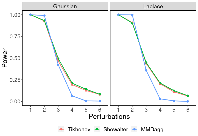
(a)

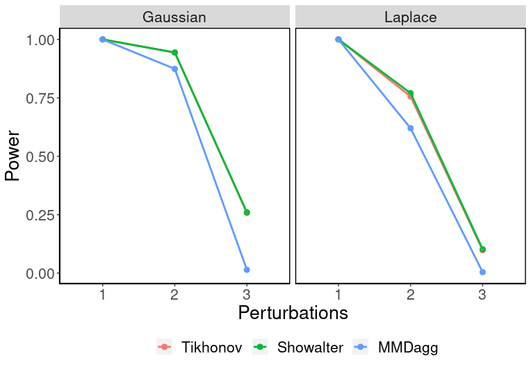
(b)

Figure 1: Power for perturbed uniform distributions. (a) $d=1$, $N=M=500$, (b) $d=2$, $N=M=2000$.

5.1.2 MNIST dataset

Next, we investigate the performance of the regularized test on the MNIST dataset (LeCun et al., 2010), which is a collection of images of digits from $0$–$9$. In our experiments, as in (Schrab et al., 2021), the images were downsampled to $7\times 7$ and consider 500 samples drawn with replacement from set $P$ while testing against the set $Q_{i}$ for $i=1,2,3,4,5$, where $P$ consists of images of the digits

$$P:0,1,2,3,4,5,67,8,9,$$

and

$$Q_{1}:1,3,5,7,9,\qquad Q_{2}:0,1,3,5,7,9,\qquad Q_{3}:0,1,2,3,5,7,9,$$

$$Q_{4}:0,1,2,3,4,5,7,9,\qquad Q_{5}:0,1,2,3,4,5,6,7,9.$$

Figure 2(a) shows the power of our test for both Gaussian and Laplace kernels in comparison to that of MMDAgg (specifically MMDAgg centered in the case of Gaussian, and MMDAgg decreasing in case of Laplace), where we set $\lambda_{L}=10^{-6}$, $\lambda_{U}=1$ for our method, and choose the bandwidth to be $h=h_{m}$ for both the kernels. Similar to Figure 1, Figure 2(a) also shows the superior performance of the regularized test over MMDAgg, particularly in the difficult cases, i.e., distinguishing between $P$ and $Q_{i}$ for larger $i$.

5.1.3 Directional data

In this part, we consider a multivariate von Mises-Fisher distribution (which is the Gaussian analogue on unit-sphere) given by $f(x,\mu,k)=\frac{k^{d/2-1}}{2\pi^{d/2}I_{d/2-1}(k)}\exp(k\mu^{T}x),\,x\in S^{d-1},$ where $k\geq 0$ is the concentration parameter and $\mu$ is the mean parameter. Figure 2(b) shows the results for testing von Mises-Fisher distribution against spherical uniform distribution ($k=0$) for different concentration parameters using a Gaussian kernel with bandwidth $h_{m}$ and $d=100$. Note that the theoretical properties of MMDAgg do not hold in this case, unlike the proposed test.

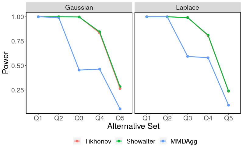
(a)

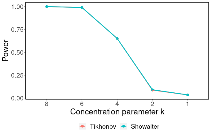
(b)

Figure 2: (a) Power for MNIST dataset using $N=M=500$. (b) Power for von Mises-Fisher distribution with different concentration parameters $k$ using $N=M=600$ and Gaussian kernel with bandwidth $h_{m}$.

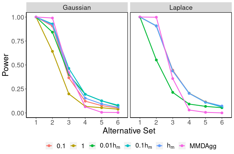
(a)

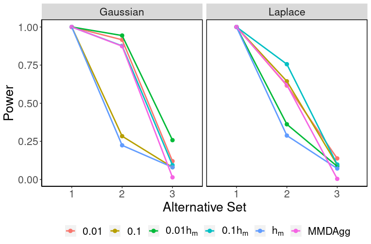
(b)

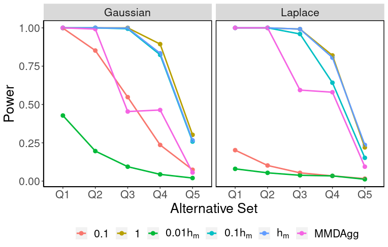
(c)

Figure 3: Power with different kernel bandwidths. (a) Perturbed uniform distribution with $d=1$, (b) Perturbed uniform distribution with $d=2$, (c) MNIST data using $N=M=500$.

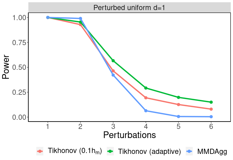
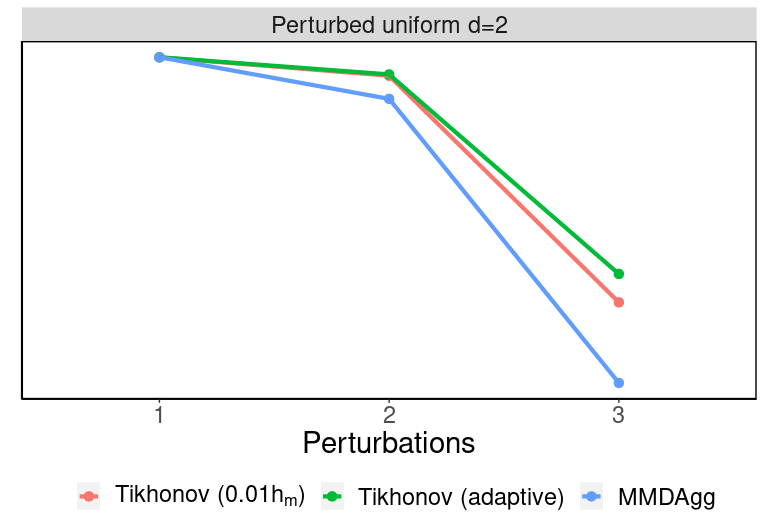
Figure 4: Power for perturbed uniform distributions using adaptive kernel bandwidth

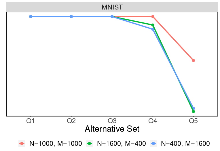
Figure 5: Power for 1-dimensional perturbed uniform distributions and MNIST data using $N+M=2000$

5.2 Effect of kernel bandwidth

While the results of the previous section dealt with a particular choice of bandwidth for the Gaussian and Laplacian kernels, in this section, we investigate the effect of kernel bandwidth on the performance of the regularized test. Figure 3 shows the performance of the test under different choices of bandwidth, wherein we used both fixed bandwidth choices and bandwidths that are multiples of the median $h_{m}$. The results in Figures 3(a,b) are obtained using the perturbed uniform distribution data with $d=1$ and $d=2$, respectively while Figure 3(c) is obtained using the MNIST data with $N=M=500$—basically using the same settings of Sections 5.1.1 and 5.1.2. We observe from Figures 3(a,b) that the performance is better at smaller bandwidths for the Gaussian kernel and deteriorates as the bandwidth gets too large, while a too-small or too-large bandwidth affects the performance in the case of a Laplacian kernel. In Figure 3(c), we can observe that the performance gets better for large bandwidth and deteriorates when the bandwidth gets too small. Thus, it seems the performance is affected by how the bandwidth is chosen, however, in all cases trying $0.01h_{m}$, $0.1h_{m}$ and $h_{m}$ always seem to yield good performance among them. Moreover, one can see from the results that for most choices of the bandwidth, the test based on $\hat{\eta}_{\lambda}$ still yields a non-trivial power as the number of perturbations (or the index of $Q_{i}$ in the case of the MNIST data) increases and eventually outperforms the MMDAgg test.

As discussed in Section 4.5, a more natural way to choose the bandwidth is to do it adaptively by taking the union of tests jointly over $\lambda\in\Lambda$ and $h\in W$. Let $\hat{\eta}_{\lambda,h}$ be the test statistic based on $\lambda$ and bandwidth $h$. We reject $H_{0}$ if $\hat{\eta}_{\lambda,h}\geq\hat{q}_{1-\frac{w\alpha}{|\Lambda||W|}}^{B,\lambda,h}$ for any $(\lambda,h)\in\Lambda\times W$. We performed such a test for $W=\{0.01h_{m},0.1h_{m},h_{m}\}$ and the results are reported in Figure 4 for the case of perturbed uniform experiments with $d=1,2$ using the Gaussian kernel. As expected, this approach gives better performance than that of fixing the bandwidth, since the test chooses the best bandwidth in $W$ for each of 500 iterations in contrast to just fixing the choice for all iterations.

5.3 Unbalanced size for $N$ and $M$

We investigated the performance of the regularized test when $N\neq M$ and report the results in Figure 5 for the 1-dimensional perturbed uniform and MNIST data set using Gaussian kernel and for fixed $N+M=2000$. It can be observed that the best performance is for $N=M=1000$ as we get more representative samples from both of the distributions $P$ and $Q$, which is also expected theoretically, as otherwise the rates are controlled by $\text{min}(M,N)$.

6 Discussion

To summarize, we have proposed a two-sample test based on spectral regularization that not only uses the mean element information like the MMD test but also uses the information about the covariance operator and showed it to be minimax optimal w.r.t. the class of local alternatives $\mathcal{P}$ defined in (4). This test improves upon the MMD test in terms of the separation rate as the MMD test is shown to be not optimal w.r.t. $\mathcal{P}$. We also presented a permutation version of the proposed regularized test along with adaptation over the regularization parameter, $\lambda$, and the kernel $K$ so that the resultant test is completely data-driven. Through numerical experiments, we also established the superiority of the proposed method over the MMD variant.

However, still there are some open questions that may be of interest to address. (i) The proposed test is computationally intensive and scales as $O((N+M)s^{2})$ where $s$ is the number of samples used to estimate the covariance operator after sample splitting. Various approximation schemes like random Fourier features (Rahimi and Recht, 2008), Nyström method (e.g., Williams and Seeger 2001; Drineas and Mahoney 2005) or sketching (Yang et al., 2017) are known to speed up the kernel methods, i.e., computationally efficient tests can be constructed using any of these approximation methods. The question of interest, therefore, is about the computational vs. statistical trade-off of these approximate tests, i.e., are these computationally efficient tests still minimax optimal w.r.t. $\mathcal{P}$? (ii) The construction of the proposed test statistic requires sample splitting, which helps in a convenient analysis. It is of interest to develop an analysis for the kernel version of Hotelling $T^{2}$-statistic (see Harchaoui et al. 2007) which does not require sample splitting. We conjecture that the theoretical results of Hotelling $T^{2}$-statistic will be similar to those of this paper, however, it may enjoy a better empirical performance but at the cost of higher computational complexity. (iii) The adaptive test presented in Section 4.5 only holds for the class of kernels, $\mathcal{K}$ for which $|\mathcal{K}|<\infty$. It will be interesting to extend the analysis for $\mathcal{K}$ for which $|\mathcal{K}|=\infty$, e.g., the class of Gaussian kernels with bandwidth in $(0,\infty)$, or the class of convex combination of certain base kernels as explained in Section 4.5.

7 Proofs

In this section, we present the proofs of all the main results of this paper.

7.1 Proof of Theorem 1

Define $a(x)=K(\cdot,x)-\mu_{P}$, and $b(x)=K(\cdot,x)-\mu_{Q}$. Then we have

$$\hat{D}_{\mathrm{MMD}}^{2} \stackrel{{\scriptstyle(*)}}{{=}}\frac{1}{N(N-1)}\sum_{i\neq j}\left\langle a(X_{i}),a(X_{j})\right\rangle_{\mathscr{H}}+\frac{1}{M(M-1)}\sum_{i\neq j}\left\langle a(Y_{i}),a(Y_{j})\right\rangle_{\mathscr{H}}$$

$$\qquad\qquad-\frac{2}{NM}\sum_{i,j}\left\langle a(X_{i}),a(Y_{j})\right\rangle_{\mathscr{H}}$$

$$\stackrel{{\scriptstyle({\dagger})}}{{=}}\frac{1}{N(N-1)}\sum_{i\neq j}\left\langle a(X_{i}),a(X_{j})\right\rangle_{\mathscr{H}}+\frac{1}{M(M-1)}\sum_{i\neq j}{\left\langle b(Y_{i}),b(Y_{j})\right\rangle}_{\mathscr{H}}$$

$$\qquad\qquad+\frac{2}{M}\sum_{i=1}^{M}{\left\langle b(Y_{i}),(\mu_{Q}-\mu_{P})\right\rangle}_{\mathscr{H}}+D_{\mathrm{MMD}}^{2}-\frac{2}{NM}\sum_{i,j}{\left\langle a(X_{i}),b(Y_{j})\right\rangle}_{\mathscr{H}}$$

$$\qquad\qquad-\frac{2}{N}\sum_{i=1}^{N}{\left\langle a(X_{i}),(\mu_{Q}-\mu_{P})\right\rangle}_{\mathscr{H}},$$

where $(*)$ follows from Lemma A.2 by setting $g_{\lambda}(x)=1$ and $({\dagger})$ follows by writing $a(Y)=b(Y)+(\mu_{Q}-\mu_{P})$ in the last two terms. Thus we have

$$\hat{D}_{\mathrm{MMD}}^{2}-D_{\mathrm{MMD}}^{2} =\leavevmode\hbox to12.54pt{\vbox to12.54pt{\text{[drawing]}}}+\leavevmode\hbox to12.54pt{\vbox to12.54pt{\text{[drawing]}}}+\leavevmode\hbox to12.54pt{\vbox to12.54pt{\text{[drawing]}}}-\leavevmode\hbox to12.54pt{\vbox to12.54pt{\text{[drawing]}}}-\leavevmode\hbox to12.54pt{\vbox to12.54pt{\text{[drawing]}}},$$

where $\leavevmode\hbox to12.54pt{\vbox to12.54pt{\text{[drawing]}}}:=\frac{1}{N(N-1)}\sum_{i\neq j}\left\langle a(X_{i}),a(X_{j})\right\rangle_{\mathscr{H}}$, $\leavevmode\hbox to12.54pt{\vbox to12.54pt{\text{[drawing]}}}:=\frac{1}{M(M-1)}\sum_{i\neq j}\left\langle b(Y_{i}),b(Y_{j})\right\rangle_{\mathscr{H}}$,

$$\leavevmode\hbox to12.54pt{\vbox to12.54pt{\text{[drawing]}}}:=\frac{2}{M}\sum_{i=1}^{M}{\left\langle b(Y_{i}),(\mu_{Q}-\mu_{P})\right\rangle}_{\mathscr{H}},\,\leavevmode\hbox to12.54pt{\vbox to12.54pt{\text{[drawing]}}}:=\frac{2}{NM}\sum_{i,j}\left\langle a(X_{i}),b(Y_{j})\right\rangle_{\mathscr{H}},$$

and $\leavevmode\hbox to12.54pt{\vbox to12.54pt{\text{[drawing]}}}:=\frac{2}{N}\sum_{i=1}^{N}{\left\langle a(X_{i}),(\mu_{Q}-\mu_{P})\right\rangle}_{\mathscr{H}}$. Next, we bound the terms – as follows (similar to the technique in the proofs of Lemmas A.4, A.5, A.6):

$$\mathbb{E}\left(\leavevmode\hbox to12.54pt{\vbox to12.54pt{\text{[drawing]}}}^{2}\right)\leq\frac{4}{N^{2}}\left\|\Sigma_{P}\right\|_{\mathcal{L}^{2}(\mathscr{H})}^{2},\qquad\mathbb{E}\left(\leavevmode\hbox to12.54pt{\vbox to12.54pt{\text{[drawing]}}}^{2}\right)\leq\frac{4}{M^{2}}\left\|\Sigma_{Q}\right\|_{\mathcal{L}^{2}(\mathscr{H})}^{2},$$

$$\mathbb{E}\left(\leavevmode\hbox to12.54pt{\vbox to12.54pt{\text{[drawing]}}}^{2}\right)\leq\frac{4}{M}\left\|\Sigma_{Q}\right\|_{\mathcal{L}^{\infty}(\mathscr{H})}\left\|\mu_{P}-\mu_{Q}\right\|_{\mathscr{H}}^{2},\quad\mathbb{E}\left(\leavevmode\hbox to12.54pt{\vbox to12.54pt{\text{[drawing]}}}^{2}\right)\leq\frac{4}{N}\left\|\Sigma_{P}\right\|_{\mathcal{L}^{\infty}(\mathscr{H})}\left\|\mu_{P}-\mu_{Q}\right\|_{\mathscr{H}}^{2},\quad\text{and}$$

$$\mathbb{E}\left(\leavevmode\hbox to12.54pt{\vbox to12.54pt{\text{[drawing]}}}^{2}\right) \leq\frac{4}{NM}{\left\langle\Sigma_{P},\Sigma_{Q}\right\rangle}_{\mathscr{H}}\leq\frac{4}{NM}\left\|\Sigma_{P}\right\|_{\mathscr{H}}\left\|\Sigma_{Q}\right\|_{\mathscr{H}}.$$

Combining these bounds with the fact that $\sqrt{ab}\leq\frac{a}{2}+\frac{b}{2}$, and that $(\sum_{i=1}^{k}a_{k})^{2}\leq k\sum_{i=1}^{k}a_{k}^{2}$ for any $a,b,a_{k}\in\mathbb{R}$, $k\in\mathbb{N}$ yields that

$$\mathbb{E}[(\hat{D}_{\mathrm{MMD}}^{2}-D_{\mathrm{MMD}}^{2})^{2}]\lesssim\frac{1}{N^{2}}+\frac{1}{M^{2}}+\frac{D_{\mathrm{MMD}}^{2}}{N}+\frac{D_{\mathrm{MMD}}^{2}}{M}\stackrel{{\scriptstyle(*)}}{{\lesssim}}\frac{1}{(N+M)^{2}}+\frac{D_{\mathrm{MMD}}^{2}}{N+M},$$ (14)

where $(*)$ follows from Lemma A.13.

When $P=Q$, we have $D_{\mathrm{MMD}}^{2}=0$. Therefore under $H_{0}$,

$$\mathbb{E}[(\hat{D}_{\mathrm{MMD}}^{2})^{2}]\lesssim\frac{1}{(N+M)^{2}}.$$ (15)

Thus using (15) and Chebyshev’s inequality yields

$$P_{H_{0}}\{\hat{D}_{\mathrm{MMD}}^{2}\geq\gamma\}\leq\alpha,$$

where $\gamma=\frac{a}{\sqrt{\alpha}(M+N)}$, for some constant $a>0$.

Next, we can use the bound in (14) to bound the power. Let $\gamma_{1}=\frac{1}{\sqrt{\delta}(N+M)}+\frac{\sqrt{D_{\mathrm{MMD}}^{2}}}{\sqrt{\delta}\sqrt{N+M}}$. Then

$$P_{H_{1}}\{\hat{D}_{\mathrm{MMD}}^{2}\geq\gamma\} \stackrel{{\scriptstyle(*)}}{{\geq}}P_{H_{1}}\{\hat{D}_{\mathrm{MMD}}^{2}>D_{\mathrm{MMD}}^{2}-\gamma_{1}\}$$

$$\geq P_{H_{1}}\{|\hat{D}_{\mathrm{MMD}}^{2}-D_{\mathrm{MMD}}^{2}|\leq\gamma_{1}\}\stackrel{{\scriptstyle(**)}}{{\geq}}1-\delta,$$

where $(*)$ holds when $D_{\mathrm{MMD}}^{2}\geq\gamma+\gamma_{1}$, which is implied if $D_{\mathrm{MMD}}^{2}\gtrsim\frac{1}{N+M}$, which in turn is implied if $\left\|u\right\|_{L^{2}(R)}^{2}\gtrsim(N+M)^{\frac{-2\theta}{2\theta+1}},$ where in the last implication we used Lemma A.19. $(**)$ follows from (14) and an application of Chebyshev’s inequality. The desired result, therefore, holds by taking infimum over $(P,Q)\in\mathcal{P}$.

Finally, we will show that we cannot achieve a rate better than $(M+N)^{\frac{-2\theta}{2\theta+1}}$ over $\mathcal{P}$. To this end, let $R$ be a probability measure. Recall that $\mathcal{T}=\sum_{i\in I}\lambda_{i}\tilde{\phi_{i}}\otimes_{L^{2}(R)}\tilde{\phi_{i}}$. Let $\bar{\phi_{i}}=\phi_{i}-\mathbb{E}_{R}\phi_{i}$, where $\phi_{i}=\frac{\mathfrak{I}^{*}\tilde{\phi_{i}}}{\lambda_{i}}$. Then $\mathfrak{I}\bar{\phi_{i}}=\mathfrak{I}\phi_{i}=\frac{\mathcal{T}\tilde{\phi}_{i}}{\lambda_{i}}=\tilde{\phi_{i}}.$ Assuming $\lambda_{i}=h(i)$, where $h$ is an invertible, continuous function (for example $h=i^{-\beta}$, $h=e^{-\tau i}$ corresponds to polynomial decay and exponential decay respectively), let $k=\lfloor h^{-1}((N+M)^{\frac{-1}{2\theta+1}})\rfloor$, hence $\lambda_{k}=(N+M)^{\frac{-1}{2\theta+1}}$. Define

$$f:=b\bar{\phi}_{k},$$

where $b<\sqrt{\frac{a}{4\sqrt{\alpha}}}$. Then $\left\|f\right\|_{L^{2}(R)}^{2}=b^{2}\lesssim 1,$ and thus $f\in L^{2}(R)$. Define

$$\tilde{u}:=\mathcal{T}^{\theta}f=b\lambda_{k}^{\theta}\tilde{\phi}_{k},\quad\text{and}\quad u:=b\lambda_{k}^{\theta}\bar{\phi}_{k}.$$

Note that $\mathbb{E}_{R}u=b\lambda^{\theta}_{k}\mathbb{E}_{R}\bar{\phi_{k}}=0$. Since $\mathfrak{I}u=\tilde{u}$, we have $u\in[\tilde{u}]_{\sim}\in\text{Ran}(\mathcal{T}^{\theta}),$ $\left\|u\right\|_{L^{2}(R)}^{2}=b^{2}\lambda_{k}^{2\theta}>\Delta_{N,M},$ and $|u(x)|\leq|2b\sup_{k}\left\|\phi_{k}\right\|_{\infty}(N+M)^{\frac{-\theta}{2\theta+1}}|\leq 1$, for $N+M$ large enough. This implies that we can find $(P,Q)\in\mathcal{P}$ such that $\frac{dP}{dR}=u+1$ and $\frac{dQ}{dR}=2-\frac{dP}{dR}.$ Then for such $(P,Q)$, we have $D^{2}_{\mathrm{MMD}}=4\left\|\mathcal{T}^{1/2}u\right\|_{L^{2}(R)}^{2}=4b^{2}\lambda_{k}^{2\theta+1}=\frac{4b^{2}}{(N+M)}<\frac{a}{\sqrt{\alpha}(N+M)}=\gamma$. Therefore there exists some $\varepsilon>0$ such that $D^{2}_{\mathrm{MMD}}<\gamma-\varepsilon.$ Hence, we have

$$P_{H_{1}}\{\hat{D}_{\mathrm{MMD}}^{2}\geq\gamma\} <P_{H_{1}}\{\hat{D}_{\mathrm{MMD}}^{2}\geq D_{\mathrm{MMD}}^{2}+\varepsilon\}<P_{H_{1}}\{|\hat{D}_{\mathrm{MMD}}^{2}-D_{\mathrm{MMD}}^{2}|\geq\varepsilon\}$$

$$\stackrel{{\scriptstyle(*)}}{{\lesssim}}\frac{1}{\varepsilon^{2}(N+M)^{2}}\leq\delta,$$

where in $(*)$ we used (14) along with Chebyshev’s inequality, and the last inequality holds for $N+M>\frac{1}{\varepsilon\sqrt{\delta}}.$

7.2 Proof of Theorem 2

Let $\phi(X_{1},\dots,X_{N},Y_{1},\dots,Y_{M})$ be any test that rejects $H_{0}$ when $\phi=1$ and fail to reject when $\phi=0$. Fix some probability probability measure $R$, and let $\{(P_{k},Q_{k})\}^{L}_{k=1}\subset\mathcal{P}$ such that $P_{k}+Q_{k}=2R$. First, we prove the following lemma.

Lemma 7.1.

For $0<\delta<1-\alpha$, if the following hold,

$$\mathbb{E}_{R^{N}}\left[\left(\frac{1}{L}\sum_{i=1}^{L}\frac{dP_{k}^{N}}{dR^{N}}\right)^{2}\right]\leq 1+(1-\alpha-\delta)^{2},$$ (16)

$$\mathbb{E}_{R^{N}}\left[\left(\frac{1}{L}\sum_{i=1}^{L}\frac{dQ_{k}^{N}}{dR^{N}}\right)^{2}\right]\leq 1+(1-\alpha-\delta)^{2},$$ (17)

then

$$R^{*}_{\Delta_{N,M}}\geq\delta.$$

Proof.

For any two-sample test $\phi(X_{1},\dots,X_{N},Y_{1},\dots,Y_{M})\in\Phi_{N,M,\alpha}$, define a corresponding one sample test as $\Psi_{Q}(X_{1},\dots,X_{N}):=\mathbb{E}_{Q^{M}}\phi(X_{1},\dots,X_{N},Y_{1},\dots,Y_{M}),$ and note that it is still an $\alpha$-level test since $Q^{N}(\{\Psi_{Q}=1\})=\mathbb{E}_{Q^{N}}[\Psi_{Q}]=\mathbb{E}_{Q^{N}\times Q^{M}}[\phi]\leq\alpha$. For any $\phi\in\Phi_{N,M,\alpha}$, we have

$$R_{\Delta_{N,M}}(\phi)=\sup_{(P,Q)\in\mathcal{P}}\mathbb{E}_{P^{N}\times Q^{M}}[1-\phi]$$

$$\geq\sup_{(P,Q)\in\mathcal{P}\ :\ P+Q=2R}\mathbb{E}_{P^{N}\times Q^{M}}[1-\phi]\geq\frac{1}{L}\sum_{k=1}^{L}\mathbb{E}_{P_{k}^{N}}[1-\Psi_{Q_{k}}]$$

$$=\frac{1}{L}\sum_{k=1}^{L}\left[P_{k}^{N}(\{\Psi_{Q_{k}}=0\})-Q_{k}^{N}(\{\Psi_{Q_{k}}=0\})+Q_{k}^{N}(\{\Psi_{Q_{k}}=0\})\right]$$

$$\geq 1-\alpha+\frac{1}{L}\sum_{k=1}^{L}\left[P_{k}^{N}(\{\Psi_{Q_{k}}=0\})-Q_{k}^{N}(\{\Psi_{Q_{k}}=0\})\right]$$

$$=\frac{1}{L}\sum_{k=1}^{L}\left[P_{k}^{N}(\{\Psi_{Q_{k}}=0\})-R^{N}(\{\Psi_{Q_{k}}=0\})\right]+\frac{1}{L}\sum_{k=1}^{L}\left[R^{N}(\{\Psi_{Q_{k}}=0\})-Q_{k}^{N}(\{\Psi_{Q_{k}}=0\})\right]$$

$$\qquad\qquad\qquad+1-\alpha$$

$$\geq 1-\alpha-\sup_{\mathcal{A}}\left|\frac{1}{L}\sum_{k=1}^{L}\left(P_{k}^{N}(\mathcal{A})-R^{N}(\mathcal{A})\right)\right|-\sup_{\mathcal{A}}\left|\frac{1}{L}\sum_{k=1}^{L}\left(R^{N}(\mathcal{A})-Q_{k}^{N}(\mathcal{A})\right)\right|$$

$$\geq 1-\alpha-\frac{1}{2}\sqrt{\mathbb{E}_{R^{N}}\left[\left(\frac{1}{L}\sum_{k=1}^{L}\frac{dP_{k}^{N}}{dR^{N}}\right)^{2}\right]-1}-\frac{1}{2}\sqrt{\mathbb{E}_{R^{N}}\left[\left(\frac{1}{L}\sum_{k=1}^{L}\frac{dQ_{k}^{N}}{dR^{N}}\right)^{2}\right]-1}\ ,$$

where the last inequality follows by noting that

$$\sup_{\mathcal{A}}\left|\frac{1}{L}\sum_{k=1}^{L}\left(P_{k}^{N}(\mathcal{A})-R^{N}(\mathcal{A})\right)\right|+\sup_{\mathcal{A}}\left|\frac{1}{L}\sum_{k=1}^{L}\left(R^{N}(\mathcal{A})-Q_{k}^{N}(\mathcal{A})\right)\right|$$

$$\stackrel{{\scriptstyle({\dagger})}}{{=}}\frac{1}{2}\left\|\frac{1}{L}\sum_{k=1}^{L}dP_{k}^{N}-dR^{N}\right\|_{1}+\frac{1}{2}\left\|dR^{N}-\frac{1}{L}\sum_{k=1}^{L}dQ_{k}^{N}\right\|_{1}$$

$$=\frac{1}{2}\mathbb{E}_{R^{N}}\left|\frac{1}{L}\sum_{k=1}^{L}\frac{dP_{k}^{N}}{dR^{N}}-1\right|+\frac{1}{2}\mathbb{E}_{R^{N}}\left|1-\frac{1}{L}\sum_{k=1}^{L}\frac{dQ_{k}^{N}}{dR^{N}}\right|$$

$$\leq\frac{1}{2}\sqrt{\mathbb{E}_{R^{N}}\left[\left(\frac{1}{L}\sum_{k=1}^{L}\frac{dP_{k}^{N}}{dR^{N}}\right)^{2}\right]-1}+\frac{1}{2}\sqrt{\mathbb{E}_{R^{N}}\left[\left(\frac{1}{L}\sum_{k=1}^{L}\frac{dQ_{k}^{N}}{dR^{N}}\right)^{2}\right]-1},$$

where $({\dagger})$ uses the alternative definition of total variation distance using the $L_{1}$-distance. Thus taking the infimum over $\phi\in\Phi_{N,M,\alpha}$ yields

$$R^{*}_{\Delta_{N,M}}\geq 1-\alpha-\frac{1}{2}\sqrt{\mathbb{E}_{R^{N}}\left[\left(\frac{1}{L}\sum_{k=1}^{L}\frac{dP_{k}^{N}}{dR^{N}}\right)^{2}\right]-1}-\frac{1}{2}\sqrt{\mathbb{E}_{R^{N}}\left[\left(\frac{1}{L}\sum_{k=1}^{L}\frac{dQ_{k}^{N}}{dR^{N}}\right)^{2}\right]-1}$$

and the result follows. ∎

Thus, in order to show that a separation boundary $\Delta_{N,M}$ will imply that $R^{*}_{\Delta_{N,M}}\geq\delta$, it is sufficient to find a set of distributions $\{(P_{k},Q_{k})\}_{k}$ such that (16) and (17) hold. Note that since $P_{k}+Q_{k}=2R$, it is clear that the operator $\mathcal{T}$ is fixed for all $k\in\{1,\dots,L\}$. Recall $\mathcal{T}=\sum_{i\in I}\lambda_{i}\tilde{\phi_{i}}\otimes_{L^{2}(R)}\tilde{\phi_{i}}$. Let $\bar{\phi_{i}}=\phi_{i}-\mathbb{E}_{R}\phi_{i}$, where $\phi_{i}=\frac{\mathfrak{I}^{*}\tilde{\phi_{i}}}{\lambda_{i}}$. Then $\mathfrak{I}\bar{\phi_{i}}=\mathfrak{I}\phi_{i}=\frac{\mathcal{T}\tilde{\phi}_{i}}{\lambda_{i}}=\tilde{\phi_{i}}$. Furthermore, since the lower bound on $R^{*}_{\Delta_{N,M}}$ is only in terms of $N$, for simplicity, we will write $\Delta_{N,M}$ as $\Delta_{N}$. However, since we assume $M\leq N\leq DM$, we can write the resulting bounds in terms of $(N+M)$ using Lemma A.13.

Following the ideas from Ingster (1987) and Ingster (1993), we now provide the proof of Theorem 2.

Polynomial decay (Case I): $\lambda_{i}\asymp i^{-\beta}$, $\beta>1$, $\sup_{i}\left\|\phi_{i}\right\|_{\infty}<\infty$ and $\theta\geq\frac{1}{4\beta}$.

Let

$$B_{N}=\left\lfloor\frac{\Delta_{N}^{-1/2\theta\beta}}{16(\sup_{i}\left\|\phi_{i}\right\|_{\infty})^{2}}\right\rfloor,$$

$C_{N}=\lfloor\sqrt{B_{N}}\rfloor$ and $a_{N}=\sqrt{\frac{\Delta_{N}}{C_{N}}}$. For $k\in\{1,\dots,L\}$, define

$$f_{N,k}:=a_{N}\sum_{i=1}^{B_{N}}\varepsilon_{ki}\lambda_{i}^{-\theta}\bar{\phi_{i}},$$

where $\varepsilon_{k}:=\{\varepsilon_{k1},\varepsilon_{k2},\ldots,\varepsilon_{kB_{N}}\}\in\{0,1\}^{B_{N}}$ such that $\sum_{i=1}^{B_{N}}\varepsilon_{ki}=C_{N}$, thus $L={B_{N}\choose C_{N}}$. Then we have $\left\|f_{N,k}\right\|^{2}_{L^{2}(R)}=a_{N}^{2}\sum_{i=1}^{B_{N}}\lambda_{i}^{-2\theta}\varepsilon_{ki}^{2}\lesssim a_{N}^{2}B_{N}^{2\theta\beta}C_{N}=\Delta_{N}B_{N}^{2\theta\beta}\lesssim 1$, and thus $f_{N,k}\in L^{2}(R)$. Define

$$\tilde{u}_{N,k}:=\mathcal{T}^{\theta}f_{N,k}=a_{N}\sum_{i=1}^{B_{N}}\lambda_{i}^{\theta}{\left\langle\varepsilon_{ki}\lambda_{i}^{-\theta}\bar{\phi_{i}},\tilde{\phi_{i}}\right\rangle}_{L^{2}(R)}\tilde{\phi_{i}}=a_{N}\sum_{i=1}^{B_{N}}\varepsilon_{ki}\tilde{\phi_{i}},$$

and

$$u_{N,k}:=a_{N}\sum_{i=1}^{B_{N}}\varepsilon_{ki}\bar{\phi_{i}}.$$

Note that $\mathbb{E}_{R}u_{N,k}=a_{N}\sum_{i=1}^{B_{N}}\varepsilon_{ki}\mathbb{E}_{R}\bar{\phi_{i}}=0$. Since $\mathfrak{I}u_{N,k}=\tilde{u}_{N,k}$, we have $u_{N,k}\in[\tilde{u}_{N,k}]_{\sim}\in\text{Ran}(\mathcal{T}^{\theta})$, $\left\|u_{N,k}\right\|_{L^{2}(R)}^{2}=a_{N}^{2}C_{N}=\Delta_{N},$ and

$$|u_{N,k}(x)| \leq 2a_{N}\sum_{i=1}^{B_{N}}\varepsilon_{ki}\left\|\phi_{i}\right\|_{\infty}\leq 2a_{N}C_{N}\sup_{i}\left\|\phi_{i}\right\|_{\infty}=2\sqrt{\Delta_{N}C_{N}}\sup_{i}\left\|\phi_{i}\right\|_{\infty}\leq\Delta_{N}^{\frac{1}{2}-\frac{1}{8\theta\beta}}\leq 1,$$

where the last inequality follows by using $\theta\geq\frac{1}{4\beta}.$ This implies that we can find $(P_{k},Q_{k})\in\mathcal{P}$ such that $\frac{dP_{k}}{dR}=u_{N,k}+1$ and $\frac{dQ_{k}}{dR}=2-\frac{dP_{k}}{dR}$. Thus it remains to verify conditions (16) and (17) from Lemma 7.1.

For condition (16), we have

$$\mathbb{E}_{R^{N}}\left[\left(\frac{1}{L}\sum_{k=1}^{L}\frac{dP_{k}^{N}}{dR^{N}}\right)^{2}\right]=\mathbb{E}_{R^{N}}\left[\left(\frac{1}{L}\sum_{k=1}^{L}\prod_{j=1}^{N}(u_{N,k}(X_{j})+1)\right)^{2}\right]$$

$$=\mathbb{E}_{R^{N}}\left[\frac{1}{L}\sum_{k=1}^{L}\prod_{j=1}^{N}\left(1+a_{N}\sum_{i=1}^{B_{N}}\varepsilon_{ki}\bar{\phi_{i}}(X_{j})\right)\right]^{2}$$

$$=\frac{1}{L^{2}}\sum_{k,k^{\prime}=1}^{L}\prod_{j=1}^{N}\left(1+a_{N}\sum_{i=1}^{B_{N}}\varepsilon_{ki}\mathbb{E}_{R}\bar{\phi_{i}}(X_{j})\right.$$

$$\qquad\qquad\qquad\left.+a_{N}\sum_{i=1}^{B_{N}}\varepsilon_{k^{\prime}i}\mathbb{E}_{R}\bar{\phi_{i}}(X_{j})+a_{N}^{2}\sum_{i,l=1}^{B_{N}}\varepsilon_{ki}\varepsilon_{k^{\prime}l}\mathbb{E}_{R}[\bar{\phi_{i}}(X_{j})\bar{\phi_{l}}(X_{j})]\right)$$

$$\stackrel{{\scriptstyle({\dagger})}}{{\leq}}\frac{1}{L^{2}}\sum_{k,k^{\prime}=1}^{L}\left(1+a_{N}^{2}\sum_{i=1}^{B_{N}}\varepsilon_{ki}\varepsilon_{k^{\prime}i}\right)^{N},$$

where $({\dagger})$ follows from the fact that $\mathbb{E}_{R}[\bar{\phi_{i}}(X)]=0$ and $\mathbb{E}_{R}[\bar{\phi_{i}}(X)\bar{\phi_{l}}(X)]=\langle\bar{\phi}_{i},\bar{\phi}_{l}\rangle_{L^{2}(R)}=\delta_{il}$. Similarly for (17), we have

$$\mathbb{E}_{R^{N}}\left[\left(\frac{1}{L}\sum_{i=1}^{L}\frac{dQ_{k}^{N}}{dR^{N}}\right)^{2}\right]\leq\frac{1}{L^{2}}\sum_{k,k^{\prime}=1}^{L}\left(1+a_{N}^{2}\sum_{i=1}^{B_{N}}\varepsilon_{ki}\varepsilon_{k^{\prime}i}\right)^{N},$$

where $L={B_{N}\choose C_{N}}$. Thus it is sufficient to show that $\exists c(\alpha,\delta)$ such that if $\Delta_{N}\leq c(\alpha,\delta)N^{\frac{-4\theta\beta}{4\theta\beta+1}}$, then $\frac{1}{L^{2}}\sum_{k,k^{\prime}=1}^{L}(1+a_{N}^{2}\sum_{i=1}^{B_{N}}\varepsilon_{ki}\varepsilon_{k^{\prime}i})^{N}\leq 1+(1-\alpha-\delta)^{2}$. To this end, consider

$$\frac{1}{L^{2}}\sum_{k,k^{\prime}=1}^{L}\left(1+a_{N}^{2}\sum_{i=1}^{B_{N}}\varepsilon_{ki}\varepsilon_{k^{\prime}i}\right)^{N}=\frac{1}{L^{2}}{B_{N}\choose C_{N}}\sum_{i=0}^{C_{N}}{B_{N}-C_{N}\choose C_{N}-i}{C_{N}\choose i}(1+a_{N}^{2}i)^{N}$$

$$\leq\sum_{i=0}^{C_{N}}\frac{{B_{N}-C_{N}\choose C_{N}-i}{C_{N}\choose i}}{{B_{N}\choose C_{N}}}\exp(Na_{N}^{2}i)=\sum_{i=0}^{C_{N}}\frac{H_{i}}{i!}\exp(Na_{N}^{2}i),$$

where $H_{i}:=\frac{((B_{N}-C_{N})!C_{N}!)^{2}}{((C_{N}-i)!)^{2}B_{N}!(B_{N}-2C_{N}+i)!},$ then as argued in Ingster (1987), it can be shown for any $r>0$, we have $\frac{H_{i}}{H_{i-1}}\leq 1+r$ and $H_{0}\leq\exp(r-1)$, thus $H_{i}\leq\frac{(1+r)^{i}}{e}$, which yields that for any $r>0$, we have

$$\sum_{i=0}^{C_{N}}\frac{H_{i}}{i!}\exp(Na_{N}^{2}i) \leq\exp\left((1+r)\exp(N\Delta_{N}C_{N}^{-1})-1\right).$$

Since $C_{N}\asymp\Delta_{N}^{-1/4\theta\beta}$ and $\Delta_{N}\leq c(\alpha,\delta)N^{\frac{-4\theta\beta}{4\theta\beta+1}}$, we can choose $c(\alpha,\delta)$ and $r$ such that

$$\exp\left((1+r)\exp(N\Delta_{N}C_{N}^{-1})-1\right)\leq 1+(1-\alpha-\delta)^{2}$$

and therefore both (16) and (17) hold.

Polynomial decay (Case II): $\lambda_{i}\asymp i^{-\beta}$, $\beta>1$, $\theta\geq\frac{1}{2}$ and $\sup_{i}\left\|\phi_{i}\right\|_{\infty}$ is not finite.

Since $\lambda_{i}\asymp i^{-\beta}$, $\beta>1$, there exists constants $\underline{A}>0$ and $\bar{A}>0$ such that $\underline{A}i^{-\beta}\leq\lambda_{i}\leq\bar{A}i^{-\beta}$. Let $B_{N}=\lfloor\left(\frac{\underline{A}\Delta_{N}^{-1}}{4\kappa}\right)^{\frac{1}{2\theta\beta}}\rfloor$, $C_{N}=\lfloor\sqrt{B_{N}}\rfloor$ and $a_{N}=\sqrt{\frac{\Delta_{N}}{C_{N}}}$. The proof proceeds similarly to that of Case I by noting that

$$|u_{N,k}(x)| =\left|{\left\langle k(\cdot,x)-\mu_{R},a_{N}\sum_{i=1}^{B_{N}}\varepsilon_{ki}\phi_{i}\right\rangle}_{\mathscr{H}}\right|\leq\left\|k(\cdot,x)-\mu_{R}\right\|_{\mathscr{H}}\left\|a_{N}\sum_{i=1}^{B_{N}}\varepsilon_{ki}\phi_{i}\right\|_{\mathscr{H}}$$

$$\leq 2\sqrt{\kappa}\left\|a_{N}\sum_{i=1}^{B_{N}}\varepsilon_{ki}\phi_{i}\right\|_{\mathscr{H}}\stackrel{{\scriptstyle(*)}}{{\leq}}1,$$

where $(*)$ follows from

$$\left\|a_{N}\sum_{i=1}^{B_{N}}\varepsilon_{ki}\phi_{i}\right\|_{\mathscr{H}}^{2} =a_{N}^{2}\sum_{i,j=1}^{B_{N}}\varepsilon_{ki}\varepsilon_{kj}{\left\langle\phi_{i},\phi_{j}\right\rangle}_{\mathscr{H}}=a_{N}^{2}\sum_{i,j=1}^{B_{N}}\lambda_{i}^{-1}\varepsilon_{ki}\varepsilon_{kj}{\left\langle\tilde{\phi_{i}},\tilde{\phi_{j}}\right\rangle}_{L^{2}(R)}$$

$$=a_{N}^{2}\sum_{i=1}^{B_{N}}\lambda_{i}^{-1}\varepsilon_{ki}^{2}\leq a_{N}^{2}\underline{A}^{-1}B_{N}^{\beta}C_{N}=\Delta_{N}\underline{A}^{-1}B_{N}^{\beta}\stackrel{{\scriptstyle({\dagger})}}{{\leq}}\Delta_{N}\underline{A}^{-1}B_{N}^{2\theta\beta}=\frac{1}{4\kappa},$$

where $({\dagger})$ follows using $\theta\geq 1/2$. Then the rest of the proof proceeds exactly similar to Case I.

Exponential decay: $\lambda_{i}\asymp e^{-\tau i}$, $\tau>0$.

Since $\lambda_{i}\asymp e^{-\tau i}$, $\tau>0$, there exists constants $\underline{A}>0$ and $\bar{A}>0$ such that $\underline{A}e^{-\tau i}\leq\lambda_{i}\leq\bar{A}e^{-\tau i}$. Let $B_{N}=\lfloor(2\tau\max\{\theta,\frac{1}{2}\})^{-1}\log(\frac{\underline{A}}{4\kappa\Delta_{N}})\rfloor$, $C_{N}=\lfloor\sqrt{B_{N}}\rfloor$ and $a_{N}=\sqrt{\frac{\Delta_{N}}{C_{N}}}$, where $\theta>0$. Then similar to the previous cases, define

$$f_{N,k}:=a_{N}\sum_{i=1}^{B_{N}}\varepsilon_{ki}\lambda_{i}^{-\theta}\bar{\phi_{i}}$$

so that $\left\|f_{N,k}\right\|^{2}_{L^{2}(R)}=a_{N}^{2}\sum_{i=1}^{B_{N}}\lambda_{i}^{-2\theta}\varepsilon_{ki}^{2}\lesssim a_{N}^{2}e^{2\tau\theta B_{N}}C_{N}\lesssim\Delta_{N}e^{2\tau\theta B_{N}}\lesssim 1$, and thus $f_{N,k}\in L^{2}(R)$. As in the previous cases, define $u_{N,k}:=a_{N}\sum_{i=1}^{B_{N}}\varepsilon_{ki}\bar{\phi_{i}},$ so that $\left\|u_{N,k}\right\|^{2}_{L^{2}(R)}=a_{N}^{2}C_{N}=\Delta_{N}.$ As in Case II, it is easy to verify that

$$|u_{N,k}(x)|\leq 2\sqrt{\kappa}\left\|a_{N}\sum_{i=1}^{B_{N}}\varepsilon_{ki}\phi_{i}\right\|_{\mathscr{H}}\stackrel{{\scriptstyle(*)}}{{\leq}}1,$$

where $(*)$ follows from

$$\left\|a_{N}\sum_{i=1}^{B_{N}}\varepsilon_{ki}\phi_{i}\right\|_{\mathscr{H}}^{2} =a_{N}^{2}\sum_{i,j=1}^{B_{N}}\varepsilon_{ki}\varepsilon_{kj}{\left\langle\phi_{i},\phi_{j}\right\rangle}_{\mathscr{H}}=a_{N}^{2}\sum_{i,j=1}^{B_{N}}\lambda_{i}^{-1}\varepsilon_{ki}\varepsilon_{kj}{\left\langle\tilde{\phi_{i}},\tilde{\phi_{j}}\right\rangle}_{L^{2}(R)}$$

$$=a_{N}^{2}\sum_{i=1}^{B_{N}}\lambda_{i}^{-1}\varepsilon_{ki}^{2}\leq a_{N}^{2}\underline{A}^{-1}e^{\tau B_{N}}C_{N}=\Delta_{N}\underline{A}^{-1}e^{\tau B_{N}}\leq\frac{1}{4\kappa}.$$

Thus it just remains to verify (16) and (17). As shown in Case I, we will have

$$\sum_{i=0}^{C_{N}}\frac{H_{i}}{i!}\exp(Na_{N}^{2}i) \leq\exp\left((1+r)\exp(N\Delta_{N}C_{N}^{-1})-1\right).$$

Since $C_{N}=d_{\theta}\sqrt{\log\frac{a}{\Delta_{N}}}$, where $a=\frac{\underline{A}}{4\kappa}$, $d_{\theta}=\sqrt{2\tau\max\{\theta,1/2\}}$, and $\Delta_{N}\leq c(\alpha,\delta,\theta)\frac{(\log N)^{b}}{N}$ for $b<\frac{1}{2}$, this yields that

$$\exp\left((1+r)\exp(N\Delta_{N}C_{N}^{-1})-1\right)\leq\exp\left((1+r)\exp\left(\frac{c(\alpha,\delta,\theta)(\log N)^{b}}{d_{\theta}\sqrt{\log\left(\frac{aN}{c(\alpha,\delta,\theta)(\log N)^{b}}\right)}}\right)-1\right).$$

Thus for large enough $N$, we can choose $c(\alpha,\delta,\theta)$ and $r$ such that

$$\exp\left((1+r)\exp(N\Delta_{N}C_{N}^{-1})-1\right)\leq 1+(1-\alpha-\delta)^{2}.$$

Therefore, both (16) and (17) hold.

7.3 Proof of Theorem 3

Define

$$S_{z}:\mathscr{H}\to\mathbb{R}^{s},\ \ f\to\frac{1}{\sqrt{s}}(f(Z_{1}),\cdot\cdot\cdot,f(Z_{s}))^{\top}$$

so that

$$S_{z}^{*}:\mathbb{R}^{s}\to\mathscr{H},\ \ \alpha\to\frac{1}{\sqrt{s}}\sum_{i=1}^{s}\alpha_{i}K(\cdot,Z_{i}).$$

It can be shown that $\hat{\Sigma}_{PQ}=S_{z}^{*}\tilde{\boldsymbol{H}}_{s}S_{z}$ (Sterge and Sriperumbudur, 2022, Proposition C.1). Also, it can be shown that if $(\hat{\lambda}_{i},\hat{\alpha_{i}})_{i}$ is the eigensystem of $\frac{1}{s}\tilde{\boldsymbol{H}_{s}}^{1/2}K_{s}\tilde{\boldsymbol{H}_{s}}^{1/2}$ where $K_{s}:=[K(Z_{i},Z_{j})]_{i,j\in[s]}$, $\boldsymbol{H}_{s}=\boldsymbol{I}_{s}-\frac{1}{s}\boldsymbol{1}_{s}\boldsymbol{1}_{s}^{\top}$, and $\tilde{\boldsymbol{H}}_{s}=\frac{s}{s-1}\boldsymbol{H}_{s}$, then $(\hat{\lambda}_{i},\hat{\phi_{i}})_{i}$ is the eigensystem of $\hat{\Sigma}_{PQ}$, where

$$\hat{\phi}_{i}=\frac{1}{\sqrt{\hat{\lambda}_{i}}}S_{z}^{*}\tilde{\boldsymbol{H}_{s}}^{1/2}\hat{\alpha_{i}}.$$ (18)

We refer the reader to (Sriperumbudur and Sterge, 2022, Proposition 1) for details. Using (18) in the definition of $g_{\lambda}(\hat{\Sigma}_{PQ})$, we have

$$g_{\lambda}(\hat{\Sigma}_{PQ}) =g_{\lambda}(0)\boldsymbol{I}+S_{z}^{*}\tilde{\boldsymbol{H}}_{s}^{1/2}\left[\sum_{i}\left(\frac{g_{\lambda}(\hat{\lambda}_{i})-g_{\lambda}(0)}{\hat{\lambda}_{i}}\right)\hat{\alpha}_{i}\hat{\alpha}_{i}^{\top}\right]\tilde{\boldsymbol{H}}_{s}^{1/2}S_{z}$$

$$=g_{\lambda}(0)\boldsymbol{I}+S_{z}^{*}\tilde{\boldsymbol{H}}_{s}^{1/2}G\tilde{\boldsymbol{H}}_{s}^{1/2}S_{z}.$$

Define $\boldsymbol{1}_{n}:=(1,\stackrel{{\scriptstyle n}}{{\ldots}},1)^{\top}$, and let $\boldsymbol{1}_{n}^{i}$ be a vector of zeros with only the $i^{th}$ entry equal one. Also we define $S_{x}$ and $S_{y}$ similar to that of $S_{z}$ based on samples $(X_{i})^{n}_{i=1}$ and $(Y_{i})^{m}_{i=1}$, respectively. Based on (Sterge and Sriperumbudur, 2022, Proposition C.1), it can be shown that $K_{s}=sS_{z}S_{z}^{*}$, $K_{n}:=nS_{x}S_{x}^{*}$, $K_{m}=mS_{y}S_{y}^{*}$, $K_{ns}=\sqrt{ns}S_{x}S_{z}^{*}$, $K_{ms}=\sqrt{ms}S_{y}S_{z}^{*}$, and $K_{mn}=\sqrt{mn}S_{y}S_{x}^{*}$.

Based on these observations, we have

$$={\left\langle g_{\lambda}(\hat{\Sigma}_{PQ})\sum_{i=1}^{n}K(\cdot,X_{i}),\sum_{j=1}^{n}K(\cdot,X_{j})\right\rangle}_{\mathscr{H}}=n{\left\langle g_{\lambda}(\hat{\Sigma}_{PQ})S_{x}^{*}\boldsymbol{1}_{n},S_{x}^{*}\boldsymbol{1}_{n}\right\rangle}_{\mathscr{H}}$$

$$=n{\left\langle S_{x}g_{\lambda}(\hat{\Sigma}_{PQ})S_{x}^{*}\boldsymbol{1}_{n},\boldsymbol{1}_{n}\right\rangle}_{2}=n{\left\langle g_{\lambda}(0)\frac{1}{n}K_{n}+\frac{1}{ns}K_{ns}\tilde{\boldsymbol{H}}_{s}^{1/2}G\tilde{\boldsymbol{H}}_{s}^{1/2}K_{ns}^{\top}\boldsymbol{1}_{n},\boldsymbol{1}_{n}\right\rangle}_{2}$$

$$=\boldsymbol{1}_{n}^{\top}\left(g_{\lambda}(0)K_{n}+\frac{1}{s}K_{ns}\tilde{\boldsymbol{H}}^{1/2}_{s}G\tilde{\boldsymbol{H}}^{1/2}_{s}K_{ns}^{\top}\right)\boldsymbol{1}_{n},$$

$$=\sum_{i=1}^{n}{\left\langle g_{\lambda}(\hat{\Sigma}_{PQ})K(\cdot,X_{i}),K(\cdot,X_{i})\right\rangle}_{\mathscr{H}}=n\sum_{i=1}^{n}{\left\langle g_{\lambda}(\hat{\Sigma}_{PQ})S_{x}^{*}\boldsymbol{1}_{n}^{i},S_{x}^{*}\boldsymbol{1}_{n}^{i}\right\rangle}_{\mathscr{H}}$$

$$=n\sum_{i=1}^{n}{\left\langle S_{x}g_{\lambda}(\hat{\Sigma}_{PQ})S_{x}^{*}\boldsymbol{1}_{n}^{i},\boldsymbol{1}_{n}^{i}\right\rangle}_{2}=n\sum_{i=1}^{n}{\left\langle g_{\lambda}(0)\frac{1}{n}K_{n}+\frac{1}{ns}K_{ns}\tilde{\boldsymbol{H}}_{s}^{1/2}G\tilde{\boldsymbol{H}}_{s}^{1/2}K_{ns}^{\top}\boldsymbol{1}_{n}^{i},\boldsymbol{1}_{n}^{i}\right\rangle}_{2}$$

$$=\text{Tr}\left(g_{\lambda}(0)K_{n}+\frac{1}{s}K_{ns}\tilde{\boldsymbol{H}}^{1/2}_{s}G\tilde{\boldsymbol{H}}^{1/2}_{s}K_{ns}^{\top}\right),$$

$$\leavevmode\hbox to13.33pt{\vbox to13.33pt{\text{[drawing]}}}={\left\langle g_{\lambda}(\hat{\Sigma}_{PQ})\sum_{i=1}^{m}K(\cdot,Y_{i}),\sum_{j=1}^{m}K(\cdot,Y_{j})\right\rangle}_{\mathscr{H}}=\boldsymbol{1}_{m}^{\top}\left(g_{\lambda}(0)K_{m}+\frac{1}{s}K_{ms}\tilde{\boldsymbol{H}}^{1/2}_{s}G\tilde{\boldsymbol{H}}^{1/2}_{s}K_{ms}^{\top}\right)\boldsymbol{1}_{m},$$

$$\leavevmode\hbox to13.33pt{\vbox to13.33pt{\text{[drawing]}}}=\sum_{i=1}^{m}{\left\langle g_{\lambda}(\hat{\Sigma}_{PQ})K(\cdot,Y_{i}),K(\cdot,Y_{i})\right\rangle}_{\mathscr{H}}=\text{Tr}\left(g_{\lambda}(0)K_{m}+\frac{1}{s}K_{ms}\tilde{\boldsymbol{H}}^{1/2}_{s}G\tilde{\boldsymbol{H}}^{1/2}_{s}K_{ms}^{\top}\right),$$

and

$$={\left\langle g_{\lambda}(\hat{\Sigma}_{PQ})\sum_{i=1}^{n}K(\cdot,X_{i}),\sum_{i=1}^{m}K(\cdot,Y_{i})\right\rangle}_{\mathscr{H}}=\sqrt{nm}{\left\langle g_{\lambda}(\hat{\Sigma}_{PQ})S_{x}^{*}\boldsymbol{1}_{n},S_{y}^{*}\boldsymbol{1}_{m}\right\rangle}_{\mathscr{H}}$$

$$=\sqrt{nm}{\left\langle S_{y}g_{\lambda}(\hat{\Sigma}_{PQ})S_{x}^{*}\boldsymbol{1}_{n},\boldsymbol{1}_{m}\right\rangle}_{2}$$

$$=\sqrt{nm}{\left\langle g_{\lambda}(0)\frac{1}{\sqrt{nm}}K_{mn}+\frac{1}{s\sqrt{nm}}K_{ms}\tilde{\boldsymbol{H}}_{s}^{1/2}G\tilde{\boldsymbol{H}}_{s}^{1/2}K_{ns}^{\top}\boldsymbol{1}_{n},\boldsymbol{1}_{m}\right\rangle}_{2}$$

$$=\boldsymbol{1}_{m}^{\top}\left(g_{\lambda}(0)K_{mn}+\frac{1}{s}K_{ms}\tilde{\boldsymbol{H}}^{1/2}_{s}G\tilde{\boldsymbol{H}}^{1/2}_{s}K_{ns}^{\top}\right)\boldsymbol{1}_{n}.$$

7.4 Proof of Theorem 4

Since $\mathbb{E}(\hat{\eta}_{\lambda}|(Z_{i})_{i=1}^{s})=0$, an application of Chebyshev’s inequality via Lemma A.12 yields,

$$P_{H_{0}}\left\{|\hat{\eta}_{\lambda}|\geq\frac{\sqrt{6}(C_{1}+C_{2})\left\|\mathcal{M}\right\|_{\mathcal{L}^{\infty}(\mathscr{H})}^{2}\mathcal{N}_{2}(\lambda)}{\sqrt{\delta}}\left(\frac{1}{n}+\frac{1}{m}\right)\Big{|}(Z_{i})_{i=1}^{s}\right\}\leq\delta.$$

By defining $\gamma_{1}:=\frac{2\sqrt{6}(C_{1}+C_{2})\mathcal{N}_{2}(\lambda)}{\sqrt{\delta}}\left(\frac{1}{n}+\frac{1}{m}\right)$, $\gamma_{2}:=\frac{\sqrt{6}(C_{1}+C_{2})\left\|\mathcal{M}\right\|_{\mathcal{L}^{\infty}(\mathscr{H})}^{2}\mathcal{N}_{2}(\lambda)}{\sqrt{\delta}}\left(\frac{1}{n}+\frac{1}{m}\right),$ we obtain

$$P_{H_{0}}\{\hat{\eta}_{\lambda}\leq\gamma_{1}\} \geq P_{H_{0}}\{\{\hat{\eta}_{\lambda}\leq\gamma_{2}\}\ \cap\{\gamma_{2}\leq\gamma_{1}\}\}$$

$$\geq 1-P_{H_{0}}\{\hat{\eta}_{\lambda}\geq\gamma_{2}\}-P_{H_{0}}\{\gamma_{2}\geq\gamma_{1}\}\stackrel{{\scriptstyle(*)}}{{\geq}}1-3\delta,$$

where $(*)$ follows using

$$P_{H_{0}}\{\hat{\eta}_{\lambda}\geq\gamma_{2}\}\leq P_{H_{0}}\{|\hat{\eta}_{\lambda}|\geq\gamma_{2}\}=\mathbb{E}_{R^{s}}\left[P_{H_{0}}\{|\hat{\eta}_{\lambda}|\geq\gamma_{2}|(Z_{i})_{i=1}^{s}\}\right]\leq\delta,$$

and

$$P_{H_{0}}\{\gamma_{2}\geq\gamma_{1}\}=P_{H_{0}}\{\left\|\mathcal{M}\right\|_{\mathcal{L}^{\infty}(\mathscr{H})}^{2}\geq 2\}\stackrel{{\scriptstyle({\dagger})}}{{\leq}}2\delta,$$

where $({\dagger})$ follows from (Sriperumbudur and Sterge, 2022, Lemma B.2(ii)), under the condition that $\frac{140\kappa}{s}\log\frac{16\kappa s}{\delta}\leq\lambda\leq\left\|\Sigma_{PQ}\right\|_{\mathcal{L}^{\infty}(\mathscr{H})}$. When $C:=\sup_{i}\left\|\phi_{i}\right\|_{\infty}<\infty$, using Lemma A.17, we can obtain an improved condition on $\lambda$ satisfying $136C^{2}\mathcal{N}_{1}(\lambda)\log\frac{8\mathcal{N}_{1}(\lambda)}{\delta}\leq s$ and $\lambda\leq\left\|\Sigma_{PQ}\right\|_{\mathcal{L}^{\infty}(\mathscr{H})}$. The desired result then follows by setting $\delta=\frac{\alpha}{3}.$

7.5 Proof of Theorem 5

Let $\mathcal{M}=\hat{\Sigma}_{PQ,\lambda}^{-1/2}\Sigma_{PQ,\lambda}^{1/2}$ , $\gamma_{1}=\frac{1}{\sqrt{\delta}}\left(\frac{\sqrt{C_{\lambda}}\left\|u\right\|_{L^{2}(R)}+\mathcal{N}_{2}(\lambda)}{n+m}+\frac{C_{\lambda}^{1/4}\left\|u\right\|_{L^{2}(R)}^{3/2}+\left\|u\right\|_{L^{2}(R)}}{\sqrt{n+m}}\right),$ where $C_{\lambda}$ is defined in Lemma A.9. Then Lemma A.12 implies $\tilde{C}\left\|\mathcal{M}\right\|_{\mathcal{L}^{\infty}(\mathscr{H})}^{2}\gamma_{1}\geq\sqrt{\frac{\text{Var}(\hat{\eta}_{\lambda}|(Z_{i})_{i=1}^{s})}{\delta}}$ for some constant $\tilde{C}>0$. By Lemma A.1, if

$$P\left\{\gamma\geq\zeta-\tilde{C}\left\|\mathcal{M}\right\|_{\mathcal{L}^{\infty}(\mathscr{H})}^{2}\gamma_{1}\right\}\leq\delta,$$ (19)

for any $(P,Q)\in\mathcal{P}$, then we obtain $P\{\hat{\eta}_{\lambda}\geq\gamma\}\geq 1-2\delta.$ The result follows by taking the infimum over $(P,Q)\in\mathcal{P}$. Therefore, it remains to verify (19), which we do below. Define $c_{2}:=B_{3}C_{4}(C_{1}+C_{2})^{-1}$. Consider

$$P_{H_{1}}\{\gamma\leq\zeta-\tilde{C}\left\|\mathcal{M}\right\|_{\mathcal{L}^{\infty}(\mathscr{H})}^{2}\gamma_{1}\}$$

$$\stackrel{{\scriptstyle({\ddagger})}}{{\geq}}P_{H_{1}}\left\{\gamma\leq c_{2}\left\|\mathcal{M}^{-1}\right\|^{-2}_{\mathcal{L}^{\infty}(\mathscr{H})}\left\|u\right\|_{L^{2}(R)}^{2}-\tilde{C}\left\|\mathcal{M}\right\|_{\mathcal{L}^{\infty}(\mathscr{H})}^{2}\gamma_{1}\right\}$$

$$=P_{H_{1}}\left\{\frac{\left\|\mathcal{M}^{-1}\right\|^{2}_{\mathcal{L}^{\infty}(\mathscr{H})}\gamma+\tilde{C}\gamma_{1}\left\|\mathcal{M}^{-1}\right\|^{2}_{\mathcal{L}^{\infty}(\mathscr{H})}\left\|\mathcal{M}\right\|_{\mathcal{L}^{\infty}(\mathscr{H})}^{2}}{c_{2}\left\|u\right\|_{L^{2}(R)}^{2}}\leq 1\right\}$$

$$\stackrel{{\scriptstyle(*)}}{{\geq}}P_{H_{1}}\left\{\frac{\left\|\mathcal{M}^{-1}\right\|^{2}_{\mathcal{L}^{\infty}(\mathscr{H})}}{3}+\frac{\left\|\mathcal{M}^{-1}\right\|^{2}_{\mathcal{L}^{\infty}(\mathscr{H})}\left\|\mathcal{M}\right\|_{\mathcal{L}^{\infty}(\mathscr{H})}^{2}}{6}\leq 1\right\}$$

$$\geq P_{H_{1}}\left\{\left\{\left\|\mathcal{M}^{-1}\right\|^{2}_{\mathcal{L}^{\infty}(\mathscr{H})}\leq\frac{3}{2}\right\}\ \cap\left\{\left\|\mathcal{M}\right\|^{2}_{\mathcal{L}^{\infty}(\mathscr{H})}\leq 2\right\}\right\}$$

$$\geq 1-P_{H_{1}}\left\{\left\|\mathcal{M}^{-1}\right\|^{2}_{\mathcal{L}^{\infty}(\mathscr{H})}\geq\frac{3}{2}\right\}-P_{H_{1}}\left\{\left\|\mathcal{M}\right\|^{2}_{\mathcal{L}^{\infty}(\mathscr{H})}\geq 2\right\}$$

$$\stackrel{{\scriptstyle({\dagger})}}{{\geq}}1-\delta,$$

where $({\ddagger})$ follows by using $\zeta\geq c_{2}\left\|\mathcal{M}^{-1}\right\|^{-2}_{\mathcal{L}^{\infty}(\mathscr{H})}\left\|u\right\|_{L^{2}(R)}^{2}$, which is obtained by combining Lemma A.11 with Lemma A.7 under the assumptions $u\in\text{\text{Ran}}(\mathcal{T}^{\theta})$, and

$$\left\|u\right\|_{L^{2}(R)}^{2}\geq\frac{4C_{3}}{3B_{3}}\left\|\mathcal{T}\right\|_{\mathcal{L}^{\infty}(\mathscr{H})}^{2\max(\theta-\xi,0)}\lambda^{2\tilde{\theta}}\left\|\mathcal{T}^{-\theta}u\right\|_{L^{2}(R)}^{2}.$$ (20)

Note that $u\in\text{\text{Ran}}(\mathcal{T}^{\theta})$ is guaranteed since $(P,Q)\in\mathcal{P}$ and

$$\left\|u\right\|_{L^{2}(R)}^{2}\geq c_{4}\lambda^{2\tilde{\theta}}$$ (21)

guarantees (20) since $\left\|\mathcal{T}\right\|_{\mathcal{L}^{\infty}(\mathscr{H})}=\left\|\Sigma_{PQ}\right\|_{\mathcal{L}^{\infty}(\mathscr{H})}\leq 2\kappa$ and $c_{1}:=\sup_{(P,Q)\in\mathcal{P}}\left\|\mathcal{T}^{-\theta}u\right\|_{L^{2}(R)}<\infty$, where $c_{4}=\frac{4c_{1}^{2}C_{3}(2\kappa)^{2\max(\theta-\xi,0)}}{3B_{3}}.$ $(*)$ follows when

$$\left\|u\right\|_{L^{2}(R)}^{2}\geq\frac{3\gamma}{c_{2}}$$ (22)

and

$$\left\|u\right\|_{L^{2}(R)}^{2}\geq\frac{6\tilde{C}\gamma_{1}}{c_{2}},$$ (23)

and $({\dagger})$ follows from (Sriperumbudur and Sterge, 2022, Lemma B.2(ii)), under the condition that

$$\frac{140\kappa}{s}\log\frac{64\kappa s}{\delta}\leq\lambda\leq\left\|\Sigma_{PQ}\right\|_{\mathcal{L}^{\infty}(\mathscr{H})}.$$ (24)

When $C:=\sup_{i}\left\|\phi_{i}\right\|_{\infty}<\infty$, $({\dagger})$ follows from Lemma A.17 by replacing (24) with

$$136C^{2}\mathcal{N}_{1}(\lambda)\log\frac{32\mathcal{N}_{1}(\lambda)}{\delta}\leq s,\qquad\lambda\leq\left\|\Sigma_{PQ}\right\|_{\mathcal{L}^{\infty}(\mathscr{H})}.$$ (25)

Below, we will show that (22)–(25) are satisfied. Using $\left\|u\right\|^{2}_{L^{2}(R)}\geq\Delta_{N,M}$, it is easy to see that (21) is implied when $\lambda=(c_{4}^{-1}\Delta_{N,M})^{1/2\tilde{\theta}}$. Using $(n+m)=(1-d_{1})N+(1-d_{2})M\geq(1-d_{2})(N+M)$, where in the last inequality we used $d_{2}\geq d_{1}$ since $s=d_{1}N=d_{2}M$ and $M\leq N$, and applying Lemma A.13, we can verify that (22) is implied if $\Delta_{N,M}\geq\frac{r_{1}\mathcal{N}_{2}(\lambda)}{\sqrt{\alpha}(N+M)}$ for some constant $r_{1}>0$. It can be also verified that (23) is implied if $\Delta_{N,M}\geq\frac{r_{2}C_{\lambda}}{\delta^{2}(N+M)^{2}}$ and $\Delta_{N,M}\geq\frac{r_{3}\mathcal{N}_{2}(\lambda)}{\delta(N+M)}$ for some constants $r_{2},r_{3}>0$. Using $s=d_{1}N\geq\frac{d_{1}(N+M)}{2}$, $(N+M)\geq\frac{32\kappa d_{1}}{\delta}$ and $\left\|\Sigma_{PQ}\right\|_{\mathcal{L}^{\infty}(\mathscr{H})}\geq(c_{4}^{-1}\Delta_{N,M})^{\frac{1}{2\tilde{\theta}}}$, it can be seen that (24) is implied when $\Delta_{N,M}\geq r_{4}(\frac{280\kappa}{d_{1}})^{2\tilde{\theta}}\left(\frac{N+M}{\log(N+M)}\right)^{-2\tilde{\theta}}$ for some constant $r_{4}>0$. On the other hand, when $C:=\sup_{i}\left\|\phi_{i}\right\|_{\infty}<\infty$, using $s\geq\frac{d_{1}(N+M)}{2}$, $(N+M)\geq\max\{\frac{32}{\delta},e^{d_{1}/272C^{2}}\}$, it can be verified that (25) is implied when $\mathcal{N}_{1}(\lambda)\leq\frac{d_{1}(N+M)}{544C\log(N+M)}.$

7.6 Proof of Corollary 6

When $\lambda_{i}\asymp i^{-\beta}$, we have $\mathcal{N}_{2}(\lambda)\leq\left\|\Sigma_{PQ,\lambda}^{-1/2}\Sigma_{PQ}\Sigma_{PQ,\lambda}^{-1/2}\right\|_{\mathcal{L}^{\infty}(\mathscr{H})}^{1/2}\mathcal{N}^{1/2}_{1}(\lambda)\lesssim\lambda^{-1/2\beta}$ (see (Sriperumbudur and Sterge, 2022, Lemma B.9)). Using this bound in the conditions mentioned in Theorem 5, ensures that these conditions on the separation boundary hold if

$$\Delta_{N,M}\gtrsim\max\left\{\left(\frac{N+M}{\alpha^{-1/2}+\delta^{-1}}\right)^{-\frac{4\tilde{\theta}\beta}{4\tilde{\theta}\beta+1}},(\delta(N+M))^{-\frac{8\tilde{\theta}\beta}{4\tilde{\theta}\beta+2\beta+1}},d_{4}^{2\tilde{\theta}}\left(\frac{N+M}{\log(N+M)}\right)^{-2\tilde{\theta}}\right\},$$

where $d_{4}>0$ is a constant. The above condition is implied if

$$\Delta_{N,M}=\left\{\begin{array}[]{ll}c(\alpha,\delta,\theta)\left(N+M\right)^{\frac{-4\tilde{\theta}\beta}{4\tilde{\theta}\beta+1}},&\ \ \tilde{\theta}>\frac{1}{2}-\frac{1}{4\beta}\\ c(\alpha,\delta,\theta)\left(\frac{N+M}{\log(N+M)}\right)^{-2\tilde{\theta}},&\ \ \tilde{\theta}\leq\frac{1}{2}-\frac{1}{4\beta}\end{array}\right.,$$

where $c(\alpha,\delta,\theta)\gtrsim(\alpha^{-1/2}+\delta^{-2}+d_{4}^{2\tilde{\theta}})$ and we used that $\tilde{\theta}>\frac{1}{2}-\frac{1}{4\beta}\Rightarrow\frac{4\tilde{\theta}\beta}{4\tilde{\theta}\beta+1}<\min\left\{2\tilde{\theta},\frac{8\tilde{\theta}\beta}{4\tilde{\theta}\beta+2\beta+1}\right\}$, $\tilde{\theta}\leq\frac{1}{2}-\frac{1}{4\beta}\Rightarrow 2\tilde{\theta}\leq\min\left\{\frac{4\tilde{\theta}\beta}{4\tilde{\theta}\beta+1},\frac{8\tilde{\theta}\beta}{4\tilde{\theta}\beta+2\beta+1}\right\},$ and that $x^{-a}\geq\left(\frac{x}{\log x}\right)^{-b}$, when $a<b$ and $x$ is large enough, for any $a,b,x\in\mathbb{R}$.

On the other hand when $C:=\sup_{i}\left\|\phi_{i}\right\|_{\infty}<\infty$, we obtain the corresponding condition as

$$\Delta_{N,M}\gtrsim\max\left\{\left(\frac{N+M}{\alpha^{-1/2}+\delta^{-1}}\right)^{-\frac{4\tilde{\theta}\beta}{4\tilde{\theta}\beta+1}},(\delta(N+M))^{-\frac{4\tilde{\theta}\beta}{2\tilde{\theta}\beta+1}},d_{5}^{2\tilde{\theta}\beta}\left(\frac{N+M}{\log(N+M)}\right)^{-2\tilde{\theta}\beta}\right\},$$

for some constant $d_{5}>0$, which in turn is implied for $N+M$ large enough, if

$$\Delta_{N,M}=\left\{\begin{array}[]{ll}c(\alpha,\delta,\theta,\beta)\left(N+M\right)^{\frac{-4\tilde{\theta}\beta}{4\tilde{\theta}\beta+1}},&\ \ \tilde{\theta}>\frac{1}{4\beta}\\ c(\alpha,\delta,\theta,\beta)\left(\frac{N+M}{\log(N+M)}\right)^{-2\tilde{\theta}\beta},&\ \ \tilde{\theta}\leq\frac{1}{4\beta}\end{array}\right.,$$

where $c(\alpha,\delta,\theta,\beta)\gtrsim(\alpha^{-1/2}+\delta^{-2}+d_{5}^{2\tilde{\theta}\beta}).$

7.7 Proof of Corollary 7

When $\lambda_{i}\asymp e^{-\tau i}$, we have $\mathcal{N}_{2}(\lambda)\leq\left\|\Sigma_{PQ,\lambda}^{-1/2}\Sigma_{PQ}\Sigma_{PQ,\lambda}^{-1/2}\right\|_{\mathcal{L}^{\infty}(\mathscr{H})}^{1/2}\mathcal{N}^{1/2}_{1}(\lambda)\lesssim\sqrt{\log\frac{1}{\lambda}}$ (see (Sriperumbudur and Sterge, 2022, Lemma B.9)), Thus substituting this in the conditions from Theorem 2 and assuming that $(N+M)\geq\max\{e^{2},\alpha^{-1/2}+\delta^{-1}\}$, we can write the separation boundary as

$$\Delta_{N,M}\gtrsim\max\left\{\left(\frac{\sqrt{2\tilde{\theta}}(\alpha^{-1/2}+\delta^{-1})^{-1}(N+M)}{\sqrt{\log(N+M)}}\right)^{-1},\left(\frac{\delta(N+M)}{\sqrt{\log(N+M)}}\right)^{-\frac{4\tilde{\theta}}{2\tilde{\theta}+1}},\left(\frac{d_{4}^{-1}(N+M)}{\log(N+M)}\right)^{-2\tilde{\theta}}\right\},$$

which is implied if

$$\Delta_{N,M}=\left\{\begin{array}[]{ll}c(\alpha,\delta,\theta)\frac{\sqrt{\log(N+M)}}{N+M},&\ \ \tilde{\theta}>\frac{1}{2}\\ c(\alpha,\delta,\theta)\left(\frac{\log(N+M)}{N+M}\right)^{2\tilde{\theta}},&\ \ \tilde{\theta}\leq\frac{1}{2}\end{array}\right.$$

for large enough $N+M$, where $c(\alpha,\delta,\theta)\gtrsim\max\left\{\sqrt{\frac{1}{2\tilde{\theta}}},1\right\}(\alpha^{-1/2}+\delta^{-2}+d_{4}^{2\tilde{\theta}})$ and we used that $\tilde{\theta}>\frac{1}{2}$ implies $1\leq\min\left\{2\tilde{\theta},\frac{4\tilde{\theta}}{2\tilde{\theta}+1}\right\}$ and that $\tilde{\theta}\leq\frac{1}{2}$ implies $2\tilde{\theta}\leq\min\left\{1,\frac{4\tilde{\theta}}{2\tilde{\theta}+1}\right\}.$

On the other hand when $C:=\sup_{i}\left\|\phi_{i}\right\|_{\infty}<\infty$, we obtain

$$\Delta_{N,M}\gtrsim\max\left\{\sqrt{\frac{1}{2\tilde{\theta}}}\left(\frac{(\alpha^{-1/2}+\delta^{-1})^{-1}(N+M)}{\sqrt{\log(N+M)}}\right)^{-1},\frac{1}{2\tilde{\theta}}\left(\frac{\delta(N+M)}{\sqrt{\log(N+M)}}\right)^{-2},e^{\frac{-2\tilde{\theta}d_{5}(N+M)}{\log(N+M)}}\right\}$$

for some constant $d_{5}>0$. We can deduce that the condition is reduced to

$$\Delta_{N,M}=c(\alpha,\delta,\theta)\frac{\sqrt{\log(N+M)}}{N+M},$$

where $c(\alpha,\delta,\theta)\gtrsim\max\left\{\sqrt{\frac{1}{2\tilde{\theta}}},\frac{1}{2\tilde{\theta}},1\right\}(\alpha^{-1/2}+\delta^{-2})$, and we used $e^{\frac{-ax}{\log x}}\leq(ax\sqrt{\log x})^{-1}$ when $x$ is large enough, for $a,x>0$.

7.8 Proof of Theorem 8

Under $H_{0}$, we have $\hat{\eta}_{\lambda}(X,Y,Z)\stackrel{{\scriptstyle d}}{{=}}\hat{\eta}_{\lambda}(X^{\pi},Y^{\pi},Z)$ for any $\pi\in\Pi_{n+m}$, i.e., $\hat{\eta}_{\lambda}\stackrel{{\scriptstyle d}}{{=}}\hat{\eta}^{\pi}_{\lambda}.$ Thus, given samples $(X_{i})_{i=1}^{n}$, $(Y_{j})_{j=1}^{m}$ and $(Z_{i})_{i=1}^{s}$, we have

$$1-\alpha\leq\frac{1}{B+1}\sum_{i=0}^{B}\mathds{1}(\hat{\eta}^{\pi}_{\lambda}\leq\hat{q}_{1-\alpha}^{B,\lambda}).$$

Taking expectations on both sides of the above inequality with respect to the samples yields

$$1-\alpha \leq\frac{1}{B+1}\sum_{i=0}^{B}\mathbb{E}\mathds{1}(\hat{\eta}^{\pi}_{\lambda}\leq\hat{q}_{1-\alpha}^{B,\lambda})=\mathbb{E}\mathds{1}(\hat{\eta}_{\lambda}\leq\hat{q}_{1-\alpha}^{B,\lambda})=P_{H_{0}}\{\hat{\eta}_{\lambda}\leq\hat{q}_{1-\alpha}^{B,\lambda}\}.$$

7.9 Proof of Theorem 9

First, we show that for any $(P,Q)\in\mathcal{P}$, the following holds under the conditions of Theorem 9:

$$P_{H_{1}}\left\{\hat{\eta}_{\lambda}\geq q_{1-\frac{\alpha}{2}}^{\lambda}\right\}\geq 1-4\delta.$$ (26)

To this end, let $\mathcal{M}=\hat{\Sigma}_{PQ,\lambda}^{-1/2}\Sigma_{PQ,\lambda}^{1/2}$ ,

$$\gamma_{1}=\frac{1}{\sqrt{\delta}}\left(\frac{\sqrt{C_{\lambda}}\left\|u\right\|_{L^{2}(R)}+\mathcal{N}_{2}(\lambda)}{n+m}+\frac{C_{\lambda}^{1/4}\left\|u\right\|_{L^{2}(R)}^{3/2}+\left\|u\right\|_{L^{2}(R)}}{\sqrt{n+m}}\right),$$

where $C_{\lambda}$ as defined in Lemma A.9. Then Lemma A.12 implies

$$\tilde{C}\left\|\mathcal{M}\right\|_{\mathcal{L}^{\infty}(\mathscr{H})}^{2}\gamma_{1}\geq\sqrt{\frac{\text{Var}(\hat{\eta}_{\lambda}|(Z_{i})_{i=1}^{s})}{\delta}}$$

for some constant $\tilde{C}>0$. By Lemma A.1, if

$$P_{H_{1}}\left\{q_{1-\frac{\alpha}{2}}^{\lambda}\geq\zeta-\tilde{C}\left\|\mathcal{M}\right\|_{\mathcal{L}^{\infty}(\mathscr{H})}^{2}\gamma_{1}\right\}\leq 2\delta,$$ (27)

then we obtain (26). Therefore, it remains to verify (27) which we do below. Define

$$\gamma =\frac{\left\|\mathcal{M}\right\|_{\mathcal{L}^{\infty}(\mathscr{H})}^{2}\log\frac{2}{\alpha}}{\sqrt{\delta}(n+m)}\left(\sqrt{C_{\lambda}}\left\|u\right\|_{L^{2}(R)}+\mathcal{N}_{2}(\lambda)+C_{\lambda}^{1/4}\left\|u\right\|^{3/2}_{L^{2}(R)}+\left\|u\right\|_{L^{2}(R)}\right)$$

$$\qquad\qquad+\frac{\zeta\log\frac{2}{\alpha}}{\sqrt{\delta}(n+m)},$$

and

$$\gamma_{2}=\frac{\log\frac{2}{\alpha}}{\sqrt{\delta}(n+m)}\left(\sqrt{C_{\lambda}}\left\|u\right\|_{L^{2}(R)}+\mathcal{N}_{2}(\lambda)+C_{\lambda}^{1/4}\left\|u\right\|^{3/2}_{L^{2}(R)}+\left\|u\right\|_{L^{2}(R)}\right).$$

Thus we have

$$\gamma=\left\|\mathcal{M}\right\|_{\mathcal{L}^{\infty}(\mathscr{H})}^{2}\gamma_{2}+\frac{\zeta\log\frac{2}{\alpha}}{\sqrt{\delta}(n+m)}.$$

Then it follows from Lemma A.15 that there exists a constant $C_{5}>0$ such that

$$P_{H_{1}}\{q_{1-\frac{\alpha}{2}}^{\lambda}\geq C_{5}\gamma\}\leq\delta.$$

Let $c_{2}=B_{3}C_{4}(C_{1}+C_{2})^{-1}$. Then we have

$$P_{H_{1}}\{q_{1-\frac{\alpha}{2}}^{\lambda}\leq\zeta-\left\|\mathcal{M}\right\|_{\mathcal{L}^{\infty}(\mathscr{H})}^{2}\tilde{C}\gamma_{1}\}$$

$$\geq P_{H_{1}}\left\{\{C_{5}\gamma\leq\zeta-\left\|\mathcal{M}\right\|_{\mathcal{L}^{\infty}(\mathscr{H})}^{2}\tilde{C}\gamma_{1}\}\cap\{q_{1-\frac{\alpha}{2}}^{\lambda}\leq C_{5}\gamma\}\right\}$$

$$=P_{H_{1}}\left\{\left\{\left\|\mathcal{M}\right\|_{\mathcal{L}^{\infty}(\mathscr{H})}^{2}C_{5}\gamma_{2}+\frac{C_{5}\zeta\log\frac{2}{\alpha}}{\sqrt{\delta}(n+m)}\leq\zeta-\left\|\mathcal{M}\right\|_{\mathcal{L}^{\infty}(\mathscr{H})}^{2}\tilde{C}\gamma_{1}\right\}\right.$$

$$\qquad\qquad\qquad\left.\cap\{q_{1-\frac{\alpha}{2}}^{\lambda}\leq C_{5}\gamma\}\right\}$$

$$\geq 1-P_{H_{1}}\left\{\left\|\mathcal{M}\right\|_{\mathcal{L}^{\infty}(\mathscr{H})}^{2}(\tilde{C}\gamma_{1}+C_{5}\gamma_{2})\geq\zeta\left(1-\frac{C_{5}\log\frac{2}{\alpha}}{\sqrt{\delta}(n+m)}\right)\right\}$$

$$\qquad\qquad\qquad-P_{H_{1}}\{q_{1-\frac{\alpha}{2}}^{\lambda}\geq C_{5}\gamma\}$$

$$\stackrel{{\scriptstyle(*)}}{{\geq}}1-P_{H_{1}}\left\{\frac{\left\|\mathcal{M}\right\|^{2}_{\mathcal{L}^{\infty}(\mathscr{H})}\left\|\mathcal{M}^{-1}\right\|^{2}_{\mathcal{L}^{\infty}(\mathscr{H})}(\tilde{C}\gamma_{1}+C_{5}\gamma_{2})}{c_{2}\left\|u\right\|_{L^{2}(R)}^{2}}\geq\frac{1}{2}\right\}-\delta$$

$$=P_{H_{1}}\left\{\frac{\left\|\mathcal{M}\right\|^{2}_{\mathcal{L}^{\infty}(\mathscr{H})}\left\|\mathcal{M}^{-1}\right\|^{2}_{\mathcal{L}^{\infty}(\mathscr{H})}(\tilde{C}\gamma_{1}+C_{5}\gamma_{2})}{c_{2}\left\|u\right\|_{L^{2}(R)}^{2}}\leq\frac{1}{2}\right\}-\delta$$

$$\stackrel{{\scriptstyle({\dagger})}}{{\geq}}P_{H_{1}}\left\{\left\|\mathcal{M}\right\|^{2}_{\mathcal{L}^{\infty}(\mathscr{H})}\left\|\mathcal{M}^{-1}\right\|^{2}_{\mathcal{L}^{\infty}(\mathscr{H})}\leq 3\right\}-\delta$$

$$\geq P_{H_{1}}\left\{\left\{\left\|\mathcal{M}^{-1}\right\|^{2}_{\mathcal{L}^{\infty}(\mathscr{H})}\leq\frac{3}{2}\right\}\cap\left\{\left\|\mathcal{M}\right\|^{2}_{\mathcal{L}^{\infty}(\mathscr{H})}\leq 2\right\}\right\}-\delta$$

$$\geq 1-P_{H_{1}}\left\{\left\|\mathcal{M}^{-1}\right\|^{2}_{\mathcal{L}^{\infty}(\mathscr{H})}\geq\frac{3}{2}\right\}-P_{H_{1}}\left\{\left\|\mathcal{M}\right\|^{2}_{\mathcal{L}^{\infty}(\mathscr{H})}\geq 2\right\}-\delta$$

$$\stackrel{{\scriptstyle({\ddagger})}}{{\geq}}1-2\delta,$$

where in $(*)$ we assume $(n+m)\geq\frac{2C_{5}\log\frac{2}{\alpha}}{\sqrt{\delta}}$, then it follows by using

$$\zeta\geq c_{2}\left\|\mathcal{M}^{-1}\right\|^{-2}_{\mathcal{L}^{\infty}(\mathscr{H})}\left\|u\right\|_{L^{2}(R)}^{2},$$

which is obtained by combining Lemma A.11 with Lemma A.7 under the assumptions of $u\in\text{\text{Ran}}(\mathcal{T}^{\theta})$, and (20). Note that $u\in\text{\text{Ran}}(\mathcal{T}^{\theta})$ is guaranteed since $(P,Q)\in\mathcal{P}$ and (21) guarantees (20) as discussed in the proof of Theorem 12. $({\dagger})$ follows when

$$\left\|u\right\|_{L^{2}(R)}^{2}\geq\frac{6(\tilde{C}\gamma_{1}+C_{5}\gamma_{2})}{c_{2}}.$$ (28)

$({\ddagger})$ follows from (Sriperumbudur and Sterge, 2022, Lemma B.2(ii)), under the condition (24). When $C:=\sup_{i}\left\|\phi_{i}\right\|_{\infty}<\infty$, $({\ddagger})$ follows from Lemma A.17 by replacing (24) with (25).

As in the proof of Theorem 5, it can be shown that (20), (24) and (25) are satisfied under the assumptions made in the statement of Theorem 9. It can also be verified that (28) is implied if $\Delta_{N,M}\geq\frac{r_{1}C_{\lambda}(\log(1/\alpha))^{2}}{\delta^{2}(N+M)^{2}}$ and $\Delta_{N,M}\geq\frac{r_{2}\mathcal{N}_{2}(\lambda)\log(1/\alpha)}{\delta(N+M)}$ for some constants $r_{1},r_{2}>0$. Finally, we have

$$P_{H_{1}}\{\hat{\eta}_{\lambda}\geq\hat{q}_{1-\alpha}^{B,\lambda}\} \geq P_{H_{1}}\left\{\{\hat{\eta}_{\lambda}\geq q_{1-\frac{\alpha}{2}}^{\lambda}\}\cap\{\hat{q}_{1-\alpha}^{B,\lambda}\leq q_{1-\frac{\alpha}{2}}^{\lambda}\}\right\}$$

$$\geq 1-P_{H_{1}}\left\{\hat{\eta}_{\lambda}\leq q_{1-\frac{\alpha}{2}}^{\lambda}\right\}-P_{H_{1}}\left\{\hat{q}_{1-\alpha}^{B,\lambda}>q_{1-\frac{\alpha}{2}}^{\lambda}\right\}$$

$$\stackrel{{\scriptstyle(*)}}{{\geq}}1-4\delta-\delta=1-5\delta,$$

where in $(*)$ we use (26) and Lemma A.14. Then, the desired result follows by taking infimum over $(P,Q)\in\mathcal{P}$.

7.10 Proof of Corollary 10

The proof is similar to that of Corollary 6. Since $\lambda_{i}\asymp i^{-\beta}$, we have $\mathcal{N}_{2}(\lambda)\lesssim\lambda^{-1/2\beta}.$ By using this bound in the conditions of Theorem 9, we obtain that the conditions on $\Delta_{N,M}$ hold if

$$\Delta_{N,M}\gtrsim\max\left\{\left(\frac{\delta(N+M)}{\log(1/\alpha)}\right)^{-\frac{4\tilde{\theta}\beta}{4\tilde{\theta}\beta+1}},\left(\frac{\delta(N+M)}{\log(1/\alpha)}\right)^{-\frac{8\tilde{\theta}\beta}{4\tilde{\theta}\beta+2\beta+1}},\left(\frac{d_{4}^{-1}(N+M)}{\log(N+M)}\right)^{-2\tilde{\theta}}\right\},$$ (29)

where $d_{4}>0$ is a constant. By exactly using the same arguments as in the proof of Corollary 6, it is easy to verify that the above condition on $\Delta_{N,M}$ is implied if

$$\Delta_{N,M}=\left\{\begin{array}[]{ll}c(\alpha,\delta,\theta)\left(N+M\right)^{\frac{-4\tilde{\theta}\beta}{4\tilde{\theta}\beta+1}},&\ \ \tilde{\theta}>\frac{1}{2}-\frac{1}{4\beta}\\ c(\alpha,\delta,\theta)\left(\frac{N+M}{\log(N+M)}\right)^{-2\tilde{\theta}},&\ \ \tilde{\theta}\leq\frac{1}{2}-\frac{1}{4\beta}\end{array}\right.,$$

where $c(\alpha,\delta,\theta)\gtrsim\max\{\delta^{-2}(\log 1/\alpha)^{2},d_{4}^{2\tilde{\theta}}\}$.

On the other hand when $C:=\sup_{i}\left\|\phi_{i}\right\|_{\infty}<\infty$, we obtain the corresponding condition as

$$\Delta_{N,M}\gtrsim\max\left\{\left(\frac{\delta(N+M)}{\log(1/\alpha)}\right)^{-\frac{4\tilde{\theta}\beta}{4\tilde{\theta}\beta+1}},\left(\frac{\delta(N+M)}{\log(1/\alpha)}\right)^{-\frac{4\tilde{\theta}\beta}{2\tilde{\theta}\beta+1}},d_{5}^{2\tilde{\theta}\beta}\left(\frac{N+M}{\log(N+M)}\right)^{-2\tilde{\theta}\beta}\right\},$$ (30)

for some $d_{5}>0$, which in turn is implied for $N+M$ large enough, if

$$\Delta_{N,M}=\left\{\begin{array}[]{ll}c(\alpha,\delta,\theta,\beta)\left(N+M\right)^{\frac{-4\tilde{\theta}\beta}{4\tilde{\theta}\beta+1}},&\ \ \tilde{\theta}>\frac{1}{4\beta}\\ c(\alpha,\delta,\theta,\beta)\left(\frac{N+M}{\log(N+M)}\right)^{-2\tilde{\theta}\beta},&\ \ \tilde{\theta}\leq\frac{1}{4\beta}\end{array}\right.,$$

where $c(\alpha,\delta,\theta,\beta)\gtrsim\max\{\delta^{-2}(\log 1/\alpha)^{2},d_{5}^{2\tilde{\theta}\beta}\}.$

7.11 Proof of Corollary 11

The proof is similar to that of Corollary 7. When $\lambda_{i}\asymp e^{-\tau i}$, we have $\mathcal{N}_{2}(\lambda)\lesssim\sqrt{\log\frac{1}{\lambda}}$. Thus substituting this in the conditions from Theorem 9 and assuming that $(N+M)\geq\max\{e^{2},\delta^{-1}(\log 1/\alpha)\}$, we can write the separation boundary as

$$\Delta_{N,M} {}\gtrsim{} \max\left\{\left(\frac{\sqrt{2\tilde{\theta}}\delta(N+M)}{\log(1/\alpha)\sqrt{\log(N+M)}}\right)^{-1},\left(\frac{\delta(N+M)\log(1/\alpha)^{-1}}{\sqrt{\log(N+M)}}\right)^{-\frac{4\tilde{\theta}}{2\tilde{\theta}+1}},\right.$$ (31)

$$\qquad\qquad\qquad\qquad\left.\left(\frac{d_{6}^{-1}(N+M)}{\log(N+M)}\right)^{-2\tilde{\theta}}\right\},$$

where $d_{6}>0$ is a constant. This condition in turn is implied if

$$\Delta_{N,M}=\left\{\begin{array}[]{ll}c(\alpha,\delta,\theta)\frac{\sqrt{\log(N+M)}}{N+M},&\ \ \tilde{\theta}>\frac{1}{2}\\ c(\alpha,\delta,\theta)\left(\frac{\log(N+M)}{N+M}\right)^{2\tilde{\theta}},&\ \ \tilde{\theta}\leq\frac{1}{2}\end{array}\right.$$

for large enough $N+M$, where $c(\alpha,\delta,\theta)\gtrsim\max\{\sqrt{\frac{1}{2\tilde{\theta}}},1\}\max\{\delta^{-2}(\log 1/\alpha)^{2},d_{5}^{2\tilde{\theta}}\},$ and we used that $\tilde{\theta}\geq\frac{1}{2}$ implies that $1\leq\min\left\{2\tilde{\theta},\frac{4\tilde{\theta}}{2\tilde{\theta}+1}\right\}$ and that $\tilde{\theta}<\frac{1}{2}$ implies that $2\tilde{\theta}\leq\min\left\{1,\frac{4\tilde{\theta}}{2\tilde{\theta}+1}\right\}.$

On the other hand when $C:=\sup_{i}\left\|\phi_{i}\right\|_{\infty}<\infty$, we obtain

$$\Delta_{N,M}\gtrsim\max\left\{\left(\frac{\sqrt{2\tilde{\theta}}\delta(N+M)}{\log(1/\alpha)\sqrt{\log(N+M)}}\right)^{-1},\frac{1}{2\tilde{\theta}}\left(\frac{\delta(N+M)}{\log(1/\alpha)\sqrt{\log(N+M)}}\right)^{-2},e^{\frac{-2\tilde{\theta}d_{7}(N+M)}{\log(N+M)}}\right\}$$

for some constant $d_{7}>0$. We can deduce that the condition is reduced to

$$\Delta_{N,M}=c(\alpha,\delta,\theta)\frac{\sqrt{\log(N+M)}}{N+M},$$

where $c(\alpha,\delta,\theta)\gtrsim\max\{\sqrt{\frac{1}{2\tilde{\theta}}},\frac{1}{2\tilde{\theta}},1\}(\delta^{-2}(\log 1/\alpha)^{2})$, and we used $e^{\frac{-ax}{\log x}}\leq(ax\sqrt{\log x})^{-1}$ when $x$ is large enough, for $a,x>0$.

7.12 Proof of Theorem 12

The proof follows from Lemma A.16 and Theorem 8 by using $\frac{\alpha}{|\Lambda|}$ in the place of $\alpha$.

7.13 Proof Theorem 13

Using $\hat{q}_{1-\frac{\alpha}{|\Lambda|}}^{B,\lambda}$as the threshold, the same steps as in the proof of Theorem 9 will follow, with the only difference being $\alpha$ replaced by $\frac{\alpha}{|\Lambda|}$. Of course, this leads to an extra factor of $\log|\Lambda|$ in the expression of $\gamma_{2}$ in condition (28), which will show up in the expression for the separation boundary (i.e., there will be a factor of $\log\frac{|\Lambda|}{\alpha}$ instead of $\log\frac{1}{\alpha}$). Observe that for all cases of Theorem 13, we have $|\Lambda|=1+\log_{2}\frac{\lambda_{U}}{\lambda_{L}}\lesssim\log(N+M).$

For the case of $\lambda_{i}\asymp i^{-\beta}$, we can deduce from the proof of Corollary 10 (see (29)) that when $\lambda=d_{3}^{-1/2\tilde{\theta}}\Delta_{N,M}^{1/2\tilde{\theta}}$ for some $d_{3}>0$, then

$$P_{H_{1}}\left\{\hat{\eta}_{\lambda}\geq\hat{q}_{1-\frac{\alpha}{|\Lambda|}}^{B,\lambda}\right\}\geq 1-5\delta,$$

and the condition on the separation boundary becomes

$$\Delta_{N,M}\gtrsim\max\left\{\left(\frac{\delta(N+M)}{\log\left(\frac{\log(N+M)}{\alpha}\right)}\right)^{-\frac{4\tilde{\theta}\beta}{4\tilde{\theta}\beta+1}},\left(\frac{\delta(N+M)}{\log\left(\frac{\log(N+M)}{\alpha}\right)}\right)^{-\frac{8\tilde{\theta}\beta}{4\tilde{\theta}\beta+2\beta+1}},\left(\frac{d_{5}^{-1}(N+M)}{\log(N+M)}\right)^{-2\tilde{\theta}}\right\},$$

which in turn is implied if

$$\Delta_{N,M}=c(\alpha,\delta,\theta)\max\left\{\left(\frac{N+M}{\log\log(N+M)}\right)^{-\frac{4\tilde{\theta}\beta}{4\tilde{\theta}\beta+1}},\left(\frac{N+M}{\log(N+M)}\right)^{-2\tilde{\theta}}\right\},$$

where $c(\alpha,\delta,\theta)\gtrsim\max\{\delta^{-2}(\log 1/\alpha)^{2},d_{4}^{2\tilde{\theta}}\}$ for some $d_{4}>0$ and we used that $\log\frac{x}{\alpha}\leq\log\frac{1}{\alpha}\log x$ for large enough $x\in\mathbb{R}$.

Note that the optimal choice of $\lambda$ is given by

$$\lambda=\lambda^{*}:=d_{3}^{-1/2\tilde{\theta}}c(\alpha,\delta,\theta)^{1/2\tilde{\theta}}\max\left\{\left(\frac{N+M}{\log\log(N+M)}\right)^{-\frac{2\beta}{4\tilde{\theta}\beta+1}},\left(\frac{N+M}{\log(N+M)}\right)^{-1}\right\}.$$

Observe that the constant term $d_{3}^{-1/2\tilde{\theta}}c(\alpha,\delta,\theta)^{1/2\tilde{\theta}}$ can be expressed as $r_{1}^{1/2\tilde{\theta}}$ for some constant $r_{1}$ that depends only on $\delta$ and $\alpha$. If $r_{1}\leq 1$, we can bound $r_{1}^{1/2\tilde{\theta}}$ as $r_{1}^{1/2\theta_{l}}\leq r_{1}^{1/2\tilde{\theta}}\leq r_{1}^{1/2\xi}$, and as $r_{1}^{1/2\xi}\leq r_{1}^{1/2\tilde{\theta}}\leq r_{1}^{1/2\theta_{l}}$ when $r>1$. Therefore, for any $\theta$ and $\beta$, the optimal lambda can be bounded as $r_{2}\left(\frac{N+M}{\log(N+M)}\right)^{-1}\leq\lambda\leq r_{3}\left(\frac{N+M}{\log(N+M)}\right)^{\frac{-2}{4\tilde{\xi}+1}}$, where $r_{2},r_{3}$ are constants that depend only on $\delta$, $\alpha$, $\xi$ and $\theta_{l}$, and $\tilde{\xi}=\max\{\xi,1/4\}$.

$\blacklozenge$ Define $v^{*}:=\sup\{x\in\Lambda:x\leq\lambda^{*}\}$. From the definition of $\Lambda$, it is easy to see that $\lambda_{L}\leq\lambda^{*}\leq\lambda_{U}$ and $\frac{\lambda^{*}}{2}\leq v^{*}\leq\lambda^{*}$. Thus $v^{*}\in\Lambda$ is an optimal choice of $\lambda$ that will yield the same form of the separation boundary up to constants. Therefore, by Lemma A.16, for any $\theta$ and any $(P,Q)$ in $\mathcal{P}$, we have

$$P_{H_{1}}\left\{\bigcup_{\lambda\in\Lambda}\hat{\eta}_{\lambda}\geq\hat{q}_{1-\frac{\alpha}{|\Lambda|}}^{B,\lambda}\right\}\geq 1-5\delta.$$

Thus the desired result holds by taking the infimum over $(P,Q)\in\mathcal{P}$ and $\theta$. $\blacklozenge$

When $\lambda_{i}\asymp i^{-\beta}$ and $C:=\sup_{i}\left\|\phi_{i}\right\|_{\infty}<\infty$, then using (30), the conditions on the separation boundary becomes

$$\Delta_{N,M}=c(\alpha,\delta,\theta,\beta)\max\left\{\left(\frac{N+M}{\log\log(N+M)}\right)^{-\frac{4\tilde{\theta}\beta}{4\tilde{\theta}\beta+1}},\left(\frac{N+M}{\log(N+M)}\right)^{-2\tilde{\theta}\beta}\right\},$$

where $c(\alpha,\delta,\theta,\beta)\gtrsim\max\{\delta^{-2}(\log 1/\alpha)^{2},d_{5}^{2\tilde{\theta}\beta}\}$. This yields the optimal $\lambda$ to be

$$\lambda^{*}:=d_{3}^{-1/2\tilde{\theta}}c(\alpha,\delta,\theta,\beta)^{1/2\tilde{\theta}}\max\left\{\left(\frac{N+M}{\log\log(N+M)}\right)^{-\frac{2\beta}{4\tilde{\theta}\beta+1}},\left(\frac{N+M}{\log(N+M)}\right)^{-\beta}\right\}.$$

Using the similar argument as in the previous case, we can deduce that for any $\theta$ and $\beta$, we have $r_{4}\left(\frac{N+M}{\log(N+M)}\right)^{-\beta_{u}}\leq\lambda^{*}\leq r_{5}\left(\frac{N+M}{\log(N+M)}\right)^{\frac{-2}{4\tilde{\xi}+1}}$, where $r_{4},r_{5}$ are constants that depend only on $\delta$, $\alpha$, $\xi$, $\theta_{l}$, and $\beta_{u}$. The claim therefore follows by using the argument mentioned between $\blacklozenge$ and $\blacklozenge$.

For the case $\lambda_{i}\asymp e^{-\tau i}$, $\tau>0$, the condition on the separation boundary from (31) becomes

$$\Delta_{N,M}=c(\alpha,\delta,\theta)\max\left\{\left(\frac{N+M}{\sqrt{\log(N+M)}\log\log(N+M)}\right)^{-1},\left(\frac{N+M}{\log(N+M)}\right)^{-2\tilde{\theta}}\right\},$$

where $c(\alpha,\delta,\theta)\gtrsim\max\left\{\sqrt{\frac{1}{2\tilde{\theta}}},1\right\}\max\left\{\delta^{-2}(\log 1/\alpha)^{2},d_{4}^{2\tilde{\theta}}\right\}.$ Thus

$$\lambda^{*}=d_{3}^{-1/2\tilde{\theta}}c(\alpha,\delta,\theta)^{1/2\tilde{\theta}}\max\left\{\left(\frac{N+M}{\sqrt{\log(N+M)}(\log\log(N+M))}\right)^{-1/2\tilde{\theta}},\left(\frac{N+M}{\log(N+M)}\right)^{-1}\right\},$$

which can be bounded as $r_{6}\left(\frac{N+M}{\log(N+M)}\right)^{-1}\leq\lambda\leq r_{7}\left(\frac{N+M}{\log(N+M)}\right)^{-1/2\xi}$ for any $\theta$, where $r_{6},r_{7}$ are constants that depend only on $\delta$, $\alpha$, $\xi$ and $\theta_{l}.$ Furthermore when $C:=\sup_{i}\left\|\phi_{i}\right\|_{\infty}<\infty$, the condition on the separation boundary becomes

$$\Delta_{N,M}=c(\alpha,\delta,\theta)\frac{\sqrt{\log(N+M)}\log\log(N+M)}{N+M},$$

where $c(\alpha,\delta,\theta)\gtrsim\max\left\{\sqrt{\frac{1}{2\tilde{\theta}}},\frac{1}{2\tilde{\theta}},1\right\}\delta^{-2}(\log 1/\alpha)^{2}.$ Thus

$$\lambda^{*}=d_{3}^{-1/2\tilde{\theta}}c(\alpha,\delta,\theta)^{1/2\tilde{\theta}}\left(\frac{N+M}{\sqrt{\log(N+M)}\log\log(N+M)}\right)^{-1/2\tilde{\theta}},$$

which can be bounded as

$$r_{8}\left(\frac{N+M}{\sqrt{\log(N+M)}\log\log(N+M)}\right)^{-1/2\theta_{l}}\leq\lambda^{*}\leq r_{9}\left(\frac{N+M}{\sqrt{\log(N+M)}\log\log(N+M)}\right)^{-1/2\xi}$$

for any $\theta$, where $r_{8},r_{9}$ are constants that depend only on $\delta$, $\alpha$, $\xi$ and $\theta_{l}.$ The claim, therefore, follows by using the same argument as mentioned in the polynomial decay case.

,

A Technical results

In this section, we collect technical results used to prove the main results of this paper. Unless specified otherwise, the notation used in this section matches that of the main paper.

Lemma A.1.

Let $\gamma$ be a function of a random variable $Y$, and define $\zeta=\mathbb{E}[X|Y]$. Suppose for all $\delta>0$,

$$P\left\{\zeta\geq\gamma(Y)+\sqrt{\frac{\emph{Var}(X|Y)}{\delta}}\right\}\geq 1-\delta.$$

Then

$$P\{X\geq\gamma(Y)\}\geq 1-2\delta.$$

Proof.

Define $\gamma_{1}=\sqrt{\frac{\text{Var}(X|Y)}{\delta}}$. Consider

$$P\{X\geq\gamma(Y)\} \geq P\{\{X\geq\zeta-\gamma_{1}\}\ \cap\{\gamma(Y)\leq\zeta-\gamma_{1}\}\}$$

$$\geq 1-P\{X\leq\zeta-\gamma_{1}\}-P\{\gamma(Y)\geq\zeta-\gamma_{1}\}$$

$$\geq 1-P\{|X-\zeta|\geq\gamma_{1}\}-P\{\gamma(Y)\geq\zeta-\gamma_{1}\}$$

$$\geq 1-2\delta,$$

where in the last step we invoked Chebyshev’s inequality: $P\{|X-\zeta|\geq\gamma_{1}\}\leq\delta.$ ∎

Lemma A.2.

Define $a(x)=g_{\lambda}^{1/2}(\hat{\Sigma}_{PQ})(K(\cdot,x)-\mu)$ where $\mu$ is an arbitrary function in $\mathscr{H}$. Then $\hat{\eta}_{\lambda}$ defined in (11) can be written as

$$\hat{\eta}_{\lambda} {}={} \frac{1}{n(n-1)}\sum_{i\neq j}{\left\langle a(X_{i}),a(X_{j})\right\rangle}_{\mathscr{H}}+\frac{1}{m(m-1)}\sum_{i\neq j}{\left\langle a(Y_{i}),a(Y_{j})\right\rangle}_{\mathscr{H}}$$

$$\qquad\qquad-\frac{2}{nm}\sum_{i,j}{\left\langle a(X_{i}),a(Y_{j})\right\rangle}_{\mathscr{H}}.$$

Proof.

The proof follows by using $a(x)+g^{1/2}_{\lambda}(\hat{\Sigma}_{PQ})\mu$ for $g^{1/2}_{\lambda}(\hat{\Sigma}_{PQ})K(\cdot,x)$ in $\hat{\eta}_{\lambda}$ as shown below:

$$\hat{\eta}_{\lambda} {}={} \frac{1}{n(n-1)}\sum_{i\neq j}{\left\langle a(X_{i})+g^{1/2}_{\lambda}(\hat{\Sigma}_{PQ})\mu,a(X_{j})+g^{1/2}_{\lambda}(\hat{\Sigma}_{PQ})\mu\right\rangle}_{\mathscr{H}}$$

$$\,\,+\frac{1}{m(m-1)}\sum_{i\neq j}{\left\langle a(Y_{i})+g^{1/2}_{\lambda}(\hat{\Sigma}_{PQ})\mu,a(Y_{j})+g^{1/2}_{\lambda}(\hat{\Sigma}_{PQ})\mu\right\rangle}_{\mathscr{H}}$$

$$\quad-\frac{2}{nm}\sum_{i,j}{\left\langle a(X_{i})+g^{1/2}_{\lambda}(\hat{\Sigma}_{PQ})\mu,a(Y_{j})+g^{1/2}_{\lambda}(\hat{\Sigma}_{PQ})\mu\right\rangle}_{\mathscr{H}},$$

and noting that all the terms in expansion of the inner product cancel except for the terms of the form $\left\langle a(\cdot),a(\cdot)\right\rangle_{\mathscr{H}}$. ∎

Lemma A.3.

Let $(G_{i})_{i=1}^{n}$ and $(F_{i})_{i=1}^{m}$ be independent sequences of zero-mean $\mathscr{H}$-valued random elements, and let f be an arbitrary function in $\mathscr{H}$. Then the following hold.

1. $\mathbb{E}\left(\sum_{i,j}\left\langle G_{i},F_{j}\right\rangle_{\mathscr{H}}\right)^{2}=\sum_{i,j}\mathbb{E}\left\langle G_{i},F_{j}\right\rangle_{\mathscr{H}}^{2};$

2. $\mathbb{E}\left(\sum_{i\neq j}\left\langle G_{i},G_{j}\right\rangle_{\mathscr{H}}\right)^{2}=2\sum_{i\neq j}\mathbb{E}\left\langle G_{i},G_{j}\right\rangle_{\mathscr{H}}^{2};$

3. $\mathbb{E}\left(\sum_{i}\left\langle G_{i},f\right\rangle_{\mathscr{H}}\right)^{2}=\sum_{i}\mathbb{E}\left\langle G_{i},f\right\rangle_{\mathscr{H}}^{2}.$

Proof.

(i) can be shown as follows:

$$\mathbb{E}\left(\sum_{i,j}\left\langle G_{i},F_{j}\right\rangle_{\mathscr{H}}\right)^{2}$$

$${}={} \sum_{i,j,k,l}\mathbb{E}[\left\langle G_{i},F_{j}\right\rangle_{\mathscr{H}}\left\langle G_{k},F_{l}\right\rangle_{\mathscr{H}}]$$

$${}={} \sum_{i,j}\mathbb{E}\left\langle G_{i},F_{j}\right\rangle_{\mathscr{H}}^{2}+\sum_{j}\sum_{i\neq k}\mathbb{E}\left[\left\langle G_{i},F_{j}\right\rangle_{\mathscr{H}}\left\langle G_{k},F_{j}\right\rangle_{\mathscr{H}}\right]$$

$$\qquad\qquad+\sum_{i}\sum_{j\neq l}\mathbb{E}\left[\left\langle G_{i},F_{j}\right\rangle_{\mathscr{H}}\left\langle G_{i},F_{l}\right\rangle_{\mathscr{H}}\right]+\sum_{j\neq l}\sum_{i\neq k}\mathbb{E}\left[\left\langle G_{i},F_{j}\right\rangle_{\mathscr{H}}\left\langle G_{k},F_{l}\right\rangle_{\mathscr{H}}\right]$$

$${}={} \sum_{i,j}\mathbb{E}\left\langle G_{i},F_{j}\right\rangle_{\mathscr{H}}^{2}+\sum_{j}\sum_{i\neq k}\left\langle\mathbb{E}(G_{i}),\mathbb{E}(F_{j}\left\langle G_{k},F_{j}\right\rangle_{\mathscr{H}})\right\rangle_{\mathscr{H}}$$

$$\qquad\qquad+\sum_{i}\sum_{j\neq l}\left\langle\mathbb{E}(G_{i}\left\langle G_{i},F_{l}\right\rangle_{\mathscr{H}}),\mathbb{E}(F_{j})\right\rangle_{\mathscr{H}}+\sum_{j\neq l}\sum_{i\neq k}\left\langle\mathbb{E}(G_{i}),\mathbb{E}(F_{j}\left\langle G_{k},F_{l}\right\rangle_{\mathscr{H}})\right\rangle_{\mathscr{H}}$$

$${}={} \sum_{i,j}\mathbb{E}\left\langle G_{i},F_{j}\right\rangle_{\mathscr{H}}^{2}.$$

For (ii), we have

$$\mathbb{E}\left(\sum_{i\neq j}\left\langle G_{i},G_{j}\right\rangle_{\mathscr{H}}\right)^{2} {}={} \sum_{i\neq j}\sum_{k\neq l}\mathbb{E}\left[\left\langle G_{i},G_{j}\right\rangle_{\mathscr{H}}\left\langle G_{k},G_{l}\right\rangle_{\mathscr{H}}\right]$$

$${}={} \sum_{i\neq j}\mathbb{E}\left[\left\langle G_{i},G_{j}\right\rangle_{\mathscr{H}}\left\langle G_{i},G_{j}\right\rangle_{\mathscr{H}}\right]+\sum_{i\neq j}\mathbb{E}\left[\left\langle G_{i},G_{j}\right\rangle_{\mathscr{H}}\left\langle G_{j},G_{i}\right\rangle_{\mathscr{H}}\right]$$

$$\qquad\qquad+\sum_{\begin{subarray}{c}\{i,j\}\neq\{k,l\}\\ {i\neq j}\\ {k\neq l}\end{subarray}}\mathbb{E}\left[\left\langle G_{i},G_{j}\right\rangle_{\mathscr{H}}\left\langle G_{k},G_{l}\right\rangle_{\mathscr{H}}\right].$$

Consider the last term and note that $\{i,j\}\neq\{k,l\}$ and $k\neq l$, implies that either $k\notin\{i,j\}$, or $l\notin\{i,j\}$. If $k\notin\{i,j\}$, then

$$\mathbb{E}\left[\left\langle G_{i},G_{j}\right\rangle_{\mathscr{H}}\left\langle G_{k},G_{l}\right\rangle_{\mathscr{H}}\right]=\left\langle\mathbb{E}(G_{k}),\mathbb{E}(\left\langle G_{i},G_{j}\right\rangle_{\mathscr{H}}G_{l})\right\rangle_{\mathscr{H}}=0,$$

and the same result holds when $l\notin\{i,j\}$. Therefore we conclude that the third term equals zero and the result follows.
(iii) Note that

$$\mathbb{E}\left(\sum_{i}\left\langle G_{i},f\right\rangle_{\mathscr{H}}\right)^{2} {}={} \sum_{i}\mathbb{E}{\left\langle G_{i},f\right\rangle}_{\mathscr{H}}^{2}+\sum_{i\neq j}\mathbb{E}{\left\langle G_{i},f\right\rangle}_{\mathscr{H}}{\left\langle G_{j},f\right\rangle}_{\mathscr{H}}$$

$${}={} \sum_{i}\mathbb{E}{\left\langle G_{i},f\right\rangle}_{\mathscr{H}}^{2}+\sum_{i\neq j}{\left\langle\mathbb{E}G_{i},f\right\rangle}_{\mathscr{H}}{\left\langle\mathbb{E}G_{j},f\right\rangle}_{\mathscr{H}}=\sum_{i}\mathbb{E}{\left\langle G_{i},f\right\rangle}_{\mathscr{H}}^{2}$$

and the result follows. ∎

Lemma A.4.

Let $(X_{i})_{i=1}^{n}\stackrel{{\scriptstyle i.i.d.}}{{\sim}}Q$ with $n\geq 2$. Define

$$I=\frac{1}{n(n-1)}\sum_{i\neq j}{\left\langle a(X_{i}),a(X_{j})\right\rangle}_{\mathscr{H}},$$

where $a(x)=\mathcal{B}\Sigma_{PQ,\lambda}^{-1/2}(K(\cdot,x)-\mu)$ with $\mu=\int_{\mathcal{X}}K(\cdot,x)\,dQ(x)$ and $\mathcal{B}:\mathscr{H}\to\mathscr{H}$ is a bounded operator. Then the following hold.

1. $\mathbb{E}{\left\langle a(X_{i}),a(X_{j})\right\rangle}_{\mathscr{H}}^{2}\leq\left\|\mathcal{B}\right\|_{\mathcal{L}^{\infty}(\mathscr{H})}^{4}\left\|\Sigma_{PQ,\lambda}^{-1/2}\Sigma_{Q}\Sigma_{PQ,\lambda}^{-1/2}\right\|_{\mathcal{L}^{2}(\mathscr{H})}^{2};$

2. $\mathbb{E}\left(I^{2}\right)\leq\frac{4}{n^{2}}\left\|\mathcal{B}\right\|_{\mathcal{L}^{\infty}(\mathscr{H})}^{4}\left\|\Sigma_{PQ,\lambda}^{-1/2}\Sigma_{Q}\Sigma_{PQ,\lambda}^{-1/2}\right\|_{\mathcal{L}^{2}(\mathscr{H})}^{2}.$

Proof.

For (i), we have

$$\mathbb{E}{\left\langle a(X_{i}),a(X_{j})\right\rangle}_{\mathscr{H}}^{2} {}={} \mathbb{E}{\left\langle a(X_{i}),a(X_{j})\right\rangle}_{\mathscr{H}}^{2}$$

$${}={} \mathbb{E}{\left\langle a(X_{i})\otimes_{\mathscr{H}}a(X_{i}),a(X_{j})\otimes_{\mathscr{H}}a(X_{j})\right\rangle}_{\mathcal{L}^{2}(\mathscr{H})}$$

$${}={} \left\|\mathbb{E}\left[a(X_{i})\otimes_{\mathscr{H}}a(X_{i})\right]\right\|_{\mathcal{L}^{2}(\mathscr{H})}^{2}$$

$${}={} \left\|\mathcal{B}\Sigma_{PQ,\lambda}^{-1/2}\mathbb{E}[(K(\cdot,X_{i})-\mu)\otimes_{\mathscr{H}}(K(\cdot,X_{i})-\mu)]\Sigma_{PQ,\lambda}^{-1/2}\mathcal{B}^{*}\right\|^{2}_{\mathcal{L}^{2}(\mathscr{H})}$$

$${}={} \left\|\mathcal{B}\Sigma_{PQ,\lambda}^{-1/2}\Sigma_{Q}\Sigma_{PQ,\lambda}^{-1/2}\mathcal{B}^{*}\right\|^{2}_{\mathcal{L}^{2}(\mathscr{H})}$$

$${}\leq{} \left\|\mathcal{B}\right\|_{\mathcal{L}^{\infty}(\mathscr{H})}^{2}\left\|\mathcal{B}^{*}\right\|_{\mathcal{L}^{\infty}(\mathscr{H})}^{2}\left\|\Sigma_{PQ,\lambda}^{-1/2}\Sigma_{Q}\Sigma_{PQ,\lambda}^{-1/2}\right\|^{2}_{\mathcal{L}^{2}(\mathscr{H})}$$

$${}\stackrel{{\scriptstyle(\ddagger)}}{{\leq}}{} \left\|\mathcal{B}\right\|_{\mathcal{L}^{\infty}(\mathscr{H})}^{4}\left\|\Sigma_{PQ,\lambda}^{-1/2}\Sigma_{Q}\Sigma_{PQ,\lambda}^{-1/2}\right\|^{2}_{\mathcal{L}^{2}(\mathscr{H})},$$

where we used the fact that $\left\|\mathcal{B}\right\|_{\mathcal{L}^{\infty}(\mathscr{H})}=\left\|\mathcal{B}^{*}\right\|_{\mathcal{L}^{\infty}(\mathscr{H})}$ in $(\ddagger)$. On the other hand, (ii) can be written as

$$\mathbb{E}\left(I^{2}\right) {}={} \frac{1}{n^{2}(n-1)^{2}}\mathbb{E}\left(\sum_{i\neq j}{\left\langle a(X_{i}),a(X_{j})\right\rangle}_{\mathscr{H}}\right)^{2}$$

$${}\stackrel{{\scriptstyle(*)}}{{=}}{} \frac{2}{n^{2}(n-1)^{2}}\sum_{i\neq j}\mathbb{E}{\left\langle a(X_{i}),a(X_{j})\right\rangle}_{\mathscr{H}}^{2}\leq\frac{4}{n^{2}}\left\|\mathcal{B}\right\|_{\mathcal{L}^{\infty}(\mathscr{H})}^{4}\left\|\Sigma_{PQ,\lambda}^{-1/2}\Sigma_{Q}\Sigma_{PQ,\lambda}^{-1/2}\right\|^{2}_{\mathcal{L}^{2}(\mathscr{H})},$$

where $(*)$ follows from Lemma A.3(ii) ∎

Lemma A.5.

Let $(X_{i})_{i=1}^{n}\stackrel{{\scriptstyle i.i.d.}}{{\sim}}Q$. Suppose $G\in\mathscr{H}$ is an arbitrary function and $\mathcal{B}:\mathscr{H}\to\mathscr{H}$ is a bounded operator. Define

$$I=\frac{2}{n}\sum^{n}_{i=1}{\left\langle a(X_{i}),\mathcal{B}\Sigma_{PQ,\lambda}^{-1/2}(G-\mu)\right\rangle}_{\mathscr{H}},$$

where $a(x)=\mathcal{B}\Sigma_{PQ,\lambda}^{-1/2}\left(K(\cdot,x)-\mu\right)$ and $\mu=\int_{\mathcal{X}}K(\cdot,x)\,dQ(x)$. Then

1. $$\mathbb{E}{\left\langle a(X_{i}),\mathcal{B}\Sigma_{PQ,\lambda}^{-1/2}(G-\mu)\right\rangle}_{\mathscr{H}}^{2}\leq\left\|\mathcal{B}\right\|_{\mathcal{L}^{\infty}(\mathscr{H})}^{4}\left\|\Sigma_{PQ,\lambda}^{-1/2}\Sigma_{Q}\Sigma_{PQ,\lambda}^{-1/2}\right\|_{\mathcal{L}^{\infty}(\mathscr{H})}$$

   $$\qquad\qquad\qquad\qquad\qquad\qquad\qquad\times\left\|\Sigma_{PQ,\lambda}^{-1/2}(G-\mu)\right\|_{\mathscr{H}}^{2};$$

2. $\mathbb{E}\left(I^{2}\right)\leq\frac{4}{n}\left\|\mathcal{B}\right\|_{\mathcal{L}^{\infty}(\mathscr{H})}^{4}\left\|\Sigma_{PQ,\lambda}^{-1/2}\Sigma_{Q}\Sigma_{PQ,\lambda}^{-1/2}\right\|_{\mathcal{L}^{\infty}(\mathscr{H})}\left\|\Sigma_{PQ,\lambda}^{-1/2}(G-\mu)\right\|_{\mathscr{H}}^{2}.$

Proof.

We prove (i) as

$$\mathbb{E}{\left\langle a(X_{i}),\mathcal{B}\Sigma_{PQ,\lambda}^{-1/2}(G-\mu)\right\rangle}_{\mathscr{H}}^{2}$$

$${}={} \mathbb{E}{\left\langle a(X_{i})\otimes_{\mathscr{H}}a(X_{i}),\mathcal{B}\Sigma_{PQ,\lambda}^{-1/2}(G-\mu)\otimes_{\mathscr{H}}(G-\mu)\Sigma_{PQ,\lambda}^{-1/2}\mathcal{B}^{*}\right\rangle}_{\mathcal{L}^{2}(\mathscr{H})}$$

$${}={} {\left\langle\mathcal{B}\Sigma_{PQ,\lambda}^{-1/2}\Sigma_{Q}\Sigma_{PQ,\lambda}^{-1/2}\mathcal{B}^{*},\mathcal{B}\Sigma_{PQ,\lambda}^{-1/2}(G-\mu)\otimes_{\mathscr{H}}(G-\mu)\Sigma_{PQ,\lambda}^{-1/2}\mathcal{B}^{*}\right\rangle}_{\mathcal{L}^{2}(\mathscr{H})}$$

$${}={} \text{Tr}\left[\Sigma_{PQ,\lambda}^{-1/2}\Sigma_{Q}\Sigma_{PQ,\lambda}^{-1/2}\mathcal{B}^{*}\mathcal{B}\Sigma_{PQ,\lambda}^{-1/2}(G-\mu)\otimes_{\mathscr{H}}(G-\mu)\Sigma_{PQ,\lambda}^{-1/2}\mathcal{B}^{*}\mathcal{B}\right]$$

$${}\leq{} \left\|\Sigma_{PQ,\lambda}^{-1/2}\Sigma_{Q}\Sigma_{PQ,\lambda}^{-1/2}\right\|_{\mathcal{L}^{\infty}(\mathscr{H})}\left\|\mathcal{B}^{*}\mathcal{B}\right\|_{\mathcal{L}^{\infty}(\mathscr{H})}^{2}\text{Tr}\left[\Sigma_{PQ,\lambda}^{-1/2}(G-\mu)\otimes_{\mathscr{H}}(G-\mu)\Sigma_{PQ,\lambda}^{-1/2}\right]$$

$${}\leq{} \left\|\Sigma_{PQ,\lambda}^{-1/2}\Sigma_{Q}\Sigma_{PQ,\lambda}^{-1/2}\right\|_{\mathcal{L}^{\infty}(\mathscr{H})}\left\|\mathcal{B}\right\|_{\mathcal{L}^{\infty}(\mathscr{H})}^{4}\left\|\Sigma_{PQ,\lambda}^{-1/2}(G-\mu)\right\|_{\mathscr{H}}^{2}.$$

(ii) From Lemma A.3(iii), we have

$$\mathbb{E}\left(I^{2}\right) {}={} \frac{4}{n^{2}}\sum^{n}_{i=1}\mathbb{E}{\left\langle a(X_{i}),\mathcal{B}\Sigma_{PQ,\lambda}^{-1/2}(G-\mu)\right\rangle}_{\mathscr{H}}^{2},$$

and the result follows from (i). ∎

Lemma A.6.

Let $(X_{i})_{i=1}^{n}\stackrel{{\scriptstyle i.i.d.}}{{\sim}}Q,\ (Y_{i})_{i=1}^{m}\stackrel{{\scriptstyle i.i.d.}}{{\sim}}P$ and $\mathcal{B}:\mathscr{H}\to\mathscr{H}$ be a bounded operator. Define

$$I=\frac{2}{nm}\sum_{i,j}{\left\langle a(X_{i}),b(Y_{j})\right\rangle}_{\mathscr{H}},$$

where $a(x)=\mathcal{B}\Sigma_{PQ,\lambda}^{-1/2}(K(\cdot,x)-\mu_{Q})$, $b(x)=\mathcal{B}\Sigma_{PQ,\lambda}^{-1/2}(K(\cdot,x)-\mu_{P})$, $\mu_{Q}=\int_{\mathcal{X}}K(\cdot,x)\,dQ(x)$ and $\mu_{P}=\int_{\mathcal{Y}}K(\cdot,y)\,dP(y)$. Then

1. $\mathbb{E}{\left\langle a(X_{i}),b(Y_{j})\right\rangle}_{\mathscr{H}}^{2}\leq\left\|\mathcal{B}\right\|_{\mathcal{L}^{\infty}(\mathscr{H})}^{4}\left\|\Sigma_{PQ,\lambda}^{-1/2}\Sigma_{PQ}\Sigma_{PQ,\lambda}^{-1/2}\right\|_{\mathcal{L}^{2}(\mathscr{H})}^{2}$;

2. $\mathbb{E}\left(I^{2}\right)\leq\frac{4}{nm}\left\|\mathcal{B}\right\|_{\mathcal{L}^{\infty}(\mathscr{H})}^{4}\left\|\Sigma_{PQ,\lambda}^{-1/2}\Sigma_{PQ}\Sigma_{PQ,\lambda}^{-1/2}\right\|_{\mathcal{L}^{2}(\mathscr{H})}^{2}.$

Proof.

(i) Define $\mathcal{A}:=\int_{\mathcal{X}}(K(\cdot,x)-\mu_{R})\otimes_{\mathscr{H}}(K(\cdot,x)-\mu_{R})\ u(x)\,dR(x)$, where $u=\frac{dP}{dR}-1$ with $R=\frac{P+Q}{2}$. Then it can be verified that $\Sigma_{P}=\Sigma_{PQ}+\mathcal{A}-(\mu_{R}-\mu_{P})\otimes_{\mathscr{H}}(\mu_{R}-\mu_{P})$, $\Sigma_{Q}=\Sigma_{PQ}-\mathcal{A}-(\mu_{Q}-\mu_{R})\otimes_{\mathscr{H}}(\mu_{Q}-\mu_{R})$. Thus $\Sigma_{P}\preccurlyeq\Sigma_{PQ}+\mathcal{A}$ and $\Sigma_{Q}\preccurlyeq\Sigma_{PQ}-\mathcal{A}$. Therefore we have

$$\mathbb{E}{\left\langle a(X_{i}),b(Y_{j})\right\rangle}_{\mathscr{H}}^{2} {}={} \mathbb{E}{\left\langle a(X_{i})\otimes_{\mathscr{H}}a(X_{i}),b(Y_{j})\otimes_{\mathscr{H}}b(Y_{j})\right\rangle}_{\mathcal{L}^{2}(\mathscr{H})}$$

$${}={} {\left\langle\mathcal{B}\Sigma_{PQ,\lambda}^{-1/2}\Sigma_{Q}\Sigma_{PQ,\lambda}^{-1/2}\mathcal{B}^{*},\mathcal{B}\Sigma_{PQ,\lambda}^{-1/2}\Sigma_{P}\Sigma_{PQ,\lambda}^{-1/2}\mathcal{B}^{*}\right\rangle}_{\mathcal{L}^{2}(\mathscr{H})}$$

$${}\leq{} {\left\langle\mathcal{B}\Sigma_{PQ,\lambda}^{-1/2}(\Sigma_{PQ}-\mathcal{A})\Sigma_{PQ,\lambda}^{-1/2}\mathcal{B}^{*},\mathcal{B}\Sigma_{PQ,\lambda}^{-1/2}(\Sigma_{PQ}+\mathcal{A})\Sigma_{PQ,\lambda}^{-1/2}\mathcal{B}^{*}\right\rangle}_{\mathcal{L}^{2}(\mathscr{H})}$$

$${}={} \left\|\mathcal{B}\Sigma_{PQ,\lambda}^{-1/2}\Sigma_{PQ}\Sigma_{PQ,\lambda}^{-1/2}\mathcal{B}^{*}\right\|_{\mathcal{L}^{2}(\mathscr{H})}^{2}-\left\|\mathcal{B}\Sigma_{PQ,\lambda}^{-1/2}\mathcal{A}\Sigma_{PQ,\lambda}^{-1/2}\mathcal{B}^{*}\right\|_{\mathcal{L}^{2}(\mathscr{H})}^{2}$$

$${}\leq{} \left\|\mathcal{B}\right\|_{\mathcal{L}^{\infty}(\mathscr{H})}^{4}\left\|\Sigma_{PQ,\lambda}^{-1/2}\Sigma_{PQ}\Sigma_{PQ,\lambda}^{-1/2}\right\|_{\mathcal{L}^{2}(\mathscr{H})}^{2}.$$

(ii) follows by noting that

$$\mathbb{E}\left(I^{2}\right)\stackrel{{\scriptstyle({\dagger})}}{{\leq}}\frac{4}{n^{2}m^{2}}\sum_{i,j}\mathbb{E}{\left\langle a(X_{i}),b(Y_{j})\right\rangle}_{\mathscr{H}}^{2},$$

where $({\dagger})$ follows from Lemma A.3(i). ∎

Lemma A.7.

Let $u=\frac{dP}{dR}-1\in L^{2}(R)$ and $\eta=\left\|g^{1/2}_{\lambda}(\Sigma_{PQ})(\mu_{Q}-\mu_{P})\right\|_{\mathscr{H}}^{2}$, where $g_{\lambda}$ satisfies $(A_{1})$–$(A_{4})$. Then

$$\eta\leq 4C_{1}\left\|u\right\|_{L^{2}(R)}^{2}.$$

Furthermore, if $u\in\emph{\text{Ran}}(\mathcal{T}^{\theta})$, $\theta>0$ and

$$\left\|u\right\|_{L^{2}(R)}^{2}\geq\frac{4C_{3}}{3B_{3}}\left\|\mathcal{T}\right\|_{\mathcal{L}^{\infty}(\mathscr{H})}^{2\max(\theta-\xi,0)}\lambda^{2\tilde{\theta}}\left\|\mathcal{T}^{-\theta}u\right\|_{L^{2}(R)}^{2},$$

where $\tilde{\theta}=\min(\theta,\xi)$, then,

$$\eta\geq B_{3}\left\|u\right\|_{L^{2}(R)}^{2}.$$

Proof.

Note that

$$\begin{split}\eta&=\left\|g^{1/2}_{\lambda}(\Sigma_{PQ})(\mu_{P}-\mu_{Q})\right\|_{\mathscr{H}}^{2}={\left\langle g_{\lambda}(\Sigma_{PQ})(\mu_{P}-\mu_{Q}),\mu_{P}-\mu_{Q}\right\rangle}_{\mathscr{H}}\\ &=4{\left\langle g_{\lambda}(\Sigma_{PQ})\mathfrak{I}^{*}u,\mathfrak{I}^{*}u\right\rangle}_{\mathscr{H}}=4{\left\langle\mathfrak{I}g_{\lambda}(\Sigma_{PQ})\mathfrak{I}^{*}u,u\right\rangle}_{L^{2}(R)}\stackrel{{\scriptstyle(*)}}{{=}}4{\left\langle\mathcal{T}g_{\lambda}(\mathcal{T})u,u\right\rangle}_{L^{2}(R)},\end{split}$$

where we used Lemma A.8(i) in $(*)$. The upper bound therefore follows by noting that

$$\eta=4{\left\langle\mathcal{T}g_{\lambda}(\mathcal{T})u,u\right\rangle}_{L^{2}(R)}\leq 4\left\|\mathcal{T}g_{\lambda}(\mathcal{T})\right\|_{\mathcal{L}^{\infty}(\mathscr{H})}\left\|u\right\|_{L^{2}(R)}^{2}\leq 4C_{1}\left\|u\right\|_{L^{2}(R)}^{2}.$$

For the lower bound, consider

$$B_{3}\eta =4B_{3}{\left\langle\mathcal{T}g_{\lambda}(\mathcal{T})u,u\right\rangle}_{L^{2}(R)}=\left\|\mathcal{T}g_{\lambda}(\mathcal{T})u\right\|_{L^{2}(R)}^{2}+4B_{3}^{2}\left\|u\right\|_{L^{2}(R)}^{2}-\left\|\mathcal{T}g_{\lambda}(\mathcal{T})u-2B_{3}u\right\|_{L^{2}(R)}^{2}.$$

Since $u\in\text{Ran}(\mathcal{T}^{\theta})$, there exists $f\in L^{2}(R)$ such that $u=\mathcal{T}^{\theta}f$. Therefore, we have

$$\left\|\mathcal{T}g_{\lambda}(\mathcal{T})u\right\|_{L^{2}(R)}^{2}=\sum_{i}\lambda_{i}^{2\theta+2}g_{\lambda}^{2}(\lambda_{i}){\left\langle f,\tilde{\phi}_{i}\right\rangle}_{L^{2}(R)}^{2},$$

and

$$\left\|\mathcal{T}g_{\lambda}(\mathcal{T})u-2B_{3}u\right\|_{L^{2}(R)}^{2}=\sum_{i}\lambda_{i}^{2\theta}(\lambda_{i}g_{\lambda}(\lambda_{i})-2B_{3})^{2}{\left\langle f,\tilde{\phi}_{i}\right\rangle}_{L^{2}(R)}^{2},$$

where $(\lambda_{i},\tilde{\phi}_{i})_{i}$ are the eigenvalues and eigenfunctions of $\mathcal{T}$. Using these expressions we have

$$\left\|\mathcal{T}g_{\lambda}(\mathcal{T})u\right\|_{L^{2}(R)}^{2}-\left\|\mathcal{T}g_{\lambda}(\mathcal{T})u-2B_{3}u\right\|_{L^{2}(R)}^{2}=\sum_{i}4B_{3}\lambda_{i}^{2\theta}(\lambda_{i}g_{\lambda}(\lambda_{i})-B_{3}){\left\langle f,\tilde{\phi}_{i}\right\rangle}_{L^{2}(R)}^{2}.$$

Thus

$$B_{3}\eta =4B_{3}^{2}\left\|u\right\|_{L^{2}(R)}^{2}+\sum_{i}4B_{3}\lambda_{i}^{2\theta}\left(\lambda_{i}g_{\lambda}(\lambda_{i})-B_{3}\right){\left\langle f,\tilde{\phi}_{i}\right\rangle}_{L^{2}(R)}^{2}$$

$$\geq 4B_{3}^{2}\left\|u\right\|_{L^{2}(R)}^{2}-\sum_{\{i:\lambda_{i}g_{\lambda}(\lambda_{i})<B_{3}\}}4B_{3}\lambda_{i}^{2\theta}\left(B_{3}-\lambda_{i}g_{\lambda}(\lambda_{i})\right){\left\langle f,\tilde{\phi}_{i}\right\rangle}_{L^{2}(R)}^{2}.$$

When $\theta\leq\xi$, by Assumption $(A_{3})$, we have

$$\sup_{\{i:\lambda_{i}g_{\lambda}(\lambda_{i})<B_{3}\}}\lambda_{i}^{2\theta}\left(B_{3}-\lambda_{i}g_{\lambda}(\lambda_{i})\right)\leq C_{3}\lambda^{2\theta}.$$

On the other hand, for $\theta>\xi$,

$$\sup_{\{i:\lambda_{i}g_{\lambda}(\lambda_{i})<B_{3}\}}\lambda_{i}^{2\theta}\left(B_{3}-\lambda_{i}g_{\lambda}(\lambda_{i})\right) \leq\sup_{\{i:\lambda_{i}g_{\lambda}(\lambda_{i})<B_{3}\}}\lambda_{i}^{2\theta-2\xi}\sup_{\{i:\lambda_{i}g_{\lambda}(\lambda_{i})<B_{3}\}}\lambda_{i}^{2\xi}\left(B_{3}-\lambda_{i}g_{\lambda}(\lambda_{i})\right)$$

$$\stackrel{{\scriptstyle(*)}}{{\leq}}C_{3}\left\|\mathcal{T}\right\|^{2\theta-2\xi}_{\mathcal{L}^{\infty}(\mathscr{H})}\lambda^{2\xi},$$

where $(*)$ follows by Assumption $(A_{3})$. Therefore we can conclude that

$$\eta\geq 4B_{3}\left\|u\right\|^{2}_{L^{2}(R)}-4C_{3}\left\|\mathcal{T}\right\|_{\mathcal{L}^{\infty}(\mathscr{H})}^{2\max(\theta-\xi,0)}\lambda^{2\tilde{\theta}}\left\|\mathcal{T}^{-\theta}u\right\|_{L^{2}(R)}^{2}\stackrel{{\scriptstyle({\dagger})}}{{\geq}}B_{3}\left\|u\right\|^{2}_{L^{2}(R)},$$

where $({\dagger})$ follows by using $\left\|u\right\|_{L^{2}(R)}^{2}\geq\frac{4C_{3}}{3B_{3}}\left\|\mathcal{T}\right\|_{\mathcal{L}^{\infty}(\mathscr{H})}^{2\max(\theta-\xi,0)}\lambda^{2\tilde{\theta}}\left\|\mathcal{T}^{-\theta}u\right\|_{L^{2}(R)}^{2}.$ ∎

Lemma A.8.

Let $g_{\lambda}$ satisfies $(A_{1})$–$(A_{4})$. Then the following hold.

1. $\mathfrak{I}g_{\lambda}(\Sigma_{PQ})\mathfrak{I}^{*}=\mathcal{T}g_{\lambda}(\mathcal{T})=g_{\lambda}(\mathcal{T})\mathcal{T}$;

2. $\left\|g^{1/2}_{\lambda}(\Sigma_{PQ})\Sigma_{PQ,\lambda}^{1/2}\right\|_{\mathcal{L}^{\infty}(\mathscr{H})}\leq(C_{1}+C_{2})^{1/2}$;

3. $\left\|g^{1/2}_{\lambda}(\hat{\Sigma}_{PQ})\hat{\Sigma}_{PQ,\lambda}^{1/2}\right\|_{\mathcal{L}^{\infty}(\mathscr{H})}\leq(C_{1}+C_{2})^{1/2}$;

4. $\left\|\Sigma_{PQ,\lambda}^{-1/2}g^{-1/2}_{\lambda}(\Sigma_{PQ})\right\|_{\mathcal{L}^{\infty}(\mathscr{H})}\leq C_{4}^{-1/2}$;

5. $\left\|\hat{\Sigma}_{PQ,\lambda}^{-1/2}g^{-1/2}_{\lambda}(\hat{\Sigma}_{PQ})\right\|_{\mathcal{L}^{\infty}(\mathscr{H})}\leq C_{4}^{-1/2}$.

Proof.

Let $(\lambda_{i},\tilde{\phi_{i}})_{i}$ be the eigenvalues and eigenfunctions of $\mathcal{T}.$ Since $\mathcal{T}=\mathfrak{I}\mathfrak{I}^{*}$ and $\Sigma_{PQ}=\mathfrak{I}^{*}\mathfrak{I}$, we have $\mathfrak{I}\mathfrak{I}^{*}\tilde{\phi}_{i}=\lambda_{i}\tilde{\phi}_{i}$ which implies $\mathfrak{I}^{*}\mathfrak{I}\left(\mathfrak{I}^{*}\tilde{\phi}_{i}\right)=\lambda_{i}\left(\mathfrak{I}^{*}\tilde{\phi}_{i}\right)$, i.e., $\Sigma_{PQ}\psi_{i}=\lambda_{i}\psi_{i}$, where $\psi_{i}:=\mathfrak{I}^{*}\tilde{\phi}_{i}/\sqrt{\lambda_{i}}$. Note that $(\psi_{i})$, which are the eigenfunctions of $\Sigma_{PQ}$, form an orthonormal system in $\mathscr{H}$. Define $R:=\frac{P+Q}{2}$.
(i) Using the above, we have

$$\mathfrak{I}g_{\lambda}(\Sigma_{PQ})\mathfrak{I}^{*}$$

$$=\mathfrak{I}\sum_{i}g_{\lambda}(\lambda_{i})\left(\frac{\mathfrak{I}^{*}\tilde{\phi}_{i}}{\sqrt{\lambda_{i}}}\otimes_{\mathscr{H}}\frac{\mathfrak{I}^{*}\tilde{\phi}_{i}}{\sqrt{\lambda_{i}}}\right)\mathfrak{I}^{*}+g_{\lambda}(0)\left(\mathcal{T}-\mathfrak{I}\sum_{i}\left(\frac{\mathfrak{I}^{*}\tilde{\phi}_{i}}{\sqrt{\lambda_{i}}}\otimes_{\mathscr{H}}\frac{\mathfrak{I}^{*}\tilde{\phi}_{i}}{\sqrt{\lambda_{i}}}\right)\mathfrak{I}^{*}\right)$$

$$=\sum_{i}\lambda_{i}^{-1}g_{\lambda}(\lambda_{i})\mathfrak{I}\mathfrak{I}^{*}\left(\tilde{\phi}_{i}\otimes_{L^{2}(R)}\tilde{\phi}_{i}\right)\mathfrak{I}\mathfrak{I}^{*}+g_{\lambda}(0)\left(\mathcal{T}-\sum_{i}\lambda_{i}^{-1}\mathfrak{I}\mathfrak{I}^{*}\left(\tilde{\phi}_{i}\otimes_{L^{2}(R)}\tilde{\phi}_{i}\right)\mathfrak{I}\mathfrak{I}^{*}\right)$$

$$\stackrel{{\scriptstyle(*)}}{{=}}\sum_{i}g_{\lambda}(\lambda_{i})\left(\tilde{\phi}_{i}\otimes_{L^{2}(R)}\tilde{\phi}_{i}\right)\mathcal{T}+g_{\lambda}(0)\left(\boldsymbol{I}-\sum_{i}\left(\tilde{\phi}_{i}\otimes_{L^{2}(R)}\tilde{\phi}_{i}\right)\right)\mathcal{T}$$

$$=g_{\lambda}(\mathcal{T})\mathcal{T},$$

where $(*)$ follows using $\mathcal{T}(\tilde{\phi}_{i}\otimes_{L^{2}(R)}\tilde{\phi}_{i})=\lambda_{i}\tilde{\phi}_{i}\otimes_{L^{2}(R)}\tilde{\phi}_{i}$. On the other hand,

$$g_{\lambda}(\mathcal{T})\mathcal{T} \stackrel{{\scriptstyle({\dagger})}}{{=}}\sum_{i}g_{\lambda}(\lambda_{i})\left(\tilde{\phi}_{i}\otimes_{L^{2}(R)}\tilde{\phi}_{i}\right)\sum_{j}\lambda_{j}\left(\tilde{\phi}_{j}\otimes_{L^{2}(R)}\tilde{\phi}_{j}\right)$$

$$=\sum_{i}\sum_{j}g_{\lambda}(\lambda_{i})\lambda_{j}{\left\langle\tilde{\phi}_{i},\tilde{\phi}_{j}\right\rangle}_{L^{2}(R)}\left(\tilde{\phi}_{i}\otimes_{L^{2}(R)}\tilde{\phi}_{j}\right)$$

$$=\sum_{i}g_{\lambda}(\lambda_{i})\lambda_{i}\left(\tilde{\phi}_{i}\otimes_{L^{2}(R)}\tilde{\phi}_{i}\right)=\sum_{i}g_{\lambda}(\lambda_{i})\mathcal{T}\left(\tilde{\phi}_{i}\otimes_{L^{2}(R)}\tilde{\phi}_{i}\right)$$

$$=\mathcal{T}\sum_{i\geq 1}g_{\lambda}(\lambda_{i})\left(\tilde{\phi}_{i}\otimes_{L^{2}(R)}\tilde{\phi}_{i}\right)=\mathcal{T}g_{\lambda}(\mathcal{T}),$$

where $({\dagger})$ follows using $\left(I-\sum_{i}\left(\tilde{\phi}_{i}\otimes_{L^{2}(R)}\tilde{\phi}_{i}\right)\right)\mathcal{T}=0.$

(ii)

$$\begin{split}\left\|g^{1/2}_{\lambda}(\Sigma_{PQ})\Sigma_{PQ,\lambda}^{1/2}\right\|_{\mathcal{L}^{\infty}(\mathscr{H})}&=\left\|g^{1/2}_{\lambda}(\Sigma_{PQ})\Sigma_{PQ,\lambda}\ g^{1/2}_{\lambda}(\Sigma_{PQ})\right\|_{\mathcal{L}^{\infty}(\mathscr{H})}^{1/2}=\sup_{i}\left|g_{\lambda}(\lambda_{i})(\lambda_{i}+\lambda)\right|^{1/2}\\ &\stackrel{{\scriptstyle({\dagger})}}{{\leq}}(C_{1}+C_{2})^{1/2},\end{split}$$

where $({\dagger})$ follows from Assumptions $(A_{1})$ and $(A_{2})$.
(iii) The proof is exactly same as that of (ii) but with $\Sigma_{PQ}$ being replaced by $\hat{\Sigma}_{PQ}$.
(iv)

$$\begin{split}\left\|\Sigma_{PQ,\lambda}^{-1/2}g^{-1/2}_{\lambda}(\Sigma_{PQ})\right\|_{\mathcal{L}^{\infty}(\mathscr{H})}&=\left\|\Sigma_{PQ,\lambda}^{-1/2}g^{-1}_{\lambda}(\Sigma_{PQ})\Sigma_{PQ,\lambda}^{-1/2}\right\|_{\mathcal{L}^{\infty}(\mathscr{H})}^{1/2}=\sup_{i}\left|(\lambda+\lambda_{i})g_{\lambda}(\lambda_{i})\right|^{-1/2}\\ &\leq\left|\inf_{i}(\lambda+\lambda_{i})g_{\lambda}(\lambda_{i})\right|^{-1/2}\stackrel{{\scriptstyle({\ddagger})}}{{\leq}}C_{4}^{-1/2},\end{split}$$

where $({\ddagger})$ follows from Assumption $(A_{4})$.
(v) The proof is exactly same as that of (iv) but with $\Sigma_{PQ}$ being replaced by $\hat{\Sigma}_{PQ}$. ∎

Lemma A.9.

Define $\mathcal{N}_{1}(\lambda):=\emph{Tr}(\Sigma_{PQ,\lambda}^{-1/2}\Sigma_{PQ}\Sigma_{PQ,\lambda}^{-1/2})$, $\mathcal{N}_{2}(\lambda):=\left\|\Sigma_{PQ,\lambda}^{-1/2}\Sigma_{PQ}\Sigma_{PQ,\lambda}^{-1/2}\right\|_{\mathcal{L}^{2}(\mathscr{H})}$, and $u:=\frac{dP}{dR}-1\in L^{2}(R)$, where $R=\frac{P+Q}{2}$. Then the following hold:

1. $\left\|\Sigma_{PQ,\lambda}^{-1/2}\Sigma_{V}\Sigma_{PQ,\lambda}^{-1/2}\right\|_{\mathcal{L}^{2}(\mathscr{H})}^{2}\leq 4C_{\lambda}\left\|u\right\|_{L^{2}(R)}^{2}+2\mathcal{N}^{2}_{2}(\lambda);$

2. $\left\|\Sigma_{PQ,\lambda}^{-1/2}\Sigma_{V}\Sigma_{PQ,\lambda}^{-1/2}\right\|_{\mathcal{L}^{\infty}(\mathscr{H})}\leq 2\sqrt{C_{\lambda}}\left\|u\right\|_{L^{2}(R)}+1,$

where $V$ can be either $P$ or $Q$, and

$$C_{\lambda}=\left\{\begin{array}[]{ll}\mathcal{N}_{1}(\lambda)\sup_{i}\left\|\phi_{i}\right\|^{2}_{\infty},&\ \ \sup_{i}\left\|\phi_{i}\right\|^{2}_{\infty}<\infty\\ \frac{2\mathcal{N}_{2}(\lambda)}{\lambda}\sup_{x}\left\|K(\cdot,x)\right\|_{\mathscr{H}}^{2},&\ \ \text{otherwise}\end{array}\right..$$

Proof.

Let $(\lambda_{i},\tilde{\phi_{i}})_{i}$ be the eigenvalues and eigenfunctions of $\mathcal{T}.$ Since $\mathcal{T}=\mathfrak{I}\mathfrak{I}^{*}$ and $\Sigma_{PQ}=\mathfrak{I}^{*}\mathfrak{I}$, we have $\mathfrak{I}\mathfrak{I}^{*}\tilde{\phi}_{i}=\lambda_{i}\tilde{\phi}_{i}$ which implies $\mathfrak{I}^{*}\mathfrak{I}\left(\mathfrak{I}^{*}\tilde{\phi}_{i}\right)=\lambda_{i}\left(\mathfrak{I}^{*}\tilde{\phi}_{i}\right)$, i.e., $\Sigma_{PQ}\psi_{i}=\lambda_{i}\psi_{i}$, where $\psi_{i}:=\mathfrak{I}^{*}\tilde{\phi}_{i}/\sqrt{\lambda_{i}}$. Note that $(\psi_{i})_{i}$ form an orthonormal system in $\mathscr{H}$. Define $\phi_{i}=\frac{\mathfrak{I}^{*}\tilde{\phi_{i}}}{\lambda_{i}}$, thus $\psi_{i}=\sqrt{\lambda_{i}}\phi_{i}.$ Let $\bar{\phi_{i}}=\phi_{i}-\mathbb{E}_{R}\phi_{i}$. Then $\mathfrak{I}\bar{\phi_{i}}=\mathfrak{I}\phi_{i}=\frac{\mathcal{T}\tilde{\phi}_{i}}{\lambda_{i}}=\tilde{\phi_{i}}$.
(i) Define $\mathcal{A}:=\int_{\mathcal{X}}(K(\cdot,x)-\mu_{R})\otimes_{\mathscr{H}}(K(\cdot,x)-\mu_{R})\ u(x)\,dR(x)$. Then it can be verified that $\Sigma_{P}=\Sigma_{PQ}+\mathcal{A}-(\mu_{P}-\mu_{R})\otimes_{\mathscr{H}}(\mu_{P}-\mu_{R})$, $\Sigma_{Q}=\Sigma_{PQ}-\mathcal{A}-(\mu_{Q}-\mu_{R})\otimes_{\mathscr{H}}(\mu_{Q}-\mu_{R})$. Thus $\Sigma_{P}\preccurlyeq\Sigma_{PQ}+\mathcal{A}$ and $\Sigma_{Q}\preccurlyeq\Sigma_{PQ}-\mathcal{A}$. Therefore we have,

$$\left\|\Sigma_{PQ,\lambda}^{-1/2}\Sigma_{V}\Sigma_{PQ,\lambda}^{-1/2}\right\|_{\mathcal{L}^{2}(\mathscr{H})}^{2} {}\leq{} 2\left\|\Sigma_{PQ,\lambda}^{-1/2}\Sigma_{PQ}\Sigma_{PQ,\lambda}^{-1/2}\right\|_{\mathcal{L}^{2}(\mathscr{H})}^{2}+2\left\|\Sigma_{PQ,\lambda}^{-1/2}\mathcal{A}\Sigma_{PQ,\lambda}^{-1/2}\right\|_{\mathcal{L}^{2}(\mathscr{H})}^{2}$$

$${}={} 2\mathcal{N}^{2}_{2}(\lambda)+2\left\|\Sigma_{PQ,\lambda}^{-1/2}\mathcal{A}\Sigma_{PQ,\lambda}^{-1/2}\right\|_{\mathcal{L}^{2}(\mathscr{H})}^{2}.$$

Next we bound the second term in the above inequality in the two cases for $C_{\lambda}$.

Case 1: $\sup_{i}\left\|\phi_{i}\right\|_{\infty}^{2}<\infty$. Define $a(x)=K(\cdot,x)-\mu_{R}$. Then we have,

$$\left\|\Sigma_{PQ,\lambda}^{-1/2}\mathcal{A}\Sigma_{PQ,\lambda}^{-1/2}\right\|_{\mathcal{L}^{2}(\mathscr{H})}^{2}=\text{Tr}\left(\Sigma_{PQ,\lambda}^{-1}\mathcal{A}\Sigma_{PQ,\lambda}^{-1}\mathcal{A}\right)$$

$$=\int_{\mathcal{X}}\int_{\mathcal{X}}\text{Tr}\left[\Sigma_{PQ,\lambda}^{-1}a(x)\otimes_{\mathscr{H}}a(x)\Sigma_{PQ,\lambda}^{-1}a(y)\otimes_{\mathscr{H}}a(y)\right]u(x)u(y)\,dR(y)\,dR(x)$$

$$\stackrel{{\scriptstyle(*)}}{{=}}\sum_{i,j}\left(\frac{\lambda_{i}}{\lambda_{i}+\lambda}\right)\left(\frac{\lambda_{j}}{\lambda_{j}+\lambda}\right)\left[\int_{\mathcal{X}}\bar{\phi_{i}}(x)\bar{\phi_{j}}(x)u(x)\,dR(x)\right]^{2}$$

$$\leq\sum_{i,j}\frac{\lambda_{i}}{\lambda_{i}+\lambda}{\left\langle\bar{\phi_{j}},\bar{\phi_{i}}u\right\rangle}_{L^{2}(R)}^{2}=\sum_{i}\frac{\lambda_{i}}{\lambda_{i}+\lambda}\sum_{j}{\left\langle\mathfrak{I}{\bar{\phi}_{j}},\bar{\phi_{i}}u\right\rangle}_{L^{2}(R)}^{2}$$

$$=\sum_{i}\frac{\lambda_{i}}{\lambda_{i}+\lambda}\sum_{j}{\left\langle\tilde{\phi_{j}},\bar{\phi_{i}}u\right\rangle}_{L^{2}(R)}^{2}\leq\sum_{i}\frac{\lambda_{i}}{\lambda_{i}+\lambda}\left\|\bar{\phi_{i}}u\right\|_{L^{2}(R)}^{2}$$

$$\leq 2\mathcal{N}_{1}(\lambda)\sup_{i}\left\|\phi_{i}\right\|_{\infty}^{2}\left\|u\right\|_{L^{2}(R)}^{2},$$

where $(*)$ follows from

$$\text{Tr}\left[\Sigma_{PQ,\lambda}^{-1}a(x)\otimes_{\mathscr{H}}a(x)\Sigma_{PQ,\lambda}^{-1}a(y)\otimes_{\mathscr{H}}a(y)\right]$$

$$={\left\langle a(y),\Sigma_{PQ,\lambda}^{-1}a(x)\right\rangle}_{\mathscr{H}}{\left\langle a(x),\Sigma_{PQ,\lambda}^{-1}a(y)\right\rangle}_{\mathscr{H}}={\left\langle a(y),\Sigma_{PQ,\lambda}^{-1}a(x)\right\rangle}_{\mathscr{H}}^{2}$$

$$={\left\langle a(y),\sum_{i}\frac{1}{\lambda_{i}+\lambda}{\left\langle a(x),\sqrt{\lambda_{i}}\phi_{i}\right\rangle}_{\mathscr{H}}\sqrt{\lambda_{i}}\phi_{i}+\frac{1}{\lambda}\left(a(x)-\sum_{i}{\left\langle a(x),\sqrt{\lambda_{i}}\phi_{i}\right\rangle}_{\mathscr{H}}\sqrt{\lambda_{i}}\phi_{i}\right)\right\rangle}_{\mathscr{H}}^{2}$$

$$\stackrel{{\scriptstyle({\dagger})}}{{=}}\left[\sum_{i}\frac{\lambda_{i}}{\lambda_{i}+\lambda}\bar{\phi_{i}}(x)\bar{\phi_{i}}(y)+\frac{1}{\lambda}\left({\left\langle a(x),a(y)\right\rangle}_{\mathscr{H}}-\sum_{i}\lambda_{i}\bar{\phi_{i}}(x)\bar{\phi_{i}}(y)\right)\right]^{2}$$

$$\stackrel{{\scriptstyle({\ddagger})}}{{=}}\left[\sum_{i}\frac{\lambda_{i}}{\lambda_{i}+\lambda}\bar{\phi_{i}}(x)\bar{\phi_{i}}(y)\right]^{2},$$

where $({\dagger})$ follows from ${\left\langle K(\cdot,x)-\mu_{R},\sqrt{\lambda_{i}}\phi_{i}\right\rangle}_{\mathscr{H}}=\sqrt{\lambda_{i}}\bar{\phi_{i}}(x),$ and in $({\ddagger})$ we used ${\left\langle a(x),a(y)\right\rangle}_{\mathscr{H}}=\sum_{i}\lambda_{i}\bar{\phi_{i}}(x)\bar{\phi_{i}}(y)$ which is proved below. Consider

$${\left\langle a(x),a(y)\right\rangle}_{\mathscr{H}} ={\left\langle K(\cdot,x)-\mu_{R},K(\cdot,y)-\mu_{R}\right\rangle}_{\mathscr{H}}$$

$$=K(x,y)-\mathbb{E}_{R}K(x,Y)-\mathbb{E}_{R}K(X,y)+\mathbb{E}_{R\times R}K(X,Y):=\bar{K}(x,y).$$

Furthermore, from the definition of $\mathcal{T}$, we can equivalently it write as $\mathcal{T}:L^{2}(R)\to L^{2}(R)$, $f\mapsto\int\bar{K}(\cdot,x)f(x)\,dR(x)$. Thus by Mercer’s theorem (see Steinwart and Scovel 2012, Lemma 2.6), we obtain $\bar{K}(x,y)=\sum_{i}\lambda_{i}\bar{\phi_{i}}(x)\bar{\phi_{i}}(y)$.

Case 2: Suppose $\sup_{i}\left\|\phi_{i}\right\|_{\infty}^{2}$ is not finite. From the calculations in Case 1, we have

$$\left\|\Sigma_{PQ,\lambda}^{-1/2}\mathcal{A}\Sigma_{PQ,\lambda}^{-1/2}\right\|_{\mathcal{L}^{2}(\mathscr{H})}^{2}=\int_{\mathcal{X}}\int_{\mathcal{X}}{\left\langle a(x),\Sigma_{PQ,\lambda}^{-1}a(y)\right\rangle}_{\mathscr{H}}^{2}u(x)u(y)\,dR(x)\,dR(y)$$

$$=\int_{\mathcal{X}}\int_{\mathcal{X}}{\left\langle\Sigma_{PQ,\lambda}^{-1/2}a(x)\otimes_{\mathscr{H}}a(x)\Sigma_{PQ,\lambda}^{-1/2},\Sigma_{PQ,\lambda}^{-1/2}a(y)\otimes_{\mathscr{H}}a(y)\Sigma_{PQ,\lambda}^{-1/2}\right\rangle}_{\mathcal{L}^{2}(\mathscr{H})}u(x)u(y)\,dR(x)\,dR(y)$$

$$\leq\left(\int_{\mathcal{X}}\int_{\mathcal{X}}{\left\langle\Sigma_{PQ,\lambda}^{-1/2}a(x)\otimes_{\mathscr{H}}a(x)\Sigma_{PQ,\lambda}^{-1/2},\Sigma_{PQ,\lambda}^{-1/2}a(y)\otimes_{\mathscr{H}}a(y)\Sigma_{PQ,\lambda}^{-1/2}\right\rangle}_{\mathcal{L}^{2}(\mathscr{H})}^{2}\,dR(x)\,dR(y)\right)^{1/2}$$

$$\qquad\qquad\times\left(\int_{\mathcal{X}}\int_{\mathcal{X}}u(x)^{2}u(y)^{2}\,dR(x)dR(y)\right)^{1/2}$$

$$\stackrel{{\scriptstyle(*)}}{{\leq}}\left(\int_{\mathcal{X}}\int_{\mathcal{X}}{\left\langle\Sigma_{PQ,\lambda}^{-1/2}a(x)\otimes_{\mathscr{H}}a(x)\Sigma_{PQ,\lambda}^{-1/2},\Sigma_{PQ,\lambda}^{-1/2}a(y)\otimes_{\mathscr{H}}a(y)\Sigma_{PQ,\lambda}^{-1/2}\right\rangle}_{\mathcal{L}^{2}(\mathscr{H})}\,dR(x)\,dR(y)\right)^{1/2}$$

$$\qquad\times\sup_{x,y}{\left\langle\Sigma_{PQ,\lambda}^{-1/2}a(x)\otimes_{\mathscr{H}}a(x)\Sigma_{PQ,\lambda}^{-1/2},\Sigma_{PQ,\lambda}^{-1/2}a(y)\otimes_{\mathscr{H}}a(y)\Sigma_{PQ,\lambda}^{-1/2}\right\rangle}^{1/2}_{\mathcal{L}^{2}(\mathscr{H})}$$

$$\qquad\qquad\times\left(\int_{\mathcal{X}}\int_{\mathcal{X}}u(x)^{2}u(y)^{2}\,dR(x)dR(y)\right)^{1/2}$$

$$\leq\left\|\Sigma_{PQ,\lambda}^{-1/2}\Sigma_{PQ}\Sigma_{PQ,\lambda}^{-1/2}\right\|_{\mathcal{L}^{2}(\mathscr{H})}\left\|\Sigma_{PQ,\lambda}^{-1}\right\|_{\mathcal{L}^{\infty}(\mathscr{H})}\sup_{x}\left\|a(x)\right\|^{2}_{\mathscr{H}}\left\|u\right\|_{L^{2}(R)}^{2}$$

$$\leq\frac{4\mathcal{N}_{2}(\lambda)}{\lambda}\sup_{x}\left\|K(\cdot,x)\right\|_{\mathscr{H}}^{2}\left\|u\right\|_{L^{2}(R)}^{2},$$

where we used

$${\left\langle\Sigma_{PQ,\lambda}^{-1/2}a(x)\otimes_{\mathscr{H}}a(x)\Sigma_{PQ,\lambda}^{-1/2},\Sigma_{PQ,\lambda}^{-1/2}a(y)\otimes_{\mathscr{H}}a(y)\Sigma_{PQ,\lambda}^{-1/2}\right\rangle}_{\mathcal{L}^{2}(\mathscr{H})}$$

$$=\text{Tr}\left[\Sigma_{PQ,\lambda}^{-1}a(x)\otimes_{\mathscr{H}}a(x)\Sigma_{PQ,\lambda}^{-1}a(y)\otimes_{\mathscr{H}}a(y)\right]$$

$$={\left\langle a(y),\Sigma_{PQ,\lambda}^{-1}a(x)\right\rangle}_{\mathscr{H}}{\left\langle a(x),\Sigma_{PQ,\lambda}^{-1}a(y)\right\rangle}_{\mathscr{H}}={\left\langle a(y),\Sigma_{PQ,\lambda}^{-1}a(x)\right\rangle}_{\mathscr{H}}^{2}\geq 0$$

in $(*)$.

(ii) Note that

$$\left\|\Sigma_{PQ,\lambda}^{-1/2}\Sigma_{V}\Sigma_{PQ,\lambda}^{-1/2}\right\|_{\mathcal{L}^{\infty}(\mathscr{H})} \leq\left\|\Sigma_{PQ,\lambda}^{-1/2}\Sigma_{PQ}\Sigma_{PQ,\lambda}^{-1/2}\right\|_{\mathcal{L}^{\infty}(\mathscr{H})}+\left\|\Sigma_{PQ,\lambda}^{-1/2}\mathcal{A}\Sigma_{PQ,\lambda}^{-1/2}\right\|_{\mathcal{L}^{\infty}(\mathscr{H})}$$

$$\leq 1+\left\|\Sigma_{PQ,\lambda}^{-1/2}\mathcal{A}\Sigma_{PQ,\lambda}^{-1/2}\right\|_{\mathcal{L}^{2}(\mathscr{H})}.$$

The result therefore follows by using the bounds in part $(i)$. ∎

Lemma A.10.

Let $A:H\rightarrow H$ and $B:H\rightarrow H$ be bounded operators on a Hilbert space, $H$ such that $AB^{-1}$ is bounded. Then $\|B\|_{\mathcal{L}^{\infty}(H)}\geq\|AB^{-1}\|^{-1}_{\mathcal{L}^{\infty}(H)}\|A\|_{\mathcal{L}^{\infty}(H)}$. Also for any $f\in H$, $\|Bf\|_{H}\geq\|AB^{-1}\|^{-1}_{\mathcal{L}^{\infty}(H)}\|Af\|_{H}$.

Proof.

The result follows by noting that $\|A\|_{\mathcal{L}^{\infty}(H)}=\|AB^{-1}B\|_{\mathcal{L}^{\infty}(H)}\leq\|AB^{-1}\|_{\mathcal{L}^{\infty}(H)}\|B\|_{\mathcal{L}^{\infty}(H)}$ and $\|Af\|_{H}=\|AB^{-1}Bf\|_{H}\leq\|AB^{-1}\|_{\mathcal{L}^{\infty}(H)}\|Bf\|_{H}$. ∎

Lemma A.11.

Let $\zeta=\left\|g^{1/2}_{\lambda}(\hat{\Sigma}_{PQ})(\mu_{Q}-\mu_{P})\right\|_{\mathscr{H}}^{2}$. Then

$$\zeta\geq C_{4}(C_{1}+C_{2})^{-1}\left\|\mathcal{M}^{-1}\right\|^{-2}_{\mathcal{L}^{\infty}(\mathscr{H})}\eta,$$

where $\eta=\left\|g^{1/2}_{\lambda}(\Sigma_{PQ})(\mu_{Q}-\mu_{P})\right\|_{\mathscr{H}}^{2}$, and $\mathcal{M}=\hat{\Sigma}_{PQ,\lambda}^{-1/2}\Sigma_{PQ,\lambda}^{1/2}$.

Proof.

Repeated application of Lemma A.10 in conjunction with assumption $(A_{4})$ yields

$$\zeta \geq\left\|\hat{\Sigma}_{PQ,\lambda}^{-1/2}g^{-1/2}_{\lambda}(\hat{\Sigma}_{PQ})\right\|_{\mathcal{L}^{\infty}(\mathscr{H})}^{-2}\left\|\hat{\Sigma}_{PQ,\lambda}^{-1/2}(\mu_{Q}-\mu_{P})\right\|_{\mathscr{H}}^{2}$$

$$\geq C_{4}\left\|\mathcal{M}^{-1}\right\|^{-2}_{\mathcal{L}^{\infty}(\mathscr{H})}\left\|\Sigma_{PQ,\lambda}^{-1/2}(\mu_{Q}-\mu_{P})\right\|_{\mathscr{H}}^{2}$$

$$\geq C_{4}\left\|\mathcal{M}^{-1}\right\|^{-2}_{\mathcal{L}^{\infty}(\mathscr{H})}\left\|g^{1/2}_{\lambda}(\Sigma_{PQ})\Sigma_{PQ,\lambda}^{1/2}\right\|^{-2}_{\mathscr{H}}\eta$$

$$\geq C_{4}(C_{1}+C_{2})^{-1}\left\|\mathcal{M}^{-1}\right\|^{-2}_{\mathcal{L}^{\infty}(\mathscr{H})}\eta,$$

where the last inequality follows from Lemma A.8(ii). ∎

Lemma A.12.

Let $\zeta=\left\|g^{1/2}_{\lambda}(\hat{\Sigma}_{PQ})(\mu_{P}-\mu_{Q})\right\|_{\mathscr{H}}^{2}$, $\mathcal{M}=\hat{\Sigma}_{PQ,\lambda}^{-1/2}\Sigma_{PQ,\lambda}^{1/2}$, and $m\leq n\leq Dm$ for some constant $D\geq 1$. Then

$$\mathbb{E}\left[(\hat{\eta}_{\lambda}-\zeta)^{2}|(Z_{i})_{i=1}^{s}\right]$$

$$\quad\leq\tilde{C}\left\|\mathcal{M}\right\|_{\mathcal{L}^{\infty}(\mathscr{H})}^{4}\left(\frac{C_{\lambda}\left\|u\right\|_{L^{2}(R)}^{2}+\mathcal{N}^{2}_{2}(\lambda)}{(n+m)^{2}}+\frac{\sqrt{C_{\lambda}}\left\|u\right\|_{L^{2}(R)}^{3}+\left\|u\right\|_{L^{2}(R)}^{2}}{n+m}\right),$$

where $C_{\lambda}$ is defined in Lemma A.9 and $\tilde{C}$ is a constant that depends only on $C_{1}$, $C_{2}$ and $D$. Furthermore, if $P=Q$, then

$$\mathbb{E}[\hat{\eta}_{\lambda}^{2}|(Z_{i})_{i=1}^{s}]\leq 6(C_{1}+C_{2})^{2}\left\|\mathcal{M}\right\|_{\mathcal{L}^{\infty}(\mathscr{H})}^{4}\mathcal{N}^{2}_{2}(\lambda)\left(\frac{1}{n^{2}}+\frac{1}{m^{2}}\right).$$

Proof.

Define $a(x)=\mathcal{B}\Sigma_{PQ,\lambda}^{-1/2}(K(\cdot,x)-\mu_{P})$, and $b(x)=\mathcal{B}\Sigma_{PQ,\lambda}^{-1/2}(K(\cdot,x)-\mu_{Q})$, where $\mathcal{B}=g^{1/2}_{\lambda}(\hat{\Sigma}_{PQ})\Sigma_{PQ,\lambda}^{1/2}$. Then we have

$$\hat{\eta}_{\lambda} \stackrel{{\scriptstyle(*)}}{{=}}\frac{1}{n(n-1)}\sum_{i\neq j}\left\langle a(X_{i}),a(X_{j})\right\rangle_{\mathscr{H}}+\frac{1}{m(m-1)}\sum_{i\neq j}\left\langle a(Y_{i}),a(Y_{j})\right\rangle_{\mathscr{H}}$$

$$\qquad\qquad-\frac{2}{nm}\sum_{i,j}\left\langle a(X_{i}),a(Y_{j})\right\rangle_{\mathscr{H}}$$

$$\stackrel{{\scriptstyle({\dagger})}}{{=}}\frac{1}{n(n-1)}\sum_{i\neq j}\left\langle a(X_{i}),a(X_{j})\right\rangle_{\mathscr{H}}+\frac{1}{m(m-1)}\sum_{i\neq j}{\left\langle b(Y_{i}),b(Y_{j})\right\rangle}_{\mathscr{H}}$$

$$\qquad\qquad+\frac{2}{m}\sum_{i=1}^{m}{\left\langle b(Y_{i}),\mathcal{B}\Sigma_{PQ,\lambda}^{-1/2}(\mu_{Q}-\mu_{P})\right\rangle}_{\mathscr{H}}+\zeta-\frac{2}{nm}\sum_{i,j}{\left\langle a(X_{i}),b(Y_{j})\right\rangle}_{\mathscr{H}}$$

$$\qquad\qquad-\frac{2}{n}\sum_{i=1}^{n}{\left\langle a(X_{i}),\mathcal{B}\Sigma_{PQ,\lambda}^{-1/2}(\mu_{Q}-\mu_{P})\right\rangle}_{\mathscr{H}},$$

where $(*)$ follows from Lemma A.2 and $({\dagger})$ follows by writing $a(Y)=b(Y)+\mathcal{B}\Sigma_{PQ,\lambda}^{-1/2}(\mu_{Q}-\mu_{P})$ in the last two terms. Thus we have

$$\hat{\eta}_{\lambda}-\zeta=\underbrace{\frac{1}{n(n-1)}\sum_{i\neq j}\left\langle a(X_{i}),a(X_{j})\right\rangle_{\mathscr{H}}}_{\leavevmode\hbox to12.54pt{\vbox to12.54pt{\text{[drawing]}}}}+\underbrace{\frac{1}{m(m-1)}\sum_{i\neq j}{\left\langle b(Y_{i}),b(Y_{j})\right\rangle}_{\mathscr{H}}}_{\leavevmode\hbox to12.54pt{\vbox to12.54pt{\text{[drawing]}}}}\\ +\underbrace{\frac{2}{m}\sum_{i=1}^{m}{\left\langle b(Y_{i}),\mathcal{B}\Sigma_{PQ,\lambda}^{-1/2}(\mu_{Q}-\mu_{P})\right\rangle}_{\mathscr{H}}}_{\leavevmode\hbox to12.54pt{\vbox to12.54pt{\text{[drawing]}}}}-\underbrace{\frac{2}{nm}\sum_{i,j}\left\langle a(X_{i}),b(Y_{j})\right\rangle_{\mathscr{H}}}_{\leavevmode\hbox to12.54pt{\vbox to12.54pt{\text{[drawing]}}}}\\ -\underbrace{\frac{2}{n}\sum_{i=1}^{n}{\left\langle a(X_{i}),\mathcal{B}\Sigma_{PQ,\lambda}^{-1/2}(\mu_{Q}-\mu_{P})\right\rangle}_{\mathscr{H}}}_{\leavevmode\hbox to12.54pt{\vbox to12.54pt{\text{[drawing]}}}}.$$

Furthermore using Lemma A.8(iii),

$$\left\|\mathcal{B}\right\|_{\mathcal{L}^{\infty}(\mathscr{H})} {}={} \left\|\mathcal{B}^{*}\right\|_{\mathcal{L}^{\infty}(\mathscr{H})}=\left\|g^{1/2}_{\lambda}(\hat{\Sigma}_{PQ})\Sigma_{PQ,\lambda}^{1/2}\right\|_{\mathcal{L}^{\infty}(\mathscr{H})}$$

$${}\leq{} \left\|g^{1/2}_{\lambda}(\hat{\Sigma}_{PQ})\hat{\Sigma}_{PQ,\lambda}^{1/2}\right\|_{\mathcal{L}^{\infty}(\mathscr{H})}\left\|\hat{\Sigma}_{PQ,\lambda}^{-1/2}\Sigma_{PQ,\lambda}^{1/2}\right\|_{\mathcal{L}^{\infty}(\mathscr{H})}$$

$${}\leq{} (C_{1}+C_{2})^{1/2}\left\|\mathcal{M}\right\|_{\mathcal{L}^{\infty}(\mathscr{H})}.$$

Next we bound the terms – using Lemmas A.4, A.5, A.6 and A.9. It follows from Lemmas A.4(ii) and A.9(i) that

$$\mathbb{E}\left(\leavevmode\hbox to12.54pt{\vbox to12.54pt{\text{[drawing]}}}^{2}|(Z_{i})_{i=1}^{s}\right) \leq\frac{4}{n^{2}}\|\mathcal{B}\|_{\mathcal{L}^{\infty}(\mathscr{H})}^{4}\left\|\Sigma_{PQ,\lambda}^{-1/2}\Sigma_{P}\Sigma_{PQ,\lambda}^{-1/2}\right\|_{\mathcal{L}^{2}(\mathscr{H})}^{2}$$

$$\leq\frac{4}{n^{2}}(C_{1}+C_{2})^{2}\left\|\mathcal{M}\right\|_{\mathcal{L}^{\infty}(\mathscr{H})}^{4}\left(4C_{\lambda}\left\|u\right\|_{L^{2}(R)}^{2}+2\mathcal{N}^{2}_{2}(\lambda)\right),$$

and

$$\mathbb{E}\left(\leavevmode\hbox to12.54pt{\vbox to12.54pt{\text{[drawing]}}}^{2}|(Z_{i})_{i=1}^{s}\right) \leq\frac{4}{m^{2}}\|\mathcal{B}\|_{\mathcal{L}^{\infty}(\mathscr{H})}^{4}\left\|\Sigma_{PQ,\lambda}^{-1/2}\Sigma_{Q}\Sigma_{PQ,\lambda}^{-1/2}\right\|_{\mathcal{L}^{2}(\mathscr{H})}^{2}$$

$$\leq\frac{4}{m^{2}}(C_{1}+C_{2})^{2}\left\|\mathcal{M}\right\|_{\mathcal{L}^{\infty}(\mathscr{H})}^{4}\left(4C_{\lambda}\left\|u\right\|_{L^{2}(R)}^{2}+2\mathcal{N}^{2}_{2}(\lambda)\right).$$

Using Lemma A.5(ii) and A.9(ii), we obtain

$$\mathbb{E}\left(\leavevmode\hbox to12.54pt{\vbox to12.54pt{\text{[drawing]}}}^{2}|(Z_{i})_{i=1}^{s}\right) \leq\frac{4}{m}\left\|\Sigma_{PQ,\lambda}^{-1/2}\Sigma_{Q}\Sigma_{PQ,\lambda}^{-1/2}\right\|_{\mathcal{L}^{\infty}(\mathscr{H})}\|\mathcal{B}\|_{\mathcal{L}^{\infty}(\mathscr{H})}^{4}\left\|\Sigma_{PQ,\lambda}^{-1/2}(\mu_{P}-\mu_{Q})\right\|_{\mathscr{H}}^{2}$$

$$\leq\frac{4}{m}(C_{1}+C_{2})^{2}\left\|\mathcal{M}\right\|_{\mathcal{L}^{\infty}(\mathscr{H})}^{4}\left(1+2\sqrt{C_{\lambda}}\left\|u\right\|_{L^{2}(R)}\right)\left\|\Sigma_{PQ,\lambda}^{-1/2}(\mu_{P}-\mu_{Q})\right\|_{\mathscr{H}}^{2}$$

$$\stackrel{{\scriptstyle(*)}}{{\leq}}\frac{16}{m}(C_{1}+C_{2})^{2}\left\|\mathcal{M}\right\|_{\mathcal{L}^{\infty}(\mathscr{H})}^{4}\left(1+2\sqrt{C_{\lambda}}\left\|u\right\|_{L^{2}(R)}\right)\left\|u\right\|_{L^{2}(R)}^{2},$$

and

$$\mathbb{E}\left(\leavevmode\hbox to12.54pt{\vbox to12.54pt{\text{[drawing]}}}^{2}|(Z_{i})_{i=1}^{s}\right) \leq\frac{4}{n}\left\|\Sigma_{PQ,\lambda}^{-1/2}\Sigma_{P}\Sigma_{PQ,\lambda}^{-1/2}\right\|_{\mathcal{L}^{\infty}(\mathscr{H})}\|\mathcal{B}\|_{\mathcal{L}^{\infty}(\mathscr{H})}^{4}\left\|\Sigma_{PQ,\lambda}^{-1/2}(\mu_{Q}-\mu_{P})\right\|_{\mathscr{H}}^{2}$$

$$\leq\frac{4}{n}(C_{1}+C_{2})^{2}\left\|\mathcal{M}\right\|_{\mathcal{L}^{\infty}(\mathscr{H})}^{4}(1+2\sqrt{C_{\lambda}}\left\|u\right\|_{L^{2}(R)})\left\|\Sigma_{PQ,\lambda}^{-1/2}(\mu_{Q}-\mu_{P})\right\|_{\mathscr{H}}^{2}$$

$$\stackrel{{\scriptstyle(*)}}{{\leq}}\frac{16}{n}(C_{1}+C_{2})^{2}\left\|\mathcal{M}\right\|_{\mathcal{L}^{\infty}(\mathscr{H})}^{4}\left(1+2\sqrt{C_{\lambda}}\left\|u\right\|_{L^{2}(R)}\right)\left\|u\right\|_{L^{2}(R)}^{2},$$

where $(*)$ follows from using $g_{\lambda}(x)=(x+\lambda)^{-1}$ with $C_{1}=1$ in Lemma A.7. For term , using Lemma A.6 yields,

$$\mathbb{E}\left(\leavevmode\hbox to12.54pt{\vbox to12.54pt{\text{[drawing]}}}^{2}|(Z_{i})_{i=1}^{s}\right)\leq\frac{4}{nm}\|\mathcal{B}\|_{\mathcal{L}^{\infty}(\mathscr{H})}^{4}\mathcal{N}^{2}_{2}(\lambda)\leq\frac{4}{nm}(C_{1}+C_{2})^{2}\left\|\mathcal{M}\right\|_{\mathcal{L}^{\infty}(\mathscr{H})}^{4}\mathcal{N}^{2}_{2}(\lambda).$$

Combining these bounds with the fact that $\sqrt{ab}\leq\frac{a}{2}+\frac{b}{2}$, and that $(\sum_{i=1}^{k}a_{k})^{2}\leq k\sum_{i=1}^{k}a_{k}^{2}$ for any $a,b,a_{k}\in\mathbb{R}$, $k\in\mathbb{N}$ yields that

$$\mathbb{E}[(\hat{\eta}_{\lambda}-\zeta)^{2}|(Z_{i})_{i=1}^{s}]$$

$$\lesssim\left\|\mathcal{M}\right\|_{\mathcal{L}^{\infty}(\mathscr{H})}^{4}\left(C_{\lambda}\left\|u\right\|_{L^{2}(R)}^{2}+\mathcal{N}^{2}_{2}(\lambda)\right)(n^{-2}+m^{-2})$$

$$\qquad\qquad+\left\|\mathcal{M}\right\|_{\mathcal{L}^{\infty}(\mathscr{H})}^{4}\left(\sqrt{C_{\lambda}}\left\|u\right\|_{L^{2}(R)}^{3}+\left\|u\right\|_{L^{2}(R)}^{2}\right)(n^{-1}+m^{-1})$$

$$\stackrel{{\scriptstyle(*)}}{{\lesssim}}\left\|\mathcal{M}\right\|_{\mathcal{L}^{\infty}(\mathscr{H})}^{4}\left(\frac{C_{\lambda}\left\|u\right\|_{L^{2}(R)}^{2}+\mathcal{N}^{2}_{2}(\lambda)}{(n+m)^{2}}+\frac{\sqrt{C_{\lambda}}\left\|u\right\|_{L^{2}(R)}^{3}+\left\|u\right\|_{L^{2}(R)}^{2}}{n+m}\right),$$

where $(*)$ follows by using Lemma A.13.

When $P=Q$, and using same Lemmas as above, we have

$$\mathbb{E}\left(\leavevmode\hbox to12.54pt{\vbox to12.54pt{\text{[drawing]}}}^{2}|(Z_{i})_{i=1}^{s}\right) \leq\frac{4}{n^{2}}(C_{1}+C_{2})^{2}\left\|\mathcal{M}\right\|_{\mathcal{L}^{\infty}(\mathscr{H})}^{4}\mathcal{N}^{2}_{2}(\lambda),$$

$$\mathbb{E}\left(\leavevmode\hbox to12.54pt{\vbox to12.54pt{\text{[drawing]}}}^{2}|(Z_{i})_{i=1}^{s}\right) \leq\frac{4}{m^{2}}(C_{1}+C_{2})^{2}\left\|\mathcal{M}\right\|_{\mathcal{L}^{\infty}(\mathscr{H})}^{4}\mathcal{N}^{2}_{2}(\lambda),$$

$$\mathbb{E}\left(\leavevmode\hbox to12.54pt{\vbox to12.54pt{\text{[drawing]}}}^{2}|(Z_{i})_{i=1}^{s}\right) \leq\frac{4}{nm}(C_{1}+C_{2})^{2}\left\|\mathcal{M}\right\|_{\mathcal{L}^{\infty}(\mathscr{H})}^{4}\mathcal{N}^{2}_{2}(\lambda),$$

and $\leavevmode\hbox to12.54pt{\vbox to12.54pt{\text{[drawing]}}}=\leavevmode\hbox to12.54pt{\vbox to12.54pt{\text{[drawing]}}}=0$. Therefore,

$$\mathbb{E}[\hat{\eta}_{\lambda}^{2}|(Z_{i})_{i=1}^{s}] =\mathbb{E}\left[\left(\leavevmode\hbox to12.54pt{\vbox to12.54pt{\text{[drawing]}}}+\leavevmode\hbox to12.54pt{\vbox to12.54pt{\text{[drawing]}}}+\leavevmode\hbox to12.54pt{\vbox to12.54pt{\text{[drawing]}}}\right)^{2}|(Z_{i})_{i=1}^{s}\right]\stackrel{{\scriptstyle(*)}}{{\leq}}\mathbb{E}\left(\leavevmode\hbox to12.54pt{\vbox to12.54pt{\text{[drawing]}}}^{2}+\leavevmode\hbox to12.54pt{\vbox to12.54pt{\text{[drawing]}}}^{2}+\leavevmode\hbox to12.54pt{\vbox to12.54pt{\text{[drawing]}}}^{2}|(Z_{i})_{i=1}^{s}\right)$$

$$\stackrel{{\scriptstyle({\dagger})}}{{\leq}}(C_{1}+C_{2})^{2}\left\|\mathcal{M}\right\|_{\mathcal{L}^{\infty}(\mathscr{H})}^{4}\mathcal{N}^{2}_{2}(\lambda)\left(\frac{6}{m^{2}}+\frac{6}{n^{2}}\right),$$

where $(*)$ follows by noting that $\mathbb{E}\left(\leavevmode\hbox to12.54pt{\vbox to12.54pt{\text{[drawing]}}}\cdot\leavevmode\hbox to12.54pt{\vbox to12.54pt{\text{[drawing]}}}\right)=\mathbb{E}\left(\leavevmode\hbox to12.54pt{\vbox to12.54pt{\text{[drawing]}}}\cdot\leavevmode\hbox to12.54pt{\vbox to12.54pt{\text{[drawing]}}}\right)=\mathbb{E}\left(\leavevmode\hbox to12.54pt{\vbox to12.54pt{\text{[drawing]}}}\cdot\leavevmode\hbox to12.54pt{\vbox to12.54pt{\text{[drawing]}}}\right)=0$ under the assumption $P=Q$, and $({\dagger})$ follows using $\sqrt{ab}\leq\frac{a}{2}+\frac{b}{2}.$ ∎

Lemma A.13.

For any $n,m\in(0,\infty)$, if $m\leq n\leq Dm$ for some $D\geq 1$, then for any $a>0$

$$\frac{1}{m^{a}}+\frac{1}{n^{a}}\leq\frac{2^{a}(D^{a}+1)}{(m+n)^{a}}.$$

Proof.

Observe that using $m\leq n\leq Dm$ yields $\frac{1}{m^{a}}+\frac{1}{n^{a}}\leq\frac{D^{a}+1}{n^{a}}=\frac{2^{a}(D^{a}+1)}{(2n)^{a}}\leq\frac{2^{a}(D^{a}+1)}{(m+n)^{a}}.$ ∎

Lemma A.14.

Define $q_{1-\alpha}^{\lambda}:=\inf\{q\in\mathbb{R}:F_{\lambda}(q)\geq 1-\alpha\},$ where

$$F_{\lambda}(x):=\frac{1}{D}\sum_{\pi\in\Pi_{n+m}}\mathds{1}(\hat{\eta}^{\pi}_{\lambda}\leq x),$$

is the permutation distribution function. Let $(\pi^{i})_{i=1}^{B}$ be $B$ randomly selected permutations from $\Pi_{n+m}$ and define

$$\hat{F}^{B}_{\lambda}(x):=\frac{1}{B+1}\sum_{i=0}^{B}\mathds{1}(\hat{\eta}^{{}^{i}}_{\lambda}\leq x),$$

where $\hat{\eta}^{0}_{\lambda}:=\hat{\eta}_{\lambda}$ and $\hat{\eta}^{i}_{\lambda}:=\hat{\eta}_{\lambda}(X^{\pi^{i}},Y^{\pi^{i}},Z)$ is the statistic based on the permuted samples. Define

$$\hat{q}_{1-\alpha}^{B,\lambda}:=\inf\{q\in\mathbb{R}:\hat{F}^{B}_{\lambda}(q)\geq 1-\alpha\}.$$

Then, for any $\alpha>0,\,\tilde{\alpha}>0,\ \delta>0$, if $B\geq\frac{3}{{\alpha}^{2}}\left(\log 2\delta^{-1}+\alpha(1-\alpha)\right)$, the following hold:

1. $P_{\pi}(\hat{q}_{1-\alpha}^{B,\lambda}\geq q_{1-\frac{\alpha}{2}}^{\lambda})\geq 1-\delta$;

2. $P_{\pi}(\hat{q}_{1-\alpha}^{B,\lambda}\leq q_{1-\frac{\alpha}{2}}^{\lambda})\geq 1-\delta.$

Proof.

The proof follows using Dvoretzky-Kiefer-Wolfowitz (see Dvoretzky et al. 1956, Massart 1990) exactly similar to the approach used in Schrab et al. (2021, Appendix E.4). ∎

Lemma A.15.

For $0<\alpha\leq e^{-1}$, $\delta>0$ and $m\leq n\leq Dm$, there exists a constant $C_{5}>0$ such that

$$P_{H_{1}}(q_{1-\alpha}^{\lambda}\leq C_{5}\gamma)\geq 1-\delta,$$

where

$$\gamma=\frac{\left\|\mathcal{M}\right\|_{\mathcal{L}^{\infty}(\mathscr{H})}^{2}\log\frac{1}{\alpha}}{\sqrt{\delta}(n+m)}\left(\sqrt{C_{\lambda}}\left\|u\right\|_{L^{2}(R)}+\mathcal{N}_{2}(\lambda)+C_{\lambda}^{1/4}\left\|u\right\|^{3/2}_{L^{2}(R)}+\left\|u\right\|_{L^{2}(R)}\right)+\frac{\zeta\log\frac{1}{\alpha}}{\sqrt{\delta}(n+m)},$$

$\zeta=\left\|g^{1/2}_{\lambda}(\hat{\Sigma}_{PQ})(\mu_{Q}-\mu_{P})\right\|_{\mathscr{H}}^{2}$, and $C_{\lambda}$ is defined in Lemma A.9.

Proof.

Let $\mathcal{B}=g^{1/2}_{\lambda}(\hat{\Sigma}_{PQ})\Sigma_{PQ,\lambda}^{1/2}$, $a(x)=\mathcal{B}\Sigma_{PQ,\lambda}^{-1/2}(K(\cdot,x)-\mu_{P})$ , and $b(x)=\mathcal{B}\Sigma_{PQ,\lambda}^{-1/2}(K(\cdot,x)-\mu_{Q})$. By (Kim et al., 2022, Equation 59), we can conclude that given the samples $(Z_{i})_{i=1}^{s}$ there exists a constant $C_{6}>0$ such that

$$q_{1-\alpha}^{\lambda}\leq C_{6}I\log\frac{1}{\alpha},$$

almost surely, where

$$I^{2} :=\frac{1}{m^{2}(m-1)^{2}}\sum_{i\neq j}{\left\langle a(X_{i}),a(X_{j})\right\rangle}^{2}_{\mathscr{H}}+\frac{1}{m^{2}(m-1)^{2}}\sum_{i\neq j}{\left\langle a(Y_{i}),a(Y_{j})\right\rangle}^{2}_{\mathscr{H}}$$

$$\qquad+\frac{2}{m^{2}(m-1)^{2}}\sum_{i,j}{\left\langle a(X_{i}),a(Y_{j})\right\rangle}^{2}_{\mathscr{H}}.$$

We bound $I^{2}$ as

$$I^{2} \stackrel{{\scriptstyle(*)}}{{\lesssim}}\frac{1}{m^{2}(m-1)^{2}}\sum_{i\neq j}{\left\langle a(X_{i}),a(X_{j})\right\rangle}^{2}_{\mathscr{H}}+\frac{1}{m^{2}(m-1)^{2}}\sum_{i\neq j}{\left\langle b(Y_{i}),b(Y_{j})\right\rangle}^{2}_{\mathscr{H}}$$

$$\qquad+\frac{1}{m^{2}(m-1)}\sum_{i=1}^{m}{\left\langle b(Y_{i}),\mathcal{B}\Sigma_{PQ,\lambda}^{-1/2}(\mu_{Q}-\mu_{P})\right\rangle}^{2}_{\mathscr{H}}+\frac{\zeta^{2}}{m(m-1)}$$

$$\qquad+\frac{1}{m^{2}(m-1)}\sum_{i=1}^{m}{\left\langle a(X_{i}),\mathcal{B}\Sigma_{PQ,\lambda}^{-1/2}(\mu_{Q}-\mu_{P})\right\rangle}^{2}_{\mathscr{H}}+\frac{1}{m^{2}(m-1)^{2}}\sum_{i,j}^{m}{\left\langle a(X_{i}),b(Y_{j})\right\rangle}^{2}_{\mathscr{H}},$$

where $(*)$ follows by writing $a(Y)=b(Y)+\mathcal{B}\Sigma_{PQ,\lambda}^{-1/2}(\mu_{Q}-\mu_{P})$ then using $(\sum_{i=1}^{k}a_{k})^{2}\leq k\sum_{i=1}^{k}a_{k}^{2},$ for any $a_{k}\in\mathbb{R}$, $k\in\mathbb{N}$. Then following the procedure similar to that in the proof of Lemma A.12, we can bound the expectation of each term using Lemma A.4, A.5, A.6, A.7, and A.9 resulting in

$$\mathbb{E}(I^{2}|(Z_{i})_{i=1}^{s})$$

$$\lesssim\frac{\left\|\mathcal{M}\right\|_{\mathcal{L}^{\infty}(\mathscr{H})}^{4}}{m^{2}}\left(C_{\lambda}\left\|u\right\|_{L^{2}(R)}^{2}+\mathcal{N}^{2}_{2}(\lambda)+\sqrt{C_{\lambda}}\left\|u\right\|^{3}_{L^{2}(R)}+\left\|u\right\|_{L^{2}(R)}^{2}\right)+\frac{\zeta^{2}}{m^{2}}$$

$$\lesssim\frac{\left\|\mathcal{M}\right\|_{\mathcal{L}^{\infty}(\mathscr{H})}^{4}}{(n+m)^{2}}\left(C_{\lambda}\left\|u\right\|_{L^{2}(R)}^{2}+\mathcal{N}^{2}_{2}(\lambda)+\sqrt{C_{\lambda}}\left\|u\right\|^{3}_{L^{2}(R)}+\left\|u\right\|_{L^{2}(R)}^{2}\right)+\frac{\zeta^{2}}{(n+m)^{2}},$$

where in the last inequality we used Lemma A.13. Thus using $q_{1-\alpha}^{\lambda}\leq C_{6}I\log\frac{1}{\alpha}$ and Markov’s inequality, we obtain the desired result. ∎

Lemma A.16.

Let $f$ be a function of a random variable $X$ and some (deterministic) parameter $\lambda\in\Lambda$, where $\Lambda$ has finite cardinality $|\Lambda|$. Let $\gamma(\alpha,\lambda)$ be any function of $\lambda$ and $\alpha>0$. If for all $\lambda\in\Lambda$ and $\alpha>0$, $P\{f(X,\lambda)\geq\gamma(\alpha,\lambda)\}\leq\alpha$, then

$$P\left\{\bigcup_{\lambda\in\Lambda}f(X,\lambda)\geq\gamma\left(\frac{\alpha}{|\Lambda|},\lambda\right)\right\}\leq\alpha.$$

Furthermore, if $P\{f(X,\lambda^{*})\}\geq\gamma(\alpha,\lambda^{*})\}\geq\delta$ for some $\lambda^{*}\in\Lambda$ and $\delta>0$, then

$$P\left\{\bigcup_{\lambda\in\Lambda}f(X,\lambda)\geq\gamma(\alpha,\lambda)\right\}\geq\delta.$$

Proof.

The proof follows directly from the fact that for any sets $A$ and $B$, $P(A\cup B)\leq P(A)+P(B)$:

$$P\left\{\bigcup_{\lambda\in\Lambda}f(X,\lambda)\geq\gamma\left(\frac{\alpha}{|\Lambda|},\lambda\right)\right\} \leq\sum_{\lambda\in\Lambda}P\left\{f(X,\lambda)\geq\gamma\left(\frac{\alpha}{|\Lambda|},\lambda\right)\right\}\leq\sum_{\lambda\in\Lambda}\frac{\alpha}{|\Lambda|}=\alpha.$$

For the second part, we have

$$P\left\{\bigcup_{\lambda\in\Lambda}f(X,\lambda)\geq\gamma(\alpha,\lambda)\right\}\geq P\left\{f(X,\lambda^{*})\geq\gamma(\alpha,\lambda^{*})\right\},$$

and the result follows. ∎

Lemma A.17.

Let $H$ be an RKHS with reproducing kernel k that is defined on a separable topological space, $\mathcal{Y}$. Define

$$\Sigma=\frac{1}{2}\int_{\mathcal{Y}}\int_{\mathcal{Y}}(s(x)-s(y))\otimes_{H}(s(x)-s(y))\,dR(x)dR(y),$$

where $s(x):=k(\cdot,x)$. Let $(\psi_{i})_{i}$ be orthonormal eigenfunctions of $\Sigma$ with corresponding eigenvalues $(\lambda_{i})_{i}$ that satisfy $C:=\sup_{i}\left\|\frac{\psi_{i}}{\sqrt{\lambda_{i}}}\right\|_{\infty}<\infty$. Given $(Y_{i})_{i=1}^{r}\stackrel{{\scriptstyle i.i.d.}}{{\sim}}R$ with $r\geq 2$, define

$$\hat{\Sigma}:=\frac{1}{2r(r-1)}\sum_{i\neq j}^{r}(s(Y_{i})-s(Y_{j}))\otimes_{H}(s(Y_{i})-s(Y_{j})).$$

Then for any $0\leq\delta\leq\frac{1}{2}$, $r\geq 136C^{2}\mathcal{N}_{1}(\lambda)\log\frac{8\mathcal{N}_{1}(\lambda)}{\delta}$ and $\lambda\leq\left\|\Sigma\right\|_{\mathcal{L}^{\infty}(H)}$ where $\Sigma_{\lambda}:=\Sigma+\lambda\boldsymbol{I}$ and $\mathcal{N}_{1}(\lambda):=\emph{Tr}(\Sigma_{\lambda}^{-1/2}\Sigma\Sigma_{\lambda}^{-1/2})$, the following hold:

1. $P^{r}\left\{(Y_{i})_{i=1}^{r}:\left\|\Sigma_{\lambda}^{-1/2}(\hat{\Sigma}-\Sigma)\Sigma_{\lambda}^{-1/2}\right\|_{\mathcal{L}^{\infty}(H)}\leq\frac{1}{2}\right\}\geq 1-2\delta$;

2. $P^{r}\left\{(Y_{i})_{i=1}^{r}:\sqrt{\frac{2}{3}}\leq\left\|\Sigma_{\lambda}^{1/2}(\hat{\Sigma}+\lambda\boldsymbol{I})^{-1/2}\right\|_{\mathcal{L}^{\infty}(H)}\leq\sqrt{2}\right\}\geq 1-2\delta$;

3. $P^{r}\left\{(Y_{i})_{i=1}^{r}:\left\|\Sigma_{\lambda}^{-1/2}(\hat{\Sigma}+\lambda\boldsymbol{I})^{1/2}\right\|_{\mathcal{L}^{\infty}(H)}\leq\sqrt{\frac{3}{2}}\right\}\geq 1-2\delta$.

Proof.

(i) Define $A(x,y):=\frac{1}{\sqrt{2}}(s(x)-s(y))$, $U(x,y):=\Sigma_{\lambda}^{-1/2}A(x,y)$, $Z(x,y)=U(x,y)\otimes_{H}U(x,y)$. Then

$$\Sigma_{\lambda}^{-1/2}(\hat{\Sigma}-\Sigma)\Sigma_{\lambda}^{-1/2}=\frac{1}{r(r-1)}\sum_{i\neq j}Z(X_{i},Y_{j})-\mathbb{E}(Z(X,Y)).$$

Also,

$$\sup_{x,y}\left\|Z(x,y)\right\|_{\mathcal{L}^{2}(H)} =\sup_{x,y}\left\|U(x,y)\right\|_{H}^{2}=\frac{1}{2}\sup_{x,y}\left\|\Sigma_{\lambda}^{-1/2}(s(x)-s(y))\right\|_{H}^{2}$$

$$=\frac{1}{2}\sup_{x,y}{\left\langle s(x)-s(y),\Sigma_{\lambda}^{-1}(s(x)-s(y))\right\rangle}_{H}$$

$$\stackrel{{\scriptstyle(*)}}{{=}}\frac{1}{2}\sup_{x,y}\sum_{i}\frac{\lambda_{i}}{\lambda_{i}+\lambda}\left(\frac{\psi_{i}(x)-\psi_{i}(y)}{\sqrt{\lambda_{i}}}\right)^{2}\leq 2C^{2}\mathcal{N}_{1}(\lambda),$$ (32)

where in $(*)$ we used that ${\left\langle s(x)-s(y),s(x)-s(y)\right\rangle}_{H}=\sum_{i}(\psi_{i}(x)-\psi_{i}(y))^{2}$ which is proved below. To this end, define $a(x)=s(x)-\mu_{R}$ so that

$${\left\langle a(x),a(y)\right\rangle}_{H} ={\left\langle k(\cdot,x)-\mu_{R},k(\cdot,y)-\mu_{R}\right\rangle}_{H}$$

$$=k(x,y)-\mathbb{E}_{R}k(x,Y)-\mathbb{E}_{R}k(X,y)-\mathbb{E}_{R\times R}k(X,Y):=\bar{k}(x,y).$$

Therefore,

$${\left\langle s(x)-s(y),s(x)-s(y)\right\rangle}_{H}={\left\langle a(x)-a(y),a(x)-a(y)\right\rangle}_{H}=\bar{k}(x,x)-2\bar{k}(x,y)+\bar{k}(y,y).$$

Following the same argument as in proof of Lemma A.9(i), we obtain $\bar{k}(x,y)=\sum_{i}\bar{\psi_{i}}(x)\bar{\psi_{i}}(y)$ where $\bar{\psi_{i}}=\psi_{i}-\mathbb{E}_{R}\psi_{i}$, yielding

$$\sum_{i}(\psi_{i}(x)-\psi_{i}(y))^{2}=\sum_{i}(\bar{\psi}_{i}(x)-\bar{\psi}_{i}(y))^{2}=\bar{k}(x,x)-2\bar{k}(x,y)+\bar{k}(y,y).$$

Define $\zeta(x):=\mathbb{E}_{Y}[Z(x,Y)]$. Then

$$\sup_{x}\left\|\zeta(x)\right\|_{\mathcal{L}^{\infty}(H)}\leq\sup_{x,y}\left\|U(x,y)\otimes_{H}U(x,y)\right\|_{\mathcal{L}^{\infty}(H)}=\sup_{x,y}\left\|U(x,y)\right\|_{H}^{2}\leq 2C\mathcal{N}_{1}(\lambda),$$

where the last inequality follows from (32). Furthermore, we have

$$\mathbb{E}(\zeta(X)-\Sigma)^{2}\preccurlyeq\mathbb{E}\zeta^{2}(X)=\mathbb{E}\left(\Sigma_{\lambda}^{-1/2}\mathbb{E}_{Y}[A(X,Y)\otimes_{H}A(X,Y)]\Sigma_{\lambda}^{-1/2}\right)^{2}$$

$$=\mathbb{E}\left(\Sigma_{\lambda}^{-1/2}\mathbb{E}_{Y}[A(X,Y)\otimes_{H}A(X,Y)]\Sigma_{\lambda}^{-1}\mathbb{E}_{Y}[A(X,Y)\otimes_{H}A(X,Y)]\Sigma_{\lambda}^{-1/2}\right)$$

$$\preccurlyeq\sup_{x}\left\|\zeta(x)\right\|_{\mathcal{L}^{\infty}(H)}\mathbb{E}\left(\Sigma_{\lambda}^{-1/2}\mathbb{E}_{Y}[A(X,Y)\otimes_{H}A(X,Y)]\Sigma_{\lambda}^{-1/2}\right)$$

$$\preccurlyeq 2C\mathcal{N}_{1}(\lambda)\Sigma_{\lambda}^{-1/2}\Sigma\Sigma_{\lambda}^{-1/2}:=S.$$

Note that $\left\|S\right\|_{\mathcal{L}^{\infty}(H)}\leq 2C\mathcal{N}_{1}(\lambda):=\sigma^{2}$ and $d:=\frac{\text{Tr}(S)}{\left\|S\right\|_{\mathcal{L}^{\infty}(H)}}\leq\frac{\mathcal{N}_{1}(\lambda)(\left\|\Sigma\right\|_{\mathcal{L}^{\infty}(H)}+\lambda)}{\left\|\Sigma\right\|_{\mathcal{L}^{\infty}(H)}}\stackrel{{\scriptstyle(*)}}{{\leq}}2\mathcal{N}_{1}(\lambda)$, where $(*)$ follows by using $\lambda\leq\left\|\Sigma\right\|_{\mathcal{L}^{\infty}(H)}$. Using Theorem D.3(ii) from (Sriperumbudur and Sterge, 2022) , we get

$$P^{r}\left\{(Y_{i})^{r}_{i=1}:\left\|\Sigma_{\lambda}^{-1/2}(\hat{\Sigma}-\Sigma)\Sigma_{\lambda}^{-1/2}\right\|_{\mathcal{L}^{\infty}(H)}\leq\frac{4C\beta\mathcal{N}_{1}(\lambda)}{r}+\sqrt{\frac{24C\beta\mathcal{N}_{1}(\lambda)}{r}}+\frac{16C\mathcal{N}_{1}(\lambda)\log\frac{3}{\delta}}{r}\right\}$$

$$\qquad\qquad\qquad\geq 1-2\delta,$$

where $\beta:=\frac{2}{3}\log\frac{4d}{\delta}$. Then using $\mathcal{N}_{1}(\lambda)\geq\frac{\left\|\Sigma\right\|_{\mathcal{L}^{\infty}(H)}}{\lambda+\left\|\Sigma\right\|_{\mathcal{L}^{\infty}(H)}}\geq\frac{1}{2}>\frac{3}{8}$, it can be verified that $\frac{4C\beta\mathcal{N}_{1}(\lambda)}{r}+\sqrt{\frac{24C\beta\mathcal{N}_{1}(\lambda)}{r}}+\frac{16C\mathcal{N}_{1}(\lambda)\log\frac{3}{\delta}}{r}\leq\frac{32}{3}w+\sqrt{8w}$, where $w:=\frac{2C\mathcal{N}_{1}(\lambda)\log\frac{8\mathcal{N}_{1}(\lambda)}{\delta}}{r}$. Note that $w\leq\frac{1}{68}$ implies $\frac{32}{3}w+\sqrt{8w}\leq\frac{1}{2}.$ This means, if $r\geq 136C^{2}\mathcal{N}_{1}(\lambda)\log\frac{8\mathcal{N}_{1}(\lambda)}{\delta}$ and $\lambda\leq\left\|\Sigma\right\|_{\mathcal{L}^{\infty}(H)}$, we get

$$P^{r}\left\{(Y_{i})_{i=1}^{r}:\left\|\Sigma_{\lambda}^{-1/2}(\hat{\Sigma}-\Sigma)\Sigma_{\lambda}^{-1/2}\right\|_{\mathcal{L}^{\infty}(H)}\leq\frac{1}{2}\right\}\geq 1-2\delta.$$

(ii) By defining $B_{r}:=\Sigma_{\lambda}^{-1/2}(\Sigma-\hat{\Sigma})\Sigma_{\lambda}^{-1/2}$, we have

$$\left\|\Sigma_{\lambda}^{1/2}(\hat{\Sigma}+\lambda\boldsymbol{I})^{-1/2}\right\|_{\mathcal{L}^{\infty}(H)} =\left\|(\hat{\Sigma}+\lambda\boldsymbol{I})^{-1/2}\Sigma_{\lambda}(\hat{\Sigma}+\lambda\boldsymbol{I})^{-1/2}\right\|_{\mathcal{L}^{\infty}(H)}^{1/2}$$

$$=\left\|\Sigma_{\lambda}^{1/2}(\hat{\Sigma}+\lambda\boldsymbol{I})^{-1}\Sigma_{\lambda}^{1/2}\right\|_{\mathcal{L}^{\infty}(H)}^{1/2}$$

$$=\left\|(\boldsymbol{I}-B_{r})^{-1}\right\|_{\mathcal{L}^{\infty}(H)}^{1/2}\leq(1-\left\|B_{r}\right\|_{\mathcal{L}^{\infty}(H)})^{-1/2},$$

where the last inequality holds whenever $\left\|B_{r}\right\|_{\mathcal{L}^{\infty}(H)}<1$. Similarly,

$$\left\|\Sigma_{\lambda}^{1/2}(\hat{\Sigma}+\lambda\boldsymbol{I})^{-1/2}\right\|_{\mathcal{L}^{\infty}(H)}=\left\|(\boldsymbol{I}+(-B_{r}))^{-1}\right\|_{\mathcal{L}^{\infty}(H)}^{1/2}\geq(1+\left\|B_{r}\right\|_{\mathcal{L}^{\infty}(H)})^{-1/2}.$$

The result therefore follows from (i).

(iii) Since

$$\left\|\Sigma_{\lambda}^{-1/2}(\hat{\Sigma}+\lambda\boldsymbol{I})^{1/2}\right\|_{\mathcal{L}^{\infty}(H)}=\left\|\boldsymbol{I}-B_{r}\right\|_{\mathcal{L}^{\infty}(H)}^{1/2}\leq(1+\left\|B_{r}\right\|_{\mathcal{L}^{\infty}(H)})^{1/2},$$

the result follows from (i). ∎

Lemma A.18.

For probability measures $P$ and $Q$, $d(P,Q)=\sqrt{\chi^{2}\left(P||\frac{P+Q}{2}\right)}$ is a metric. Futhermore $H^{2}(P,Q)\leq d^{2}(P,Q)\leq 2H^{2}(P,Q)$, where $H(P,Q)$ denotes the Hellinger distance between $P$ and $Q$.

Proof.

Observe that $d^{2}(P,Q)=\chi^{2}\left(P||\frac{P+Q}{2}\right)=\frac{1}{2}\int\frac{(dP-dQ)^{2}}{d(P+Q)}$. Thus it is obvious that $d(P,P)=0$, $d(P,Q)=d(Q,P)$ and $d(P,Q)>0$ if $P\neq Q$. Hence, it remains just to check the triangular inequality. For that matter, we will first show that

$$\frac{dP-dQ}{\sqrt{d(P+Q)}}\leq\frac{dP-dZ}{\sqrt{d(P+Z)}}+\frac{dZ-dQ}{\sqrt{d(Z+Q)}},$$ (33)

where $Z$ is a probability measure. Defining $\alpha=\frac{dP-dZ}{dP-dQ}$, note that $d(P+Q)=\alpha\cdot d(P+Z)+(1-\alpha)\cdot`d(Z+Q)$. Therefore, using the convexity of the function $\frac{1}{\sqrt{x}}$ over $[0,\infty)$ yields

$$\frac{dP-dQ}{\sqrt{d(P+Q)}} \leq(dP-dQ)\left(\frac{\alpha}{\sqrt{d(P+Z)}}+\frac{1-\alpha}{\sqrt{d(Z+Q)}}\right)=\frac{dP-dZ}{\sqrt{d(P+Z)}}+\frac{dZ-dQ}{\sqrt{d(Z+Q)}}.$$

Then by squaring (33) and applying Cauchy-Schwartz inequality we get

$$\frac{1}{2}\int\frac{(dP-dQ)^{2}}{d(P+Q)} \leq\frac{1}{2}\int\frac{(dP-dZ)^{2}}{d(P+Z)}+\frac{1}{2}\int\frac{(dZ-dQ)^{2}}{d(Z+Q)}+\int\frac{(dP-dZ)(dZ-dQ)}{\sqrt{d(P+Z)}\sqrt{d(Z+Q)}}$$

$$\leq\frac{1}{2}\int\frac{(dP-dZ)^{2}}{d(P+Z)}+\frac{1}{2}\int\frac{(dZ-dQ)^{2}}{d(Z+Q)}$$

$$\qquad\qquad+\left(\int\frac{(dP-dZ)^{2}}{d(P+Z)}\right)^{1/2}\left(\int\frac{(dZ-dQ)^{2}}{d(Z+Q)}\right)^{1/2}$$

$$=\left(d(P,Z)+d(Z,Q)\right)^{2},$$

which is equivalent to $d(P,Q)\leq d(P,Z)+d(Z,Q)$. For the relation with Hellinger distance, observe that $H^{2}(P,Q)=\frac{1}{2}\int(\sqrt{dP}-\sqrt{dQ})^{2}$, and $d^{2}(P,Q)=\frac{1}{2}\int(\sqrt{dP}-\sqrt{dQ})^{2}\frac{(\sqrt{dP}+\sqrt{dQ})^{2}}{d(P+Q)}$. Since $d(P+Q)\leq(\sqrt{dP}+\sqrt{dQ})^{2}\leq 2d(P+Q)$, the result follows. ∎

Lemma A.19.

Let $u=\frac{dP}{dR}-1\in\emph{\text{Ran}}(\mathcal{T}^{\theta})$ and $D_{\mathrm{MMD}}^{2}=\left\|\mu_{P}-\mu_{Q}\right\|_{\mathscr{H}}^{2}$. Then

$$D_{\mathrm{MMD}}^{2}\geq 4\left\|u\right\|_{L^{2}(R)}^{\frac{2\theta+1}{\theta}}\left\|\mathcal{T}^{-\theta}u\right\|_{L^{2}(R)}^{\frac{-1}{\theta}}.$$

Proof.

Since $u\in\text{Ran}(\mathcal{T}^{\theta})$, then $u=\mathcal{T}^{\theta}f$ for some $f\in L^{2}(R)$. Thus,

$$\left\|u\right\|^{2}_{L^{2}(R)} =\sum_{i}\lambda_{i}^{2\theta}{\left\langle f,\tilde{\phi_{i}}\right\rangle}_{L^{2}(R)}^{2}$$

$$=\sum_{i}\lambda_{i}^{2\theta}{\left\langle f,\tilde{\phi_{i}}\right\rangle}_{L^{2}(R)}^{\frac{4\theta}{2\theta+1}}{\left\langle f,\tilde{\phi_{i}}\right\rangle}_{L^{2}(R)}^{\frac{2}{2\theta+1}}$$

$$\stackrel{{\scriptstyle(*)}}{{\leq}}\left(\sum_{i}\lambda_{i}^{2\theta+1}{\left\langle f,\tilde{\phi_{i}}\right\rangle}_{L^{2}(R)}^{2}\right)^{\frac{2\theta}{2\theta+1}}\left(\sum_{i}{\left\langle f,\tilde{\phi_{i}}\right\rangle}_{L^{2}(R)}^{2}\right)^{\frac{1}{2\theta+1}}$$

$$=\left\|\mathcal{T}^{1/2}u\right\|_{L^{2}(R)}^{\frac{4\theta}{2\theta+1}}\left\|\mathcal{T}^{-\theta}u\right\|_{L^{2}(R)}^{\frac{2}{2\theta+1}},$$

where $(*)$ holds by Holder’s inequality. The desired result follows by noting that $D_{\mathrm{MMD}}^{2}=4\left\|\mathcal{T}^{1/2}u\right\|^{2}_{L^{2}(R)}.$ ∎

References

- Adams and Fournier (2003) R. A. Adams and J. J. F. Fournier. Sobolev Spaces. Academic Press, 2003.
- Aronszajn (1950) N. Aronszajn. Theory of reproducing kernels. Trans. Amer. Math. Soc., pages 68:337–404, 1950.
- Balasubramanian et al. (2021) K. Balasubramanian, T. Li, and M. Yuan. On the optimality of kernel-embedding based goodness-of-fit tests. Journal of Machine Learning Research, 22(1):1–45, 2021.
- Bauer et al. (2007) F. Bauer, S. Pereverzev, and L. Rosasco. On regularization algorithms in learning theory. Journal of Complexity, 23(1):52–72, 2007.
- Burnashev (1979) M. V. Burnashev. On the minimax detection of an inaccurately known signal in a white Gaussian noise background. Theory of Probability & Its Applications, 24(1):107–119, 1979.
- Caponnetto and Vito (2007) A. Caponnetto and E. De Vito. Optimal rates for regularized least-squares algorithm. Foundations of Computational Mathematics, 7:331–368, 2007.
- Cucker and Zhou (2007) F. Cucker and D. X. Zhou. Learning Theory: An Approximation Theory Viewpoint. Cambridge University Press, Cambridge, UK, 2007.
- Dinculeanu (2000) N. Dinculeanu. Vector Integration and Stochastic Integration in Banach Spaces. John-Wiley & Sons, Inc., 2000.
- Drineas and Mahoney (2005) P. Drineas and M. W. Mahoney. On the Nyström method for approximating a Gram matrix for improved kernel-based learning. Journal of Machine Learning Research, 6:2153–2175, December 2005.
- Dvoretzky et al. (1956) A. Dvoretzky, J. Kiefer, and J. Wolfowitz. Asymptotic minimax character of the sample distribution function and of the classical multinomial estimator. The Annals of Mathematical Statistics, 27(3):642–669, 1956.
- Engl et al. (1996) H. W. Engl, M. Hanke, and A. Neubauer. Regularization of Inverse Problems. Kluwer Academic Publishers, Dordrecht, The Netherlands, 1996.
- Gönen and Alpaydin (2011) M. Gönen and E. Alpaydin. Multiple kernel learning algorithms. Journal of Machine Learning Research, 12(64):2211–2268, 2011.
- Gretton et al. (2006) A. Gretton, K. Borgwardt, M. Rasch, B. Schölkopf, and A. Smola. A kernel method for the two-sample problem. In B. Schölkopf, J. Platt, and T. Hoffman, editors, Advances in Neural Information Processing Systems, volume 19, pages 513–520. MIT Press, 2006.
- Gretton et al. (2009) A. Gretton, K. Fukumizu, Z. Harchaoui, and B. K. Sriperumbudur. A fast, consistent kernel two-sample test. In Y. Bengio, D. Schuurmans, J. Lafferty, C. Williams, and A. Culotta, editors, Advances in Neural Information Processing Systems, volume 22. Curran Associates, Inc., 2009.
- Gretton et al. (2012) A. Gretton, K. M. Borgwardt, M. J. Rasch, B. Schölkopf, and A. Smola. A kernel two-sample test. Journal of Machine Learning Research, 13(25):723–773, 2012.
- Harchaoui et al. (2007) Z. Harchaoui, F. R. Bach, and E. Moulines. Testing for homogeneity with kernel fisher discriminant analysis. In J. Platt, D. Koller, Y. Singer, and S. Roweis, editors, Advances in Neural Information Processing Systems, volume 20. Curran Associates, Inc., 2007.
- Hoeffding (1992) W. Hoeffding. A class of statistics with asymptotically normal distribution. In Breakthroughs in Statistics, pages 308–334, 1992.
- Ingster (1987) Y. I. Ingster. Minimax testing of nonparametric hypotheses on a distribution density in the metrics. Theory of Probability & Its Applications, 31(2):333–337, 1987.
- Ingster (1993) Y. I. Ingster. Asymptotically minimax hypothesis testing for nonparametric alternatives i, ii, iii. Mathematical Methods of Statistics, 2(2):85–114, 1993.
- Kim et al. (2022) I. Kim, S. Balakrishnan, and L. Wasserman. Minimax optimality of permutation tests. The Annals of Statistics, 50(1):225–251, 2022.
- Le Cam (1986) L. Le Cam. Asymptotic Methods In Statistical Decision Theory. Springer, 1986.
- LeCun et al. (2010) Y. LeCun, C. Cortes, and C. Burges. MNIST handwritten digit database. AT &T Labs, 2010.
- Lehmann and Romano (2006) E. L. Lehmann and J. P. Romano. Testing Statistical Hypotheses. Springer Science & Business Media, 2006.
- Li and Yuan (2019) T. Li and M. Yuan. On the optimality of Gaussian kernel based nonparametric tests against smooth alternatives. 2019. https://arxiv.org/pdf/1909.03302.pdf.
- Massart (1990) P. Massart. The tight constant in the Dvoretzky-Kiefer-Wolfowitz Inequality. The Annals of Probability, 18(3):1269–1283, 1990.
- Mendelson and Neeman (2010) S. Mendelson and J. Neeman. Regularization in kernel learning. The Annals of Statistics, 38(1):526–565, 2010.
- Minh et al. (2006) H. Q. Minh, P. Niyogi, and Y. Yao. Mercer’s theorem, feature maps, and smoothing. In Gábor Lugosi and Hans Ulrich Simon, editors, Learning Theory, pages 154–168, Berlin, 2006. Springer.
- Muandet et al. (2017) K. Muandet, K. Fukumizu, B. Sriperumbudur, and B. Schölkopf. Kernel mean embedding of distributions: A review and beyond. Foundations and Trends® in Machine Learning, 10(1-2):1–141, 2017.
- Pesarin and Salmaso (2010) F. Pesarin and L. Salmaso. Permutation Tests for Complex Data: Theory, Applications and Software. John Wiley & Sons, 2010.
- Rahimi and Recht (2008) A. Rahimi and B. Recht. Random features for large-scale kernel machines. In J. C. Platt, D. Koller, Y. Singer, and S. T. Roweis, editors, Advances in Neural Information Processing Systems 20, pages 1177–1184. Curran Associates, Inc., 2008.
- Reed and Simon (1980) M. Reed and B. Simon. Methods of Modern Mathematical Physics: Functional Analysis I. Academic Press, New York, 1980.
- Schrab et al. (2021) A. Schrab, I. Kim, M. Albert, B. Laurent, B. Guedj, and A. Gretton. MMD aggregated two-sample test. 2021. https://arxiv.org/pdf/2110.15073.pdf.
- Simon-Gabriel and Schölkopf (2018) C. Simon-Gabriel and B. Schölkopf. Kernel distribution embeddings: Universal kernels, characteristic kernels and kernel metrics on distributions. Journal of Machine Learning Research, 19(44):1–29, 2018.
- Smola et al. (2007) A. J. Smola, A. Gretton, L. Song, and B. Schölkopf. A Hilbert space embedding for distributions. In Marcus Hutter, Rocco A. Servedio, and Eiji Takimoto, editors, Algorithmic Learning Theory, pages 13–31. Springer-Verlag, Berlin, Germany, 2007.
- Sriperumbudur (2016) B. K. Sriperumbudur. On the optimal estimation of probability measures in weak and strong topologies. Bernoulli, 22(3):1839 – 1893, 2016.
- Sriperumbudur and Sterge (2022) B. K. Sriperumbudur and N. Sterge. Approximate kernel PCA using random features: Computational vs. statistical trade-off. The Annals of Statistics, 50(5):2713–2736, 2022.
- Sriperumbudur et al. (2009) B. K. Sriperumbudur, K. Fukumizu, A. Gretton, G. R. G. Lanckriet, and B. Schölkopf. Kernel choice and classifiability for RKHS embeddings of probability distributions. In Y. Bengio, D. Schuurmans, J. Lafferty, C. K. I. Williams, and A. Culotta, editors, Advances in Neural Information Processing Systems 22, pages 1750–1758, Cambridge, MA, 2009. MIT Press.
- Sriperumbudur et al. (2010) B. K. Sriperumbudur, A. Gretton, K. Fukumizu, B. Schölkopf, and G. R. G. Lanckriet. Hilbert space embeddings and metrics on probability measures. Journal of Machine Learning Research, 11:1517–1561, 2010.
- Sriperumbudur et al. (2011) B. K. Sriperumbudur, K. Fukumizu, and G. R. Lanckriet. Universality, characteristic kernels and RKHS embedding of measures. Journal of Machine Learning Research, 12:2389–2410, 2011.
- Steinwart and Christmann (2008) I. Steinwart and A. Christmann. Support Vector Machines. Springer, New York, 2008.
- Steinwart and Scovel (2012) I. Steinwart and C. Scovel. Mercer’s theorem on general domains: On the interaction between measures, kernels, and RKHSs. Constructive Approximation, 35:363–417, 2012.
- Sterge and Sriperumbudur (2022) N. Sterge and B. K. Sriperumbudur. Statistical optimality and computational efficiency of Nyström kernel PCA. Journal of Machine Learning Research, 23(337):1–32, 2022.
- Williams and Seeger (2001) C.K.I. Williams and M. Seeger. Using the Nyström method to speed up kernel machines. In V. Tresp T. K. Leen, T. G. Diettrich, editor, Advances in Neural Information Processing Systems 13, pages 682–688, Cambridge, MA, 2001. MIT Press.
- Yang et al. (2017) Y. Yang, M. Pilanci, and M. J. Wainwright. Randomized sketches for kernels: Fast and optimal non-parametric regression. Annals of Statistics, 45(3):991–1023, 2017.
,