Narrow escape in composite domains forming heterogeneous networks

Abstract

Cellular networks are often composed of thin tubules connecting much larger node compartments. These structures serve for active or diffusion transport of proteins. Examples are glial networks in the brain, the endoplasmic reticulum in cells or dendritic spines located on dendrites. In this latter case, a large ball forming the head is connected by a narrow passage. In all cases, how the transport of molecules, ions or proteins is regulated determines the time scale of chemical reactions or signal transduction. In the present study, based on modeling diffusion in three dimensions, we compute the mean time for a Brownian particle to reach a narrow target inside such a composite network made of tubules connected to spherical nodes. We derive asymptotic formulas by solving a mixed Neumann-Dirichlet boundary value problem with small Dirichlet part. We first consider the general case of a network domain organized in a 2-D lattice structure that consists of spherical ball compartments connected via narrow cylindrical passages. For a single target located on the boundary of one of the spherical domains, we derive a sparse linear system of equations for each Mean First Passage Time (MFPT) averaged over the different compartments. We then consider a composite domain consisting of a spherical head-like domain connected to a large cylinder via another narrow cylindrical neck. For Brownian particles starting within the narrow neck, we derive asymptotic formulas for the MFPT to reach a target on the spherical head. When diffusing particles can be absorbed upon hitting additional absorbing boundaries of the large cylinder, we derive asymptotic formulas for the probability and conditional MFPT to reach a target. We compare these formulas with numerical solutions of the mixed boundary value problem and with Brownian simulations, allowing to explore the range of parameters. To conclude, the present analysis reveals that the mean arrival time, driven by diffusion in heterogeneous networks, is controlled by the sizes of the target and the narrow passages, as well as the size of the containers at each node.

1 Introduction

This manuscript describes a general approach to compute the mean time of a Brownian particle to reach a small target located inside a node of network made of narrow tubes connecting round balls (nodes). In that case, there is no possible reduction of the network three-dimensional geometry to a uniform narrow tube-shaped domains [1, 2, 3, 4], where the network structure converges, as the size of the tubule tends to zero, to a reduced one dimensional discrete graph embedded within the tube-shaped domains. We now start with some motivations arising from cell biology.
The hundreds of billions cells in the brain such as neurons, blood vessels or astrocytes [5, 6] are organized in interacting networks. Astrocytes are connected by tiny passages (connexin gap junction) [7, 8] allowing the passive diffusion of small particles (Fig. 1A) between the round cells. A key question remains to clarify the speed of potassium redistribution, calcium activation or energy recycling. Another example concerns the endoplasmic reticulum, a cellular organelle [6], where nanometer tubules (Fig. 1B) connect cisterna for the transport and maturation of proteins circulating in the network. At cellular scale, we shall mention dendritic spines (Fig. 1C), composed by spherical head connected to a narrow cylindrical neck [9, 10, 11] to the dendrite. The common denominators of these examples is that bulk compartments are connected by narrow passages. How these structures regulate molecular trafficking and diffusion remains unclear.

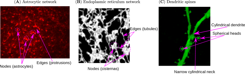
Figure 1: Biological networks illustrating composite domains. A: Network of astrocytes in the brain is made of ball (red network) connected by narrow passage (courtesy of N. Rouach): a pipette delivers here a fluorescent dyes that diffuse passively inside the network. B: Endoplasmic reticulum network, where round nodes (cisterna) are connected by narrow cylinders (courtesy of V. Kriechbaumer). C: Dendritic spines (white arrow) consist of a round head connecting a dendrite by a thin neck (courtesy of E. Korkotian).

The context associated to computing asymptotic formula for the arrival time of a Brownian particle initially located at a point $X$ inside a bounded domain $\Omega$ to a target (a narrow absorbing window $\partial\Omega_{A}$ of radius $A$) is the narrow escape theory [12, 13, 14, 15, 16, 17, 18], where most of the boundary is a reflective surface. The Mean First Passage Time (MFPT) $T(\mbox{\boldmath$X$})$, averaged over realizations is solution of the mixed boundary value problem [19]

$$\Delta T(\mbox{\boldmath$X$})=-\frac{1}{D}\,,\quad\mbox{\boldmath$X$}\in\Omega\,,$$ (1.1)

where $D$ is the diffusion coefficient of the underlying Brownian motion, with the boundary conditions

$$T(\mbox{\boldmath$X$})=0\,,\quad\mbox{\boldmath$X$}\in\partial\Omega_{A}\,,\quad\frac{\partial T(\mbox{\boldmath$X$})}{\partial\mbox{\boldmath$n$}}=0\,,\quad\mbox{\boldmath$X$}\in\partial\Omega\backslash\partial\Omega_{A}\,.$$ (1.2)

If the Dirichlet part is small enough compared to the boundary size, with $|\partial\Omega_{A}|\ll|\partial\Omega|$ and there are no smaller scale in the domain such as narrow passages [16], asymptotic analysis reveals that the leading order term of the expansion, outside a boundary layer near the absorbing window,

$$T(\mbox{\boldmath$X$})\sim\frac{|\Omega|}{4AD}\,,$$ (1.3)

and thus the MFPT does not depend on the initial position, and for multiple well-spaced exits (1.3) is divided by the total number of windows. In fact the MFPT behaves as the reciprocal of the first eigenvalue of the Laplacian with mixed Neumann-Dirichlet boundary conditions, with such singularly perturbed eigenvalue problems studied in [20, 21, 22, 23, 24].
However the formula (1.3) ceases to be valid when the window is connected to the main bulk compartment via a narrow cylindrical neck (of radius $A$ as well), and rather than $T\sim O(1/A)$ the scaling law $T\sim O(1/A^{2})$ is obtained for the MFPT [25, 26]. This yields much longer escape times, despite the fact that diffusion within narrow passages essentially happens in 1-D and could be thought as facilitated. Brownian particles can indeed diffuse in and out of the narrow passage several times, thus making the event of finding the target rare.
In this article, we study the narrow escape theory on networks made of composite domains, where large 3-D compartments alternate with narrow almost one-dimensional structures. We will formulate the mixed boundary value problem (1.1)-(1.2) on the two different domains illustrated in Fig. 2, and we shall derive asymptotic formulas for the MFPT highlighting the role played by narrow passages in controlling diffusion time scales. We shall focus on computing the diffusion time scales for such domains avoiding any singular limit as the radius of the narrow tubes tends to zero: the mixed boundary value problem (1.1)-(1.2) is instead solved assuming radial symmetry within the narrow cylindrical passages, thereby yielding 1-D solutions.

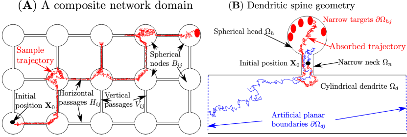
Figure 2: A: Example of a network domain of balls connected by narrow cylinders, organized in a 2-D lattice. B: Idealized geometrical representation of a dendritic spine, composed of a spherical head connected to a large cylinder via a narrow cylindrical neck. Both panels show a 2-D frontview, and starting from a position $\bm{X}$ we give a few possible Brownian trajectories.

We will consider first a general composite network domain where large spherical compartments are organized in a 2-D lattice structure, with narrow cylinders connecting each node and with a single absorbing target, as shown in Fig. 2A. For this case we will derive a sparse system of linear equations for the different MFPTs averaged over each compartment. Then we will consider a specific composite domain consisting of a spherical ball with multiple well-spaced absorbing targets, connected to a large cylindrical compartment via a narrow cylindrical passage as shown in Fig. 2B. For such a geometry inspired by the structure of the dendritic spine [9], we derive first explicit asymptotic formula for the MFPT assuming no loss from the large cylindrical bottom compartment (i.e. the opposite caps are reflecting). We then impose absorbing boundary conditions on the two flat boundaries of this large compartment, and compute the splitting probability to reach any targets located on the head boundary first, as well as the conditional MFPT.
The manuscript is organized as follows. We summarize after this paragraph the main asymptotic formulas derived in this manuscript. In Section §3, we solve the narrow escape problem on a composite network domain with 2-D lattice structure. In Section §4, we consider the dendritic spine geometry, for which explicit asymptotic formulas for the MFPT are derived. Finally, we briefly summarize our results in Section §5 in the context of cellular biology. We also mention extensions that could warrant further investigation.

2 Main asymptotic formulas derived in this manuscript

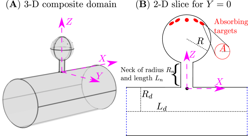
Figure 3: A: Schematic representation of a dendritic spine geometry consisting of a spherical head connecting a dendritic with a cylindrical neck. B: 2-D frontview containing the main parameters of the model.

2.1 Composite network domain

We consider a network domain consisting of $M$ by $N$ 3-D balls of radius $R$ connected by narrow cylinders of radius $R_{n}$ and length $L_{n}$, with a single narrow absorbing window of radius $A$ on the last spherical compartment. For such a rectangular lattice structure, the main result of Section §3 is a matrix equation for the vector $\bm{T}\in R^{MN}$ representing MFPTs averaged over each of the $MN$ network compartments:

$$\bm{T}=\left(\mathbb{D}_{M}\otimes I_{N}+I_{M}\otimes\mathbb{D}_{N}-\frac{4AL_{n}}{\pi R_{n}^{2}}\left(e_{M}^{M}\otimes e_{N}^{N}\right)\left(e_{M}^{M}\otimes e_{N}^{N}\right)^{T}\right)^{-1}\bm{\Xi}\,,$$ (2.1)

with $\bm{\Xi}\in\mathbb{R}^{MN}$ given by

$$\begin{split}\bm{\Xi}=&-\frac{4L_{n}R^{3}}{3R_{n}^{2}D}\left(\sum_{i=1}^{M}e_{M}^{i}\right)\otimes\left(\sum_{i=1}^{N}e_{N}^{j}\right)\\ &-\frac{L_{n}^{2}}{D}\left(\left(\frac{3}{2}\left(e_{M}^{1}+e_{M}^{M}\right)+2\sum_{i=2}^{M-1}e_{M}^{i}\right)\otimes\left(\sum_{j=1}^{N}e_{N}^{j}\right)-\frac{1}{2}\left(\sum_{i=1}^{M}e_{M}^{i}\right)\otimes\left(e_{N}^{1}+e_{N}^{N}\right)\right)\,,\end{split}$$ (2.2)

where $D$ is the diffusion coefficient. Here the vectors $e_{M}^{i}$ for $i=1,\ldots,M$ and $e_{N}^{j}$ for $j=1,\ldots,N$ form the standard orthonormal Cartesian basis in $\mathbb{R}^{M}$ and $\mathbb{R}^{N}$ respectively, while $\mathbb{D}_{M}\in\mathbb{R}^{M\times M}$ and $\mathbb{D}_{N}\in\mathbb{R}^{N\times N}$ are tridiagonal matrices corresponding to the 1-D discrete Laplacian with reflecting boundary conditions, and $\otimes$ is the Kronecker product.

2.2 Dendritic spine geometry

For a composite domain $\Omega$ consisting of a ball of radius $R$ connected to a large cylinder of radius $R_{d}$ and length $L_{d}$ via a narrow cylindrical neck of radius $R_{n}$ and length $L_{n}$, and with $n_{r}$ narrow absorbing targets of radius $A$ on the head boundary (see Fig. 3), we find in Section 4 the following asymptotic formula for the MFPT,

$$T_{n}(Z)\approx\frac{|\Omega|}{4Dn_{r}A}+\frac{L_{d}R_{d}^{2}}{DR_{n}}\left(1+\frac{L_{n}R_{n}^{2}}{L_{d}R_{d}^{2}}\right)+\frac{L_{n}L_{d}R_{d}^{2}}{DR_{n}^{2}}\left(1+\frac{L_{n}R_{n}^{2}}{2L_{d}R_{d}^{2}}\right)-\frac{ZL_{d}R_{d}^{2}}{DR_{n}^{2}}\left(1+\frac{ZR_{n}^{2}}{2L_{d}R_{d}^{2}}\right)\,,$$ (2.3)

where the starting point $Z$, with $0\leq Z\leq L_{n}$, measures the distance from the large cylindrical dendrite (Fig. 3) and $|\Omega|=\frac{4\pi R^{3}}{3}+\pi R_{n}^{2}L_{n}+\pi R_{d}^{2}L_{d}$ is the volume of the entire composite domain. Here $A$ and $R_{n}$ are two small geometrical parameters satisfying the inequality

$$\max\left\{A,R_{n}\right\}\ll\min\left\{R,R_{d},L_{n},L_{d}\right\}\,,$$ (2.4)

and we refer to equation (4.42) for a refined approximation.
When the flat boundaries of the large cylindrical dendrite (see Fig. 3) are absorbing, we derive an expression for the splitting probability of trajectories that are reaching any targets before being absorbed within the cylindrical dendrite:

$$P_{n}(Z)\approx\frac{1+\frac{Z}{R_{n}}}{2+\frac{L_{n}}{R_{n}}+\frac{\pi R_{n}}{4An_{r}}}\,,\quad\text{for }0\leq Z\leq L_{n}\,.$$ (2.5)

In that case we also obtain the approximation below for the conditional MFPT

$$\begin{split}T_{n}(Z)\approx&\frac{1}{2+\frac{L_{n}}{R_{n}}+\frac{\pi R_{n}}{4An_{r}}}\left(\frac{\pi R^{3}}{3DAn_{r}}\left(2+\frac{L_{n}}{R_{n}}+\frac{3R_{n}L_{n}^{2}}{8R^{3}}+\frac{3R_{n}^{2}L_{n}}{4R^{3}}\right)+\frac{L_{n}^{2}}{D}\left(1+\frac{L_{n}}{6R_{n}}+\frac{R_{n}}{L_{n}}\right)\right)\\ &-\frac{Z^{2}}{6D}\left(1+\frac{2}{1+\frac{Z}{R_{n}}}\right)\,,\quad\text{for }0\leq Z\leq L_{n}\,.\end{split}$$ (2.6)

3 Composite network domains

3.1 Definition of composite network domains

The composite network domain $\Omega$ made of a rectangular lattice with $M$ rows and $N$ columns is composed of 3-D balls connected by narrow cylindrical passages (Fig. 4). Each node is made of a spherical ball $B_{ij}$ of radius $R$ centered at the point $\mbox{\boldmath$X$}_{ij}$,

$$B_{ij}=\left\{\left.\mbox{\boldmath$X$}\,\right|\,\|\mbox{\boldmath$X$}-\mbox{\boldmath$X$}_{ij}\|\leq R\right\}$$ (3.1)

with $i=1,2,\ldots,M$ and $j=1,2,\ldots,N$. Horizontal narrow cylindrical neck passages $H_{ij}$ of length $L_{n}$ and radius $R_{n}$ connecting the nodes $B_{ij}$ and $B_{i(j+1)}$ are defined as

$$H_{ij}=\left\{\mbox{\boldmath$X$}=(X,Y,Z)\,\left|\,\sqrt{Y^{2}+(Z-Z_{ij})^{2}}\leq R_{n},\,X_{ij}+R\leq X\leq X_{i(j+1)}-R\right.\right\}$$ (3.2)

with $i=1,2,\ldots,M$ and $j=1,2,\ldots,N-1$, and vertical narrow cylindrical neck passages $V_{ij}$ connecting the nodes $B_{ij}$ and $B_{(i+1)j}$ are defined as

$$V_{ij}=\left\{\mbox{\boldmath$X$}=(X,Y,Z)\,\left|\,\sqrt{Y^{2}+(X-X_{ij})^{2}}\leq R_{n},\,Z_{ij}+R\leq Z\leq Z_{(i+1)j}-R\right.\right\}$$ (3.3)

with $i=1,2,\ldots,M-1$ and $j=1,2,\ldots,N$.
Using these definition, the composite domain $\Omega$ as

$$\Omega=\left(\cup_{i=1}^{M}\cup_{j=1}^{N}B_{ij}\right)\cup\left(\cup_{i=1}^{M}\cup_{j=1}^{N-1}H_{ij}\right)\cup\left(\cup_{i=1}^{M-1}\cup_{j=1}^{N}V_{ij}\right)\,.$$ (3.4)

On the boundary of the last node $\partial B_{MN}$, there is a narrow circular absorbing window $\partial\Omega_{A}$ of radius $A$ centered in $\mbox{\boldmath$X$}_{A}$, such that the full boundary of the composite domain can be decomposed as

$$\partial\Omega=\partial\Omega_{r}\cup\partial\Omega_{A},$$ (3.5)

where $\partial\Omega_{r}$ is the reflecting part and $\partial\Omega_{A}$ is absorbing. In the present manuscript, the absorbing windows are well-separated from the narrow cylindrical passages connecting to the rest of the network.

Figure 4: A rectangular lattice composite network domain. Each ball of radius $R$ is connected to its nearest neighbors via four narrow cylindrical passages. The last lattice element $B_{MN}$ contains a narrow circular absorbing window $\partial\Omega_{A}$ of radius $A$.

The dynamics inside the network is classical diffusion made of Brownian particles $W(\tau)$, with diffusion coefficient $D$ (no drift). The first escape time from the narrow absorbing target $\partial\Omega_{A}$ when starting in $\mbox{\boldmath$X$}\in\Omega$ is

$$\tau_{\mbox{\boldmath$X$}}=\min\left\{\tau\,|\,W(\tau)\in\partial\Omega_{A}\mbox{ conditioned on }W(0)=\mbox{\boldmath$X$}\right\}\,.$$ (3.6)

The Mean First Passage Time (MFPT) $T(\mbox{\boldmath$X$})$ is defined as the average over several realizations $T(\mbox{\boldmath$X$})=E(\tau_{\mbox{\boldmath$X$}})$, and it is solution of the Dynkin’s mixed boundary value problem

$$D\Delta T(\mbox{\boldmath$X$})=-1\,,\quad\mbox{ for }\mbox{\boldmath$X$}\in\Omega\,,$$ (3.7)

with boundary conditions

$$\frac{\partial T(\mbox{\boldmath$X$})}{\partial\mbox{\boldmath$n$}}=0\,,\quad\mbox{ for }\mbox{\boldmath$X$}\in\partial\Omega_{r}\,,\quad T(\mbox{\boldmath$X$})=0\,,\quad\mbox{ for }\mbox{\boldmath$X$}\in\partial\Omega_{A}\,.$$ (3.8)

In what follows, we shall derive a system of equations for the average MFPTs defined as

$$\overline{T_{ij}}=\frac{1}{|B_{ij}|}\int_{B_{ij}}T(\mbox{\boldmath$X$})d\mbox{\boldmath$X$}\,,$$ (3.9)

in the asymptotic limit of narrow cylindrical passages and absorbing window, such that

$$A\ll R,\,L_{n}\,,\quad\mbox{ and }\quad R_{n}\ll R,\,L_{n}\,.$$ (3.10)

3.2 Deriving a linear system of equations for the MFPT in a composite network

Before deriving the linear system satisfied by the average MFPT, we proceed to a non-dimensionalization of (3.7) and (3.8) by using the common radius $R$ of the ball elements, assumed to be of the same order of the length of the cylindrical passages, i. e. with $R\sim O(L_{n})$. We define the nondimensional variables

$$\mbox{\boldmath$x$}=(x,y,z)=\frac{\mbox{\boldmath$X$}}{R}\,,\quad t(\mbox{\boldmath$x$})=\frac{D}{R^{2}}T(R\mbox{\boldmath$x$})\,,\quad\mbox{ with }\mbox{\boldmath$x$}\in\omega=\frac{\Omega}{R}$$ (3.11)

with the composite domain $\omega$ defined as the following union,

$$\omega=\left(\cup_{i=1}^{M}\cup_{j=1}^{N}b_{ij}\right)\cup\left(\cup_{i=1}^{M}\cup_{j=1}^{N-1}h_{ij}\right)\cup\left(\cup_{i=1}^{M-1}\cup_{j=1}^{N}v_{ij}\right)\,,$$ (3.12)

where each $b_{ij}$ is a unit ball centered at the points $\mbox{\boldmath$x$}_{ij}=\mbox{\boldmath$X$}_{ij}/R$, while each $h_{ij}$ and $v_{ij}$ are narrow horizontal and vertical cylindrical passages of radius $r_{n}=R_{n}/R$ and length $l_{n}=L_{n}/R$. Finally the boundary $\partial\omega$ is decomposed into a reflecting part $\partial\omega_{r}$ and a narrow absorbing window $\partial\omega_{a}$ centered in $\mbox{\boldmath$x$}_{a}=\mbox{\boldmath$X$}_{a}/R$ of radius $a=A/R$. Hence we seek to solve the dimensionless mixed boundary-value problem

$$\Delta t(\mbox{\boldmath$x$})=-1\,,\quad\mbox{ for }\mbox{\boldmath$x$}\in\omega\,,$$ (3.13)

subject to

$$\frac{\partial t(\mbox{\boldmath$x$})}{\partial\mbox{\boldmath$n$}}=0\,,\quad\mbox{ for }\mbox{\boldmath$x$}\in\partial\omega_{r}\,,\quad t(\mbox{\boldmath$x$})=0\,,\quad\mbox{ for }\mbox{\boldmath$x$}\in\partial\omega_{a}\,,$$ (3.14)

by deriving a linear system of equations for the average MFPT $t_{ij}$ for each compartment,

$$\overline{t_{ij}}=\frac{1}{|b_{ij}|}\int_{b_{ij}}t(\mbox{\boldmath$x$})d\mbox{\boldmath$x$}\,,$$ (3.15)

for $i=1,\ldots,M$ and $j=1,\ldots,N$. We first proceed by reducing the dynamics through the narrow cylindrical passages to 1-D diffusion, yielding the approximation

$$t_{h_{ij}}(x)=t(\mbox{\boldmath$x$})\,,\quad\mbox{ for }\mbox{\boldmath$x$}=(x,y,z)\in h_{ij}\,,\quad t_{v_{ij}}(z)=t(\mbox{\boldmath$x$})\,,\quad\mbox{ for }\mbox{\boldmath$x$}=(x,y,z)\in v_{ij}\,.$$ (3.16)

For each subdomain $b_{ij}$, we then introduce the Neumann-Green’s function $G_{s}(\mbox{\boldmath$x$},\mbox{\boldmath$y$})$ solution of

$$\Delta G_{s}(\mbox{\boldmath$x$};\mbox{\boldmath$y$})=\frac{1}{|b_{ij}|}\,,\quad\mbox{ for }\mbox{\boldmath$x$}\in b_{ij}\,,\mbox{\boldmath$y$}\in\partial b_{ij}\,,\quad\frac{\partial}{\partial\mbox{\boldmath$n$}}G_{s}(\mbox{\boldmath$x$};\mbox{\boldmath$y$})=\delta(\mbox{\boldmath$x$}-\mbox{\boldmath$y$})\,,\quad\mbox{ for }\mbox{\boldmath$x$}\,,\mbox{\boldmath$y$}\in\partial b_{ij}\,,$$ (3.17)

and with $\int_{b_{ij}}G_{s}(\mbox{\boldmath$x$};\mbox{\boldmath$y$})d\mbox{\boldmath$x$}=0$, which expands as

$$G_{s}(\mbox{\boldmath$x$};\mbox{\boldmath$y$})=\frac{1}{2\pi\|\mbox{\boldmath$x$}-\mbox{\boldmath$y$}\|}+O\left(\log\left(\|\mbox{\boldmath$x$}-\mbox{\boldmath$y$}\|\right)\right)\,,\quad 0<\|\mbox{\boldmath$x$}-\mbox{\boldmath$y$}\|\ll 1\,,$$ (3.18)

near the singular diagonal $\mbox{\boldmath$y$}=\mbox{\boldmath$x$}$. When $i\neq N$ and $j\neq M$ we apply Green’s identity to (3.13), (3.14) and (3.17) and obtain

$$t_{h_{ij}}(x_{ij}+1)=\overline{t_{ij}}+\int_{\partial b_{ij}\cap\partial h_{ij}}G_{s}\left((\mbox{\boldmath$x$};\mbox{\boldmath$x$}_{ij}+(1,0,0)^{T}\right)\frac{\partial t(\mbox{\boldmath$x$})}{\partial\mbox{\boldmath$n$}}d\mbox{\boldmath$x$}+O(r_{n}^{2})\,,$$ (3.19)

which is readily evaluated using the integral computation from equation (A.21) of Appendix A,

$$t_{h_{ij}}(x_{ij}+1)=\overline{t_{ij}}+r_{n}\left.\frac{d}{dx}t_{h_{ij}}(x)\right|_{x=x_{ij}+1}+O(r_{n}^{2}\log(r_{n}))+O(r_{n}^{2})\,,$$ (3.20)

and finally by only keeping the average $\overline{t_{ij}}$ and dropping higher-order terms we get

$$t_{h_{ij}}(x_{ij}+1)=\overline{t_{ij}}+O(r_{n})\,.$$ (3.21)

Similarly, we obtain for the other directions,

$$t_{h_{ij}}(x_{i(j+1)}-1)=\overline{t_{i(j+1)}}+O(r_{n})\,,\quad t_{v_{ij}}(z_{ij}+1)=\overline{t_{ij}}+O(r_{n})\,,\quad t_{v_{ij}}(z_{(i+1)j}-1)=\overline{t_{(i+1)j}}+O(r_{n})\,.$$ (3.22)

In the one dimensional limit in (3.16), along with the boundary conditions given in (3.21) and (3.22) from which the $O(r_{n})$ terms were neglected, we get the boundary value problems below,

$$\frac{d^{2}t_{h_{ij}}(x)}{dx^{2}}=-1\,,\quad\mbox{ for }x_{ij}+1\leq x\leq x_{i(j+1)}-1\,,\quad t_{h_{ij}}(x_{ij}+1)=\overline{t_{ij}},\quad t_{h_{ij}}(x_{i(j+1)}-1)=\overline{t_{i(j+1)}}\,,$$ (3.23)

for $j=1,\ldots,N-1$, and

$$\frac{d^{2}t_{v_{ij}}(z)}{dz^{2}}=-1\,,\quad\mbox{ for }z_{ij}+1\leq z\leq z_{(i+1)j}-1\,,\quad t_{v_{ij}}(z_{ij}+1)=\overline{t_{ij}},\quad t_{v_{ij}}(z_{(i+1)j}-1)=\overline{t_{(i+1)j}}\,.$$ (3.24)

for $i=1,\ldots,N-1$. The solutions to (3.23) and (3.24) are

$$\begin{split}&t_{h_{ij}}(x)=\\ &-\frac{x^{2}}{2}+x\left(\frac{\overline{t_{i(j+1)}}-\overline{t_{ij}}}{l_{n}}+\frac{x_{ij}+x_{i(j+1)}}{2}\right)+\frac{\overline{t_{ij}}(x_{i(j+1)}-1)-\overline{t_{i(j+1)}}(x_{ij}+1)}{l_{n}}-\frac{(x_{ij}+1)(x_{i(j+1)}-1)}{2}\,,\end{split}$$ (3.25)

and

$$\begin{split}&t_{v_{ij}}(z)=\\ &-\frac{z^{2}}{2}+z\left(\frac{\overline{t_{(i+1)j}}-\overline{t_{ij}}}{l_{n}}+\frac{z_{ij}+z_{(i+1)j}}{2}\right)+\frac{\overline{t_{ij}}(z_{(i+1)j}-1)-\overline{t_{(i+1)j}}(z_{ij}+1)}{l_{n}}-\frac{(z_{ij}+1)(z_{(i+1)j}-1)}{2}\,.\end{split}$$ (3.26)

One condition to connect the various constant is to use the divergence theorem over each subdomain $b_{ij}$ for $i\neq 1,M$ and $j\neq 1,N$ which yields

$$\pi r_{n}^{2}\left(t_{h_{ij}}^{\prime}(x_{ij}+1)-t_{h_{i(j-1)}}^{\prime}(x_{ij}-1)+t_{v_{ij}}^{\prime}(z_{ij}+1)-t_{v_{(i-1)j}}^{\prime}(z_{ij}-1)\right)=-|b_{ij}|\,,$$ (3.27)

which becomes

$$\overline{t_{i(j+1)}}+\overline{t_{i(j-1)}}+\overline{t_{(i+1)j}}+\overline{t_{(i-1)j}}-4\overline{t_{ij}}=-\frac{|b_{ij}|l_{n}}{\pi r_{n}^{2}}-2l_{n}^{2},\quad\mbox{ for }i=2,\ldots,M-1,\,j=2,\ldots,N-1\,.$$ (3.28)

Similarly near the edges of the network we get the equations below

$$\overline{t_{i2}}+\overline{t_{(i+1)1}}+\overline{t_{(i-1)1}}-3\overline{t_{i1}} =-\frac{|b_{i1}|l_{n}}{\pi r_{n}^{2}}-\frac{3}{2}l_{n}^{2}\,,\quad i=2,\ldots,M-1,$$ (3.29)

$$\overline{t_{i(N-1)}}+\overline{t_{(i+1)N}}+\overline{t_{(i-1)N}}-3\overline{t_{iN}} =-\frac{|b_{iN}|l_{n}}{\pi r_{n}^{2}}-\frac{3}{2}l_{n}^{2}\,,\quad i=2,\ldots,M-1,$$ (3.30)

$$\overline{t_{1(j+1)}}+\overline{t_{1(j-1)}}+\overline{t_{2j}}-3\overline{t_{1j}} =-\frac{|b_{1j}|l_{n}}{\pi r_{n}^{2}}-\frac{3}{2}l_{n}^{2}\,,\quad j=2,\ldots,N-1,$$ (3.31)

$$\overline{t_{M(j+1)}}+\overline{t_{M(j-1)}}+\overline{t_{(M-1)j}}-3\overline{t_{Mj}} =-\frac{|b_{Mj}|l_{n}}{\pi r_{n}^{2}}-\frac{3}{2}l_{n}^{2}\,,\quad j=2,\ldots,N-1,$$ (3.32)

while near each corner of the network, we obtain

$$\overline{t_{21}}+\overline{t_{12}}-2\overline{t_{11}} =-\frac{|b_{11}|l_{n}}{\pi r_{n}^{2}}-l_{n}^{2}\,,$$ (3.33)

$$\frac{\pi r_{n}^{2}}{l_{n}}\left(\overline{t_{(M-1)1}}+\overline{t_{M2}}-2\overline{t_{M1}}\right) =-\frac{|b_{M1}|l_{n}}{\pi r_{n}^{2}}-l_{n}^{2}\,,$$ (3.34)

$$\overline{t_{2N}}+\overline{t_{1(N-1)}}-2\overline{t_{1N}} =-\frac{|b_{1N}|l_{n}}{\pi r_{n}^{2}}-l_{n}^{2}\,.$$ (3.35)

Finally, when $i=M$ and $j=N$, we use the classical Weber’s solution [27] to approximate the flux out of the narrow absorbing window $\partial\omega_{a}$,

$$\frac{\partial}{\partial\mbox{\boldmath$n$}}t(\mbox{\boldmath$x$})=\frac{C}{\sqrt{a^{2}-\|\mbox{\boldmath$x$}-\mbox{\boldmath$x$}_{a}\|^{2}}}\,\quad\textbf{ for }\mbox{\boldmath$x$}\in\partial\omega_{a}\,,$$ (3.36)

where $C$ is an unknown constant, that we determine using Green’s identity evaluated at the center of the exit window $\mbox{\boldmath$x$}_{a}$:

$$\begin{split}t(\mbox{\boldmath$x$}_{a})&=\overline{t_{MN}}+C\int_{\partial\omega_{a}}\frac{G_{s}(\mbox{\boldmath$x$};\mbox{\boldmath$y$})}{\sqrt{a^{2}-\|\mbox{\boldmath$x$}-\mbox{\boldmath$x$}_{a}\|^{2}}}d\mbox{\boldmath$x$}+O(r_{n}^{2})\,.\end{split}$$ (3.37)

Using the identity $t(\mbox{\boldmath$x$}_{a})=0$ as well as result (A.16) from Appendix A, we get the asymptotic relation,

$$0=\overline{t_{MN}}+C\frac{\pi}{2}+O(a\log(a))+O(r_{n}^{2})\,.$$ (3.38)

and thus

$$C=-\frac{2}{\pi}\overline{t_{MN}}+O(a\log(a))+O(r_{n}^{2})\,.$$ (3.39)

Finally, upon applying the divergence theorem over the domain $b_{MN}$ we get

$$-\pi r_{n}^{2}\left(t_{v_{(M-1)N}}^{\prime}(z_{MN}-1)+t_{h_{M(N-1)}}^{\prime}(x_{MN}-1)\right)+2\pi aC=-|b_{MN}|\,,$$ (3.40)

which becomes

$$\overline{t_{(M-1)N}}+\overline{t_{M(N-1)}}-\left(2+\frac{4al_{n}}{\pi r_{n}^{2}}\right)\overline{t_{MN}}=-\frac{|b_{MN}|l_{n}}{\pi r_{n}^{2}}-l_{n}^{2}\,,$$ (3.41)

after substituting the relation (3.39) and neglecting higher-order terms. We then define the vector $\bm{t}\in\mathbb{R}^{MN}$ of unknowns as

$$\bm{t}=\left(\overline{t_{11}},\,\ldots,\,\overline{t_{M1}},\,\overline{t_{12}},\,\ldots,\,\overline{t_{ij}},\,\overline{t_{(i+1)j}},\,\ldots,\,\overline{t_{M(N-1)}},\,\overline{t_{1N}},\,\ldots,\,\overline{t_{MN}}\right)^{T}\,,$$ (3.42)

and derive the following sparse system of linear equations,

$$\left(\mathbb{D}_{M}\otimes I_{N}+I_{M}\otimes\mathbb{D}_{N}-\frac{4al_{n}}{\pi r_{n}^{2}}\left(e_{M}^{M}\otimes e_{N}^{N}\right)\left(e_{M}^{M}\otimes e_{N}^{N}\right)^{T}\right)\bm{t}=\bm{\xi}\,.$$ (3.43)

Since $|b_{ij}|=4\pi/3$ the right-hand side $\bm{\xi}$ can be written as

$$\begin{split}\bm{\xi}=&-\frac{4l_{n}}{3r_{n}^{2}}\left(\sum_{i=1}^{M}e_{M}^{i}\right)\otimes\left(\sum_{i=1}^{N}e_{N}^{j}\right)\\ &-l_{n}^{2}\left(\left(\frac{3}{2}\left(e_{M}^{1}+e_{M}^{M}\right)+2\sum_{i=2}^{M-1}e_{M}^{i}\right)\otimes\left(\sum_{j=1}^{N}e_{N}^{j}\right)-\frac{1}{2}\left(\sum_{i=1}^{M}e_{M}^{i}\right)\otimes\left(e_{N}^{1}+e_{N}^{N}\right)\right)\,,\end{split}$$ (3.44)

where $\otimes$ is the Kronecker product, $I_{M}\in\mathbb{R}^{M\times M}$ and $I_{N}\in\mathbb{R}^{N\times N}$ are identity matrices, $e_{M}^{i}\in\mathbb{R}^{M}$ for $i=1,\,2,\,\ldots,\,M$ and $e_{N}^{j}\in\mathbb{R}^{N}$ for $j=1,\,2,\,\ldots,\,N$ are the standard cartesian basis vectors. Moreover, $\mathbb{D}_{M}$ is a $M$ by $M$ tridiagonal matrix corresponding to the discrete one-dimensional Laplacian and defined as

$$\mathbb{D}_{M}=\begin{pmatrix}-1&1&0&\cdots&0&0&0\\ 1&-2&1&\cdots&0&0&0\\ \vdots&\vdots&\vdots&\ddots&\vdots&\vdots&\vdots\\ 0&0&0&\cdots&1&-2&1\\ 0&0&0&\cdots&0&1&-1\end{pmatrix}\,\in\mathbb{R}^{M\times M}\,,$$ (3.45)

and similarly for $\mathbb{D}_{N}\in\mathbb{R}^{N\times N}$.
When the normalized radius of the absorbing window is zero $a=0$, the linear system (3.43) becomes singular: on the left-hand side we get the two-dimensional discrete Laplacian operator with reflecting boundary conditions, whose solution is defined up to a constant. Hence we have derived a discrete version of the mixed Neumann-Dirichlet elliptic PDE problem for the MFPT time on a composite network domain with a 2-D lattice structure.
Finally to account for multiple exit sites, i.e. with an absorbing target well-separated from the narrow passages on each spherical node, we simply need to replace the rank-one perturbation matrix from (3.43) by the identity matrix to obtain

$$\left(\mathbb{D}_{M}\otimes I_{N}+I_{M}\otimes\mathbb{D}_{N}-\frac{4al_{n}}{\pi r_{n}^{2}}I_{M}\otimes I_{N}\right)\bm{t}=\bm{\xi}\,.$$ (3.46)

3.3 One-dimensional lattice structure

When $M=1$, the lattice structure becomes one-dimensional (Fig. 5) and using the identities $\mathbb{D}_{1}=0$, $I_{1}=1$ and $e_{1}^{1}=1$, the linear system (3.43) simplifies to

$$\left(\mathbb{D}_{N}-\frac{4al_{n}}{\pi r_{n}^{2}}e_{N}^{N}\left(e_{N}^{N}\right)^{T}\right)\bm{t}=-\frac{4l_{n}}{3r_{n}^{2}}\left(\sum_{i=1}^{N}e_{N}^{j}\right)-l_{n}^{2}\left(\frac{1}{2}e_{N}^{1}+\sum_{j=2}^{N-1}e_{N}^{j}+\frac{1}{2}e_{N}^{N}\right)\,.$$ (3.47)

Figure 5: A composite network domain with one-dimensional lattice structure, composed of $N$ unit balls and $N-1$ narrow cylindrical passages each of length $l_{n}$.

3.4 Numerical solutions of a mixed boundary-value problem for the MFPT in a network

In this section, we compare solutions of the linear systems (3.43) and (3.47) to direct numerical simulations of the mixed boundary-value problem (3.13) and (3.14) performed with COMSOL [28]. Two different network domains are considered, one consisting of $M=3$ rows with $N=5$ columns (Fig. 6) and the other of a chain of $N=10$ ball compartments (Fig. 7). The results, given in SI units, are comparable for both cases.
The average escape times are affected by geometrical parameters of the network, as illustrated in Fig. 6B-C and Fig. 7B-C where we vary the radius and the length of the narrow passages. A good agreement is obtained between the numerical and asymptotic solutions, although a discrepancy is observed in Fig. 7C and Fig. 6C when the networks are densely packed, i.e. with the length $L_{n}$ being small. Indeed for this parameter range we have $R_{n}\sim O(L_{n})$ and the cylindrical passages are no longer narrow, explaining why the asymptotic theory ceases to be valid. Furthermore we find in Fig. 7B and Fig. 6B that the average MFPT $\overline{T_{ij}}$ decreases with the narrow passage radius $R_{n}$, with the exception of the compartment containing the narrow exit window $\partial\Omega_{A}$. Indeed, for Brownian particles starting within $B_{MN}$, bigger radius $R_{n}$ leads to longer search times since they can escape more easily through the narrow passages instead of directly reaching the absorbing target. Interestingly when the radius $R_{n}$ is large the different curves for each average MFPTs merge, indicating little influence from the location of the initial compartment.

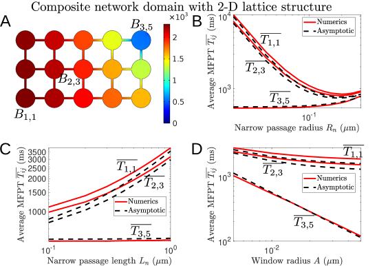
Figure 6: Composite network domain with 2-D lattice structure. A: 2-D frontview of the MFPT $T(\mbox{\boldmath$X$})$ computed numerically by solving (3.7) and (3.8) with COMSOL, for a network with $3\times 5$ compartments. Parameter values are $D=0.35\,\mu{\rm m}^{2}/{\rm ms}$, $R=0.5\,\mu{\rm m}$, $L_{n}=0.5\,\mu{\rm m}$, $R_{n}=0.05\,\mu{\rm m}$ and $A=0.01\,\mu{\rm m}$. The remaining panels show the average MFPT within the compartments $B_{1,1}$, $B_{2,3}$ and $B_{3,5}$ as a function of the radius $R_{n}$ (B) and length $L_{n}$ (C) of the narrow passages, and the target radius $A$ (D).

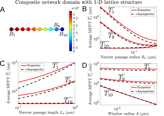
Figure 7: Composite network domain with 1-D lattice structure. A: 2-D frontview of the MFPT $T(\mbox{\boldmath$X$})$ computed numerically by solving (3.7) and (3.8) with COMSOL, for a network with $1\times 10$ compartments. Parameter values are $D=0.35\,\mu{\rm m}^{2}/{\rm ms}$, $R=0.5\,\mu{\rm m}$, $L_{n}=0.5\,\mu{\rm m}$, $R_{n}=0.05\,\mu{\rm m}$ and $A=0.01\,\mu{\rm m}$. The remaining panels show the average MFPT within the compartments $B_{1}$, $B_{9}$ and $B_{10}$ as a function of the radius $R_{n}$ (B) and length $L_{n}$ (C) of the narrow passages, and the target radius $A$ (D).

4 Time scale of diffusion between a dendrite and a dendritic spine

In this section we study a specific 3-D composite domain inspired by the structure of the dendritic spines located on neuronal cells (Figs. 2 and 3), for which we propose to derive explicit asymptotic solutions for the mean first passage times.
The domain $\Omega$ is divided into three compartments (Fig. 8),

$$\Omega=\Omega_{h}\cup\Omega_{n}\cup\Omega_{d},$$ (4.1)

where the spherical head compartment $\Omega_{h}$ has radius $R$ and is parametrized as

$$\Omega_{h}=\left\{\mbox{\boldmath$X$}=(X,Y,Z)\,\left|\,X^{2}+Y^{2}+\left(Z-L_{n}-R\right)^{2}\leq R^{2}\right.\right\}.$$ (4.2)

The cylindrical dendrite $\Omega_{d}$ has a radius $R_{d}$ and length $L_{d}$. Finally, $\Omega_{n}$ corresponding to the narrow cylindrical neck of radius $R_{n}$ and length $L_{n}$ connecting the head to the dendrite. The two cylinders are parametrized as

$$\Omega_{n} =\left\{\mbox{\boldmath$X$}=(X,Y,Z)\,\left|\,X^{2}+Y^{2}\leq R_{n}^{2}\text{ and }0\leq Z\leq L_{n}\right.\right\}\,,$$ (4.3)

$$\Omega_{d} =\left\{\mbox{\boldmath$X$}=(X,Y,Z)\,\left|\,Y^{2}+(Z+R_{d})^{2}\leq R_{d}^{2}\text{ and }-\frac{L_{d}}{2}\leq X\leq\frac{L_{d}}{2}\right.\right\}\,,$$ (4.4)

where the origin $\mbox{\boldmath$X$}=(0,0,0)$ is conveniently located at the bottom of the cylindrical neck. Since the cylindrical neck $\Omega_{n}$ acts as a narrow passage between the dendrite $\Omega_{d}$ and the spherical head $\Omega_{h}$, we imposes the conditions

$$\frac{R_{n}}{R}\ll 1\,,\quad\text{and}\quad\frac{R_{n}}{R_{d}}\ll 1.$$ (4.5)

The entrance and the exit of the narrow passage are defined as

$$\begin{split}\partial\Omega_{n}\cap\partial\Omega_{d}&=\left\{\mbox{\boldmath$X$}=(X,Y,Z)\,\left|\,Z=0\text{ and }X^{2}+Y^{2}\leq R_{n}^{2}\right.\right\}\,,\\ \partial\Omega_{n}\cap\partial\Omega_{h}&=\left\{\mbox{\boldmath$X$}=(X,Y,Z)\,\left|\,Z=L_{n}\text{ and }X^{2}+Y^{2}\leq R_{n}^{2}\right.\right\}\,,\end{split}$$ (4.6)

The boundary $\partial\Omega$ is everywhere reflective except for a collection of $n_{r}$ identical narrow targets $\partial\Omega_{hj}$ of radius $A$, located on the spherical boundary and thus defined as

$$\partial\Omega_{hj}=\left\{\mbox{\boldmath$X$}\in\partial\Omega_{h}\,|\,\|\mbox{\boldmath$X$}-\mbox{\boldmath$X$}_{j}\|\leq A\right\}\,,\quad\text{for }j=1,\ldots,n_{r}\,,\text{ with }\frac{A}{R}\ll 1.$$ (4.7)

Brownian particles can escape either from the two planar boundaries of the dendritic cylinder $\Omega_{d}$ (blue line in Fig. 8) or from circular planar absorbing disks, parametrized by

$$\partial\Omega_{dj}=\left\{\mbox{\boldmath$X$}=(X,Y,Z)\,\left|\,X=(-1)^{j}\frac{L_{d}}{2}\,,\quad Y^{2}+(Z+R_{d})^{2}\leq R_{d}^{2}\right.\right\}\,,\quad j=1,2\,.$$ (4.8)

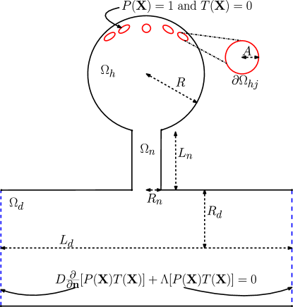
Figure 8: Schematic diagram of a spine connected to a cylindrical dendrite. The composite domain $\Omega$ consists of a spherical ball of radius $R$ on top of a narrow cylindrical passage of radius $R_{n}$ and length $L_{n}$, whose bottom end is connected to a larger cylindrical compartment of radius $R_{d}$ and length $L_{d}$.

For a starting point $X$ within the domain $\Omega$, we recall the definition of the splitting probability $P(\mbox{\boldmath$X$})$ of reaching the narrow targets $\partial\Omega_{hj}$ before escaping from the dendrite. It is defined by

$$P(\mbox{\boldmath$X$})=\text{Prob}\left\{\tau_{\mbox{\boldmath$X$}}^{A}<\tau_{\mbox{\boldmath$X$}}^{R_{d}}\right\}\,,$$ (4.9)

where $\tau_{\mbox{\boldmath$X$}}^{A}$ and $\tau_{\mbox{\boldmath$X$}}^{R_{d}}$ are random times

$$\tau_{\mbox{\boldmath$X$}}^{A} =\inf\left\{\tau\,\hbox{such that}\,W(\tau)\in\cup_{j=1}^{n_{r}}\partial\Omega_{hj}|W(0)=\mbox{\boldmath$X$}\right\}\,,$$ (4.10)

$$\tau_{\mbox{\boldmath$X$}}^{R_{d}} =\inf\left\{\tau\,\hbox{ such that }\,W(\tau)\in\cup_{j=1}^{2}\partial\Omega_{dj}|W(0)=\mbox{\boldmath$X$}\right\}\,,$$ (4.11)

where $W(\tau)$ is the underlying Brownian motion. The splitting probability $P(\mbox{\boldmath$X$})$ is solution of the Laplace’s equation [29, 30, 31]

$$D\Delta P(\mbox{\boldmath$X$})=0\,,\quad\mbox{\boldmath$X$}\in\Omega\,,$$ (4.12)

with mixed boundary conditions

$$\left\{\begin{split}&P(\mbox{\boldmath$X$})=1\,,\quad\mbox{\boldmath$X$}\in\cup_{j=1}^{n_{r}}\partial\Omega_{hj}\,,\quad\left[(-1)^{j}D\frac{\partial}{\partial X}+\Lambda\right]P(\mbox{\boldmath$X$})\to 0\,,\quad\mbox{\boldmath$X$}\in\partial\Omega_{dj}\,,\\ &D\frac{\partial}{\partial\mbox{\boldmath$n$}}P(\mbox{\boldmath$X$})\to 0\,,\quad\mbox{\boldmath$X$}\in\partial\Omega\backslash\left\{\cup_{j=1}^{n_{r}}\partial\Omega_{hj}\cup\partial\Omega_{d1}\cup\partial\Omega_{d2}\right\}\,,\end{split}\right.$$ (4.13)

where $D$ is the diffusion coefficient of the underlying Brownian motion, $\Lambda$ measures the permeability of the boundary caps $\partial\Omega_{dj}$, and $n$ is the unit normal vector to the boundary $\partial\Omega$. The Conditional Mean First Passage Time $T(\mbox{\boldmath$X$})$ is defined by

$$T(\mbox{\boldmath$X$})=E\left\{\tau_{\mbox{\boldmath$X$}}^{A}\,|\,\tau_{\mbox{\boldmath$X$}}^{A}<\tau_{\mbox{\boldmath$X$}}^{R_{d}}\,,\mbox{\boldmath$X$}(0)=\mbox{\boldmath$X$}\right\}$$ (4.14)

and satisfies [29, 30, 31]

$$D\Delta[P(\mbox{\boldmath$X$})T(\mbox{\boldmath$X$})]=-P(\mbox{\boldmath$X$})\,,\quad\mbox{\boldmath$X$}\in\Omega\,,$$ (4.15)

with boundary conditions

$$\left\{\begin{split}&P(\mbox{\boldmath$X$})T(\mbox{\boldmath$X$})=0\,,\quad\mbox{\boldmath$X$}\in\cup_{j=1}^{n_{r}}\partial\Omega_{hj}\,,\quad\left[(-1)^{j}D\frac{\partial}{\partial X}+\Lambda\right][P(\mbox{\boldmath$X$})T(\mbox{\boldmath$X$})]\to 0\,,\quad\mbox{\boldmath$X$}\in\partial\Omega_{dj}\,,\quad j=1,2\,,\\ &D\frac{\partial}{\partial\mbox{\boldmath$n$}}[P(\mbox{\boldmath$X$})T(\mbox{\boldmath$X$})]\to 0\,,\quad\mbox{\boldmath$X$}\in\partial\Omega\backslash\left\{\cup_{j=1}^{n_{r}}\partial\Omega_{hj}\cup\partial\Omega_{d1}\cup\partial\Omega_{d2}\right\}\,,\end{split}\right.$$ (4.16)

We will now either assume that the boundary of the dendritic domain is reflective, for which the permeability parameter vanishes $\Lambda=0$, or we will set $\Lambda=\infty$ thereby yielding perfectly absorbing planar boundaries of the dendritic cylinder.

4.1 Non-dimensionalization and matching conditions

We define the dimensionless variables by normalizing with the radius $R$ of the spherical domain $\Omega_{h}$, so that

$$\mbox{\boldmath$x$}=(x,y,z)=\frac{\mbox{\boldmath$X$}}{R}\,,\quad p(\mbox{\boldmath$x$})=\frac{P(R\mbox{\boldmath$x$})}{P_{0}}\,,\quad t(\mbox{\boldmath$x$})=\frac{D}{R^{2}}T(R\mbox{\boldmath$x$})\,,\quad\text{for }\mbox{\boldmath$x$}\in\omega=\frac{\Omega}{R}\,,$$ (4.17)

where $P_{0}\equiv 1$ is the characteristic splitting probability, and

$$\omega=\omega_{h}\cup\omega_{n}\cup\omega_{d}$$ (4.18)

is the rescaled composite domain with associated dimensionless geometrical parameters

$$a=\frac{A}{R}\,,\quad r_{n}=\frac{R_{n}}{R}\,,\quad l_{n}=\frac{L_{n}}{R}\,,\quad r_{d}=\frac{R_{d}}{R}\,,\quad l_{d}=\frac{L_{d}}{R}\,.$$ (4.19)

Then by defining the dimensionless membrane permeability as $\lambda=R\Lambda/D$ the mixed boundary-value problems (4.12)-(4.16) become

$$\left\{\begin{split}&\Delta p(\mbox{\boldmath$x$})=0\,,\quad\mbox{\boldmath$x$}\in\omega\,,\quad p(\mbox{\boldmath$x$})=1\,,\quad\mbox{\boldmath$x$}\in\cup_{j=1}^{n_{r}}\partial\omega_{hj}\,,\\ &\left[(-1)^{j}\frac{\partial}{\partial x}+\lambda\right]p(\mbox{\boldmath$x$})=0\,,\quad\mbox{\boldmath$x$}\in\partial\omega_{dj}\,,\quad\frac{\partial}{\partial\mbox{\boldmath$n$}}p(x)=0\,,\quad\mbox{\boldmath$x$}\in\partial\omega\backslash\left\{\cup_{j=1}^{n_{r}}\partial\omega_{hj}\cup\partial\omega_{d1}\cup\partial\omega_{d2}\right\}\,,\end{split}\right.$$ (4.20)

for the splitting probability $p(\mbox{\boldmath$x$})$. Similarly, the normalized conditional time satisfies

$$\left\{\begin{split}&\Delta[p(\mbox{\boldmath$x$})t(\mbox{\boldmath$x$})]=-p(\mbox{\boldmath$x$})\,,\quad\mbox{\boldmath$x$}\in\omega\,,\quad p(\mbox{\boldmath$x$})t(\mbox{\boldmath$x$})=0\,,\quad\mbox{\boldmath$x$}\in\cup_{j=1}^{n_{r}}\partial\omega_{hj}\,,\\ &\left[(-1)^{j}\frac{\partial}{\partial x}+\lambda\right][p(\mbox{\boldmath$x$})t(\mbox{\boldmath$x$})]=0\,,\quad\mbox{\boldmath$x$}\in\partial\omega_{dj}\,,\quad\frac{\partial}{\partial\mbox{\boldmath$n$}}[p(\mbox{\boldmath$x$})t(\mbox{\boldmath$x$})]=0\,,\quad\mbox{\boldmath$x$}\in\partial\omega\backslash\left\{\cup_{j=1}^{n_{r}}\partial\omega_{hj}\cup\partial\omega_{d1}\cup\partial\omega_{d2}\right\}\,,\end{split}\right.$$ (4.21)

for the conditional mean first passage time $t(\mbox{\boldmath$x$})$. We shall use the function

$$v(\mbox{\boldmath$x$})=t(\mbox{\boldmath$x$}){p(\mbox{\boldmath$x$})}\,,$$ (4.22)

such that the mixed boundary value problem (4.21) becomes

$$\left\{\begin{split}&\Delta v(\mbox{\boldmath$x$})=-p(\mbox{\boldmath$x$})\,,\quad\mbox{\boldmath$x$}\in\omega\,,\quad v(\mbox{\boldmath$x$})=0\,,\quad\mbox{\boldmath$x$}\in\cup_{j=1}^{n_{r}}\partial\omega_{hj}\,,\\ &\left[(-1)^{j}\frac{\partial}{\partial x}+\lambda\right]v(\mbox{\boldmath$x$})=0\,,\quad\mbox{\boldmath$x$}\in\partial\omega_{dj}\,,\quad\frac{\partial}{\partial\mbox{\boldmath$n$}}v(\mbox{\boldmath$x$})=0\,,\quad\mbox{\boldmath$x$}\in\partial\omega\backslash\left\{\cup_{j=1}^{n_{r}}\partial\omega_{hj}\cup\partial\omega_{d1}\cup\partial\omega_{d2}\right\}\,.\\ \end{split}\right.$$ (4.23)

Next we decompose (4.20) and (4.22) into three subproblems on each specific domain section $\omega_{d}$, $\omega_{n}$ and $\omega_{h}$. Within the cylindrical dendrite $\omega_{d}$, we look for a solution of

$$\Delta p_{d}(\mbox{\boldmath$x$})=0\,,\quad\Delta v_{d}(\mbox{\boldmath$x$})=-p_{d}(\mbox{\boldmath$x$})\,,\quad\text{for }\mbox{\boldmath$x$}\in\omega_{d}\,,$$ (4.24)

satisfying the boundary conditions

$$\left\{\begin{split}&\frac{\partial}{\partial\mbox{\boldmath$n$}}p_{d}(\mbox{\boldmath$x$})=0\,,\quad\frac{\partial}{\partial\mbox{\boldmath$n$}}v_{d}(\mbox{\boldmath$x$})=0\,,\quad\mbox{\boldmath$x$}\in\partial\omega_{d}\backslash\left\{\partial\omega_{n}\cup\partial\omega_{d1}\cup\omega_{d2}\right\}\,,\\ &\left[(-1)^{j}\frac{\partial}{\partial x}+\lambda\right]p_{d}(\mbox{\boldmath$x$})=0\,,\quad\left[(-1)^{j}\frac{\partial}{\partial x}+\lambda\right]v_{d}(\mbox{\boldmath$x$})=0\,,\quad\mbox{\boldmath$x$}\in\partial\omega_{dj}\,.\end{split}\right.$$ (4.25)

At the intersection boundary between the dendrite and the neck, we impose continuity matching conditions:

$$p_{n}(\mbox{\boldmath$x$})=p_{d}(\mbox{\boldmath$x$})\quad\text{and}\quad v_{n}(\mbox{\boldmath$x$})=v_{d}(\mbox{\boldmath$x$})\,,\quad x\in\partial\omega_{n}\cap\partial\omega_{d}\,,$$ (4.26)

and similarly the flux should be continuous

$$\frac{\partial}{\partial\mbox{\boldmath$n$}}p_{d}(\mbox{\boldmath$x$})=\left.\frac{\partial}{\partial z}p_{n}(\mbox{\boldmath$x$})\right|_{z=0}\quad\text{and}\quad\frac{\partial}{\partial\mbox{\boldmath$n$}}v_{d}(\mbox{\boldmath$x$})=\left.\frac{\partial}{\partial z}v_{n}(\mbox{\boldmath$x$})\right|_{z=0}\,,\quad\mbox{\boldmath$x$}\in\partial\omega_{n}\cap\partial\omega_{d}\,.$$ (4.27)

Here $p_{n}(\mbox{\boldmath$x$})$ and $v_{n}(\mbox{\boldmath$x$})$ are the splitting probability and within the neck section we have

$$\Delta p_{n}(\mbox{\boldmath$x$})=0\,,\quad\Delta v_{n}(\mbox{\boldmath$x$})=-p_{n}(\mbox{\boldmath$x$})\,,\quad\text{for }\mbox{\boldmath$x$}\in\omega_{n}\,,$$ (4.28)

along with no-flux boundary conditions on the curved cylindrical boundary,

$$\frac{\partial}{\partial\mbox{\boldmath$n$}}p_{n}(\mbox{\boldmath$x$})=0\,,\quad\frac{\partial}{\partial\mbox{\boldmath$n$}}v_{n}(\mbox{\boldmath$x$})=0\,,\quad\mbox{\boldmath$x$}\in\partial\omega_{n}\backslash\left\{\partial\omega_{d}\cup\partial\omega_{h}\right\}\,.$$ (4.29)

Additional matching conditions are imposed at the top of the neck, where it intersects with the spherical head,

$$\left\{\begin{split}p_{n}(\mbox{\boldmath$x$})&=p_{h}(\mbox{\boldmath$x$})\quad\text{and}\quad v_{n}(\mbox{\boldmath$x$})=v_{h}(\mbox{\boldmath$x$})\,,\quad x\in\partial\omega_{n}\cap\partial\omega_{h}\,,\\ \frac{\partial}{\partial\mbox{\boldmath$n$}}p_{h}(\mbox{\boldmath$x$})&=\left.-\frac{\partial}{\partial z}p_{n}(\mbox{\boldmath$x$})\right|_{z=l_{n}}\quad\text{and}\quad\frac{\partial}{\partial\mbox{\boldmath$n$}}v_{h}(\mbox{\boldmath$x$})=\left.-\frac{\partial}{\partial z}v_{n}(\mbox{\boldmath$x$})\right|_{z=l_{n}}\,,\quad\mbox{\boldmath$x$}\in\partial\omega_{n}\cap\partial\omega_{h}\,.\end{split}\right.$$ (4.30)

where $p_{h}(\mbox{\boldmath$x$})$ and $v_{h}(\mbox{\boldmath$x$})$ are the splitting probability and the function $v_{h}$ restricted to the head section $\omega_{h}$ satisfies

$$\Delta p_{h}(\mbox{\boldmath$x$})=0\,,\quad\Delta v_{h}(\mbox{\boldmath$x$})=-p_{h}(\mbox{\boldmath$x$})\,,\quad\text{for }\mbox{\boldmath$x$}\in\omega_{h}\,,$$ (4.31)

subject to mixed Neumann-Dirichlet boundary conditions

$$\left\{\begin{split}&\frac{\partial}{\partial\mbox{\boldmath$n$}}p_{h}(\mbox{\boldmath$x$})=0\,,\quad\frac{\partial}{\partial\mbox{\boldmath$n$}}v_{h}(\mbox{\boldmath$x$})=0\,,\quad\mbox{\boldmath$x$}\in\partial\omega_{h}\backslash\left\{\cup_{j=1}^{n_{r}}\partial\omega_{hj}\cup\partial\omega_{n}\right\}\,,\\ &p_{h}(\mbox{\boldmath$x$})=1\,,\quad v_{h}(\mbox{\boldmath$x$})=0\,,\quad\mbox{\boldmath$x$}\in\cup_{j=1}^{n_{r}}\partial\omega_{hj}\,.\end{split}\right.$$ (4.32)

4.2 Fully reflective dendrite boundaries

When the membrane permeability ratio $\lambda\equiv R\Lambda/D=0$ vanishes, diffusing particles cannot escape from the dendrite and thus the splitting probability is $p(\mbox{\boldmath$x$})\equiv 1$. We first define

$$\mbox{\boldmath$x$}_{d}=(0,0,0)\,,\quad\mbox{\boldmath$x$}_{h}=(0,0,l_{n})\,,$$ (4.33)

as the centers of the circular disks $\partial\omega_{n}\cap\partial\omega_{d}$ and $\partial\omega_{n}\cap\partial\omega_{h}$ connecting the narrow passage of radius $r_{n}$ between the dendrite and the spherical head. Next, the solution $v_{n}(z)$ in the thin cylindrical neck is radially symmetric and satisfies the following boundary value problem

$$\begin{split}&\frac{d^{2}}{dz^{2}}v_{n}(z)=-1\,,\quad 0\leq z\leq l_{n}\,,\quad v_{n}(0)=v_{d}(\mbox{\boldmath$x$}_{d})\,,\quad v_{n}(l_{n})=v_{h}(\mbox{\boldmath$x$}_{h})\,,\\ &\left.\frac{d}{dz}v_{n}\right|_{z=0}=\frac{\partial}{\partial\mbox{\boldmath$n$}}v_{d}(\mbox{\boldmath$x$})\,,\quad\text{for }\mbox{\boldmath$x$}\in\partial\omega_{n}\cap\partial\omega_{d}\,,\quad\left.\frac{d}{dz}v_{n}\right|_{z=l_{n}}=-\frac{\partial}{\partial\mbox{\boldmath$n$}}v_{h}(\mbox{\boldmath$x$})\,,\quad\text{for }x\in\partial\omega_{n}\cap\partial\omega_{h}\,,\end{split}$$ (4.34)

where $z$ corresponds to the distance from the dendrite. The solution is readily found to be

$$v_{n}(z)=v_{d}(\mbox{\boldmath$x$}_{d})+\left(\frac{1}{l_{n}}\left(v_{h}(\mbox{\boldmath$x$}_{h})-v_{d}(\mbox{\boldmath$x$}_{d})\right)+\frac{l_{n}}{2}\right)z-\frac{z^{2}}{2}\,.$$ (4.35)

Next, by applying the divergence theorem we show in Appendix B that the exit flux from the dendrite must satisfy

$$\frac{\partial}{\partial\mbox{\boldmath$n$}}v_{d}(\mbox{\boldmath$x$})=-\frac{|\omega_{d}|}{\pi r_{n}^{2}}\,,\quad\mbox{\boldmath$x$}\in\partial\omega_{n}\cap\omega_{d}$$ (4.36)

and thus upon using the matching condition, we get

$$\left.\frac{d}{dz}v_{n}\right|_{z=0}=\frac{1}{l_{n}}\left(v_{h}(\mbox{\boldmath$x$}_{h})-v_{d}(\mbox{\boldmath$x$}_{d})\right)+\frac{l_{n}}{2}=-\frac{|\omega_{d}|}{\pi r_{n}^{2}}.$$ (4.37)

At the intersection $\partial\omega_{n}\cap\partial\omega_{h}$, we obtain the asymptotic behavior result (Appendix A) for small $r_{n}$:

$$v_{h}(\mbox{\boldmath$x$}_{h})=\frac{1}{4an_{r}}\left(|\omega_{h}|-\pi r_{n}^{2}\left.\frac{d}{dz}v_{n}\right|_{z=l_{n}}\right)\left(1-\frac{a}{\pi}\log(a)+O(a)\right)-\left.\frac{d}{dz}v_{h}\right|_{z=l_{n}}\left(r_{n}-\frac{r_{n}^{2}}{4}\log(r_{n})+O(r_{n}^{2})\right)\,,$$ (4.38)

which becomes upon using the matching condition

$$\begin{split}v_{h}(\mbox{\boldmath$x$}_{h})&=\left(\frac{l_{n}r_{n}}{2}-\frac{r_{n}}{l_{n}}\left(v_{h}(\mbox{\boldmath$x$}_{h})-v_{d}(\mbox{\boldmath$x$}_{d})\right)\right)\left(\frac{\pi r_{n}}{4an_{r}}\left(1-\frac{a}{\pi}\log(a)+O(1)\right)+1-\frac{r_{n}}{4}\log(r_{n})+O(r_{n})\right)\\ &+\frac{|\omega_{h}|}{4an_{r}}\left(1-\frac{a}{\pi}\log(a)+O(a)\right).\end{split}$$ (4.39)

Then, upon solving (4.37) and (4.39) for $v_{d}(\mbox{\boldmath$x$}_{d})$ and $v_{h}(\mbox{\boldmath$x$}_{h})$, we obtain

$$v_{d}(\mbox{\boldmath$x$}_{d}) =\frac{|\omega|}{4an_{r}}\left(1-\frac{a}{\pi}\log(a)+O(a)\right)+l_{n}r_{n}\left(\frac{|\omega_{d}|}{|\omega_{n}|}+1\right)\left(1-\frac{r_{n}}{4}\log(r_{n})+O(r_{n})\right)+l_{n}^{2}\left(\frac{1}{2}+\frac{|\omega_{d}|}{|\omega_{n}|}\right)\,,$$

$$v_{h}(\mbox{\boldmath$x$}_{h}) =\frac{|\omega|}{4an_{r}}\left(1-\frac{a}{\pi}\log(a)+O(a)\right)+l_{n}r_{n}\left(\frac{|\omega_{d}|}{|\omega_{n}|}+1\right)\left(1-\frac{r_{n}}{4}\log(r_{n})+O(r_{n})\right)\,,$$

where $|\omega|$ is the volume of the composite domain

$$|\omega|=|\omega_{h}|+|\omega_{n}|+|\omega_{d}|=\frac{4\pi}{3}+\pi r_{n}^{2}l_{n}+\pi r_{d}^{2}l_{d}\,,$$ (4.40)

and thus within the neck $v_{n}(z)$, we have

$$\begin{split}v_{n}(z)&=\frac{|\omega|}{4an_{r}}\left(1-\frac{a}{\pi}\log(a)+O(a)\right)+l_{n}r_{n}\left(\frac{|\omega_{d}|}{|\omega_{n}|}+1\right)\left(1-\frac{r_{n}}{4}\log(r_{n})+O(r_{n})\right)\\ &+l_{n}^{2}\left(\frac{1}{2}+\frac{|\omega_{d}|}{|\omega_{n}|}\right)-z^{2}\left(\frac{|\omega_{d}|}{|\omega_{n}|}\frac{l_{n}}{z}+\frac{1}{2}\right)\,.\end{split}$$ (4.41)

Since the splitting probability satisfies $p_{n}(z)=1$ we simply need to multiply (4.41) by the factor $R^{2}/D$ to obtain the formula for the MFPT $T_{n}(Z)$ with all the dimensional parameters,

$$\begin{split}T_{n}(Z)&=\frac{|\Omega|}{4Dn_{r}A}\left(1-\frac{A}{\pi R}\log\left(\frac{A}{R}\right)+O\left(\frac{A}{R}\right)\right)+\frac{L_{d}R_{d}^{2}}{DR_{n}}\left(1+\frac{L_{n}R_{n}^{2}}{L_{d}R_{d}^{2}}\right)\left(1-\frac{R_{n}}{4R}\log\left(\frac{R_{n}}{R}\right)+O\left(\frac{R_{n}}{R}\right)\right)\\ &+\frac{L_{n}L_{d}R_{d}^{2}}{DR_{n}^{2}}\left(1+\frac{L_{n}R_{n}^{2}}{2L_{d}R_{d}^{2}}\right)-\frac{ZL_{d}R_{d}^{2}}{DR_{n}^{2}}\left(1+\frac{ZR_{n}^{2}}{2L_{d}R_{d}^{2}}\right)\,,\quad\text{for }0\leq Z\leq L_{n}\,,\end{split}$$ (4.42)

where $|\Omega|=\frac{4\pi R^{3}}{3}+\pi R_{n}^{2}L_{n}+\pi R_{d}^{2}L_{d}$ is the volume of the entire composite domain.

4.3 Computing the splitting probability when particles in the dendrite can be lost

We now analyze the case where Brownian particles are absorbed by the circular planar boundaries of the dendrite, which is obtained by taking the surface permeability to be $\lambda=\infty$. We study the fraction of these particles that reaches a narrow target (the splitting probability). Given that they have reached the targets, we compute the conditional mean first passage time.
We first seek an asymptotic approximation for the splitting probability $p(\mbox{\boldmath$x$})$. In the thin cylindrical neck $\Omega_{n}$, the splitting probability $p_{n}(z)$ satisfies the boundary value problem

$$\left\{\begin{split}&\frac{d^{2}}{dz^{2}}p_{n}(z)=0\,,\quad 0\leq z\leq l_{n}\,,\quad p_{n}(0)=p_{d}(\mbox{\boldmath$x$}_{d})\,,\quad p_{n}(l_{n})=p_{h}(\mbox{\boldmath$x$}_{h})\,,\\ &\left.\frac{d}{dz}p_{n}\right|_{z=0}=\frac{\partial}{\partial\mbox{\boldmath$n$}}p_{d}(\mbox{\boldmath$x$})\,,\quad\mbox{\boldmath$x$}\in\partial\omega_{n}\cap\partial\omega_{d}\quad\left.\frac{d}{dz}p_{n}\right|_{z=l_{n}}=-\frac{\partial}{\partial\mbox{\boldmath$n$}}p_{h}(\mbox{\boldmath$x$})\,,\quad\mbox{\boldmath$x$}\in\partial\omega_{n}\cap\partial\omega_{h}\,,\end{split}\right.$$ (4.43)

which readily solves as

$$p_{n}(z)=\left(p_{h}(\mbox{\boldmath$x$}_{h})-p_{d}(\mbox{\boldmath$x$}_{d})\right)\frac{z}{l_{n}}+p_{d}(\mbox{\boldmath$x$}_{d})\,,\quad 0\leq z\leq l_{n}\,.$$ (4.44)

Here $p_{d}(\mbox{\boldmath$x$}_{d})$ and $p_{h}(\mbox{\boldmath$x$}_{h})$ are the splitting probabilities at the bottom and top sections of the neck, whose expressions are obtained by an asymptotic expansion (Appendix A and B). The results are

$$p_{d}(\mbox{\boldmath$x$}_{d})=\left.\frac{d}{dz}p_{n}\right|_{z=0}r_{n}=\left(p_{h}(\mbox{\boldmath$x$}_{h})-p_{d}(\mbox{\boldmath$x$}_{d})\right)\frac{r_{n}}{l_{n}}\,,$$ (4.45)

and

$$p_{h}(\mbox{\boldmath$x$}_{h})=1-\left.\frac{d}{dz}p_{n}\right|_{z=l_{n}}\left(\frac{\pi r_{n}^{2}}{4an_{r}}+r_{n}\right)=1-\frac{r_{n}}{l_{n}}\left(p_{h}(\mbox{\boldmath$x$}_{h})-p_{d}(\mbox{\boldmath$x$}_{d})\right)\left(\frac{\pi r_{n}}{4an_{r}}+1\right)\,,$$ (4.46)

where we only kept the leading order terms in $a\ll 1$ and $r_{n}\ll 1$. Upon solving equations (4.45) and (4.46) we find

$$p_{d}(\mbox{\boldmath$x$}_{d})=\frac{1}{\mu}\,,\quad p_{h}(\mbox{\boldmath$x$}_{h})=\frac{1+\frac{l_{n}}{r_{n}}}{\mu}\,,\quad\text{with}\quad\mu=2+\frac{l_{n}}{r_{n}}+\frac{\pi r_{n}}{4an_{r}}\,.$$ (4.47)

and thus we get within the neck

$$p_{n}(z)=\frac{1+\frac{z}{r_{n}}}{\mu}\,,\quad 0\leq z\leq l_{n}\,.$$ (4.48)

The probability of reaching a single specific target $\partial\omega_{hj}$ is recovered after dividing by the total number $n_{r}$. Finally, the dimensional formula associated to (4.48) is given by

$$P_{n}(Z)=\frac{1+\frac{Z}{R_{n}}}{2+\frac{L_{n}}{R_{n}}+\frac{\pi R_{n}}{4An_{r}}}+O\left(\left(\frac{R_{n}}{R}\right)^{2}\log\left(\frac{A}{R}\right)\right)\,,\quad\text{for }0\leq Z\leq L_{n}\,.$$ (4.49)

4.4 Conditional MFPTs for particles absorbed by the dendrite

We now solve for the conditional mean first passage time in the thin cylindrical neck limit: the function $v_{n}(z)$ satisfies the boundary value problem

$$\left\{\begin{split}&\frac{d^{2}}{dz^{2}}v_{n}(z)=-p_{n}(z)=-\frac{1+\frac{z}{r_{n}}}{\mu}\,,\quad 0\leq z\leq l_{n}\,,\quad v_{n}(0)=v_{d}(\mbox{\boldmath$x$}_{d})\,,\quad v_{n}(l_{n})=v_{h}(\mbox{\boldmath$x$}_{h})\,,\\ &\left.\frac{d}{dz}v_{n}\right|_{z=0}=\frac{\partial}{\partial\mbox{\boldmath$n$}}v_{d}(\mbox{\boldmath$x$})\,,\quad\mbox{\boldmath$x$}\in\partial\omega_{n}\cap\partial\omega_{d}\,,\quad\left.\frac{d}{dz}v_{n}\right|_{z=l_{n}}=-\frac{\partial}{\partial\mbox{\boldmath$n$}}v_{h}(\mbox{\boldmath$x$})\,,\quad\mbox{\boldmath$x$}\in\partial\omega_{n}\cap\partial\omega_{h}\,,\end{split}\right.$$ (4.50)

where $v_{d}(\mbox{\boldmath$x$}_{d})$ and $v_{h}(\mbox{\boldmath$x$}_{h})$ are solutions within the dendrite and head compartments respectively. After integrating with respect to the distance $Z$ from the dendrite, we get

$$v_{n}(z)=v_{d}(\mbox{\boldmath$x$}_{d})+\left(\frac{1}{l_{n}}\left(v_{h}(\mbox{\boldmath$x$}_{h})-v_{d}(\mbox{\boldmath$x$}_{d})\right)+\frac{\frac{l_{n}}{2}+\frac{l_{n}^{2}}{6r_{n}}}{\mu}\right)z-\left(\frac{\frac{z^{2}}{2}+\frac{z^{3}}{6r_{n}}}{\mu}\right)\,,\quad 0\leq z\leq l_{n}.$$ (4.51)

Keeping the leading order terms in $a$ and $r_{n}$ from equations (A.33) and (B.28), we get

$$v_{d}(\mbox{\boldmath$x$}_{d})=\left.\frac{d}{dz}v_{n}\right|_{z=0}r_{n}=\left(v_{h}(\mbox{\boldmath$x$}_{h})-v_{d}(\mbox{\boldmath$x$}_{d})\right)\frac{r_{n}}{l_{n}}+\frac{\frac{l_{n}r_{n}}{2}+\frac{l_{n}^{2}}{6}}{\mu}$$ (4.52)

as well as

$$v_{h}(\mbox{\boldmath$x$}_{h}) =\frac{1}{4an_{r}}\left(|\omega_{h}|\overline{p_{h}}-\left.\frac{d}{dz}v_{n}\right|_{z=l_{n}}\pi r_{n}^{2}\right)-\left.\frac{d}{dz}v_{n}\right|_{z=l_{n}}r_{n}$$

$$=\frac{|\omega_{h}|\overline{p_{h}}}{4an_{r}}+\left(\frac{\frac{l_{n}r_{n}}{2}+\frac{l_{n}^{2}}{3}}{\mu}-\frac{r_{n}}{l_{n}}\left(v_{h}(\mbox{\boldmath$x$}_{h})-v_{d}(\mbox{\boldmath$x$}_{d})\right)\right)\left(\frac{\pi r_{n}}{4an_{r}}+1\right)\,.$$ (4.53)

Here $\overline{p_{h}}$ is the average splitting probability over the head domain $\omega_{h}$, whose leading order approximation is

$$\overline{p_{h}}=1-\frac{\pi r_{n}^{2}}{4an_{r}}\left.\frac{d}{dz}p_{n}\right|_{z=l_{n}}=1-\frac{\pi r_{n}}{4an_{r}\mu}=\frac{2+\frac{l_{n}}{r_{n}}}{\mu}\,,$$ (4.54)

as obtained from formula (A.19) of Appendix A. Then, upon solving (4.52) and (4.4) for $v_{d}(\mbox{\boldmath$x$}_{d})$ and $v_{h}(\mbox{\boldmath$x$}_{h})$, we obtain

$$v_{d}(\mbox{\boldmath$x$}_{d})=\frac{1}{\mu}\left(\frac{|\omega_{h}|}{4an_{r}}\left(\frac{2+\frac{l_{n}}{r_{n}}}{\mu}+\frac{\pi r_{n}l_{n}^{2}}{2|\omega_{h}|\mu}+\frac{\pi r_{n}^{2}l_{n}}{|\omega_{h}|\mu}\right)+\frac{l_{n}^{3}}{6r_{n}\mu}+\frac{l_{n}^{2}}{\mu}+\frac{r_{n}l_{n}}{\mu}\right)\,,$$ (4.55)

as well as

$$v_{h}(\mbox{\boldmath$x$}_{h})=\frac{1+\frac{l_{n}}{r_{n}}}{\mu}\left(\frac{|\omega_{h}|}{4an_{r}}\left(\frac{2+\frac{l_{n}}{r_{n}}}{\mu}+\frac{\pi r_{n}l_{n}^{2}}{2|\omega_{h}|\mu}+\frac{\pi r_{n}^{2}l_{n}}{|\omega_{h}|\mu}\right)+\frac{l_{n}^{3}}{6r_{n}\mu}+\frac{l_{n}^{2}}{\mu}+\frac{r_{n}l_{n}}{\mu}\right)-\frac{\frac{l_{n}^{2}}{2}+\frac{l_{n}^{3}}{6r_{n}}}{\mu}\,.$$ (4.56)

For $0\leq z\leq l_{n}$, this therefore yields

$$v_{n}(z)=\frac{1+\frac{z}{r_{n}}}{\mu}\left(\frac{|\omega_{h}|}{4an_{r}}\left(\frac{2+\frac{l_{n}}{r_{n}}}{\mu}+\frac{3r_{n}l_{n}^{2}}{8\mu}+\frac{3r_{n}^{2}l_{n}}{4\mu}\right)+\frac{l_{n}^{3}}{6r_{n}\mu}+\frac{l_{n}^{2}}{\mu}+\frac{r_{n}l_{n}}{\mu}\right)-\left(\frac{\frac{z^{2}}{2}+\frac{z^{3}}{6r_{n}}}{\mu}\right)\,,$$ (4.57)

where the volume of the head is $|\omega_{h}|=4\pi/3$. To recover the conditional mean first passage times for an arbitrary starting point within the neck, we divide by the splitting probability to obtain

$$t_{n}(z)=\frac{v_{n}(z)}{p_{n}(z)}=\left(\frac{|\omega_{h}|}{4an_{r}}\left(\frac{2+\frac{l_{n}}{r_{n}}}{\mu}+\frac{3r_{n}l_{n}^{2}}{8\mu}+\frac{3r_{n}^{2}l_{n}}{4\mu}\right)+\frac{l_{n}^{3}}{6r_{n}\mu}+\frac{l_{n}^{2}}{\mu}+\frac{r_{n}l_{n}}{\mu}\right)-\frac{z^{2}}{6}\left(1+\frac{2}{1+\frac{z}{r_{n}}}\right)\,,$$ (4.58)

which reduces to

$$t_{n}(z)=\frac{1}{2+\frac{l_{n}}{r_{n}}+\frac{\pi r_{n}}{4an_{r}}}\left(\frac{|\omega_{h}|}{4an_{r}}\left(2+\frac{l_{n}}{r_{n}}+\frac{3r_{n}l_{n}^{2}}{8}+\frac{3r_{n}^{2}l_{n}}{4}\right)+\frac{l_{n}^{3}}{6r_{n}}+l_{n}^{2}+r_{n}l_{n}\right)-\frac{z^{2}}{6}\left(1+\frac{2}{1+\frac{z}{r_{n}}}\right)\,.$$ (4.59)

This yields for a particle starting at the intersection of the neck with the dendrite

$$t_{d}(\mbox{\boldmath$x$}_{d})=\frac{1}{2+\frac{l_{n}}{r_{n}}+\frac{\pi r_{n}}{4an_{r}}}\left(\frac{|\omega_{h}|}{4an_{r}}\left(2+\frac{l_{n}}{r_{n}}+\frac{3r_{n}l_{n}^{2}}{8}+\frac{3r_{n}^{2}l_{n}}{4}\right)+\frac{l_{n}^{3}}{6r_{n}}+l_{n}^{2}+r_{n}l_{n}\right)\,,$$ (4.60)

and for those starting at the upper neck cross section, we have

$$t_{h}(\mbox{\boldmath$x$}_{h})=\frac{1}{2+\frac{l_{n}}{r_{n}}+\frac{\pi r_{n}}{4an_{r}}}\left(\frac{|\omega_{h}|}{4an_{r}}\left(2+\frac{l_{n}}{r_{n}}+\frac{3r_{n}l_{n}^{2}}{8}+\frac{3r_{n}^{2}l_{n}}{4}\right)+\frac{l_{n}^{3}}{6r_{n}}+l_{n}^{2}+r_{n}l_{n}\right)-\frac{l_{n}^{2}}{6}\left(1+\frac{2}{1+\frac{l_{n}}{r_{n}}}\right)\,.$$ (4.61)

Finally we set $T_{n}(Z)=R^{2}/Dt_{n}(Z/R)$ and obtain the conditional MFPT formula equivalent to (4.59) with dimensional units:

$$\begin{split}T_{n}(Z)&=\frac{1}{2+\frac{L_{n}}{R_{n}}+\frac{\pi R_{n}}{4An_{r}}}\left(\frac{\pi R^{3}}{3DAn_{r}}\left(2+\frac{L_{n}}{R_{n}}+\frac{3R_{n}L_{n}^{2}}{8R^{3}}+\frac{3R_{n}^{2}L_{n}}{4R^{3}}\right)+\frac{L_{n}^{2}}{D}\left(1+\frac{L_{n}}{6R_{n}}+\frac{R_{n}}{L_{n}}\right)\right)\\ &-\frac{Z^{2}}{6D}\left(1+\frac{2}{1+\frac{Z}{R_{n}}}\right)+O\left(\log\left(\frac{A}{R}\right)\right)\,,\quad\text{for }0\leq Z\leq L_{n}\,.\end{split}$$ (4.62)

4.5 Asymptotic formulas versus numerical simulations

We now compare the asymptotic formulas for the splitting probability and the conditional MFPT against numerical solutions of the mixed boundary value problems (4.20) and (4.21) performed with COMSOL [28]. Additional stochastic simulations are also performed, but only for the case where Brownian particles are absorbed upon hitting the lateral boundaries of the cylindrical dendrite. All results are shown with dimensional units and the parameter values are summarized in Table 1.
We first consider in Fig. 9 the case where no particles are lost from the dendrite, i.e. $\Lambda=0$ and the splitting probability is $P(\mbox{\boldmath$X$})=1$. Then we set $\Lambda=\infty$ and analyze how the narrow exits radius, as well as the length and the radius of the cylindrical neck, affect the splitting probability and the conditional MFPT (Fig. 10-12). Finally for all the numerical experiments either $n_{r}=1,\,5$ or $50$ targets are added to the spherical boundary $\partial\Omega_{h}$.

Table 1: List of parameter values

Parameter	Symbol	Value	Non-dim. parameter	Non-dim. value
Spine head radius	$R$	0.5 $\mu$m	$R/R$	$1$
Spine neck radius	$R_{n}$	0.15 $\mu$m	$r_{n}=R_{n}/R$	$0.3$
Spine neck length	$L_{n}$	0.5 $\mu$m	$l_{n}=L_{n}/R$	$1$
Dendrite radius	$R_{d}$	1 $\mu$m	$r_{d}=R_{d}/R$	$2$
Dendrite length	$L_{d}$	5 $\mu$m	$l_{d}=L_{d}/R$	$10$
Circular target radius	$A$	0.01 $\mu$m	$a=A/R$	$0.02$
Number of targets	$n_{r}$	$50$	$-$	$-$
Diffusion coefficient	$D$	350 $\mu{\rm m}^{2}{\rm s}^{-1}$	$-$	$-$

4.6 Case $\Lambda=0$

When $\Lambda=0$ the splitting probability is $P(\mbox{\boldmath$X$})=1$ and Brownian particles can only escape from the dendrite through the narrow cylindrical neck. We show that adding more targets on the head boundary $\partial\Omega_{h}$ reduces the average search times by an equivalent factor: when they are well-spaced, twice as many targets halve the MFPT. Also the average search time decreases linearly as the starting point $Z$ approaches the spherical head (Fig. 9A). We then set the initial position at $Z=L_{n}$ and perform a sweep of the different parameters characterizing the geometry of the dendritic spine (Fig. 9B-F). Our asymptotic analysis predicts that increasing the volume of the dendrite yields longer average escape times (Fig. 9B-C). We recover the usual $1/A$ reciprocity relation [15] as the targets radius $A$ increases, as shown in Fig. 9D.
Finally, we report in Fig. 9E-F that the MFPT $T_{n}(L_{n})$ is not significantly affected by neck length variations, while we obtain the $1/R_{n}^{2}$ dependency as the radius of the narrow passage is increased, a relation also obtained for calcium ions that are reaching the bottom of the neck [25, 26]. In each plot, we find a good agreement between the asymptotic solution (dashed curve) and the numerical solution (full curve).

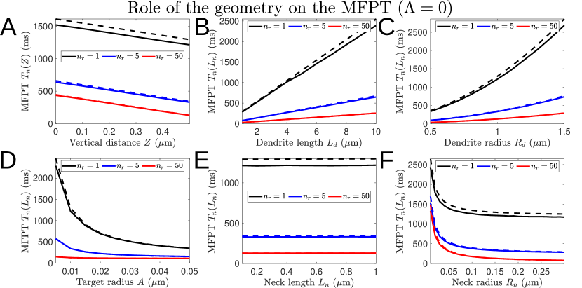
Figure 9: Effects of the geometry on the MFPT, case $\Lambda=0$. (A): MFPT $T_{n}(Z)$ as a function of the distance $Z$ from the dendrite. (B)-(C): We set $Z=L_{n}$ and vary the length $L_{d}$ and the radius $R_{d}$ of the cylindrical dendrite. (D): The MFPT $T_{n}(L_{n})$ is instead shown as a function of the target radius $A$. (E)-(F): Parameter sweeps of the narrow cylindrical neck of length $L_{n}$ and radius $R_{n}$ are performed. The dashed and full curves correspond to the asymptotic and COMSOL numerical solutions.

4.7 Case $\Lambda=\infty$

We now turn to the case where Brownian particles are absorbed upon hitting the lateral boundaries of the cylindrical dendrite $\partial\Omega_{d1}$ and $\partial\Omega_{d2}$. First, because we conditioned on the particles reaching any targets on the boundary of the head, the MFPT decays drastically from a few hundreds to a few tens of milliseconds when comparing both $\Lambda=0$ and $\Lambda=\infty$ cases. We find that the splitting probability increases linearly with the distance $Z$ from the dendrite, as shown in Fig. 10B. However this is little variations of the conditional MFPT (Fig. 10C).
The splitting probability increases with the target radius $A$, while the conditional MFPT behaves as $O(1/A)$ as expected from the asymptotic formula (4.61) (Fig. 10E)-F).
Finally, we analyze how the geometry of the narrow cylindrical neck affects the splitting probability and the conditional MFPT (Fig. 11). Upon setting $Z=L_{n}$ as the initial position, we find that the splitting probability increases with the neck length $L_{n}$, while it decreases with the neck radius $R_{n}$. Similar behaviors are obtained for the conditional MFPT $T_{n}(L_{n})$ in Fig. 11C and F, although we remark that for large number of targets varying the neck dimensions does not influence the mean binding times significantly.
Interestingly modifying the starting point from the top to the base of the neck only provides qualitatively different behavior for the splitting probability, as shown in Fig. 12, where we remark that increasing the length of the neck yields a smaller probability of reaching any targets. For small target numbers, we obtain that the splitting probability $P_{n}(0)$ behaves non-monotonically as the radius of the neck increases (Fig. 12E): there is an intermediate $R_{n}$ value on the range $[0.01,\,0.3]\,\mu{\rm m}$ for which the splitting probability is maximized. For a large number of targets this maximum is achieved for physiologically non-realistic neck radius values.
Finally, we remark that the stochastic simulation results agree qualitatively with the asymptotic solutions (Fig. 10 and 11) as well as the numerical solutions of the mixed boundary-value problem obtained with COMSOL. The discrepancy observed tends to shrink for larger target numbers, and also as the target and neck radii increase.

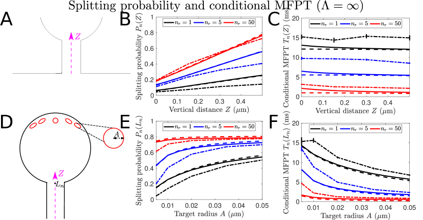
Figure 10: The top panels give the splitting probability $P_{n}(Z)$ (B) and the conditional MFPT $T_{n}(Z)$ (C) within the narrow cylindrical neck, as a function of the distance $Z$ from the dendrite. In panels (D)-(F), we set $Z=L_{n}$ and show the same quantity as a function of the narrow target radius $A$. In each panel we show the asymptotic solution (dashed-curved), the COMSOL numerical solution (full curve) and the stochastic simulation results (dot-dashed curve, with the vertical bars indicating the standard deviation) for three target numbers: $n_{r}=1$ (black), $n_{r}=5$ (blue) and $n_{r}=50$ (red).

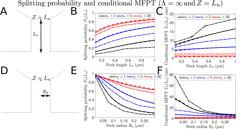
Figure 11: In the top panels we set $Z=L_{n}$ and give the splitting probability $P_{n}(L_{n})$ (B) and the conditional MFPT $T_{n}(L_{n})$ (C) as a function of the neck length $L_{n}$. In panels (D)-(F) we show the same quantity as a function of the neck radius $R_{n}$. In each panel we show the asymptotic solution (dashed-curved), the COMSOL numerical solution (full curve) and the stochastic simulation results (dot-dashed curve, with the vertical bars indicating the standard deviation) for three target numbers: $n_{r}=1$ (black), $n_{r}=5$ (blue) and $n_{r}=50$ (red).

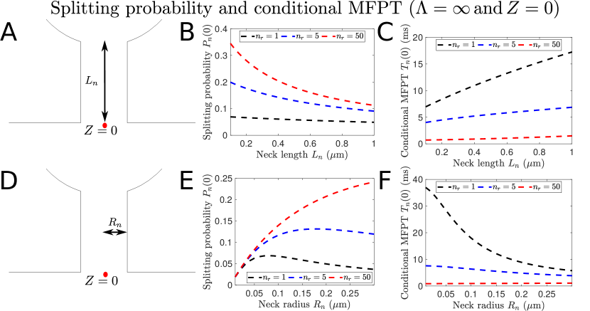
Figure 12: In the top panels we set $Z=0$ and give the splitting probability $P_{n}(0)$ (B) and the conditional MFPT $T_{n}(0)$ (C) as a function of the neck length $L_{n}$. In panels (D)-(F) we show the same quantity as a function of the neck radius $R_{n}$. In each panel we only show the asymptotic solution (dashed-curved) for three target numbers: $n_{r}=1$ (black), $n_{r}=5$ (blue) and $n_{r}=50$ (red).

5 Discussion and concluding remarks

In this manuscript, we modeled diffusion in heterogeneous network with large spherical nodes and thin cylindrical tubules. We derived asymptotic formulas for the mean time a Brownian particle takes to escape from various 3-D composite domains, i.e. with both large and short scales, with reflecting boundaries everywhere except for a collection of narrow absorbing windows. We formulated the mixed Neumann-Dirichlet boundary value problem for the Mean First Passage Time (MFPT) $T(\mbox{\boldmath$X$})$ on a composite network domain with $M$ by $N$ identical ball compartments connected by narrow cylinders (section §3).
Using asymptotic analysis we derived a sparse linear system of equations for the MFPT averaged over each compartment, that can be solved numerically. In the absence of absorbing targets, the linear system is singular and consists of a tridiagonal matrix analogous to the 2-D discrete Laplacian with reflecting boundary conditions. For a single target, there is an additional rank-one perturbation matrix that is linearly proportional to the target radius and narrow passage length, and which scales as the reciprocal of the square of the radius of the narrow passage. Then we considered a composite domain consisting of a sphere with multiple well-spaced absorbing targets (section §4 ), that is connected to a large cylindrical compartment by a narrow cylindrical neck (Fig. 13A). For Brownian particles starting at the bottom of the neck, we obtain the formula

$$\begin{split}T_{n}(0)=&\frac{\left(\frac{\pi R^{3}}{3}+\frac{\pi R_{n}^{2}L_{n}}{4}+\frac{\pi R_{d}^{2}L_{d}}{4}\right)}{Dn_{r}A}\left(1-\frac{A}{\pi R}\log\left(\frac{A}{R}\right)\right)+\frac{L_{d}R_{d}^{2}}{DR_{n}}\left(1+\frac{L_{n}R_{n}^{2}}{L_{d}R_{d}^{2}}\right)\left(1-\frac{R_{n}}{4R}\log\left(\frac{R_{n}}{R}\right)\right)\\ &+\frac{L_{n}L_{d}R_{d}^{2}}{DR_{n}^{2}}\left(1+\frac{L_{n}R_{n}^{2}}{2L_{d}R_{d}^{2}}\right).\end{split}$$ (5.1)

Thus the MFPT scales with the total volume of the composite domain, as the reciprocal of the targets size, and also as the reciprocal of the square of the radius of the narrow passage. Using parameter values gathered in Table 1, we obtain a numerical value $T_{n}(0)\approx 450\,{\rm ms}$ for the diffusion timescale from the dendrite to a small target located in the spine head.
When the larger cylindrical compartment (dendrite) is neglected (Fig. 13B), or simply no passage is possible (imposed by a mitochondria in the context of a neuron), which is equivalent to imposing reflecting boundary conditions at the bottom section of the narrow neck, then the formula (5.1) reduces to

$$T_{n}(0)=\frac{\left(\frac{\pi R^{3}}{3}+\frac{\pi R_{n}^{2}L_{n}}{4}\right)}{Dn_{r}A}\left(1-\frac{A}{\pi R}\log\left(\frac{A}{R}\right)\right)+\frac{L_{n}R_{n}}{D}\left(1-\frac{R_{n}}{4R}\log\left(\frac{R_{n}}{R}\right)\right)+\frac{L_{n}^{2}}{2D}\,,$$ (5.2)

which leads to the numerical approximation $T_{n}(0)\approx 1.41\,{\rm ms}$, which is nearly 300 times faster than for the full geometry case. Interestingly there is no singular term in $1/R_{n}^{2}$ compared to equation 5.1.
In case of partial absorption due to the presence of an organelle, we thus expect a time that can be modulated between few to hundreds of milliseconds. This time scale is relevant for quantifying the diffusion of ATP molecules generated by mitochondria and that needs to translocate into dendritic spine to maintain energy integrity.
We also analyzed the case where Brownian particles can be absorbed upon hitting the two opposite flat boundaries of the large cylindrical compartment. We derived a formula for the splitting probability of reaching the head and binding to the absorbing targets,

$$P_{n}(0)=\frac{1}{2+\frac{L_{n}}{R_{n}}+\frac{\pi R_{n}}{4An_{r}}}\approx 0.18\,,$$ (5.3)

and also the corresponding conditional MFPT,

$$T_{n}(0)=\frac{1}{2+\frac{L_{n}}{R_{n}}+\frac{\pi R_{n}}{4An_{r}}}\left(\frac{\pi R^{3}}{3DAn_{r}}\left(2+\frac{L_{n}}{R_{n}}+\frac{3R_{n}L_{n}^{2}}{8R^{3}}+\frac{3R_{n}^{2}L_{n}}{4R^{3}}\right)+\frac{L_{n}^{2}}{D}\left(1+\frac{L_{n}}{6R_{n}}+\frac{R_{n}}{L_{n}}\right)\right)\approx 0.98\,{\rm ms}\,.$$ (5.4)

for particles starting at the base of the neck $(Z=0)$. Hence, nearly one out of five particles will reach the head and bind to the targets, for an average diffusion time of one millisecond, of the same order of magnitude as predicted by the formula (5.2).

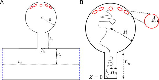
Figure 13: Schematic diagram of the dendritic spine. A: Full geometry with the ball of radius $R$ with the two cylindrical compartments. B: Simplified geometry where the large bottom cylindrical compartment is neglected. The Brownian path in black indicates a successful trajectory reaching a target starting from the neck base.

Finally, it would be valuable to derive higher-order asymptotic formulas revealing the role of the organization of the absorbing windows on the MFPT. Such expansions were developed for the unit ball [15] using strong localized perturbation theory. Another possible extension would be to develop a narrow escape theory for more general composite network domains than the ones considered in Section §3, with different number of connections per each node, narrow passages of various lengths that could not necessarily be oriented perpendicularly to each node, and also with multiple exit sites, potentially located on several spherical compartments.

Appendix A Appendix: Mixed boundary-value problems in the unit ball

In this appendix we restrict our analysis of the composite domain to the spherical section $\omega_{h}$, defined as the unit ball $\omega_{h}=\{\mbox{\boldmath$x$}\in\mathbb{R}^{3}\,|\,\|\mbox{\boldmath$x$}\|\leq 1\}$ with its center conveniently shifted to the origin. On the boundary there are $n_{r}$ narrow circular targets of equal radius $a$ and centered in $\mbox{\boldmath$x$}_{j}\in\partial\omega_{h}$, defined as

$$\partial\omega_{hj}=\{\mbox{\boldmath$x$}\in\partial\omega_{h}\,|\,\|\mbox{\boldmath$x$}-\mbox{\boldmath$x$}_{j}\|\leq a\}\,,\quad j=1,2\ldots n_{r}\,.$$ (A.1)

An additional window or radius $r_{n}$, corresponding to the intersection between the spherical boundary $\partial\omega_{h}$ and the narrow passage $\partial\omega_{n}$, is centered around the South Pole $\mbox{\boldmath$x$}_{h}$ as

$$\partial\omega_{n}\cap\partial\omega_{h}=\{\mbox{\boldmath$x$}\in\partial\omega_{h}\,|\,\|\mbox{\boldmath$x$}-\mbox{\boldmath$x$}_{h}\|\leq r_{n}\}\,.$$ (A.2)

We then recall the mixed boundary-value problems satisfied by the splitting probability $p_{h}(\mbox{\boldmath$x$})$,

$$\begin{split}&\Delta p_{h}(\mbox{\boldmath$x$})=0\,,\quad\mbox{\boldmath$x$}\in\omega_{h}\,,\quad p_{h}(\mbox{\boldmath$x$})=1\,,\quad\mbox{\boldmath$x$}\in\cup_{j=1}^{n_{r}}\partial\omega_{hj}\,,\\ &\frac{\partial}{\partial\mbox{\boldmath$n$}}p_{h}(\mbox{\boldmath$x$})=0\,,\quad\mbox{\boldmath$x$}\in\partial\omega_{h}\backslash\left\{\cup_{j=1}^{n_{r}}\partial\omega_{hj}\cup\partial\omega_{n}\right\}\,,\quad\frac{\partial}{\partial\mbox{\boldmath$n$}}p_{h}(\mbox{\boldmath$x$})=\left.-\frac{d}{dz}p_{n}(z)\right|_{z=l_{n}}\,,\quad\mbox{\boldmath$x$}\in\partial\omega_{n}\cap\partial\omega_{h}\,,\end{split}$$ (A.3)

and by the intermediate variable $v_{h}(\mbox{\boldmath$x$})$,

$$\begin{split}&\Delta v_{h}(\mbox{\boldmath$x$})=-p_{h}(\mbox{\boldmath$x$})\,,\quad\mbox{\boldmath$x$}\in\omega_{h}\,,\quad v_{h}(\mbox{\boldmath$x$})=0\,,\quad\mbox{\boldmath$x$}\in\cup_{j=1}^{n_{r}}\partial\omega_{hj}\,,\\ &\frac{\partial}{\partial\mbox{\boldmath$n$}}v_{h}(\mbox{\boldmath$x$})=0\,,\quad\mbox{\boldmath$x$}\in\partial\omega_{h}\backslash\left\{\cup_{j=1}^{n_{r}}\partial\omega_{hj}\cup\partial\omega_{n}\right\}\,,\quad\frac{\partial}{\partial\mbox{\boldmath$n$}}v_{h}(\mbox{\boldmath$x$})=\left.-\frac{d}{dz}v_{n}(z)\right|_{z=l_{n}}\,,\quad\mbox{\boldmath$x$}\in\partial\omega_{n}\cap\partial\omega_{h}\,.\end{split}$$ (A.4)

Our aim is to derive asymptotic approximations for the splitting probability $p_{h}(\mbox{\boldmath$x$}_{h})$ and the intermediate variable $v_{h}(\mbox{\boldmath$x$}_{h})$ valid in the limit of small, well-separated, narrow passage and targets. That is, we assume $a\ll 1$ and $r_{n}\ll 1$, as well as $\|\mbox{\boldmath$x$}_{h}-\mbox{\boldmath$x$}_{j}\|\sim O(1)$ and $\|\mbox{\boldmath$x$}_{i}-\mbox{\boldmath$x$}_{j}\|$ for $j\neq i$. We employ Green’s function methods and thus introduce the Neumann Green’s function $G_{s}(\mbox{\boldmath$x$};\mbox{\boldmath$y$})$, where the singularity $y$ is located on the boundary $\partial\omega_{h}$, and which satisfies

$$\begin{split}&\Delta G_{s}(\mbox{\boldmath$x$};\mbox{\boldmath$y$})=\frac{1}{|\omega_{h}|}\,,\quad\mbox{\boldmath$x$}\in\omega_{h}\,,\mbox{\boldmath$y$}\in\partial\omega_{h}\,;\\ &\frac{\partial}{\partial\mbox{\boldmath$n$}}G_{s}(\mbox{\boldmath$x$};\mbox{\boldmath$y$})=\delta(\mbox{\boldmath$x$}-\mbox{\boldmath$y$})\,,\quad\mbox{\boldmath$x$}\,,\mbox{\boldmath$y$}\in\partial\omega_{h}\,;\quad\int_{\omega_{h}}G_{s}(\mbox{\boldmath$x$};\mbox{\boldmath$y$})dx=0\,,\quad\mbox{\boldmath$y$}\in\partial\omega_{h}\,,\end{split}$$ (A.5)

and that can be expanded as

$$G_{s}(\mbox{\boldmath$x$};\mbox{\boldmath$y$})=\frac{1}{2\pi\|\mbox{\boldmath$x$}-\mbox{\boldmath$y$}\|}-\frac{1}{4\pi}\log\left(\|\mbox{\boldmath$x$}-\mbox{\boldmath$y$}\|\right)+O(1)\,,\quad 0<\|\mbox{\boldmath$x$}-\mbox{\boldmath$y$}\|\ll 1\,,$$ (A.6)

near the singular diagonal $\mbox{\boldmath$y$}=\mbox{\boldmath$x$}$.
Finally because of the small radius limit $a\ll 1$, we can approximate the normal derivatives at each target $\partial\omega_{hj}$ with the classical Weber’s solution [27],

$$\frac{\partial}{\partial\mbox{\boldmath$n$}}p_{h}(\mbox{\boldmath$x$})=\frac{B_{j}}{\sqrt{a^{2}-\|\mbox{\boldmath$x$}-\mbox{\boldmath$x$}_{j}\|^{2}}}\,,\quad\frac{\partial}{\partial\mbox{\boldmath$n$}}v_{h}(\mbox{\boldmath$x$})=\frac{C_{j}}{\sqrt{a^{2}-\|\mbox{\boldmath$x$}-\mbox{\boldmath$x$}_{j}\|^{2}}}\,,\quad\text{for }\|\mbox{\boldmath$x$}-\mbox{\boldmath$x$}_{j}\|<a\text{ and }\mbox{\boldmath$x$}\in\partial\omega_{h}\,,$$ (A.7)

where $B_{j}$ and $C_{j}$ are unknown constants controlling the exit flux.

Splitting probability $p_{h}(\mbox{\boldmath$x$})$.

We first apply the divergence theorem to the Poisson’s equation (A.3) to obtain the following compatibility condition

$$0=\int_{\omega_{h}}\frac{\partial}{\partial\mbox{\boldmath$x$}}p_{h}(\mbox{\boldmath$x$})d\mbox{\boldmath$x$}=\left.-\frac{d}{dz}p_{n}(z)\right|_{z=l_{n}}\pi r_{n}^{2}+\sum_{j=1}^{n_{r}}\int_{\partial\omega_{hj}}\frac{\partial}{\partial\mbox{\boldmath$n$}}p_{h}(\mbox{\boldmath$x$})d\mbox{\boldmath$x$}\,,$$ (A.8)

and then by defining $r=\|\mbox{\boldmath$x$}-\mbox{\boldmath$x$}_{j}\|$ as the distance from the center of the window $\partial\omega_{hj}$, we can compute the integral

$$\int_{\partial\omega_{hj}}\frac{\partial}{\partial\mbox{\boldmath$n$}}p_{h}(\mbox{\boldmath$x$})d\mbox{\boldmath$x$}=2\pi B_{j}\int_{0}^{a}\frac{rdr}{\sqrt{a^{2}-r^{2}}}=2\pi aB_{j}\,,$$ (A.9)

and thus the compatibility condition (A.8) is reduced to the constraint

$$\sum_{j=1}^{n_{r}}B_{j}=\frac{r_{n}^{2}}{2a}\left.\frac{d}{dz}p_{n}(z)\right|_{z=l_{n}}\,.$$ (A.10)

Next, we recall Green’s identity

$$\int_{\omega_{h}}\left(G_{s}(\mbox{\boldmath$x$};\mbox{\boldmath$y$})\Delta p_{h}(\mbox{\boldmath$x$})-p_{h}(\mbox{\boldmath$x$})\Delta G_{s}(\mbox{\boldmath$x$};\mbox{\boldmath$y$})\right)d\mbox{\boldmath$x$}=\int_{\partial\omega_{h}}\left(G_{s}(\mbox{\boldmath$x$};\mbox{\boldmath$y$})\frac{\partial}{\partial\mbox{\boldmath$n$}}p_{h}(\mbox{\boldmath$x$})-p_{h}(\mbox{\boldmath$x$})\frac{\partial}{\partial\mbox{\boldmath$n$}}G_{s}(\mbox{\boldmath$x$};\mbox{\boldmath$y$})\right)d\mbox{\boldmath$x$}\,,$$ (A.11)

and then upon substituting (A.3) and (A.5), we obtain that for any $y$ on $\partial\omega_{h}$, $p_{h}(\mbox{\boldmath$y$})$ satisfies

$$p_{h}(\mbox{\boldmath$y$})=\overline{p_{h}}-\left.\frac{d}{dz}v_{n}(z)\right|_{z=l_{n}}\int_{\partial\omega_{n}\cap\partial\omega_{h}}G_{s}(\mbox{\boldmath$x$};\mbox{\boldmath$y$})d\mbox{\boldmath$x$}+\sum_{j=1}^{n_{r}}B_{j}\int_{\partial\omega_{hj}}\frac{G_{s}(\mbox{\boldmath$x$};\mbox{\boldmath$y$})}{\sqrt{a^{2}-\|\mbox{\boldmath$x$}-\mbox{\boldmath$x$}_{j}\|^{2}}}d\mbox{\boldmath$x$}\,,$$ (A.12)

where the average value $\overline{p_{h}}$ is defined by

$$\overline{p_{h}}=\frac{1}{|\omega_{h}|}\int_{\omega_{h}}p_{h}(\mbox{\boldmath$x$})d\mbox{\boldmath$x$}\,.$$ (A.13)

By then setting $\mbox{\boldmath$y$}=\mbox{\boldmath$x$}_{i}$ within (A.12) and because $p_{h}(\mbox{\boldmath$x$})=1$ on each absorbing target, we get

$$1=\overline{p_{h}}-\left.\frac{d}{dz}v_{n}(z)\right|_{z=l_{n}}\int_{\partial\omega_{n}\cap\partial\omega_{h}}G_{s}(\mbox{\boldmath$x$};\mbox{\boldmath$x$}_{i})d\mbox{\boldmath$x$}+\sum_{j=1}^{n_{r}}B_{j}\int_{\partial\omega_{hj}}\frac{G_{s}(\mbox{\boldmath$x$};\mbox{\boldmath$x$}_{i})}{\sqrt{a^{2}-\|\mbox{\boldmath$x$}-\mbox{\boldmath$x$}_{j}\|^{2}}}d\mbox{\boldmath$x$}\,,$$ (A.14)

which is readily approximated by

$$1=\overline{p_{h}}-\left.\frac{d}{dz}v_{n}(z)\right|_{z=l_{n}}\pi r_{n}^{2}G_{s}(\mbox{\boldmath$x$}_{h};\mbox{\boldmath$x$}_{i})+\int_{\partial\omega_{hi}}\frac{B_{i}G_{s}(\mbox{\boldmath$x$};\mbox{\boldmath$y$})}{\sqrt{a^{2}-\|\mbox{\boldmath$x$}-\mbox{\boldmath$x$}_{i}\|^{2}}}dx+\sum_{\begin{subarray}{c}j=1\\ j\neq i\end{subarray}}^{n_{r}}B_{j}2\pi aG_{s}(\mbox{\boldmath$x$}_{j};\mbox{\boldmath$x$}_{i})\,,$$ (A.15)

since the windows are well separated, i.e. $\|\mbox{\boldmath$x$}_{h}-\mbox{\boldmath$x$}_{i}\|\sim O(1)$ and $\|\mbox{\boldmath$x$}_{i}-\mbox{\boldmath$x$}_{j}\|\sim O(1)$ for $i\neq j$.
Next, we employ the expansion for the Green’s function (A.6) to compute the singular integral over the small patch $\partial\Omega_{hi}$ as

$$\begin{split}\int_{\partial\omega_{hi}}\frac{G_{s}(\mbox{\boldmath$x$};\mbox{\boldmath$y$})}{\sqrt{a^{2}-\|x-x_{i}\|^{2}}}dx&=2\pi\int_{0}^{a}\left(\frac{1}{2\pi r}-\frac{1}{4\pi}\log(r)+O(1)\right)\frac{rdr}{\sqrt{a^{2}-r^{2}}}\,,\\ &=\frac{\pi}{2}-\frac{a}{2}\log(a)+O(a)\,,\end{split}$$ (A.16)

and thus equation (A.15) reduces to

$$1=\overline{p_{h}}-\left.\frac{d}{dz}v_{n}(z)\right|_{z=l_{n}}\pi r_{n}^{2}G_{s}(\mbox{\boldmath$x$}_{h};\mbox{\boldmath$x$}_{i})+B_{i}\left(\frac{\pi}{2}-\frac{a}{2}\log(a)+O(a)\right)+\sum_{\begin{subarray}{c}j=1\\ j\neq i\end{subarray}}^{n_{r}}B_{j}2\pi aG_{s}(\mbox{\boldmath$x$}_{j};\mbox{\boldmath$x$}_{i})\,.$$ (A.17)

By then summing (A.17) from $i=1$ to $n_{r}$, substituting the constraint (A.10), and dropping higher order terms, we obtain

$$n_{r}=n_{r}\overline{p_{h}}+\frac{r_{n}^{2}}{2a}\left.\frac{d}{dz}p_{n}(z)\right|_{z=l_{n}}\left(\frac{\pi}{2}-\frac{a}{2}\log(a)\right)+O(r_{n}^{2})\,,$$ (A.18)

from which we establish that the average splitting probability satisfies

$$\overline{p_{h}}=1-\frac{\pi r_{n}^{2}}{4an_{r}}\left.\frac{d}{dz}p_{n}(z)\right|_{z=l_{n}}\left(1-\frac{a}{\pi}\log(a)\right)+O(r_{n}^{2})\,.$$ (A.19)

Finally, upon setting $\mbox{\boldmath$y$}=\mbox{\boldmath$x$}_{h}$ in (A.12) we obtain

$$p_{h}(\mbox{\boldmath$x$}_{h})=\overline{p_{h}}-\left.\frac{d}{dz}p_{n}(z)\right|_{z=l_{n}}\int_{\partial\omega_{n}\cap\partial\omega_{h}}G_{s}(\mbox{\boldmath$x$};\mbox{\boldmath$x$}_{h})dx+\sum_{j=1}^{n_{r}}2\pi aB_{j}G_{s}(\mbox{\boldmath$x$}_{j};\mbox{\boldmath$x$}_{h})\,,$$ (A.20)

and then computing the surface integral over $\partial\omega_{h}\cap\partial\omega_{n}$ yields

$$\begin{split}\int_{\partial\omega_{n}\cap\partial\omega_{h}}G_{s}(\mbox{\boldmath$x$};\mbox{\boldmath$x$}_{h})dx&=2\pi\int_{0}^{r_{n}}\left(\frac{1}{2\pi r}-\frac{1}{4\pi}\log(r)+O(1)\right)rdr\,,\\ &=r_{n}-\frac{r_{n}^{2}}{4}\log(r_{n})+O(r_{n}^{2})\,,\end{split}$$ (A.21)

from which we obtain that

$$p_{h}(\mbox{\boldmath$x$}_{h})=1-\left.\frac{d}{dz}p_{n}(z)\right|_{z=l_{n}}\left(\frac{\pi r_{n}^{2}}{4an_{r}}\left(1-\frac{a}{\pi}\log(a)\right)+r_{n}\left(1-\frac{r_{n}}{4}\log(r_{n})\right)\right)+O(r_{n}^{2})\,,$$ (A.22)

where we used the expression for $\overline{p_{h}}$ given in (A.19).

Intermediate variable $v_{h}(\mbox{\boldmath$x$})$.

Similarly as for the splitting probability we first establish the Poisson’s compatibility condition of the boundary-value problem (A.4), here given by

$$\sum_{j=1}^{n_{r}}C_{j}=\frac{1}{2\pi a}\left(\left.\frac{d}{dz}v_{n}(z)\right|_{z=l_{n}}\pi r_{n}^{2}-|\omega_{h}|\overline{p_{h}}\right)\,.$$ (A.23)

Next, from Green’s identity we derive that

$$v_{h}(\mbox{\boldmath$y$})=\overline{v_{h}}+\int_{\omega_{h}}G_{s}(\mbox{\boldmath$x$};\mbox{\boldmath$y$})p_{h}(\mbox{\boldmath$x$})d\mbox{\boldmath$x$}-\left.\frac{d}{dz}v_{n}(z)\right|_{z=l_{n}}\int_{\partial\omega_{n}\cap\partial\omega_{h}}G_{s}(\mbox{\boldmath$x$};\mbox{\boldmath$y$})dx+\sum_{j=1}^{n_{r}}C_{j}\int_{\partial\omega_{hj}}\frac{G_{s}(\mbox{\boldmath$x$};\mbox{\boldmath$y$})}{\sqrt{a^{2}-\|\mbox{\boldmath$x$}-\mbox{\boldmath$x$}_{j}\|^{2}}}d\mbox{\boldmath$x$}\,,$$ (A.24)

where once again the average value $\overline{v_{h}}$ is defined as

$$\overline{v_{h}}=\frac{1}{|\omega_{h}|}\int_{\omega_{h}}v_{h}(\mbox{\boldmath$x$})d\mbox{\boldmath$x$}\,.$$ (A.25)

By then neglecting the integral term,

$$\int_{\omega_{h}}G_{s}(\mbox{\boldmath$x$};\mbox{\boldmath$y$})p_{h}(\mbox{\boldmath$x$})d\mbox{\boldmath$x$}\approx\int_{\omega_{h}}G_{s}(\mbox{\boldmath$x$};\mbox{\boldmath$y$})d\mbox{\boldmath$x$}=0\,,$$ (A.26)

since at leading order the splitting probability equals one, we find that, upon setting $\mbox{\boldmath$y$}=\mbox{\boldmath$x$}_{i}$ within (A.24) and using the absorbing boundary conditions,

$$0=\overline{v_{h}}-\left.\frac{d}{dz}v_{n}(z)\right|_{z=l_{n}}\int_{\partial\omega_{n}\cap\partial\omega_{h}}G_{s}(\mbox{\boldmath$x$};\mbox{\boldmath$x$}_{i})d\mbox{\boldmath$x$}+\sum_{j=1}^{n_{r}}\int_{\partial\omega_{hj}}\frac{G_{s}(\mbox{\boldmath$x$};\mbox{\boldmath$x$}_{i})}{\sqrt{a^{2}-\|\mbox{\boldmath$x$}-\mbox{\boldmath$x$}_{j}\|^{2}}}d\mbox{\boldmath$x$}\,,$$ (A.27)

which readily approximates as

$$0=\overline{v_{h}}-\left.\frac{d}{dz}v_{n}(z)\right|_{z=l_{n}}\pi r_{n}^{2}G_{s}(\mbox{\boldmath$x$}_{h};\mbox{\boldmath$x$}_{i})+C_{i}\left(\frac{\pi}{2}-\frac{a}{2}\log(a)+O(a)\right)+\sum_{\begin{subarray}{c}j=1\\ j\neq i\end{subarray}}^{n_{r}}C_{j}2\pi aG_{s}(\mbox{\boldmath$x$}_{j};\mbox{\boldmath$x$}_{i})\,,$$ (A.28)

because the narrow windows are well separated. By next summing (A.28) from $i=1$ to $n_{r}$, substituting the constraint (A.23), and dropping higher order terms we get

$$0=n_{r}\overline{v_{h}}+\frac{1}{2\pi a}\left(\pi r_{n}^{2}\left.\frac{d}{dz}v_{n}(z)\right|_{z=l_{n}}-|\omega_{h}|\overline{p_{h}}\right)\left(\frac{\pi}{2}-\frac{a}{2}\log(a)+O(a)\right)\,,$$ (A.29)

from which we can solve for the average value

$$\overline{v_{h}}=\frac{1}{4an_{r}}\left(|\omega_{h}|\overline{p_{h}}-\pi r_{n}^{2}\left.\frac{d}{dz}v_{n}(z)\right|_{z=l_{n}}\right)\left(1-\frac{a}{\pi}\log(a)\right)+O(a^{0})\,.$$ (A.30)

Setting finally $y=\mbox{\boldmath$x$}_{h}$ within (A.24) yields

$$v_{h}(\mbox{\boldmath$x$}_{h})=\overline{v_{h}}-\left.\frac{d}{dz}v_{n}(z)\right|_{z=l_{n}}\int_{\partial\omega_{n}\cap\partial\omega_{h}}G_{s}(x;\mbox{\boldmath$x$}_{h})dx+\sum_{j=1}^{n_{r}}C_{j}\int_{\partial\omega_{hj}}\frac{G_{s}(\mbox{\boldmath$x$};\mbox{\boldmath$x$}_{h})}{\sqrt{a^{2}-\|\mbox{\boldmath$x$}-\mbox{\boldmath$x$}_{j}\|^{2}}}d\mbox{\boldmath$x$}\,,$$ (A.31)

which readily approximates as

$$v_{h}(\mbox{\boldmath$x$}_{h})=\overline{v_{h}}-\left.\frac{d}{dz}v_{n}(z)\right|_{z=l_{n}}\left(r_{n}+\frac{r_{n}^{2}}{4}\log(r_{n})+O(r_{n}^{2})\right)+\sum_{j=1}^{n_{r}}2\pi aC_{j}G_{s}(x_{j};\mbox{\boldmath$x$}_{h})\,,$$ (A.32)

and then by substituting the average value (A.30) and dropping higher order terms we get

$$v_{h}(\mbox{\boldmath$x$}_{h})=\frac{|\omega_{h}|\overline{p_{h}}}{4an_{r}}\left(1-\frac{a}{\pi}\log(a)\right)-\left.\frac{d}{dz}v_{n}(z)\right|_{z=l_{n}}\left(\frac{\pi r_{n}^{2}}{4an_{r}}\left(1-\frac{a}{\pi}\log(a)\right)+r_{n}\left(1-\frac{r_{n}}{4}\log(r_{n})\right)\right)+O(a^{0})\,.$$ (A.33)

Appendix B Appendix: Boundary layer analysis in the vicinity of the neck

In this Appendix, we proceed to a boundary layer analysis in the dendrite near the intersection with the neck. We consider a cylindrical domain of length $l_{d}$ and radius $r_{d}$, parametrized as

$$\omega_{d}=\left\{(x,r,\phi)\,\left|\,-\frac{l_{d}}{2}\leq x\leq\frac{l_{d}}{2}\,,\quad 0\leq r\leq r_{d}\,,\quad 0\leq\phi<2\pi\right.\right\}\,,$$ (B.1)

where $(x,r,\phi)$ are cylindrical polar coordinates defined as

$$x=x\,,\quad r=\sqrt{(z+r_{d})^{2}+y^{2}}\,,\quad\phi=\arctan\left(\frac{z+r_{d}}{y}\right)\,.$$ (B.2)

On the boundary $\partial\omega_{d}$ and centered at the origin, there is a narrow circular window of radius $r_{n}$ and centered at the origin,

$$\partial\omega_{n}\cap\partial\omega_{d}=\left\{(r_{d},\phi,x)\in\partial\omega_{d}\,|\,(r_{d}\phi)^{2}+x^{2}\leq r_{n}^{2}\right\}\,,$$ (B.3)

that corresponds to the intersection between the dendrite and the neck. The two opposite planar boundaries $\partial\omega_{d1}$ and $\partial\omega_{d2}$ are defined as

$$\partial\omega_{dj}=\left\{(x,r,\phi)\in\partial\omega_{d}\,\left|\,x=(-1)^{j}\frac{l_{d}}{2}\,,\quad 0\leq r\leq r_{d}\,,\quad 0\leq\phi<2\pi\right.\right\}\,,\quad j=1,2\,,$$ (B.4)

Next, within $\omega_{d}$ we solve

$$\Delta p_{d}(x,r,\phi)=0\,,\quad\Delta v_{d}(x,r,\phi)=-p_{d}(x,r,\phi)\,,\quad\text{for }(r,\phi,x)\in\omega_{d}\,,$$ (B.5)

where $\Delta$ denotes the Laplacian in cylindrical polar coordinates

$$\Delta\equiv\frac{\partial^{2}}{\partial x^{2}}+\frac{\partial^{2}}{\partial r^{2}}+\frac{1}{r}\frac{\partial}{\partial r}+\frac{1}{r^{2}}\frac{\partial^{2}}{\partial\phi}\,,$$ (B.6)

subject to Robin boundary conditions on the planar boundary sections,

$$\left[(-1)^{j}\frac{\partial}{\partial x}+\lambda\right]p_{d}(x,r,\phi)=\left[(-1)^{j}\frac{\partial}{\partial x}+\lambda\right]v_{d}(x,r,\phi)=0\,,\quad\text{for }(x,r,\phi)\in\partial\omega_{dj}\,,\quad j=1,2\,,$$ (B.7)

while no-flux boundary conditions are imposed on the curved section,

$$\left.\frac{\partial}{\partial r}p_{d}\right|_{r=r_{d}}=\left.\frac{\partial}{\partial r}v_{d}\right|_{r=r_{d}}=0\,,\quad\text{for }(x,r_{d},\phi)\in\partial\omega_{d}\backslash\partial\omega_{n}\,,$$ (B.8)

except for a narrow circular opening of radius $r_{n}$ centered at the origin where a Neumann flux condition holds, thereby yielding

$$\left.\frac{\partial}{\partial r}p_{d}\right|_{r=r_{d}}=\left.\frac{d}{dz}p_{n}\right|_{z=0}\quad\text{and}\quad\left.\frac{\partial}{\partial r}v_{d}\right|_{r=r_{d}}=\left.\frac{d}{dz}v_{n}\right|_{z=0}\,,\quad\text{for }(x,r_{d},\phi)\in\partial\omega_{d}\cap\partial\omega_{n}\,.$$ (B.9)

Here the flux boundary condition comes out of the matching condition with the narrow passage $\omega_{n}$ that connects the dendrite to the spherical head.

Fully reflective boundary ($\lambda=0$).

For this case the splitting probability is $p_{d}\equiv 1$ and a relation for the exit flux through the narrow opening is readily derived using the divergence theorem,

$$-|\omega_{d}|=\int_{\omega_{d}}\Delta v_{d}(\mbox{\boldmath$x$})d\mbox{\boldmath$x$}=\int_{\partial\omega_{d}}\frac{\partial}{\partial\mbox{\boldmath$n$}}v_{d}(\mbox{\boldmath$x$})d\mbox{\boldmath$x$}=\pi r_{n}^{2}\left.\frac{d}{dz}v_{n}\right|_{z=0}\,,$$ (B.10)

and thus we find

$$\left.\frac{d}{dz}v_{n}\right|_{z=0}=-\frac{|\omega_{d}|}{\pi r_{n}^{2}}\,.$$ (B.11)

Absorbing boundary conditions ($\lambda=\infty$).

We now set $\lambda=\infty$ within (B.7) and derive a leading order approximation for the splitting probability $p_{d}(x,r,\phi)$ and the intermediate variable $v_{d}(x,r,\phi)$ under the following assumption

$$r_{n}\ll 1\,,\quad l_{d}\sim O(1)\,,\quad r_{d}\sim O(1)\,.$$ (B.12)

By first neglecting the flux through the narrow window opening we get the outer problem

$$\Delta p_{d}(r,\phi,x)=0\,,\quad\Delta v_{d}(r,\phi,x)=-p_{d}(r,\phi,x)\,,$$ (B.13)

subject to absorbing boundary conditions on the two planar boundaries and no-flux boundary conditions on the curved boundary section,

$$\left.p_{d}\right|_{x=\pm\frac{l_{d}}{2}}=\left.v_{d}\right|_{x=\pm\frac{l_{d}}{2}}=0\,,\quad\left.\frac{\partial}{\partial r}p_{d}\right|_{r=r_{d}}=\left.\frac{\partial}{\partial r}v_{d}\right|_{r=r_{d}}=0\,,$$ (B.14)

and thus at leading order we obtain the trivial solution $p_{d}=v_{d}=0$.
Next, near the narrow passage $\partial\omega_{n}\cap\partial\omega_{d}$ we parametrize the inner region using a set of local cartesian coordinates given by

$$\eta=\frac{r_{d}-r}{r_{n}}\,,\quad s_{1}=\frac{r_{d}\phi}{r_{n}}\,,\quad s_{2}=\frac{x}{r_{n}}\,,$$ (B.15)

and then by defining the inner variable $\mathcal{P}(\eta,s_{1},s_{2})$ as

$$\mathcal{P}(\eta,s_{1},s_{2})=p_{d}\left(r_{n}x,\,r_{d}-\eta r_{n},\,\frac{r_{n}s_{1}}{r_{d}}\right)\,,$$ (B.16)

we find that equation (B.5) becomes

$$\frac{1}{r_{n}^{2}}\left(\frac{\partial^{2}\mathcal{P}}{\partial\eta^{2}}+\frac{\partial^{2}\mathcal{P}}{\partial s_{1}^{2}}+\frac{\partial^{2}\mathcal{P}}{\partial s_{2}^{2}}\right)+O\left(\frac{1}{r_{n}}\right)=0\,,$$ (B.17)

while the boundary conditions (B.8) and (B.9) are reduced to

$$\left.-\frac{1}{r_{n}}\frac{\partial\mathcal{P}}{\partial\eta}\right|_{\eta=0}=\left.\frac{d}{dz}p_{n}\right|_{z=0}\,,\quad s_{1}^{2}+s_{2}^{2}\leq 1\,,\quad\left.-\frac{1}{r_{n}}\frac{\partial\mathcal{P}}{\partial\eta}\right|_{\eta=0}=0\,,\quad s_{1}^{2}+s_{2}^{2}>1\,.$$ (B.18)

Away from the inner region the splitting probability vanishes, and thus we impose the far-field condition

$$\mathcal{P}\to p_{d}=0\,,\quad\text{as}\quad\sqrt{\eta^{2}+s_{1}^{2}+s_{2}^{2}}\to\infty\,.$$ (B.19)

Upon dropping the error term from (B.17) we get the leading order inner problem, given by

$$\frac{\partial^{2}\mathcal{P}}{\partial\eta^{2}}+\frac{\partial^{2}\mathcal{P}}{\partial s_{1}^{2}}+\frac{\partial^{2}\mathcal{P}}{\partial s_{2}^{2}}=0$$ (B.20)

subject to

$$\left.-\frac{\partial\mathcal{P}}{\partial\eta}\right|_{\eta=0}=r_{n}\left.\frac{d}{dz}p_{n}\right|_{z=0}\,,\quad s_{1}^{2}+s_{2}^{2}\leq 1\,,\quad\left.\frac{\partial\mathcal{P}}{\partial\eta}\right|_{\eta=0}=0\,,\quad s_{1}^{2}+s_{2}^{2}>1\,,$$ (B.21)

and $\mathcal{P}=0$ at infinity. This corresponds to a steady-state diffusion problem in the infinite half-space, with a heat source supplied onto the unit disk, and its solution is given in [32] as

$$\mathcal{P}(\eta,s_{1},s_{2})=r_{n}\left.\frac{d}{dz}p_{n}\right|_{z=0}\int_{0}^{\infty}e^{-m\eta}J_{0}\left(m\sqrt{s_{1}^{2}+s_{2}^{2}}\right)J_{1}(m)\frac{dm}{m}\,,$$ (B.22)

where $J_{n}(m)$ is the usual Bessel function of order $n$.
By defining next $\mathcal{V}(\eta,s_{1},s_{2})$ as the second inner variable, we find that it satisfies

$$\frac{1}{r_{n}^{2}}\left(\frac{\partial^{2}\mathcal{V}}{\partial\eta^{2}}+\frac{\partial^{2}\mathcal{V}}{\partial s_{1}^{2}}+\frac{\partial^{2}\mathcal{V}}{\partial s_{2}^{2}}\right)+O\left(\frac{1}{r_{n}}\right)=-r_{n}I\int_{0}^{\infty}e^{-m\eta}J_{0}\left(m\sqrt{s_{1}^{2}+s_{2}^{2}}\right)J_{1}(m)\frac{dm}{m}\,,$$ (B.23)

subject to the same boundary conditions as in (B.18),

$$\left.-\frac{1}{r_{n}}\frac{\partial\mathcal{V}}{\partial\eta}\right|_{\eta=0}=\left.\frac{d}{dz}v_{n}\right|_{z=0}\,,\quad s_{1}^{2}+s_{2}^{2}\leq 1\,,\quad\left.-\frac{1}{r_{n}}\frac{\partial\mathcal{V}}{\partial\eta}\right|_{\eta=0}=0\,,\quad s_{1}^{2}+s_{2}^{2}>1\,,$$ (B.24)

and far-field conditions $\mathcal{V}\to v_{d}=0$ as $\sqrt{\eta^{2}+s_{1}^{2}+s_{2}^{2}}\to\infty$. Then by multiplying (B.23) with $r_{n}^{2}$ and neglecting higher order terms, we obtain the exact same leading order problem as for the splitting probability, which solves as

$$\mathcal{V}(\eta,s_{1},s_{2})=r_{n}\left.\frac{d}{dz}v_{n}\right|_{z=0}\int_{0}^{\infty}e^{-m\eta}J_{0}\left(m\sqrt{s_{1}^{2}+s_{2}^{2}}\right)J_{1}(m)\frac{dm}{m}\,.$$ (B.25)

To investigate how solution decay within the dendrite, starting from the center point neck, we set $s_{1}=s_{2}=0$ and upon computing the integral

$$\int_{0}^{\infty}e^{-m\eta}\frac{J_{1}(m)}{m}dm=\frac{1}{\eta+\sqrt{\eta^{2}+1}}\,,$$ (B.26)

and transforming back to cylindrical polar coordinates, we obtain the asymptotic relations

$$p_{d}(r,0,0)=\left.\frac{d}{dz}p_{n}\right|_{z=0}\frac{r_{n}^{2}}{r_{d}-r+\sqrt{(r_{d}-r)^{2}+r_{n}^{2}}}\quad\text{and}\quad v_{d}(r,0,0)=\left.\frac{d}{dz}v_{n}\right|_{z=0}\frac{r_{n}^{2}}{r_{d}-r+\sqrt{(r_{d}-r)^{2}+r_{n}^{2}}}\,.$$ (B.27)

On the boundary when $r=r_{d}$ we therefore get

$$p_{d}(r_{d},0,0)=\left.\frac{d}{dz}p_{n}\right|_{z=0}r_{n}\quad\text{and}\quad v_{d}(r_{d},0,0)=\left.\frac{d}{dz}v_{n}\right|_{z=0}r_{n}\,,$$ (B.28)

while at the center of the dendrite, when $r=0$,

$$p_{d}(0,0,0)=\left.\frac{d}{dz}p_{n}\right|_{z=0}\frac{r_{n}^{2}}{r_{d}+\sqrt{r_{d}^{2}+r_{n}^{2}}}\quad\text{and}\quad v_{d}(0,0,0)=\left.\frac{d}{dz}v_{n}\right|_{z=0}\frac{r_{n}^{2}}{r_{d}+\sqrt{r_{d}^{2}+r_{n}^{2}}}\,.$$ (B.29)

which reduces to

$$p_{d}(0,0,0)\approx\left.\frac{d}{dz}p_{n}\right|_{z=0}\frac{r_{n}^{2}}{2r_{d}}\quad\text{and}\quad v_{d}(0,0,0)\approx\left.\frac{d}{dz}v_{n}\right|_{z=0}\frac{r_{n}^{2}}{2r_{d}}\,.$$ (B.30)

because $r_{n}\ll r_{d}$.

Appendix C Appendix: Stochastic simulation algorithm

In the results of Fig.10 and 11, we simulated the diffusion of particles as Brownian motion in a confined geometry shown in Fig.8. We implement the Smoluchowski limit of Langevin’s equation: $\dot{\mbox{\boldmath$X$}}=\sqrt{2D}\dot{w}$. Here, $w$ is the Wiener white noise delta-correlated in time as well as in space. $\mbox{\boldmath$X$}=\left(X,Y,Z\right)^{T}$ is the position of a particle at time $t$. This motion of particles is simulated using the Euler’s scheme: $\mbox{\boldmath$X$}_{n}=\mbox{\boldmath$X$}_{n-1}+\sqrt{2D\Delta t}\cdot{}\eta$, where $\eta$ is a three-dimensional normal random variable generated by the NumPy library of Python, similar to [10]. The probabilities and binding times are calculated over realisations with 500 particles, with a discrete time-step of $\Delta t=10^{-7}\,{\rm s}$.

References

- [1] M. I. Freidlin, Markov processes and differential equations: asymptotic problems. Springer Science & Business Media, 1996.
- [2] J. Rubinstein and M. Schatzman, “Variational problems on multiply connected thin strips. I: Basic estimates and convergence of the Laplacian spectrum,” Arch. Ration. Mech. Anal., vol. 160, no. 4, pp. 271–308, 2001.
- [3] J. Rubinstein and M. Schatzman, “Variational problems on multiply connected thin strips. II: Convergence of the Ginzburg-Landau functional,” Arch. Ration. Mech. Anal., vol. 160, no. 4, pp. 309–324, 2001.
- [4] J. Rubinstein and M. Schatzman, “Variational problems on multiply connected thin strips. III: Integration of the Ginzburg-Landau equations over graphs,” Trans. Am. Math. Soc., vol. 353, no. 10, pp. 4173–4187, 2001.
- [5] E. Kandel, T. Jessell, J. Schwartz, S. Siegelbaum, and A. Hudspeth, Principles of Neural Science, Fifth Edition. McGraw-Hill’s AccessMedicine, McGraw-Hill Education, 2013.
- [6] B. Alberts, D. Bray, K. Hopkin, A. D. Johnson, J. Lewis, M. Raff, K. Roberts, and P. Walter, Essential cell biology. Garland Science, 2013.
- [7] N. Rouach, J. Glowinski, and C. Giaume, “Activity-dependent neuronal control of gap-junctional communication in astrocytes,” Journal of Cell Biology, vol. 149, pp. 1513–1526, 06 2000.
- [8] N. Rouach, A. Koulakoff, V. Abudara, K. Willecke, and C. Giaume, “Astroglial metabolic networks sustain hippocampal synaptic transmission,” Science, vol. 322, no. 5907, pp. 1551–1555, 2008.
- [9] R. Yuste, Dendritic Spines. The MIT Press, 09 2010.
- [10] K. Basnayake, D. Mazaud, A. Bemelmans, N. Rouach, E. Korkotian, and D. Holcman, “Fast calcium transients in dendritic spines driven by extreme statistics,” PLOS Biology, vol. 17, pp. 1–26, 06 2019.
- [11] L. Kushnireva, K. Basnayake, D. Holcman, M. Segal, and E. Korkotian, “Dynamic regulation of mitochondrial [ca2+] in hippocampal neurons,” International Journal of Molecular Sciences, vol. 23, no. 20, 2022.
- [12] Z. Schuss, A. Singer, and D. Holcman, “The narrow escape problem for diffusion in cellular microdomains,” Proceedings of the National Academy of Sciences, vol. 104, no. 41, pp. 16098–16103, 2007.
- [13] O. Bénichou and R. Voituriez, “Narrow-escape time problem: Time needed for a particle to exit a confining domain through a small window,” Phys. Rev. Lett., vol. 100, p. 168105, Apr 2008.
- [14] S. Pillay, M. J. Ward, A. Peirce, and T. Kolokolnikov, “An asymptotic analysis of the mean first passage time for narrow escape problems. I. Two-dimensional domains,” Multiscale Model. Simul., vol. 8, no. 3, pp. 803–835, 2010.
- [15] A. F. Cheviakov, M. J. Ward, and R. Straube, “An asymptotic analysis of the mean first passage time for narrow escape problems. II. The sphere,” Multiscale Model. Simul., vol. 8, no. 3, pp. 836–870, 2010.
- [16] D. Holcman and Z. Schuss, Stochastic narrow escape in molecular and cellular biology. Springer, New York, 2015. Analysis and applications.
- [17] D. S. Grebenkov, “Universal formula for the mean first passage time in planar domains,” Phys. Rev. Lett., vol. 117, p. 260201, Dec 2016.
- [18] D. S. Grebenkov, R. Metzler, and G. Oshanin, “Full distribution of first exit times in the narrow escape problem,” New J. Phys., vol. 21, p. 122001, dec 2019.
- [19] Z. Schuss, Theory and Applications of Stochastic Differential Equations. Wiley Series in Probability and Statistics - Applied Probability and Statistics Section, Wiley, 1980.
- [20] M. J. Ward and J. B. Keller, “Strong localized perturbations of eigenvalue problems,” SIAM J. Appl. Math., vol. 53, no. 3, pp. 770–798, 1993.
- [21] T. Kolokolnikov, M. S. Titcombe, and M. J. Ward, “Optimizing the fundamental Neumann eigenvalue for the Laplacian in a domain with small traps,” European J. Appl. Math., vol. 16, no. 2, pp. 161–200, 2005.
- [22] A. M. J. Davis and S. G. Llewellyn Smith, “Perturbation of eigenvalues due to gaps in two-dimensional boundaries,” Proc. R. Soc. Lond. Ser. A Math. Phys. Eng. Sci., vol. 463, no. 2079, pp. 759–786, 2007.
- [23] D. Coombs, R. Straube, and M. Ward, “Diffusion on a sphere with localized traps: mean first passage time, eigenvalue asymptotics, and Fekete points,” SIAM J. Appl. Math., vol. 70, no. 1, pp. 302–332, 2009.
- [24] A. F. Cheviakov and M. J. Ward, “Optimizing the principal eigenvalue of the Laplacian in a sphere with interior traps,” Math. Comput. Modelling, vol. 53, no. 7-8, pp. 1394–1409, 2011.
- [25] A. Biess, E. Korkotian, and D. Holcman, “Diffusion in a dendritic spine: The role of geometry,” Phys. Rev. E, vol. 76, p. 021922, Aug 2007.
- [26] D. Holcman and Z. Schuss, “Diffusion laws in dendritic spines,” J. Math. Neurosci., vol. 1, 2011.
- [27] J. Crank, The mathematics of diffusion. Clarendon Press, Oxford, second ed., 1975.
- [28] COMSOL Multiphysics, Version 5.2a. http://www.comsol.com.
- [29] S. Karlin and H. Taylor, A Second Course in Stochastic Processes. Elsevier Science, 1981.
- [30] A. Taflia and D. Holcman, “Dwell time of a brownian molecule in a microdomain with traps and a small hole on the boundary,” The Journal of Chemical Physics, vol. 126, no. 23, p. 234107, 2007.
- [31] M. I. Delgado, M. J. Ward, and D. Coombs, “Conditional mean first passage times to small traps in a 3-D domain with a sticky boundary: applications to T cell searching behavior in lymph nodes,” Multiscale Model. Simul., vol. 13, no. 4, pp. 1224–1258, 2015.
- [32] H. S. Carslaw and J. C. Jaeger, Conduction of heat in solids. Oxford Science Publications, The Clarendon Press, Oxford University Press, New York, second ed., 1988.