EUROPEAN ORGANIZATION FOR NUCLEAR RESEARCH (CERN)

​​​ CERN-EP-2022-278 LHCb-PAPER-2022-045 November 7, 2023

Measurement of lepton universality parameters in ${{B}^{+}}\!\rightarrow{{K}^{+}}{\ell^{+}}{\ell^{-}}$ and ${{B}^{0}}\!\rightarrow{{K}^{*0}}{\ell^{+}}{\ell^{-}}$ decays

LHCb collaboration

A simultaneous analysis of the ${{B}^{+}}\!\rightarrow{{K}^{+}}{\ell^{+}}{\ell^{-}}$ and ${{B}^{0}}\!\rightarrow{{K}^{*0}}{\ell^{+}}{\ell^{-}}$ decays is performed to test muon-electron universality in two ranges of the square of the dilepton invariant mass, $q^{2}$. The measurement uses a sample of beauty meson decays produced in proton-proton collisions collected with the LHCb detector between 2011 and 2018, corresponding to an integrated luminosity of 9$\text{\,fb}^{-1}$. A sequence of multivariate selections and strict particle identification requirements produce a higher signal purity and a better statistical sensitivity per unit luminosity than previous LHCb lepton universality tests using the same decay modes. Residual backgrounds due to misidentified hadronic decays are studied using data and included in the fit model. Each of the four lepton universality measurements reported is either the first in the given $q^{2}$ interval or supersedes previous LHCb measurements. The results are compatible with the predictions of the Standard Model.

Published in Phys. Rev. D 108 (2023) 032002

© 2024 CERN for the benefit of the LHCb collaboration. CC BY 4.0 licence.

 

1 Introduction

In the Standard Model (SM) of particle physics, gauge bosons have identical couplings with each of the three families of leptons, a phenomenon known as lepton universality (LU). The decay rates of SM hadrons to final states involving leptons are therefore independent of the lepton family, with differences arising purely from lepton mass effects rather than from any intrinsic differences in couplings. The validity of LU has been demonstrated at the percent level in $W$ boson decays and at the per mille level in $Z$ boson decays [1, 2, 3, 4, 5, 6, 7, 8, 9, 10, 11].

Interactions that violate LU arise naturally in extensions to the SM, because there is no fundamental principle requiring beyond the SM (BSM) particles to have the same couplings as their SM counterparts. However, to date there is no direct evidence for the existence of BSM particles, with particularly stringent limits on their couplings to SM processes and masses being set by the ATLAS and CMS experiments at the LHC, see e.g. Refs. [12, 13]. Beyond the SM particles that are too heavy to be produced directly at the LHC can still participate in SM decays as virtual particles in higher-order contributions, altering decay rates and other observables with respect to the corresponding SM expectations.

Measurements of rare, “nonresonant” semileptonic ${b}\!\rightarrow{s}\ell^{+}\ell^{-}$ decays, where $\ell$ represents either an electron or a muon, are particularly sensitive probes of LU because the theoretical uncertainties on ratios of decay rates can be controlled at the percent level [14, 15, 16]. As a consequence, measurements of LU in these processes are powerful null tests of the SM that can probe the existence of BSM particles at energy scales up to $\mathcal{O}(50\text{\,Te\kern-1.00006ptV})$ [17] with current data, depending on the assumed nature of BSM couplings to SM particles.

While there had been longstanding theoretical interest in these processes [18, 19], the experimental interest increased significantly following LHCb’s first test [20] of LU in ${{B}^{+}}\!\rightarrow{{K}^{+}}{\ell^{+}}{\ell^{-}}$ decays, which was consistent with the value predicted by the SM at the $2.5\sigma$ level. Comparable levels of consistency were seen in measurements of ${{B}^{0}}\!\rightarrow{{K}^{*0}}{\ell^{+}}{\ell^{-}}$ [21], ${{\mathchar 28931\relax}^{0}_{b}}\!\rightarrow{p}{{K}^{-}}\ell^{+}\ell^{-}$ [22], ${{B}^{0}}\!\rightarrow{{K}^{0}_{\mathrm{S}}}\ell^{+}\ell^{-}$ and ${{B}^{+}}\!\rightarrow{{K}^{*+}}\ell^{+}\ell^{-}$ [23] decays. The most recent LHCb measurement using ${{B}^{+}}\!\rightarrow{{K}^{+}}{\ell^{+}}{\ell^{-}}$ decays [24] resulted in evidence of LU breaking with a significance of $3.1\sigma$ and, with a combined statistical and systematic uncertainty of approximately 5%, is the most precise such measurement to date. If the current experimental central value were to be confirmed, there is consensus that the deviation could not be explained through underestimated theoretical uncertainties of the SM prediction: establishing LU breaking in ${b}\!\rightarrow{s}\ell^{+}\ell^{-}$ decays would constitute an unambiguous sign of physics beyond the Standard Model. It is therefore vital to improve the experimental precision and consider potential correlations among ${b}\!\rightarrow{s}\ell^{+}\ell^{-}$ LU measurements.

This paper presents the first simultaneous test of muon-electron LU using nonresonant ${{B}^{+}}\!\rightarrow{{K}^{+}}{\ell^{+}}{\ell^{-}}$ and ${{B}^{0}}\!\rightarrow{{K}^{*0}}{\ell^{+}}{\ell^{-}}$ decays. A more concise description of this test is reported in a companion article [25]. Here, ${K}^{*0}$ represents a ${{K}^{*}}(892)^{0}$ meson, which is reconstructed in the ${{K}^{+}}{{\pi}^{-}}$ final state by selecting candidates within 100$\text{\,Me\kern-1.00006ptV\!/}c^{2}$ of its known mass [26]. The relative decay rates to muon and electron final states, integrated over a region of the square of the dilepton invariant mass ($q^{2}$), $q^{2}_{a}<{q^{2}}<q^{2}_{b}$, are used to construct the observables $R_{K}$ and $R_{{{K}^{*}}}$ in terms of the decay rates $\Gamma$:

$$R_{K,{{K}^{*}}}(q^{2}_{a},q^{2}_{b})= \frac{\displaystyle\int_{q^{2}_{a}}^{q^{2}_{b}}\frac{\mathrm{d}\Gamma({B}^{(+,0)}\!\rightarrow{K}^{(+,*0)}{\mu^{+}\mu^{-}})}{\mathrm{d}{q^{2}}}\mathrm{d}{q^{2}}}{\displaystyle\int_{q^{2}_{a}}^{q^{2}_{b}}\frac{\mathrm{d}\Gamma({B}^{(+,0)}\!\rightarrow{K}^{(+,*0)}{e^{+}e^{-}})}{\mathrm{d}{q^{2}}}\mathrm{d}{q^{2}}}\;\;\;.$$ (1)

These observables are measured in two $q^{2}$ intervals: $0.1<{q^{2}}<1.1$$\text{\,Ge\kern-1.00006ptV}^{2}\!/c^{4}$ ($\text{low-}{q^{2}}$); $1.1<{q^{2}}<6.0$$\text{\,Ge\kern-1.00006ptV}^{2}\!/c^{4}$ ($\text{central-}{q^{2}}$). All proton-proton collision data recorded by the LHCb detector between 2011 and 2018 are used, corresponding to integrated luminosities of 1.0, 2.0, and $6.0\text{\,fb}^{-1}$ at center-of-mass energies of 7, 8 and 13 TeV, respectively.

While the ${{B}^{0}}\!\rightarrow{{K}^{*0}}{\mu^{+}\mu^{-}}$ and ${{B}^{+}}\!\rightarrow{{K}^{+}}{\mu^{+}\mu^{-}}$ muon-mode signal decays are experimentally independent of one another, this is not the case for the electron-mode signal decays due to their poorer mass resolution: partially reconstructed ${{B}^{0}}\!\rightarrow{{K}^{*0}}{e^{+}e^{-}}$ decays represent a significant background to the ${{B}^{+}}\!\rightarrow{{K}^{+}}{e^{+}e^{-}}$ decay. The simultaneous measurement introduced here allows this background to be determined directly from the observed yields of the signal ${{B}^{0}}\!\rightarrow{{K}^{*0}}{e^{+}e^{-}}$ decay.

The processes ${{B}^{0}}\!\rightarrow{{K}^{*0}}{{J\mskip-3.0mu/\mskip-2.0mu\psi}}$ and ${{B}^{+}}\!\rightarrow{{K}^{+}}{{J\mskip-3.0mu/\mskip-2.0mu\psi}}$ (“resonant modes”), with ${{J\mskip-3.0mu/\mskip-2.0mu\psi}}\!\rightarrow\ell^{+}\ell^{-}$, share the same final state as the signal modes and therefore dominate in $q^{2}$ regions corresponding to the square of the ${J\mskip-3.0mu/\mskip-2.0mu\psi}$ meson mass. The large resonant mode samples serve as a normalization channel for the signal decays and allow determination of correction factors, which account for imperfect modeling of the LHCb detector. The corrections obtained from the ${{B}^{+}}$ (${B}^{0}$) channel are applied to the ${{B}^{0}}\!\rightarrow{{K}^{*0}}\ell^{+}\ell^{-}$ (${{B}^{+}}\!\rightarrow{{K}^{+}}\ell^{+}\ell^{-}$) decay and the two sets are shown to be interchangeable.

This analysis is performed at a higher purity level than previous LHCb tests of LU, due to both stricter particle identification (PID) criteria and dedicated multivariate selections to reject misidentified and partially reconstructed backgrounds. The trigger strategy is also optimized to improve the signal purity and to minimize the differences in trigger efficiency between electrons and muons. Finally, data are used to estimate residual backgrounds that survive all these criteria and allow them to be modeled in the analysis. Taken together, these choices lead to both a better statistical sensitivity per unit integrated luminosity and a more accurate estimate of systematic uncertainties.

This paper is structured as follows. First, the LHCb detector is described in Sec. 2. Subsequently, the phenomenology of ${b}\!\rightarrow{s}\ell^{+}\ell^{-}$ decays in the context of LU tests is briefly discussed in Sec. 3, and the analysis strategy is outlined in Sec. 4. The event selection and modeling of backgrounds is discussed in Sec. 5, followed by a description of how the simulation is calibrated and used to calculate the efficiencies in Sec. 6. The simultaneous fit to the ${B}^{0}$ and ${B}^{+}$ invariant-mass distributions is described in Sec. 7, and the cross-checks performed to validate the robustness of the analysis procedure are documented in Sec. 8. Systematic uncertainties are discussed in Sec. 9, results are detailed in Sec. 10 and summarized in Sec. 11.

2 LHCb detector and simulation

The LHCb detector [27, 28] is a single-arm forward spectrometer covering the pseudorapidity range $2<\eta<5$, designed for the study of particles containing $b$ or $c$ quarks. The detector includes a high-precision charged-particle reconstruction (tracking) system consisting of a silicon-strip vertex detector surrounding the $pp$ interaction region [29], a large-area silicon-strip detector (TT) located upstream of a dipole magnet with a bending power of about $4{\mathrm{\,Tm}}$, and three stations of silicon-strip detectors and straw drift tubes [30, 31] placed downstream of the magnet. The tracking system provides a measurement of the momentum, $p$, of charged particles with a relative uncertainty that varies from 0.5% at low momentum to 1.0% at 200$\text{\,Ge\kern-1.00006ptV\!/}c$. The minimum distance of a track to a primary vertex (PV), the impact parameter (IP), is measured with a resolution of $(15+29/p_{\mathrm{T}})\,\upmu\text{m}$, where $p_{\mathrm{T}}$ is the component of the momentum transverse to the beam, in $\text{\,Ge\kern-1.00006ptV\!/}c$. Different types of charged hadrons are distinguished from one another using information from two ring-imaging Cherenkov detectors [32]. Photons, electrons and hadrons are identified by a calorimeter system consisting of scintillating-pad and preshower detectors, an electromagnetic and a hadronic calorimeter. Information from these detectors is combined to build global log-likelihoods corresponding to various mass hypotheses for each particle in the event. The electromagnetic calorimeter (ECAL) consists of three regions with square cells of side length $40.4$ mm, $60.6$ mm or $121.2$ mm, with the smaller sizes closer to the beam. The calorimeter system is used to reconstruct photons with at least 75 MeV energy transverse to the beam [33]. The transverse energy is estimated as $E_{\mathrm{T}}=E\sin\theta$, where $E$ is the measured energy deposit in a given ECAL cell, and $\theta$ is the angle between the beam direction and a line from the PV to the center of that cell [33]. Photons are associated with reconstructed electron trajectories to take into account potential bremsstrahlung energy losses incurred while passing through the LHCb detector. Muons are identified by a system composed of alternating layers of iron and multiwire proportional chambers [34].

The real-time selection of LHC $pp$ interactions is performed by a trigger [35], which consists of a hardware stage (L0), based on information from the calorimeter and muon systems, followed by a software stage (HLT), which applies a full event reconstruction. At the hardware trigger stage, events are required to have a muon with high $p_{\mathrm{T}}$, or a hadron or an electron with high transverse energy in the calorimeters. In addition, the hardware trigger rejects events having too many hits in the scintillating-pad detector, since large occupancy events have large backgrounds, which reduces the reconstruction and PID performance. The software trigger requires a two- or three-body secondary vertex with significant displacement from any primary $pp$ interaction vertex. At least one charged particle must have significant transverse momentum and be inconsistent with originating from a PV. A multivariate algorithm [36, 37] based on kinematic, geometric and lepton identification criteria is used for the identification of secondary vertices consistent with the decay of a $b$ hadron.

Simulation is used to model the effects of the detector acceptance, resolution and the imposed selection requirements. In the simulation, $pp$ collisions are generated using Pythia [38, *Sjostrand:2006za] with a specific LHCb configuration [40]. Decays of unstable particles are described by EvtGen [41], in which final-state radiation is generated using Photos [42]. The interaction of the generated particles with the detector, and its response, are implemented using the Geant4 toolkit [43, *Agostinelli:2002hh] as described in Ref. [45]. As the cross-section for ${{c}{\overline{c}}}$ production [46] exceeds 1 mb in the LHCb acceptance, abundant samples of charm hadron and charmonia decays have been collected using a tag-and-probe approach [47] for all data-taking periods. These are used to calibrate the simulated hadron and muon track reconstruction and PID performance to ensure that they describe data in the kinematic and geometric ranges of interest to this analysis. Electron reconstruction and identification efficiencies are calibrated using tag-and-probe samples of inclusive ${B}\!\rightarrow{{J\mskip-3.0mu/\mskip-2.0mu\psi}}(\!\rightarrow{e^{+}e^{-}})X$ decays, as discussed further in Sec. 6.

3 Phenomenology of LU in ${b}\!\rightarrow{s}\ell^{+}\ell^{-}$ decays

The ${b}\!\rightarrow{s}\ell^{+}\ell^{-}$ decay rate has a strong $q^{2}$ dependence due to the various contributing processes. Discrepancies between the true and reconstructed $q^{2}$ distributions arise due to the resolution and efficiency of the detector. These effects are modeled and taken into account in the analysis as discussed in Sections 4–7. The remainder of this section will discuss the ${b}\!\rightarrow{s}\ell^{+}\ell^{-}$ phenomenology in terms of the true $q^{2}$.

Figure 1: Leading-order Feynman diagrams for ${b}\!\rightarrow{s}\ell^{+}\ell^{-}$ transitions in the SM.

The SM forbids flavor-changing neutral current (FCNC) processes at tree level, and so they proceed via amplitudes involving electroweak loop (penguin and box) Feynman diagrams. The SM description of ${b}\!\rightarrow{s}\ell^{+}\ell^{-}$ decays is often expressed in terms of an effective field theory (EFT) ansatz that factorizes the heavy, short-distance (perturbative) physics from the light, long-distance (non-perturbative) effects [48]. While theoretical predictions of non-local effects have substantial associated uncertainties, these are confined to the hadronic part of ${b}\!\rightarrow{s}\ell^{+}\ell^{-}$ decays. Within the EFT approach, a set of Wilson coefficients encodes the effective coupling strengths of local operators. Muon-electron universality therefore implies that the muon and electron Wilson coefficients are equal in ${b}\!\rightarrow{s}\ell^{+}\ell^{-}$ decays.

The leading-order FCNC SM diagrams for ${b}\!\rightarrow{s}\ell^{+}\ell^{-}$ decays are shown in Fig. 1. They result in differential branching fractions, integrated over given $q^{2}$ regions, of ${\mathcal{O}}(10^{-7})$, e.g. Ref.[49]. In the vicinity of the photon pole, the ${{B}^{0}}\!\rightarrow{{K}^{*0}}{e^{+}e^{-}}$ decay branching fraction is dominated by the lepton-universal electromagnetic penguin operator $\mathcal{C}_{7,}$ and the electron-muon mass difference induces significant LU-breaking effects. Additional SM diagrams play a role in regions of $q^{2}$ near hadronic resonances that can decay to dileptons. In these regions corresponding to light meson resonances such as the $\eta$, $\rho(770)$, $\omega(782)$, $\eta^{\prime}(958)$ and $\phi(1020)$, the resonant decay proceeds primarily through gluonic FCNC $b\rightarrow(s,d)$ transitions. The branching fractions of the decays of these light resonances to dileptons are ${\mathcal{O}}(10^{-4})$ or smaller. As a result, the diagrams in Fig. 1 dominate the $q^{2}$ region of this analysis. In $q^{2}$ regions corresponding to the ${J\mskip-3.0mu/\mskip-2.0mu\psi}$ and $\psi{(2S)}$ charmonium resonances, decays are dominated by tree-level ${b}\!\rightarrow{{c}{\overline{c}}}s$ processes. These have branching fractions of ${\cal O}(10^{-3})$, which are orders of magnitude larger than the FCNC contribution. As LU has been established to hold to within 0.4% in ${J\mskip-3.0mu/\mskip-2.0mu\psi}$ meson decays [50, 51], contributions from charmonium resonances are considered lepton-flavor universal. The resonant charmonium decays are therefore used in this analysis as both calibration and normalization counterparts to the FCNC signals.

Calculations of decay rates to inclusive muon and electron final states in the SM are affected by sizable form-factor uncertainties, as well as uncertainties due to the contributions from non-resonant ${c}{\overline{c}}$ loop diagrams. As mentioned above, these uncertainties cancel in the ratio outside the photon pole region [18, 19] and the leading source of uncertainty in the SM predictions is from the modeling of radiative effects in Photos [42].

Figure 2: Examples of Feynman diagrams for ${b}\!\rightarrow{s}\ell^{+}\ell^{-}$ decays beyond the SM. Potential contributions from new heavy $Z^{\prime}$ gauge bosons are shown on the left, contributions from leptoquarks (LQ) on the right.

The tensions with the SM prediction in previous tests of LU in ${b}\!\rightarrow{s}\ell^{+}\ell^{-}$ decays, combined with tensions of similar size in angular analyses and branching fraction measurements of $b\!\rightarrow s{\mu^{+}\mu^{-}}$ decays [49, 52, 53, 54, 55, 56, 57, 58, 59, 60, 61, 62], have led to many proposed BSM explanations, see e.g. Refs. [63, 64, 65, 66, 67, 68, 69, 70]. Models involving ${Z}^{\prime}$ bosons and leptoquarks, illustrated in Fig. 2, are particularly popular in the literature. New particles that couple to the SM sector and break LU will influence the rates of many SM processes other than $b\!\rightarrow s{\mu^{+}\mu^{-}}$ decays. The conventional way to confront BSM models with these constraints is through global EFT fits in which the hypothetical BSM particles modify the Wilson coefficients from their SM values.

Taken by themselves, measurements of relative muon-electron decay rates do not determine whether LU-violating effects arise from anomalous couplings to muons, electrons, or both. Due to the coherent pattern of deviations from the SM predictions that is observed in angular analyses and branching fractions of $b\!\rightarrow s{\mu^{+}\mu^{-}}$ decays [49, 52, 53, 54, 55, 56, 57, 58, 59, 60, 61, 62], most models proposed introduce a shift of the muonic vector- and axial-vector couplings denoted by the Wilson coefficients $\mathcal{C}_{9}$ and $\mathcal{C}_{10,}$ respectively.

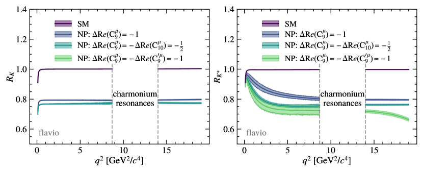
Figure 3: Variation of (left) $R_{K}$ and (right) $R_{{{K}^{*}}}$ as a function of $q^{2}$ within the SM obtained using the flavio software package [71], taking into account potential heavy BSM contributions to the Wilson coefficients. The contributions from ${c}{\overline{c}}$ resonances are subtracted in both cases. For $R_{K}$, the SM prediction overlaps with the BSM scenario $\Delta{\cal R}e(C_{9}^{\mu})=-\Delta{\cal R}e(C_{9}^{\prime\mu})=-1$.

The impact of modifying the muonic $\mathcal{C}_{9}$ and $\mathcal{C}_{10}$ Wilson coefficients on the $R_{K}$ and $R_{{{K}^{*}}}$ LU ratios is illustrated in Fig. 3. The strikingly different $q^{2}$ behavior between the predicted values of $R_{K}$ and $R_{{{K}^{*}}}$ would allow precise measurements to resolve the contributions from the different Wilson coefficients.

4 Analysis strategy

The fundamental approach of this analysis is to treat the measurements of $R_{K}$ and $R_{{{K}^{*}}}$ as null tests of the Standard Model. The analysis is designed to maximize the signal significance at the expected SM decay rates, and achieves a higher signal purity than previous LHCb analyses of these decay modes. The treatment of decays with different final states is also made as coherent as possible, including at the triggering stage. A multivariate selection based on decay kinematics, geometric features and displacement from the associated PV is used to reject combinatorial background. In addition, PID requirements and two dedicated selections, defined later, are designed to suppress backgrounds from other partially reconstructed beauty hadron decays, as well as to improve purity for electron signals in the region below the $b$ hadron masses. Three data-taking periods based on common center-of-mass energies and trigger thresholds are defined and used throughout this analysis: Run 1 (2011–2012), Run 2p1 (2015–2016), and Run 2p2 (2017–2018). Given that many aspects of the analysis depend on the treatment of electron bremsstrahlung, three further categories are defined based on whether the dielectron system has zero, one, or at least two associated bremsstrahlung photons.

The definition of the $\text{central-}{q^{2}}$ region from 1.1 to 6.0$\text{\,Ge\kern-1.00006ptV}^{2}\!/c^{4}$ is the same as in previous LHCb analyses of these decay modes [21, 24]. The lower limit excludes the light meson resonances, while the upper limit minimizes background contamination from resonant ${{J\mskip-3.0mu/\mskip-2.0mu\psi}}\!\rightarrow{e^{+}e^{-}}$ decays that can undergo bremsstrahlung emission, resulting in a reconstructed dilepton invariant mass well below the known ${J\mskip-3.0mu/\mskip-2.0mu\psi}$ mass. The definition of the $\text{low-}{q^{2}}$ region is changed from that used in the previous LHCb measurement of $R_{{{K}^{*}}}$ [21], where it extended down to the dimuon mass threshold of $0.045$$\text{\,Ge\kern-1.00006ptV}^{2}\!/c^{4}$ to increase the signal yield, leading to substantial contamination from the photon pole in the electron mode. This lepton mass effect induces significant LU breaking also within the SM, with an expected $R_{{{K}^{*}}}$ value of $\sim\!0.9$. The current analysis defines the $\text{low-}{q^{2}}$ region from 0.1 to 1.1$\text{\,Ge\kern-1.00006ptV}^{2}\!/c^{4}$, excluding most of the photon pole and leading to an expected $R_{{{K}^{*}}}$ value of $\sim\!0.98$ within the SM [14], close to unity as also expected for the $\text{central-}{q^{2}}$ region. The same definition of the $\text{low-}{q^{2}}$ region is used for $R_{K}$.

As in previous LHCb analyses of LU, the $R_{K}$ and $R_{{{K}^{*}}}$ ratios are measured by forming double ratios of efficiency corrected yields in the nonresonant and resonant modes,

$$R_{(K,{{K}^{*}})} \equiv\frac{\tfrac{\cal{N}}{\varepsilon}({B}^{(+,0)}\!\rightarrow{K}^{(+,*0)}{\mu^{+}\mu^{-}})}{\tfrac{\cal{N}}{\varepsilon}({B}^{(+,0)}\!\rightarrow{K}^{(+,*0)}{{J\mskip-3.0mu/\mskip-2.0mu\psi}}(\!\rightarrow{\mu^{+}\mu^{-}}))}\bigg{/}\frac{\tfrac{\cal{N}}{\varepsilon}({B}^{(+,0)}\!\rightarrow{K}^{(+,*0)}{e^{+}e^{-}})}{\tfrac{\cal{N}}{\varepsilon}({B}^{(+,0)}\!\rightarrow{K}^{(+,*0)}{{J\mskip-3.0mu/\mskip-2.0mu\psi}}(\!\rightarrow{e^{+}e^{-}}))}\,,$$ (2)

where $\tfrac{\cal{N}}{\varepsilon}(X)$ represents the efficiency corrected yield for process $X$. Potential systematic uncertainties arising from differences in the detection efficiencies for muons and electron largely cancel in the double ratios, apart from those induced by kinematic differences between the signal and resonant modes. The single ratios of efficiency corrected yields in the resonant ${J\mskip-3.0mu/\mskip-2.0mu\psi}$ modes,

$$r_{{{J\mskip-3.0mu/\mskip-2.0mu\psi}}}^{K,{{K}^{*}}} \equiv\frac{\tfrac{\cal{N}}{\varepsilon}({B}^{(+,0)}\!\rightarrow{K}^{(+,*0)}{{J\mskip-3.0mu/\mskip-2.0mu\psi}}(\!\rightarrow{\mu^{+}\mu^{-}}))}{\tfrac{\cal{N}}{\varepsilon}({B}^{(+,0)}\!\rightarrow{K}^{(+,*0)}{{J\mskip-3.0mu/\mskip-2.0mu\psi}}(\!\rightarrow{e^{+}e^{-}}))}$$ (3)

are used extensively to perform cross-checks of the analysis procedure, as described in Section 8. Additional cross-checks are performed using two double ratios, $R_{{\psi{(2S)}}}^{{K}}$ and $R_{{\psi{(2S)}}}^{{{K}^{*}}}$, which are defined in direct analogy with Eq. 2, substituting the signal modes with the resonant $\psi{(2S)}$ decays to ${e^{+}}{e^{-}}$ and ${\mu^{+}\mu^{-}}$.

A simultaneous fit to the reconstructed ${B}^{0,+}$ candidate mass distributions in the signal modes and resonant ${J\mskip-3.0mu/\mskip-2.0mu\psi}$ modes is used to determine $R_{K}$ and $R_{{{K}^{*}}}$ within the low and $\text{central-}{q^{2}}$ ranges. This approach allows the $4\times 4$ covariance matrix of statistical and systematic uncertainties to be determined so that they can be incorporated into global fits or alternative interpretations. Partially reconstructed ${{B}^{0}}\!\rightarrow{{K}^{*0}}{e^{+}e^{-}}$ decays, where the pion from the ${{K}^{*0}}\!\rightarrow{{K}^{+}}{{\pi}^{-}}$ decay chain is not selected, represent a significant background in the invariant-mass spectrum of ${{B}^{+}}\!\rightarrow{{K}^{+}}{e^{+}e^{-}}$ decays. The simultaneous fit allows the yield of the partially reconstructed ${K}^{*0}$ $e^{+}e^{-}$ background, as well as contributions from the isospin-related decay ${{B}^{+}}\!\rightarrow{{K}^{*+}}{e^{+}}{e^{-}}$, to be constrained by the fully reconstructed ${{B}^{0}}\!\rightarrow{{K}^{*0}}{e^{+}e^{-}}$ signal and known detector efficiencies. This improves the sensitivity of the fit, and for the first time also ensures that the background yield in the ${K}^{+}$ $e^{+}e^{-}$ spectrum is consistent with the measured value of $R_{{{K}^{*}}}$.

Trigger decisions are associated with particles reconstructed offline. Requirements can be made on whether the decision was due to the reconstructed signal candidate (triggered on signal or TOS); or independent of the signal candidates and due to other particles produced in the ${p}{p}$ collision (triggered independent of signal or TIS); or a combination of both. This analysis divides the events into mutually exclusive categories based on the L0 trigger decision, similar to previous LU tests.

The L0 trigger makes decisions based on kinematic information from the muon and calorimeter systems, with associated quantities having lower resolution and reconstruction efficiency than their offline counterparts. The L0 trigger has a significant fraction of TIS events which can be used for the analysis. As the L0 hadron trigger can have a different performance for ${{K}^{+}}$ and ${K}^{*0}$ final states due to overlapping clusters in the hadronic calorimeter, events exclusively selected by it are excluded from this analysis for both muons and electrons, leading to a negligible loss of efficiency for ${{B}^{0}}\!\rightarrow{{K}^{*0}}{e^{+}e^{-}}$ decays and up to 14% for ${{B}^{+}}\!\rightarrow{{K}^{+}}{e^{+}e^{-}}$ decays. In the case of muon signals, over 90% of events selected by the L0 trigger are TOS, and only around 25% are TIS (the excess in the sum over 100% is due to some events being both TOS and TIS). Due to larger background rates, the L0 electron trigger has more stringent requirements and a lower signal efficiency than the muon trigger. As a result, the TOS fraction is only around 60%, while the TIS fraction is around 50%. Even though the fraction of muon TIS is small, the overall detector efficiency for muons is much larger than for electrons. Therefore, the absolute yield of muon TIS is still larger than that of electron signals in either the TIS or TOS categories.

In order to define mutually exclusive samples, the primary trigger category is chosen to be TIS for both muon and electron final states. Events that are TOS on the L0 muon or electron trigger, whilst being not TIS (i.e. they are not in the primary trigger category), are placed into the secondary trigger category for muon and electron final states, respectively. This approach has several advantages compared to that used in previous LHCb LU analyses where the L0 hadron trigger on the ${K}^{+}$ and ${K}^{*0}$ candidates was used and preference to TOS category was given. Firstly, it increases the muon signal yields and gives two almost equally populated trigger categories for electron signals. Secondly, although trigger decisions due to the signal candidate are directly correlated with kinematic quantities, trigger decisions due to the rest of the ${p}{p}$ collision only modify the signal kinematics indirectly; this occurs through correlations between the signal and other particles produced in the same ${p}{p}$ collision. The TIS category therefore not only minimizes efficiency differences between the muon and electron signals, but also minimizes the impact of differences in the signal kinematics between data and simulation.

The HLT selects events based on tracking information, with loose lepton identification requirements also applied. It is therefore sufficiently well aligned with the offline selection not to require any special treatment beyond the choice of appropriate trigger paths for the electron and muon modes described earlier. Only a few percent of events are TIS at the HLT stage. These HLT-TIS events are crucial for calibrating the TOS trigger performance in data as described in Sec. 6, but are not otherwise used in the analysis (unless they are also TOS).

5 Event selection and background

The reconstruction of ${{B}^{+}}\!\rightarrow{{K}^{+}}{\ell^{+}}{\ell^{-}}$ and ${{B}^{0}}\!\rightarrow{{K}^{*0}}{\ell^{+}}{\ell^{-}}$ candidates requires a dilepton system, which consists of a pair of oppositely charged particles, identified as either electrons or muons and required to originate from a common vertex. Muons and electrons are required to have $p_{\mathrm{T}}$ greater than 800 and 500$\text{\,Me\kern-1.00006ptV\!/}c$, respectively, and to have momentum greater than 3$\text{\,Ge\kern-1.00006ptV\!/}c$. All tracks used in this analysis are required to satisfy track quality requirements, using their $\chi^{2}$ as determined by a Kalman filter and the output of a neural network trained to distinguish between genuine and fake tracks [72]. A dedicated algorithm associates reconstructed bremsstrahlung photons to tracks identified as electrons; when a given photon is associated with both electron tracks, it is attached to one chosen randomly. The bremsstrahlung energy loss recovery procedure is used to improve the electron momentum resolution by searching for photon clusters that are not already associated with particle tracks in the event. This takes place within regions in the electromagnetic calorimeters into which electron tracks segments reconstructed upstream of the magnet have been extrapolated. Lepton tracks and dilepton candidates are required to satisfy criteria on transverse momenta, displacement from the PV and, for dilepton candidates, their vertex fit quality. A similar approach is used to reconstruct ${{K}^{*0}}\!\rightarrow{{K}^{+}}{{\pi}^{-}}$ candidates. The $B$ candidates are subsequently formed by combining the dilepton candidates with either a charged particle identified as a ${K}^{+}$, or with the ${K}^{*0}$ candidates for which the invariant mass of the $K$ $\pi$ system is required to be within 100$\text{\,Me\kern-1.00006ptV\!/}c^{2}$ of the known ${K}^{*0}$ mass [51]. The $B$ candidates need to satisfy minimal criteria on their transverse momentum, displacement from the PV and vertex fit quality. The fit of the $B$ candidate is performed using the decay tree fitter [73] algorithm. In addition, the $B$-candidate momentum vector is required to be consistent with the vector connecting the $B$ candidate’s production and decay vertices (the displacement vector).

Minimum requirements on the angles between final-state particle trajectories ensure that the $B$ candidates are not constructed from duplicated tracks using the same track segment in the vertex detector. The criteria applied in this reconstruction and preselection are identical for the signal and resonant control modes, and are aligned as much as possible between the ${K}^{+}$ and ${K}^{*0}$ final states. Finally, the $B$ candidates are divided into regions based on their reconstructed dilepton $q^{2}$:

$$\text{low-}{q^{2}} 0.1<{q^{2}}<1.1\text{\,Ge\kern-1.00006ptV}^{2}\!/c^{4}\,,$$ region:

$$\text{central-}{q^{2}} 1.1<{q^{2}}<6.0\text{\,Ge\kern-1.00006ptV}^{2}\!/c^{4}\,,$$ region:

electron $${J\mskip-3.0mu/\mskip-2.0mu\psi} 6<{q^{2}}<11\text{\,Ge\kern-1.00006ptV}^{2}\!/c^{4}\,,$$ region:

muon $${J\mskip-3.0mu/\mskip-2.0mu\psi} |m({\ell^{+}}{\ell^{-}})-M_{{{J\mskip-3.0mu/\mskip-2.0mu\psi}}}^{\mathrm{PDG}}|<100\text{\,Me\kern-1.00006ptV\!/}c^{2}\,,$$ region:

electron $$\psi{(2S)} 11<{q^{2}}<15\text{\,Ge\kern-1.00006ptV}^{2}\!/c^{4}\,,$$ region:

muon $$\psi{(2S)} |m({\ell^{+}}{\ell^{-}})-M_{{\psi{(2S)}}}^{\mathrm{PDG}}|<100\text{\,Me\kern-1.00006ptV\!/}c^{2}\,,$$ region:

where $M_{{{J\mskip-3.0mu/\mskip-2.0mu\psi}}}^{\mathrm{PDG}}$ and $M_{{\psi{(2S)}}}^{\mathrm{PDG}}$ are the known masses of the ${J\mskip-3.0mu/\mskip-2.0mu\psi}$ and $\psi{(2S)}$ mesons [51], respectively. The low- and $\text{central-}{q^{2}}$ regions are identical for muons and electrons, whereas the resonant regions are significantly broader for electrons due to their poorer dilepton mass resolution.

Particle identification requirements are used to suppress backgrounds. Two families of variables are used: the difference in log-likelihood between the given charged-species hypothesis and the pion hypothesis (named DLL), and the output of artificial neural networks trained to identify each charged-particle species (normalized between 0 and 1 and named ProbNN) [74, 28, 47]. The multivariate approach uses information from all subdetectors to compute the compatibility of each track with a given particle hypothesis. Muons and electrons are required to satisfy stringent compatibility criteria with their assigned particle hypothesis. Kaons and pions must satisfy both a minimal compatibility requirement with their assigned particle hypothesis and be incompatible with an alternative hypothesis. The alternative hypotheses considered are protons in the case of kaon candidates, and protons and kaons in the case of pion candidates. Kaons and electrons are required to satisfy minimal criteria with respect to the pion hypothesis.

As PID requirements are calibrated using data from control samples as discussed in Section 6, further kinematic and geometric fiducial requirements are necessary to align the selection of tracks in the candidates with those in the control samples. Wherever possible the same requirements are applied to the resonant control modes. This reduces potential systematic uncertainties associated with the determination of relative selection efficiencies in the $R_{K}$ and $R_{{{K}^{*}}}$ double ratios. While PID criteria factorize for most particle species, an electron-positron pair can have correlated PID efficiencies due to overlapping clusters in the ECAL. Therefore, as discussed in Sec. 6.1, a fiducial requirement is used to remove such candidates from the analysis. Although the preselection and PID requirements achieve acceptable purity for the resonant control modes, further selection requirements are essential to improve the purity of the signal modes.

The remaining backgrounds are divided into four groups: random combinations of particles originating from multiple physical sources (combinatorial); backgrounds having missing energy in which all particles originate from a single physical process (partially reconstructed); individual backgrounds that are vetoed with specific criteria or taken into account in the invariant mass fit (exclusive); and residual backgrounds from hadrons misidentified as electrons, with or without missing energy, that must be taken into account in the invariant mass fit (misidentified). With the application of all criteria, less than one percent of events have multiple candidates; in such cases a single reconstructed candidate is chosen randomly.

5.1 Combinatorial and partially reconstructed backgrounds

A multivariate classifier [75, 76] is trained to distinguish between $B^{(+,0)}\!\rightarrow K^{(+,*0)}{\ell^{+}}{\ell^{-}}$ decays and combinatorial background. The training uses simulated signal events, and data with reconstructed $B$ meson invariant masses above 5400 (5600)$\text{\,Me\kern-1.00006ptV\!/}c^{2}$ as a proxy for the muon (electron) combinatorial background. Background events are combined for the low- and $\text{central-}{q^{2}}$ regions to increase the size of the training samples. The full set of preselection and PID requirements are applied to the data before training, for which the same number of signal and background events are used. Separate classifiers are trained for the Run 1, Run 2p1, and Run 2p2 data-taking periods. Ten different classifiers are trained for each period, using a k-fold cross-validation approach to avoid biases [77] in which each of the ten classifiers is trained leaving out a different 10% of the data sample. The list of classifier inputs is reduced by repeating the training, excluding inputs sequentially and retaining only those whose inclusion increases the area under the ROC (Receiver Operating Characteristic) curve by at least 1%. The same inputs are used for all three run periods.

The response of the multivariate classifier is verified to have no significant correlation with the $B$ candidate mass. The final set of inputs is based on the following features of the candidates:

$B$

transverse momentum, vertex fit quality, displacement from the PV, compatibility of momentum and displacement vectors;

$\ell^{+}\ell^{-}$

transverse momentum, vertex fit quality, displacement from the PV;

${K}^{+}$, ${K}^{*0}$

transverse momentum, displacement from the PV;

Leptons

minimum and maximum transverse momentum and displacement of the two leptons from the PV;

${{K}^{*0}}\!\rightarrow{{K}^{+}}{{\pi}^{-}}$ final state hadrons

minimum and maximum transverse momentum and displacement of the two hadrons.

Partially reconstructed backgrounds are particularly important for the electron final states as bremsstrahlung leads to missing energy even in the case of correctly reconstructed candidates, introducing a significant overlap of signal and backgrounds. A dedicated classifier is therefore trained for the electron modes to distinguish between $B^{(+,0)}\!\rightarrow K^{(+,*0)}{e^{+}e^{-}}$ signal decays and partially reconstructed backgrounds. In this case, a phase space simulation of ${{B}^{+}}\!\rightarrow{{K}^{+}}{{\pi}^{+}}{{\pi}^{-}}{e^{+}e^{-}}$ is used as proxy for partially reconstructed background in ${{B}^{0}}\!\rightarrow{{K}^{*0}}{e^{+}e^{-}}$ decays, while simulated ${{B}^{0}}\!\rightarrow{{K}^{*0}}{e^{+}e^{-}}$ decays serve as a background proxy for ${{B}^{+}}\!\rightarrow{{K}^{+}}{e^{+}e^{-}}$ decays. The training follows the same procedure as used for the combinatorial classifier. In addition to observables that describe the kinematic and geometric properties of the decays, isolation variables, such as the track multiplicity and the vertex quality obtained adding extra tracks from the underlying event to the reconstructed vertex, are evaluated. Only tracks from the underlying event contained within a cone defined by $\sqrt{(\eta-\eta_{B})^{2}+(\phi-\phi_{B})^{2})}<0.5$ are considered, where $\eta_{B}$ and $\phi_{B}$ are the pseudorapidity and the azimuthal angle (given in radians) relative to the beam direction of the reconstructed $B$ candidate, respectively. Such variables contribute significantly to the rejection of candidates originating from partially reconstructed decay processes. These isolation variables consider the multiplicity of particles other than the $B$ candidate within this cone, the scalar sum of their transverse momenta and the fraction of transverse momentum within the cone attributed to the $B$ candidate. A further set of isolation variables is computed by sequentially adding other tracks in the event to the $B$ candidate vertex and computing the mass of this new candidate vertex. The obtained vertex $\chi^{2}$ is used to define which new candidate vertex is most similar to that of the original $B$ candidate vertex. The $\chi^{2}$ and invariant mass of this vertex are retained for use in the classifier to reject partially reconstructed backgrounds.

The classifiers developed to reduce combinatorial and partially reconstructed backgrounds are optimized using the expected signal significance $N_{\textrm{S}}/\sqrt{N_{\textrm{S}}+N_{\textrm{B}}}$ as a figure of merit, where $N_{\textrm{S}}$ and $N_{\textrm{B}}$ represent the expected numbers of signal and background events within signal intervals defined as $\pm 50\text{\,Me\kern-1.00006ptV\!/}c^{2}$ around the known $B$ meson mass [51] for muon modes and, to account for bremsstrahlung, 5150–5350$\text{\,Me\kern-1.00006ptV\!/}c^{2}$ for electron modes. Here $N_{\textrm{S}}$ is obtained from simulated samples of resonant ${J\mskip-3.0mu/\mskip-2.0mu\psi}$ decays, normalized to the measured yields in data with no selections applied on the classifiers. It is scaled by the SM expectation for the ratios of nonresonant and resonant branching fractions, computed using flavio package [71], as well as the ratio of efficiencies between the nonresonant and resonant modes at the respective working points of the classifiers. The expected number of combinatorial background events in the signal window, $N_{\textrm{B}}$, is obtained from simplified fits to samples of data candidates passing the preselection and PID requirements.

A one-dimensional optimization of the combinatorial classifier response is performed for muon signals, while a two-dimensional optimization of the combinatorial and partially reconstructed classifier response is performed for the electron signals. The classifiers for the low- and $\text{central-}{q^{2}}$ regions in each run period are optimized separately. It is verified that the classifiers do not sculpt the reconstructed $B$ meson mass lineshape and $q^{2}$ spectrum, and the optimal working points are located on broad plateaus of signal significance in all cases. Analogous optimizations are performed for the ${J\mskip-3.0mu/\mskip-2.0mu\psi}$ and $\psi{(2S)}$ resonant control modes, with appropriate adjustments to take into account their different backgrounds. A single set of combinatorial and partially reconstructed classifier response criteria is chosen for all electron signals and resonant muon modes, while muon signals and resonant electron modes are selected using a different set of classifier response criteria for each run period.

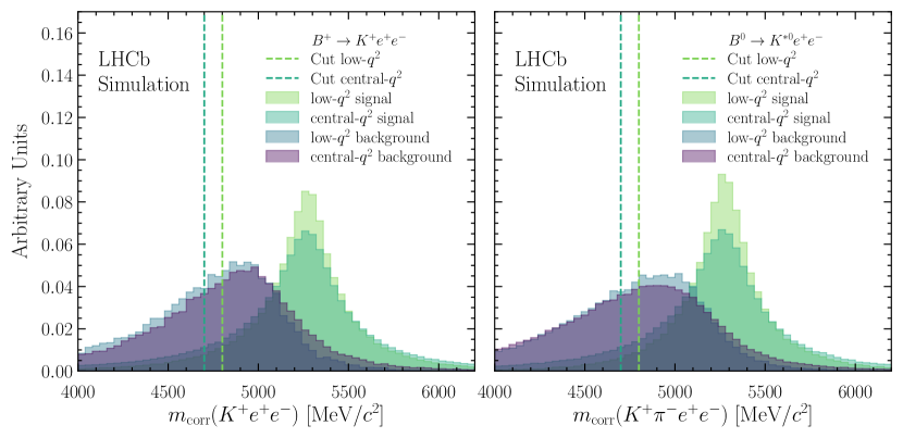
Figure 4: Distribution of $m_{\mathrm{corr}}$ for the simulated (left) ${{B}^{+}}\!\rightarrow{{K}^{+}}{e^{+}e^{-}}$ and (right) ${{B}^{0}}\!\rightarrow{{K}^{*0}}{e^{+}e^{-}}$ candidates after applying the nominal analysis criteria to the response of the combinatorial and partially reconstructed multivariate classifiers. The distributions of the signal in the low- and $\text{central-}{q^{2}}$ regions and the partially reconstructed background are shown (unit normalizations). The ${B}^{+}$ and ${B}^{0}$ partially reconstructed backgrounds are taken from simulated ${{B}^{0}}\!\rightarrow{{K}^{*0}}{e^{+}e^{-}}$ and ${{B}^{+}}\!\rightarrow{{K}^{+}}{{\pi}^{+}}{{\pi}^{-}}{e^{+}e^{-}}$ decays, respectively. The vertical lines show the selection requirements applied for the two signal regions.

Partially reconstructed backgrounds in electron modes are further suppressed by using the ratio of the hadronic and dielectron momentum components transverse to the $B$ direction of flight to correct the momentum of the dielectron pair [21]. In the approximation that the dielectron direction is not modified significantly, this ratio is expected to be unity unless electrons have lost energy due to bremsstrahlung that is not recovered. The invariant mass calculated using the corrected dielectron momentum, $m_{\mathrm{corr}}$, has significant power to distinguish between signals and backgrounds that satisfy the nominal combinatorial and partially reconstructed classifier criteria, as illustrated in Fig. 4. The $m_{\mathrm{corr}}$ criteria are optimized in a similar manner to the multivariate classifiers and are applied after them to reduce further combinatorial and partially reconstructed backgrounds. Since the $m_{\mathrm{corr}}$ criteria sculpt the combinatorial background, potential biases introduced by them are considered as a source of systematic uncertainty.

5.2 Exclusive backgrounds

Dedicated simulated event samples are used to study backgrounds which remain after all previously described selection criteria have been applied. Specific vetoes are used to reduce many of these backgrounds to a negligible level. To ensure high efficiency for the signal, stronger PID requirements are imposed in the mass interval close to a resonance rather than applying a veto on invariant mass only. It is necessary to evaluate these backgrounds and vetoes separately for the ${{B}^{+}}\!\rightarrow{{K}^{+}}{\ell^{+}}{\ell^{-}}$ and ${{B}^{0}}\!\rightarrow{{K}^{*0}}\ell^{+}\ell^{-}$ decay modes.

For ${{B}^{+}}\!\rightarrow{{K}^{+}}{\ell^{+}}{\ell^{-}}$ decays, the residual backgrounds accounted for in the fits are summarized in Table 1 and additional selection criteria are applied to suppress background contributions from:

${{B}^{+}}\!\rightarrow({{\kern 1.79993pt\overline{\kern-1.79993ptD}}{}^{0}}\!\rightarrow{{K}^{+}}{{\pi}^{-}}){\ell^{+}}{{\nu}_{\ell}}$:

This decay has one pion misidentified as a charged lepton. If the invariant mass of the kaon and oppositely charged lepton, computed assigning the pion mass hypothesis to the lepton, differs from the known ${D}^{0}$ mass [51] by less than 40$\text{\,Me\kern-1.00006ptV\!/}c^{2}$, the charged lepton must satisfy tighter PID requirements. This background affects all $q^{2}$ regions.

${{B}^{+}}\!\rightarrow({{\kern 1.79993pt\overline{\kern-1.79993ptD}}{}^{0}}\!\rightarrow{{K}^{+}}{\ell^{-}}{{\overline{\nu}}_{\ell}})$ $\ell^{+}$ ${\nu}_{\ell}$:

This decay has two additional neutrinos compared to the signal mode resulting in significant missing energy. To suppress this background, the invariant mass of the kaon and the lepton with opposite charge to the kaon is required to be greater than 1780$\text{\,Me\kern-1.00006ptV\!/}c^{2}$ as illustrated in Fig. 5. This background affects the low- and $\text{central-}{q^{2}}$ regions.

Hadron-lepton swap:

This background involves a double misidentification which may cause a resonant mode candidate to be misidentified as signal since the overall invariant mass of the ${{K}^{+}}\ell^{+}\ell^{-}$ system still peaks in the vicinity of the ${{B}^{+}}$ meson mass while the reconstructed dilepton mass is mistakenly different from the charmonium mass. In the muon mode, where the invariant mass of the system formed by the kaon (under the muon mass hypothesis) and the oppositely charged muon differ by less than 60$\text{\,Me\kern-1.00006ptV\!/}c^{2}$ from the known masses of the ${J\mskip-3.0mu/\mskip-2.0mu\psi}$ and $\psi{(2S)}$ mesons, the muon is required to satisfy stringent PID criteria. In the electron mode, the ${{K}^{+}}\ell^{+}\ell^{-}$ invariant mass is recomputed swapping the kaon and same-charge electron mass hypotheses and constraining the invariant mass of the dilepton system to the ${J\mskip-3.0mu/\mskip-2.0mu\psi}$ or $\psi{(2S)}$ masses. Where this ${{K}^{+}}\ell^{+}\ell^{-}$ mass differs by less than 60$\text{\,Me\kern-1.00006ptV\!/}c^{2}$ from the known ${{B}^{+}}$ mass, the electron is required to satisfy stringent electron identification criteria. This background affects all $q^{2}$ regions.

${{{B}^{+}}}\!\rightarrow{\psi{(2S)}}(\!\rightarrow{{J\mskip-3.0mu/\mskip-2.0mu\psi}}X){{K}^{+}}$:

The invariant mass of the reconstructed ${{B}^{+}}$ candidate is required to be at least 200 $\text{\,Me\kern-1.00006ptV\!/}c^{2}$ greater than the ${{B}^{+}}$ meson mass when the dilepton mass is constrained to the known $\psi{(2S)}$ meson mass. This background affects the ${J\mskip-3.0mu/\mskip-2.0mu\psi}$ region.

Table 1: Exclusive backgrounds modeled in the ${{B}^{+}}\!\rightarrow{{K}^{+}}{\ell^{+}}{\ell^{-}}$ invariant mass fits, along with the $q^{2}$ region of interest and the mode(s) for which the background is relevant.

Decay mode	$q^{2}$ region	Relevant mode(s)
${{B}^{+}}\!\rightarrow{{\pi}^{+}}{{J\mskip-3.0mu/\mskip-2.0mu\psi}}(\!\rightarrow{\ell^{+}}{\ell^{-}})$	${J\mskip-3.0mu/\mskip-2.0mu\psi}$	electron and muon
${{B}^{0}_{s}}\!\rightarrow{{\kern 1.79993pt\overline{\kern-1.79993ptK}}{}^{*0}}{{J\mskip-3.0mu/\mskip-2.0mu\psi}}(\!\rightarrow{\ell^{+}}{\ell^{-}})$	${J\mskip-3.0mu/\mskip-2.0mu\psi}$	electron and muon
${{B}^{0}}\!\rightarrow{{K}^{*0}}{\psi{(2S)}}(\rightarrow{\ell^{+}}{\ell^{-}})$	$\psi{(2S)}$	electron and muon
$B^{+,0}\rightarrow(K\pi)^{+,0}\ell\ell$	low/central	electron

For ${{B}^{0}}\!\rightarrow{{K}^{*0}}{\ell^{+}}{\ell^{-}}$ decays, the residual backgrounds accounted for in the fits are summarized in Table 2 and additional selection criteria are applied to suppress background contributions from:

${{B}^{0}_{s}}\!\rightarrow\phi(1020)\ell^{+}\ell^{-}$:

This decay has one kaon misidentified as a pion. Where the ${K}^{+}$ ${\pi}^{-}$ invariant mass, recomputed under the ${K}^{+}$ ${K}^{-}$ mass hypothesis, is less than 1040$\text{\,Me\kern-1.00006ptV\!/}c^{2}$, the pion is required to satisfy stringent PID criteria. This background affects all $q^{2}$ regions and can only be fully vetoed in the low- and central-$q^{2}$ regions. In the resonant modes a non-negligible amount of this background remains after the veto and is modeled in the fits.

${{B}^{0}}\!\rightarrow({{\kern 1.79993pt\overline{\kern-1.79993ptD}}{}^{0}}\!\rightarrow{{K}^{+}}{{\pi}^{-}}){{\pi}^{-}}{\ell^{+}}{{\nu}_{\ell}}$:

This decay has one pion misidentified as a charged lepton and one neutrino compared to the signal mode. Where the invariant mass of the kaon and oppositely charged lepton, computed by assigning the pion mass hypothesis to the lepton, differs by less than 30$\text{\,Me\kern-1.00006ptV\!/}c^{2}$ from the known ${D}^{0}$ meson mass, the lepton is required to satisfy stringent PID criteria. This background affects all $q^{2}$ regions;

${{B}^{0}}\!\rightarrow({{D}^{-}}\!\rightarrow({{K}^{*0}}\!\rightarrow{{K}^{+}}{{\pi}^{-}}){{\pi}^{-}}){\ell^{+}}{{\nu}_{\ell}}$:

If the invariant mass of the ${K}^{+}$ ${\pi}^{-}$ system and the lepton with opposite charge to the kaon (computed under the pion mass hypothesis) differs by less than 30$\text{\,Me\kern-1.00006ptV\!/}c^{2}$ from the known ${D}^{-}$ meson mass, the lepton is required to satisfy stringent PID criteria. This background affects all $q^{2}$ regions.

${{B}^{0}}\!\rightarrow({{D}^{-}}\!\rightarrow({{K}^{*0}}\!\rightarrow{{K}^{+}}{{\pi}^{-}}){\ell^{-}}{{\overline{\nu}}_{\ell}}){\ell^{+}}{{\nu}_{\ell}}$ :

This decay differs from the signal mode by having two additional neutrinos in the final state. The invariant mass of the ${K}^{+}$ ${\pi}^{-}$ system and the lepton with opposite charge with respect to the kaon is required to be greater than 1780$\text{\,Me\kern-1.00006ptV\!/}c^{2}$ as illustrated in Fig. 5. This background affects the low- and $\text{central-}{q^{2}}$ regions.

${{{B}^{+}}}\!\rightarrow{{K}^{+}}\ell^{+}\ell^{-}$:

This decay, with the addition of a random pion from the underlying event can constitute a background for the ${{B}^{0}}\!\rightarrow{{K}^{*0}}{\ell^{+}}{\ell^{-}}$ candidates. This background is suppressed applying an invariant mass requirement to the ${{\pi}^{-}}\ell^{+}\ell^{-}$ system, assigning the kaon mass hypothesis to the pion, and to the invariant mass of the ${{K}^{+}}\ell^{+}\ell^{-}$ system. Both the invariant masses for a given ${{B}^{0}}\!\rightarrow{{K}^{*0}}{\ell^{+}}{\ell^{-}}$ candidate are required to be smaller than 5100$\text{\,Me\kern-1.00006ptV\!/}c^{2}$. This background affects all $q^{2}$ regions.

Hadron-lepton swap:

This background has the same physical origin as, and is treated analogously to, its counterpart in the ${{B}^{+}}$ decay.

${{B}^{0}}\!\rightarrow{\psi{(2S)}}(\!\rightarrow{{J\mskip-3.0mu/\mskip-2.0mu\psi}}X){{K}^{*0}}$:

This background also has the same physical origin as, and is treated analogously to, its counterpart in the ${{B}^{+}}$ decay.

Table 2: Exclusive backgrounds modeled in the ${{B}^{0}}\!\rightarrow{{K}^{*0}}\ell^{+}\ell^{-}$ invariant mass fits, the $q^{2}$ region of interest and the mode(s) for which the background is relevant. The $K-\pi$ swap backgrounds refer to cases where the mass hypotheses of the kaon and pion from a genuine ${{B}^{0}}\!\rightarrow{{K}^{*0}}\ell^{+}\ell^{-}$ decay are swapped.

Decay mode	$q^{2}$ region	Relevant mode(s)
${{B}^{0}_{s}}\!\rightarrow{{\kern 1.79993pt\overline{\kern-1.79993ptK}}{}^{*0}}{{J\mskip-3.0mu/\mskip-2.0mu\psi}}(\!\rightarrow{\ell^{+}}{\ell^{-}})$	${J\mskip-3.0mu/\mskip-2.0mu\psi}$	electron and muon
${{B}^{0}_{s}}\!\rightarrow\phi(1020){{J\mskip-3.0mu/\mskip-2.0mu\psi}}(\!\rightarrow{\ell^{+}}{\ell^{-}})$	${J\mskip-3.0mu/\mskip-2.0mu\psi}$	electron and muon
${{\mathchar 28931\relax}^{0}_{b}}\!\rightarrow p{{K}^{-}}{{J\mskip-3.0mu/\mskip-2.0mu\psi}}(\!\rightarrow{\ell^{+}}{\ell^{-}})$	${J\mskip-3.0mu/\mskip-2.0mu\psi}$	electron and muon
${B}\!\rightarrow X{{J\mskip-3.0mu/\mskip-2.0mu\psi}}(\!\rightarrow{\ell^{+}}{\ell^{-}})$	${J\mskip-3.0mu/\mskip-2.0mu\psi}$	electron and muon
$K-\pi$ swap	${J\mskip-3.0mu/\mskip-2.0mu\psi}$	electron and muon
${{B}^{0}_{s}}\!\rightarrow{{\kern 1.79993pt\overline{\kern-1.79993ptK}}{}^{*0}}{\psi{(2S)}}(\!\rightarrow{\ell^{+}}{\ell^{-}})$	$\psi{(2S)}$	electron and muon
${{\mathchar 28931\relax}^{0}_{b}}\!\rightarrow p{{K}^{-}}\psi(2S)(\!\rightarrow{\ell^{+}}{\ell^{-}})$	$\psi{(2S)}$	electron and muon
${B}\!\rightarrow X{\psi{(2S)}}(\!\rightarrow{\ell^{+}}{\ell^{-}})$	$\psi{(2S)}$	electron and muon
$K-\pi$ swap	$\psi{(2S)}$	electron and muon
$B^{+,0}\!\rightarrow(K\pi\pi)^{+,0}\ell^{+}\ell^{-}$	low/central	electron

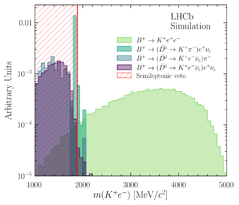
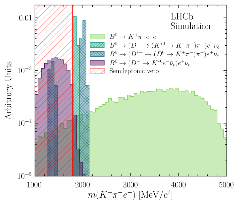
Figure 5: Simulated distributions of (left) $m({{K}^{+}}{e^{-}})$ for ${{B}^{+}}$ candidates and (right) $m({{K}^{+}}{{\pi}^{-}}{e^{-}})$ for ${B}^{0}$ candidates. Signal and various semileptonic cascade backgrounds are shown. The full selection is applied except for the semileptonic background vetos. The hatched areas show decay modes that are also vetoed, recomputing $m({{K}^{+}}{e^{-}})$ and $m({{K}^{+}}{{\pi}^{-}}{e^{-}})$ while assigning the pion mass hypothesis to the electron and not accounting for bremsstrahlung corrections.

Figure 6: Upper: signal efficiencies and background rejection factors for all vetos against physical backgrounds, for (left) ${{B}^{+}}$ and (right) ${B}^{0}$ modes, in the $\text{low-}{q^{2}}$ region; lower: analogous plots for the $\text{central-}{q^{2}}$ region.

The residual contamination of exclusive backgrounds in the low- and $\text{central-}{q^{2}}$ signal regions is evaluated using large samples of simulated background events (Fig. 6). Backgrounds that would form a peaking structure in the $B$ invariant mass, such as ${{B}^{0}_{s}}\!\rightarrow\phi(1020)\ell^{+}\ell^{-}$ or ${{\mathchar 28931\relax}^{0}_{b}}\!\rightarrow{p}{{K}^{-}}\ell^{+}\ell^{-}$, are found to have yields at a few per mille of the expected signal yield, and are therefore considered negligible. Due to their large branching fractions, double-semileptonic decays of the form ${{B}^{0}}\!\rightarrow({{D}^{-}}\!\rightarrow{{K}^{*0}}{e^{-}}{{\overline{\nu}}_{e}}){e^{+}}{{\nu}_{e}}$ are found to have yields of a few percent of the expected signal yield. Since the selection efficiency for these decays is very small, modeling them with dedicated templates in the invariant-mass fit would require prohibitively large simulated event samples to be generated. As these decays involve two neutrinos and significant missing energy they do not form a peaking structure near the invariant mass signal region. They are therefore not modeled explicitly but rather absorbed by other, larger, missing energy background components in the invariant-mass fit.

5.3 Misidentified backgrounds

After applying all selection criteria, a significant contribution from backgrounds in which one or more hadrons are misidentified as leptons, with or without additional missing energy, still remains. These backgrounds have various impacts on the invariant mass fit. Fully reconstructed misidentified decays of the type ${{{B}^{+}}}\!\rightarrow{{K}^{+}}h_{1}h_{2}$ and ${{B}^{0}}\!\rightarrow{{K}^{*0}}h_{1}h_{2}$, where $h_{1,2}$ are kaons or pions, create clear peaking structures in both the electron and muon invariant-mass fits. There are however also numerous backgrounds specific to the electron final states which feature a combination of either single or double misidentification, as well as missing energy. These backgrounds create more complex structures.

One specific example is the decay ${{B}^{0}}\!\rightarrow{{K}^{+}}{{\pi}^{-}}({{\pi}^{0}}\!\rightarrow{e^{+}}{e^{-}}\gamma)$, where the electron from the ${{\pi}^{0}}$ decay is missed, the photon is missed or reconstructed as bremsstrahlung, and the negatively charged pion is misidentified as an electron. This example is similar to the backgrounds discussed in Ref. [78], with a misidentified hadron substituted for one of the electrons. More generally, however, any decay of the type ${{{B}^{+}}}\!\rightarrow{{K}^{+}}{{\pi}^{-}}({{\pi}^{0}},\gamma)X$ or ${{B}^{0}}\!\rightarrow{{K}^{*0}}{{\pi}^{-}}({{\pi}^{0}},\gamma)X$, where $X$ is any number of other final state particles, can contribute. Not all particles from such processes are used to reconstruct the signal, therefore such backgrounds are characterized by low invariant masses.

Compared to previous LU measurements at LHCb, the tighter PID requirements used for electrons reduces the expected rates for pions and kaons to be misidentified as electrons. Table 3 compares the misidentification rates at the working point used in this analysis to those from Ref. [24], for each of the three data taking periods considered. The misidentification rates are determined from data using ${{D}^{*+}}\!\rightarrow{{D}^{0}}(\rightarrow{{K}^{-}}{{\pi}^{+}}){{\pi}^{+}}$ decays. It is noted that in Run 1 a similar pion-to-electron misidentification rate is found from this data-driven method, while a factor two suppression is achieved for kaon-to-electron misidentification. For Run 2p1 and Run 2p2, the pion-to-electron misidentification rates are reduced by a factor two and the kaon-to-electron misidentification rates are reduced by almost a factor of ten; Run 2p1 and Run 2p2 rates are found to be consistent with one another. Table 4 shows the impact of the tighter PID requirements on the overall electron mode signal efficiencies, separated by data-taking period and trigger category. The improved background reduction has only a small impact on the signal efficiencies: in Run 1 these are unchanged, while in Run 2, they are reduced by around 10%.

Table 3: Single-particle misidentification rates obtained on data averaging over the kinematics of prompt $D^{\ast+}\rightarrow D^{0}(\rightarrow K^{-}\pi^{+})\pi^{+}$ decays. The misidentification rates are evaluated for the PID criteria used in this analysis given the acceptance and kinematic requirements applied in the track final state. The misidentification rates corresponding to the PID requirements of Ref. [24] are given in parentheses.

Sample	$\pi\rightarrow e$	$K\rightarrow e$
Run 1p1	$1.78\,(1.70)\,\%$	$0.69\,(1.24)\,\%$
Run 2p1	$0.83\,(1.51)\,\%$	$0.18\,(1.25)\,\%$
Run 2p2	$0.80\,(1.50)\,\%$	$0.16\,(1.23)\,\%$

Table 4: Overall signal efficiency for electron mode in percent. The impact of global event cuts on the efficiency determination is not included as it cancels in the $R_{(K,{{K}^{*}})}$ ratio defined in Eq. (2). The efficiency values obtained applying the same PID requirements of Ref. [24] are given in parentheses.

Sample	${{B}^{+}}\!\rightarrow{{K}^{+}}{e^{+}e^{-}}$		${{B}^{0}}\!\rightarrow{{K}^{*0}}{e^{+}e^{-}}$
	$\text{low-}{q^{2}}$	$\text{central-}{q^{2}}$	$\text{low-}{q^{2}}$	$\text{central-}{q^{2}}$
Run 1p1 $\textrm{TIS\phantom{O}}_{\textrm{\phantom{inc}}}$	$0.152$ ($0.152$)%	$0.138$ ($0.140$)%	$0.054$ ($0.054$)%	$0.051$ ($0.051$)%
Run 1p1 $\textrm{TOS\phantom{I}}_{\textrm{\phantom{inc}}}$	$0.126$ ($0.127$)%	$0.127$ ($0.127$)%	$0.044$ ($0.044$)%	$0.044$ ($0.044$)%
Run 2p1 $\textrm{TIS\phantom{O}}_{\textrm{\phantom{inc}}}$	$0.250$ ($0.273$)%	$0.230$ ($0.252$)%	$0.084$ ($0.092$)%	$0.087$ ($0.095$)%
Run 2p1 $\textrm{TOS\phantom{I}}_{\textrm{\phantom{inc}}}$	$0.239$ ($0.258$)%	$0.228$ ($0.247$)%	$0.074$ ($0.080$)%	$0.081$ ($0.087$)%
Run 2p2 $\textrm{TIS\phantom{O}}_{\textrm{\phantom{inc}}}$	$0.256$ ($0.285$)%	$0.232$ ($0.260$)%	$0.086$ ($0.094$)%	$0.084$ ($0.095$)%
Run 2p2 $\textrm{TOS\phantom{I}}_{\textrm{\phantom{inc}}}$	$0.228$ ($0.253$)%	$0.226$ ($0.249$)%	$0.079$ ($0.086$)%	$0.078$ ($0.087$)%

It is essential to establish whether a significant number of misidentified background candidates pass the full selection criteria, and whether they create distinctive invariant mass distributions that cannot be absorbed by combinatorial or other background components. This task is complicated by the fact that there is a very large number of such backgrounds, many of which are poorly known. Even where the branching fractions of individual ${{{B}^{+}}}\!\rightarrow{{K}^{+}}{{\pi}^{-}}({{\pi}^{0}},\gamma)X$ or ${{B}^{0}}\!\rightarrow{{K}^{*0}}{{\pi}^{-}}({{\pi}^{0}},\gamma)X$ decays have been measured, their Dalitz structure is often unknown. A representative subset of these backgrounds is studied using simulation, and the expected contribution of each individual background found to be negligible. However, even if the contribution of any given background is small, the contribution of all these backgrounds taken together can be large and have a shape that differs from combinatorial background. These considerations lead to a data-driven strategy for modeling the distributions of the residual misidentified backgrounds in this analysis, using control samples enriched with misidentified hadrons. This strategy consists of inverting the stringent lepton identification requirements in the selection, while maintaining the preselection requirements. The resulting dataset (referred to as control region in the following) predominantly contains misidentified background rather than signal candidates and can be used, together with standard PID calibration samples, to estimate the residual misidentified backgrounds.

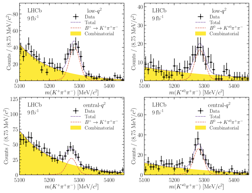
Figure 7: Distributions of the invariant mass of candidates for which both electrons are in the control region, i.e. having the stringent electron identification requirements inverted. The pion mass hypothesis is applied to both electrons, without a bremsstrahlung correction. The left and right columns correspond to the ${{B}^{+}}\!\rightarrow{{K}^{+}}{e^{+}e^{-}}$ and ${{B}^{0}}\!\rightarrow{{K}^{*0}}{e^{+}e^{-}}$ modes, respectively. The upper and lower rows correspond to the low- and $\text{central-}{q^{2}}$ regions, respectively. Fit results are overlaid.

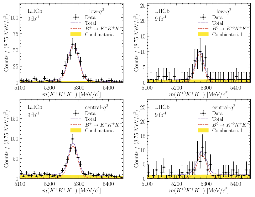
Figure 8: Distributions of the invariant mass of candidates for which both electrons are in the control region, i.e. having the stringent electron identification requirements inverted. The kaon mass hypothesis is applied to both electrons, without a bremsstrahlung correction. Fit results are overlaid. (left) ${{B}^{+}}\!\rightarrow{{K}^{+}}{e^{+}e^{-}}$ modes, (right) ${{B}^{0}}\!\rightarrow{{K}^{*0}}{e^{+}e^{-}}$ modes. The upper and lower rows correspond to the low- and $\text{central-}{q^{2}}$ regions, respectively.

The most straightforward backgrounds to address are the fully reconstructed misidentified decays: they are limited in number, relatively well understood experimentally, and can be reconstructed under their own mass hypothesis leading to clear signals in the invariant mass distribution. The background yield is estimated in this dataset by fitting to the invariant mass of ${{K}^{+}}{e^{+}}{e^{-}}$ (${{K}^{*0}}{e^{+}}{e^{-}}$) candidates where electrons are assigned the pion or kaon mass hypothesis and the bremsstrahlung correction is ignored. The fit results are shown in Fig. 7 and in Fig. 8 for the $B\rightarrow K^{(*)}{{\pi}^{+}}{{\pi}^{-}}$ and $B\rightarrow K^{(*)}{{K}^{+}}{{K}^{-}}$ backgrounds, respectively. The $B\rightarrow K^{(*)}{{\pi}^{+}}{{\pi}^{-}}$ peaks are parametrised by a double-sided Crystal Ball function, and non-peaking background components are modeled by an exponential function. Calibration samples are used to extrapolate the misidentification rate from the amount measured in this control region, with the full analysis selection criteria applied. The rate for misidentifying two hadrons as electrons in the nominal dataset is found to be about 2% of that in the control dataset. This procedure is repeated for each trigger category and data-taking period, separately for low- and $\text{central-}{q^{2}}$ regions. For the dielectron final states, it is found to be non-zero. The residual contribution is found to be higher in the $\text{low-}{q^{2}}$ region, and this difference is due to contributions from low mass hadronic resonances. It is found that this expected contamination is compatible with zero for the dimuon final states.

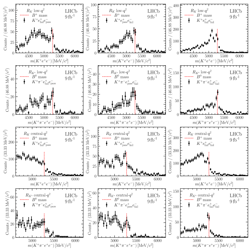
Figure 9: Invariant mass distribution of candidates in the inverted lepton identification control region. From top to bottom: $R_{K}$ $\text{low-}{q^{2}}$, $R_{K}$ $\text{central-}{q^{2}}$, $R_{{{K}^{*}}}$ $\text{low-}{q^{2}}$, $R_{{{K}^{*}}}$ $\text{central-}{q^{2}}$. (Left) candidates for which the lepton is in the control region and has the same charge as the kaon, (middle) candidates for which the lepton is in the control region and has a charge which is the opposite of that of the kaon, (right) candidates for which both leptons are in the control region.

In contrast to fully reconstructed backgrounds, backgrounds of the type ${{{B}^{+}}}\!\rightarrow{{K}^{+}}{{\pi}^{-}}({{\pi}^{0}},\gamma)X$ or ${{B}^{0}}\!\rightarrow{{K}^{*0}}{{\pi}^{-}}({{\pi}^{0}},\gamma)X$ do not have distinctive invariant-mass distributions, even with inverted PID criteria.

Figure 9 shows the invariant mass shape in the control region with inverted lepton identification criteria, as defined above. This control region contains a combination of: fully reconstructed misidentified backgrounds, singly misidentified and/or partially reconstructed backgrounds, combinatorial backgrounds, and genuine signal which passes the preselection but fails the analysis selection criteria. Calibration samples are divided into intervals of transverse momentum and pseudorapidity and used to extrapolate the yields and invariant mass shape of these components, given the full analysis selection criteria from the events in this control region. Events in the control region can contain both misidentified pions and kaons. The probability to misidentify a kaon as an electron is significantly different from the probability to misidentify a pion as an electron. Consequently the same multivariate criterion used to separate kaons and pions is used to arbitrate whether a given control region event should be treated as a pion or as a kaon when extrapolating it to the signal region. Example calibration sample maps for 2017 data and the resulting “transfer functions” that allow the control region events to be extrapolated to the fit region with nominal lepton identification criteria are shown in Fig. 10.

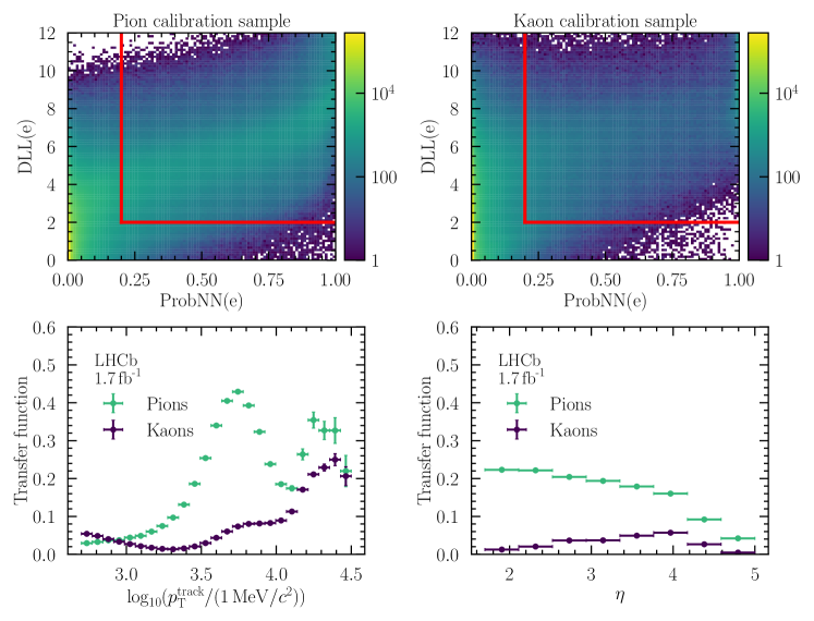
Figure 10: Upper: distributions of the PID variables in the (left) pion and (right) kaon calibration samples using 2017 data. The red lines separate control regions (left and below the line) from fit regions (right and above the line). Lower: the fraction of control region events that is expected to appear in the fit region (transfer function) as functions of track $p_{\mathrm{T}}$ and $\eta$.

The residual signal that passes the preselection but fails the analysis selection criteria is subtracted based on PID efficiencies from calibration samples and on an initial signal yield estimate from a simplified invariant mass fit. This procedure has a negligible effect on the final result. The final extrapolated misidentified backgrounds are shown in Fig. 11 for the two electron final states at $\text{low-}{q^{2}}$ and $\text{central-}{q^{2}}$. Given that the extrapolation employs data calibration samples, the depicted shapes model the ensemble effect of ${{{B}^{+}}}\!\rightarrow{{K}^{+}}{{\pi}^{-}}({{\pi}^{0}},\gamma)X$ or ${{B}^{0}}\!\rightarrow{{K}^{*0}}{{\pi}^{-}}({{\pi}^{0}},\gamma)X$ decays, without being susceptible to mismodeling of relative yields and kinematics. The narrow excesses seen between 5200 and 5300$\text{\,Me\kern-1.00006ptV\!/}c^{2}$ are attributed to the previously estimated, fully reconstructed misidentified backgrounds, and are statistically compatible with those dedicated estimates. No clear structure is seen below 5200$\text{\,Me\kern-1.00006ptV\!/}c^{2}$, however the observed shape cannot be explained by combinatorial background events alone. Although the contribution from each individual ${{{B}^{+}}}\!\rightarrow{{K}^{+}}{{\pi}^{-}}({{\pi}^{0}},\gamma)X$ or ${{B}^{0}}\!\rightarrow{{K}^{*0}}{{\pi}^{-}}({{\pi}^{0}},\gamma)X$ process is negligible, their total sum is not and needs to be accounted for in the invariant mass fit.

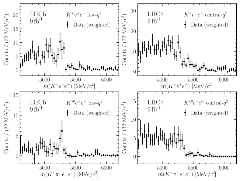
Figure 11: Distributions of misidentified background events predicted for the ${{K}^{+}}{e^{+}e^{-}}$ and ${{K}^{*0}}{e^{+}e^{-}}$ samples with full selection criteria applied.

6 Calibration of simulation and determination of efficiencies

Simulated events must be calibrated to reproduce fully all aspects of the LHC production environment and LHCb detector performance. The calibration consists of a set of weights, the product of which is applied to the simulation to ensure both reliable modeling of the different components that enter the invariant mass fits, described in the next section, and the accurate determination of detector efficiencies used to calculate $R_{K}$ and $R_{{{K}^{*}}}$. For each data-taking year the simulation is calibrated using abundant, high-purity, control samples from data. As no single data control sample can calibrate all aspects of the simulated detector performance, a multi-step sequential procedure is followed, each with its own weight, $w$, as summarized below.

1. The PID performance ($w_{\textrm{PID}}$) is calibrated as a function of track kinematics and detector occupancy using control samples of ${B}^{(+,0)}\!\rightarrow{K}^{(+,*0)}{{J\mskip-3.0mu/\mskip-2.0mu\psi}}(\!\rightarrow\ell^{+}\ell^{-})$, ${{D}^{*+}}\!\rightarrow{{D}^{0}}(\!\rightarrow{{K}^{-}}{{\pi}^{+}}){{\pi}^{+}}$, and ${{J\mskip-3.0mu/\mskip-2.0mu\psi}}\rightarrow{\mu^{+}}{\mu^{-}}$ decays;

2. The electron track reconstruction performance ($w_{\textrm{TRK}}$) is calibrated using control samples of ${B}^{(+,0)}\!\rightarrow{K}^{(+,*0)}{{J\mskip-3.0mu/\mskip-2.0mu\psi}}(\!\rightarrow{e^{+}e^{-}})$ decays. As hadron and muon efficiencies are found to agree well between data and simulation the calibration is only applied to electrons;

3. The event multiplicity and $B$ meson kinematics ($w_{\textrm{Mult\&Kin}}$) are calibrated using control samples of ${B}^{(+,0)}\!\rightarrow{K}^{(+,*0)}{{J\mskip-3.0mu/\mskip-2.0mu\psi}}(\!\rightarrow\ell^{+}\ell^{-})$ decays;

4. The L0 trigger efficiency ($w_{\textrm{L0}}$) is calibrated using control samples of ${B}^{(+,0)}\!\rightarrow{K}^{(+,*0)}{{J\mskip-3.0mu/\mskip-2.0mu\psi}}(\!\rightarrow\ell^{+}\ell^{-})$ decays;

5. An analogous procedure is followed for the HLT trigger efficiency ($w_{\textrm{HLT}}$);

6. A final set of calibrations, $w_{\textrm{Reco}}$, are computed using control samples of ${B}^{(+,0)}\!\rightarrow{K}^{(+,*0)}{{J\mskip-3.0mu/\mskip-2.0mu\psi}}(\!\rightarrow\ell^{+}\ell^{-})$ decays in order to correct residual differences in the description of reconstructed $B$ meson properties in simulation.

The full chain of calibrations is applied when computing the $q^{2}$ selection efficiency to ensure reliable modeling of the migration of events between $q^{2}$ regions. With the exception of $w_{\textrm{Mult\&Kin}}$, which uses a dedicated prior calibration chain as input, each calibration step uses as input the output of the preceding step. Calibrations are calculated separately using ${{B}^{0}}$ and ${{{B}^{+}}}$ decays and are shown to be interchangeable. As the same sample of ${B}^{(+,0)}\!\rightarrow{K}^{(+,*0)}{{J\mskip-3.0mu/\mskip-2.0mu\psi}}(\!\rightarrow\ell^{+}\ell^{-})$ decays is used to normalize decay rates in the ($R_{K}$,$R_{{{K}^{*}}}$) double ratios and to compute the calibrations, the ${B}^{0}$ calibrations are applied to $R_{K}$ and the ${{B}^{+}}$ calibrations are applied to $R_{{{K}^{*}}}$ to remove correlations arising from the statistical overlap between the normalization and calibration sample.

6.1 Particle identification

The performance of hadron and muon PID is calculated using a weight $w_{\textrm{PID}}$ computed as the efficiency with which the analysis criteria correctly identify a given particle type. These efficiencies are evaluated using a three-dimensional binning in particle momentum, particle pseudorapidity and the track multiplicity of the event, with the latter acting as a proxy for the detector occupancy. Multiplicity bins are chosen such that they are uniformly populated; the momentum and pseudorapidity binning is optimized in each bin of multiplicity. Bins are required to be sufficiently narrow to ensure that the efficiency is uniform within uncertainties across each bin, while being sufficiently broad that the statistical uncertainties are approximately Gaussian. Each dimension is therefore divided initially into equally populated bins; using an iterative procedure, adjacent bins are merged where their efficiencies differ by less than five standard deviations. For a small number of bins at the corners of the ($p$,$\eta$) phase space that remain empty, the nearest neighbor efficiency is used, while the efficiencies are rounded to 0 or 1 for those with unphysical values of efficiencies. An analogous procedure is followed to evaluate misidentification efficiencies for backgrounds.

The simulation is used to verify that the identification efficiency for a given hadron or muon is independent of PID requirements applied to other hadrons and muons in the same event. This factorization ensures that the overall efficiency is the product of the individual $w_{\textrm{PID}}$. This is not the case for electrons because their identification depends on the association of particle tracks with electromagnetic calorimeter clusters which, due to the calorimeter cell sizes, may receive contributions from more than one electron. This leads to significant correlations in their PID performance. The probability for two electrons to leave energy deposits in the same calorimeter cell strongly depends on the opening angle of the dilepton system and the momenta of the electrons, and is therefore found to be significantly higher in the $\text{central-}{q^{2}}$ signal region than in either the $\text{low-}{q^{2}}$ or the ${J\mskip-3.0mu/\mskip-2.0mu\psi}$-control region. The bias $\Delta_{\mathrm{PID}}$ is determined using simulated Run 2 ${{B}^{+}}\!\rightarrow{{K}^{+}}{{J\mskip-3.0mu/\mskip-2.0mu\psi}}(\!\rightarrow{e^{+}e^{-}})$ and ${{B}^{+}}\!\rightarrow{{K}^{+}}{e^{+}e^{-}}$ events as the relative difference between the true PID efficiency and that obtained under the assumption of full factorization. This is illustrated in Fig. 12, where $\Delta_{\mathrm{PID}}$ is shown as a function of $\mathrm{d}_{\mathrm{ECAL}}$, the distance separating two electrons at the electromagnetic calorimeter after extrapolation of their trajectories to its upstream surface.

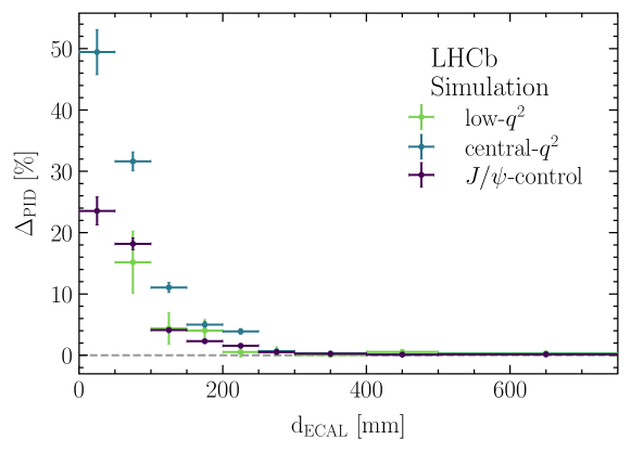
Figure 12: Factorization bias as a function of the separation between a pair of electrons in the electromagnetic calorimeter in the various $q^{2}$ regions determined using simulated $B^{+}\rightarrow K^{+}e^{+}e^{-}$ decays.

The non-factorization of electron efficiencies is sufficiently different in the signal and control regions that a dedicated treatment is required. This is most significant for those candidates having $\mathrm{d}_{\mathrm{ECAL}}<100$ mm. As only a few percent of signal candidates fall into this region they are excluded from the analysis in order to avoid having to model the effect of the overlap when computing efficiencies. Electron efficiencies are evaluated from truth-level information to account for non-factorization, but must be corrected for imperfections in modeling by simulation. Therefore, electron PID efficiencies are evaluated in both data and simulation using identically selected control samples. These efficiencies are computed in bins of $p_{\mathrm{T}}$, $\eta$, and $n_{\rm Tracks}$ and are further determined in separate categories depending on whether the electron has an associated bremsstrahlung photon or not. In each bin, $w_{\textrm{PID}}$ is defined as the ratio of the efficiency in data to that in simulation. These weights are used to correct the PID efficiency of the dielectron system determined using simulation.

The L0 calorimeter and muon triggers employ a simplified PID algorithm to select events, which can lead to biases in the measured PID performance. The calibration samples are therefore selected requiring a TIS L0 decision.

6.2 Track reconstruction

The track reconstruction performance for muons is evaluated using samples of ${{J\mskip-3.0mu/\mskip-2.0mu\psi}}\!\rightarrow{\mu^{+}\mu^{-}}$ decays detached from the PV, in which one muon is fully reconstructed in the tracking system and the presence of the other muon is inferred from activity in the muon stations and TT detector only [79]. The rate at which this second muon is also reconstructed as a track in the full detector gives the track reconstruction efficiency. The muon efficiencies are found to be described well by simulation, and no additional calibration factors are applied. Differences between data and simulation in the reconstruction performance are assumed to be the same for hadrons and muons, and to cancel in the double LU ratios.

Energy losses induced by bremsstrahlung cause a lower track reconstruction efficiency for electrons than for muons, depending on momentum and pseudorapidity. For this reason a dedicated calibration has been developed [80], which uses control samples of ${{B}^{+}}\!\rightarrow{{K}^{+}}{{J\mskip-3.0mu/\mskip-2.0mu\psi}}(\!\rightarrow{e^{+}e^{-}})$  decays in which one electron is fully reconstructed in the tracking system and the other is only reconstructed in the vertex detector. The rate at which the second electron is also reconstructed as a track in the full tracking system gives the track reconstruction efficiency. These efficiencies are evaluated in data and simulation in bins of electron momentum and pseudorapidity, as well as regions in the vertex detector which contain more or less detector material and therefore induce more or less bremsstrahlung. In each bin, $w_{\textrm{TRK}}$ is defined as the ratio of the efficiency in data to that in simulation. These are used to correct the efficiency of the dielectron system measured in simulation.

6.3 Multiplicity and kinematics

The kinematics of the $B$ hadron and the particle multiplicity of the underlying event are imperfectly simulated, partly due to limitations in how well the output of Pythia reflects $pp$ collisions at LHC energies, and partly due to limitations in the description of the LHCb detector material and the production of low-momentum particles from secondary interactions with the detector. The detector material is simulated with varying degrees of accuracy for different constituent parts of the LHCb detector, so that no single occupancy proxy can perfectly calibrate the observed event multiplicities in the detector as a whole. In common with the rest of the analysis, the calibration is performed using the track multiplicity as a proxy, and systematic uncertainties are assigned for residual imperfections in the modeling of other multiplicity observables. The kinematics are calibrated in three dimensions: the momentum, transverse momentum, and pseudorapidity of the $B$ hadron.

A dedicated boosted decision tree from the hep_ml library [81] is trained to align the simulation with data in the three kinematic observables and the occupancy proxy observable. The outputs of this decision tree are $w_{\textrm{Mult\&Kin}}$ weights which encode the relative statistical importance that the final efficiency determination should assign to each simulated event.

The calibration is performed using simulated and data samples of ${B}^{(+,0)}\!\rightarrow{K}^{(+,*0)}{{J\mskip-3.0mu/\mskip-2.0mu\psi}}(\!\rightarrow{\mu^{+}\mu^{-}})$ decays selected by the L0 muon trigger. This is both the most abundant and the highest-purity sample available; since multiplicity and kinematic corrections are by construction independent of the $B$ hadron decay it is appropriate to use the muonic decay as a proxy for the electron modes. For this independence to hold, residual data-simulation disagreements caused by PID and trigger performance must be reduced to a minimum. While data are recorded with a range of trigger configurations, only a small number of these are simulated in order to reduce the operational burden of their production and analysis. A separate correction chain of $w_{\textrm{PID}}$, $w_{\textrm{L0}}$, and $w_{\textrm{HLT}}$ is therefore computed as input to the determination of $w_{\textrm{Mult\&Kin}}$, using only data taken with the simulated trigger configurations.

6.4 Trigger

The L0 TOS efficiencies are calibrated as a function of muon transverse momentum and electron transverse energy, with the electron efficiency calibrated separately for each of the three electromagnetic calorimeter regions. The efficiency denominator is the number of TIS events, while the numerator is the number of TIS events which are also TOS on the lepton trigger of interest [82]. In order to minimize non-factorizable effects, the muon efficiency is computed with hadron or electron TIS events as the denominator, while the electron efficiency is computed with hadron or muon TIS events as the denominator. Alternative definitions of the denominator are used as cross-checks and give compatible results. Efficiencies are calculated on data and simulation, and the $w_{\textrm{L0}}$ weights encode the ratio of data and simulation efficiencies in each kinematic bin. Since there are two leptons in each event, the final per-event weight has to be corrected in order not to count twice events in which both leptons satisfy the TOS criteria, where

$$w_{\textrm{L0}}^{\textrm{TOS}}=\frac{\varepsilon_{\textrm{TOS}}^{\text{data}}}{\varepsilon_{\textrm{TOS}}^{\text{MC}}}=\frac{1-\left(1-\varepsilon_{\text{{TOS}}}^{\text{data}}({\ell^{+}})\right)\cdot\left(1-\varepsilon_{\text{{TOS}}}^{\text{data}}({\ell^{-}})\right)}{1-\left(1-\varepsilon_{\text{{TOS}}}^{\text{MC}}({\ell^{+}})\right)\cdot\left(1-\varepsilon_{\text{{TOS}}}^{\text{MC}}({\ell^{-}})\right)}\,.$$ (4)

The L0 TIS efficiencies are calibrated as a function of the $B$ hadron transverse momentum and the event track multiplicity, since the TIS trigger is by definition more likely to select events with higher activity in the detector. The efficiency denominator is the number of lepton and hadron TOS events, to maximize the available control sample yields. The efficiency numerator is the number of those events which are also TIS. As with the TOS weights, the efficiencies are calculated on data and simulation, and the $w_{\textrm{L0}}$ weights encode the ratio of data and simulation efficiencies in each kinematic bin.

The HLT efficiencies are calibrated analogously to the L0 efficiencies, as a function of the event track multiplicity. The same control samples are used, with separate $w_{\textrm{HLT}}$ calibrations for the L0 TIS and TOS categories. The efficiencies are calculated on data and simulation, and the $w_{\textrm{HLT}}$ weights are defined as the ratio of data and simulation efficiencies in each bin.

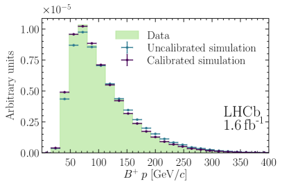
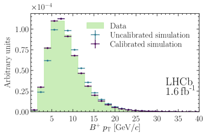
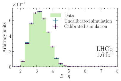
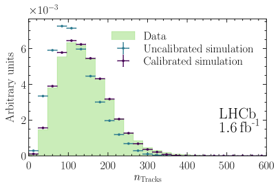
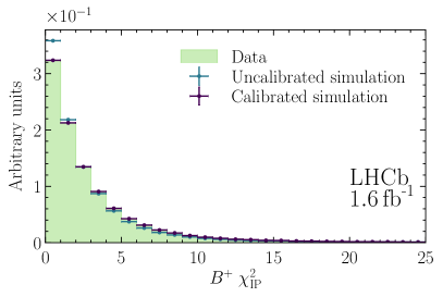
Figure 13: Distributions of selected measured quantities for TOS ${{B}^{+}}\!\rightarrow{{K}^{+}}{{J\mskip-3.0mu/\mskip-2.0mu\psi}}({e^{+}e^{-}})$ candidates in the 2016 data, compared with simulation before (red) and after (blue) calibrations.

6.5 Candidate reconstruction

Residual discrepancies between data and simulation arise from differences in the performance of the reconstruction, particularly in the uncertainties assigned to track trajectories that in turn affect derived quantities such as the vertex fit quality. A second boosted decision tree, trained analogously to $w_{\textrm{Mult\&Kin}}$, is used to improve further the data-simulation agreement. As reconstruction differences are sensitive to the particle species being calibrated, their calibration is performed separately for the electron and muon final states, and separately for each L0 trigger category. The reweighting is performed as a function of five variables: the same three kinematic quantities used for $w_{\textrm{Mult\&Kin}}$ as well as the $\chi^{2}_{\text{IP}}$ of the $B$ and ${J\mskip-3.0mu/\mskip-2.0mu\psi}$ mesons, where $\chi^{2}_{\text{IP}}$ for a given particle is defined as the difference in the $\chi^{2}$ of the PV fit with and without that particle. Examples of the final agreement between data and simulation are presented in Fig. 13.

6.6 Migration in $q^{2}$

As a result of these calibrations the simulation accurately models most features of the data. However, the migration of electron candidates across the $q^{2}$ spectrum is sensitive to residual misalignments between data and simulation that affect the $q^{2}$ resolution and its behavior in the tails; particular attention is required when evaluating the impact of bremsstrahlung. The $q^{2}$ of simulated candidates is therefore smeared using a function with parameters determined by fitting the dielectron mass spectra from ${B}^{(+,0)}\!\rightarrow{K}^{(+,*0)}{{J\mskip-3.0mu/\mskip-2.0mu\psi}}(\!\rightarrow{e^{+}e^{-}})$ decays in data and simulation. The smeared dilepton mass for each candidate in simulation is given by

$$m^{\mathrm{Res}}=m^{\mathrm{true}}+s_{\sigma}\cdot(m^{\mathrm{reco}}-m^{\mathrm{true}})+\Delta\mu+(1-s_{\sigma})\cdot(\mu^{\mathrm{MC}}-M_{{{J\mskip-3.0mu/\mskip-2.0mu\psi}}}^{\mathrm{PDG}}),$$ (5)

where $m^{\mathrm{true}}$ is the generated dilepton mass calculated using the difference between the generated kinematics of the parent $B$ hadron and of the $K^{(+,*0)}$; $m^{\mathrm{reco}}$ is the reconstructed dilepton mass in simulation; $s_{\sigma}$ is the ratio of the widths of the reconstructed mass distributions in data and simulation; $\Delta\mu$ is the difference in the means of the reconstructed mass distributions in data and simulation; $\mu^{\mathrm{MC}}$ is the mean mass determined from a fit to simulated data.

Unbinned maximum-likelihood fits are performed separately for the ${{B}^{+}}$ and ${B}^{0}$ modes in each trigger and bremsstrahlung category and for each data-taking year. The full selection is applied leading to excellent sample purity. A modified Crystal Ball function [83] with power law tails both above and below the mean mass value (DSCB) is used to model the dielectron spectrum, with the remaining combinatorial background modeled using an exponential function. The high quality of the fit is illustrated by comparing 2018 data and simulation in Fig. 14. The smeared mass allows the efficiency measured in a given range of reconstructed $q^{2}$ to be transformed into the corresponding range of true $q^{2}$, defined before emission of final state photon radiation, as required for the measurement of the lepton universality ratios. This correction is denoted as $w_{\textrm{Res}}$.

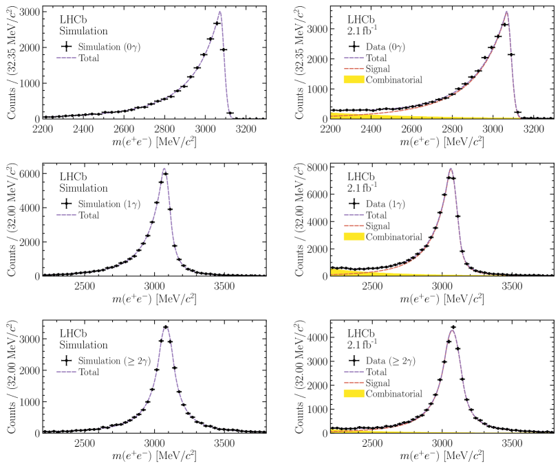
Figure 14: Distributions of the dielectron invariant mass for ${{B}^{+}}\!\rightarrow{{K}^{+}}{{J\mskip-3.0mu/\mskip-2.0mu\psi}}({e^{+}e^{-}})$ candidates in (left) simulation and (right) data, for each of the three bremsstrahlung categories (from top to bottom), overlaid with the projections of the fit model. The candidates correspond to the 2018 data and the TIS trigger category.

6.7 Determination of efficiencies

The overall efficiency for the signal and resonant control modes is determined using fully calibrated simulation samples for each data-taking year and trigger category. Efficiencies for background samples that are modeled in the invariant mass fit are determined in the same way. To make the best use of computing resources, only events in which all of the decay products of a $B$ candidate are generated within the geometric acceptance of the LHCb detector are processed by the detector simulation. The efficiency, $\varepsilon_{\textrm{geo}}$, of this generator selection is evaluated for each signal mode as a function of $q^{2}$ using dedicated samples generated without LHCb detector acceptance requirements. The overall efficiency is then given by

$$\varepsilon_{\textrm{tot}}=\varepsilon_{\textrm{geo}}\times(\varepsilon_{\mathrm{MVA}}\times\varepsilon_{\mathrm{Presel}}\times\varepsilon_{\mathrm{Trg}}\times\varepsilon_{\mathrm{PID}}|\mathrm{geo}),$$ (6)

where $\varepsilon_{\mathrm{MVA}}$ is the efficiency of the multivariate selection, $\varepsilon_{\mathrm{Presel}}$ is the efficiency of the preselection excluding PID criteria, $\varepsilon_{\mathrm{Trg}}$ is the trigger efficiency, and $\varepsilon_{\mathrm{PID}}$ is the PID efficiency.

The strategy of applying ${B}^{0}$ calibrations to ${{B}^{+}}$ final states and vice versa reduces correlations in the total efficiency determination but can not eliminate them entirely. The most significant irreducible correlation is caused by the fact that the same simulated samples are used to compute both the resonant mode efficiencies and the data-simulation calibrations.

Further residual correlations occur because of calibrations that are shared between the muon and electron final states, because the TIS and TOS samples used in the calibrations are not required to be mutually exclusive in order to increase the control sample sizes, and because the resonant control modes are used to compute the trigger efficiencies and train the algorithms that produce the $w_{\textrm{Mult\&Kin}}$ and $w_{\textrm{Reco}}$ weights. These correlations are evaluated using a bootstrapping procedure as follows. Each reconstructed data or simulation candidate is assigned one hundred different Poisson-distributed weights with a mean value of 1. The generation of weights is performed using a common seed for each event based on a unique event identifier. This allows 100 different correction maps to be generated and their correlations assessed by comparing the simulation efficiencies and data sample yields for each bootstrapped data sample. The distributions of the bootstrapped efficiencies are verified to be well described by Gaussian functions. The relative efficiencies of nonresonant and resonant modes in both low- and $\text{central-}{q^{2}}$ are found to vary between 0.7 and 0.9 for both electron and muon modes.

7 Simultaneous invariant mass fit

The signal and resonant control mode yields in Eqs. 2–3, as well as those of the $\psi{(2S)}$ equivalents, are obtained using simultaneous maximum-likelihood fits to the invariant mass distributions of selected $B$ meson candidates. The invariant mass is calculated using the decay tree fitter algorithm to constrain the momentum vector of the $B$ meson to be aligned with its displacement vector. The fits to the signal modes are unbinned, whereas the fits to the more abundant resonant modes are performed to data that are binned in the invariant mass. The fits are based on the RooFit [84] and Root [85] frameworks, with a custom implementation of the probability density functions (PDFs) [86] that eliminates biases in binned fits caused by sharp PDF variations within a given bin. Events selected in the TIS and TOS trigger categories are fit simultaneously. The structure allows the fit to be performed either for the signal mode yields; for the resonant mode yields; simultaneously for the signal and resonant mode yields; or simultaneously for $R_{K}$ and $R_{{{K}^{*}}}$ by using the efficiencies, determined on calibrated simulation samples, and the covariance matrix, obtained by bootstrapping the efficiencies, as constraints in the invariant mass fit.

Similarly, the fit can be executed for each of the Run 1, Run 2p1, or Run 2p2 data-taking periods, or for all three simultaneously. The configuration in which $R_{K}$ and $R_{{{K}^{*}}}$ are fitted simultaneously in all trigger categories and data-taking periods is referred to as “nominal” and used to produce the results reported in Sec. 10. All constraints described are implemented as Gaussian functions with mean and width corresponding to the central value and the uncertainty associated with the parameter being constrained. Systematic uncertainties and their correlations are instead accounted for including a multiplicative factor to the $R_{K}$ and $R_{{{K}^{*}}}$ values in each fit projection category, which is constrained using a Gaussian function with mean of unity and a width representing the relative uncertainty of the relevant source. Multidimensional Gaussian constraints are implemented for correlated parameters.

Table 5: Invariant mass ranges used in the fits. The fit type indicates where the dilepton invariant mass is constrained to the known ${J\mskip-3.0mu/\mskip-2.0mu\psi}$ ($\psi{(2S)}$) mass.

Lepton	$q^{2}$ region	Fit type	Range ($\text{\,Me\kern-1.00006ptV\!/}c^{2}$)
Electron	low, central	unconstrained	4600–6200
	${J\mskip-3.0mu/\mskip-2.0mu\psi}$	unconstrained	4600–6200
		constrained	4900–6200
	$\psi{(2S)}$	constrained	5100–5750
Muon	low, central	unconstrained	5150–5850
	${J\mskip-3.0mu/\mskip-2.0mu\psi}$	unconstrained	5100–6100
		constrained	5100–6100
	$\psi{(2S)}$	constrained	5100–5750

Table 6: Observed yields of the six signal and control modes and their statistical uncertainties.

LU observable	Muon ($\times 10^{3})$	Electron ($\times 10^{3})$
low-$q^{2}$ $R_{K}$	$\left(4\right.$$1.25\pm 0.04$$\left.2\right)\times 10^{3}$	$\left(\right.$$0.305\pm 0.024$$\left.\right)\times 10^{3}$
low-$q^{2}$ $R_{{{K}^{*}}}$	$\left(4\right.$$1.001\pm 0.034$$\left.2\right)\times 10^{3}$	$\left(\right.$$0.247\pm 0.022$$\left.\right)\times 10^{3}$
central-$q^{2}$ $R_{K}$	$\left(4\right.$$4.69\pm 0.08$$\left.2\right)\times 10^{3}$	$\left(9\right.$$1.19\pm 0.05$$\left.5\right)\times 10^{3}$
central-$q^{2}$ $R_{{{K}^{*}}}$	$\left(4\right.$$1.74\pm 0.05$$\left.2\right)\times 10^{3}$	$\left(\right.$$0.443\pm 0.028$$\left.\right)\times 10^{3}$
${J\mskip-3.0mu/\mskip-2.0mu\psi}$ $R_{K}$	$\left(2.964\pm 0.002\right)\times 10^{3}$	$\left(7.189\pm 0.015\right)\times 10^{2}$
${J\mskip-3.0mu/\mskip-2.0mu\psi}$ $R_{{{K}^{*}}}$	$\left(9.733\pm 0.010\right)\times 10^{2}$	$\left(2.517\pm 0.009\right)\times 10^{2}$

The invariant mass resolution of the resonant control modes can be improved by constraining the dilepton invariant mass to be equal to that of the ${J\mskip-3.0mu/\mskip-2.0mu\psi}$ or $\psi{(2S)}$ resonance, and this improvement is particularly large for electrons because of their poorer intrinsic resolution. The unconstrained dilepton invariant mass is used in the nominal fits in order to match the modeling of the nonresonant mode and reduce systematic uncertainties in the double ratio, whereas the constrained mass is used for cross-checks and systematic studies. The fit ranges used in the analysis are given in Table 5; where studies of specific systematic uncertainties use different fit ranges, these are noted in Section 9.

Large ensembles of pseudodata generated with the component yields observed in data are used to validate that the fit is unbiased and gives accurate uncertainties. The uncertainties on the $R_{K}$ and $R_{{{K}^{*}}}$ double ratios are found to be asymmetric, which is accounted for when reporting the results in Sec. 10. The result of the nominal simultaneous fit to the signal and ${J\mskip-3.0mu/\mskip-2.0mu\psi}$ modes is shown in Fig. 15 for the muon and Fig. 16 for the electron final states. The observed yields of the six signal and control modes, as well as their statistical uncertainties, are reported in Table 6.

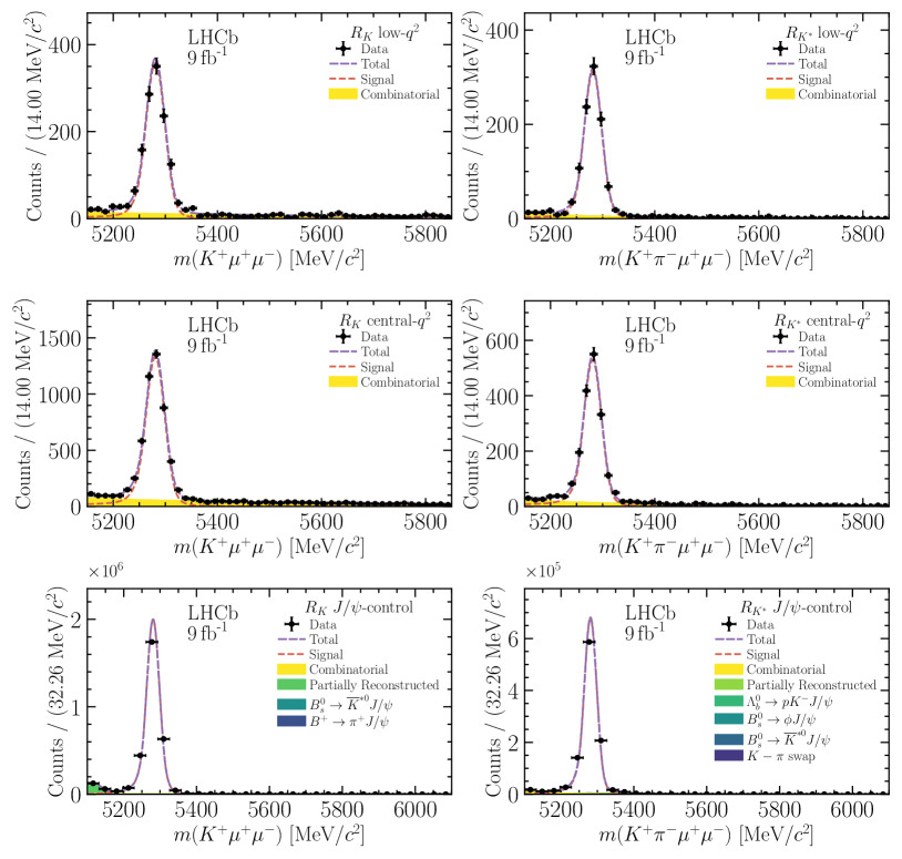
Figure 15: Distributions of (left) $m(K^{+}\mu^{+}\mu^{-})$ and (right) $m(K^{+}\pi^{-}\mu^{+}\mu^{-})$ of $\text{low-}{q^{2}}$, $\text{central-}{q^{2}}$, and ${J\mskip-3.0mu/\mskip-2.0mu\psi}$-control regions (from top to bottom), overlaid with the projections of the fit model. Each of the fit components are discussed in Section 7.1.

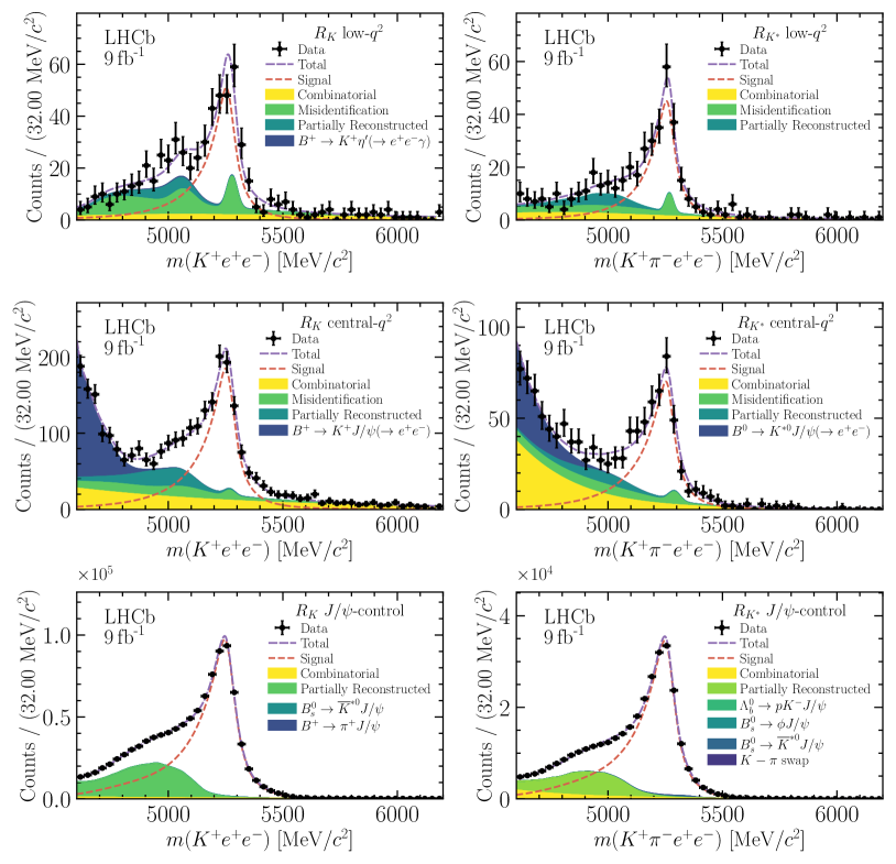
Figure 16: Distributions of (left) $m(K^{+}e^{+}e^{-})$ and (right) $m(K^{+}\pi^{-}e^{+}e^{-})$ in the (top to bottom) $\text{low-}{q^{2}}$, $\text{central-}{q^{2}}$, and ${J\mskip-3.0mu/\mskip-2.0mu\psi}$-control regions, overlaid with the projections of the fit model. Each of the fit components are discussed in Sec. 7.1.

7.1 Fit components

7.1.1 Signal and control modes

For fits where the dilepton invariant mass is unconstrained, the signal and resonant control mode PDFs are obtained by fitting analytic functions to fully calibrated simulated samples in each data-taking period and trigger category. The best-fit values of the function parameters are subsequently fixed in nominal fits to data and varied in pseudoexperiments to estimate the associated systematic uncertainties, which are found to be negligible. For the final states with electrons, individual PDFs are obtained by fitting simulated samples separated according to their bremsstrahlung category; these are subsequently added in proportion to the abundance of bremsstrahlung categories observed in fully calibrated simulation samples to obtain an overall PDF for use in data fits. The relative abundance of the bremsstrahlung categories with zero, one, and two or more reconstructed bremsstrahlung photons corresponds to $25\%$, $50\%$, and $25\%$, respectively. A systematic uncertainty is assigned to account for the finite knowledge of these fractions. Fits constraining the ${J\mskip-3.0mu/\mskip-2.0mu\psi}$ mass are only used for cross-checks and systematic uncertainties and have a better mass resolution which does not depend significantly on the dielectron bremsstrahlung category. For this reason the data fit PDFs are obtained in a simplified way in this case by fitting analytical functions to uncalibrated simulation samples without any separation for the bremsstrahlung category.

The analytical functions used to define the signal and resonant control mode PDFs are listed in Table 7. The overall PDF normalizations vary freely for each data-taking period and trigger category. The different treatment of the electron signal and ${J\mskip-3.0mu/\mskip-2.0mu\psi}$ PDFs obtained without a constraint on the dielectron invariant mass is motivated by a combination of two effects. First, the ${J\mskip-3.0mu/\mskip-2.0mu\psi}$-$q^{2}$ range is significantly narrower above the mean ${J\mskip-3.0mu/\mskip-2.0mu\psi}$ meson mass than below it, which deforms the right-hand tail of the PDF. Second, the veto on cascade $B\!\rightarrow{\psi{(2S)}}(\rightarrow{{J\mskip-3.0mu/\mskip-2.0mu\psi}}X)K^{(*)}$ decays deforms the left-hand tail of the PDF. An acceptable fit quality can therefore only be obtained by adding either one or two Gaussian functions, depending on the bremsstrahlung category, to the PDF. The normalization of these Gaussian functions relative to the principal DSCB component is a free parameter of the fit to data and simulation.

Residual differences between data and simulation are parametrized through a shift in the mean value of the signal PDF and a scale factor applied to the width of this PDF. These parameters are independent for muons and electrons, and independent for each data-taking period and trigger category, but shared between the signal and control modes. Prior to calibrating the simulation the scale factors are typically between 1.1 and 1.15, while the mean value of the PDF is shifted by ${\mathcal{O}}(10\text{\,Me\kern-1.00006ptV\!/}c^{2})$. After the simulation is calibrated, the scale factors are found to be compatible with unity while the mean value shifts are reduced to ${\mathcal{O}}(1\text{\,Me\kern-1.00006ptV\!/}c^{2})$. The scale factors and mean values are left as free parameters within the nominal fit to account for systematic uncertainties caused by residual imperfections in the calibration of simulation.

Table 7: Analytical functions used to describe the signal and resonant control modes. The fit type refers to whether the dilepton invariant mass is constrained to that of the ${J\mskip-3.0mu/\mskip-2.0mu\psi}$ ($\psi{(2S)}$) resonance or not. Category refers to the bremsstrahlung category in the case of electron modes. Hypatia refers to a two-sided version of a generalized Crystal Ball distribution introduced in Ref. [87].

Lepton	$q^{2}$ Region	Fit type	Category	Function
Electron	low, central	unconstrained	$\geq$2all	DSCB
	${J\mskip-3.0mu/\mskip-2.0mu\psi}$ $(2)$	unconstrained	$\geq$all0	DSCB + Gaussian
			$\geq$all1	DSCB + two Gaussians
			$\phantom{al}\geq$2	DSCB + two Gaussians
		unconstrained	$\geq$2all	DSCB
	$\psi{(2S)}$	unconstrained	$\geq$2all	DSCB
Muon	low, central	unconstrained		DSCB + two Gaussians
	${J\mskip-3.0mu/\mskip-2.0mu\psi}$ $(2)$	unconstrained		DSCB + two Gaussians
		unconstrained		Hypatia + Gaussian
	$\psi{(2S)}$	unconstrained		Hypatia + Gaussian

7.1.2 Combinatorial background

The combinatorial background is described by a single exponential function for the resonant modes and the nonresonant muon modes. For the nonresonant electron modes, the multivariate selections and the $m_{\mathrm{corr}}$ criteria are found to induce a deviation from an exponential shape by introducing a sculpting of the invariant mass spectrum within the fit ranges considered. Same-sign lepton data are exploited to calibrate the modeling of the combinatorial shape in the low- and $\text{central-}{q^{2}}$ bins for each data-taking period and trigger category. The sculpting is described by a factor $1/\bigl{(}1+\exp(s(m-m_{0})\bigr{)}$ that multiplies the exponential function and where the parameters ($s,m_{0}$) are obtained from fits to same-sign data and fixed in fits to the nonresonant electron signal modes. Systematic uncertainties associated with the procedure are evaluated by varying $(s,m_{0})$ according to the uncertainty determined in same-sign data fits. The slope of the exponential function is left as a free parameter in the fit. The PDF normalization is allowed to vary independently for each data-taking period and trigger category in all cases.

7.1.3 ${J\mskip-3.0mu/\mskip-2.0mu\psi}$ leakage in the central-$q^{2}$ region

A significant fraction of ${J\mskip-3.0mu/\mskip-2.0mu\psi}$ decays which leak into the central $q^{2}$ region also fall within the invariant mass fit range for the electron mode. The energy loss which causes their invariant dielectron mass to fall within the central $q^{2}$ region also causes their invariant $B$ meson mass to be shifted to values much lower than the signal. The extended fit range in signal electron modes, down to 4600 $\text{\,Me\kern-1.00006ptV\!/}c^{2}$, allows the interplay between this background component, the combinatorial background, and specific physics backgrounds to be well modeled. The ${J\mskip-3.0mu/\mskip-2.0mu\psi}$ leakage PDFs are described using unbinned templates derived from fully calibrated simulation samples. The normalization of the PDF is also obtained from fully calibrated simulation samples for each data-taking period and trigger category. It is constrained in fits to data, with a $20\%$ uncertainty which reflects not only the measured uncertainties on simulation but also accounts for any residual disagreement between the data and simulation.

7.1.4 Specific backgrounds at low- and central-$q^{2}$

No significant specific backgrounds are present in the low- and $\text{central-}{q^{2}}$ muon modes.

For the electron case, the remaining specific backgrounds are $B^{+,0}\!\rightarrow({{K}^{+}}{{\pi}^{-}}\pi^{+,0}){e^{+}e^{-}}$ in the case of the ${B}^{0}$ mode, $B^{+,0}\!\rightarrow({{K}^{+}}\pi^{0,-}){e^{+}e^{-}}$ in the case of the ${{B}^{+}}$ mode, and misidentified backgrounds for both modes. At low-$q^{2}$, there is an additional small contribution to the ${{B}^{+}}$ mode from $B^{+}\!\rightarrow K^{+}\eta^{\prime}(\!\rightarrow{e^{+}e^{-}}\gamma)$ decays which is included in the fit model with a shape determined from simulation generated accounting for the $\eta^{\prime}(\!\rightarrow{e^{+}e^{-}}\gamma)$ dynamics [88] and constrained to its expectation [89].

The ${B}^{0}$ mode backgrounds that are not affected by misidentification are described using unbinned templates obtained from fully calibrated simulation of ${{{B}^{+}}}\!\rightarrow{{K}^{+}}{{\pi}^{-}}{{\pi}^{+}}{e^{+}}{e^{-}}$ decays. Their normalization is allowed to vary freely for each data-taking period and trigger category in all cases.

The ${{B}^{+}}$ mode backgrounds that are not affected by misidentification are also described using unbinned templates obtained from fully calibrated simulation samples. As the ${{B}^{+}}$ mode backgrounds include the ${{B}^{0}}\!\rightarrow K^{*0}{e^{+}e^{-}}$ signal, it is desirable to constrain their normalization using the ${B}^{0}$ mode in the simultaneous fit. This both improves sensitivity and, more importantly, enforces that the two measurements of LU are coherent: one is measured at the best-fit point of the other. To enable this, individual components of the $B^{+,0}\!\rightarrow({{K}^{+}}\pi^{0,-}){e^{+}e^{-}}$ background are considered separately, with their normalizations constrained relative to that of the ${{B}^{0}}\!\rightarrow K^{*0}{e^{+}e^{-}}$ signal as explained below. The specific contributions identified are:

1. ${{B}^{0}}\!\rightarrow({{K}^{+}}{{\pi}^{-}}){e^{+}e^{-}}$ where the ${K}^{+}$ ${\pi}^{-}$ invariant mass is within 100$\text{\,Me\kern-1.00006ptV\!/}c^{2}$ of the ${K}^{*0}$ invariant mass: these correspond directly to the ${B}^{0}$ mode signal and their normalization is constrained from its normalization corrected by the relative efficiencies obtained from fully calibrated simulation.

2. ${{B}^{0}}\!\rightarrow({{K}^{+}}{{\pi}^{-}}){e^{+}e^{-}}$ where the ${K}^{+}$ ${\pi}^{-}$ invariant mass is more than 100$\text{\,Me\kern-1.00006ptV\!/}c^{2}$ from the ${K}^{*0}$ invariant mass, and the ${K}^{+}$ ${\pi}^{-}$ pair originates from the ${K}^{*0}$ resonance: these correspond to the tail of the Breit-Wigner distribution describing the ${K}^{*0}$ resonance. Their normalization is also constrained from the ${B}^{0}$ mode signal normalization corrected by the relative efficiencies obtained from fully calibrated simulation samples and by the relative efficiency of the 100$\text{\,Me\kern-1.00006ptV\!/}c^{2}$ mass window applied to the ${K}^{*0}$ Breit-Wigner distribution.

3. ${{B}^{0}}\!\rightarrow({{K}^{+}}{{\pi}^{-}}){e^{+}e^{-}}$ where the ${K}^{+}$ ${\pi}^{-}$ invariant mass is less than 1200$\text{\,Me\kern-1.00006ptV\!/}c^{2}$ and the ${K}^{+}$ ${\pi}^{-}$ pair does not originate from the ${K}^{*0}$ resonance: these correspond to the non-resonant (S-wave) ${{B}^{0}}\!\rightarrow({{K}^{+}}{{\pi}^{-}}){e^{+}e^{-}}$ counterpart of the ${B}^{0}$ mode signal. Their relative decay rate has been directly measured in Ref. [54] for muonic modes and that measurement, together with relative efficiencies obtained from fully calibrated simulation samples, is used to constrain the normalization of this background component.

4. ${{B}^{0}}\!\rightarrow({{K}^{+}}{{\pi}^{-}}){e^{+}e^{-}}$ where the ${K}^{+}$ ${\pi}^{-}$ invariant mass is greater than 1200$\text{\,Me\kern-1.00006ptV\!/}c^{2}$ and the ${K}^{+}$ ${\pi}^{-}$ pair does not originate from the ${K}^{*0}$ resonance: these include S-wave counterparts of the signal, for which the decay rate is estimated in two different ways: extrapolating linearly the known branching ratios for $m({{K}^{+}}{{\pi}^{-}})$ below 1200$\text{\,Me\kern-1.00006ptV\!/}c^{2}$ up to 2400$\text{\,Me\kern-1.00006ptV\!/}c^{2}$ into four regions of $m({{K}^{+}}{{\pi}^{-}})$, and using the full amplitude model of ${K}^{+}$ ${\pi}^{-}$ ${J\mskip-3.0mu/\mskip-2.0mu\psi}$ decays developed in Ref. [90]. These estimates are found to be compatible, and the linear extrapolation, together with relative efficiencies obtained from fully calibrated simulation samples, is used to constrain the normalization of this background component. A 50% relative systematic uncertainty is assigned to this extrapolation.

5. ${{{B}^{+}}}\!\rightarrow({{K}^{+}}{{\pi}^{0}}){e^{+}e^{-}}$: this is the isospin partner of the neutral signal decay, with analogous resonant and non-resonant $K\pi$ components. The normalization of its components is constrained to that of the analogous $({{K}^{+}}{{\pi}^{-}})$ components, corrected by relative efficiencies obtained from fully calibrated simulation, and scaled by an isospin extrapolation factor which accounts for differences in the ${{B}^{+}}$ and ${B}^{0}$ lifetimes as well as ${{K}^{*0}}\!\rightarrow{{K}^{+}}{{\pi}^{-}}$ and ${{K}^{*+}}\!\rightarrow{{K}^{+}}{{\pi}^{0}}$ relative decay rates. A relative systematic uncertainty of 10% is assigned to the isospin extrapolation factor.

Misidentified backgrounds are described using shapes constructed from the histograms in Fig. 11 in Sec. 5.3. The baseline approach models these backgrounds with a Gaussian component for the fully reconstructed doubly misidentified backgrounds that peak between 5200 and 5300$\text{\,Me\kern-1.00006ptV\!/}c^{2}$, a second empirical Gaussian component to describe the non-combinatorial backgrounds below 5200$\text{\,Me\kern-1.00006ptV\!/}c^{2}$, and an exponential component sculpted in the same way described in Sec. 7.1.2. Due to similar and compatible misidentification rates and data-taking conditions between Run 2p1 and Run 2p2, the determination of the misidentified background component model is obtained combining the predicted background events in these periods. The resulting nominal misidentified background components are shown in Fig. 17. An alternative approach based on kernel density estimates is used to assign a systematic uncertainty to the choice of model.

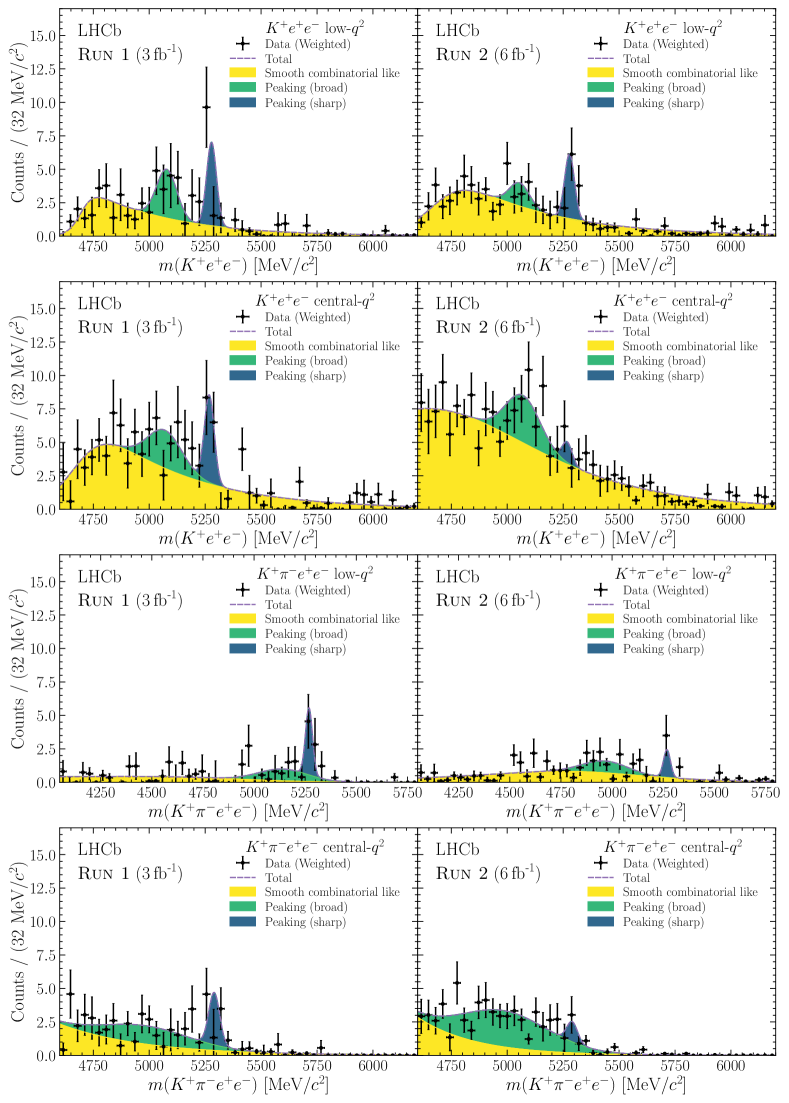
Figure 17: Template shapes for misidentified backgrounds obtained from data. The shapes for Run 1 are given on the left, the shapes for Run 2 are given on the right. From top to bottom, the shapes for $R_{K}$ in $\text{low-}{q^{2}}$, $R_{K}$ in $\text{central-}{q^{2}}$, $R_{{{K}^{*}}}$ in $\text{low-}{q^{2}}$ and $R_{{{K}^{*}}}$ in $\text{central-}{q^{2}}$ regions are given.

The yields of these backgrounds in the nominal fit are constrained using the sum of the weighted entries in the histograms and the associated uncertainty. The lepton identification requirements used to define the control region dataset, as well as the threshold used to assign an event as pion- or kaon-like, are varied to compute systematic uncertainties.

7.1.5 Specific backgrounds in ${{B}^{+}}$ resonant modes

Specific backgrounds in ${{B}^{+}}$ resonant modes are listed in Table 1. The ${{B}^{+}}\!\rightarrow{{\pi}^{+}}{{J\mskip-3.0mu/\mskip-2.0mu\psi}}(\!\rightarrow{\ell^{+}}{\ell^{-}})$ background is modeled using a DSCB function for which the parameters are obtained from uncalibrated simulation samples. The ${{B}^{0}_{s}}\!\rightarrow{{\kern 1.79993pt\overline{\kern-1.79993ptK}}{}^{*0}}{{J\mskip-3.0mu/\mskip-2.0mu\psi}}(\!\rightarrow{\ell^{+}}{\ell^{-}})$ background is described using an unbinned template obtained from simulation samples.

Backgrounds from ${B}\!\rightarrow X{{J\mskip-3.0mu/\mskip-2.0mu\psi}}(\!\rightarrow{\mu^{+}\mu^{-}})$ and ${B}\!\rightarrow X{\psi{(2S)}}(\!\rightarrow{\mu^{+}\mu^{-}})$ decays are modeled using unbinned templates obtained from fully calibrated simulation samples. Inclusive simulated samples of ${B}^{0}_{s}$, ${{B}^{+}}$, and ${B}^{0}$ decays are used to construct the templates. The relative normalization of these background samples is fixed to the known relative production fractions and decay rates, while their overall normalization freely varies in the fit. An analogous procedure is followed in the case of ${B}\!\rightarrow X{{J\mskip-3.0mu/\mskip-2.0mu\psi}}(\!\rightarrow{e^{+}e^{-}})$ and ${B}\!\rightarrow X{\psi{(2S)}}(\!\rightarrow{e^{+}e^{-}})$, with adjustments for the significantly wider mass range used in the unconstrained ${J\mskip-3.0mu/\mskip-2.0mu\psi}$ electron fits.

The $\psi{(2S)}$ electron mode fits require two additional backgrounds to be modeled: the leakage of ${{B}^{+}}\!\rightarrow{{K}^{+}}{{J\mskip-3.0mu/\mskip-2.0mu\psi}}$ decays into the $\psi{(2S)}$ $q^{2}$ range, and partially reconstructed ${{B}^{+}}\!\rightarrow{{K}^{+}}{\psi{(2S)}}(\rightarrow{{J\mskip-3.0mu/\mskip-2.0mu\psi}}(\!\rightarrow{e^{+}e^{-}})X)$ decays. Both are modeled using unbinned templates obtained from fully calibrated simulation samples, and their normalizations are allowed to vary freely in the fit.

7.1.6 Specific backgrounds in ${B}^{0}$ resonant modes

Specific backgrounds in ${B}^{0}$ resonant modes are listed in Table 2. Backgrounds from ${\mathchar 28931\relax}^{0}_{b}$ processes are corrected for the known inaccuracies in the Pythia modeling of ${\mathchar 28931\relax}^{0}_{b}$ kinematics using the same correction factors as in Ref. [22]. Corrections are applied as a two-dimensional function of the ${\mathchar 28931\relax}^{0}_{b}$ transverse momentum and pseudorapidity, separately for samples simulated at center-of-mass energies of 7, 8, and 13 TeV. The ${B}\!\rightarrow X{{J\mskip-3.0mu/\mskip-2.0mu\psi}}(\!\rightarrow{\mu^{+}\mu^{-}})$ and ${B}\!\rightarrow X{\psi{(2S)}}(\!\rightarrow{\mu^{+}\mu^{-}})$ backgrounds are modeled analogously to the procedure followed in the ${{B}^{+}}$ resonant modes. Similarly, the ${{B}^{0}}\!\rightarrow{{K}^{*0}}{{J\mskip-3.0mu/\mskip-2.0mu\psi}}$ leakage in the $\psi{(2S)}$ electron fits and the background from partially reconstructed ${{B}^{0}}\!\rightarrow{{K}^{*0}}{\psi{(2S)}}(\rightarrow{{J\mskip-3.0mu/\mskip-2.0mu\psi}}({e^{+}e^{-}})X)$ decays are modeled analogously to the procedure followed in the ${{B}^{+}}$ resonant modes.

The ${{\mathchar 28931\relax}^{0}_{b}}\!\rightarrow p{{K}^{-}}{{J\mskip-3.0mu/\mskip-2.0mu\psi}}(\!\rightarrow{\ell^{+}}{\ell^{-}})$ background is described using unbinned templates obtained from fully calibrated simulation samples. In addition to the correction of the ${\mathchar 28931\relax}^{0}_{b}$ kinematics, the ${{\mathchar 28931\relax}^{0}_{b}}\!\rightarrow p{{K}^{-}}{{J\mskip-3.0mu/\mskip-2.0mu\psi}}(\!\rightarrow{\ell^{+}}{\ell^{-}})$ simulated samples are also corrected for the amplitude structure of the ${\mathchar 28931\relax}^{0}_{b}$ decay measured in Ref. [91]. The relative normalization is constrained from its known decay rate [92], the measured ${\mathchar 28931\relax}^{0}_{b}$ production fraction [93, 94], and the selection efficiency measured using fully calibrated simulation samples. The same strategy is used for both muon and electron modes.

The ${{B}^{0}_{s}}\!\rightarrow{{\kern 1.79993pt\overline{\kern-1.79993ptK}}{}^{*0}}{{J\mskip-3.0mu/\mskip-2.0mu\psi}}(\!\rightarrow{\ell^{+}}{\ell^{-}})$ background is described using the same PDF as the ${J\mskip-3.0mu/\mskip-2.0mu\psi}$ control mode, shifted to account for the known difference in ${B}^{0}_{s}$ and ${B}^{0}$ masses. The normalization of this background is allowed to vary freely in the fit, shared between the electron and muon mode.

The ${{B}^{0}_{s}}\!\rightarrow\phi(1020){{J\mskip-3.0mu/\mskip-2.0mu\psi}}(\!\rightarrow{\ell^{+}}{\ell^{-}})$ background and backgrounds in which the kaon and pion from a genuine ${{B}^{0}}\rightarrow{{K}^{*0}}{\ell^{+}}{\ell^{-}}$ decay are swapped are modeled using unbinned templates obtained from fully calibrated simulation samples. The normalization of these backgrounds is constrained to their expectation.

7.2 Impact of correlations between data samples

The invariant mass fit is used to extract directly the $R_{K}$ and $R_{{{K}^{*}}}$ double ratios by including the efficiencies obtained from the fully calibrated simulated samples. Statistical uncertainties and their correlations between trigger categories and the different final states are obtained from bootstrapping. The statistical uncertainties are uncorrelated between data-taking years. The covariance matrix of systematic uncertainties associated with the efficiency determination, described in Sec. 9, is computed and added to this covariance matrix of bootstrapping uncertainties in order to obtain the full constraints on the efficiencies used as inputs to the fit. An analogous approach is used to measure the $r_{{{J\mskip-3.0mu/\mskip-2.0mu\psi}}}^{{K}}$ and $r_{{{J\mskip-3.0mu/\mskip-2.0mu\psi}}}^{{{K}^{*}}}$ resonant mode ratios, or the $R_{{\psi{(2S)}}}^{{K}}$ and $R_{{\psi{(2S)}}}^{{{K}^{*}}}$ resonant mode double ratios.

The data samples selected in the different decay modes and $q^{2}$ ranges must be fully disjoint to obtain accurate uncertainties from the simultaneous fit. This is verified from data using the unique event identifier assigned to each candidate. The signal mode samples are found to be fully disjoint. The resonant mode samples in which the dielectron mass is constrained are found to contain a percent-level overlap, while the resonant mode samples in which the dielectron mass is not constrained are found to have an overlap at the level of up to ten percent. The impact of this overlap on the reported uncertainties is evaluated and found to be negligible.

8 Cross-checks

8.1 Resonant mode decay rates

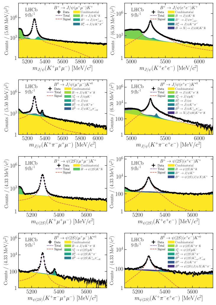
Figure 18: Invariant mass fit to the resonant control modes, from top to bottom: ${J\mskip-3.0mu/\mskip-2.0mu\psi}$ mode in ${{B}^{+}}\!\rightarrow{{K}^{+}}{\ell^{+}}{\ell^{-}}$, ${J\mskip-3.0mu/\mskip-2.0mu\psi}$ mode in ${{B}^{0}}\!\rightarrow{{K}^{*0}}{\ell^{+}}{\ell^{-}}$, $\psi{(2S)}$ mode in ${{B}^{+}}\!\rightarrow{{K}^{+}}{\ell^{+}}{\ell^{-}}$, $\psi{(2S)}$ in ${{B}^{0}}\!\rightarrow{{K}^{*0}}{\ell^{+}}{\ell^{-}}$. The muon (electron) modes are given on the left (right).

In common with previous LHCb analyses of LU, measurements of the relative decay rates of the resonant modes, $r_{{{J\mskip-3.0mu/\mskip-2.0mu\psi}}}^{K,{{K}^{*}}}$ and $R_{{\psi{(2S)}}}^{K,{{K}^{*}}}$, are used to validate the analysis procedure. The stability of $r_{{{J\mskip-3.0mu/\mskip-2.0mu\psi}}}^{K,{{K}^{*}}}$, measured as a function of different kinematic and geometric properties of the decays, both validates the analysis procedure and allows to quantify residual inaccuracies in the analysis chain and to assign systematic uncertainties. The compatibility of the ${{B}^{+}}$ and ${B}^{0}$ simulation calibrations is demonstrated by performing all cross-checks using both calibration chains. In addition, the cross-checks are repeated using the $\textrm{TOS}_{\textrm{inc}}$ trigger category, for which TOS is the primary trigger category and no requirements are imposed on the TIS classification of events.

The single ratios $r_{{{J\mskip-3.0mu/\mskip-2.0mu\psi}}}^{{K}}$ and $r_{{{J\mskip-3.0mu/\mskip-2.0mu\psi}}}^{{{K}^{*}}}$ are sensitive to residual imperfections in the simulation of electron and muon mode efficiencies, as well as those in the modeling of the resonant modes in the invariant mass fit. These ratios are expected to be equal to unity in the SM and have been determined precisely in previous measurements. Corrections can arise at the per mille level from the wider $q^{2}$ range in the electron mode, which could affect the decay rate due to subleading contributions from the FCNC process. Agreement of the $r_{{{J\mskip-3.0mu/\mskip-2.0mu\psi}}}^{{K}}$ and $r_{{{J\mskip-3.0mu/\mskip-2.0mu\psi}}}^{{{K}^{*}}}$ ratio with predictions of the SM, compatibility between data-taking periods, trigger categories, and when computed with the ${{B}^{+}}$ or the ${B}^{0}$ simulation correction was a prerequisite to evaluating the $R_{(K,{{K}^{*}})}$ observables. The ratios $R_{{\psi{(2S)}}}^{{K}}$ and $R_{{\psi{(2S)}}}^{{{K}^{*}}}$ are also used to validate that residual imperfections in the computation of efficiencies indeed cancel in the double muon-electron ratio.

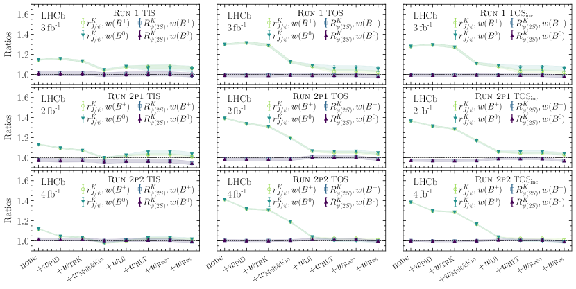
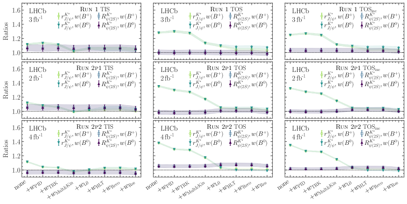
Figure 19: Evolution of the $r_{{{J\mskip-3.0mu/\mskip-2.0mu\psi}}}^{{K}}$ single and $R_{{\psi{(2S)}}}^{{K}}$ double ratios with each step of the simulation calibration procedure as labeled on the $x$-axis. The data-taking period and trigger category are indicated in the legend of each plot.

Figure 20: Evolution of the $r_{{{J\mskip-3.0mu/\mskip-2.0mu\psi}}}^{{{K}^{*}}}$ single and $R_{{\psi{(2S)}}}^{{{K}^{*}}}$ double ratio with each step of the simulation calibration procedure as labeled on the $x$-axis. The data-taking period and trigger category are indicated in the legend of each plot.

All invariant mass fits are performed constraining the invariant mass of the dilepton system to the ${J\mskip-3.0mu/\mskip-2.0mu\psi}$ or $\psi{(2S)}$ mass, as appropriate, where $m_{J/\psi}$ and $m_{\psi(2S)}$ labels denote the application of constraints on the dilepton system. The fits to data are illustrated in Fig. 18. The cross-check results are presented in Table 8 and shown in Fig. 20 and Fig. 20 for the ${{B}^{+}}$ and ${B}^{0}$, respectively, where only systematic uncertainties associated to the simulation sample and calibration sample statistics are included. Figures 20 and 20 also show the incremental effect of corrections to simulation in the determination of $r_{{{J\mskip-3.0mu/\mskip-2.0mu\psi}}}^{K,{{K}^{*}}}$. The uncertainties are dominated by the bootstrapping uncertainty on the simulation calibrations. As expected, both the single and double ratios are compatible with unity in all cases. The single ratio is incompatible with unity for the uncalibrated simulation, and its compatibility improves gradually as each calibration is applied. In contrast, the double ratio is compatible with unity from the outset and is practically unaffected by the calibrations applied to simulation.

Table 8: Values of the $r_{{{J\mskip-3.0mu/\mskip-2.0mu\psi}}}^{{K}}$ and $r_{{{J\mskip-3.0mu/\mskip-2.0mu\psi}}}^{{{K}^{*}}}$ single ratios, as well as $R_{{\psi{(2S)}}}^{{K}}$ and $R_{{\psi{(2S)}}}^{{{K}^{*}}}$ double ratios, calculated in different data-taking periods, trigger categories, and using the $w({{{B}^{+}}})$ or $w({{B}^{0}})$ calibration chains. The three uncertainties are, from left to right: statistical from the invariant mass fits, statistical from the finite simulated sample sizes, and the bootstrapping uncertainty on the simulation calibrations.

Sample	$r_{{{J\mskip-3.0mu/\mskip-2.0mu\psi}}}^{{K}}$	$r_{{{J\mskip-3.0mu/\mskip-2.0mu\psi}}}^{{{K}^{*}}}$
Run 1p1 $\textrm{TIS\phantom{O}}_{\textrm{\phantom{inc}}}$ $w({{{B}^{+}}})$	$1.063\pm 0.005\pm 0.003\pm 0.015$	$1.046\pm 0.010\pm 0.004\pm 0.016$
Run 1p1 $\textrm{TIS\phantom{O}}_{\textrm{\phantom{inc}}}$ $w({{B}^{0}})$	$1.054\pm 0.005\pm 0.003\pm 0.028$	$1.038\pm 0.010\pm 0.004\pm 0.027$
Run 1p1 $\textrm{TOS\phantom{I}}_{\textrm{\phantom{inc}}}$ $w({{{B}^{+}}})$	$1.020\pm 0.004\pm 0.003\pm 0.017$	$1.033\pm 0.008\pm 0.004\pm 0.018$
Run 1p1 $\textrm{TOS\phantom{I}}_{\textrm{\phantom{inc}}}$ $w({{B}^{0}})$	$1.053\pm 0.004\pm 0.003\pm 0.025$	$1.065\pm 0.008\pm 0.004\pm 0.025$
Run 1p1 $\textrm{TOS}_{\textrm{inc}}\textrm{\phantom{I}}$ $w({{{B}^{+}}})$	$1.021\pm 0.004\pm 0.002\pm 0.016$	$1.026\pm 0.007\pm 0.003\pm 0.017$
Run 1p1 $\textrm{TOS}_{\textrm{inc}}\textrm{\phantom{I}}$ $w({{B}^{0}})$	$1.056\pm 0.004\pm 0.002\pm 0.025$	$1.061\pm 0.007\pm 0.003\pm 0.024$
Run 2p1 $\textrm{TIS\phantom{O}}_{\textrm{\phantom{inc}}}$ $w({{{B}^{+}}})$	$1.010\pm 0.004\pm 0.003\pm 0.009$	$1.003\pm 0.008\pm 0.004\pm 0.010$
Run 2p1 $\textrm{TIS\phantom{O}}_{\textrm{\phantom{inc}}}$ $w({{B}^{0}})$	$1.033\pm 0.004\pm 0.003\pm 0.019$	$1.028\pm 0.008\pm 0.004\pm 0.018$
Run 2p1 $\textrm{TOS\phantom{I}}_{\textrm{\phantom{inc}}}$ $w({{{B}^{+}}})$	$1.035\pm 0.004\pm 0.003\pm 0.010$	$1.022\pm 0.007\pm 0.005\pm 0.010$
Run 2p1 $\textrm{TOS\phantom{I}}_{\textrm{\phantom{inc}}}$ $w({{B}^{0}})$	$1.046\pm 0.004\pm 0.003\pm 0.012$	$1.033\pm 0.007\pm 0.005\pm 0.012$
Run 2p1 $\textrm{TOS}_{\textrm{inc}}\textrm{\phantom{I}}$ $w({{{B}^{+}}})$	$1.030\pm 0.003\pm 0.002\pm 0.010$	$1.017\pm 0.006\pm 0.004\pm 0.010$
Run 2p1 $\textrm{TOS}_{\textrm{inc}}\textrm{\phantom{I}}$ $w({{B}^{0}})$	$1.039\pm 0.003\pm 0.002\pm 0.012$	$1.028\pm 0.006\pm 0.004\pm 0.012$
Run 2p2 $\textrm{TIS\phantom{O}}_{\textrm{\phantom{inc}}}$ $w({{{B}^{+}}})$	$1.012\pm 0.003\pm 0.003\pm 0.007$	$1.011\pm 0.006\pm 0.005\pm 0.007$
Run 2p2 $\textrm{TIS\phantom{O}}_{\textrm{\phantom{inc}}}$ $w({{B}^{0}})$	$1.016\pm 0.003\pm 0.003\pm 0.012$	$1.016\pm 0.006\pm 0.005\pm 0.011$
Run 2p2 $\textrm{TOS\phantom{I}}_{\textrm{\phantom{inc}}}$ $w({{{B}^{+}}})$	$1.014\pm 0.003\pm 0.003\pm 0.006$	$1.009\pm 0.005\pm 0.006\pm 0.004$
Run 2p2 $\textrm{TOS\phantom{I}}_{\textrm{\phantom{inc}}}$ $w({{B}^{0}})$	$0.993\pm 0.003\pm 0.003\pm 0.007$	$0.990\pm 0.005\pm 0.006\pm 0.006$
Run 2p2 $\textrm{TOS}_{\textrm{inc}}\textrm{\phantom{I}}$ $w({{{B}^{+}}})$	$1.014\pm 0.002\pm 0.003\pm 0.006$	$1.006\pm 0.004\pm 0.005\pm 0.005$
Run 2p2 $\textrm{TOS}_{\textrm{inc}}\textrm{\phantom{I}}$ $w({{B}^{0}})$	$0.991\pm 0.002\pm 0.003\pm 0.007$	$0.985\pm 0.004\pm 0.005\pm 0.007$
Sample	$R_{{\psi{(2S)}}}^{{K}}$	$R_{{\psi{(2S)}}}^{{{K}^{*}}}$
Run 1p1 $\textrm{TIS\phantom{O}}_{\textrm{\phantom{inc}}}$ $w({{{B}^{+}}})$	$0.993\pm 0.021\pm 0.005\pm 0.001$	$1.051\pm 0.044\pm 0.009\pm 0.002$
Run 1p1 $\textrm{TIS\phantom{O}}_{\textrm{\phantom{inc}}}$ $w({{B}^{0}})$	$0.996\pm 0.021\pm 0.005\pm 0.001$	$1.053\pm 0.044\pm 0.009\pm 0.002$
Run 1p1 $\textrm{TOS\phantom{I}}_{\textrm{\phantom{inc}}}$ $w({{{B}^{+}}})$	$0.979\pm 0.016\pm 0.004\pm 0.002$	$0.988\pm 0.033\pm 0.007\pm 0.002$
Run 1p1 $\textrm{TOS\phantom{I}}_{\textrm{\phantom{inc}}}$ $w({{B}^{0}})$	$0.982\pm 0.016\pm 0.004\pm 0.003$	$0.990\pm 0.033\pm 0.007\pm 0.004$
Run 1p1 $\textrm{TOS}_{\textrm{inc}}\textrm{\phantom{I}}$ $w({{{B}^{+}}})$	$0.980\pm 0.014\pm 0.003\pm 0.001$	$1.018\pm 0.029\pm 0.006\pm 0.003$
Run 1p1 $\textrm{TOS}_{\textrm{inc}}\textrm{\phantom{I}}$ $w({{B}^{0}})$	$0.983\pm 0.014\pm 0.003\pm 0.002$	$1.020\pm 0.029\pm 0.006\pm 0.003$
Run 2p1 $\textrm{TIS\phantom{O}}_{\textrm{\phantom{inc}}}$ $w({{{B}^{+}}})$	$0.945\pm 0.017\pm 0.004\pm 0.001$	$1.030\pm 0.039\pm 0.008\pm 0.002$
Run 2p1 $\textrm{TIS\phantom{O}}_{\textrm{\phantom{inc}}}$ $w({{B}^{0}})$	$0.947\pm 0.017\pm 0.004\pm 0.001$	$1.032\pm 0.039\pm 0.008\pm 0.002$
Run 2p1 $\textrm{TOS\phantom{I}}_{\textrm{\phantom{inc}}}$ $w({{{B}^{+}}})$	$0.986\pm 0.014\pm 0.003\pm 0.003$	$0.991\pm 0.029\pm 0.006\pm 0.004$
Run 2p1 $\textrm{TOS\phantom{I}}_{\textrm{\phantom{inc}}}$ $w({{B}^{0}})$	$0.987\pm 0.014\pm 0.003\pm 0.003$	$0.993\pm 0.029\pm 0.006\pm 0.005$
Run 2p1 $\textrm{TOS}_{\textrm{inc}}\textrm{\phantom{I}}$ $w({{{B}^{+}}})$	$0.969\pm 0.012\pm 0.003\pm 0.002$	$1.004\pm 0.025\pm 0.006\pm 0.003$
Run 2p1 $\textrm{TOS}_{\textrm{inc}}\textrm{\phantom{I}}$ $w({{B}^{0}})$	$0.970\pm 0.012\pm 0.003\pm 0.002$	$1.006\pm 0.025\pm 0.006\pm 0.004$
Run 2p2 $\textrm{TIS\phantom{O}}_{\textrm{\phantom{inc}}}$ $w({{{B}^{+}}})$	$0.992\pm 0.013\pm 0.004\pm 0.001$	$0.954\pm 0.025\pm 0.006\pm 0.001$
Run 2p2 $\textrm{TIS\phantom{O}}_{\textrm{\phantom{inc}}}$ $w({{B}^{0}})$	$0.994\pm 0.013\pm 0.004\pm 0.001$	$0.956\pm 0.025\pm 0.006\pm 0.001$
Run 2p2 $\textrm{TOS\phantom{I}}_{\textrm{\phantom{inc}}}$ $w({{{B}^{+}}})$	$0.999\pm 0.010\pm 0.003\pm 0.002$	$1.059\pm 0.023\pm 0.006\pm 0.002$
Run 2p2 $\textrm{TOS\phantom{I}}_{\textrm{\phantom{inc}}}$ $w({{B}^{0}})$	$1.000\pm 0.010\pm 0.003\pm 0.002$	$1.060\pm 0.023\pm 0.006\pm 0.002$
Run 2p2 $\textrm{TOS}_{\textrm{inc}}\textrm{\phantom{I}}$ $w({{{B}^{+}}})$	$0.993\pm 0.009\pm 0.003\pm 0.001$	$1.020\pm 0.018\pm 0.005\pm 0.002$
Run 2p2 $\textrm{TOS}_{\textrm{inc}}\textrm{\phantom{I}}$ $w({{B}^{0}})$	$0.994\pm 0.009\pm 0.003\pm 0.001$	$1.022\pm 0.018\pm 0.005\pm 0.002$

The stability of the single ratios $r_{{{J\mskip-3.0mu/\mskip-2.0mu\psi}}}^{{K}}$ and $r_{{{J\mskip-3.0mu/\mskip-2.0mu\psi}}}^{{{K}^{*}}}$ is tested by repeating the single-ratio cross-check as a function of 44 quantities related to the kinematics, geometry, or vertex quality of the decay, as well as to the event occupancy. For each quantity, the data are divided into eight intervals, each with comparable statistical precision on the single ratios. If the simulation is perfectly calibrated, the dependence on each quantity will be compatible with a straight line with slope zero and intercept one. Residual imperfections do not necessarily indicate a bias in the LU observables as long as the underlying distribution of the quantity in question is similar between the low-, central-, and ${{J\mskip-3.0mu/\mskip-2.0mu\psi}}$-${q^{2}}$ regions. Figure 21 shows the stability of $r_{{{J\mskip-3.0mu/\mskip-2.0mu\psi}}}^{{K}}$ and $r_{{{J\mskip-3.0mu/\mskip-2.0mu\psi}}}^{{{K}^{*}}}$ as a function of the dilepton opening angle $\theta(\ell^{+}\ell^{-})$, one of the quantities whose distribution is most different between the low-, central-, and ${J\mskip-3.0mu/\mskip-2.0mu\psi}$-$q^{2}$ regions. The potential for small residual bias to be reflected on the LU observables is evaluated and discussed in Section 9.

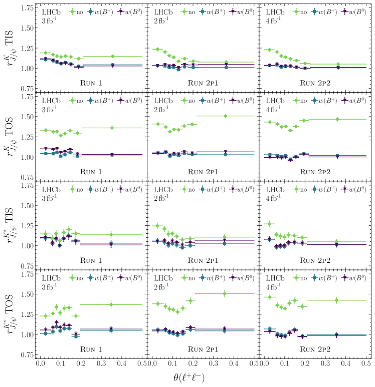
Figure 21: Values of the $r_{{{J\mskip-3.0mu/\mskip-2.0mu\psi}}}^{{K}}$ and $r_{{{J\mskip-3.0mu/\mskip-2.0mu\psi}}}^{{{K}^{*}}}$ single ratios as a function of the dilepton opening angle $\theta(\ell^{+}\ell^{-})$. From top to bottom: $r_{{{J\mskip-3.0mu/\mskip-2.0mu\psi}}}^{{K}}$ TIS, $r_{{{J\mskip-3.0mu/\mskip-2.0mu\psi}}}^{{K}}$ TOS, $r_{{{J\mskip-3.0mu/\mskip-2.0mu\psi}}}^{{{K}^{*}}}$ TIS, and $r_{{{J\mskip-3.0mu/\mskip-2.0mu\psi}}}^{{{K}^{*}}}$ TOS. From left to right: the Run 1, Run 2p1 and Run 2p2 data-taking periods. The ratios are shown without simulation calibrations, with ${{B}^{+}}$ calibrations, and with ${B}^{0}$ calibrations.

Finally the $r_{{{J\mskip-3.0mu/\mskip-2.0mu\psi}}}^{{K}}$ and $r_{{{J\mskip-3.0mu/\mskip-2.0mu\psi}}}^{{{K}^{*}}}$ single ratios, as well as $R_{{\psi{(2S)}}}^{{K}}$ and $R_{{\psi{(2S)}}}^{{{K}^{*}}}$ double ratios, are computed including all relevant systematic uncertainties described in Sec. 9. The two-dimensional likelihood scans are shown in Fig. 22. For likelihood scans of $R_{{\psi{(2S)}}}^{{K}}$, $R_{{\psi{(2S)}}}^{{{K}^{*}}}$, no systematic uncertainties on the fit model are included. Both the single and double ratios agree with the Standard Model predictions at better than two standard deviations.

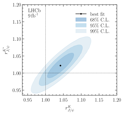
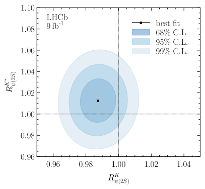
Figure 22: Two dimensional likelihood scans of (left) $r_{{{J\mskip-3.0mu/\mskip-2.0mu\psi}}}^{{K}}$ vs. $r_{{{J\mskip-3.0mu/\mskip-2.0mu\psi}}}^{{{K}^{*}}}$ and (right) $R_{{\psi{(2S)}}}^{{K}}$ vs. $R_{{\psi{(2S)}}}^{{{K}^{*}}}$. The contours show the 68%, 95% and 99% C.L. regions and the solid markers show the best fit values.

8.2 Stability of results with respect to PID criteria

To check the modeling of misidentified backgrounds, the nominal fit is performed without including these backgrounds. The fit is then repeated, progressively tightening the PID criteria. The results are shown in Fig. 23. The clear trends observed when loosening PID criteria demonstrate the importance of including these backgrounds in the nominal fit. Past a certain point, however, the fit results plateau in all four LU observables. When all uncertainties are taken into account, the fit values in this plateau region are fully compatible with the nominal fit result discussed in Sec. 10, where the misidentified backgrounds are explicitly modeled.

The same procedure is repeated at two working points while including the modeling of the backgrounds in the fit model. The results are shown in Fig. 24. Here the “intermediate” working point is $\textrm{DLL(e)}>3$ and $\textrm{ProbNN(e)}>0.4$, while the “tight” working point is $\textrm{DLL(e)}>5$ and $\textrm{ProbNN(e)}>0.5$, for comparison to Fig. 23. The overall expected contamination from misidentified backgrounds at the intermediate working point is half of the contamination at the nominal working point, while the contamination at the tight working point is expected to be nearly negligible. No trends are observed, giving confidence in the extrapolation and modeling of misidentified backgrounds in the fit.

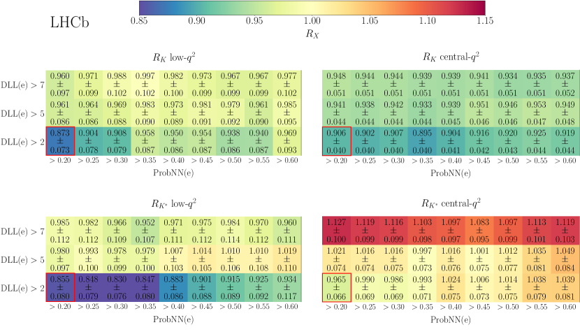
Figure 23: Results of the nominal fit without modeling of misidentified backgrounds as a function of the PID criteria used. The bins are, from top left to bottom right: $R_{K}$ low-$q^{2}$, $R_{K}$ $\text{central-}{q^{2}}$, $R_{{{K}^{*}}}$ $\text{low-}{q^{2}}$ and $R_{{{K}^{*}}}$ $\text{central-}{q^{2}}$. The nominal set of criteria is highlighted in red. The quoted uncertainties are statistical only.

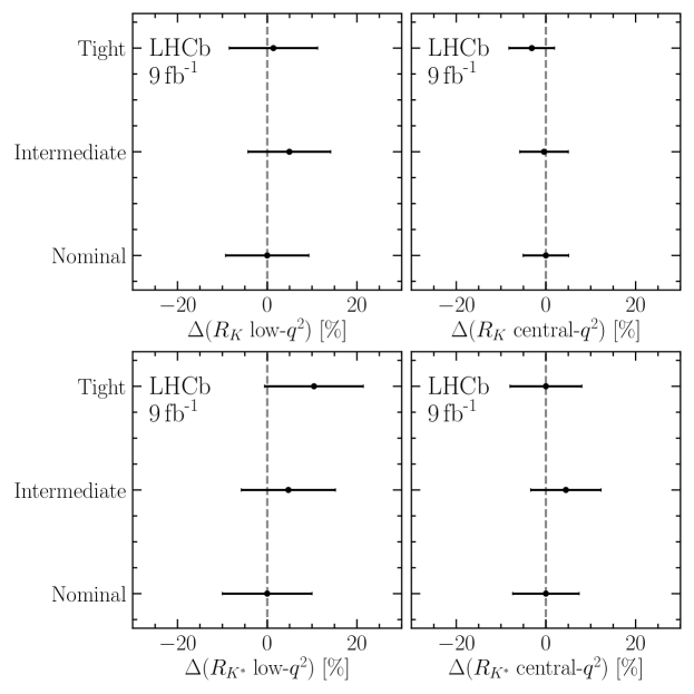
Figure 24: Shifts of the central value results from varying the PID criteria on electrons while modeling misidentified backgrounds in the fit. Particle selection criteria are varied to an intermediate working point reducing the expected contamination by a factor two, and to a tighter working point reducing the contamination by more than 75%. The bins are, from top left to right: $R_{K}$ low-$q^{2}$, $R_{K}$ $\text{central-}{q^{2}}$, $R_{{{K}^{*}}}$ $\text{low-}{q^{2}}$ and $R_{{{K}^{*}}}$ $\text{central-}{q^{2}}$. The quoted relative uncertainties are statistical only.

8.3 Study of ${{B}^{0}}\!\rightarrow{{K}^{*0}}{e^{+}e^{-}}$ at very low-$q^{2}$

As an additional test of the portability of efficiencies from the ${J\mskip-3.0mu/\mskip-2.0mu\psi}$ region to other $q^{2}$ regions, the branching fraction of the ${{B}^{0}}\!\rightarrow{{K}^{*0}}{e^{+}e^{-}}$ mode normalized to the ${B}^{0}$ resonant mode is measured [95] in the very $\text{low-}{q^{2}}$ region of $[0.0001,0.1]\text{\,Ge\kern-1.00006ptV}^{2}\!/c^{4}$. Since there are practically no relevant hadronic backgrounds in this $q^{2}$ region, this cross-check also further tests our understanding of misidentified backgrounds in the nominal analysis. The selection criteria and efficiency determination are the same as for the rest of the analysis. The measured branching fraction is determined to be equal to $(1.57\pm 0.12)\cdot 10^{-7}$, where the uncertainty includes only the statistical component. The result agrees perfectly with the SM prediction which has been evaluated multiplying the known world best average branching ratio of ${{B}^{0}}\!\rightarrow{{K}^{*0}}\gamma$ [51] to the ratio of decay rates of ${{B}^{0}}\!\rightarrow{{K}^{*0}}{e^{+}e^{-}}$ in the very $\text{low-}{q^{2}}$ and ${{B}^{0}}\!\rightarrow{{K}^{*0}}\gamma$. The latter has been evaluated using the flavio package [71]. Moreover no significant trends in the efficiency corrected yields are observed when varying the PID requirements.

9 Systematic uncertainties

Systematic uncertainties can be divided into two broad categories: those associated with the determination of the signal and control mode efficiencies that directly enter Eq. 2 and those associated with the simultaneous invariant mass fit. Bootstrapping uncertainties associated with the nominal calibration procedure are described in Sec. 6 and are considered separately from effects discussed further in this section.

Systematic uncertainties associated with efficiencies are generally determined by varying assumptions made in the calibration of simulated samples and measuring the corresponding shifts in $R_{K}$ and $R_{{{K}^{*}}}$. Systematic uncertainties associated with the fit model are generally determined by generating large ensembles of pseudoexperiments, varying assumptions made in the fit procedure, and measuring the corresponding shifts in $R_{K}$ and $R_{{{K}^{*}}}$ between the nominal and varied fit configuration. In both cases correlations are inferred from observing the coherence of the measured shifts. All systematic uncertainties are assumed to follow Gaussian distributions and are evaluated separately for each LU observable, data-taking period and trigger category. The correlations between observables, data-taking periods, and trigger categories are also evaluated for each source of systematic uncertainty. The final outcome is a $24\times 24$ covariance matrix that can be used as an additional constraint in the simultaneous fit to calculate the likelihood for each observable including both statistical and systematic uncertainties.

9.1 Systematic uncertainties on efficiencies

Truth-level information

The nominal analysis procedure associates reconstructed candidates in simulated events to the underlying “truth-level” information which describes which generated particles left hits in the LHCb detector. This association is used to filter out misreconstructed candidates and ensures that each PDF constructed from simulated events represents only the decay mode of interest for that PDF. The association criteria are varied and the efficiencies recomputed.

Multiple candidates

The results for $r_{{{J\mskip-3.0mu/\mskip-2.0mu\psi}}}^{{K}}$ and $r_{{{J\mskip-3.0mu/\mskip-2.0mu\psi}}}^{{{K}^{*}}}$ are recomputed keeping all candidates for each event, rather than selecting a single candidate at random. All deviations are found to be compatible with zero and no systematic uncertainty is therefore assigned.

Form factors used in simulation

The simulated samples used in this analysis are generated for ${{B}^{+}}$ and ${B}^{0}$ decays according to the form factor model given in Ref. [96]. These form factors affect both the signal efficiencies and the migration of events between $q^{2}$ regions. The associated systematic uncertainty is evaluated by deriving differential decay rates across $q^{2}$ and the decay angles defined as in Ref. [97], where only the efficiency dependence on the decay angle describing the lepton system is considered. The nominal form factors of Ref. [96] are then compared with those of Refs. [98] and [99], for the ${B}^{0}$ and ${{B}^{+}}$ decays respectively, by multiplying the resulting differential decay rate with the relevant efficiency distribution. The theory uncertainty on the differential decay rate for the form factors taken from Refs. [98, 99], is also propagated to the efficiency ratios, but the resulting deviation is found to be generally smaller than that due to the difference in central values between the two models.

Particle identification efficiencies

Systematic uncertainties associated with PID efficiencies arise from two sources: residual non-factorization of the electron efficiencies, and the binning scheme used to compute the PID efficiencies on data and simulation. The first effect is quantified by comparing efficiencies obtained from truth-level information with efficiencies obtained using the nominal calibration procedure on simulated signal samples. The binning scheme systematic is evaluated separately for muons, hadrons, and electrons. In the case of muons and hadrons a kernel density estimator is used to provide an unbinned efficiency parametrization in momentum and pseudorapidity, while the number of track multiplicity bins is varied. This is possible because the muon and hadron calibrations are derived from high-purity background-subtracted samples of charm hadron and charmonia decays, and the weights used to subtract background also allow a per-event efficiency to be determined.

Dielectron calibration samples have a lower purity because of bremsstrahlung, which also introduces correlations between the reconstructed dielectron mass and the properties of its constituent electrons, including their probability to pass a given PID criterion. Their efficiencies therefore have to be calculated using a fit-and-count approach in the defined binning scheme. For this reason no per-event background-subtracted efficiency can be determined and consequently no unbinned parametrization is possible. The systematic uncertainty is therefore derived by interpolating the binned efficiency maps and measuring the difference in efficiencies between this interpolated parametrization and the binned maps. The $p_{\mathrm{T}}$, pseudorapidity, and track multiplicity binning schemes are also varied. The factorization- and the binning scheme-effects are assumed to be uncorrelated when determining the overall systematic uncertainty.

Kinematic and multiplicity calibration

The $w_{\textrm{Mult\&Kin}}$ weights are re-evaluated in two ways: first using events in the TIS trigger category rather than the nominal approach of using events in the L0 muon TOS category, and second using as multiplicity proxy the number of tracks reconstructed in the vertex detector, rather than in the whole tracking system.

Trigger efficiencies

Systematic uncertainties on the L0 efficiencies are associated with the binning scheme, the use of muon mode TIS efficiencies as a proxy for the electron mode, and the factorization of electron TOS efficiencies. The binning systematic uncertainty is evaluated by measuring the difference in efficiencies between an interpolated parametrization and the binned maps. The TIS efficiencies are computed for the electron mode, and compared to the proxy efficiencies obtained from the muon mode. The factorization systematic uncertainty is evaluated by directly measuring the L0 dielectron TOS efficiencies instead of multiplying the nominal per-electron efficiencies.

Systematic uncertainties on the HLT efficiencies are associated with the binning scheme and the decision to parametrize the efficiency as a function of track multiplicity. The potential systematic uncertainty on the HLT efficiencies are estimated by parametrizing in terms of the $B$ hadron transverse momentum instead of track multiplicity and varying the binning scheme.

Stability of $r_{{{J\mskip-3.0mu/\mskip-2.0mu\psi}}}^{{K}}$ and $r_{{{J\mskip-3.0mu/\mskip-2.0mu\psi}}}^{{{K}^{*}}}$

The fact that the single ratios $r_{{{J\mskip-3.0mu/\mskip-2.0mu\psi}}}^{{K}}$ and $r_{{{J\mskip-3.0mu/\mskip-2.0mu\psi}}}^{{{K}^{*}}}$ are not perfectly flat when evaluated as a function of the properties of the corresponding ${J\mskip-3.0mu/\mskip-2.0mu\psi}$ control mode decay implies the presence of residual imperfections in the calibration of simulated samples. The corresponding systematic uncertainties on $R_{K}$ and $R_{{{K}^{*}}}$ are quantified with a flatness parameter, $d_{f}$, defined as

$$d_{f}=\left(\frac{\sum^{8}_{i}\varepsilon_{\text{Rare},\mu}^{i}\cdot\mathcal{Y}^{i}_{\mu}}{\sum^{8}_{i}\varepsilon_{\text{Rare},\mu}^{i}}\cdot\frac{\sum^{8}_{i}\varepsilon_{{{J\mskip-3.0mu/\mskip-2.0mu\psi}},\mu}^{i}}{\sum^{8}_{i}N^{i}_{\mu}}~{}\bigg{/}~{}\frac{\sum^{8}_{i}\varepsilon_{\text{Rare},e}^{i}\cdot\mathcal{Y}^{i}_{e}}{\sum^{8}_{i}\varepsilon_{\text{Rare},e}^{i}}\cdot\frac{\sum^{8}_{i}\varepsilon_{{{J\mskip-3.0mu/\mskip-2.0mu\psi}},e}^{i}}{\sum^{8}_{i}N^{i}_{e}}\right)-1,$$ (7)

where $\varepsilon^{i}_{\text{Rare},\ell}$ and $\epsilon^{i}_{{{J\mskip-3.0mu/\mskip-2.0mu\psi}},\ell}$ refer to the signal and control mode efficiencies in bin $i$ respectively; $N^{i}_{\ell}$ denotes the control mode yield measured in bin $i$; and $\mathcal{Y}^{i}_{\ell}$ is the efficiency corrected control mode yield in bin $i$,

$$\mathcal{Y}^{i}_{\ell}=\frac{N^{i}_{\ell}}{\varepsilon_{{{J\mskip-3.0mu/\mskip-2.0mu\psi}},\ell}^{i}}.$$ (8)

The $d_{f}$ parameter can be considered a proxy for the double ratios $R_{K}$ and $R_{{{K}^{*}}}$ in which the signal mode yields are replaced by the ${J\mskip-3.0mu/\mskip-2.0mu\psi}$ mode yields. The $d_{f}$ parameter is evaluated for each of the 44 quantities used to describe the ${J\mskip-3.0mu/\mskip-2.0mu\psi}$ control mode decay. The vast majority of the quantities considered result in $d_{f}$ values of a few per mille that are compatible with zero. The two quantities that show the greatest deviations from zero are the dilepton opening angle and the impact parameter $\chi^{2}$ of the dilepton system. The dilepton opening angle $d_{f}$ values are larger than those computed from the impact parameter $\chi^{2}$ of the dilepton system in all cases, and are consequently used to define the resulting systematic uncertainty.

9.2 Systematic uncertainties on the invariant mass fit

${J\mskip-3.0mu/\mskip-2.0mu\psi}$ mode fit model

The fidelity of the ${J\mskip-3.0mu/\mskip-2.0mu\psi}$ mode fit model is limited by the knowledge of the numerous partially reconstructed backgrounds that contribute to the region below the nominal $B$ mass. This is a particular problem for the ${J\mskip-3.0mu/\mskip-2.0mu\psi}$ mode because of partially reconstructed backgrounds, such as those with a ${\psi{(2S)}}\rightarrow{{J\mskip-3.0mu/\mskip-2.0mu\psi}}\pi\pi$ decay chain, which have no analogue in the signal mode. Although partially reconstructed backgrounds have missing energy and should therefore be located only below the nominal $B$ mass, poorly reconstructed candidates or candidates with wrongly associated bremsstrahlung photons cause a long tail towards higher $B$ masses. Since the statistical sensitivity of the fit, as seen from Table 8, is at the few per mille level, even contributions with mismodeling below the percent level can lead to a significant systematic uncertainty. It is particularly important to evaluate this systematic uncertainty with care because the fit is fully correlated between the low- and central-$q^{2}$ measurements of $R_{K}$ and $R_{{{K}^{*}}}$. The results of four fits to the invariant mass of the ${J\mskip-3.0mu/\mskip-2.0mu\psi}$ mode are compared:

1. The nominal fits used for the measurement of the $R_{K}$ and $R_{{{K}^{*}}}$ double ratios, without any constraint on the dilepton invariant mass;

2. Fits without a constraint on the dilepton invariant mass in which the partially reconstructed backgrounds in the electron mode are minimized by requiring that the $B$ candidate invariant mass is greater than 5200$\text{\,Me\kern-1.00006ptV\!/}c^{2}$ when the dilepton invariant mass is constrained to the ${J\mskip-3.0mu/\mskip-2.0mu\psi}$ mass;

3. The fits with a constraint on the dilepton invariant mass used for all the results given in Sec. 8;

4. The same as 3. but extending the lower fit range of the electron mode to 4650$\text{\,Me\kern-1.00006ptV\!/}c^{2}$, in order to test the sculpting of the partially reconstructed background PDFs induced by the 6$\text{\,Ge\kern-1.00006ptV}^{2}\!/c^{4}$ lower limit on the dielectron $q^{2}$;

These fits are grouped into two categories in order to assign a systematic uncertainty. Differences between 1. and 3. probe uncertainties related to imperfect signal modeling, to the choice of fit range, and to residual partially reconstructed backgrounds which peak under the signal when the dilepton mass is constrained but not otherwise. Differences between 2. and 4. probe uncertainties due to the imperfect composition of the partially reconstructed background cocktails. These two differences are added together in quadrature to obtain a total systematic uncertainty for the modeling and fitting of the ${J\mskip-3.0mu/\mskip-2.0mu\psi}$ mode. These differences are also taken to accommodate uncertainties associated with the finite simulated samples used to derive background PDFs, since changes in the background templates between constrained and unconstrained fits are far bigger than any statistical variation.

Fixed fit parameters

In the fit, parameters that are fixed, rather than constrained, are varied within their uncertainty in pseudoexperiments, and a corresponding systematic uncertainty calculated. The fraction of electron signals in each bremsstrahlung category is studied as a function of data-taking periods, trigger categories, and the transverse momentum and pseudorapidity of the $B$ meson. The fraction of events with a single bremsstrahlung photon is found to be $(50\pm 1)\%$ in all cases, with differences in the rate of bremsstrahlung photon emission or in their detection efficiency causing a migration of events from the zero photon category to the two-or-more photon category and vice versa. A systematic uncertainty is assigned by varying the fraction of events in the zero and two-or-more bremsstrahlung categories by $\pm 1\%$ in pseudoexperiments and observing the resulting change on the $R_{K}$ and $R_{{{K}^{*}}}$ double ratios.

Specific backgrounds

The shape of the ${{B}^{+}}\!\rightarrow{{K}^{+}}{{\pi}^{+}}{{\pi}^{-}}{e^{+}e^{-}}$ decay modeled in the ${{B}^{0}}\!\rightarrow{{K}^{*0}}{e^{+}e^{-}}$ mass fits depends on the amplitude model assumed for the ${{K}^{+}}{{\pi}^{+}}{{\pi}^{-}}$ system. The simulated events used in this analysis are generated with a phase-space distribution of ${{K}^{+}}{{\pi}^{+}}{{\pi}^{-}}$ masses. It has been checked that weighting the $m({{K}^{+}}{{\pi}^{+}}{{\pi}^{-}})$, $m({{K}^{+}}{{\pi}^{-}})$ and $m({{\pi}^{+}}{{\pi}^{-}})$ distributions to match those obtained from efficiency corrected and background-subtracted ${{B}^{+}}\!\rightarrow{{K}^{+}}{{\pi}^{+}}{{\pi}^{-}}{{J\mskip-3.0mu/\mskip-2.0mu\psi}}(\!\rightarrow{\mu^{+}\mu^{-}})$ data does not impact the modeling of the background after all selections are applied.

A second study, to evaluate the effect on angular structures, is performed generating dedicated samples of ${{B}^{+}}\!\rightarrow{{K}^{+}}{{\pi}^{+}}{{\pi}^{-}}{e^{+}e^{-}}$ including the $K^{+}_{1}$ and $K^{*+}_{2}$ resonances, and once again the ${{K}^{+}}{{\pi}^{-}}{e^{+}}{e^{-}}$ mass distribution is found to be compatible. Pseudoexperiments are used to confirm that the systematic uncertainty associated with residual differences in the mass distribution are negligibly small. Further residual differences in mass shapes between the ${{B}^{+}}\!\rightarrow{{K}^{+}}{{\pi}^{+}}{{\pi}^{-}}{e^{+}e^{-}}$ and ${{B}^{0}}\rightarrow{{K}^{+}}{{\pi}^{-}}{{\pi}^{0}}{e^{+}e^{-}}$ backgrounds, which could be caused by isospin-breaking effects, are also negligible due to the detector resolution.

The relative normalizations of the different physics processes which contribute to the $B^{+,0}\rightarrow(K\pi)^{+,0}{e^{+}}{e^{-}}$ background in the ${{B}^{+}}\!\rightarrow{{K}^{+}}{e^{+}e^{-}}$ invariant mass are varied within the uncertainties given in Sec. 7.1. Pseudoexperiment studies are used to determine the systematic uncertainties on $R_{K}$ and $R_{{{K}^{*}}}$ associated with these variations.

Systematic uncertainties are calculated for the invariant mass shapes and expected yields of misidentified backgrounds. One group of systematic uncertainties concerns the PID weights used to extrapolate from the control region to the nominal fit region. The binning of the calibration histograms used to compute these weights is varied, the weights are parameterised in particle momentum instead of transverse momentum, and an additional correction for the detector occupancy is applied. A second type of systematic uncertainties concerns the definition of inverted PID criteria which define the control region. Four different variations are evaluated and the biggest observed difference taken as a systematic uncertainty. In addition, the threshold used to define a control region event as pion- or kaon-like is varied from the nominal approach of a very pure sample of pion-like events to an alternative choice of a very pure sample of kaon-like events. Finally, the invariant mass shape of the misidentified backgrounds is evaluated using an alternative model based on unbinned templates.

9.3 Overall systematic uncertainties

The individual sources of systematic uncertainty on $R_{K}$ and $R_{{{K}^{*}}}$ are reported in Table 9. The dominant source of systematic uncertainty comes from the treatment of misidentified backgrounds in the fit model. Nevertheless the systematic uncertainties remain significantly smaller than the statistical uncertainties. Moreover, the dominant sources of systematic uncertainty arise from the finite size of control samples and are therefore themselves statistical in nature. They will consequently decrease in future analyses based on larger data samples.

Table 9: Sources of systematic uncertainties on the $R_{K}$ and $R_{{{K}^{*}}}$ measurements in the low- and $\text{central-}{q^{2}}$ regions. All values are given in percent and relative to the measured central value. These values are indicative and are computed as weighted averages of systematic variations determined in each data-taking period and trigger category. The different sources of uncertainties are determined using a best linear unbiased estimator accounting for correlations between different data taking periods and trigger categories. The bottom row with the total systematic is estimated by combining the error matrices for each source in quadrature and performing a best linear unbiased estimation.

Source	$\text{low-}{q^{2}}$ $R_{K}$	$\text{central-}{q^{2}}$ $R_{K}$	$\text{low-}{q^{2}}$ $R_{{{K}^{*}}}$	$\text{central-}{q^{2}}$ $R_{{{K}^{*}}}$
Form factors	0.09	0.08	0.83	0.76
$q^{2}$ smearing	0.30	0.19	0.28	0.31
Particle identification	0.17	0.22	0.10	0.12
Kinematics and multiplicity	0.35	0.26	0.57	0.52
Trigger	0.27	0.16	0.26	0.13
Stability of $r_{{{J\mskip-3.0mu/\mskip-2.0mu\psi}}}^{{K}}$ and $r_{{{J\mskip-3.0mu/\mskip-2.0mu\psi}}}^{{{K}^{*}}}$	0.78	0.38	1.79	0.47
${J\mskip-3.0mu/\mskip-2.0mu\psi}$ fit model	0.35	0.35	0.40	0.40
Fixed fit parameters	0.14	0.07	0.25	0.16
Combinatorial shape	0.99	0.16	1.39	0.38
Specific backgrounds	0.24	0.20	1.24	0.51
Misidentified backgrounds	2.50	2.22	1.87	2.29
Modeling of $m_{\mathrm{corr}}$	0.25	0.24	0.33	0.33
Total	2.86	2.33	3.73	2.52

10 Results

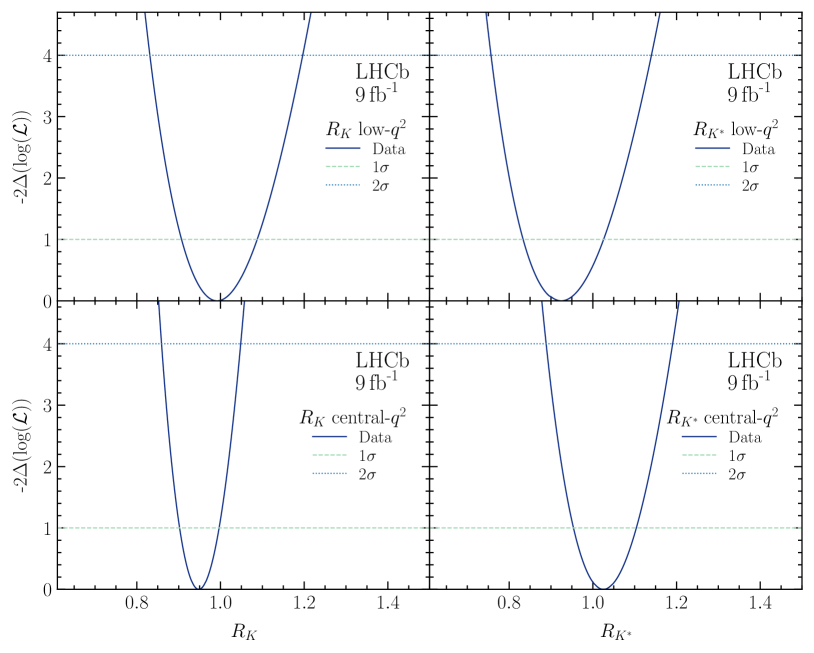
Figure 25: Likelihood scans for the LU observables (left) $R_{K}$ and (right) $R_{{{K}^{*}}}$, in the (top) $\text{low-}{q^{2}}$ and (bottom) $\text{central-}{q^{2}}$ regions.

The best fit point together with the statistical and systematic uncertainties for the four LU observables are reported in Table 10. The results for each running period, given in App. A, are consistent with each other and with the overall result. Each of the four relative branching fraction measurements is the most precise to date. The uncertainties on the lepton universality observables are not Gaussian due to the finite sample sizes used in this analysis. Likelihood scans for each of the double-ratio LU observables are presented in Fig. 25. The likelihood scans are used to derive the asymmetric uncertainties reported in Table 10. The correlation matrix reported by the fit to data including all uncertainties is shown in Fig. 26. In order to separate statistical and systematic uncertainties the likelihood scans are performed twice, once with and once without the systematic uncertainties included in the fit covariance matrix. The uncertainties of these are then subtracted in quadrature to obtain the contribution of systematic uncertainties to the overall uncertainty.

Table 10: Measured values of the $R_{K}$ and $R_{{{K}^{*}}}$ observables in the low- and $\text{central-}{q^{2}}$ regions, with the associated statistical and systematic uncertainties presented separately.

low-$q^{2}$ $R_{K}$	central-$q^{2}$ $R_{K}$	low-$q^{2}$ $R_{{{K}^{*}}}$	central-$q^{2}$ $R_{{{K}^{*}}}$
$0.994\,^{+0.090}_{-0.082}\,{}^{+0.029}_{-0.027}$	$0.949\,^{+0.042}_{-0.041}\,{}^{+0.022}_{-0.022}$	$0.927\,^{+0.093}_{-0.087}\,{}^{+0.036}_{-0.035}$	$1.027\,^{+0.072}_{-0.068}\,{}^{+0.027}_{-0.026}$

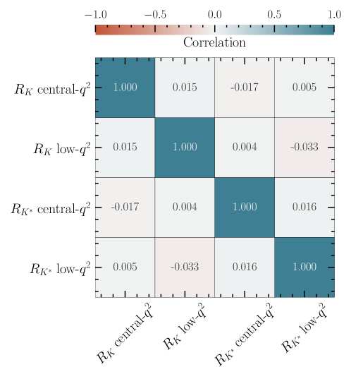
Figure 26: Correlation factors between the $R_{K}$ and $R_{{{K}^{*}}}$ results in the low- and $\text{central-}{q^{2}}$ regions.

The sPlot [100] technique is used to obtain background-subtracted distributions of quantities describing the ${B}^{0}$ and ${B}^{+}$ decays in the four $q^{2}$ regions considered. The simulation is used to verify that this technique allows the quantities in question to be determined accurately, despite the fact that bremsstrahlung causes significant correlations between $q^{2}$ and the mass of the $B$ meson candidate for both the electron signal and for the backgrounds. Figure 27 shows the resulting distributions.

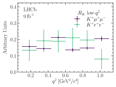
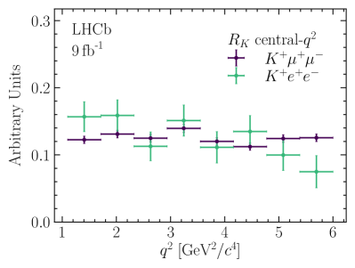
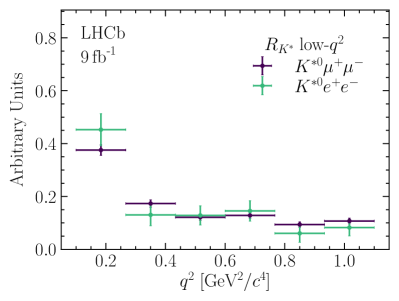
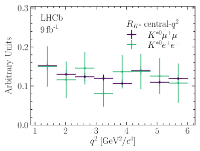
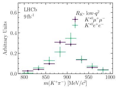
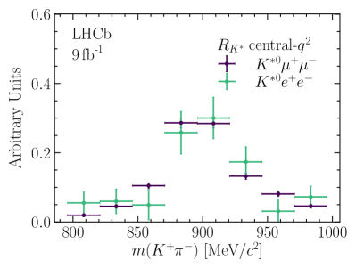
Figure 27: Background-subtracted distributions of quantities describing the ${{B}^{+}}\rightarrow{{K}^{+}}\ell^{+}\ell^{-}$ and ${{B}^{0}}\rightarrow{{K}^{*0}}\ell^{+}\ell^{-}$ decays. The $\text{low-}{q^{2}}$ region is plotted on the left, the $\text{central-}{q^{2}}$ region on the right. The top and middle rows show the distributions of $q^{2}$ for the ${{B}^{+}}$ and ${B}^{0}$ signals, respectively. The bottom row shows the distribution of the ${K}^{*0}$ mass for the ${B}^{0}$ signals.

The LU results are used to calculate the differential branching fractions of ${{B}^{+}}\!\rightarrow{{K}^{+}}{e^{+}e^{-}}$ and ${{B}^{0}}\!\rightarrow{{K}^{*0}}{e^{+}e^{-}}$ decays, averaged over the central $q^{2}$ region. This is done by combining the $R_{K}$ and $R_{{{K}^{*}}}$ measurements at central $q^{2}$ with the known ${{B}^{+}}\!\rightarrow{{K}^{+}}{\mu^{+}\mu^{-}}$ [49] and ${{B}^{0}}\!\rightarrow{{K}^{*0}}{\mu^{+}\mu^{-}}$ [54] branching fractions; in the latter case, only the ${{K}^{*}}(892)^{0}$ P-wave state is considered. Similar results are not obtained in the $\text{low-}{q^{2}}$ region since the muonic branching fractions are not available in the same $q^{2}$ range as used in this analysis. All systematic uncertainties on the LU ratios are assumed to be correlated with the systematic uncertainties on the branching fractions, with the exception of the effect induced by the normalization channel; this is taken to be uncorrelated. The correlations between the statistical uncertainties of the LU observables and the branching fractions are evaluated based on the overlap between ${{B}^{+}}\!\rightarrow{{K}^{+}}{\mu^{+}\mu^{-}}$ and ${{B}^{0}}\!\rightarrow{{K}^{*0}}{\mu^{+}\mu^{-}}$ data sets used in either measurements. It is found that 61% of the ${{B}^{+}}\!\rightarrow{{K}^{+}}{\mu^{+}\mu^{-}}$ Run 1 sample was used in the corresponding branching-fraction measurement, whereas for ${{B}^{0}}\!\rightarrow{{K}^{*0}}{\mu^{+}\mu^{-}}$ this overlap is 69%. Combined with the Run 2 yields, this leads to a correlation of 0.13 between the statistical uncertainties of the ${{B}^{+}}\!\rightarrow{{K}^{+}}{\mu^{+}\mu^{-}}$ branching fraction measurement and this LU measurement. We similarly find a correlation of 0.14 between the ${{B}^{0}}\!\rightarrow{{K}^{*0}}{\mu^{+}\mu^{-}}$ statistical uncertainties. The electron mode branching fractions, averaged over the $\text{central-}{q^{2}}$ region, are found to be

$$\frac{\mathrm{d}\mathcal{B}({{B}^{+}}\!\rightarrow{{K}^{+}}{e^{+}e^{-}})}{\mathrm{d}{q^{2}}} =(25.5^{+1.3}_{-1.2}\pm 1.1)\times 10^{-9}\,\text{\,Ge\kern-1.00006ptV}^{-2}$$

$$\frac{\mathrm{d}\mathcal{B}({{B}^{0}}\!\rightarrow{{K}^{*0}}{e^{+}e^{-}})}{\mathrm{d}{q^{2}}} =(33.3^{+2.7}_{-2.6}\pm 2.2)\times 10^{-9}\,\text{\,Ge\kern-1.00006ptV}^{-2}.$$

11 Conclusion

We present the first simultaneous test of LU in ${{B}^{+}}\!\rightarrow{{K}^{+}}{\ell^{+}}{\ell^{-}}$ and ${{B}^{0}}\!\rightarrow{{K}^{*0}}{\ell^{+}}{\ell^{-}}$ decays using all $pp$ collision data collected with the LHCb detector between 2011 and 2018, corresponding to an integrated luminosity of 9$\text{\,fb}^{-1}$. The ratios of the branching fractions of muon and electron modes are measured in both channels and in two ranges of the square of the dilepton invariant mass. Each of these four measurements is either the first ($R_{K}$ low-$q^{2}$) or the most precise ($R_{{{K}^{*}}}$ low-$q^{2}$, $R_{K}$ central-$q^{2}$ and $R_{{{K}^{*}}}$ central-$q^{2}$) such measurement to date. The measured values are

$$\text{low-}{q^{2}}\begin{cases}R_{K}&=0.994~{}^{+0.090}_{-0.082}\text{\,(stat)}\;^{+0.029}_{-0.027}\text{\,(syst)},\\ R_{{{K}^{*}}}&=0.927~{}^{+0.093}_{-0.087}\text{\,(stat)}\;^{+0.036}_{-0.035}\text{\,(syst)},\\ \end{cases}$$

$$\text{central-}{q^{2}}\begin{cases}R_{K}&=0.949~{}^{+0.042}_{-0.041}\text{\,(stat)}\;^{+0.022}_{-0.022}\text{\,(syst)},\\ R_{{{K}^{*}}}&=1.027~{}^{+0.072}_{-0.068}\text{\,(stat)}\;^{+0.027}_{-0.026}\text{\,(syst)},\end{cases}$$

where the first uncertainty in each row is statistical and the second systematic.

The central values of the SM prediction, as calculated by the flavio software package [71], are given in Table 11. An additional uncertainty of 1% is assigned to take into account uncertainties in the modeling of QED effects in ${{B}^{+}}\!\rightarrow{{K}^{+}}{\ell^{+}}{\ell^{-}}$ and ${{B}^{0}}\!\rightarrow{{K}^{*0}}{\ell^{+}}{\ell^{-}}$ decays, following Ref. [14]. This uncertainty is assumed to be uncorrelated between the LU observables and dominates the covariance matrix of the SM predictions.

Table 11: SM predictions and uncertainties from the flavio software package [71]. The dominant QED uncertainty from Ref. [14] is quoted separately.

	$R_{K}$ $\text{low-}{q^{2}}$	$R_{K}$ $\text{central-}{q^{2}}$	$R_{{{K}^{*}}}$ $\text{low-}{q^{2}}$	$R_{{{K}^{*}}}$ $\text{central-}{q^{2}}$
SM prediction	0.9936	1.0007	0.9832	0.9964
SM uncertainty	0.0003	0.0003	0.0014	0.0006
QED uncertainty [14]	0.01	0.01	0.01	0.01

Each of these four measured relative decay rates is compatible with SM predictions [14, 15, 101, 71, 102, 103, 104, 105, 106, 107, 108], with the maximum difference between measurement and prediction being around one standard deviation. The results are interpreted collectively as a null test of the SM and their combined compatibility with the SM is evaluated using a $\chi^{2}$ test. In this test the distance of each measurement from the SM point is evaluated using the likelihood obtained from the data fit. The overall compatibility is shown in Fig. 28 and agrees with the SM prediction at $0.2$ standard deviations.

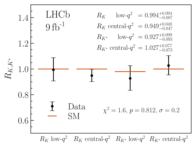
Figure 28: Measured values of LU observables in ${{B}^{+}}\!\rightarrow{{K}^{+}}{\ell^{+}}{\ell^{-}}$ and ${{B}^{0}}\!\rightarrow{{K}^{*0}}{\ell^{+}}{\ell^{-}}$ decays and their overall compatibility with the SM.

The results presented here differ from previous LHCb measurements of $R_{K}$ [24] and $R_{{{K}^{*}}}$ [21], which they supersede. The measured values for $R_{{{K}^{*}}}$ (low- and $\text{central-}{q^{2}}$) and $R_{K}$ ($\text{central-}{q^{2}}$) move upwards from the previous results and closer to the SM predictions. Although these shifts can be attributed in part to statistical effects it is understood that the change in $R_{K}$ is primarily due to systematic effects. In the case of $R_{K}$, the data sample is the same as in Ref. [24], but subject to a revised analysis. For $R_{K}$ ($\text{central-}{q^{2}}$) the statistical component of the difference is evaluated using pseudoexperiments and found to follow a Gaussian distribution of width 0.033 in the absolute value of $R_{K}$. In the case of $R_{{{K}^{*}}}$, the data correspond to more than a factor of five increase in the number of ${b}{\overline{b}}$ pairs produced relative to Ref. [21] and hence there is a much larger statistical component of the difference. For $R_{K}$ ($\text{central-}{q^{2}}$) the expected systematic shifts caused by the improved treatment of misidentified hadronic backgrounds in the electron mode are also evaluated using pseudoexperiments. The biggest shift (0.064 with respect to Ref. [24]) is found to be due to the more stringent PID criteria applied here, which reduce the contribution from misidentified background processes that had previously not been accounted for appropriately. In addition, the residual misidentified backgrounds are explicitly modeled in the fit, resulting in a further shift (0.038) compared to the previous analysis. These shifts add linearly. The systematic shift due to misidentified backgrounds to electrons, and the uncertainties assigned to the results presented here, are greater than the systematic uncertainties in the earlier publication of $R_{K}$. The assigned systematic uncertainties on the new measurements presented in this paper are smaller than in previous papers, except for $R_{K}$ ($\text{central-}{q^{2}}$) where the new result has a smaller overall relative uncertainty despite an increase in the systematic uncertainty from that of Ref. [24]. In all cases, the statistical uncertainties remain significantly larger than the systematic uncertainties and therefore additional data will continue to challenge the Standard Model.

LHCb collaboration

R. Aaij³² , A.S.W. Abdelmotteleb⁵⁰ , C. Abellan Beteta⁴⁴, F. Abudinén⁵⁰ , T. Ackernley⁵⁴ , B. Adeva⁴⁰ , M. Adinolfi⁴⁸ , P. Adlarson⁷⁷ , H. Afsharnia⁹, C. Agapopoulou¹³ , C.A. Aidala⁷⁸ , Z. Ajaltouni⁹, S. Akar⁵⁹ , K. Akiba³² , P. Albicocco²³ , J. Albrecht¹⁵ , F. Alessio⁴² , M. Alexander⁵³ , A. Alfonso Albero³⁹ , Z. Aliouche⁵⁶ , P. Alvarez Cartelle⁴⁹ , R. Amalric¹³ , S. Amato² , J.L. Amey⁴⁸ , Y. Amhis^11,42 , L. An⁴² , L. Anderlini²² , M. Andersson⁴⁴ , A. Andreianov³⁸ , M. Andreotti²¹ , D. Andreou⁶² , D. Ao⁶ , F. Archilli^31,t , A. Artamonov³⁸ , M. Artuso⁶² , E. Aslanides¹⁰ , M. Atzeni⁴⁴ , B. Audurier¹² , I. Bachiller Perea⁸ , S. Bachmann¹⁷ , M. Bachmayer⁴³ , J.J. Back⁵⁰ , A. Bailly-reyre¹³, P. Baladron Rodriguez⁴⁰ , V. Balagura¹² , W. Baldini^21,42 , J. Baptista de Souza Leite¹ , M. Barbetti^22,k , R.J. Barlow⁵⁶ , S. Barsuk¹¹ , W. Barter⁵² , M. Bartolini⁴⁹ , F. Baryshnikov³⁸ , J.M. Basels¹⁴ , G. Bassi^29,q , B. Batsukh⁴ , A. Battig¹⁵ , A. Bay⁴³ , A. Beck⁵⁰ , M. Becker¹⁵ , F. Bedeschi²⁹ , I.B. Bediaga¹ , A. Beiter⁶², S. Belin⁴⁰ , V. Bellee⁴⁴ , K. Belous³⁸ , I. Belov³⁸ , I. Belyaev³⁸ , G. Benane¹⁰ , G. Bencivenni²³ , E. Ben-Haim¹³ , A. Berezhnoy³⁸ , R. Bernet⁴⁴ , S. Bernet Andres⁷⁶ , D. Berninghoff¹⁷, H.C. Bernstein⁶², C. Bertella⁵⁶ , A. Bertolin²⁸ , C. Betancourt⁴⁴ , F. Betti⁴² , Ia. Bezshyiko⁴⁴ , J. Bhom³⁵ , L. Bian⁶⁸ , M.S. Bieker¹⁵ , N.V. Biesuz²¹ , S. Bifani⁴⁷ , P. Billoir¹³ , A. Biolchini³² , M. Birch⁵⁵ , F.C.R. Bishop⁴⁹ , A. Bitadze⁵⁶ , A. Bizzeti , M.P. Blago⁴⁹ , T. Blake⁵⁰ , F. Blanc⁴³ , J.E. Blank¹⁵ , S. Blusk⁶² , D. Bobulska⁵³ , J.A. Boelhauve¹⁵ , O. Boente Garcia¹² , T. Boettcher⁵⁹ , A. Boldyrev³⁸ , C.S. Bolognani⁷⁴ , R. Bolzonella^21,j , N. Bondar^38,42 , F. Borgato²⁸ , S. Borghi⁵⁶ , M. Borsato¹⁷ , J.T. Borsuk³⁵ , S.A. Bouchiba⁴³ , T.J.V. Bowcock⁵⁴ , A. Boyer⁴² , C. Bozzi²¹ , M.J. Bradley⁵⁵, S. Braun⁶⁰ , A. Brea Rodriguez⁴⁰ , J. Brodzicka³⁵ , A. Brossa Gonzalo⁴⁰ , J. Brown⁵⁴ , D. Brundu²⁷ , A. Buonaura⁴⁴ , L. Buonincontri²⁸ , A.T. Burke⁵⁶ , C. Burr⁴² , A. Bursche⁶⁶, A. Butkevich³⁸ , J.S. Butter³² , J. Buytaert⁴² , W. Byczynski⁴² , S. Cadeddu²⁷ , H. Cai⁶⁸, R. Calabrese^21,j , L. Calefice¹⁵ , S. Cali²³ , R. Calladine⁴⁷, M. Calvi^26,n , M. Calvo Gomez⁷⁶ , P. Campana²³ , D.H. Campora Perez⁷⁴ , A.F. Campoverde Quezada⁶ , S. Capelli^26,n , L. Capriotti²⁰ , A. Carbone^20,h , R. Cardinale^24,l , A. Cardini²⁷ , P. Carniti^26,n , L. Carus¹⁴, A. Casais Vidal⁴⁰ , R. Caspary¹⁷ , G. Casse⁵⁴ , M. Cattaneo⁴² , G. Cavallero^55,42 , V. Cavallini^21,j , S. Celani⁴³ , J. Cerasoli¹⁰ , D. Cervenkov⁵⁷ , A.J. Chadwick⁵⁴ , I. Chahrour⁷⁸ , M.G. Chapman⁴⁸, M. Charles¹³ , Ph. Charpentier⁴² , C.A. Chavez Barajas⁵⁴ , M. Chefdeville⁸ , C. Chen¹⁰ , S. Chen⁴ , A. Chernov³⁵ , S. Chernyshenko⁴⁶ , V. Chobanova⁴⁰ , S. Cholak⁴³ , M. Chrzaszcz³⁵ , A. Chubykin³⁸ , V. Chulikov³⁸ , P. Ciambrone²³ , M.F. Cicala⁵⁰ , X. Cid Vidal⁴⁰ , G. Ciezarek⁴² , P. Cifra⁴² , P.E.L. Clarke⁵² , M. Clemencic⁴² , H.V. Cliff⁴⁹ , J. Closier⁴² , J.L. Cobbledick⁵⁶ , V. Coco⁴² , J. Cogan¹⁰ , E. Cogneras⁹ , L. Cojocariu³⁷ , P. Collins⁴² , T. Colombo⁴² , L. Congedo¹⁹ , A. Contu²⁷ , N. Cooke⁴⁷ , I. Corredoira ⁴⁰ , G. Corti⁴² , B. Couturier⁴² , D.C. Craik⁴⁴ , M. Cruz Torres^1,f , R. Currie⁵² , C.L. Da Silva⁶¹ , S. Dadabaev³⁸ , L. Dai⁶⁵ , X. Dai⁵ , E. Dall’Occo¹⁵ , J. Dalseno⁴⁰ , C. D’Ambrosio⁴² , J. Daniel⁹ , A. Danilina³⁸ , P. d’Argent¹⁹ , J.E. Davies⁵⁶ , A. Davis⁵⁶ , O. De Aguiar Francisco⁵⁶ , J. de Boer⁴² , K. De Bruyn⁷³ , S. De Capua⁵⁶ , M. De Cian⁴³ , U. De Freitas Carneiro Da Graca¹ , E. De Lucia²³ , J.M. De Miranda¹ , L. De Paula² , M. De Serio^19,g , D. De Simone⁴⁴ , P. De Simone²³ , F. De Vellis¹⁵ , J.A. de Vries⁷⁴ , C.T. Dean⁶¹ , F. Debernardis^19,g , D. Decamp⁸ , V. Dedu¹⁰ , L. Del Buono¹³ , B. Delaney⁵⁸ , H.-P. Dembinski¹⁵ , V. Denysenko⁴⁴ , O. Deschamps⁹ , F. Desse¹¹, F. Dettori^27,i , B. Dey⁷¹ , P. Di Nezza²³ , I. Diachkov³⁸ , S. Didenko³⁸ , L. Dieste Maronas⁴⁰, S. Ding⁶² , V. Dobishuk⁴⁶ , A. Dolmatov³⁸, C. Dong³ , A.M. Donohoe¹⁸ , F. Dordei²⁷ , A.C. dos Reis¹ , L. Douglas⁵³, A.G. Downes⁸ , P. Duda⁷⁵ , M.W. Dudek³⁵ , L. Dufour⁴² , V. Duk⁷² , P. Durante⁴² , M. M. Duras⁷⁵ , J.M. Durham⁶¹ , D. Dutta⁵⁶ , A. Dziurda³⁵ , A. Dzyuba³⁸ , S. Easo⁵¹ , U. Egede⁶³ , V. Egorychev³⁸ , C. Eirea Orro⁴⁰, S. Eisenhardt⁵² , E. Ejopu⁵⁶ , S. Ek-In⁴³ , L. Eklund⁷⁷ , M. Elashri⁵⁹ , J. Ellbracht¹⁵ , S. Ely⁵⁵ , A. Ene³⁷ , E. Epple⁵⁹ , S. Escher¹⁴ , J. Eschle⁴⁴ , S. Esen⁴⁴ , T. Evans⁵⁶ , F. Fabiano^27,i , L.N. Falcao¹ , Y. Fan⁶ , B. Fang^11,68 , L. Fantini^72,p , M. Faria⁴³ , S. Farry⁵⁴ , D. Fazzini^26,n , L. Felkowski⁷⁵ , M. Feo⁴² , M. Fernandez Gomez⁴⁰ , A.D. Fernez⁶⁰ , F. Ferrari²⁰ , L. Ferreira Lopes⁴³ , F. Ferreira Rodrigues² , S. Ferreres Sole³² , M. Ferrillo⁴⁴ , M. Ferro-Luzzi⁴² , S. Filippov³⁸ , R.A. Fini¹⁹ , M. Fiorini^21,j , M. Firlej³⁴ , K.M. Fischer⁵⁷ , D.S. Fitzgerald⁷⁸ , C. Fitzpatrick⁵⁶ , T. Fiutowski³⁴ , F. Fleuret¹² , M. Fontana¹³ , F. Fontanelli^24,l , R. Forty⁴² , D. Foulds-Holt⁴⁹ , V. Franco Lima⁵⁴ , M. Franco Sevilla⁶⁰ , M. Frank⁴² , E. Franzoso^21,j , G. Frau¹⁷ , C. Frei⁴² , D.A. Friday⁵⁶ , L. Frontini^25,m , J. Fu⁶ , Q. Fuehring¹⁵ , T. Fulghesu¹³ , E. Gabriel³² , G. Galati^19,g , M.D. Galati³² , A. Gallas Torreira⁴⁰ , D. Galli^20,h , S. Gambetta^52,42 , M. Gandelman² , P. Gandini²⁵ , H. Gao⁶ , Y. Gao⁷ , Y. Gao⁵ , M. Garau^27,i , L.M. Garcia Martin⁵⁰ , P. Garcia Moreno³⁹ , J. García Pardiñas⁴² , B. Garcia Plana⁴⁰, F.A. Garcia Rosales¹² , L. Garrido³⁹ , C. Gaspar⁴² , R.E. Geertsema³² , D. Gerick¹⁷, L.L. Gerken¹⁵ , E. Gersabeck⁵⁶ , M. Gersabeck⁵⁶ , T. Gershon⁵⁰ , L. Giambastiani²⁸ , V. Gibson⁴⁹ , H.K. Giemza³⁶ , A.L. Gilman⁵⁷ , M. Giovannetti^23,t , A. Gioventù⁴⁰ , P. Gironella Gironell³⁹ , C. Giugliano^21,j , M.A. Giza³⁵ , K. Gizdov⁵² , E.L. Gkougkousis⁴² , V.V. Gligorov^13,42 , C. Göbel⁶⁴ , E. Golobardes⁷⁶ , D. Golubkov³⁸ , A. Golutvin^55,38 , A. Gomes^1,2,b,a,† , S. Gomez Fernandez³⁹ , F. Goncalves Abrantes⁵⁷ , M. Goncerz³⁵ , G. Gong³ , I.V. Gorelov³⁸ , C. Gotti²⁶ , J.P. Grabowski⁷⁰ , T. Grammatico¹³ , L.A. Granado Cardoso⁴² , E. Graugés³⁹ , E. Graverini⁴³ , G. Graziani , A. T. Grecu³⁷ , L.M. Greeven³² , N.A. Grieser⁵⁹ , L. Grillo⁵³ , S. Gromov³⁸ , B.R. Gruberg Cazon⁵⁷ , C.  Gu³ , M. Guarise^21,j , M. Guittiere¹¹ , P. A. Günther¹⁷ , E. Gushchin³⁸ , A. Guth¹⁴, Y. Guz^5,38 , T. Gys⁴² , T. Hadavizadeh⁶³ , C. Hadjivasiliou⁶⁰ , G. Haefeli⁴³ , C. Haen⁴² , J. Haimberger⁴² , S.C. Haines⁴⁹ , T. Halewood-leagas⁵⁴ , M.M. Halvorsen⁴² , P.M. Hamilton⁶⁰ , J. Hammerich⁵⁴ , Q. Han⁷ , X. Han¹⁷ , S. Hansmann-Menzemer¹⁷ , L. Hao⁶ , N. Harnew⁵⁷ , T. Harrison⁵⁴ , C. Hasse⁴² , M. Hatch⁴² , J. He^6,d , K. Heijhoff³² , F. Hemmer⁴² , C. Henderson⁵⁹ , R.D.L. Henderson^63,50 , A.M. Hennequin⁵⁸ , K. Hennessy⁵⁴ , L. Henry⁴² , J. Herd⁵⁵ , J. Heuel¹⁴ , A. Hicheur² , D. Hill⁴³ , M. Hilton⁵⁶ , S.E. Hollitt¹⁵ , J. Horswill⁵⁶ , R. Hou⁷ , Y. Hou⁸ , J. Hu¹⁷, J. Hu⁶⁶ , W. Hu⁵ , X. Hu³ , W. Huang⁶ , X. Huang⁶⁸, W. Hulsbergen³² , R.J. Hunter⁵⁰ , M. Hushchyn³⁸ , D. Hutchcroft⁵⁴ , P. Ibis¹⁵ , M. Idzik³⁴ , D. Ilin³⁸ , P. Ilten⁵⁹ , A. Inglessi³⁸ , A. Iniukhin³⁸ , A. Ishteev³⁸ , K. Ivshin³⁸ , R. Jacobsson⁴² , H. Jage¹⁴ , S.J. Jaimes Elles⁴¹ , S. Jakobsen⁴² , E. Jans³² , B.K. Jashal⁴¹ , A. Jawahery⁶⁰ , V. Jevtic¹⁵ , E. Jiang⁶⁰ , X. Jiang^4,6 , Y. Jiang⁶ , M. John⁵⁷ , D. Johnson⁵⁸ , C.R. Jones⁴⁹ , T.P. Jones⁵⁰ , S. Joshi³⁶ , B. Jost⁴² , N. Jurik⁴² , I. Juszczak³⁵ , S. Kandybei⁴⁵ , Y. Kang³ , M. Karacson⁴² , D. Karpenkov³⁸ , M. Karpov³⁸ , J.W. Kautz⁵⁹ , F. Keizer⁴² , D.M. Keller⁶² , M. Kenzie⁵⁰ , T. Ketel³² , B. Khanji¹⁵ , A. Kharisova³⁸ , S. Kholodenko³⁸ , G. Khreich¹¹ , T. Kirn¹⁴ , V.S. Kirsebom⁴³ , O. Kitouni⁵⁸ , S. Klaver³³ , N. Kleijne^29,q , K. Klimaszewski³⁶ , M.R. Kmiec³⁶ , S. Koliiev⁴⁶ , L. Kolk¹⁵ , A. Kondybayeva³⁸ , A. Konoplyannikov³⁸ , P. Kopciewicz³⁴ , R. Kopecna¹⁷, P. Koppenburg³² , M. Korolev³⁸ , I. Kostiuk³² , O. Kot⁴⁶, S. Kotriakhova , A. Kozachuk³⁸ , P. Kravchenko³⁸ , L. Kravchuk³⁸ , R.D. Krawczyk⁴² , M. Kreps⁵⁰ , S. Kretzschmar¹⁴ , P. Krokovny³⁸ , W. Krupa³⁴ , W. Krzemien³⁶ , J. Kubat¹⁷, S. Kubis⁷⁵ , W. Kucewicz³⁵ , M. Kucharczyk³⁵ , V. Kudryavtsev³⁸ , E. Kulikova³⁸ , A. Kupsc⁷⁷ , D. Lacarrere⁴² , G. Lafferty⁵⁶ , A. Lai²⁷ , A. Lampis^27,i , D. Lancierini⁴⁴ , C. Landesa Gomez⁴⁰ , J.J. Lane⁵⁶ , R. Lane⁴⁸ , C. Langenbruch¹⁴ , J. Langer¹⁵ , O. Lantwin³⁸ , T. Latham⁵⁰ , F. Lazzari^29,r , M. Lazzaroni^25,m , C. Lazzeroni⁴⁷ , R. Le Gac¹⁰ , S.H. Lee⁷⁸ , R. Lefèvre⁹ , A. Leflat³⁸ , S. Legotin³⁸ , C. Lemettais⁴³ , O. Leroy¹⁰ , T. Lesiak³⁵ , B. Leverington¹⁷ , A. Li³ , H. Li⁶⁶ , K. Li⁷ , P. Li⁴² , P.-R. Li⁶⁷ , S. Li⁷ , T. Li⁴ , T. Li⁶⁶ , Y. Li⁴ , Z. Li⁶² , X. Liang⁶² , C. Lin⁶ , T. Lin⁵¹ , R. Lindner⁴² , V. Lisovskyi¹⁵ , R. Litvinov^27,i , G. Liu⁶⁶ , H. Liu⁶ , K. Liu⁶⁷ , Q. Liu⁶ , S. Liu^4,6 , A. Lobo Salvia³⁹ , A. Loi²⁷ , R. Lollini⁷² , J. Lomba Castro⁴⁰ , I. Longstaff⁵³, J.H. Lopes² , A. Lopez Huertas³⁹ , S. López Soliño⁴⁰ , G.H. Lovell⁴⁹ , Y. Lu^4,c , C. Lucarelli^22,k , D. Lucchesi^28,o , S. Luchuk³⁸ , M. Lucio Martinez⁷⁴ , V. Lukashenko^32,46 , Y. Luo³ , A. Lupato⁵⁶ , E. Luppi^21,j , A. Lusiani^29,q , K. Lynch¹⁸ , X.-R. Lyu⁶ , R. Ma⁶ , S. Maccolini¹⁵ , F. Machefert¹¹ , F. Maciuc³⁷ , I. Mackay⁵⁷ , V. Macko⁴³ , L.R. Madhan Mohan⁴⁹ , A. Maevskiy³⁸ , D. Maisuzenko³⁸ , M.W. Majewski³⁴, J.J. Malczewski³⁵ , S. Malde⁵⁷ , B. Malecki^35,42 , A. Malinin³⁸ , T. Maltsev³⁸ , G. Manca^27,i , G. Mancinelli¹⁰ , C. Mancuso^11,25,m , R. Manera Escalero³⁹, D. Manuzzi²⁰ , C.A. Manzari⁴⁴ , D. Marangotto^25,m , J.F. Marchand⁸ , U. Marconi²⁰ , S. Mariani^22,k , C. Marin Benito³⁹ , J. Marks¹⁷ , A.M. Marshall⁴⁸ , P.J. Marshall⁵⁴, G. Martelli^72,p , G. Martellotti³⁰ , L. Martinazzoli^42,n , M. Martinelli^26,n , D. Martinez Santos⁴⁰ , F. Martinez Vidal⁴¹ , A. Massafferri¹ , M. Materok¹⁴ , R. Matev⁴² , A. Mathad⁴⁴ , V. Matiunin³⁸ , C. Matteuzzi²⁶ , K.R. Mattioli¹² , A. Mauri⁵⁵ , E. Maurice¹² , J. Mauricio³⁹ , M. Mazurek⁴² , M. McCann⁵⁵ , L. Mcconnell¹⁸ , T.H. McGrath⁵⁶ , N.T. McHugh⁵³ , A. McNab⁵⁶ , R. McNulty¹⁸ , B. Meadows⁵⁹ , G. Meier¹⁵ , D. Melnychuk³⁶ , S. Meloni^26,n , M. Merk^32,74 , A. Merli^25,m , L. Meyer Garcia² , D. Miao^4,6 , M. Mikhasenko^70,e , D.A. Milanes⁶⁹ , E. Millard⁵⁰, M. Milovanovic⁴² , M.-N. Minard^8,†, A. Minotti^26,n , T. Miralles⁹ , S.E. Mitchell⁵² , B. Mitreska¹⁵ , D.S. Mitzel¹⁵ , A. Modak⁵¹ , A. Mödden ¹⁵ , R.A. Mohammed⁵⁷ , R.D. Moise¹⁴ , S. Mokhnenko³⁸ , T. Mombächer⁴⁰ , M. Monk^50,63 , I.A. Monroy⁶⁹ , S. Monteil⁹ , G. Morello²³ , M.J. Morello^29,q , M.P. Morgenthaler¹⁷ , J. Moron³⁴ , A.B. Morris⁴² , A.G. Morris⁵⁰ , R. Mountain⁶² , H. Mu³ , E. Muhammad⁵⁰ , F. Muheim⁵² , M. Mulder⁷³ , K. Müller⁴⁴ , C.H. Murphy⁵⁷ , D. Murray⁵⁶ , R. Murta⁵⁵ , P. Muzzetto^27,i , P. Naik⁴⁸ , T. Nakada⁴³ , R. Nandakumar⁵¹ , T. Nanut⁴² , I. Nasteva² , M. Needham⁵² , N. Neri^25,m , S. Neubert⁷⁰ , N. Neufeld⁴² , P. Neustroev³⁸, R. Newcombe⁵⁵, J. Nicolini^15,11 , D. Nicotra⁷⁴ , E.M. Niel⁴³ , S. Nieswand¹⁴, N. Nikitin³⁸ , N.S. Nolte⁵⁸ , C. Normand^8,i,27 , J. Novoa Fernandez⁴⁰ , G. Nowak⁵⁹ , C. Nunez⁷⁸ , A. Oblakowska-Mucha³⁴ , V. Obraztsov³⁸ , T. Oeser¹⁴ , S. Okamura^21,j , R. Oldeman^27,i , F. Oliva⁵² , C.J.G. Onderwater⁷³ , R.H. O’Neil⁵² , J.M. Otalora Goicochea² , T. Ovsiannikova³⁸ , P. Owen⁴⁴ , A. Oyanguren⁴¹ , O. Ozcelik⁵² , K.O. Padeken⁷⁰ , B. Pagare⁵⁰ , P.R. Pais⁴² , T. Pajero⁵⁷ , A. Palano¹⁹ , M. Palutan²³ , G. Panshin³⁸ , L. Paolucci⁵⁰ , A. Papanestis⁵¹ , M. Pappagallo^19,g , L.L. Pappalardo^21,j , C. Pappenheimer⁵⁹ , W. Parker⁶⁰ , C. Parkes^56,42 , B. Passalacqua^21,j , G. Passaleva²² , A. Pastore¹⁹ , M. Patel⁵⁵ , C. Patrignani^20,h , C.J. Pawley⁷⁴ , A. Pellegrino³² , M. Pepe Altarelli⁴² , S. Perazzini²⁰ , D. Pereima³⁸ , A. Pereiro Castro⁴⁰ , P. Perret⁹ , K. Petridis⁴⁸ , A. Petrolini^24,l , S. Petrucci⁵² , M. Petruzzo²⁵ , H. Pham⁶² , A. Philippov³⁸ , R. Piandani⁶ , L. Pica^29,q , M. Piccini⁷² , B. Pietrzyk⁸ , G. Pietrzyk¹¹ , M. Pili⁵⁷ , D. Pinci³⁰ , F. Pisani⁴² , M. Pizzichemi^26,n,42 , V. Placinta³⁷ , J. Plews⁴⁷ , M. Plo Casasus⁴⁰ , F. Polci^13,42 , M. Poli Lener²³ , A. Poluektov¹⁰ , N. Polukhina³⁸ , I. Polyakov⁴² , E. Polycarpo² , S. Ponce⁴² , D. Popov^6,42 , S. Poslavskii³⁸ , K. Prasanth³⁵ , L. Promberger¹⁷ , C. Prouve⁴⁰ , V. Pugatch⁴⁶ , V. Puill¹¹ , G. Punzi^29,r , H.R. Qi³ , W. Qian⁶ , N. Qin³ , S. Qu³ , R. Quagliani⁴³ , N.V. Raab¹⁸ , B. Rachwal³⁴ , J.H. Rademacker⁴⁸ , R. Rajagopalan⁶², M. Rama²⁹ , M. Ramos Pernas⁵⁰ , M.S. Rangel² , F. Ratnikov³⁸ , G. Raven³³ , M. Rebollo De Miguel⁴¹ , F. Redi⁴² , J. Reich⁴⁸ , F. Reiss⁵⁶ , C. Remon Alepuz⁴¹, Z. Ren³ , P.K. Resmi⁵⁷ , R. Ribatti^29,q , A.M. Ricci²⁷ , S. Ricciardi⁵¹ , K. Richardson⁵⁸ , M. Richardson-Slipper⁵² , K. Rinnert⁵⁴ , P. Robbe¹¹ , G. Robertson⁵² , E. Rodrigues^54,42 , E. Rodriguez Fernandez⁴⁰ , J.A. Rodriguez Lopez⁶⁹ , E. Rodriguez Rodriguez⁴⁰ , D.L. Rolf⁴² , A. Rollings⁵⁷ , P. Roloff⁴² , V. Romanovskiy³⁸ , M. Romero Lamas⁴⁰ , A. Romero Vidal⁴⁰ , J.D. Roth^78,†, M. Rotondo²³ , M.S. Rudolph⁶² , T. Ruf⁴² , R.A. Ruiz Fernandez⁴⁰ , J. Ruiz Vidal⁴¹ , A. Ryzhikov³⁸ , J. Ryzka³⁴ , J.J. Saborido Silva⁴⁰ , N. Sagidova³⁸ , N. Sahoo⁴⁷ , B. Saitta^27,i , M. Salomoni⁴² , C. Sanchez Gras³² , I. Sanderswood⁴¹ , R. Santacesaria³⁰ , C. Santamarina Rios⁴⁰ , M. Santimaria²³ , E. Santovetti^31,t , D. Saranin³⁸ , G. Sarpis¹⁴ , M. Sarpis⁷⁰ , A. Sarti³⁰ , C. Satriano^30,s , A. Satta³¹ , M. Saur¹⁵ , D. Savrina³⁸ , H. Sazak⁹ , L.G. Scantlebury Smead⁵⁷ , A. Scarabotto¹³ , S. Schael¹⁴ , S. Scherl⁵⁴ , M. Schiller⁵³ , H. Schindler⁴² , M. Schmelling¹⁶ , B. Schmidt⁴² , S. Schmitt¹⁴ , O. Schneider⁴³ , A. Schopper⁴² , M. Schubiger³² , S. Schulte⁴³ , M.H. Schune¹¹ , R. Schwemmer⁴² , B. Sciascia²³ , A. Sciuccati⁴² , S. Sellam⁴⁰ , A. Semennikov³⁸ , M. Senghi Soares³³ , A. Sergi^24,l , N. Serra⁴⁴ , L. Sestini²⁸ , A. Seuthe¹⁵ , Y. Shang⁵ , D.M. Shangase⁷⁸ , M. Shapkin³⁸ , I. Shchemerov³⁸ , L. Shchutska⁴³ , T. Shears⁵⁴ , L. Shekhtman³⁸ , Z. Shen⁵ , S. Sheng^4,6 , V. Shevchenko³⁸ , B. Shi⁶ , E.B. Shields^26,n , Y. Shimizu¹¹ , E. Shmanin³⁸ , R. Shorkin³⁸ , J.D. Shupperd⁶² , B.G. Siddi^21,j , R. Silva Coutinho⁶² , G. Simi²⁸ , S. Simone^19,g , M. Singla⁶³ , N. Skidmore⁵⁶ , R. Skuza¹⁷ , T. Skwarnicki⁶² , M.W. Slater⁴⁷ , J.C. Smallwood⁵⁷ , J.G. Smeaton⁴⁹ , E. Smith⁴⁴ , K. Smith⁶¹ , M. Smith⁵⁵ , A. Snoch³² , L. Soares Lavra⁹ , M.D. Sokoloff⁵⁹ , F.J.P. Soler⁵³ , A. Solomin^38,48 , A. Solovev³⁸ , I. Solovyev³⁸ , R. Song⁶³ , F.L. Souza De Almeida² , B. Souza De Paula² , B. Spaan^15,†, E. Spadaro Norella^25,m , E. Spedicato²⁰ , E. Spiridenkov³⁸, P. Spradlin⁵³ , V. Sriskaran⁴² , F. Stagni⁴² , M. Stahl⁴² , S. Stahl⁴² , S. Stanislaus⁵⁷ , E.N. Stein⁴² , O. Steinkamp⁴⁴ , O. Stenyakin³⁸, H. Stevens¹⁵ , S. Stone^62,42,† , D. Strekalina³⁸ , Y. Su⁶ , F. Suljik⁵⁷ , J. Sun²⁷ , L. Sun⁶⁸ , Y. Sun⁶⁰ , P.N. Swallow⁴⁷ , K. Swientek³⁴ , A. Szabelski³⁶ , T. Szumlak³⁴ , M. Szymanski⁴² , Y. Tan³ , S. Taneja⁵⁶ , M.D. Tat⁵⁷ , A. Terentev⁴⁴ , F. Teubert⁴² , E. Thomas⁴² , D.J.D. Thompson⁴⁷ , K.A. Thomson⁵⁴ , H. Tilquin⁵⁵ , V. Tisserand⁹ , S. T’Jampens⁸ , M. Tobin⁴ , L. Tomassetti^21,j , G. Tonani^25,m , X. Tong⁵ , D. Torres Machado¹ , D.Y. Tou³ , C. Trippl⁴³ , G. Tuci⁶ , N. Tuning³² , A. Ukleja³⁶ , D.J. Unverzagt¹⁷ , A. Usachov³³ , A. Ustyuzhanin³⁸ , U. Uwer¹⁷ , A. Vagner³⁸, V. Vagnoni²⁰ , A. Valassi⁴² , G. Valenti²⁰ , N. Valls Canudas⁷⁶ , M. Van Dijk⁴³ , H. Van Hecke⁶¹ , E. van Herwijnen⁵⁵ , C.B. Van Hulse^40,v , M. van Veghel³² , R. Vazquez Gomez³⁹ , P. Vazquez Regueiro⁴⁰ , C. Vázquez Sierra⁴² , S. Vecchi²¹ , J.J. Velthuis⁴⁸ , M. Veltri^22,u , A. Venkateswaran⁴³ , M. Veronesi³² , M. Vesterinen⁵⁰ , D.  Vieira⁵⁹ , M. Vieites Diaz⁴³ , X. Vilasis-Cardona⁷⁶ , E. Vilella Figueras⁵⁴ , A. Villa²⁰ , P. Vincent¹³ , F.C. Volle¹¹ , D. vom Bruch¹⁰ , A. Vorobyev³⁸, V. Vorobyev³⁸, N. Voropaev³⁸ , K. Vos⁷⁴ , C. Vrahas⁵² , J. Walsh²⁹ , E.J. Walton⁶³ , G. Wan⁵ , C. Wang¹⁷ , G. Wang⁷ , J. Wang⁵ , J. Wang⁴ , J. Wang³ , J. Wang⁶⁸ , M. Wang²⁵ , R. Wang⁴⁸ , X. Wang⁶⁶ , Y. Wang⁷ , Z. Wang⁴⁴ , Z. Wang³ , Z. Wang⁶ , J.A. Ward^50,63 , N.K. Watson⁴⁷ , D. Websdale⁵⁵ , Y. Wei⁵ , B.D.C. Westhenry⁴⁸ , D.J. White⁵⁶ , M. Whitehead⁵³ , A.R. Wiederhold⁵⁰ , D. Wiedner¹⁵ , G. Wilkinson⁵⁷ , M.K. Wilkinson⁵⁹ , I. Williams⁴⁹, M. Williams⁵⁸ , M.R.J. Williams⁵² , R. Williams⁴⁹ , F.F. Wilson⁵¹ , W. Wislicki³⁶ , M. Witek³⁵ , L. Witola¹⁷ , C.P. Wong⁶¹ , G. Wormser¹¹ , S.A. Wotton⁴⁹ , H. Wu⁶² , J. Wu⁷ , K. Wyllie⁴² , Z. Xiang⁶ , Y. Xie⁷ , A. Xu⁵ , J. Xu⁶ , L. Xu³ , L. Xu³ , M. Xu⁵⁰ , Q. Xu⁶, Z. Xu⁹ , Z. Xu⁶ , D. Yang³ , S. Yang⁶ , X. Yang⁵ , Y. Yang⁶ , Z. Yang⁵ , Z. Yang⁶⁰ , L.E. Yeomans⁵⁴ , V. Yeroshenko¹¹ , H. Yeung⁵⁶ , H. Yin⁷ , J. Yu⁶⁵ , X. Yuan⁶² , E. Zaffaroni⁴³ , M. Zavertyaev¹⁶ , M. Zdybal³⁵ , M. Zeng³ , C. Zhang⁵ , D. Zhang⁷ , L. Zhang³ , S. Zhang⁶⁵ , S. Zhang⁵ , Y. Zhang⁵ , Y. Zhang⁵⁷, Y. Zhao¹⁷ , A. Zharkova³⁸ , A. Zhelezov¹⁷ , Y. Zheng⁶ , T. Zhou⁵ , X. Zhou⁷ , Y. Zhou⁶ , V. Zhovkovska¹¹ , X. Zhu³ , X. Zhu⁷ , Z. Zhu⁶ , V. Zhukov^14,38 , Q. Zou^4,6 , S. Zucchelli^20,h , D. Zuliani²⁸ , G. Zunica⁵⁶ .

¹Centro Brasileiro de Pesquisas Físicas (CBPF), Rio de Janeiro, Brazil
²Universidade Federal do Rio de Janeiro (UFRJ), Rio de Janeiro, Brazil
³Center for High Energy Physics, Tsinghua University, Beijing, China
⁴Institute Of High Energy Physics (IHEP), Beijing, China
⁵School of Physics State Key Laboratory of Nuclear Physics and Technology, Peking University, Beijing, China
⁶University of Chinese Academy of Sciences, Beijing, China
⁷Institute of Particle Physics, Central China Normal University, Wuhan, Hubei, China
⁸Université Savoie Mont Blanc, CNRS, IN2P3-LAPP, Annecy, France
⁹Université Clermont Auvergne, CNRS/IN2P3, LPC, Clermont-Ferrand, France
¹⁰Aix Marseille Univ, CNRS/IN2P3, CPPM, Marseille, France
¹¹Université Paris-Saclay, CNRS/IN2P3, IJCLab, Orsay, France
¹²Laboratoire Leprince-Ringuet, CNRS/IN2P3, Ecole Polytechnique, Institut Polytechnique de Paris, Palaiseau, France
¹³LPNHE, Sorbonne Université, Paris Diderot Sorbonne Paris Cité, CNRS/IN2P3, Paris, France
¹⁴I. Physikalisches Institut, RWTH Aachen University, Aachen, Germany
¹⁵Fakultät Physik, Technische Universität Dortmund, Dortmund, Germany
¹⁶Max-Planck-Institut für Kernphysik (MPIK), Heidelberg, Germany
¹⁷Physikalisches Institut, Ruprecht-Karls-Universität Heidelberg, Heidelberg, Germany
¹⁸School of Physics, University College Dublin, Dublin, Ireland
¹⁹INFN Sezione di Bari, Bari, Italy
²⁰INFN Sezione di Bologna, Bologna, Italy
²¹INFN Sezione di Ferrara, Ferrara, Italy
²²INFN Sezione di Firenze, Firenze, Italy
²³INFN Laboratori Nazionali di Frascati, Frascati, Italy
²⁴INFN Sezione di Genova, Genova, Italy
²⁵INFN Sezione di Milano, Milano, Italy
²⁶INFN Sezione di Milano-Bicocca, Milano, Italy
²⁷INFN Sezione di Cagliari, Monserrato, Italy
²⁸Università degli Studi di Padova, Università e INFN, Padova, Padova, Italy
²⁹INFN Sezione di Pisa, Pisa, Italy
³⁰INFN Sezione di Roma La Sapienza, Roma, Italy
³¹INFN Sezione di Roma Tor Vergata, Roma, Italy
³²Nikhef National Institute for Subatomic Physics, Amsterdam, Netherlands
³³Nikhef National Institute for Subatomic Physics and VU University Amsterdam, Amsterdam, Netherlands
³⁴AGH - University of Science and Technology, Faculty of Physics and Applied Computer Science, Kraków, Poland
³⁵Henryk Niewodniczanski Institute of Nuclear Physics Polish Academy of Sciences, Kraków, Poland
³⁶National Center for Nuclear Research (NCBJ), Warsaw, Poland
³⁷Horia Hulubei National Institute of Physics and Nuclear Engineering, Bucharest-Magurele, Romania
³⁸Affiliated with an institute covered by a cooperation agreement with CERN
³⁹ICCUB, Universitat de Barcelona, Barcelona, Spain
⁴⁰Instituto Galego de Física de Altas Enerxías (IGFAE), Universidade de Santiago de Compostela, Santiago de Compostela, Spain
⁴¹Instituto de Fisica Corpuscular, Centro Mixto Universidad de Valencia - CSIC, Valencia, Spain
⁴²European Organization for Nuclear Research (CERN), Geneva, Switzerland
⁴³Institute of Physics, Ecole Polytechnique Fédérale de Lausanne (EPFL), Lausanne, Switzerland
⁴⁴Physik-Institut, Universität Zürich, Zürich, Switzerland
⁴⁵NSC Kharkiv Institute of Physics and Technology (NSC KIPT), Kharkiv, Ukraine
⁴⁶Institute for Nuclear Research of the National Academy of Sciences (KINR), Kyiv, Ukraine
⁴⁷University of Birmingham, Birmingham, United Kingdom
⁴⁸H.H. Wills Physics Laboratory, University of Bristol, Bristol, United Kingdom
⁴⁹Cavendish Laboratory, University of Cambridge, Cambridge, United Kingdom
⁵⁰Department of Physics, University of Warwick, Coventry, United Kingdom
⁵¹STFC Rutherford Appleton Laboratory, Didcot, United Kingdom
⁵²School of Physics and Astronomy, University of Edinburgh, Edinburgh, United Kingdom
⁵³School of Physics and Astronomy, University of Glasgow, Glasgow, United Kingdom
⁵⁴Oliver Lodge Laboratory, University of Liverpool, Liverpool, United Kingdom
⁵⁵Imperial College London, London, United Kingdom
⁵⁶Department of Physics and Astronomy, University of Manchester, Manchester, United Kingdom
⁵⁷Department of Physics, University of Oxford, Oxford, United Kingdom
⁵⁸Massachusetts Institute of Technology, Cambridge, MA, United States
⁵⁹University of Cincinnati, Cincinnati, OH, United States
⁶⁰University of Maryland, College Park, MD, United States
⁶¹Los Alamos National Laboratory (LANL), Los Alamos, NM, United States
⁶²Syracuse University, Syracuse, NY, United States
⁶³School of Physics and Astronomy, Monash University, Melbourne, Australia, associated to ^50
64Pontifícia Universidade Católica do Rio de Janeiro (PUC-Rio), Rio de Janeiro, Brazil, associated to ^2
65School of Physics and Electronics, Hunan University, Changsha City, China, associated to ^7
66Guangdong Provincial Key Laboratory of Nuclear Science, Guangdong-Hong Kong Joint Laboratory of Quantum Matter, Institute of Quantum Matter, South China Normal University, Guangzhou, China, associated to ^3
67Lanzhou University, Lanzhou, China, associated to ^4
68School of Physics and Technology, Wuhan University, Wuhan, China, associated to ^3
69Departamento de Fisica , Universidad Nacional de Colombia, Bogota, Colombia, associated to ^13
70Universität Bonn - Helmholtz-Institut für Strahlen und Kernphysik, Bonn, Germany, associated to ^17
71Eotvos Lorand University, Budapest, Hungary, associated to ^42
72INFN Sezione di Perugia, Perugia, Italy, associated to ^21
73Van Swinderen Institute, University of Groningen, Groningen, Netherlands, associated to ^32
74Universiteit Maastricht, Maastricht, Netherlands, associated to ^32
75Tadeusz Kosciuszko Cracow University of Technology, Cracow, Poland, associated to ^35
76DS4DS, La Salle, Universitat Ramon Llull, Barcelona, Spain, associated to ^39
77Department of Physics and Astronomy, Uppsala University, Uppsala, Sweden, associated to ^53
78University of Michigan, Ann Arbor, MI, United States, associated to <sup>62

a</sup>Universidade de Brasília, Brasília, Brazil
^bUniversidade Federal do Triângulo Mineiro (UFTM), Uberaba-MG, Brazil
^cCentral South U., Changsha, China
^dHangzhou Institute for Advanced Study, UCAS, Hangzhou, China
^eExcellence Cluster ORIGINS, Munich, Germany
^fUniversidad Nacional Autónoma de Honduras, Tegucigalpa, Honduras
^gUniversità di Bari, Bari, Italy
^hUniversità di Bologna, Bologna, Italy
ⁱUniversità di Cagliari, Cagliari, Italy
^jUniversità di Ferrara, Ferrara, Italy
^kUniversità di Firenze, Firenze, Italy
^lUniversità di Genova, Genova, Italy
^mUniversità degli Studi di Milano, Milano, Italy
ⁿUniversità di Milano Bicocca, Milano, Italy
^oUniversità di Padova, Padova, Italy
^pUniversità di Perugia, Perugia, Italy
^qScuola Normale Superiore, Pisa, Italy
^rUniversità di Pisa, Pisa, Italy
^sUniversità della Basilicata, Potenza, Italy
^tUniversità di Roma Tor Vergata, Roma, Italy
^uUniversità di Urbino, Urbino, Italy
^vUniversidad de Alcalá, Alcalá de Henares , Spain
^†Deceased

Appendix A Results split by data-taking period

The results obtained using the Run 1, Run 2p1, Run 2p2 datasets alone for $R_{K}$ and $R_{{{K}^{*}}}$ in the low- and $\text{central-}{q^{2}}$ regions are shown together with their likelihood profiles including all systematic uncertainties. The results obtained from the best fit in individual run periods are shown in Table 12 and the corresponding one-dimensional likelihood scans are shown in Fig. 29.

Table 12: Measured values of the LU observables obtained from the separate run periods. Uncertainties are split into statistical and systematic components and have been extracted from the one-dimensional likelihood scans.

LU observable	Run 1	Run 2p1	Run 2p2
$R_{K}$ $\text{low-}{q^{2}}$	$1.027\,^{\,+\,0.243\,+\,0.092}_{\,-\,0.180\,-\,0.073}$	$1.039\,^{\,+\,0.203\,+\,0.027}_{\,-\,0.149\,-\,0.027}$	$0.953\,^{\,+\,0.123\,+\,0.029}_{\,-\,0.104\,-\,0.026}$
$R_{{{K}^{*}}}$ $\text{low-}{q^{2}}$	$1.212\,^{\,+\,0.344\,+\,0.149}_{\,-\,0.240\,-\,0.114}$	$1.021\,^{\,+\,0.234\,+\,0.036}_{\,-\,0.187\,-\,0.027}$	$0.825\,^{\,+\,0.108\,+\,0.036}_{\,-\,0.091\,-\,0.031}$
$R_{K}$ $\text{central-}{q^{2}}$	$0.839\,^{\,+\,0.083\,+\,0.062}_{\,-\,0.073\,-\,0.056}$	$0.929\,^{\,+\,0.082\,+\,0.023}_{\,-\,0.073\,-\,0.020}$	$1.001\,^{\,+\,0.066\,+\,0.024}_{\,-\,0.061\,-\,0.022}$
$R_{{{K}^{*}}}$ $\text{central-}{q^{2}}$	$1.082\,^{\,+\,0.214\,+\,0.176}_{\,-\,0.165\,-\,0.148}$	$1.154\,^{\,+\,0.179\,+\,0.027}_{\,-\,0.147\,-\,0.023}$	$0.962\,^{\,+\,0.091\,+\,0.020}_{\,-\,0.080\,-\,0.018}$

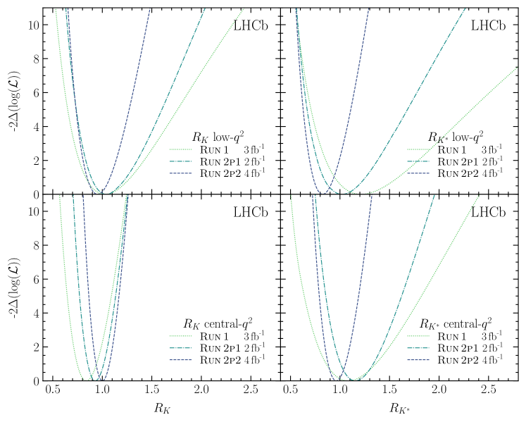
Figure 29: One-dimensional likelihood scans for $R_{K}$ and $R_{{{K}^{*}}}$ in the low- and $\text{central-}{q^{2}}$ regions, performing the measurements in each data-taking period separately. The scan shown includes both systematic and statistical uncertainties.

References

- [1] UA1 collaboration, C. Albajar et al., Studies of intermediate vector boson production and decay in UA1 at the CERN Proton-Antiproton Collider, Z. Phys. C44 (1989) 15
- [2] CDF collaboration, F. Abe et al., Measurement of the ratio , in collisions at TeV, Phys. Rev. Lett. 68 (1992) 3398
- [3] UA2 collaboration, J. Alitti et al., A search for charged Higgs from top quark decay at the CERN collider, Phys. Lett. B280 (1992) 137
- [4] CDF collaboration, F. Abe et al., A measurement of the production and muonic decay rate of and bosons in collisions at TeV, Phys. Rev. Lett. 69 (1992) 28
- [5] D0 collaboration, S. Abachi et al., and boson production in collisions at = 1.8 TeV, Phys. Rev. Lett. 75 (1995) 1456, arXiv:hep-ex/9505013
- [6] D0 collaboration, B. Abbott et al., A measurement of the production cross-section in collisions at TeV, Phys. Rev. Lett. 84 (2000) 5710, arXiv:hep-ex/9912065
- [7] ALEPH, DELPHI, L3, OPAL, SLD, LEP Electroweak Working Group, SLD Electroweak Group, SLD Heavy Flavour Group, S. Schael et al., Precision electroweak measurements on the resonance, Phys. Rept. 427 (2006) 257, arXiv:hep-ex/0509008
- [8] ALEPH, DELPHI, L3, OPAL, LEP Electroweak collaboration, S. Schael et al., Electroweak measurements in electron-positron collisions at W-boson-pair energies at LEP, Phys. Rept. 532 (2013) 119, arXiv:1302.3415
- [9] ATLAS collaboration, M. Aaboud et al., Precision measurement and interpretation of inclusive , and production cross sections with the ATLAS detector, Eur. Phys. J. C77 (2017) 367, arXiv:1612.03016
- [10] LHCb collaboration, R. Aaij et al., Measurement of forward production in collisions at 8 TeV, JHEP 10 (2016) 030, arXiv:1608.01484
- [11] LHCb collaboration, R. Aaij et al., Measurement of production in proton-proton collisions at 8 TeV, JHEP 09 (2018) 159, arXiv:1806.05008
- [12] CMS collaboration, A. Tumasyan et al., Search for new particles in events with energetic jets and large missing transverse momentum in proton-proton collisions at = 13 TeV, JHEP 11 (2021) 153, arXiv:2107.13021
- [13] ATLAS collaboration, G. Aad et al., Search for new phenomena in collisions in final states with tau leptons, b-jets, and missing transverse momentum with the ATLAS detector, Phys. Rev. D104 (2021) 112005, arXiv:2108.07665
- [14] M. Bordone, G. Isidori, and A. Pattori, On the Standard Model predictions for and , Eur. Phys. J. C76 (2016) 440, arXiv:1605.07633
- [15] G. Isidori, S. Nabeebaccus, and R. Zwicky, QED corrections in at the double-differential level, JHEP 12 (2020) 104, arXiv:2009.00929
- [16] G. Isidori, D. Lancierini, S. Nabeebaccus, and R. Zwicky, QED in LFU ratios: theory versus experiment, a Monte Carlo study, JHEP 10 (2022) 146, arXiv:2205.08635
- [17] LHCb collaboration, Physics case for an LHCb Upgrade II — Opportunities in flavour physics, and beyond, in the HL-LHC era, arXiv:1808.08865
- [18] Y. Wang and D. Atwood, Rate difference between and in supersymmetry with large tan , Phys. Rev. D68 (2003) 094016, arXiv:hep-ph/0304248
- [19] G. Hiller and F. Krüger, More model-independent analysis of processes, Phys. Rev. D69 (2004) 074020, arXiv:hep-ph/0310219
- [20] LHCb collaboration, R. Aaij et al., Test of lepton universality using decays, Phys. Rev. Lett. 113 (2014) 151601, arXiv:1406.6482
- [21] LHCb collaboration, R. Aaij et al., Test of lepton universality with decays, JHEP 08 (2017) 055, arXiv:1705.05802
- [22] LHCb collaboration, R. Aaij et al., Test of lepton universality using decays, JHEP 05 (2020) 040, arXiv:1912.08139
- [23] LHCb collaboration, R. Aaij et al., Tests of lepton universality using and decays, Phys. Rev. Lett. 128 (2022) 191802, arXiv:2110.09501
- [24] LHCb collaboration, R. Aaij et al., Test of lepton universality in beauty-quark decays, Nature Physics 18 (2022) 277, arXiv:2103.11769
- [25] LHCb collaboration, R. Aaij et al., Test of lepton universality in decays, Phys. Rev. Lett. 131 (2023) 051803, arXiv:2212.09152
- [26] Particle Data Group, P. A. Zyla et al., Review of particle physics, Prog. Theor. Exp. Phys. 2020 (2020) 083C01
- [27] LHCb collaboration, A. A. Alves Jr. et al., The LHCb detector at the LHC, JINST 3 (2008) S08005
- [28] LHCb collaboration, R. Aaij et al., LHCb detector performance, Int. J. Mod. Phys. A30 (2015) 1530022, arXiv:1412.6352
- [29] R. Aaij et al., Performance of the LHCb Vertex Locator, JINST 9 (2014) P09007, arXiv:1405.7808
- [30] R. Arink et al., Performance of the LHCb Outer Tracker, JINST 9 (2014) P01002, arXiv:1311.3893
- [31] P. d’Argent et al., Improved performance of the LHCb Outer Tracker in LHC Run 2, JINST 12 (2017) P11016, arXiv:1708.00819
- [32] M. Adinolfi et al., Performance of the LHCb RICH detector at the LHC, Eur. Phys. J. C73 (2013) 2431, arXiv:1211.6759
- [33] C. Abellan Beteta et al., Calibration and performance of the LHCb calorimeters in Run 1 and 2 at the LHC, arXiv:2008.11556, submitted to JINST
- [34] A. A. Alves Jr. et al., Performance of the LHCb muon system, JINST 8 (2013) P02022, arXiv:1211.1346
- [35] R. Aaij et al., The LHCb trigger and its performance in 2011, JINST 8 (2013) P04022, arXiv:1211.3055
- [36] V. V. Gligorov and M. Williams, Efficient, reliable and fast high-level triggering using a bonsai boosted decision tree, JINST 8 (2013) P02013, arXiv:1210.6861
- [37] T. Likhomanenko et al., LHCb topological trigger reoptimization, J. Phys. Conf. Ser. 664 (2015) 082025
- [38] T. Sjöstrand, S. Mrenna, and P. Skands, A brief introduction to PYTHIA 8.1, Comput. Phys. Commun. 178 (2008) 852, arXiv:0710.3820
- [39] T. Sjöstrand, S. Mrenna, and P. Skands, PYTHIA 6.4 physics and manual, JHEP 05 (2006) 026, arXiv:hep-ph/0603175
- [40] I. Belyaev et al., Handling of the generation of primary events in Gauss, the LHCb simulation framework, J. Phys. Conf. Ser. 331 (2011) 032047
- [41] D. J. Lange, The EvtGen particle decay simulation package, Nucl. Instrum. Meth. A462 (2001) 152
- [42] N. Davidson, T. Przedzinski, and Z. Was, PHOTOS interface in C++: Technical and physics documentation, Comp. Phys. Comm. 199 (2016) 86, arXiv:1011.0937
- [43] Geant4 collaboration, J. Allison et al., Geant4 developments and applications, IEEE Trans. Nucl. Sci. 53 (2006) 270
- [44] Geant4 collaboration, S. Agostinelli et al., Geant4: A simulation toolkit, Nucl. Instrum. Meth. A506 (2003) 250
- [45] M. Clemencic et al., The LHCb simulation application, Gauss: Design, evolution and experience, J. Phys. Conf. Ser. 331 (2011) 032023
- [46] LHCb collaboration, R. Aaij et al., Measurements of prompt charm production cross-sections in collisions at 13 TeV, JHEP 03 (2016) 159, Erratum ibid. 09 (2016) 013, Erratum ibid. 05 (2017) 074, arXiv:1510.01707
- [47] R. Aaij et al., Selection and processing of calibration samples to measure the particle identification performance of the LHCb experiment in Run 2, Eur. Phys. J. Tech. Instr. 6 (2019) 1, arXiv:1803.00824
- [48] G. Buchalla, A. J. Buras, and M. E. Lautenbacher, Weak decays beyond leading logarithms, Rev. Mod. Phys. 68 (1996) 1125, arXiv:hep-ph/9512380
- [49] LHCb collaboration, R. Aaij et al., Differential branching fractions and isospin asymmetries of decays, JHEP 06 (2014) 133, arXiv:1403.8044
- [50] BESIII collaboration, M. Ablikim et al., Precision measurements of and , Phys. Rev. D88 (2013) 032007, arXiv:1307.1189
- [51] Particle Data Group, R. L. Workman et al., Review of particle physics, Prog. Theor. Exp. Phys. 2022 (2022) 083C01
- [52] LHCb collaboration, R. Aaij et al., Differential branching fraction and angular analysis of decays, JHEP 06 (2015) 115, Erratum ibid. 09 (2018) 145, arXiv:1503.07138
- [53] LHCb collaboration, R. Aaij et al., Angular analysis and differential branching fraction of the decay , JHEP 09 (2015) 179, arXiv:1506.08777
- [54] LHCb collaboration, R. Aaij et al., Measurements of the S-wave fraction in decays and the differential branching fraction, JHEP 11 (2016) 047, Erratum ibid. 04 (2017) 142, arXiv:1606.04731
- [55] LHCb collaboration, R. Aaij et al., Branching fraction measurements of the rare and decays, Phys. Rev. Lett. 127 (2021) 151801, arXiv:2105.14007
- [56] LHCb collaboration, R. Aaij et al., Angular analysis of the rare decay , JHEP 11 (2021) 043, arXiv:2107.13428
- [57] LHCb collaboration, R. Aaij et al., Angular analysis of the decay using of integrated luminosity, JHEP 02 (2016) 104, arXiv:1512.04442
- [58] LHCb collaboration, R. Aaij et al., Measurement of -averaged observables in the decay, Phys. Rev. Lett. 125 (2020) 011802, arXiv:2003.04831
- [59] LHCb collaboration, R. Aaij et al., Angular analysis of the decay, Phys. Rev. Lett. 126 (2021) 161802, arXiv:2012.13241
- [60] ATLAS collaboration, M. Aaboud et al., Angular analysis of decays in collisions at TeV with the ATLAS detector, JHEP 10 (2018) 047, arXiv:1805.04000
- [61] CMS collaboration, V. Khachatryan et al., Angular analysis of the decay from pp collisions at TeV, Phys. Lett. B753 (2016) 424, arXiv:1507.08126
- [62] CMS collaboration, A. M. Sirunyan et al., Measurement of angular parameters from the decay in proton-proton collisions at 8 TeV, Phys. Lett. B781 (2018) 517, arXiv:1710.02846
- [63] G. Hiller and M. Schmaltz, and future physics beyond the standard model opportunities, Phys. Rev. D90 (2014) 054014, arXiv:1408.1627
- [64] B. Gripaios, M. Nardecchia, and S. A. Renner, Composite leptoquarks and anomalies in -meson decays, JHEP 05 (2015) 006, arXiv:1412.1791
- [65] I. de Medeiros Varzielas and G. Hiller, Clues for flavor from rare lepton and quark decays, JHEP 06 (2015) 072, arXiv:1503.01084
- [66] R. Barbieri, C. W. Murphy, and F. Senia, B-decay anomalies in a composite leptoquark model, Eur. Phys. J. C77 (2017) 8, arXiv:1611.04930
- [67] W. Altmannshofer, S. Gori, M. Pospelov, and I. Yavin, Quark flavor transitions in models, Phys. Rev. D89 (2014) 095033, arXiv:1403.1269
- [68] A. Crivellin, G. D’Ambrosio, and J. Heeck, Explaining , and in a two-Higgs-doublet model with gauged , Phys. Rev. Lett. 114 (2015) 151801, arXiv:1501.00993
- [69] A. Celis, J. Fuentes-Martin, M. Jung, and H. Serodio, Family nonuniversal Z’ models with protected flavor-changing interactions, Phys. Rev. D92 (2015) 015007, arXiv:1505.03079
- [70] A. Falkowski, M. Nardecchia, and R. Ziegler, Lepton flavor non-universality in B-meson decays from a U(2) flavor model, JHEP 11 (2015) 173, arXiv:1509.01249
- [71] D. M. Straub, flavio: a Python package for flavour and precision phenomenology in the Standard Model and beyond, arXiv:1810.08132
- [72] M. De Cian, S. Farry, P. Seyfert, and S. Stahl, Fast neural-net based fake track rejection in the LHCb reconstruction, LHCb-PUB-2017-011, 2017
- [73] W. D. Hulsbergen, Decay chain fitting with a Kalman filter, Nucl. Instrum. Meth. A552 (2005) 566, arXiv:physics/0503191
- [74] L. Anderlini et al., Computing strategy for PID calibration samples for LHCb Run 2, LHCb-PUB-2016-020, 2016
- [75] T. Likhomanenko et al., Reproducible Experiment Platform, J. Phys. Conf. Ser. 664 (2015) 052022, arXiv:1510.00624
- [76] L. Prokhorenkova et al., CatBoost: unbiased boosting with categorical features, arXiv e-prints (2017) arXiv:1706.09516
- [77] A. Blum, A. Kalai, and J. Langford, Beating the hold-out: bounds for K-fold and progressive cross-validation, Association for Computing Machinery, New York, NY, USA, 1999
- [78] D. J. Robinson, Lepton universality violation from neutral pion decays in measurements, Phys. Rev. D105 (2022) L031903, arXiv:2110.11209
- [79] LHCb collaboration, R. Aaij et al., Measurement of the track reconstruction efficiency at LHCb, JINST 10 (2015) P02007, arXiv:1408.1251
- [80] LHCb collaboration, R. Aaij et al., Measurement of the electron reconstruction efficiency at LHCb, JINST 14 (2019) P11023, arXiv:1909.02957
- [81] A. Rogozhnikov, Reweighting with Boosted Decision Trees, J. Phys. Conf. Ser. 762 (2016) 012036, arXiv:1608.05806, https://github.com/arogozhnikov/hep_ml
- [82] S. Tolk, J. Albrecht, F. Dettori, and A. Pellegrino, Data driven trigger efficiency determination at LHCb, LHCb-PUB-2014-039, 2014
- [83] T. Skwarnicki, A study of the radiative cascade transitions between the Upsilon-prime and Upsilon resonances, PhD thesis, Institute of Nuclear Physics, Krakow, 1986, DESY-F31-86-02
- [84] W. Verkerke and D. P. Kirkby, The RooFit toolkit for data modeling, eConf C0303241 (2003) MOLT007, arXiv:physics/0306116
- [85] R. Brun and F. Rademakers, ROOT: An object oriented data analysis framework, Nucl. Instrum. Meth. A389 (1997) 81
- [86] V. V. Gligorov et al., Avoiding biases in binned fits, JINST 16 (2021) T08004, arXiv:2104.13879
- [87] D. Martínez Santos and F. Dupertuis, Mass distributions marginalized over per-event errors, Nucl. Instrum. Meth. A764 (2014) 150, arXiv:1312.5000
- [88] BESIII collaboration, M. Ablikim et al., Observation of the Dalitz decay , Phys. Rev. D92 (2015) 012001, arXiv:1504.06016
- [89] CLEO collaboration, S. J. Richichi et al., Two-body B meson decays to and : Observation of , Phys. Rev. Lett. 85 (2000) 520, arXiv:hep-ex/9912059
- [90] LHCb collaboration, R. Aaij et al., Observation of the resonant character of the state, Phys. Rev. Lett. 112 (2014) 222002, arXiv:1404.1903
- [91] LHCb collaboration, R. Aaij et al., Observation of resonances consistent with pentaquark states in decays, Phys. Rev. Lett. 115 (2015) 072001, arXiv:1507.03414
- [92] LHCb collaboration, R. Aaij et al., Study of the productions of and hadrons in collisions and first measurement of the branching fraction, Chin. Phys. C40 (2016) 011001, arXiv:1509.00292
- [93] LHCb collaboration, R. Aaij et al., Measurement of -hadron fractions in 13 TeV collisions, Phys. Rev. D100 (2019) 031102(R), arXiv:1902.06794
- [94] LHCb collaboration, R. Aaij et al., Measurement of hadron production fractions in 7 TeV collisions, Phys. Rev. D85 (2012) 032008, arXiv:1111.2357
- [95] C. Lemettais, Study of with conversions and at very low , 2022. Master thesis. Presented 12-07-2022
- [96] P. Ball and R. Zwicky, decay form-factors from light-cone sum rules revisited, Phys. Rev. D71 (2005) 014029, arXiv:hep-ph/0412079
- [97] LHCb collaboration, R. Aaij et al., Differential branching fraction and angular analysis of the decay , JHEP 08 (2013) 131, arXiv:1304.6325
- [98] A. Bharucha, D. M. Straub, and R. Zwicky, in the Standard Model from light-cone sum rules, JHEP 08 (2016) 098, arXiv:1503.05534
- [99] N. Gubernari, A. Kokulu, and D. van Dyk, and form factors from -meson light-cone sum rules beyond leading twist, JHEP 01 (2019) 150, arXiv:1811.00983
- [100] M. Pivk and F. R. Le Diberder, sPlot: A statistical tool to unfold data distributions, Nucl. Instrum. Meth. A555 (2005) 356, arXiv:physics/0402083
- [101] C. Bobeth, G. Hiller, and G. Piranishvili, Angular distributions of decays, JHEP 12 (2007) 040, arXiv:0709.4174
- [102] D. van Dyk et al., EOS: A software for flavor physics phenomenology, arXiv:2111.15428
- [103] B. Capdevila, S. Descotes-Genon, J. Matias, and J. Virto, Assessing lepton-flavour non-universality from angular analyses, JHEP 10 (2016) 075, arXiv:1605.03156
- [104] B. Capdevila, S. Descotes-Genon, L. Hofer, and J. Matias, Hadronic uncertainties in : a state-of-the-art analysis, JHEP 04 (2017) 016, arXiv:1701.08672
- [105] N. Serra, R. Silva Coutinho, and D. van Dyk, Measuring the breaking of lepton flavor universality in , Phys. Rev. D95 (2017) 035029, arXiv:1610.08761
- [106] W. Altmannshofer, C. Niehoff, P. Stangl, and D. M. Straub, Status of the anomaly after Moriond 2017, Eur. Phys. J. C77 (2017) 377, arXiv:1703.09189
- [107] S. Jäger and J. Martin Camalich, Reassessing the discovery potential of the decays in the large-recoil region: SM challenges and BSM opportunities, Phys. Rev. D93 (2016) 014028, arXiv:1412.3183
- [108] D. Ghosh, M. Nardecchia, and S. A. Renner, Hint of lepton flavour non-universality in meson decays, JHEP 12 (2014) 131, arXiv:1408.4097