Classification of multivariate functional data on different domains with Partial Least Squares approaches

Abstract

Classification (supervised-learning) of multivariate functional data is considered when the elements of the random functional vector of interest are defined on different domains.

In this setting, PLS classification and tree PLS-based methods for multivariate functional data are presented. From a computational point of view, we show that the PLS components of the regression with multivariate functional data can be obtained using only the PLS methodology with univariate functional data. This offers an alternative way to present the PLS algorithm for multivariate functional data.

Numerical simulation and real data applications highlight the performance of the proposed methods.

1 Introduction

In many areas, high-frequency data are monitored in time and space. For example, (i) in medicine, a patient’s state can be diagnosed by time-related recordings (e.g. electroencephalogram, electrocardiogram) or/and images (e.g. fMRI) and (ii) in finance, the stocks markets are naturally recorded in time and space. Analyzing such data requires adapted techniques, mainly because of the high dimension and their complex time and space correlation structure. Since the pioneer works of Ramsey  Silverman (2005), this data is well-known in statistics as functional data and, nowadays, it is a well-established statistical research domain. Viewed as a sample of a random variable with values in some infinite dimensional space, functional data is mostly associated with a random variable indexed by a continuous parameter such as the time, wavelengths, or percentage of some cycle.

Dimension reduction techniques are used in order to tackle the issue of high dimension and correlation. Among these, the most basic and elementary one is the selection of privileged features of data by expert’s knowledge (see e.g Saikhu . (2019), Javed . (2020)). Some other works focused on deep learning models, in particular, long short-term memory models have been proposed for time series (Hochreiter  Schmidhuber (1997), Karim . (2017), Karim . (2019)). They have the advantage of being less dependent on prior knowledge but are usually not interpretable. Maybe the most used methodologies for dealing with functional data are based on building latent models such as principal component analysis/regression (PCA, PCR) (Ramsey  Silverman (2005) Jacques  Preda (2014)), Escabias . (2004) and partial least squares (PLS) Aguilera . (2010) Preda . (2007).

In this paper we are focused on supervised classification with binary response $Y$ and multivariate functional data predictor $X=(X^{(1)},\ldots,X^{(d)})^{\operatorname*{\top}1}$, where for $j=1,\ldots,d$, $X^{(j)}$ are univariate functional random variables, $X^{(j)}=\{X^{(j)}(t),t\in\mathcal{I}_{j}\}$, and $\mathcal{I}_{j}$ is some compact continuous index set.

The supervised classification of univariate functional data ($d=1$) has been the source of various contributions. James  Hastie (2001) extended multivariate linear discriminant analysis (LDA) to irregularly sampled curves. As maximizing the between-class variance with respect to the total variance leads to an ill-posed problem, Preda . (2007) proposed a partial least square-based classification approach for univariate functional data. Using the concept of depth, López-Pintado  Romo (2006) introduced robust procedures to classify functional data. Non-parametric approaches have also been investigated, using distances and similarities measures, see e.g Ferraty  Vieu (2003), and Galeano . (2015) for an overview of the use of Mahalanobis distance. Tree-based techniques applied to functional data classification are quite recent: Maturo  Verde (2022) introduced tree models using functional principal component scores as features, and Möller  Gertheiss (2018) presented a tree based on curve distances.

In the multivariate functional data setting, the supervised classification is mainly investigated when all domains $\mathcal{I}_{j}$ are identical, $\mathcal{I}_{j}=[0,T]$ for $j=1,\ldots,d$ and $T>0$, that is, all the $d$-components of $X$ are defined on the same domain. Under this assumption, Blanquero . (20192) proposed a methodology that allows for optimal selection of the most informative time instants in the data. In Górecki . (2015), regression models are used to classify multivariate functional data by reduction dimension techniques based on basis projection. Recently, Gardner-Lubbe (2021) proposed a linear discriminant analysis. To avoid the ill-posed problem of the maximization of the between variance in the functional case, the authors use discretization techniques, by pooling data at specific time points.

The classification of multivariate functional data with different domains (the domains $\mathcal{I}_{j}$ are different) is rarely explored. This framework is more flexible and makes possible the use of different types of data simultaneously (e.g. time series, images) (Happ  Greven, 2018). To the best of our knowledge, only Golovkine . (2022) proposed a supervised classification method in this setting. They introduced a tree-based method for unsupervised clustering and demonstrated the applicability of their method to supervised classification. Their method is based on principal component analysis for multivariate functional defined on different domains (MFPCA), presented in (Happ  Greven, 2018).

The use of MFPCA as ordinary principal component analysis (PCA) for supervised learning leads to some non-trivial issues, such as the number and the selection of the principal components to be retained in the model. Therefore, the partial least square (PLS) approach has been an interesting alternative, as the obtained PLS components are based on the relationship between predictors and the response. Since the introduction of PLS regression on univariate functional data predictors in Preda  Saporta (2002), many contributions have been proposed, particularly in the univariate functional framework. As already mentioned above, Preda . (2007) demonstrated the ability to use PLS for linear discriminant analysis. In Aguilera . (2010) the authors show the relationship between the PLS of univariate functional and ordinary PLS on the coefficients obtained from basis expansion approximation. An alternative non-iterative functional partial least square for regression is developed in Delaigle  Hall (2012), and they demonstrate consistency and establish convergence rates. For interpretability purposes, Guan . (2022) has recently introduced a modified partial least squares approach to obtaining the sparsity of the coefficient function.
To the best of our knowledge, PLS regression for multivariate functional data has been explored only in one domain setting. In Dembowska . (2021), the authors proposed a two-step approach for dealing with multivariate functional covariates. The first step consists of computing independently the PLS components for each (univariate) dimension $X^{(j)},j=1,\ldots,d$. Then, they extract new uncorrelated features based on linear combinations of the obtained PLS components. In Beyaztas  Shang (2022) the aim is to provide a robust version of PLS for multivariate functional data. They have extended Aguilera . (2010) basis expansion results on multivariate functional data and proposed a partial robust M-regression in this framework.

We extend the recent contribution in Beyaztas  Shang (2022) by investigating more exhaustively PLS procedures, in particular, we derive the relationship between the PLS regression with univariate functional data (FPLS) and the PLS regression with multivariate functional data (MFPLS). From a computational point of view, this relationship provides an alternative way to estimate the PLS components for multivariate functional data from the corresponding univariate ones.

The different dimension framework makes it possible to mix functional data of heterogeneous types (e.g. images and time series). Inspired by the Tree Penalized Linear Discriminant Analysis (TPLDA) introduced in Poterie . (2019), we propose a tree classifier based on PLS regression scores. Similarly to the TPLDA, our tree model uses a predefined structure group of dimensions.

The paper is organized as follows. Section 2 presents the PLS methodology for binary classification. It introduces the PLS regression with multivariate functional data defined on different domains and establishes the relationship with the univariate functional PLS approach. The presentation of the TMFPLS methodology ends this section. Section 3 presents simulation studies for regression and classification purposes and compares the performances of our approaches with existing methods. We also apply the MFPLS and TMFPLS methods to benchmark data for multivariate time series classification in Section 4. A discussion is given in Section 5. The appendix contains detailed proofs of some theoretical results. The supplementary material includes additional figures related to the numerical experiments.

2 Methods

2.1 Basic principles and notations

We are dealing with multivariate functional data defined on different domains in a similar framework as Happ  Greven (2018). As a general model for multivariate functional data analysis, let $X$ be a stochastic process represented by a d-dimensional vector of functional random variables $X=(X^{(1)},\ldots,X^{(d)})^{\operatorname*{\top}1},$ defined on the probability space $(\Omega,\mathcal{A},\mathbb{P})$.

In the classical setting (Ramsey  Silverman (2005), Jacques  Preda (2014), Górecki . (2015)), the components $X^{(j)}$, $j=1,\ldots,d$, are assumed real-valued stochastic processes defined on some finite continuous interval $[0,T]$. In our setting, we consider the general framework where each component $X^{(j)}$ is defined on some specific continuous compact domain $\mathcal{I}_{j}$ of $\mathbb{R}^{d_{j}}$, with $d_{j}\in\mathbb{N}-\{0\}$. Thus, for $d_{j}=1$ we deal in general with time or wavelength domains whereas for $d_{j}=2$, the domain $\mathcal{I}_{j}$ indexes images or more complex shapes. It is also assumed that $X^{(j)}$ is a $L_{2}$-continuous process, and it has squared integrable paths, i.e. each trajectory of $X^{(j)}$ belongs to the Hilbert space of the square-integrable functions defined on $\mathcal{I}_{j}$, $L_{2}(\mathcal{I}_{j})$. These general hypotheses ensure that integrals involving the variables $X^{(j)}$ are well-defined. Let define $\mathcal{H}=L_{2}(\mathcal{I}_{1})\times...\times L_{2}(\mathcal{I}_{d})$ be the Hilbert space of vector functions

$$\mathcal{H}=\{f=(f^{(1)},\ldots,f^{(d)})^{\operatorname*{\top}1},f^{(j)}\in L_{2}(\mathcal{I}_{j})\;,j=1,\ldots,d\}$$

endowed with the inner product

$$\langle\langle f,g\rangle\rangle_{\mathcal{H}}=\sum_{j=1}^{d}\langle f^{(j)},g^{(j)}\rangle_{L_{2}(\mathcal{I}_{j})}=\sum_{j=1}^{d}\int_{\mathcal{I}_{j}}f^{(j)}(t)g^{(j)}(t)dt.$$

where $dt$ is the Lebesgue measure on $\mathcal{I}_{j}$. In the following, if there’s no confusion, the index $\mathcal{H}$ will be omitted and $|||,|||$ will denote the norm induced by $\langle\langle,\rangle\rangle$.

2.2 The Linear Functional Regression Model

When the aim is the prediction (the supervised context), the stochastic process $X$ is associated to a response variable of interest $Y$ through the conditional expectation $\mathbb{E}(Y|X).$
Let consider the real-valued response variable $Y$ be defined on the same probability space as $X$,

$$Y:\Omega\rightarrow\mathbb{R}.$$

Without loss of generality, we assume that $Y$ and $X$ are zero-mean,

$$\mathbb{E}(Y)=0,\;\mathbb{E}(X^{(j)}(t))=0\;,j=1,\ldots,d\;t\in\mathcal{I}_{j}$$ (1)

and $Y$ has a finite variance.

The functional linear regression model assumes that $\mathbb{E}(Y|X)$ exists and is a linear operator as a function of $X$. Thus, we have:

$$Y=\langle\langle X,\beta\rangle\rangle+\epsilon,$$ (2)

where

• $\beta\in\mathcal{H}$ denotes the regression parameter (coefficient) function,

  $$\beta=\left(\beta^{(1)},\ldots,\beta^{(d)}\right)^{\operatorname*{\top}1},$$

• $\epsilon$ denotes the residual term which is assumed to be of finite variance $\mathbb{E}(\epsilon^{2})=\sigma^{2}$ and uncorrelated to $X$.

In the integral form, the model in (2) is written as :

$$Y=\sum_{j=1}^{d}\int_{\mathcal{I}_{j}}X^{(j)}(t)\beta^{(j)}(t)dt+\epsilon.$$ (3)

Under the least squares criterion, the estimation of the coefficient function $\beta$ is, in general, an ill-posed inverse problem (Aguilera . (2010), Preda  Saporta (2002), Preda . (2007)). From a theoretical point of view, this is due to the infinite dimension of the predictor $X$, which makes that its covariance operator is not invertible (Cardot ., 1999). Hence, dimension reduction methods such as principal component analysis (Happ  Greven (2018)) and expansion of $X$ into a basis of functions (Aguilera . (2010)) can be used in order to obtain an approximation of linear form in (3).

2.2.1 Expansion (of the predictor) into a basis of functions

For each dimension $j$ of $\mathcal{H}$, $j=1,\ldots,d$, let consider in $L_{2}(\mathcal{I}_{j})$ the set $\Psi^{(j)}=\{\psi^{(j)}_{1},\ldots,\psi^{(j)}_{M_{j}}\}$ of $M_{j}$ linearly independent functions. Denote with $M=\sum_{j=1}^{d}M_{j}$.

Assuming that the functional predictor $X$ and the regression coefficient function $\beta$ admit the expansions

$$X^{(j)}(t)=\sum_{k=1}^{M_{j}}a_{k}^{(j)}\psi^{(j)}_{k}(t),\ \ \ \;\beta^{(j)}(t)=\sum_{k=1}^{M_{j}}b^{(j)}_{k}\psi^{(j)}_{k}(t),$$ (4)

$\forall t\in\mathcal{I}_{j},\;j=1,\ldots,d$, the functional regression model in (3) is equivalent to the multiple linear regression model:

$$Y=(\mathrm{F}a)^{\operatorname*{\top}1}b+\epsilon$$ (5)

where

• $a$ is the vector of size $M$ obtained by concatenation of vectors $a^{(j)}=(a^{(j)}_{1},a^{(j)}_{2},\ldots,a^{(j)}_{M_{j}})^{\operatorname*{\top}1}$, $j=1,\ldots,d,$

• $b$ is the coefficient vector of size $M$ obtained by concatenation of vectors $b^{(j)}=(b^{(j)}_{1},b^{(j)}_{2},\ldots,b^{(j)}_{M_{j}})^{\operatorname*{\top}1}$, $j=1,\ldots,d,$ and

• $\mathrm{F}$ is the block matrix of size $M\times M$ with diagonal blocks $\mathrm{F}^{(j)}$, $j=1,\ldots,d$,

  $$\mathrm{F}=\begin{pmatrix}\mathrm{F}^{(1)}&0&\ldots&0\\ 0&\mathrm{F}^{(2)}&\ldots&0\\ \vdots&&&\vdots\\ 0&0&\ldots&\mathrm{F}^{(d)}\end{pmatrix}.$$ (6)

  For each $j=1,\ldots,d$, $\mathrm{F}^{(j)}$ is the matrix of inner products between the basis functions, with elements $\mathrm{F}^{(j)}_{k,l}=\langle\psi_{k}^{(j)},\psi_{l}^{(j)}\rangle_{L_{2}(\mathcal{I}_{j})}$, $1\leq k,l\leq M_{j}$.

Hence, under the assumption of basis expansion hypothesis (4), the estimation of the coefficient function, $\beta$, is equivalent to the estimation of the coefficient vector $b$ in a classical multiple linear regression model with a design matrix involving the basis expansion coefficients of the predictor (the vector $a$) and the metric provided by the choice of the base’s functions (the matrix $F$).
The least-square criterion for the estimation of $b$ yields in some settings (e.g. large number of basis functions) to multicollinearity and high dimension issues, similar to the univariate setting (see Aguilera . (2010) for more details). Two well-established methods of estimation, principal component regression (PCR) and partial least squares regression (PLS) are reputed for the efficiency of their estimation algorithm and the interpretability of the results. As mentioned in Jong (1993) in the finite-dimensional setting and in Aguilera . (2010) for the functional one, for a fixed number of components, the PLS regression fits closer than the PCR. Thus, the PLS regression provides a more efficient solution (sum of square errors criterion). Numerical experiments confirm these results for the regression with univariate functional data (see for more details Delaigle  Hall (2012), Guan . (2022)).
In the next section, we present the proposed PLS regression of multivariate functional data.

2.3 PLS regression with multivariate functional data: MFPLS

PLS regression penalizes the least squares criterion by maximizing the covariance between linear combinations of the predictor variables $X$ (the PLS components) and the response $Y$. It is based on an iterative algorithm building at each step PLS components as predictors for the final regression model. In the multivariate setting, analogously to the univariate case (Preda  Saporta (2002)), the weights for the linear combinations are obtained as the solution to the Tucker criterion:

$$\max_{w\in\mathcal{H}}\text{Cov}^{2}(\langle\langle w,X\rangle\rangle,Y),$$ (7)

with $w=(w^{(1)},\ldots,w^{(d)})^{\operatorname*{\top}1}$ such that $|||w|||_{\mathcal{H}}=1.$

The following proposition establishes the solution to the above maximization problem.

Proposition 1.

The solution of (7) is given by

$$w^{(j)}(t)=\frac{\mathbb{E}(X^{(j)}(t)Y)}{\sqrt{\sum_{k=1}^{d}\int_{\mathcal{I}_{k}}\mathbb{E}^{2}(X^{(k)}(s)Y)ds}},\forall t\in\mathcal{I}_{j},\;j=1,\ldots,d.$$ (8)

∎

Let denote by $\xi$ the PLS component defined as the linear combination of variables $X$ given by the weights $w$, i.e.,

$$\xi=\langle\langle X,w\rangle\rangle=\sum_{k=1}^{d}\int_{\mathcal{I}_{k}}X^{(k)}(t)w^{(k)}(t)dt.$$

The iterative PLS algorithm works as follows:

• Step 0: Let $X_{0}=X$ and $Y_{0}=Y$.

• Step $h$, $h\geq 1$: Define $w_{h}$ as in Proposition 8 with $X=X_{h-1}$ and $Y=Y_{h-1}$. Then, define the $h$-th PLS component as

  $$\xi_{h}=\langle\langle X_{h-1},w_{h}\rangle\rangle\text{, }$$

  Compute the residuals $X_{h}$ and $Y_{h}$ of the linear regression of $X_{h-1}$ and $Y_{h-1}$ on $\xi_{h}$,

  $$\begin{array}[]{l}X_{h}=X_{h-1}-\rho_{h}\xi_{h},\\ Y_{h}=Y_{h-1}-c_{h}\xi_{h},\\ \end{array}$$

  where $\rho_{h}=\displaystyle\frac{\mathbb{E}(X_{h-1}\xi_{h})}{\mathbb{E}(\xi_{h}^{2})}\in\mathcal{H}$ and $c_{h}=\displaystyle\frac{\mathbb{E}(Y_{h-1}\xi_{h})}{\mathbb{E}(\xi_{h}^{2})}\in\mathbb{R}$.

• Go to the next step ($h=h+1)$.

Moreover, the following proprieties, stated in the univariate setting (Proposition 3 in Preda  Saporta (2002)), are still valid in the multivariate case. Let $L(X)$ denotes the linear space spanned by $X$.

Proposition 2.

For any $h\geq 1$, $\{\xi_{k}\}_{k=1}^{h}$ forms an orthogonal system of $L(X)$ and the following expansion formula hold:

• $Y=c_{1}\xi_{1}+c_{2}\xi_{2}+...+c_{h}\xi_{h}+Y_{h},$

• $X^{(j)}(t)=\rho_{1}^{(j)}(t)\xi_{1}+\rho_{2}^{(j)}(t)\xi_{2}+...+\rho_{h}^{(j)}(t)\xi_{h}+X_{h}^{(j)}(t),$
  $\forall t\in\mathcal{I}_{j},\;j=1,\ldots,d.$

∎

The right-hand side term of the expansion of $Y$ provides the PLS approximation of order $h$ of (2),

$$\langle\langle X,\beta\rangle\rangle\approx c_{1}\xi_{1}+c_{2}\xi_{2}+...+c_{h}\xi_{h}$$ (9)

and the residual part,

$$\varepsilon\approx Y_{h}.$$

Nevertheless, the above properties don’t furnish the direct relationhip between $Y$ and $X$ as in (2). In order to do that, let’s write the components $\xi_{h}$ as a linear function of $X$, i.e., as a dot product in $\mathcal{H}$.

Lemma 1.

Let $\{v_{k}\}_{k=1}^{h}$, $v_{k}$ $\in\text{span}\{w_{1},…,w_{h}\}$, be defined by :

$$v_{h}^{(j)}(t)=w_{h}^{(j)}(t)-\sum_{k=1}^{h-1}\langle\langle\rho_{k},w_{h}\rangle\rangle v_{k}^{(j)}(t),\;t\in\mathcal{I}_{j}\ j=1,\ldots,d.$$ (10)

Then, $\{v_{k}\}_{k=1}^{h}$ forms a linearly independent system in $\mathcal{H}$ and

$$\xi_{h}=\langle\langle v_{h},X\rangle\rangle=\sum_{j=1}^{d}\int_{\mathcal{I}_{j}}X^{(j)}(t)v_{h}^{(j)}(t)dt.$$

∎

Thus, as for the principal component analysis $X$ (Happ  Greven, 2018), the PLS regression computes the components as the dot product of $X$ and the functions $\{v_{k}\}_{k=1}^{h}$. These components are suitable for regression, as they capture the maximum amount of information between $X$ and $Y$ according to Tucker’s criterion. Obviously, by Lemma 1 and (9) we can write:

$$c_{1}\xi_{1}+c_{2}\xi_{2}+...+c_{h}\xi_{h}=\langle\langle X,\beta_{h}\rangle\rangle$$

with

$$\beta_{h}=\sum_{i=1}^{h}c_{i}v_{i}.$$ (11)

Thus, the PLS regression model obtained with $h$ components is given by

$$Y=\langle\langle X,\beta_{h}\rangle\rangle+\varepsilon_{h},$$

with $\varepsilon_{h}=Y_{h}$.

Remark 1.

For $h\geq 1$, let $\mathcal{V}_{h}=\begin{pmatrix}v_{1}&\ldots&v_{h}\end{pmatrix}$ and $\mathcal{W}_{h}=\begin{pmatrix}w_{1}&\ldots&w_{h}\end{pmatrix}$ be two row-vectors of $\mathcal{H}^{h}$. From Lemma 1, the relationship between $\mathcal{V}_{h}$ and $\mathcal{W}_{h}$ given in (10) can be written in matrix form as

$$\mathcal{V}_{h}=\mathcal{W}_{h}-\mathrm{P}_{h}\mathcal{V}_{h},$$ (12)

where $\mathrm{P}_{h}$ is the ${h\times h}$ matrix,

$$\mathrm{P}_{h}=\left(\begin{array}[]{ccccc c }0&\langle\langle\rho_{1},w_{2}\rangle\rangle&\langle\langle\rho_{1},w_{3}\rangle\rangle&\ldots&\langle\langle\rho_{1},w_{h-1}\rangle\rangle&\langle\langle\rho_{1},w_{h}\rangle\rangle\\ 0&0&\langle\langle\rho_{2},w_{3}\rangle\rangle&\ldots&\langle\langle\rho_{2},w_{h-1}\rangle\rangle&\langle\langle\rho_{2},w_{h}\rangle\rangle\\ \vdots&&&\ldots&&\vdots\\ 0&0&0&\ldots&0&\langle\langle\rho_{h-1},w_{h}\rangle\rangle\\ 0&0&0&\ldots&0&0\\ \end{array}\right)$$

Let $\mathbb{I}_{h\times h}$ be the identity matrix of size $h\times h$. Since $\mathbb{I}_{h\times h}+\mathrm{P}_{h}$ is non-singular, then equation (12) yields to

$$\mathcal{V}_{h}=(\mathbb{I}_{h\times h}+\mathrm{P}_{h})^{-1}\mathcal{W}_{h}.$$ (13)

As the functions $\{w_{k}\}_{k=1}^{h}$ are computed directly from Proposition 8, the equation (13) provides a straightforward way to obtain the weights $\{v_{k}\}_{k=1}^{h}$ and, therefore by (11), we obtain the coefficient function approximation $\beta_{h}$.

Remark 2.

It is worth noting that, contrary to eigenfunctions of the PCA of $X$ Happ  Greven (2018), $\{v_{k}\}_{k=1}^{h}$ is not an orthogonal system by the inner product $\langle\langle,\rangle\rangle$. Nonetheless, it provides orthogonal PLS components, i.e. $\mathbb{E}(\xi_{k}\xi_{l})=\mathbb{E}(\xi_{k}^{2})\delta_{k,l}$, where $\delta_{k,l}$ is the Kronecker symbol.

The next part focuses on the relationship between the partial least squares regression of univariate functional data (FPLS) and the proposed multivariate version (MFPLS) given by Proposition 8. More precisely, we show that the MFPLS regression can be solved by iterating FPLS within a two-stage approach.

2.3.1 Relationship between MFPLS and FPLS

For each $j$ in $1,\ldots d$, let $\tilde{w}_{1}^{(j)}$ be the weight function corresponding to the first PLS component obtained by FPLS regression of $Y$ on dimension $X^{(j)}$ (Proposition 2 in Preda  Saporta (2002)),

$$\tilde{w}_{1}^{(j)}(t)=\frac{\mathbb{E}(X^{(j)}(t)Y)}{\sqrt{\int_{\mathcal{I}_{j}}\mathbb{E}^{2}(X^{(j)}(s)Y)ds}},\;t\in\mathcal{I}_{j}.$$

Obviously, the functions $\tilde{w}^{(j)}_{1}$ and $w^{(j)}_{1}$ (as defined in Proposition 8) are related by the following relationship

$$w^{(j)}_{1}=u_{1,j}\tilde{w}^{(j)}_{1},\$$ (14)

with $u_{1,j}=\displaystyle\frac{||\mathbb{E}(X^{(j)}Y)||_{L_{2}(\mathcal{I}_{j})}}{|||\mathbb{E}(XY)|||}\in\mathbb{R}$ and $||\cdot||_{L_{2}(\mathcal{I}_{j})}$ stands for the norm induced by the usual inner product in $L_{2}(\mathcal{I}_{j})$.

Let note that the vector $u_{1}=\begin{pmatrix}u_{1,1},...,u_{1,d}\end{pmatrix}^{\operatorname*{\top}1}$ is such that $||u||_{\mathbb{R}^{d}}=1$. Hence, we can establish a relationship between the PLS components of MFPLS and FPLS in the following way. For each $j$ in $1,\ldots,d$, let denote by $\xi^{(j)}_{1}$ the first PLS component obtained by the FPLS regression of $Y$ on the $j$-th dimension of $X$. Then, the first PLS component of the MFPLS of $Y$ on $X$, $\xi_{1}$, is obtained as the first PLS component of the PLS regression of $Y$ on $\{\xi_{1}^{(j)},\ldots,\xi_{1}^{(d)}\}$. Based on the iterative PLS process, that relationship can be applied to the computation of higher-order MFPLS components.

That relationship allows us to define a new methodology for the computation of MFPLS regression when the functional predictor $X$ is approximated into a basis of functions.

2.3.2 Using the basis expansion for the MFPLS algorithm

Under the hypothesis (4), for any $j=1,\ldots d$, let denote with $\Lambda^{(j)}$ the vector

$$\Lambda^{(j)}=\left(\mathrm{F}^{(j)}\right)^{1/2}a^{(j)}$$

where $\left(\mathrm{F}^{(j)}\right)^{1/2}$ is the squared root of the matrix $\mathrm{F}^{(j)}$ and $a^{(j)}$ is the vector of (random) coefficients of the expansion of $X^{(j)}$ in the basis of functions $\{\psi^{(j)}_{1},\ldots,\psi^{(j)}_{M_{j}}\}$.

Then, Proposition 2 in Aguilera . (2010) makes the MFPLS procedure equivalent to the following algorithm.

MFPLS algorithm

• Step 0: Let $\Lambda_{0}^{(j)}=\Lambda^{(j)}$ for all $j=1,\ldots,d$ and $Y_{0}=Y$.

• Step $h$, $h\geq 1$:

  1. For each $j=1,\ldots,d$,

     • define $\xi^{(j)}_{h}$ as the first PLS component obtained by the ordinary PLS regression of $Y_{h-1}$ on $\Lambda_{h-1}^{(j)}$,

       $$\xi^{(j)}_{h}=\sum_{k=1}^{M_{j}}\Lambda^{(j)}_{h-1,k}\theta_{h,k}^{(j)},$$ (15)

       where $\theta_{h}^{(j)}\in\mathbb{R}^{M_{j}}$ is the associated weight vector.

  2. Define the $h$-th MFPLS component $\xi_{h}$ by as the first PLS component of the regression of $Y_{h}$ on $\{\xi^{(1)}_{h},\ldots,\xi^{(d)}_{h}\}$,

     $$\xi_{h}=\sum_{k=1}^{d}\xi^{(k)}_{h}u_{h,k},$$ (16)

     where $u_{h}\in\mathbb{R}^{d}$ is the associated weight vector.

  3. • For each $j=1,\ldots,d$, compute the residuals $\Lambda^{(j)}_{h}$ of the linear regression of $\Lambda^{(j)}_{h-1}$ and $Y_{h-1}$ on $\xi_{h}$,

       $$\Lambda^{(j)}_{h}=\Lambda^{(j)}_{h-1}-r^{(j)}_{h}{\xi_{h}},$$

       where $r^{(j)}_{h}=\displaystyle\frac{\mathbb{E}(\xi_{h}\Lambda^{(j)}_{h-1})}{\mathbb{E}(\xi_{h}^{2})}\in\mathbb{R}^{M_{j}}$.

     • compute the residual $Y_{h}$ of the linear regression of $Y_{h-1}$ on $\xi_{h}$,

       $$Y_{h}=Y_{h-1}-c_{h}\xi_{h},\\$$

       where $c_{h}=\displaystyle\frac{\mathbb{E}(Y_{h-1}\xi_{h})}{\mathbb{E}(\xi_{h}^{2})}\in\mathbb{R}$.

• Go to the next step ($h=h+1)$.

Remark 3.

• The number of PLS components ($h$) retained in the approximation of the regression model (9) is usually chosen by cross-validation optimizing some criteria as MSE or AUC (for binary classification).

• The approach of Beyaztas  Shang (2022) is an extension of the basis expansion result from Aguilera . (2010). It was proposed for one domain definition. Note that our approach is more flexible since it allows different intervals. The case of one domain is then a special case of the proposed methodology (see Section 3.1.1 for numerical comparison).

• Let introduce in the step $h$ - point 3 of the algorithm the computation of functions $w_{h}^{(j)}$ and $\rho_{h}^{(j}$, $j=1,\ldots,d$, as

  $$w_{h}^{(j)} =u_{h,j}\mathrm{H}^{(j)}\theta_{h}^{(j)}\psi^{(j)},$$

  $$\rho_{h}^{(j)} =\mathrm{H}^{(j)}r_{h}^{(j)}\psi^{(j)}$$

  where $\mathrm{H}^{(j)}=\left(\mathrm{F}^{(j)}\right)^{-1/2}$.
  Then, by Lemma 1, the functions $\{v_{k}\}_{k=1}^{h}$ can also be computed through the MFPLS algorithm, allowing to compute the regression coefficient function in (11).

• Computational details: Let consider $(\mathcal{X}_{1},\mathcal{Y}_{1}),\ldots,\mathcal{(X}_{n},\mathcal{Y}_{n})$ be an i.i.d. sample of size $n\geq 1$ of $(X,Y)$. Then, for each $j=1,\ldots,d$, the vector $a^{(j)}$ is represented by the sample $n\times M_{j}$ matrix of coefficients $\mathbf{A}^{(j)}$,

  $$\mathbf{A}^{(j)}=\begin{pmatrix}a^{(j)}_{1,1}&\ldots&a^{(j)}_{1,l}&\ldots&a^{(j)}_{1,M_{j}}\\ \vdots&&\vdots&&\vdots\\ a^{(j)}_{k,1}&\ldots&a^{(j)}_{k,l}&\ldots&a^{(j)}_{k,M_{j}}\\ \vdots&&\vdots&&\vdots\\ a^{(j)}_{n,1}&\ldots&a^{(j)}_{n,l}&\ldots&a^{(j)}_{n,M_{j}}.\end{pmatrix}$$

  and

  $$\mathbf{\Lambda}^{(j)}=\mathbf{A}^{(j)}(\mathrm{F}^{(j)})^{1/2}.$$

  Let define $\mathbf{Y}=(\mathcal{Y}_{1},\ldots,\mathcal{Y}_{n})^{\operatorname*{\top}1}$. Then, the matrix version of the MFPLS algorithm (step $h$) can be rewritten as :

  1. For each $j=1,\ldots,d$, define $\boldsymbol{\xi}_{h}^{(j)}\in\mathbb{R}^{n}$ as the first PLS component obtained by the ordinary PLS of $\mathbf{Y}_{h}$ on $\mathbf{\Lambda}_{h-1}^{(j)}$

  2. The $h$-th MFPLS $\boldsymbol{\xi}_{h}$ is the first component obtained by the ordinary PLS of $\mathbf{Y}_{h}$ on $\left(\boldsymbol{\xi}^{(1)}_{h},\ldots,\boldsymbol{\xi}^{(d)}_{h}\right)$.
     

  3. For $j=1,\ldots,d$, the residuals $\boldsymbol{\Lambda}_{h}^{(j)}$ are computed by

     $$\mathbf{\Lambda}_{h}^{(j)}=\mathbf{\Lambda}_{h-1}^{(j)}-\boldsymbol{\xi}_{h}\mathbf{r}^{(j)}_{h}$$

     with $\mathbf{r}_{h}^{(j)}=\displaystyle\frac{1}{\boldsymbol{\xi}_{h}^{\operatorname*{\top}1}\boldsymbol{\xi}_{h}}\boldsymbol{\xi}_{h}^{\operatorname*{\top}1}\mathbf{\Lambda}^{(j)}_{h-1}$ is the projection coefficient.
     And the residual $\mathbf{Y}_{h}$ is

     $$\mathbf{Y}_{h}=\mathbf{Y}_{h-1}-\boldsymbol{\xi}_{h}\mathbf{c}_{h}$$

     with $\mathbf{c}_{h}=\displaystyle\frac{1}{\boldsymbol{\xi}_{h}^{\operatorname*{\top}1}\boldsymbol{\xi}_{h}}\boldsymbol{\xi}_{h}^{\operatorname*{\top}1}\mathbf{Y}_{h-1}$.

Although the proposed methodology is for regression problems with scalar response, it can be used for binary classification by using the relationship between linear discriminant analysis and linear regression (Aguilera . (2010), Preda . (2007)). The next section addresses a classification application based on PLS regression.

2.3.3 From PLS regression to PLS binary-classification

Using the previous notations, let $X$ be the predictor variable (not necessarily zero-mean) and $Y$ be the response. The binary classification setting assumes that $Y$ is a Bernoulli variable, $Y\in\{0,1\}$, $Y\sim\mathcal{B}(\pi_{1})$ with $\pi_{1}=\mathbb{P}(Y=1)$. The PLS regression can be extended to binary classification after a convenient encoding of the response.
Let define the variable $Y^{*}$ as

$$Y^{*}=\left\{\begin{array}[]{ll}\sqrt{\frac{\pi_{1}}{\pi_{0}}}&\text{, if }Y=0\\ -\sqrt{\frac{\pi_{0}}{\pi_{1}}}&\text{, if }Y=1,\end{array}\right.$$ (17)

with $\pi_{0}=1-\pi_{1}$.
Then, the coefficient function $\beta$ of the regression of $Y^{*}$ on $X$ corresponds (up to a constant) to that defining the the Fisher discriminant score denoted by $\Gamma(X)$:

$$\Gamma(X)=\alpha+\langle\langle X,\beta\rangle\rangle,$$

with $\alpha$= -$\langle\langle\mu,\beta\rangle\rangle$, and $\mu=\mathbb{E}(X)\in\mathcal{H}$.
Finally, the predicted class $\hat{Y}_{0}$ of a new curve $X_{0}$ is given by

$$\hat{Y}_{0}=\left\{\begin{array}[]{ll}0&\text{if }\Gamma(X_{0})>0\\ 1&\text{otherwise. }\end{array}\right.$$

See for more details Preda . (2007).
In this paper we estimate the coefficient function $\beta$ by the MFPLS approach.

2.4 MFPLS tree-based methods

Alternatives to linear models such SVM (see e.g Rossi  Villa (2006) Blanquero . (20191)), clusterwise regression (see e.g Preda  Saporta (2005), Yao . (2011), Li . (2021)) could be extended to multivariate functional data. In this section, we present a tree-based methodology (TMFPLS) combined with MFPLS models. The variable selection feature of tree methods is particularly adapted in the framework of multivariate functional data and allows predicting the response throughout more complex but still interpretable relationships. It represents in some way a generalization of the finite-dimensional setting presented in Poterie . (2019) to the case of multivariate functional data. The procedure consists in split a node of the tree by successively selecting an optimal discriminant score (according to some impurity measure) among discriminant scores obtained from MFPLS regression models with different subsets of predictors. In the presented methodology, we limit our attention to the case of binary classification ($Y\in\{0,1\}$ ).

2.4.1 The algorithm

Let consider $(\mathcal{X}_{1},\mathcal{Y}_{1}),\ldots,\mathcal{(X}_{n},\mathcal{Y}_{n})$ be an i.i.d. sample of size $n\geq 1$ of $(X,Y)$, where $Y$ is a binary response variable and $X=(X^{(1)},\ldots,X^{(d)})$ a multivariate functional one. Moreover, we assume that there exists a well-defined group structure (potentially overlapping) of the dimensions of $X$, i.e. there exists $K$ subgroups, $K\geq 1$, $\mathcal{G}_{1},\ldots,\mathcal{G}_{K}$ of variables $\{X^{(1)},\ldots,X^{(d)}\}$. Notice that groups are not necessarily disjoint. These groups of variables define the candidates to be used to split the node of the tree (the score will be calculated with the only variables in the candidate group).

Inspired by Poterie . (2019)’s methodology, our algorithm is composed of two main steps. In a nutshell, with the help of MFPLS methodology, the first step provides the results of the splitting according to candidates groups $\mathcal{G}_{1},\ldots,\mathcal{G}_{K}$ whereas the second one selects the best splitting candidate using an impurity criterion. These two steps are applied to all current nodes (start with the root node containing all the sample – $n$ observations) until the minimum purity threshold is reached.

Consider the current node of the tree to be split:

• Step 1: The MFPLS candidate scores.
  For each candidate group of variable $\mathcal{G}_{i}$, $i=1,\ldots,K$, perform MFPLS of $Y$ on $\mathcal{G}_{i}$ and denote with $\Gamma^{i}$ the estimated MFPLS score (prediction) obtained with the group $\mathcal{G}_{i}$. Then, the result of the split with $\Gamma^{i}$ is represented by two new sub-nodes obtained according to the predictions of the observations $(\mathcal{X}_{j},\mathcal{Y}_{j})$ in the current node: $\{\Gamma^{i}(\mathcal{X})>0\}$ and $\{\Gamma^{i}(\mathcal{X})\leq 0\}$.

• Step 2: Optimal splitting.
  Select the optimal splitting according to group $\mathcal{G}^{*}$ which maximizes the decrease of impurity function $\Delta\mathcal{Q}$ (see Poterie . (2019) for more details),

  $$\mathcal{G}^{*}=\operatorname*{arg\,max}_{\mathcal{G}\in\{\mathcal{G}_{1},\ldots,\mathcal{G}_{K}\}}\Delta\mathcal{Q}^{\mathcal{G}}.$$

  Therefore, the optimal splitting for the current node is the one obtained with the MFPLS score $\Gamma$ corresponding to $\mathcal{G}^{*}$.

A node is terminal if its impurity index is lower than a defined purity threshold. In order to avoid overfitting, a pruning method can be employed. Here, we use the same technique as in Poterie . (2019), i.e. the optimal depth of the decision tree ($m^{*}$) is estimated using a validation set.

3 Simulation study

This section deals with finite sample properties on simulated data to evaluate the performances of MFPLS and TMFPLS approaches with competitor methods based on MFPCA. Two different cases are presented. In the first one, all the components $X^{(j)}$ of $X$ are defined on the same one domain $\mathcal{I}=[0,T]$, $T>0$. In the second case, $X$ is a bivariate functional vector $X=(X^{(1)},X^{(2)})^{\operatorname*{\top}1}$ with $X^{(1)}=(X^{(1)}(t))_{t\in\mathcal{I}_{1}}$ and a two-domain variable $X^{(2)}=(X^{(2)}(t))_{t\in\mathcal{I}_{2}\times\mathcal{I}_{2}}$, where $\mathcal{I}_{1},\mathcal{I}_{2}\subset\mathbb{R}$. Thus, in this second one, a sample from the functional variable $X$ corresponds to a set of curves and 2-D images of domains $\mathcal{I}_{1}$ and $\mathcal{I}_{2}\times\mathcal{I}_{2}$ respectively.

3.1 One domain case

3.1.1 Setting 1: scalar response

In order to compare our approach with existing ones, we use the simulation framework described in Beyaztas  Shang (2022).

Consider the domain $\mathcal{I}=[0,1]$ and the 3-dimensional functional predictor $X=(X^{(1)},X^{(2)},X^{(3)})^{\operatorname*{\top}1}$:

$$X^{(j)}(t)=\sum_{k=1}^{5}\gamma_{k}\upsilon_{k}(t),\;\text{ }t\in\mathcal{I},\,j=1,2,3,$$

with $\gamma_{k}\sim\mathcal{N}(0,4k^{-3/2})$ and $\upsilon_{k}(t)=\sin{k\pi t}-\cos{k\pi t}$, $k=1,\ldots,5$.
The functional coefficient $\beta$ is defined by

$$\beta(t)=\begin{pmatrix}\sin(2\pi t),\sin(3\pi t),\cos(2\pi t)\end{pmatrix}^{\operatorname*{\top}1}.$$

Then, the regression model generating the data is given by

$$Y=\langle\langle X,\beta\rangle\rangle+\epsilon,$$

where $\epsilon\sim\mathcal{N}(0,\sigma^{2})$.
We define the noise variance as

$$\sigma^{2}=\frac{\mathbb{E}(\langle\langle X,\beta\rangle\rangle^{2})}{\text{SNR}},$$

where SNR is the signal-to-noise ratio. We consider 5 values of SNR: SNR $\in\{0.5,1.62,2.75,3.88,5\}$.
The approach proposed in Beyaztas  Shang (2022) is a generalization of the result in Aguilera . (2010) to the multivariate case (MFPLS_D). It exploits an equivalence between the PLS of multivariate functional covariates and ordinary PLS of the projection scores of covariates in basis functions. Our method has a different procedure, as we compute multivariate PLS components using the univariate PLS components (see Section 2.3.2).

As in Beyaztas  Shang (2022) we use $200$ equidistant discrete times points on $\mathcal{I}$ where raw data of $X$ are observed, and 400 independent copies of $X$ are simulated. Among these copies, $50\%$ are used for learning and the remaining for validation.
We also compare our method to principal component regression(MFPCR). A number of $200$ replications of the three different inference procedures are done.
The number of components in all approaches is chosen by 10-fold cross-validation procedures. To transform the raw data into functions, smoothing is used with $20$ quadratic splines basis functions.
Performances of the three approaches are measured by the mean squared prediction error (MSPE):

$$\text{MSPE}=\frac{1}{200}\sum_{i\in V_{\text{set}}}(Y_{i}-\hat{Y}_{i})^{2}$$

with $\hat{Y}_{i}$ is the predicted response for the $i-th$ observation in the validation sample ($V_{\text{set}}$), $Y_{i}$ the true value.

Figure 1 depicts the MSPE boxplots of MFPLS, MFPLS$\_\text{D}$ and MFPCR approaches.

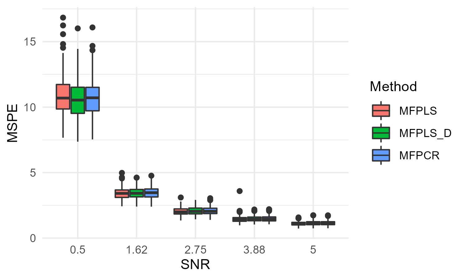
Figure 1: Boxplots of MSPE obtained by each approach in Setting 1.

All methods provide comparable results. In other words, our approach and the direct one give equivalent results. So in the following finite sample studies, we will use MFPLS.

3.1.2 Setting 2: binary response

In the following experiment, we focus on a classification problem with one-dimensional domain $\mathcal{I}=[0,50]$.
Here, we build two different classes (Class 1 and Class 2) of functional data, visualized in Figure 3. They are related to some pattern (a shape with peaks) appearing at some locations of the curves. This simulation setting is a kind of visual pattern-recognition problem (Fukushima, 1988). The pattern of interest is identifiable by eyes but challenging to detect with algorithms. An example may be epileptic spikes detection in electroencephalogram recordings (see for instance Abd El-Samie . (2018) for more details).
The performances of MFPLS, TMFPLS, and linear discriminant analysis on principal component scores (MFPCA-LDA) are compared in this simulation study.

Consider the domain $\mathcal{I}=[0,50]$, and the 2-dimensional functional predictor $X=(X^{(1)},X^{(2)})^{\operatorname*{\top}1}$ :

$$X^{(1)}(t)=\sum_{s=1}^{4}a_{s}h_{s}(t)+\epsilon^{(1)}(t)\;,X^{(2)}(t)=\sum_{s=1}^{4}(1-a_{s})h_{s}(t)+\epsilon^{(2)}(t)$$

where $\{a_{s}\}_{s=1}^{4}$ are discrete variables with values in $\{-1,0,1\}$, $\{h_{s}\}_{s=1}^{4}$ are the set of triangle function $h_{s}(t)=\left(1-0.25|t-10s|\right)_{+}$ $s=1,\ldots,4$ and $\epsilon=(\epsilon^{(1)},\epsilon^{(2)})^{\top}$ is a bivariate error function.

The error term is generated similarly as Happ  Greven (2018) framework. It consists in simulating a bivariate functional variable $e(.)=\sum_{k=1}^{100}\theta_{k}\phi_{k}(.)$ where $\{\phi_{k}\}_{k=1}^{100}$ are based on shifts of the first $100$ Fourier basis functions, $\theta_{k}$ are independent centered variables with variance $\sigma_{\theta,k}^{2}=\frac{101-k}{100}$ (for more details, see Happ  Greven (2018)). Then, the residual function is given by

$$\epsilon(.)=\sqrt{\frac{2}{101}}e(.).$$

This leads to have $\sum_{k=1}^{100}\langle\langle\epsilon,\phi_{k}\rangle\rangle\sim\mathcal{N}(0,1)$.

The discrete random variables $\{a_{j}\}_{j=1}^{4}$ are generated such as the probability of $a_{j+1}$ depends only on the value of $a_{j}$, $j=1,\ldots,3$. In addition, the probability of two consecutive variables is given by

$$\mathbb{P}(a_{j+1} =k|a_{j}=k,Z=z)=p_{j+1,z}$$

$$\text{ and }\mathbb{P}(a_{j+1} =k|a_{j}\neq k,Z=z)=\frac{1}{2}(1-p_{j+1,z})$$

where $j=1,2,3$, $k=-1,0,1$, and $Z\sim\mathcal{B}(p)$, with $p=\mathbb{P}(Z=1)$.
Let $p_{1,z}^{+},p_{1,z}^{+}\in[0,1]$ be

$$p_{1,z}^{+}=\mathbb{P}(a_{1}=1|Z=z),\text{ and }\text{ }p_{1,z}^{-}=\mathbb{P}(a_{1}=-1|Z=z).$$

Finally, $Y$ is defined as

$$Y=\left\{\begin{array}[]{ll}1&\mbox{if }a_{1}a_{2}-\left(|a_{3}|+|a_{4}|\right)=1\text{ or }a_{2}a_{3}-\left(|a_{1}|+|a_{4}|\right)=1\textbf{ }\\ 0&\mbox{ otherwise.}\end{array}\right.$$

If $a_{s}\neq 0$, $s=1,\ldots,4$, this means we observe a peak on $X^{(1)}$ at the position $t=10s$, which could be positive ($a_{s}=1$) or negative ($a_{s}=-1$). Then, $Y=1$, if strictly two consecutive peaks (both negatives or positives) occur at the beginning of $X^{(1)}$, namely the peaks of interest, are observed at $t=10,20$ or $t=20,30$. The four cases where $Y=1$ are illustrated in Figure 2.
Using the definition of the variables $\{a_{s}\}_{s=1}^{4}$, a direct calculation provides the probability $\mathbb{P}(Y=1)$ (see Appendix A for details).

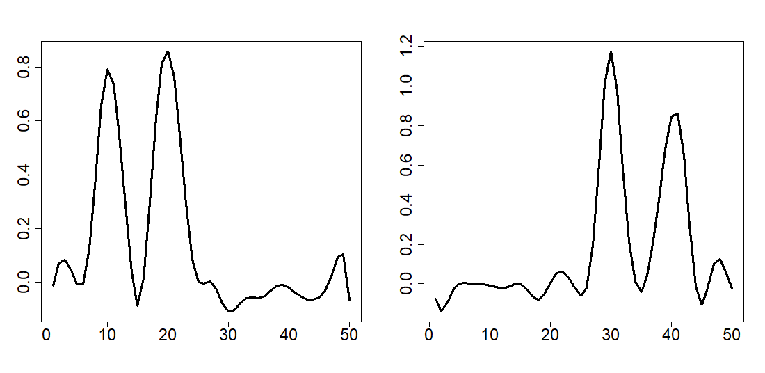
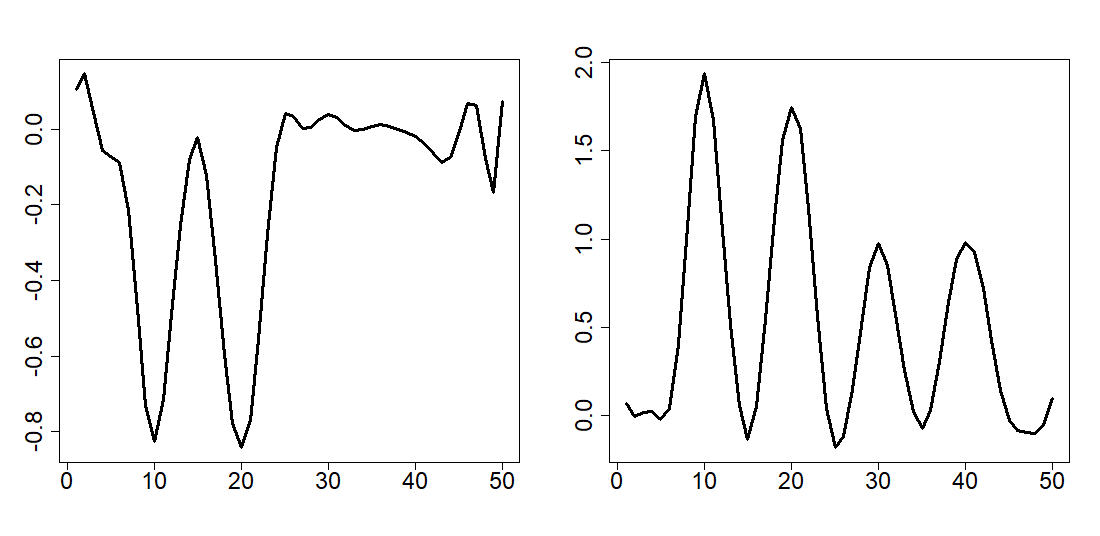
(1): $a_{1}$= $a_{2}$=1, and $a_{3}=a_{4}=0$	(2): $a_{1}$= $a_{2}$=-1, and $a_{3}=a_{4}=0$
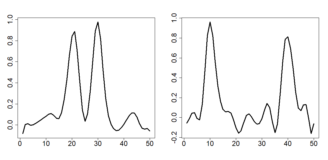
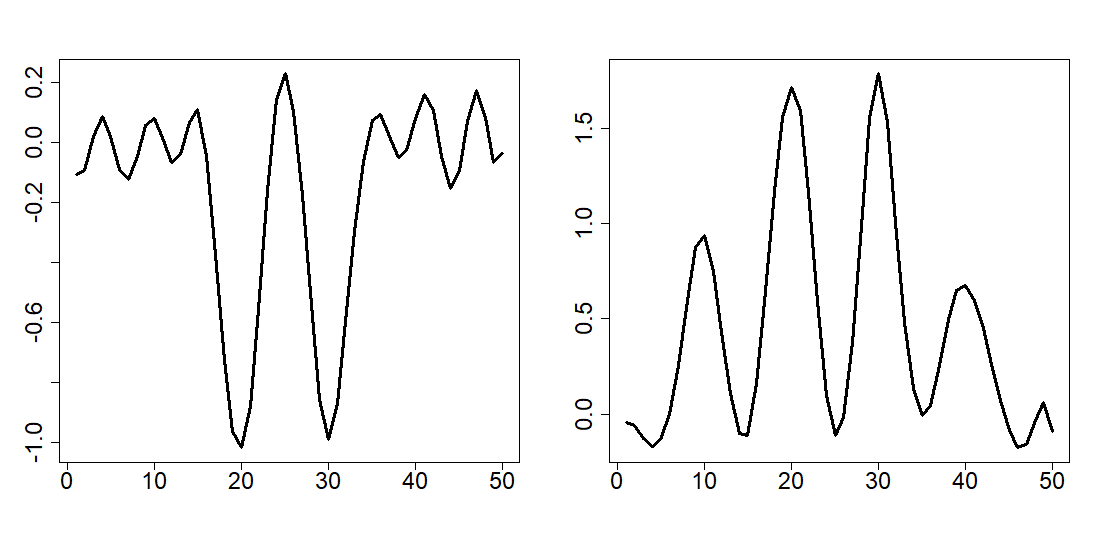
(3): $a_{2}$= $a_{3}$=1, and $a_{1}=a_{4}=0$	(4): $a_{2}$= $a_{3}$=-1, and $a_{1}=a_{4}=0$

Figure 2: Example of $Y=1$ (Setting 2)

.

Two scenarios are studied, and parameters used for numerical simulation are presented in Table 1. For each one, $N=500$ copies of $X$ are considered, and for each dimension, $50$ equidistant discrete times points on $\mathcal{I}$ of $X$ are observed.

Parameters	Scenario 1		Scenario 2
$p$	0.01		0.5
$Z$	0	1	0	1
$p_{1,z}^{+}$	0.890	0.450	0.450	0.005
$p_{1,z}^{-}$	0.010	0.450	0.450	0.005
$p_{2,z}$	0.900	0.010	0.900	0.010
$p_{3,z}$	0.010	0.900	0.010	0.900
$p_{4,z}$	0.900	0.010	0.900	0.010
$\hat{\mathbb{P}}(Y=1)$	0.344		0.424

Table 1: Parameters used to simulate scenarios 1 and 2.

	Scenario 1	Scenario 2
$Y=0$
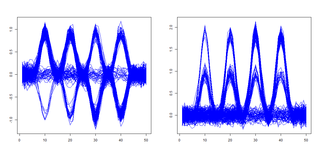
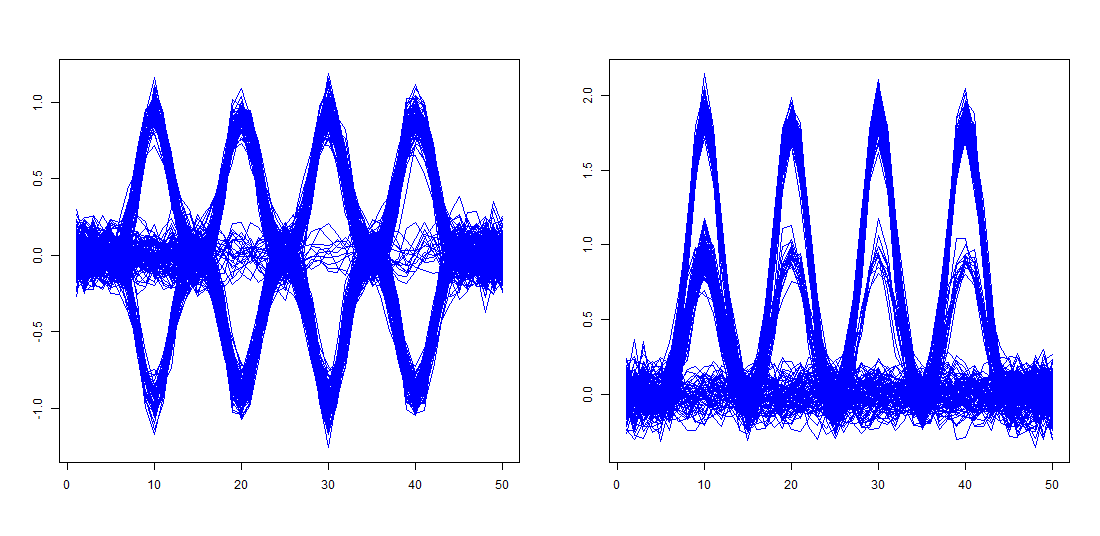
$Y=1$

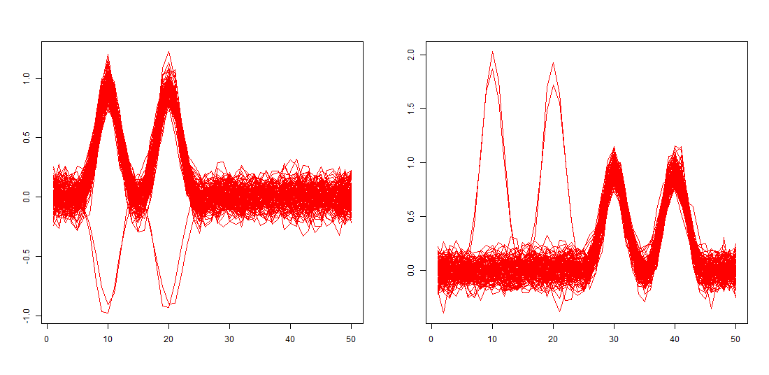
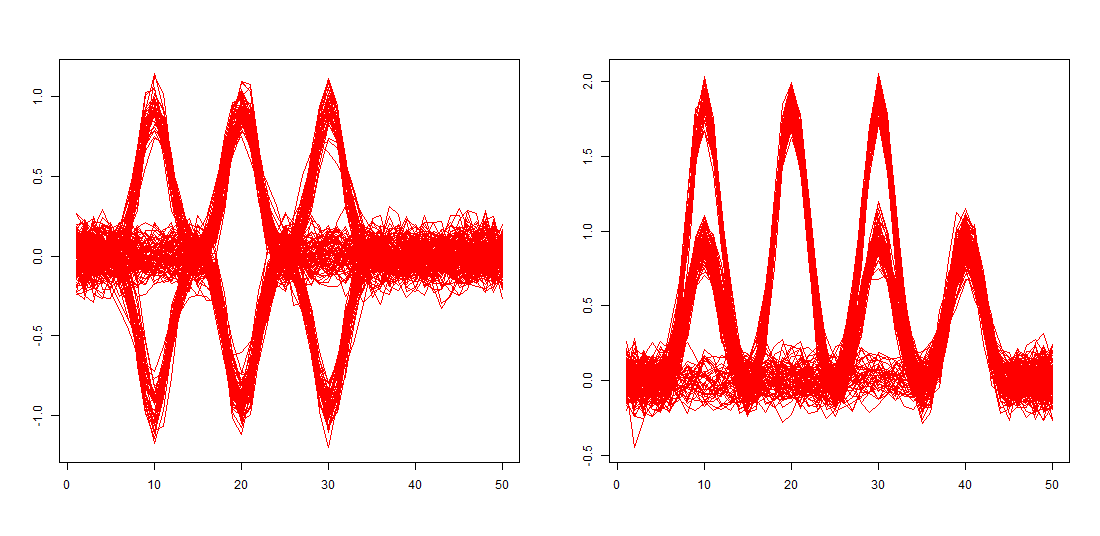
Figure 3: Example of curves $X$ in Setting 2, under both scenarios. Class 1 curves are in red and class 0 curves are in blue. The second scenario (right) shows more heterogeneity in class 1 compared to the first scenario (left).

Remark 4.

• In scenario 1, the $X$ curves are mainly related to the $Z=0$ regime, and class 1 ($Y=1$) is almost entirely composed of curves with shapes related to the (1) case of Figure 2, then we have two consecutive positive peaks at $t=10,20$ in $X^{(1)}$ (See Figure 3).

• Scenario 2 is more complex, both regimes of $Z$ have the same probability to occur.

  The regime $Z=0$ is related to case (1) (two consecutive positive peaks at $t=10,20$ in $X^{(1)}$) and case (2) (two consecutive negative peaks at $t=10,20$ in $X^{(1)}$ ).

  The regime $Z=1$ is related to case (3) (two consecutive positive peaks at $t=20,30$ in $X^{(1)}$) and case (4) (two consecutive negative peaks at $t=20,30$ in $X^{(1)}$).

The functional form of $X$ is reconstructed using 20 quadratic spline functions with equidistant knots (see Figure 3). For a given scenario, we did 200 experiments. At each, 75 % of the data are used for learning and 25 % for validation. The number of components for the MFPLS (in both models) is chosen by 10-fold cross-validation. Moreover, MFPCA-LDA is performed for comparison. It consists, firstly in the estimation of principal components (using Happ (2017) package) and then applying linear discriminant analysis to them. As in the previous model, the number of components is chosen by 10-fold cross-validation. By defining the set of groups as $\mathcal{G}_{1}=1,\mathcal{G}_{2}=2,\mathcal{G}_{3}=\{1,2\}$, the decision tree looks for the best splits among those obtained using separately univariate functions and the ones obtained using both dimensions. In order, to have an estimation of the optimal depth $m^{*}$, we randomly take 75% of learning data to train an intermediate TMFPLS, and 25% for pruning (by AUC metric). This procedure is repeated $10$ times and $\hat{m}^{*}$ is the frequent value among the $10$ repetitions. The final tree is then trained on the whole learning data, with the maximum tree depth fixed to $\hat{m}^{*}$, and the minimum criterion of impurity at 1%.

Results

		AUC	Sensibility	Specificity
Scen 1	MFPLS	83.39	96.4	65.62
	TMFPLS	93.90	97.14	88.78
	MFPCA-LDA	92.60	100	80.34
Scen 2	MFPLS	50.79	60.61	41.13
	TMFPLS	81.99	87.67	76.27
	MFPCA-LDA	50.00	60.17	40.00

Table 2: Metrics are the medians of the 200 replications on each validation set. The highest AUC by scenario is underlined.

In the first scenario, Table 2 shows AUC differences are about 10% between MFPLS and TMFPLS. Furthermore, MFPCA-LDA is competitive with TMFPLS. The second scenario shows more differences between the two methods, MFPLS and MFPCA-LDA are non-effective compared to TMFPLS. Hence, TMFPLS outperforms these methods in a complex task classification such as scenario 2.

In the supplementary materials, we analyze examples of trees (randomly selected among the 200 estimated) obtained from the two scenarios.

3.2 Different domains case

3.2.1 Setting 3: Image and Time series classification

Our approach allows the use of images and time series simultaneously. In this part, we highlight the use of various domains instead of focusing only on one dimension domain.

Framework

Consider the domains $\mathcal{I}_{1}=[0,50]$, $\mathcal{I}_{2}=[0,1]\times[0,1]$, and $X=(X^{(1)},X^{(2)})^{\operatorname*{\top}1}$:

$$X^{(1)}(t) =Z_{1}h(t)+\epsilon^{(1)}(t)\text{, }t\in\mathcal{I}_{1}$$

$$X^{(2)}(t) =Z_{2}q(t)+\epsilon^{(2)}(t)\text{, }t\in\mathcal{I}_{2}.$$

The noise term $\epsilon=(\epsilon^{(1)},\epsilon^{(2)})^{\top}$ is composed of two independent dimensions: the first one $\epsilon^{(1)}$ is a white noise of variances $\sigma^{2}$, while the second one $\epsilon^{(2)}$ is a gaussian random field. $\epsilon^{(2)}$ is associated with a Matern covariance model, with sill, range, and nugget parameters equal to $0.25$, $0.75$, and $\sigma$, respectively (see Ribeiro Jr . (2001) for more details). The variables $Z_{1}$ and $Z_{2}$ are Bernoulli variables with values in $\{0,1\}$. The (deterministic) functions $h$ and $q$ are given by:

$$\;h(t) =3.14\left(1-\frac{|t-10|}{4}\right)_{+} q(s) =-2\log\left(\sqrt{(s^{(1)}-0.5)^{2}+(s^{(2)}-0.5)^{2}}\right)$$

where $(.)_{+}$ denotes the positive part, $t\in\mathcal{I}_{1}$, $s=(s^{(1)},s^{(2)})\in\mathcal{I}_{2}$.
The response variable $Y$ is constructed as follows :

$$Y=\left\{\begin{array}[]{ll}1&\mbox{if }Z_{1}Z_{2}=1\\ 0&\mbox{ otherwise.}\end{array}\right.$$

In other words, $Y=1$ if and only if both variables $Z_{1}$, $Z_{2}$ are simultaneously 1 (see Figure 4).

$X^{(1)}(t)$		+		=
$X^{(2)}(t)$		+		=

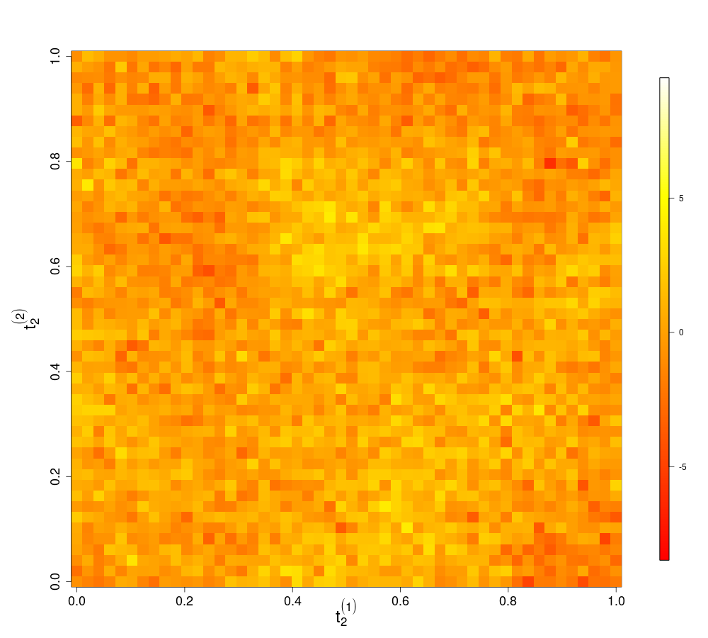
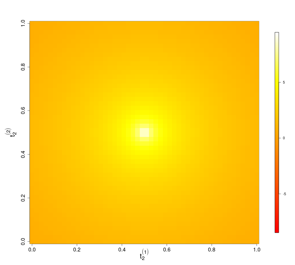
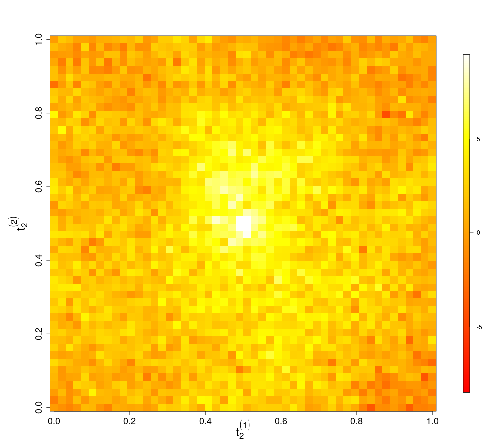
Figure 4: Construction of class 1 ($Y=1$), curve $X(t)$ in Setting 3, under SNR=$0.5$

If $Y$=0, $X$ is random noise $\epsilon$ (left figures).

$50$ equidistant discrete points and $50\times 50$ pixels are observed respectively for the first and the second dimension. To get the functional form of $X$, the first and second components are projected respectively into the space spanned by $20$ quadratic spline functions, and the 4 two-dimensional splines (Happ, 2017).
The variances of the functions $q$ and $h$ along their domain are approximately 1. The signal-to-noise ratio (SNR) is then (approximately) the same on both dimensions and depends only on $\sigma$

$$\text{SNR}=\frac{1}{\sigma^{2}}.$$

By controlling the parameter $\sigma$, we consider several values of SNR: $0.5$, $0.7$, $1.2$, $2.1$ and $4.9$ .

We set $\mathbb{P}(Z_{1}=1)=\mathbb{P}(Z_{2}=1)=3/4$, then $\mathbb{P}(Y=1)=9/16\simeq 0.56$. A set of 500 curves are simulated: 75% are used for learning, while the remaining 25% is for the validation set.

For each value of SNR, three MFPLS models are computed. The two first use exclusively one dimension of the predictor: MFPLS(1) uses $X^{(1)}$ and MFPLS(2) $X^{(2)}$. The third one uses both functional components (MFPLS). The purpose is to assess the amount of performance using one-dimensional domain and multiple-dimensional domain. We also compute MFPCA-LDA for comparison purposes, the principal component analysis is performed by Happ (2017) package.
The number of components in the two approaches: MFPLS and MFPCA-LDA are chosen by 10-fold cross-validation using AUC. We did 200 simulations: models are assessed by AUC on the validation set.

Figure 5: Boxplots of obtained AUC on the validation set.

Figure 5 shows that MFPLS gives better results than MFPCA-LDA for the lowest value of SNR, and the difference between the methods disappears with the increase of SNR. Using partially the data (models MFPLS(1) and MFPLS(2)) to predict the class variable is less efficient than using both dimensions. Namely, Figure 5 clearly shows the advantage of using both of the components of the functional variables.

This simulation demonstrates the ability of our method to classify different domain data. In addition, as it’s specially designed for supervised learning, it can be more effective than principal component analysis-based techniques such as MFPCA-LDA in a noisy context.

4 Real data application: Multivariate time series classification

In this section, we compare the proposed methods with black box models (LSTM, Random Forest, etc…) on benchmark data (Table 3, from Table 1 of (Karim ., 2019)), ranging from online character recognition to activity recognition. These data, suitable for multivariate functional time series data and binary classification, have been used by various works to assess new methodologies (see e.g Pei . (2017), Schäfer  Leser (2017)).

Dataset	d	T	Task	Ratio	Sources
CMUsubject16	62	534	Action Recognition	50-50 split	Carnegie (0)
ECG	2	147	ECG Classification	50-50 split	Oleszewski (2012)
EEG	13	117	EEG Classification	50-50 split	Lichman (2013)
EEG2	64	256	EEG Classification	20-80 split	(Lichman, 2013)
KickvsPunch	62	761	Action Recognition	62-38 split	Carnegie (0)
Movement AAL	4	119	Movement Classification	50-50 split	Lichman (2013)
NetFlow	4	994	Action Recognition	60-40 split	Sübakan . (2014)
Occupancy	5	3758	Occupancy Classification	35-65 split	Lichman (2013)
Ozone	72	291	Weather Classification	50-50 split	Lichman (2013)
Wafer	6	198	Manufacturing Classification	25-75 split	Oleszewski (2012)
WalkVsRun	62	1918	Action Recognition	64-36 split	Carnegie (0)

Table 3: Datasets summary. T denotes the number of sampling time points, d: the data dimensions, and Ratio of the train-test split. All datasets are available in https://github.com/titu1994/MLSTM-FCN/releases/tag/v1.0

The proposed models (MFPLS, TMFPLS) are compared with discriminant analysis (MFPCA-LDA) on scores obtained by Multivariate functional principal component analysis (Happ, 2017), and non-functional models; the Long Short-Term Memory Fully Convolutional Network (LSTM-FCN) and Attention LSTM-FCN (ALSTM-FCN), proposed by Karim . (2019). We also present the benchmark of these last models named SOTA, which gives the best performances among Dynamic time warping (DTW), Random Forest (RF), SVM with a linear kernel, SVM with a 3rd-degree polynomial kernel (SVM-Poly), and other state-of-the-art methods (see Karim . (2019) for more details).
The challenge is to show that our models based on regression can be competitive. The splitting of the data into training and test samples (see Table 3) is that of Karim . (2019). The different models mentioned above are compared by the accuracy metric, the rate of well-predicted classes obtained on the test datasets.

4.1 Choice of hyperparameters

As for some datasets (CMUsubject, KickVsPunch, etc…), the sample size is small (less than $50$ observations, see Table 4) the number of components in MFPLS and MFPCA is chosen by 20-fold cross-validation (contrary to $10$-fold in previous parts). The maximum tree depth $m^{*}$ is an important hyperparameter. It may significantly affect the performance of our tree-based model, as it helps to prevent the overfitting of TMFPLS. We estimate $m^{*}$ by cross-validation alike procedure. More precisely, we randomly take 75% of learning data to train an intermediate TMFPLS and 25% for pruning. This procedure is repeated $10$ times and let $\hat{m}^{*}$ be the most occurred number from these $10$. The final tree is then trained on the whole learning data, with the maximum tree depth fixed to $\hat{m}^{*}$. As in the previous section, group are defined as $\mathcal{G}_{1}=1,\ldots,\mathcal{G}_{d}=d,\mathcal{G}_{d+1}=\{1,...,d\}$, to see whether FPLS gives better splitting than MFPLS. Testing several combinations of dimensions takes time, the ideal choice of groups would be guided by some prior knowledge of the data structure.
Two strategies are used for the number of components in the decision tree: TMFPLS H-1 denotes the decision tree where only one component in MFPLS is used, and TMFPLS H-CV is the decision tree where the number of components is estimated by 20-fold cross-validation as in MFPLS. The first tree is faster to train than the second one, and it’s less likely to overfit the data. However, the second one is expected to be a more efficient model, since it is able to estimate more complex coefficient functions $\beta$.

For all functional data methods, we use 30 B-Splines basis functions by dimension to have a functional representation (Ramsey  Silverman, 2005) of each dataset (see Figure 5 in the supplementary materials for the smoothed functions). This number of basis functions is chosen arbitrarily small compared to the minimum number of discrete time points ($117$) of the original raw datasets.

4.2 Results

Table 4 shows that, in most cases, our models (MFPLS, TMFPLS) and MFPCA-LDA are competitive with that of Karim . (2019) and SOTA. In about half of the cases, TMFPLS or MFPLS reach the highest or the second-highest accuracy. TMFPLS is generally more performant than MFPLS. Note also that MFPCA-LDA is competitive with the proposed methodologies. The main difference between MFPCA-LDA and MFPLS is that for the first one components are searched with no regard to the response variable $Y$.
For the KickVsPunch dataset, the performance of TMFPLS H-1 is better than the one by TMFPLS H-CV. This is because TMFPLS H-CV could easily overfit when the training sample is small ($\text{N}_{\text{Train}}<20$). This is one of the well-known drawbacks of the decision tree. Tuning hyperparameters is then crucial and may have a huge impact on performances.

Datasets	$\textbf{N}_{\textbf{Train}}$	$\textbf{N}_{\textbf{Test}}$	MFPLS	TMFPLS H-1	TMFPLS H-CV	MFPCA-LDA	Karim .	SOTA	Methods
CMUsubject16	29	29	86.21	89.66	100	89.66	100	100	[1]
ECG	100	100	85	83	87	88	86	93	[2]
EEG	64	64	48.44	54.69	53.12	46.88	65.63	62.5	[3]
EEG2	600	600	81.83	68.67	82.67	72.17	91.33	77.5	[3]
KickVsPunch	16	10	90	90	60	80	100	100	[2]
MovementAAL	157	157	67.52	56.69	53.50	61.78	79.63	65.61	[4]
NetFlow	803	534	84.64	86.52	85.77	80.90	95	98	[2]
Occupancy	41	76	71.05	61.84	59.21	80.26	76	67.11	[4]
Ozone	173	173	73.99	73.41	73.41	79.19	81.5	75.14	[5]
Wafer	298	896	85.04	87.39	97.99	97.32	99	99	[2]
WalkVsRun	28	16	100	100	100	100	100	100	[2]

Table 4: Comparison of MFPLS, TMFPLS, and other non-FDA classification methods by their accuracies (%) in the test set.
[1]: Tuncel  Baydogan (2018), [2]:Schäfer  Leser (2017), [3]:RF , [4]: SVM-Poly, [5]: DTW

5 Conclusion and discussion

Statistical learning of multivariate functional data evolving in complex spaces leads to challenging questions that need the development of new methods and techniques. In this paper, we are interested in some of these methods in the case of different functional domain settings. Namely, we propose least squares regression and classification models for multivariate functional predictors. The first classification model relies on the partial least square (PLS) regression (MFPLS) while the second one (TMFPLS) combines PLS with a decision tree. Technical arguments on the PLS methods are given. The finite sample performance of the regression and classification models are assessed by simulations and real data (EEG, Ozone, wafer,…) applications where we compare the proposed methods with some benchmarks, in particular a PLS regression model of the literature (Beyaztas  Shang (2022)) and well known principal components regression and some machine learning models.
A main specificity of our proposed models is that the multivariate functional data considered are defined on different domains compared to the literature. This allows dealing with heterogeneous types of data (e.g. images, time series, etc.) with a potentially large number of applications as shown by the given classification case study on images and functional time series. We also give a relationship between the partial least square of multivariate functional data with its univariate counterparts. To the best of our knowledge, the proposed tree classification model is new.

The finite sample properties show our models’ competitiveness with regard to some existing methods. The multivariate time series classification case study highlights the competitive performance of MFPLS and TMFPLS with black-box models (LSTM, RF,…) on benchmark data. These performances may be improved by using prior knowledge of the benchmark data (groups of variables, suitable preprocessing, …).
In this paper we focus on continuous functional predictors, a possible extension of the proposed models would be including additional type (e.g, qualitative) of covariates.
The EEG and ozone data considered in the finite sample study may have spatial dependence. The classification approaches seem not affected by these data dependencies, but this deserves future investigation.
As in a number of functional data analysis, a tuning parameter related to the number of basis functions used to smooth the raw data or reduce the dimension of the functional space, has to be selected. In this paper, we fix or use a cross-validation approach for the choice of this parameter. Other alternatives may be based on bootstrap methods or criteria like AIC, BIC.

This work highlights the good behavior of TMFPLS and a way to deal with non-linearity in classification problems of multivariate functional data. However, with heterogeneous high-dimensional data, tree-based methods may be challenging. An alternative method could be cluster-wise regression techniques by extending the univariate case studied by Preda  Saporta (2005) to our context. Some other methods as lasso classification techniques can also be explored (see e.g Godwin (2013)).

Supplementary information The supplementary material includes additional figures related to the numerical experiments.

Appendix A Technical arguments

Proof of Proposition 8.

Here C-S (1) and C-S (2) stand respectively for Cauchy-Schwartz inequality on integrals and sums.

$$\text{Cov}^{2}(\langle\langle X,w\rangle\rangle,Y) =\mathbb{E}^{2}\left(\langle\langle X,w\rangle\rangle Y\right)$$

$$=\left[\sum_{j=1}^{d}\left[\int_{\mathcal{I}_{j}}\mathbb{E}\left(X^{(j)}(t)Y\right)w^{(j)}(t)dt\right]\right]^{2}$$

$$\text{ \scriptsize C-S(1)}\implies\text{Cov}^{2}(\langle\langle X,w\rangle\rangle,Y) {\leq}\left[\sum_{j=1}^{d}\left(\int_{\mathcal{I}_{j}}\mathbb{E}^{2}(X^{(j)}(t)Y)dt\right)^{1/2}\right.$$

$$\indent\indent\left.\left(\int_{\mathcal{I}_{j}}[w^{(j)}(t)]^{2}dt\right)^{1/2}\right]^{2}$$

$$\text{ \scriptsize C-S (2) }\implies\text{Cov}^{2}(\langle\langle X,w\rangle\rangle,Y) \leq\left[\sum_{j=1}^{d}\int_{\mathcal{I}_{j}}\mathbb{E}^{2}(X^{(j)}(t)Y)dt\right]\underbrace{\left[\sum_{j=1}^{d}\int_{\mathcal{I}_{j}}[w^{(j)}(t)]^{2}dt\right]}_{|||w|||^{2}=1}$$

$$\text{Cov}^{2}(\langle\langle X,w\rangle\rangle,Y) \leq\sum_{j=1}^{d}\int_{\mathcal{I}_{j}}\mathbb{E}^{2}(X^{(j)}(t)Y)dt$$

The C-S inequalities become equalities, meaning the maximums are reached, if for $j=1,\ldots,d$ there exist non-null scalars $a$ and $a^{\prime}$ such as:

• $\displaystyle w^{(j)}(t)=a\mathbb{E}(X^{(j)}(t)Y),t\in\mathcal{I}_{j}$

• $\displaystyle\left(\int_{\mathcal{I}_{j}}[w^{(j)}(t)]^{2}dt\right)^{1/2}$ $=a^{\prime}\left(\int_{\mathcal{I}_{j}}\mathbb{E}^{2}(X^{(j)}(t)Y)dt\right)^{1/2}$.

The first condition implies the second one, indeed if $\displaystyle w^{(j)}(t)=a\mathbb{E}(X^{(j)}(t)Y)$ then $\displaystyle\left(\int_{\mathcal{I}_{j}}[w^{(j)}(t)]^{2}dt\right)^{1/2}=|a|\left(\int_{\mathcal{I}_{j}}\mathbb{E}^{2}(X^{(j)}(t)Y)dt\right)^{1/2}$, hence $a^{\prime}=|a|$.
To have $|||w|||=1$, we take $a=\displaystyle\left(\sum_{j=1}^{p}\int_{\mathcal{I}_{j}}\mathbb{E}^{2}(X^{(j)}(t)Y)dt\right)^{-1/2}$.
Thus, the solution of (7) is

$$w^{(j)}(t)=\frac{\mathbb{E}(X^{(i)}(t)Y)}{\left(\sum_{j=1}^{p}\int_{\mathcal{I}_{j}}\mathbb{E}^{2}(X^{(j)}(t)Y)dt\right)^{1/2}},\;t\in\mathcal{I}_{j}.$$ (18)

∎

Proof of Proposition 2.

$X$ first order residual definition is $X=\xi_{1}\rho_{1}+X_{1}$, where $X_{1}$ holds

$$\mathbb{E}(\xi_{1}X_{1})=0_{\mathbb{R}^{d}}\iff\mathbb{E}(\xi_{1}X_{1}^{(j)}(t))=0\;t\in\mathcal{I}_{j},\;1\leq j\leq d.$$ (19)

Analogously higher-order residuals also verify

$$\mathbb{E}(\xi_{h}X_{h})=0_{\mathbb{R}^{d}}\text{ }\forall h\in\mathbb{N}^{*}.\\$$ (20)

To show that $\{\xi_{k}\}_{k=1}^{h}$ forms an orthogonal system, we use a proof by induction, similarly to Tenenhaus . (1995).

The base case verifies. Indeed, (19) implies that

$$\mathbb{E}(\xi_{1}\xi_{2})=\sum_{j=1}^{d}\int_{\mathcal{I}_{j}}\mathbb{E}\left(\xi_{1}X_{1}^{(j)}(t)\right)w_{2}^{(j)}(t)dt=0.$$

Assume the induction hypothesis $\mathcal{H}_{0}$, $\mathcal{H}_{0}$: $\{\xi_{k}\}_{k=1}^{h}$ forms an orthogonal system $h\geq 1$

$$\mathbb{E}(\xi_{h}\xi_{h+1}) =\sum_{j=1}^{d}\int_{\mathcal{I}_{j}}\mathbb{E}\left(\xi_{h}X_{h}^{(j)}(t)\right)w_{h+1}^{(j)}(t)dt$$

$$(\ref{h_orthog})\implies\mathbb{E}(\xi_{h}\xi_{h+1}) =0$$

$$\mathbb{E}(\xi_{h-1}\xi_{h+1}) =\sum_{j=1}^{d}\int_{\mathcal{I}_{j}}\mathbb{E}\left(\xi_{h-1}X_{h}^{(j)}(t)\right)w_{h+1}^{(j)}(t)dt$$

$$\text{Since }X_{h-1}=\rho_{h}\xi_{h}+X_{h}$$

$$\implies\mathbb{E}(\xi_{h-1}\xi_{h+1}) =\sum_{j=1}^{d}\int_{\mathcal{I}_{j}}\underbrace{\mathbb{E}\left(\xi_{h-1}X_{h-1}^{(j)}(t)\right)}_{=0\text{ by }(\ref{h_orthog})}dt$$

$$\;\;-\rho_{h}^{(j)}(t)\int_{\mathcal{I}_{j}}\underbrace{\mathbb{E}\left(\xi_{h-1}\xi_{h}\right)}_{=0\text{ by }\mathcal{H}_{0}}\sum_{j=1}^{d}w_{h+1}^{(j)}(t)dt,$$

$$\text{then }\mathbb{E}(\xi_{h-1}\xi_{h+1}) =0$$

The same procedure can be used to show that $\mathbb{E}(\xi_{j}\xi_{h+1})$ = 0 $\forall j\leq h-2$. Hence, $\{\xi_{k}\}_{k=1}^{h}$ forms an orthogonal system $\forall h\geq 1$.
The expansion formulas are implications of this point. ∎

Proof of Lemma 1 .

For $h=1$, we have $v_{1}=w_{1}$, as $\xi_{1}=\langle\langle X,w_{1}\rangle\rangle$, the base case verifies.
Assume that $\langle\langle X,v_{j}\rangle\rangle=\xi_{j}$ is true up to order $h$ ($\forall j\leq h$).
Recall that,

$$\xi_{h+1}=\langle\langle X_{h},w_{h+1}\rangle\rangle.$$ (21)

The second equation of Proposition 2, gives that

$$X_{h}=X-\sum_{i=1}^{h}\rho_{i}\langle\langle v_{i},X\rangle\rangle$$

.
Then

$$\begin{split}\xi_{h+1}=\langle\langle X,w_{h+1}\rangle\rangle-\sum_{i=1}^{h}\langle\langle v_{i},X\rangle\rangle\langle\langle\rho_{i},w_{h+1}\rangle\rangle=\langle\langle X,\underbrace{w_{h+1}-\sum_{i=1}^{h}\langle\langle\rho_{i},w_{h+1}\rangle\rangle v_{i}}_{v_{h+1}}\rangle\rangle\end{split}$$

This concludes the proof.
∎

Calculus of $\mathbb{P}(Y)$ in details.

From the definition of $Y$ $\mathbb{P}(Y=1)=\mathbb{P}(S_{1})+\mathbb{P}(S_{2})$, since $\mathbb{P}(S_{1}\cap S_{2})=0$ where

$$S_{1}^{+} =\{a_{1}=1,a_{2}=1,a_{3}=0,a_{4}=0\} S_{1}^{-} =\{a_{1}=-1,a_{2}=-1,a_{3}=0,a_{4}=0\}$$

$$S_{2}^{+} =\{a_{1}=0,a_{2}=1,a_{3}=1,a_{4}=0\} S_{2}^{-} =\{a_{1}=0,a_{2}=-1,a_{3}=-1,a_{4}=0\},$$

$S_{1}=S_{1}^{+}\cup S_{1}^{-}$, and $S_{2}=S_{2}^{+}\cup S_{2}^{-}$.

$$\mathbb{P}(S_{1}^{+}) =\mathbb{P}(a_{4}=0|a_{3}=0,a_{2}=1,a_{1}=1)$$

$$\indent\mathbb{P}(a_{3}=0|a_{2}=1,a_{1}=1)\mathbb{P}(a_{2}=1|a_{1}=1)\mathbb{P}(a_{1}=1)$$

$$\mathbb{P}(S_{1}^{+}) =\mathbb{P}(a_{4}=0|a_{3}=0)$$

$$\indent\mathbb{P}(a_{3}=0|a_{2}=1)\mathbb{P}(a_{2}=1|a_{1}=1)\mathbb{P}(a_{1}=1).$$

The same procedure gives $\mathbb{P}(S_{1}^{-})$, $\mathbb{P}(S_{2}^{+})$, and $\mathbb{P}(S_{2}^{-})$. Using conditional probability to Z, we obtain

$$\mathbb{P}(S_{1}|Z=z) =\mathbb{P}(S_{1}^{+}|Z=z)+\mathbb{P}(S_{1}^{-}|Z=z)=\frac{1}{2}p_{4,z}p_{2,z}(1-p_{3,z})p_{1,z}$$

$$\mathbb{P}(S_{2}|Z=z) =\mathbb{P}(S_{2}^{+}|Z=z)+\mathbb{P}(S_{2}^{-}|Z=z)=\frac{1}{2}(1-p_{4,z})p_{3,z}(1-p_{2,z})(1-\rho_{1,z}).$$

Finally, the law of total probability yields to

$$\begin{split}\mathbb{P}(Y=1)=(1-p)\left[\frac{1}{2}p_{4,0}p_{2,0}(1-p_{3,0})p_{1,0}+\frac{1}{2}(1-p_{4,0})p_{3,0}(1-p_{2,0})(1-p_{1,0})\right]\\ +p\left[\frac{1}{2}p_{4,1}p_{2,1}(1-p_{3,1})p_{1,1}+\frac{1}{2}(1-p_{4,1})p_{3,1}(1-p_{2,1})(1-p_{1,1})\right]\end{split}$$

∎

References

- \bibcommenthead
- Abd El-Samie \BOthers. (\APACyear2018) \APACinsertmetastarspikes{APACrefauthors}Abd El-Samie, F.E., Alotaiby, T.N., Khalid, M.I., Alshebeili, S.A.\BCBL Aldosari, S.A. \APACrefYearMonthDay2018. \BBOQ\APACrefatitleA review of EEG and MEG epileptic spike detection algorithms A review of eeg and meg epileptic spike detection algorithms.\BBCQ \APACjournalVolNumPagesIEEE Access660673–60688. \PrintBackRefs\CurrentBib
- Aguilera \BOthers. (\APACyear2010) \APACinsertmetastarpls_exp{APACrefauthors}Aguilera, A.M., Escabias, M., Preda, C.\BCBL Saporta, G. \APACrefYearMonthDay2010. \BBOQ\APACrefatitleUsing basis expansions for estimating functional PLS regression: applications with chemometric data Using basis expansions for estimating functional pls regression: applications with chemometric data.\BBCQ \APACjournalVolNumPagesChemometrics and Intelligent Laboratory Systems1042289–305. \PrintBackRefs\CurrentBib
- Beyaztas \BBA Shang (\APACyear2022) \APACinsertmetastarMFPLS2022{APACrefauthors}Beyaztas, U.\BCBT \BBA Shang, H.L. \APACrefYearMonthDay2022. \BBOQ\APACrefatitleA Robust Functional Partial Least Squares for Scalar-on-Multiple-Function Regression A robust functional partial least squares for scalar-on-multiple-function regression.\BBCQ \APACjournalVolNumPagesJournal of Chemometricse3394. \PrintBackRefs\CurrentBib
- Blanquero \BOthers. (\APACyear2019\APACexlab\BCnt1) \APACinsertmetastarblanquero2019_2{APACrefauthors}Blanquero, R., Carrizosa, E., Jiménez-Cordero, A.\BCBL Martín-Barragán, B. \APACrefYearMonthDay2019\BCnt1. \BBOQ\APACrefatitleFunctional-bandwidth kernel for support vector machine with functional data: an alternating optimization algorithm Functional-bandwidth kernel for support vector machine with functional data: an alternating optimization algorithm.\BBCQ \APACjournalVolNumPagesEuropean Journal of Operational Research2751195–207. \PrintBackRefs\CurrentBib
- Blanquero \BOthers. (\APACyear2019\APACexlab\BCnt2) \APACinsertmetastarblanquero2019{APACrefauthors}Blanquero, R., Carrizosa, E., Jiménez-Cordero, A.\BCBL Martín-Barragán, B. \APACrefYearMonthDay2019\BCnt2. \BBOQ\APACrefatitleVariable selection in classification for multivariate functional data Variable selection in classification for multivariate functional data.\BBCQ \APACjournalVolNumPagesInformation Sciences481445–462. \PrintBackRefs\CurrentBib
- Cardot \BOthers. (\APACyear1999) \APACinsertmetastarcardot1999{APACrefauthors}Cardot, H., Ferraty, F.\BCBL Sarda, P. \APACrefYearMonthDay1999. \BBOQ\APACrefatitleFunctional linear model Functional linear model.\BBCQ \APACjournalVolNumPagesStatistics & Probability Letters45111–22. \PrintBackRefs\CurrentBib
- Carnegie (\APACyear0) \APACinsertmetastarcarn{APACrefauthors}Carnegie \APACrefYearMonthDay0. \APACrefbtitleCarnegie Mellon University- cmu graphics lab - motion capture library. Carnegie Mellon University- cmu graphics lab - motion capture library. \APAChowpublishedhttp://mocap.cs.cmu.edu/. \APACrefnoteAccessed: 2022-05 \PrintBackRefs\CurrentBib
- Delaigle \BBA Hall (\APACyear2012) \APACinsertmetastardelaigle2012{APACrefauthors}Delaigle, A.\BCBT \BBA Hall, P. \APACrefYearMonthDay2012. \BBOQ\APACrefatitleMethodology and theory for partial least squares applied to functional data Methodology and theory for partial least squares applied to functional data.\BBCQ \APACjournalVolNumPagesThe Annals of Statistics401322–352. \PrintBackRefs\CurrentBib
- Dembowska \BOthers. (\APACyear2021) \APACinsertmetastarFPLS0{APACrefauthors}Dembowska, S., Liu, H., Houwing-Duistermaat, J.\BCBL Frangi, A. \APACrefYearMonthDay2021. \BBOQ\APACrefatitleMultivariate functional partial least squares for classification using longitudinal data Multivariate functional partial least squares for classification using longitudinal data.\BBCQ \APACjournalVolNumPagesMultivariate functional partial least squares for classification using longitudinal data75–88. \PrintBackRefs\CurrentBib
- Escabias \BOthers. (\APACyear2004) \APACinsertmetastarescabias2004principal{APACrefauthors}Escabias, M., Aguilera, A.\BCBL Valderrama, M. \APACrefYearMonthDay2004. \BBOQ\APACrefatitlePrincipal component estimation of functional logistic regression: discussion of two different approaches Principal component estimation of functional logistic regression: discussion of two different approaches.\BBCQ \APACjournalVolNumPagesJournal of Nonparametric Statistics163-4365–384. \PrintBackRefs\CurrentBib
- Ferraty \BBA Vieu (\APACyear2003) \APACinsertmetastarferraty{APACrefauthors}Ferraty, F.\BCBT \BBA Vieu, P. \APACrefYearMonthDay2003. \BBOQ\APACrefatitleCurves discrimination: a nonparametric functional approach Curves discrimination: a nonparametric functional approach.\BBCQ \APACjournalVolNumPagesComputational Statistics & Data Analysis441161-173. \APACrefnoteSpecial Issue in Honour of Stan Azen: a Birthday Celebration \PrintBackRefs\CurrentBib
- Fukushima (\APACyear1988) \APACinsertmetastarvisual{APACrefauthors}Fukushima, K. \APACrefYearMonthDay1988. \BBOQ\APACrefatitleA neural network for visual pattern recognition A neural network for visual pattern recognition.\BBCQ \APACjournalVolNumPagesComputer21365–75. \PrintBackRefs\CurrentBib
- Galeano \BOthers. (\APACyear2015) \APACinsertmetastargaleano2015{APACrefauthors}Galeano, P., Joseph, E.\BCBL Lillo, R.E. \APACrefYearMonthDay2015. \BBOQ\APACrefatitleThe Mahalanobis distance for functional data with applications to classification The mahalanobis distance for functional data with applications to classification.\BBCQ \APACjournalVolNumPagesTechnometrics572281–291. \PrintBackRefs\CurrentBib
- Gardner-Lubbe (\APACyear2021) \APACinsertmetastarLDA{APACrefauthors}Gardner-Lubbe, S. \APACrefYearMonthDay2021. \BBOQ\APACrefatitleLinear discriminant analysis for multiple functional data analysis Linear discriminant analysis for multiple functional data analysis.\BBCQ \APACjournalVolNumPagesJournal of Applied Statistics48111917-1933. \PrintBackRefs\CurrentBib
- Godwin (\APACyear2013) \APACinsertmetastargodwin2013{APACrefauthors}Godwin, J. \APACrefYear2013. \APACrefbtitleGroup Lasso for Functional Logistic Regression Group lasso for functional logistic regression \APACtypeAddressSchool\BUMTh. \PrintBackRefs\CurrentBib
- Golovkine \BOthers. (\APACyear2022) \APACinsertmetastargolovkine{APACrefauthors}Golovkine, S., Klutchnikoff, N.\BCBL Patilea, V. \APACrefYearMonthDay2022. \BBOQ\APACrefatitleClustering multivariate functional data using unsupervised binary trees Clustering multivariate functional data using unsupervised binary trees.\BBCQ \APACjournalVolNumPagesComputational Statistics & Data Analysis168107376. \PrintBackRefs\CurrentBib
- Górecki \BOthers. (\APACyear2015) \APACinsertmetastargorecki{APACrefauthors}Górecki, T., Krzyśko, M.\BCBL Wołyński, W. \APACrefYearMonthDay2015. \BBOQ\APACrefatitleClassification problems based on regression models for multi-dimensional functional data Classification problems based on regression models for multi-dimensional functional data.\BBCQ \APACjournalVolNumPagesStatistics in Transition new series161. \PrintBackRefs\CurrentBib
- Guan \BOthers. (\APACyear2022) \APACinsertmetastarsparsefpls{APACrefauthors}Guan, T., Lin, Z., Groves, K.\BCBL Cao, J. \APACrefYearMonthDay2022. \BBOQ\APACrefatitleSparse functional partial least squares regression with a locally sparse slope function Sparse functional partial least squares regression with a locally sparse slope function.\BBCQ \APACjournalVolNumPagesStatistics and Computing3221–11. \PrintBackRefs\CurrentBib
- Happ (\APACyear2017) \APACinsertmetastarrMFPCA{APACrefauthors}Happ, C. \APACrefYearMonthDay2017. \BBOQ\APACrefatitleObject-oriented software for functional data Object-oriented software for functional data.\BBCQ \APACjournalVolNumPagesarXiv preprint arXiv:1707.02129. \PrintBackRefs\CurrentBib
- Happ \BBA Greven (\APACyear2018) \APACinsertmetastarhapp2018multivariate{APACrefauthors}Happ, C.\BCBT \BBA Greven, S. \APACrefYearMonthDay2018. \BBOQ\APACrefatitleMultivariate functional principal component analysis for data observed on different (dimensional) domains Multivariate functional principal component analysis for data observed on different (dimensional) domains.\BBCQ \APACjournalVolNumPagesJournal of the American Statistical Association113522649–659. \PrintBackRefs\CurrentBib
- Hochreiter \BBA Schmidhuber (\APACyear1997) \APACinsertmetastarLSTM{APACrefauthors}Hochreiter, S.\BCBT \BBA Schmidhuber, J. \APACrefYearMonthDay1997. \BBOQ\APACrefatitleLong Short-Term Memory Long short-term memory.\BBCQ \APACjournalVolNumPagesNeural Computation981735-1780. \PrintBackRefs\CurrentBib
- Jacques \BBA Preda (\APACyear2014) \APACinsertmetastarMFPCA_1{APACrefauthors}Jacques, J.\BCBT \BBA Preda, C. \APACrefYearMonthDay2014. \BBOQ\APACrefatitleModel-based clustering for multivariate functional data Model-based clustering for multivariate functional data.\BBCQ \APACjournalVolNumPagesComputational Statistics & Data Analysis7192–106. \PrintBackRefs\CurrentBib
- James \BBA Hastie (\APACyear2001) \APACinsertmetastarFLDA{APACrefauthors}James, G.M.\BCBT \BBA Hastie, T.J. \APACrefYearMonthDay2001. \BBOQ\APACrefatitleFunctional linear discriminant analysis for irregularly sampled curves Functional linear discriminant analysis for irregularly sampled curves.\BBCQ \APACjournalVolNumPagesJournal of the Royal Statistical Society: Series B (Statistical Methodology)633533–550. \PrintBackRefs\CurrentBib
- Javed \BOthers. (\APACyear2020) \APACinsertmetastarjaved2020{APACrefauthors}Javed, R., Rahim, M.S.M., Saba, T.\BCBL Rehman, A. \APACrefYearMonthDay2020. \BBOQ\APACrefatitleA comparative study of features selection for skin lesion detection from dermoscopic images A comparative study of features selection for skin lesion detection from dermoscopic images.\BBCQ \APACjournalVolNumPagesNetwork Modeling Analysis in Health Informatics and Bioinformatics911–13. \PrintBackRefs\CurrentBib
- Jong (\APACyear1993) \APACinsertmetastarjong1993pls{APACrefauthors}Jong, S.D. \APACrefYearMonthDay1993. \BBOQ\APACrefatitlePLS fits closer than PCR Pls fits closer than pcr.\BBCQ \APACjournalVolNumPagesJournal of chemometrics76551–557. \PrintBackRefs\CurrentBib
- Karim \BOthers. (\APACyear2017) \APACinsertmetastarLSTM_2{APACrefauthors}Karim, F., Majumdar, S., Darabi, H.\BCBL Chen, S. \APACrefYearMonthDay2017. \BBOQ\APACrefatitleLSTM fully convolutional networks for time series classification Lstm fully convolutional networks for time series classification.\BBCQ \APACjournalVolNumPagesIEEE access61662–1669. \PrintBackRefs\CurrentBib
- Karim \BOthers. (\APACyear2019) \APACinsertmetastarmultivariate{APACrefauthors}Karim, F., Majumdar, S., Darabi, H.\BCBL Harford, S. \APACrefYearMonthDay2019. \BBOQ\APACrefatitleMultivariate LSTM-FCNs for time series classification Multivariate lstm-fcns for time series classification.\BBCQ \APACjournalVolNumPagesNeural Networks116237–245. \PrintBackRefs\CurrentBib
- Li \BOthers. (\APACyear2021) \APACinsertmetastarLI2021{APACrefauthors}Li, T., Song, X., Zhang, Y., Zhu, H.\BCBL Zhu, Z. \APACrefYearMonthDay2021. \BBOQ\APACrefatitleClusterwise functional linear regression models Clusterwise functional linear regression models.\BBCQ \APACjournalVolNumPagesComputational Statistics & Data Analysis158107192. \PrintBackRefs\CurrentBib
- Lichman (\APACyear2013) \APACinsertmetastar40{APACrefauthors}Lichman, M. \APACrefYearMonthDay2013. \APACrefbtitleUCI machine learning repository. Uci machine learning repository. \APAChowpublishedhttp://archive.ics.uci.edu/ml//. \PrintBackRefs\CurrentBib
- López-Pintado \BBA Romo (\APACyear2006) \APACinsertmetastarlopez2006depth{APACrefauthors}López-Pintado, S.\BCBT \BBA Romo, J. \APACrefYearMonthDay2006. \BBOQ\APACrefatitleDepth-based classification for functional data Depth-based classification for functional data.\BBCQ \APACjournalVolNumPagesDIMACS Series in Discrete Mathematics and Theoretical Computer Science72103. \PrintBackRefs\CurrentBib
- Maturo \BBA Verde (\APACyear2022) \APACinsertmetastarmaturo2022{APACrefauthors}Maturo, F.\BCBT \BBA Verde, R. \APACrefYearMonthDay2022. \BBOQ\APACrefatitleSupervised classification of curves via a combined use of functional data analysis and tree-based methods Supervised classification of curves via a combined use of functional data analysis and tree-based methods.\BBCQ \APACjournalVolNumPagesComputational Statistics1–41. \PrintBackRefs\CurrentBib
- Möller \BBA Gertheiss (\APACyear2018) \APACinsertmetastarmoller2018{APACrefauthors}Möller, A.\BCBT \BBA Gertheiss, J. \APACrefYearMonthDay2018. \BBOQ\APACrefatitleA classification tree for functional data A classification tree for functional data.\BBCQ \APACrefbtitleInternational Workshop on Statistical Modeling. International workshop on statistical modeling. \PrintBackRefs\CurrentBib
- Oleszewski (\APACyear2012) \APACinsertmetastarrt{APACrefauthors}Oleszewski, R. \APACrefYearMonthDay2012. \APAChowpublishedhttp://www.cs.cmu.edu/~bobski//. \PrintBackRefs\CurrentBib
- Pei \BOthers. (\APACyear2017) \APACinsertmetastarm_2{APACrefauthors}Pei, W., Dibeklioğlu, H., Tax, D.M.\BCBL van der Maaten, L. \APACrefYearMonthDay2017. \BBOQ\APACrefatitleMultivariate time-series classification using the hidden-unit logistic model Multivariate time-series classification using the hidden-unit logistic model.\BBCQ \APACjournalVolNumPagesIEEE transactions on neural networks and learning systems294920–931. \PrintBackRefs\CurrentBib
- Poterie \BOthers. (\APACyear2019) \APACinsertmetastarpoterie2019classification{APACrefauthors}Poterie, A., Dupuy, J\BHBIF., Monbet, V.\BCBL Rouviere, L. \APACrefYearMonthDay2019. \BBOQ\APACrefatitleClassification tree algorithm for grouped variables Classification tree algorithm for grouped variables.\BBCQ \APACjournalVolNumPagesComputational Statistics3441613–1648. \PrintBackRefs\CurrentBib
- Preda \BBA Saporta (\APACyear2002) \APACinsertmetastarpreda2002regression{APACrefauthors}Preda, C.\BCBT \BBA Saporta, G. \APACrefYearMonthDay2002. \BBOQ\APACrefatitleRégression PLS sur un processus stochastique Régression pls sur un processus stochastique.\BBCQ \APACjournalVolNumPagesRevue de statistique appliquée50227–45. \PrintBackRefs\CurrentBib
- Preda \BBA Saporta (\APACyear2005) \APACinsertmetastarPLS_c{APACrefauthors}Preda, C.\BCBT \BBA Saporta, G. \APACrefYearMonthDay2005. \BBOQ\APACrefatitleClusterwise PLS regression on a stochastic process Clusterwise pls regression on a stochastic process.\BBCQ \APACjournalVolNumPagesComputational Statistics & Data Analysis49199–108. \PrintBackRefs\CurrentBib
- Preda \BOthers. (\APACyear2007) \APACinsertmetastarpreda2007PLS{APACrefauthors}Preda, C., Saporta, G.\BCBL Lévéder, C. \APACrefYearMonthDay2007. \BBOQ\APACrefatitlePLS classification of functional data Pls classification of functional data.\BBCQ \APACjournalVolNumPagesComputational Statistics222223–235. \PrintBackRefs\CurrentBib
- Ramsey \BBA Silverman (\APACyear2005) \APACinsertmetastarramsay2008{APACrefauthors}Ramsey, J.O.\BCBT \BBA Silverman, B.W. \APACrefYear2005. \APACrefbtitleFunctional Data Analysis Functional data analysis (\PrintOrdinal2 \BEd). \APACaddressPublisherSpringer-Verlag. \PrintBackRefs\CurrentBib
- Ribeiro Jr \BOthers. (\APACyear2001) \APACinsertmetastargeor{APACrefauthors}Ribeiro Jr, P.J., Diggle, P.J.\BCBL \BOthersPeriod. \APACrefYearMonthDay2001. \BBOQ\APACrefatitlegeoR: a package for geostatistical analysis geor: a package for geostatistical analysis.\BBCQ \APACjournalVolNumPagesR news1214–18. \PrintBackRefs\CurrentBib
- Rossi \BBA Villa (\APACyear2006) \APACinsertmetastarsvm{APACrefauthors}Rossi, F.\BCBT \BBA Villa, N. \APACrefYearMonthDay2006. \BBOQ\APACrefatitleSupport vector machine for functional data classification Support vector machine for functional data classification.\BBCQ \APACjournalVolNumPagesNeurocomputing697-9730–742. \PrintBackRefs\CurrentBib
- Saikhu \BOthers. (\APACyear2019) \APACinsertmetastarsaikhu2019{APACrefauthors}Saikhu, A., Arifin, A.Z.\BCBL Fatichah, C. \APACrefYearMonthDay2019. \BBOQ\APACrefatitleCorrelation and symmetrical uncertainty-based feature selection for multivariate time series classification Correlation and symmetrical uncertainty-based feature selection for multivariate time series classification.\BBCQ \APACjournalVolNumPagesInternational Journal of Intelligent Engineering and System123129–137. \PrintBackRefs\CurrentBib
- Schäfer \BBA Leser (\APACyear2017) \APACinsertmetastarECG{APACrefauthors}Schäfer, P.\BCBT \BBA Leser, U. \APACrefYearMonthDay2017. \BBOQ\APACrefatitleMultivariate time series classification with WEASEL+ MUSE Multivariate time series classification with weasel+ muse.\BBCQ \APACjournalVolNumPagesarXiv preprint arXiv:1711.11343. \PrintBackRefs\CurrentBib
- Sübakan \BOthers. (\APACyear2014) \APACinsertmetastarsubakan{APACrefauthors}Sübakan, Y.C., Kurt, B., Cemgil, A.T.\BCBL Sankur, B. \APACrefYearMonthDay2014. \BBOQ\APACrefatitleProbabilistic sequence clustering with spectral learning Probabilistic sequence clustering with spectral learning.\BBCQ \APACjournalVolNumPagesDigital Signal Processing291–19. \PrintBackRefs\CurrentBib
- Tenenhaus \BOthers. (\APACyear1995) \APACinsertmetastarPLS1995{APACrefauthors}Tenenhaus, M., Gauchi, J\BHBIP.\BCBL Ménardo, C. \APACrefYearMonthDay1995. \BBOQ\APACrefatitleRégression PLS et applications Régression pls et applications.\BBCQ \APACjournalVolNumPagesRevue de statistique appliquée4317–63. \PrintBackRefs\CurrentBib
- Tuncel \BBA Baydogan (\APACyear2018) \APACinsertmetastarcmu{APACrefauthors}Tuncel, K.S.\BCBT \BBA Baydogan, M.G. \APACrefYearMonthDay2018. \BBOQ\APACrefatitleAutoregressive forests for multivariate time series modeling Autoregressive forests for multivariate time series modeling.\BBCQ \APACjournalVolNumPagesPattern recognition73202–215. \PrintBackRefs\CurrentBib
- Yao \BOthers. (\APACyear2011) \APACinsertmetastaryao2011{APACrefauthors}Yao, F., Fu, Y.\BCBL Lee, T.C. \APACrefYearMonthDay2011. \BBOQ\APACrefatitleFunctional mixture regression Functional mixture regression.\BBCQ \APACjournalVolNumPagesBiostatistics122341–353. \PrintBackRefs\CurrentBib