RIScatter: Unifying Backscatter Communication and Reconfigurable Intelligent Surface

Abstract

Backscatter Communication (BackCom) nodes harvest energy from and modulate information over external carriers. Reconfigurable Intelligent Surface (RIS) adapts phase shift response to alter channel strength in specific directions. In this paper, we unify those two seemingly different technologies (and their derivatives) into one architecture called RIScatter. RIScatter is a batteryless cognitive radio that recycles ambient signal in an adaptive and customizable manner, where dispersed or co-located scatter nodes partially modulate their information and partially engineer the wireless channel. The key is to render the probability distribution of reflection states as a joint function of the information source, Channel State Information (CSI), and relative priority of coexisting links. This enables RIScatter to softly bridge BackCom and RIS; reduce to either in special cases; or evolve in a mixed form for heterogeneous traffic control and universal hardware design. We also propose a low-complexity Successive Interference Cancellation (SIC)-free receiver that exploits the properties of RIScatter. For a single-user multi-node network, we characterize the achievable primary-(total-)backscatter rate region by optimizing the input distribution at scatter nodes, the active beamforming at the Access Point (AP), and the energy decision regions at the user. Simulations demonstrate RIScatter nodes can shift between backscatter modulation and passive beamforming.

I Introduction

Future wireless network is envisioned to provide high throughput, uniform coverage, pervasive connectivity, heterogeneous control, and cognitive intelligence for trillions of low-power devices. Backscatter Communication (BackCom) separates a transmitter into a Radio-Frequency (RF) carrier emitter with power-hungry elements (e.g., synthesizer and amplifier) and an information-bearing node with power-efficient components (e.g., harvester and modulator) [1]. The receiver (reader) can be either co-located or separated with the carrier emitter, known as Monostatic BackCom (MBC) and Bistatic BackCom (BBC) in Fig. LABEL:sub@fg:mbc and LABEL:sub@fg:bbc, respectively. Relevant applications such as Radio-Frequency Identification (RFID) [2, 3] and passive sensor network [4, 5] have been extensively researched, standardized, and commercialized to embrace the Internet of Everything (IoE). However, conventional backscatter nodes only respond when externally inquired by a nearby reader. Ambient Backscatter Communication (AmBC) in Fig. LABEL:sub@fg:ambc was proposed a decade ago where battery-free nodes recycle ambient signals (e.g., radio, television and Wi-Fi) to harvest energy and establish connections [6]. It does not require dedicated power source, carrier emitter, or frequency spectrum, but the backscatter decoding is subject to the strong interference from the primary (legacy) link. To tackle this, cooperative AmBC [7] employs a co-located receiver to decode both coexisting links, and the concept was further refined as Symbiotic Radio (SR) in Fig. LABEL:sub@fg:sr [8]. Specifically, the active transmitter generates RF wave carrying primary information, the passive node creates a rich-scattering environment and superimposes its own information, and the co-located receiver cooperatively decodes both links. In those BackCom applications, the scatter node is considered as an information source and the reflection pattern depends exclusively on the information symbol. On the other hand, Reconfigurable Intelligent Surface (RIS) in Fig. LABEL:sub@fg:ris is a smart signal reflector with numerous passive elements of adjustable phase shifts. It customizes the wireless environment for signal enhancement, interference suppression, scattering enrichment, and/or non-line-of-sight bypassing [9]. Each RIS element is considered as a channel shaper and the reflection pattern depends exclusively on the Channel State Information (CSI).

As a special case of Cognitive Radio (CR), active and passive transmissions coexist and interplay in AmBC and SR. Such a coexistence is classified into commensal (overlay), parasitic (underlay), and competitive (interfering) paradigms, and their achievable rate and outage performance were investigated in [10, 11]. The achievable rate and optimal input distribution for binary-input AmBC were investigated in [12], but its impact on the primary link was omitted. In [13], the authors analyzed the energy efficiency and achievable rate region for an AmBC-aided multi-user downlink Non-Orthogonal Multiple Access (NOMA) system. However, they assumed equal symbol duration and perfect synchronization for the coexisting links. Importantly, active-passive coexisting networks have three special and important properties:

1. Primary and backscatter symbols are superimposed by double modulation (i.e., multiplication coding);

2. Backscatter signal strength is much weaker than primary due to double fading;

3. The spreading factor (i.e., backscatter symbol duration over primary) is usually large.

The second property motivated [15, 8, 10, 11, 13, 16, 17, 18, 19, 7, 20, 21, 22] to view SR as a multiplicative NOMA and perform Successive Interference Cancellation (SIC) from primary to backscatter link. During primary decoding, the backscatter signal can be modelled as channel uncertainty or multiplicative interference, when the spreading factor is large or small. Decoding each backscatter symbol also requires multiple SIC followed by a Maximal Ratio Combining (MRC) over primary blocks, which is operation-intensive and CSI-sensitive. Under those assumptions, the achievable rate region of cell-free SR was characterized in [22]. When the spreading factor is sufficiently large, the primary achievable rate under semi-coherent detection asymptotically approaches its coherent counterpart such that both links are approximately interference-free [15]. However, this assumption severely limits the backscatter throughput.

(a) MBC

(b) BBC

(c) AmBC

(d) SR

(e) RIS

(f) RIScatter

Figure 1: Illustration of scattering applications. The blue flow(s) constitutes the primary link while the magenta/green flow denotes the backscatter link.

TABLE I: Comparison of Scattering Applications

	MBC/BBC	AmBC	SR (large spreading factor)	RIS	RIScatter
Information link(s)	Backscatter	Coexisting	Coexisting	Primary	Coexisting
Primary signal on backscatter decoding	Carrier	Multiplicative interference	Spreading code	—	Energy uncertainty
Backscatter signal on primary decoding	—	Multiplicative interference	CSI uncertainty	Passive beamforming	Dynamic passive beamforming
Cooperative devices	—	No	Primary transmitter and co-located receiver	—	Primary transmitter, scatter nodes, and co-located receiver
Sequential decoding	—	No	Primary-to-backscatter, SIC and MRC	—	Backscatter-to-primary, no SIC/MRC
Reflection pattern depends on	Information source	Information source	Information source	CSI	Information source, CSI, and QoS
Reflection state distribution	Equiprobable	Equiprobable	Equiprobable or Gaussian	Degenerate	Flexible
Load-switching speed	Fast	Slow	Slow	Quasi-static	Arbitrary

On the other hand, static RIS that employs fixed reflection pattern per channel block has been extensively studied in wireless communication, sensing, and power literature [23, 24, 25, 26, 27, 28]. Dynamic RIS performs time sharing between different phase shifts and introduces artificial channel diversity within each channel block. The idea was first proposed to fine-tune the Orthogonal Frequency-Division Multiplexing (OFDM) resource blocks [29], then extended to the downlink power and uplink information phases of Wireless Powered Communication Network (WPCN) [30, 31, 32]. However, dynamic RIS carries no information because the reflection state at a specific time is known to the receiver. RIS can also be used as an information source, and prototypes have been developed for Phase Shift Keying (PSK) [33] and Quadrature Amplitude Modulation (QAM) [34]. From an information-theoretic perspective, the authors of [35] reported that joint transmitter-RIS encoding achieves the capacity of RIS-aided finite-input channel, and using RIS as a naive passive beamformer to maximize the receive Signal-to-Noise Ratio (SNR) is generally rate-suboptimal. This inspired [36, 37, 38, 39, 40, 41, 42, 43, 44, 45] to combine passive beamforming and backscatter modulation in the overall RIS design. In particular, symbol level precoding maps the information symbols to the optimized RIS coefficient sets [36, 37], overlay modulation superposes the information symbols over a common auxiliary matrix [38, 39, 40, 41], spatial modulation switches between the reflection coefficient sets that maximize SNR at different receive antennas [42, 43, 44], and index modulation employs dedicated reflection elements (resp. information elements) for passive beamforming (resp. backscatter modulation) [45]. Those RIS-based backscatter modulation schemes incur advanced hardware architecture and high optimization complexity. In contrast, [46] exploited commodity RFID tags, powered and controlled by a software-defined radio reader at a different frequency, to perform passive beamforming (but no backscatter modulation) towards a legacy user. Most relevant literature considered either Gaussian codebook [10, 11, 15, 16, 17, 18, 19, 40] that is impractical for low-power nodes, or finite equiprobable inputs [7, 8, 20, 21, 36, 37, 38, 39, 41, 42, 43, 44, 45] that does not fully exploit the CSI and properties of active-passive coexisting networks. Those problems are addressed in this paper and the contributions are summarized below.

First, we propose RIScatter as a novel protocol that unifies BackCom and RIS by adaptive reflection state (backscatter input) distribution design. The concept is shown in Fig. LABEL:sub@fg:riscatter, where one or more RIScatter nodes ride over an active transmission to simultaneously modulate their information and engineer the wireless channel. A co-located receiver cooperatively decodes both coexisting links. Each reflection state is simultaneously a passive beamforming codeword and part of information codeword. The reflection pattern over time is semi-random and guided by the input probability assigned to each state. This probability distribution is carefully designed to incorporate the backscatter information, CSI, and Quality of Service (QoS) . Such an adaptive channel coding boils down to the degenerate distribution of RIS when the primary link is prioritized, and outperforms the uniform distribution of BackCom (by accounting the CSI) when the backscatter link is prioritized. Table I compares RIScatter to BackCom and RIS. However, two major challenges for RIScatter are the receiver design and input distribution design. This is the first paper to unify BackCom and RIS from the perspective of input distribution.

Second, we address the first challenge and propose a low-complexity SIC-free receiver. It semi-coherently decodes the weak backscatter signal using an energy detector, re-encodes for the exact reflection pattern, then coherently decodes the primary link. Thanks to double modulation, backscatter detection can be viewed as part of channel training, and the impact of backscatter modulation can be modelled as dynamic passive beamforming afterwards. The proposed receiver may be built over legacy receivers with minor hardware upgrade, as it only requires one additional energy comparison and re-encoding per backscatter symbol (instead of primary symbol). The energy detector can also be tailored for arbitrary input distribution and spreading factor to increase backscatter throughput. This is the first paper to propose a SIC-free cooperative receiver for active-passive coexisting networks.

Third, we address the second challenge in a single-user multi-node Multiple-Input Single-Output (MISO) scenario. We characterize the achievable primary-(total-)backscatter rate region by optimizing the input distribution at RIScatter nodes, the active beamforming at the Access Point (AP), and the energy decision regions at the user under different QoS. A Block Coordinate Descent (BCD) algorithm is proposed where the Karush-Kuhn-Tucker (KKT) input distribution is numerically evaluated by the converging point of a sequence, the active beamforming is optimized by Projected Gradient Ascent (PGA), and the decision regions are refined by state-of-the-art sequential quantizer designs for Discrete Memoryless Thresholding Channel (DMTC). Uniquely, our optimization problem takes into account the CSI, QoS, and backscatter constellation, and the resulting input distribution is applicable to other detection schemes. This is also the first paper to reveal the importance of backscatter input distribution and decision region designs in active-passive coexisting networks.

Notations: Italic, bold lower-case, and bold upper-case letters denote scalars, vectors and matrices, respectively. $\boldsymbol{0}$ and $\boldsymbol{1}$ denote zero and one array of appropriate size, respectively. $\mathbb{I}^{x\times y}$, $\mathbb{R}_{+}^{x\times y}$, and $\mathbb{C}^{x\times y}$ denote the unit, real nonnegative, and complex spaces of dimension $x\times y$, respectively. $j$ denotes the imaginary unit. $\mathrm{diag}(\cdot)$ returns a square matrix with the input vector on its main diagonal and zeros elsewhere. $\mathrm{card}(\cdot)$ returns the cardinality of a set. $\log(\cdot)$ denotes logarithm of base $e$. $(\cdot)^{*}$, $(\cdot)^{\mathsf{T}}$, $(\cdot)^{\mathsf{H}}$, $\lvert{\cdot}\rvert$, and $\lVert{\cdot}\rVert$ denote the conjugate, transpose, conjugate transpose (Hermitian), absolute value, and Euclidean norm operators, respectively. $(\cdot)^{(r)}$ and $(\cdot)^{\star}$ denote the $r$-th iterated and optimal results, respectively. The distribution of a Circularly Symmetric Complex Gaussian (CSCG) random variable with zero mean and variance $\sigma^{2}$ is denoted by $\mathcal{CN}(0,\sigma^{2})$, and $\sim$ means “distributed as”.

II RIScatter

II-A Principles

RF wave scattering or reflecting are often manipulated by passive antennas or programmable metamaterial [47]. The former receives the impinging signals and reradiates some back to the space, while the latter reflects at the space-cell boundary and mainly applies a phase shift. In the scattered signal, the structural mode component depends on the scatterer geometry and material. Its impact is usually modelled as part of environment multipath [48, 8], or simply a baseband Direct Current (DC) offset when the impinging signal is a Continuous Waveform (CW) [1]. On the other hand, the antenna mode component depends on the impedance mismatch and is widely exploited in scattering applications. For an antenna (resp. metamaterial) scatterer with $M$ reflection states, the reflection coefficient at state $m\in\mathcal{M}\triangleq\{1,\ldots,M\}$ is [49, 47]

$$\Gamma_{m}=\frac{Z_{m}-Z^{*}}{Z_{m}+Z},$$ (1)

where $Z_{m}$ is the antenna load (resp. metamaterial cell) impedance at state $m$, and $Z$ is the antenna input (resp. medium characteristic) impedance. Specifically,

• BackCom: The scatterer is an information source with random reflection pattern over time. The reflection coefficient is used merely as part of information codeword [50]

  $$\Gamma_{m}=\alpha_{m}\frac{c_{m}}{\max_{m^{\prime}}\lvert c_{m^{\prime}}\rvert},$$ (2)

  where $\alpha_{m}\in\mathbb{I}$ is the amplitude scattering ratio at state $m$, and $c_{m}$ is the corresponding constellation point.

• RIS: The scatterer is a channel shaper with deterministic reflection pattern over time. The reflection coefficient is used merely as a passive beamforming codeword [23]

  $$\Gamma_{m}=\alpha_{m}\exp(j\theta_{m}),$$ (3)

  where $\theta_{m}$ is the phase shift at state $m$.

RIScatter generalizes BackCom and RIS from a probabilistic perspective. Each reflection coefficient simultaneously acts as a passive beamforming codeword and part of information codeword. As shown in Fig. 2, the reflection pattern of each RIScatter node over time is semi-random and guided by the input probability assigned to each state. This probability distribution is carefully designed to incorporate the backscatter information, CSI, and QoS, in order to strike a balance between backscatter modulation and passive beamforming.

(a) Input Distribution

(b) Reflection Pattern

Figure 2: Input distribution and reflection pattern of scattering applications. “PB”, “BB”, and “CB” refer to primary symbol block, backscatter symbol block, and channel block, respectively. Shadowing means presence of primary link. In this example, the optimal passive beamformer corresponds to state $2$. The spreading factor is $4$ for RIScatter and $8$ for AmBC/SR. BackCom and RIS can be viewed as extreme cases of RIScatter, where the input distribution boils down to uniform and degenerate, respectively.

Remark 1.

Unlike dynamic RIS that simply performs a time sharing between reflection states, RIScatter conveys additional information by randomizing the reflection pattern over time while still guaranteeing the probability of occurrence of each state. Upon successful backscatter detection, the impact of RIScatter nodes on the primary link can be modelled as dynamic passive beamforming.

RIScatter nodes can be implemented, for example, by adding an integrated receiver [51] and adaptive encoder [52] to off-the-shelf passive RFID tags. The block diagram, equivalent circuit, and scatter model are illustrated in Fig. 3.

(a) Block Diagram

(b) Equivalent Circuit

(c) Scatter Model

Figure 3: Block diagram, equivalent circuit, and scatter model of a RIScatter node. The solid and dashed vectors represent signal and energy flows. The scatter antenna behaves as a constant power source, where the voltage $V_{0}$ and current $I_{0}$ are introduced by incident electric field $\vec{E}_{\text{I}}$ and magnetic field $\vec{H}_{\text{I}}$ [53].

II-B System Model

Figure 4: A single-user multi-node RIScatter network.

As shown in Fig. 4, we consider a RIScatter network where a $Q$-antenna AP serves a single-antenna user and $K$ nearby dispersed or co-located RIScatter nodes. Without loss of generality, we assume all nodes have $M$ available reflection states. In the primary point-to-point system, the AP transmits information to the user over a multipath channel enhanced by RIScatter nodes. In the backscatter multiple access system, the AP acts as a carrier emitter, the RIScatter nodes modulate over the scattered signal, and the user jointly decodes all nodes. For simplicity, we consider a quasi-static block fading model and focus on a specific channel block where the CSI remains constant. Denote the AP-user direct channel as $\boldsymbol{h}_{\text{D}}^{\mathsf{H}}\in\mathbb{C}^{1\times Q}$, the AP-node $k\in\mathcal{K}\triangleq\{1,\ldots,K\}$ forward channel as $\boldsymbol{h}_{\text{F},k}^{\mathsf{H}}\in\mathbb{C}^{1\times Q}$, the node $k$-user backward channel as $h_{\text{B},k}$, and the cascaded AP-node $k$-user channel as $\boldsymbol{h}_{\text{C},k}^{\mathsf{H}}\triangleq h_{\text{B},k}\boldsymbol{h}_{\text{F},k}^{\mathsf{H}}\in\mathbb{C}^{1\times Q}$. We assume the direct and cascaded CSI are available at the AP and user.

Let $\alpha_{k}\in\mathbb{I}$ be the amplitude scattering ratio of node $k$, $x_{k}\in\mathcal{X}\triangleq\{c_{1},\ldots,c_{M}\}$ be the (coded) backscatter symbol of node $k$, and $x_{\mathcal{K}}\triangleq(x_{1},\ldots,x_{K})$ be the backscatter symbol tuple of all nodes. Due to double modulation, the composite channel is a function of backscatter symbol tuple

$$\boldsymbol{h}^{\mathsf{H}}(x_{\mathcal{K}}) \triangleq\boldsymbol{h}_{\text{D}}^{\mathsf{H}}+\sum_{k}\alpha_{k}\boldsymbol{h}_{\text{C},k}^{\mathsf{H}}x_{k}$$ (4a)

$$=\boldsymbol{h}_{\text{D}}^{\mathsf{H}}+\boldsymbol{x}^{\mathsf{H}}\mathrm{diag}(\boldsymbol{\alpha})\boldsymbol{H}_{\text{C}},$$ (4b)

where $\boldsymbol{\alpha}\triangleq[\alpha_{1},\ldots,\alpha_{K}]^{\mathsf{T}}\in\mathbb{I}^{K}$, $\boldsymbol{x}\triangleq[x_{1},\ldots,x_{K}]^{\mathsf{H}}\in\mathcal{X}^{K}$, and $\boldsymbol{H}_{\text{C}}\triangleq[\boldsymbol{h}_{\text{C},1},\ldots,\boldsymbol{h}_{\text{C},K}]^{\mathsf{H}}\in\mathbb{C}^{K\times Q}$. Without loss of generality, we assume the spreading factor $N$ is a positive integer. Within one backscatter block, the signal received by the user at primary block $n\in\mathcal{N}\triangleq\{1,\ldots,N\}$ is

$$y[n]=\boldsymbol{h}^{\mathsf{H}}(x_{\mathcal{K}})\boldsymbol{w}s[n]+v[n],$$ (5)

where $\boldsymbol{w}\in\mathbb{C}^{Q}$ is the active beamformer satisfying $\lVert\boldsymbol{w}\rVert^{2}\leq P$, $P$ is the maximum average transmit power, $s\sim\mathcal{CN}(0,1)$ is the primary symbol, and $v\sim\mathcal{CN}(0,\sigma_{v}^{2})$ is the Additive White Gaussian Noise (AWGN) with variance $\sigma_{v}^{2}$.

Let $m_{k}\in\mathcal{M}\triangleq\{1,\ldots,M\}$ be the reflection state index of node $k$, and $m_{\mathcal{K}}\triangleq(m_{1},\ldots,m_{K})$ be the state index tuple of all nodes. The backscatter symbol $x_{k}$ (resp. symbol tuple $x_{\mathcal{K}}$) is a random variable that takes value $x_{m_{k}}$ (resp. value tuple $x_{m_{\mathcal{K}}}$) with probability $p(x_{m_{k}})$ (resp. $p(x_{m_{\mathcal{K}}})$).

Remark 2.

Dispersed RIScatter nodes encode independently such that

$$p(x_{m_{\mathcal{K}}})=\prod_{k}p(x_{m_{k}}).$$ (6)

When multiple nodes are co-located, they can jointly encode by designing the joint probability $p(x_{m_{\mathcal{K}}})$ directly.

Let $z=\sum_{n}\bigl{\lvert}y[n]\bigr{\rvert}^{2}$ be the receive energy per backscatter block. When $x_{m_{\mathcal{K}}}$ is transmitted, the receive signal $y$ follows CSCG distribution $\mathcal{CN}(0,\sigma_{m_{\mathcal{K}}}^{2})$ with variance

$$\sigma_{m_{\mathcal{K}}}^{2}=\lvert\boldsymbol{h}^{\mathsf{H}}(x_{m_{\mathcal{K}}})\boldsymbol{w}\rvert^{2}+\sigma_{v}^{2},$$ (7)

and $z$ follows Gamma distribution with conditional Probability Density Function (PDF)

$$f(z|x_{m_{\mathcal{K}}})=\frac{z^{N-1}\exp(-z/\sigma_{m_{\mathcal{K}}}^{2})}{\sigma_{m_{\mathcal{K}}}^{2N}(N-1)!}.$$ (8)

Remark 3.

We have assumed Gaussian codebook for the primary source and finite support for the backscatter nodes, since they are relatively practical and widely adopted in relevant literatures [12, 38, 39, 41, 45, 60]. The proposed framework is extendable to non-Gaussian primary source, and the conditional PDF (8) can be approximated using Central Limit Theorem (CLT) for large $N$.

The user first jointly decodes the backscatter message of all nodes using a low-complexity energy detector. The energy detector formulates a DMTC of size $M^{K}\times M^{K}$.

Remark 4.

The capacity-achieving decision region design for DMTC with non-binary inputs in arbitrary distribution remains an open issue. It was proved deterministic detectors can be rate-optimal, but non-convex regions (consist of non-adjacent partitions) are generally required and the optimal number of thresholds is unknown [62, 63]. Next, we restrict the energy detector to convex deterministic decision regions and consider sequential threshold design.

Let $L=M^{K}$ be the number of decision regions. Sort $\{\sigma_{m_{\mathcal{K}}}^{2}\}$ in ascending order and denote the result sequence as $\sigma_{1}^{2},\ldots,\sigma_{L}^{2}$. With sequential thresholding, the decision region of backscatter symbol tuple $l\in\mathcal{L}\triangleq\{1,\ldots,L\}$ is

$$\mathcal{R}_{l}\triangleq[t_{l-1},t_{l}),\quad 0\leq t_{l-1}\leq t_{l},$$ (9)

where $t_{l}$ is the decision threshold between hypotheses $x_{l}$ and $x_{l+1}$. An example is shown in Fig. 5.

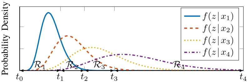
Figure 5: PDF of the receive energy per backscatter block conditioned on different reflection state.

When the threshold vector $\boldsymbol{t}\triangleq[t_{0},\ldots,t_{L}]^{\mathsf{T}}\in\mathbb{R}_{+}^{L+1}$ is given, we can formulate a Discrete Memoryless Multiple Access Channel (DMMAC) with transition probability from input $x_{m_{\mathcal{K}}}$ to output $\hat{x}_{m_{\mathcal{K}}^{\prime}}$ as

$$q(\hat{x}_{m_{\mathcal{K}}^{\prime}}|x_{m_{\mathcal{K}}})=\int_{\mathcal{R}_{m_{\mathcal{K}}^{\prime}}}f(z|x_{m_{\mathcal{K}}})\,dz.$$ (10)

The backscatter mutual information is

$$I_{\text{B}}(x_{\mathcal{K}};\hat{x}_{\mathcal{K}})=\sum_{m_{\mathcal{K}}}p(x_{m_{\mathcal{K}}})I_{\text{B}}(x_{m_{\mathcal{K}}};\hat{x}_{\mathcal{K}}),$$ (11)

where $I_{\text{B}}(x_{m_{\mathcal{K}}};\hat{x}_{\mathcal{K}})$ is the backscatter information function

$$I_{\text{B}}(x_{m_{\mathcal{K}}};\hat{x}_{\mathcal{K}})\triangleq\sum_{m_{\mathcal{K}}^{\prime}}q(\hat{x}_{m_{\mathcal{K}}^{\prime}}|x_{m_{\mathcal{K}}})\log\frac{q(\hat{x}_{m_{\mathcal{K}}^{\prime}}|x_{m_{\mathcal{K}}})}{p(\hat{x}_{m_{\mathcal{K}}^{\prime}})}.$$ (12)

Once the backscatter information is successfully decoded, the user re-encodes to recover the reflection pattern, constructs the composite channel by (4), then coherently decodes the primary link. The primary mutual information is

$$I_{\text{P}}(s;y|x_{\mathcal{K}})=\sum_{m_{\mathcal{K}}}p(x_{m_{\mathcal{K}}})I_{\text{P}}(s;y|x_{m_{\mathcal{K}}}),$$ (13)

where $I_{\text{P}}(s;y|x_{m_{\mathcal{K}}})$ is the primary information function

$$I_{\text{P}}(s;y|x_{m_{\mathcal{K}}})\triangleq\log\Bigl{(}1+\frac{\lvert\boldsymbol{h}^{\mathsf{H}}(x_{m_{\mathcal{K}}})\boldsymbol{w}\rvert^{2}}{\sigma_{v}^{2}}\Bigr{)}.$$ (14)

III Rate-Region Characterization

With a slight abuse of notation, we define the weighed sum mutual information and information function as

$$I(x_{\mathcal{K}}) \triangleq\rho I_{\text{P}}(s;y|x_{\mathcal{K}})+(1-\rho)I_{\text{B}}(x_{\mathcal{K}};\hat{x}_{\mathcal{K}}),$$ (15)

$$I(x_{m_{\mathcal{K}}}) \triangleq\rho I_{\text{P}}(s;y|x_{m_{\mathcal{K}}})+(1-\rho)I_{\text{B}}(x_{m_{\mathcal{K}}};\hat{x}_{\mathcal{K}}),$$ (16)

where $\rho\in\mathbb{I}$ is the QoS. To obtain the achievable primary-(total-)backscatter rate region, we consider the weighted sum mutual information maximization problem with independent encoding at all nodes {pk}k ∈K,w,tI(x_K) 1^T p_k=1, ∀k p_k≥0, ∀k ∥w ∥^2≤P t_l-1≤t_l, ∀l t≥0, where $\boldsymbol{p}_{k}=[p(x_{1_{k}}),\ldots,p(x_{M_{k}})]^{\mathsf{T}}\in\mathbb{I}^{M}$ is the input distribution of node $k$. Problem (12) generalizes BackCom by allowing CSI- and QoS-adaptive input distribution and decision region design. On the other hand, it also relaxes the feasible domain of discrete RIS phase shift selection problems from the vertices of $M$-dimensional probability simplex to the simplex itself. The original problem is highly non-convex and we propose a BCD algorithm that iteratively updates $\{\boldsymbol{p}_{k}\}_{k\in\mathcal{K}}$, $\boldsymbol{w}$ and $\boldsymbol{t}$.

III-A Input Distribution

For any given $\boldsymbol{w}$ and $\boldsymbol{t}$, we can formulate a DMMAC by (10) and simplify (12) to {pk}k ∈KI(x_K) (12),(12), which involves the product term (6) and is generally non-convex (unless $K=1$). Following [64], we first recast the KKT conditions to their equivalent forms, then propose a numerical solution that guarantees those conditions on the converging point of a sequence.

Proposition 1.

The KKT optimality conditions for problem (III-A) are equivalent to, $\forall k,m_{k}$,

$$I_{k}^{\star}(x_{m_{k}}) =I^{\star}(x_{\mathcal{K}}),\quad \text{if}\ p^{\star}(x_{m_{k}})>0,$$ (17a)

$$I_{k}^{\star}(x_{m_{k}}) \leq I^{\star}(x_{\mathcal{K}}),\quad \text{if}\ p^{\star}(x_{m_{k}})=0,$$ (17b)

where $I_{k}(x_{m_{k}})$ is the weighted sum marginal information

$$I_{k}(x_{m_{k}}) \triangleq\sum_{m_{\mathcal{K}\setminus\{k\}}}p(x_{m_{\mathcal{K}\setminus\{k\}}})I(x_{m_{\mathcal{K}}}).$$ (18)

Proof.

Please refer to Appendix 41. ∎

For each RIScatter node, (17a) suggests each probable state should produce the same marginal information (averaged over all states of other nodes), while (17b) suggests any state with potentially less marginal information should not be used.

Proposition 2.

For any strictly positive initializer $\{\boldsymbol{p}_{k}^{(0)}\}_{k\in\mathcal{K}}$, the KKT input probability of node $k$ at state $m_{k}$ is given by the converging point of the sequence

$$p^{(r+1)}(x_{m_{k}})=\frac{p^{(r)}(x_{m_{k}})\exp\Bigl{(}\frac{\rho}{1-\rho}I_{k}^{(r)}(x_{m_{k}})\Bigr{)}}{\sum_{m_{k}^{\prime}}p^{(r)}(x_{m_{k}^{\prime}})\exp\Bigl{(}\frac{\rho}{1-\rho}I_{k}^{(r)}(x_{m_{k}^{\prime}})\Bigr{)}},$$ (19)

where $r$ is the iteration index.

Proof.

Please refer to Appendix 51. ∎

At iteration $r+1$, the input distribution of node $k$ is updated over $\bigl{\{}\{\boldsymbol{p}_{q}^{(r+1)}\}_{q=1}^{k-1},\{\boldsymbol{p}_{q}^{(r)}\}_{q=k}^{K}\bigr{\}}$. The KKT input distribution design is summarized in Algorithm 1.

1: Input Distribution Evaluation by a Sequence

1:$K$, $N$, $\boldsymbol{h}_{\text{D}}^{\mathsf{H}}$, $\boldsymbol{H}_{\text{C}}$, $\boldsymbol{\alpha}$, $\mathcal{X}$, $\sigma_{v}^{2}$, $\rho$, $\boldsymbol{w}$, $\boldsymbol{t}$, $\epsilon$

2:$\{\boldsymbol{p}_{k}^{\star}\}_{k\in\mathcal{K}}$

3:Set $\boldsymbol{h}^{\mathsf{H}}(x_{m_{\mathcal{K}}})$, $\forall m_{\mathcal{K}}$ by (4)

4:Set $\sigma^{2}_{m_{\mathcal{K}}}$, $\forall m_{\mathcal{K}}$ by (7)

5:Set $f(z|x_{m_{\mathcal{K}}})$, $\forall m_{\mathcal{K}}$ by (8)

6:Set $q(\hat{x}_{m_{\mathcal{K}}^{\prime}}|x_{m_{\mathcal{K}}})$, $\forall m_{\mathcal{K}},m_{\mathcal{K}}^{\prime}$ by (10)

7:Initialize $r\leftarrow 0$

8:Initialize $\boldsymbol{p}_{k}^{(0)}>\boldsymbol{0}$, $\forall k$

9:Get $p^{(r)}(x_{m_{\mathcal{K}}})$, $\forall m_{\mathcal{K}}$ by (6)

10:Get $I^{(r)}(x_{m_{\mathcal{K}}})$, $\forall m_{\mathcal{K}}$ by (12), (14), (16)

11:Get $I^{(r)}_{k}(x_{m_{k}})$, $\forall k,m_{k}$ by (18)

12:Get $I^{(r)}(x_{\mathcal{K}})$ by (11), (13), (15)

13:Repeat

14:    Update $r\leftarrow r+1$

15:    Update $\boldsymbol{p}_{k}^{(r)}$, $\forall k$ by (19)

16:    Redo step 9–12

17:Until $I^{(r)}(x_{\mathcal{K}})-I^{(r-1)}(x_{\mathcal{K}})\leq\epsilon$

Remark 5.

The insufficiency of the KKT conditions for problem (III-A) implies that the proposed method may not converge to the global-optimal solution. However, simulation results in Section IV will show that the average performance gap is indistinguishable at a moderate $K$.

III-B Active Beamforming

For any given $\{\boldsymbol{p}_{k}\}_{k\in\mathcal{K}}$ and $\boldsymbol{t}$, problem (12) reduces to wI(x_K) (12), which is still non-convex due to the integration and entropy terms. Note the DMMAC $q(x_{l}|x_{m_{\mathcal{K}}})$ depends on the variance of accumulated receive energy $\sigma_{m_{\mathcal{K}}}^{2}$, which is a function of $\boldsymbol{w}$. Plugging (8) into (10), we have

$$q(x_{l}|x_{m_{\mathcal{K}}}) =\frac{\int_{{t_{l-1}}/{\sigma_{m_{\mathcal{K}}}^{2}}}^{{t_{l}}/{\sigma_{m_{\mathcal{K}}}^{2}}}z^{N-1}\exp(-z)\,dz}{(N-1)!}$$ (20)

$$=Q\Bigl{(}N,\frac{t_{l-1}}{\sigma_{m_{\mathcal{K}}}^{2}},\frac{t_{l}}{\sigma_{m_{\mathcal{K}}}^{2}}\Bigr{)},$$ (21)

where $Q(N,b_{1},b_{2})\triangleq\int_{b_{1}}^{b_{2}}z^{N-1}\exp(-z)/(N-1)!\,dz$ is the regularized incomplete Gamma function. Its series expansion is given by [65, Theorem 3]

$$Q\Bigl{(}N,\frac{t_{l-1}}{\sigma_{m_{\mathcal{K}}}^{2}},\frac{t_{l}}{\sigma_{m_{\mathcal{K}}}^{2}}\Bigr{)} =\exp\Bigl{(}-\frac{t_{l-1}}{\sigma_{m_{\mathcal{K}}}^{2}}\Bigr{)}\sum_{n=0}^{N-1}\frac{\bigl{(}\frac{t_{l-1}}{\sigma_{m_{\mathcal{K}}}^{2}}\bigr{)}^{n}}{n!}$$

$$\quad-\exp\Bigl{(}-\frac{t_{l}}{\sigma_{m_{\mathcal{K}}}^{2}}\Bigr{)}\sum_{n=0}^{N-1}\frac{\bigl{(}\frac{t_{l}}{\sigma_{m_{\mathcal{K}}}^{2}}\bigr{)}^{n}}{n!},$$ (22)

whose gradient with respect to $\boldsymbol{w}^{*}$ is

$$\nabla_{\boldsymbol{w}^{*}}Q\Bigl{(}N,\frac{t_{l-1}}{\sigma_{m_{\mathcal{K}}}^{2}},\frac{t_{l}}{\sigma_{m_{\mathcal{K}}}^{2}}\Bigr{)} =\frac{\boldsymbol{h}(x_{m_{\mathcal{K}}})\boldsymbol{h}^{\mathsf{H}}(x_{m_{\mathcal{K}}})\boldsymbol{w}}{(\sigma_{m_{\mathcal{K}}}^{2})^{2}}$$

$$\quad\times\Bigl{(}g_{m_{\mathcal{K}}}(t_{l})-g_{m_{\mathcal{K}}}(t_{l-1})\Bigr{)},$$ (23)

where

$$g_{m_{\mathcal{K}}}(t_{l})=t_{l}\exp\Bigl{(}-\frac{t_{l}}{\sigma_{m_{\mathcal{K}}}^{2}}\Bigr{)}\Bigl{(}-1+\sum_{n=1}^{N-1}\frac{\bigl{(}n-\frac{t_{l}}{\sigma_{m_{\mathcal{K}}}^{2}}\bigr{)}\bigl{(}\frac{t_{l}}{\sigma_{m_{\mathcal{K}}}^{2}}\bigr{)}^{n-1}}{n!}\Bigr{)}.$$ (24)

On top of (22) and (23), we rewrite $I(x_{\mathcal{K}})$ and $\nabla_{\boldsymbol{w}^{*}}I(x_{\mathcal{K}})$ as (25) and (26) at the end of page 25, respectively.

 

$$I(x_{\mathcal{K}})=\sum_{m_{\mathcal{K}}}p(x_{m_{\mathcal{K}}})\Biggl{(}\rho\log\Bigl{(}1+\frac{\lvert\boldsymbol{h}^{\mathsf{H}}(x_{m_{\mathcal{K}}})\boldsymbol{w}\rvert^{2}}{\sigma_{v}^{2}}\Bigr{)}+(1-\rho)\sum_{l}Q\Bigl{(}N,\frac{t_{l-1}}{\sigma_{m_{\mathcal{K}}}^{2}},\frac{t_{l}}{\sigma_{m_{\mathcal{K}}}^{2}}\Bigr{)}\log\frac{Q\Bigl{(}N,\frac{t_{l-1}}{\sigma_{m_{\mathcal{K}}}^{2}},\frac{t_{l}}{\sigma_{m_{\mathcal{K}}}^{2}}\Bigr{)}}{\sum_{m_{\mathcal{K}}^{\prime}}p(x_{m_{\mathcal{K}}^{\prime}})Q\Bigl{(}N,\frac{t_{l-1}}{\sigma_{m_{\mathcal{K}}^{\prime}}^{2}},\frac{t_{l}}{\sigma_{m_{\mathcal{K}}^{\prime}}^{2}}\Bigr{)}}\Biggr{)}$$ (25)

$$\nabla_{\boldsymbol{w}^{*}}I(x_{\mathcal{K}}) =\sum_{m_{\mathcal{K}}}p(x_{m_{\mathcal{K}}})\Biggl{(}\rho\frac{\boldsymbol{h}(x_{m_{\mathcal{K}}})\boldsymbol{h}^{\mathsf{H}}(x_{m_{\mathcal{K}}})\boldsymbol{w}}{\sigma_{m_{\mathcal{K}}}^{2}}+(1-\rho)\sum_{l}\biggl{(}\log\frac{Q\Bigl{(}N,\frac{t_{l-1}}{\sigma_{m_{\mathcal{K}}}^{2}},\frac{t_{l}}{\sigma_{m_{\mathcal{K}}}^{2}}\Bigr{)}}{\sum_{m_{\mathcal{K}}^{\prime}}p(x_{m_{\mathcal{K}}^{\prime}})Q\Bigl{(}N,\frac{t_{l-1}}{\sigma_{m_{\mathcal{K}}^{\prime}}^{2}},\frac{t_{l}}{\sigma_{m_{\mathcal{K}}^{\prime}}^{2}}\Bigr{)}}+1\biggr{)}$$

$$\qquad\times\nabla_{\boldsymbol{w}^{*}}Q\Bigl{(}N,\frac{t_{l-1}}{\sigma_{m_{\mathcal{K}}}^{2}},\frac{t_{l}}{\sigma_{m_{\mathcal{K}}}^{2}}\Bigr{)}-\frac{Q\Bigl{(}N,\frac{t_{l-1}}{\sigma_{m_{\mathcal{K}}}^{2}},\frac{t_{l}}{\sigma_{m_{\mathcal{K}}}^{2}}\Bigr{)}\sum_{m_{\mathcal{K}}^{\prime}}p(x_{m_{\mathcal{K}}^{\prime}})\nabla_{\boldsymbol{w}^{*}}Q\Bigl{(}N,\frac{t_{l-1}}{\sigma_{m_{\mathcal{K}}^{\prime}}^{2}},\frac{t_{l}}{\sigma_{m_{\mathcal{K}}^{\prime}}^{2}}\Bigr{)}}{\sum_{m_{\mathcal{K}}^{\prime}}p(x_{m_{\mathcal{K}}^{\prime}})Q\Bigl{(}N,\frac{t_{l-1}}{\sigma_{m_{\mathcal{K}}^{\prime}}^{2}},\frac{t_{l}}{\sigma_{m_{\mathcal{K}}^{\prime}}^{2}}\Bigr{)}}\Biggr{)}$$ (26)

Problem (III-B) can thus be solved by the PGA method. At iteration $r+1$, the unregulated active beamformer is updated by

$$\bar{\boldsymbol{w}}^{(r+1)}=\boldsymbol{w}^{(r)}+\gamma\nabla_{\boldsymbol{w}^{*}}I^{(r)}(x_{\mathcal{K}}),$$ (27)

where $\gamma$ is the step size (refinable by backtracking line search [66, Section 9.2]). Then, $\bar{\boldsymbol{w}}$ is projected onto the feasible domain (12) to retrieve the active beamformer

$$\boldsymbol{w}=\frac{\sqrt{P}\bar{\boldsymbol{w}}}{\max\bigl{(}\sqrt{P},\lVert\bar{\boldsymbol{w}}\rVert\bigr{)}}.$$ (28)

The PGA active beamforming design is summarized in Algorithm 2.

2: Active Beamforming Optimization by PGA

1:$Q$, $N$, $\boldsymbol{h}_{\text{D}}^{\mathsf{H}}$, $\boldsymbol{H}_{\text{C}}$, $\boldsymbol{\alpha}$, $\mathcal{X}$, $P$, $\sigma_{v}^{2}$, $\rho$, $\{\boldsymbol{p}_{k}\}_{k\in\mathcal{K}}$, $\boldsymbol{t}$, $\alpha$, $\beta$, $\gamma$, $\epsilon$

2:$\boldsymbol{w}^{\star}$

3:Set $\boldsymbol{h}^{\mathsf{H}}(x_{m_{\mathcal{K}}})$, $\forall m_{\mathcal{K}}$ by (4)

4:Set $p(x_{m_{\mathcal{K}}})$, $\forall m_{\mathcal{K}}$ by (6)

5:Initialize $r\leftarrow 0$

6:Initialize $\boldsymbol{w}^{(0)}$, $\lVert\boldsymbol{w}^{(0)}\rVert^{2}\leq P$

7:Get $(\sigma_{m_{\mathcal{K}}}^{(r)})^{2}$, $\forall m_{\mathcal{K}}$ by (7)

8:Get $Q^{(r)}\bigl{(}N,\frac{t_{l-1}}{\sigma_{m_{\mathcal{K}}}^{2}},\frac{t_{l}}{\sigma_{m_{\mathcal{K}}}^{2}}\bigr{)}$, $\forall m_{\mathcal{K}},l$ by (22)

9:Get $I^{(r)}(x_{\mathcal{K}})$ by (25)

10:Get $\nabla_{\boldsymbol{w}^{*}}Q^{(r)}\bigl{(}N,\frac{t_{l-1}}{\sigma_{m_{\mathcal{K}}}^{2}},\frac{t_{l}}{\sigma_{m_{\mathcal{K}}}^{2}}\bigr{)}$, $\forall m_{\mathcal{K}},l$ by (23)

11:Get $\nabla_{\boldsymbol{w}^{*}}I^{(r)}(x_{\mathcal{K}})$ by (26)

12:Repeat

13:    Update $r\leftarrow r+1$

14:    Update $\gamma^{(r)}\leftarrow\gamma$

15:    Update $\bar{\boldsymbol{w}}^{(r)}$ by (27)

16:    Update $\boldsymbol{w}^{(r)}$ by (28)

17:    Redo step 7–9

18:    While $I^{(r)}(x_{\mathcal{K}})<I^{(r-1)}(x_{\mathcal{K}})+\alpha\gamma\lVert\nabla_{\boldsymbol{w}^{*}}I^{(r-1)}(x_{\mathcal{K}})\rVert^{2}$ 

19:         Set $\gamma^{(r)}\leftarrow\beta\gamma^{(r)}$

20:         Redo step 15–17

21:    End While

22:    Redo step 10, 11

23:Until $\lVert\boldsymbol{w}^{(r)}-\boldsymbol{w}^{(r-1)}\rVert\leq\epsilon$

III-C Decision Threshold

For any given $\{\boldsymbol{p}_{k}\}_{k\in\mathcal{K}}$ and $\boldsymbol{w}$, problem (12) reduces to tI(x_K) (12),(12), which is still non-convex since $\boldsymbol{t}$ appears on the limits of integration (10). Instead of solving it directly, we constrain the feasible domain from continuous space $\mathbb{R}_{+}^{L+1}$ to discrete candidates (i.e., fine-grained energy levels) $\mathcal{T}^{L+1}$. As shown in Fig. 6, the decision regions are formulated by grouping adjacent energy bins.

Figure 6: The thresholds are chosen from fine-grained candidates instead of the continuous space. Each decision region consists of at least one bin.

Remark 6.

The design of the energy detector does not affect the primary achievable rate, since the composite channel (4) can always be determined after backscatter decoding and re-encoding. This implies that any thresholding maximizing the total backscatter rate is optimal for problem (III-C).

Remark 7.

In terms of total backscatter rate, the nodes can be viewed as an augmented source, and problem (III-C) becomes the rate-optimal quantizer design for DMTC.

Thanks to Remark 6 and 7, problem (III-C) can be recast as t ∈TL+1I_B(x_K;^x_K) (12), whose global optimal solution has been obtained in recent works. [67] started from the quadrangle inequality and proposed a Dynamic Programming (DP) method accelerated by the Shor-Moran-Aggarwal-Wilber-Klawe (SMAWK) algorithm with computational complexity $\mathcal{O}\bigl{(}L^{2}(\mathrm{card}(\mathcal{T})-L)\bigr{)}$. On the other hand, [68] started from the optimality condition for three neighbor thresholds and presented a traverse-then-bisect algorithm with complexity $\mathcal{O}\bigl{(}\mathrm{card}(\mathcal{T})L\log(\mathrm{card}(\mathcal{T})L)\bigr{)}$. In Section IV, both schemes will be compared with the Maximum-Likelihood (ML) scheme [60]

$$t_{l}^{\text{\lx@glossaries@gls@link{main}{ml}{\leavevmode ML}}}=N\frac{\sigma_{l-1}^{2}\sigma_{l}^{2}}{\sigma_{l-1}^{2}-\sigma_{l}^{2}}\log\frac{\sigma_{l-1}^{2}}{\sigma_{l}^{2}},\quad l\in\mathcal{L}\setminus\{L\},$$ (29)

which is suboptimal for problem (III-C) unless all nodes are with equiprobable inputs.

IV Simulation Results

In this section, we provide numerical results to evaluate the proposed algorithms. We assume the AP-user distance is 10m and at least one RIScatter nodes are randomly dropped in a disk centered at the user with radius $r$. The AP is with maximum average transmit power $P=\qty{36}{dBm}$ and all nodes employs $M$-QAM with $\alpha=0.5$. For all channels involved, we consider a distance-dependent path loss model

$$L(d)=L_{0}\biggl{(}\frac{d_{0}}{d}\biggr{)}^{\gamma},$$ (30)

together with a Rician fading model

$$\boldsymbol{H}=\sqrt{\frac{\kappa}{1+\kappa}}\bar{\boldsymbol{H}}+\sqrt{\frac{1}{1+\kappa}}\tilde{\boldsymbol{H}},$$ (31)

where $d$ is the transmission distance, $L_{0}=-\qty{30}{dB}$ is the reference path loss at $d_{0}=\qty{1}{m}$, $\kappa$ is the Rician K-factor, $\bar{\boldsymbol{H}}$ is the deterministic line-of-sight component with unit-magnitude entries, and $\tilde{\boldsymbol{H}}$ is the Rayleigh fading component with standard independent and identically distributed (i.i.d.) CSCG entries. We choose $\gamma_{\text{D}}=2.6$, $\gamma_{\text{F}}=2.4$, $\gamma_{\text{B}}=2$, and $\kappa_{\text{D}}=\kappa_{\text{F}}=\kappa_{\text{B}}=5$ for direct, forward and backward links. The finite decision threshold domain $\mathcal{T}$ is obtained by $b$-bit uniform discretization over the critical interval defined by the $1-\varepsilon$ confidence bounds of edge hypotheses (i.e., lower bound of $x_{1}$ and upper bound of $x_{L}$). We set $b=9$ and $\varepsilon=${10}^{-3}$$. All achievable rate regions are averaged over ${10}^{3}$ channel realizations.

IV-A Evaluation of Proposed Algorithms

IV-A1 Initialization

To characterize the achievable rate region, we progressively obtain all boundary points by successively increasing $\rho$ and solving problem (12). For $\rho=0$ where the backscatter link is prioritized, we initialize Algorithm 1 and 2 by uniform input distribution and Maximum Ratio Transmission (MRT) towards the sum cascaded channel $\sum_{k}\boldsymbol{h}_{\text{C},k}^{\mathsf{H}}$, respectively. At the following points, both algorithms are initialized by the solutions at the previous point.

IV-A2 Convergence

Figure 7: Typical convergence curves at $\rho=0$ for $Q=4$, $K=8$, $M=2$, $N=20$, $\sigma_{v}^{2}=\qty{-40}{dBm}$ and $r=\qty{2}{m}$.

The BCD algorithm is convergent for problem (12) since the input distribution and active beamforming subproblems converge and the thresholding subproblem attains global optimality. In company with BCD, we also plotted the convergence results of KKT and PGA algorithms in Fig. 7 to show how much performance is gained by solving each subproblem. It is observed that Algorithm 1 and 2 take around $100$ and $10$ iterations to converge, respectively. Overall, the BCD algorithm requires at most $5$ iterations to converge. As $\rho$ increases (not presented here), the convergence of all three algorithms are much faster thanks to the progressive initialization.

IV-B Comparison of Scattering Applications

On top of the setup in Fig. 4, we consider RIScatter and the following benchmark applications:

• Legacy: Legacy transmission without scatter nodes.

• BBC: The primary signal is CW and the receive signal is

  $$y^{\text{\lx@glossaries@gls@link{main}{bbc}{\leavevmode BBC}}}[n]=\Bigl{(}\boldsymbol{h}_{\text{D}}^{\mathsf{H}}+\sum_{k}\alpha_{k}\boldsymbol{h}_{\text{C},k}^{\mathsf{H}}x_{k}\Bigr{)}\boldsymbol{w}+v[n].$$ (32)

  The total backscatter rate approaches $K\log M$ when $N$ is sufficiently large.

• AmBC: The user decodes each link independently and semi-coherently while treating the other as interference. The primary achievable rate is approximately

  $$I_{\text{P}}^{\text{\lx@glossaries@gls@link{main}{ambc}{\leavevmode AmBC}}}(s;y)\approx\log\Bigl{(}1+\frac{\lvert\boldsymbol{h}_{\text{D}}^{\mathsf{H}}\boldsymbol{w}\rvert^{2}}{\sum_{k}\lvert\alpha_{k}\boldsymbol{h}_{\text{C},k}^{\mathsf{H}}\boldsymbol{w}\rvert^{2}+\sigma_{v}^{2}}\Bigr{)},$$ (33)

  while the total backscatter rate follows (11) with uniform input distribution.

• SR: For a sufficiently large $N$, the average primary rate under semi-coherent detection asymptotically approaches (13) with uniform input distribution [15]. When $s[n]$ is successfully decoded and the direct interference $\boldsymbol{h}_{\text{D}}^{\mathsf{H}}\boldsymbol{w}s[n]$ is perfectly cancelled, the intermediate signal is

  $$\hat{y}^{\text{\lx@glossaries@gls@link{main}{sr}{\leavevmode SR}}}[n]=\sum_{k}\alpha_{k}\boldsymbol{h}_{\text{C},k}^{\mathsf{H}}x_{k}\boldsymbol{w}s[n]+v[n].$$ (34)

  The total backscatter rate approaches $K\log M$.

• RIS: The reflection pattern is deterministic and the total backscatter rate is zero. The primary achievable rate is a special case of (13)

  $$I_{\text{P}}^{\text{\lx@glossaries@gls@link{main}{ris}{\leavevmode RIS}}}(s;y|x_{\mathcal{K}})=I_{\text{P}}(s;y|x_{m_{\mathcal{K}}^{\star}})=\log\Bigl{(}1+\frac{\lvert\boldsymbol{h}^{\mathsf{H}}(x_{m_{\mathcal{K}}^{\star}})\boldsymbol{w}\rvert^{2}}{\sigma_{v}^{2}}\Bigr{)},$$ (35)

  where $m_{\mathcal{K}}^{\star}=\arg\max_{m_{\mathcal{K}}}I_{\text{P}}^{\text{\lx@glossaries@gls@link{main}{ris}{\leavevmode RIS}}}(s;y|x_{m_{\mathcal{K}}})$.

Figure 8: Typical achievable rate region/points of scattering applications for $Q=1$, $K=1$, $M=4$, $N=${10}^{3}$$, $\sigma_{v}^{2}=\qty{-40}{dBm}$ and $r=\qty{2}{m}$.

Fig. 8 compares the typical achievable rate region/points of RIScatter and those strategies. First, we observe BBC and SR achieve the best backscatter performance thanks to the coherent decoding. For SR, this comes with the cost of $N$ re-encoding, precoding, subtraction together with a time-domain MRC per backscatter symbol. Since SR requires a very large $N$ to guarantee the primary rate, the signal processing cost at the receiver can be prohibitive, and the backscatter throughput can be severely constrained. Second, the average primary rate slightly decreases/increases in the presence of a AmBC/RIS node, and the benefit of SR is not obvious. This is because the cascaded channel is around 25dB weaker than the direct channel. Here, RIS ensures a constructive superposition of the direct and scattered components, while SR only creates a quasi-static rich-scattering environment that marginally enhances the average primary rate. When $N$ is moderate, the randomly scattered signals should be modelled as interference rather than stable multipath, and the SR point should move vertically towards the AmBC point. Third, RIScatter enables a flexible primary-backscatter tradeoff with adaptive input distribution design. In terms of maximum primary achievable rate, RIScatter coincides with RIS and outperforms the others by using the static reflection pattern that maximizes the primary SNR all the time. On the other hand, its maximum backscatter achievable rate is higher than that of AmBC. This is because the adaptive channel coding of RIScatter outperforms the equiprobable inputs of AmBC, especially at the low backscatter SNR caused by double fading. When multiple antenna is available at the AP, active beamforming can be optimized for RIScatter nodes and the advantage over AmBC should be more prominent.

IV-C Input Distribution under Different QoS

Figure 9: Typical RIScatter reflection state distribution at different $\rho$ for $Q=1$, $K=1$, $M=4$, $N=20$, $\sigma_{v}^{2}=\qty{-40}{dBm}$ and $r=\qty{2}{m}$.

The objective is to demonstrate RIScatter nodes can leverage CSI- and QoS-adaptive input distribution design to balance backscatter modulation and passive beamforming. For one RIScatter node with $M=4$, we evaluate the KKT input distribution at different QoS and present the result in Fig. 9. At $\rho=0$ where the backscatter performance is prioritized, the optimal input distribution is $0$ on two states and nearly uniform on the other two. This is inline with Shannon’s observation that binary antipodal inputs is good enough for channel capacity at low SNR [69]. When the scattered signal is relatively weak, the conditional energy PDF under different hypotheses can be closely spaced as in Fig. 5. The extreme states producing the lowest/highest energy are always assigned with non-zero probability, while the middles cannot provide enough energy diversity and end up unused. At $\rho=1$ where the primary link is prioritized, the optimal input distribution is $[0,0,1,0]^{\mathsf{T}}$ since state 3 provides higher primary SNR than other states. That is, the reflection pattern becomes deterministic and the RIScatter node boils down to a static discrete RIS element. Increasing $\rho$ from $0$ to $1$ creates a smooth transition from backscatter modulation to passive beamforming, suggesting RIScatter unifies BackCom and RIS from a probabilistic perspective.

IV-D Rate Region by Different Schemes

(a) Input Distribution, $Q=1$

(b) Active Beamforming, $Q=4$

(c) Decision Threshold, $Q=4$

Figure 10: Average primary-total-backscatter rate regions by different input distribution, active beamforming, and decision threshold schemes for $K=2$, $M=4$, $N=20$, $\sigma_{v}^{2}=\qty{-40}{dBm}$ and $r=\qty{2}{m}$.

IV-D1 Input Distribution

We compare these input distribution designs for problem (III-A):

• Cooperation: Joint encoding using a joint probability array $p(x_{m_{\mathcal{K}}})$ with $M^{K}$ entries by Algorithm 1;

• Exhaustion: Exhaustive search over the $M$-dimensional probability simplex with resolution $\Delta p=${10}^{-2}$$;

• KKT: Solution by Algorithm 1;

• Equiprobable: Uniform input distribution.

We also consider these independent distribution recovery methods from the joint probability array:

• Marginalization: Marginal probability distributions;

• Decomposition: Normalized rank-$1$ Canonical Polyadic (CP) decomposed tensors by Tensor Toolbox [70];

• Randomization: Gaussian randomization with the guidance of correlation matrix [71].

Fig. LABEL:sub@fg:region_distribution shows their average achievable rate regions. Cooperation achieves the outer bound of all schemes, but joint encoding over passive devices may incur additional hardware cost. Besides, the average rate performance of Exhaustion and KKT completely coincide with each other when $K=2$. This confirms Remark 5 that the KKT input distribution can be good enough when $K$ is moderate. Equiprobable experiences minor backscatter and major primary rate losses without exploiting CSI and QoS, and those gaps should be larger when $M$ or $K$ increases. Marginalization provides a close performance to KKT, but Randomization and Decomposition fail our expectations for most channel realizations. Those observations emphasize the importance of adaptive RIScatter encoding and demonstrate the advantage of the proposed KKT input distribution design.

IV-D2 Active Beamforming

We consider three typical active beamforming schemes for problem (III-B):

• PGA: Solution by Algorithm 2;

• E-MRT: MRT towards the ergodic composite channel $\sum_{m_{\mathcal{K}}}p(x_{m_{\mathcal{K}}})\boldsymbol{h}^{\mathsf{H}}(x_{m_{\mathcal{K}}})$;

• D-MRT: MRT towards the direct channel $\boldsymbol{h}_{\text{D}}^{\mathsf{H}}$.

Fig. LABEL:sub@fg:region_beamforming presents the average achievable rate regions for those schemes. In the low-$\rho$ regime, the proposed PGA beamformer significantly outperforms both MRT schemes in terms of total backscatter rate. This is because the semi-coherent backscatter decoding relies on the relative energy difference under different backscatter symbol tuples. Such an energy diversity is enhanced by PGA that effectively exploits backscatter constellation and input distribution knowledge rather than simply maximizes the channel strength. As $\rho$ increases, the primary SNR outweighs the backscatter energy difference in (25), and PGA beamformer approaches E-MRT. At $\rho=1$, both PGA and E-MRT boil down to MRT towards the strongest composite channel. The difference between E-MRT and D-MRT is insignificant when RIScatter nodes are dispersed. Those observations confirm that the proposed PGA active beamforming design can exploit the CSI, QoS, and backscatter constellation to enlarge the achievable rate region.

IV-D3 Decision Threshold

We evaluate the following decision threshold strategies for problem (7):

• DP: Benchmark DP method for sequential quantizer [67];

• SMAWK: DP accelerated by the SMAWK algorithm [67];

• Bisection: The traverse-then-bisect algorithm [68];

• ML: Maximum likelihood detector (29) [60].

Fig. LABEL:sub@fg:region_threshold reveals the average achievable rate region for those strategies. The distribution-aware schemes DP, SMAWK and Bisection ensure higher total backscatter rate than ML. This is because the total backscatter rate (11) is a function of both input distribution and decision regions, and the rate-optimal thresholding depends heavily on the input distribution. For example, the backscatter symbol tuples with zero input probability should be assigned with empty decision regions, in order to increase the success detection rates of other hypotheses. It highlights the importance of joint input distribution and decision threshold design in rate maximization problems.

IV-E Rate Region under Different Configurations

(a) RIScatter Nodes

(b) Reflection States

(c) Transmit Antennas

(d) Spreading Factor

(e) Average Noise Power

(f) Imperfect CSI

(g) Primary SNR

(h) Backscatter SNR

Figure 11: Average primary-total-backscatter rate regions for different system configurations.

In this study, we choose $Q=4$, $K=8$, $M=2$, $N=20$, $\sigma_{v}^{2}=\qty{-40}{dBm}$ and $r=\qty{2}{m}$ as a reference, unless otherwise specified.

IV-E1 Number of Nodes

Fig. LABEL:sub@fg:region_tags reveals how the number RIScatter nodes $K$ influences the primary-backscatter tradeoff. Interestingly, we observe that increasing $K$ has a larger benefit on the total backscatter rate than primary. This is because each RIScatter node not only affects the primary SNR but also influences the relative energy difference that other nodes can make. To maximize the total backscatter rate, some nodes closer to the user may need to sacrifice their own rate and use the state that minimizes the composite channel strength, in order to increase the backscatter rate of other nodes. This accounts for the significant primary rate decrease in the low-$\rho$ regime. On the other hand, when the primary link is prioritized, the RIScatter nodes boil down to RIS elements and enjoy a passive array gain of $K^{2}$.

IV-E2 Number of States

Fig. LABEL:sub@fg:region_states shows the relationship between the available reflection states (i.e., QAM order) $M$ and the achievable rate region when $K=1$. We notice that increasing the reflection states has a marginal effect on the primary rate but significantly improves the backscatter rate. This is because the maximum amplitude normalized-QAM (2) involves more weak reflection points as $M$ increases. It enhances the receive energy diversity but cannot provide enough phase shift resolution with maximum reflection.

IV-E3 Number of Transmit Antennas

Fig. LABEL:sub@fg:region_txs illustrates the impact of transmit antennas $Q$ on the average performance. As $Q$ increases, more scattered paths become available and the channel diversity can be better exploited to improve the primary-backscatter tradeoff. It emphasizes the importance of multi-antenna RIScatter systems and demonstrate the effectiveness of the proposed PGA design.

IV-E4 Spreading factor

Fig. LABEL:sub@fg:region_duration shows how the spreading factor $N$ affects the achievable rate region. Using a very large $N$ (as in the case of SR) can severely constrain the backscatter throughput, since the gain in energy certainty (by the law of large numbers) cannot withstand the loss in the gross rate. As $N\to\infty$, RIScatter nodes boil down to static RIS elements and the total backscatter rate approaches $0$. On the other hand, when $N$ is too small, the DMMAC (10) becomes unreliable and energy detection is error-prone. It explains the observation that $N=10$ provides lower backscatter throughput than $N=20$. Therefore, we conclude the spreading factor $N$ should be carefully designed over multiple factors (e.g., primary and backscatter SNR, data rate requirements, load switching speed at the nodes, and signal processing capability at the user).

IV-E5 Average Noise Power

Fig. LABEL:sub@fg:region_noise depicts the impact of average noise power $\sigma_{v}^{2}$ on average rate regions. Note that the noise influences both primary and backscatter SNR. When $\sigma_{v}^{2}$ relatively high, one can choose a larger $N$ to improve the SNR of energy detection.

IV-E6 Imperfect CSI

Due to the lack of RF chains at RIScatter nodes, fast and accurate acquisition of the cascaded CSI can be challenging, especially when the backscatter SNR is weak or the number of nodes is large. We consider an imperfect CSI model, where the cascaded channel of node $k$ is estimated as

$$\hat{\boldsymbol{h}}_{\text{C},k}=\boldsymbol{h}_{\text{C},k}+\tilde{\boldsymbol{h}}_{\text{C},k},$$ (36)

$\tilde{\boldsymbol{h}}_{\text{C},k}$ is the estimation error with entries following i.i.d. CSCG distribution $\mathcal{CN}(0,\iota\Lambda_{\text{C}})$, $\iota$ is the relative estimation error, and $\Lambda_{\text{C}}$ is the cascaded path loss. In Fig. LABEL:sub@fg:region_csi, it is observed that the channel estimation error mainly affects the backscatter rate. When $\iota$ increases from $0$ to $0.2$, the maximum total backscatter rate decreases by 20. This is because the energy detector is sensitive to the DMMAC (10) and thus the estimation of the cascaded channel. On the other hand, a small estimation error may be insufficient to change the optimal passive beamforming state and the primary rate is almost unchanged.

IV-E7 Primary SNR

The backscatter SNR is fixed to 0dB with $Q=1$ in this study. Interestingly, Fig. LABEL:sub@fg:region_snr_primary shows that increasing the primary SNR can improve the primary rate but degrade the backscatter rate. The reason is that the relative strength of the scattered signal compared to the direct signal is weakened, such that the nodes cannot make enough difference to the energy detector. This, together with Fig. LABEL:sub@fg:region_beamforming and LABEL:sub@fg:region_tags, emphasizes the importance of balancing the primary and backscatter SNR in the design of active-passive coexisting networks.

IV-E8 Backscatter SNR

The primary SNR is fixed to 20dB with $Q=1$ in this study. Fig. LABEL:sub@fg:region_snr_backscatter shows that the primary and backscatter rates are both improved when the backscatter SNR increases. This motivates one to use high-efficiency or semi-passive RIScatter nodes to improve the overall performance. In a multi-user RIScatter network, each node may be assigned to the nearest user to guarantee uniformly good performance for both links.

V Conclusion

This paper introduced RIScatter as a novel scatter protocol that bridges backscatter modulation and passive beamforming. Starting from scattering principles, we showed how RIScatter nodes generalize information nodes of BackCom and reflect elements of RIS, how they can be built over existing passive scatter devices, and how they simultaneously encode self information and assist legacy transmission. We also proposed a practical SIC-free receiver that exploits the properties of active-passive coexisting networks to benefit both subsystems. The achievable primary-total-backscatter rate region was then studied for a single-user multi-node RIScatter network, where the input distribution, active beamforming, and decision thresholds are iteratively updated. Numerical results validated the proposed algorithms and emphasized the importance of adaptive input distribution and cooperative receiver design.

To support massive RIScatter networks with large number of nodes and states, one possible future direction is to consider backscatter detection over the received signal domain rather than energy domain, where multi-antenna [72] and learning-based approaches can be promising. Another interesting question is how to design RIScatter nodes and receivers in a multi-user system to fully exploit the dynamic passive beamforming that naturally origins from backscatter modulation.

-A Proof of Proposition 1

Denote the Lagrange multipliers associated with (12) and (12) as $\{\nu_{k}\}_{k\in\mathcal{K}}$ and $\{\lambda_{m_{k}}\}_{k\in\mathcal{K},m_{k}\in\mathcal{M}}$, respectively. The Lagrangian function of problem (III-A) is

$$L(p,\nu,\lambda)=I(x_{\mathcal{K}})+\sum_{k}\nu_{k}\Bigl{(}\sum_{m_{k}}p(x_{m_{k}})-1\Bigr{)}+\sum_{k,m_{k}}\lambda_{m_{k}}p(x_{m_{k}}),$$ (37)

and the KKT conditions are, $\forall k,m_{k}$,

$$I_{k}^{\star}(x_{m_{k}})-(1-\rho)+\nu_{k}^{\star}+\lambda_{m_{k}}^{\star}=0,$$ (38a)

$$\lambda_{m_{k}}^{\star}=0,\quad\text{if}\ p^{\star}(x_{m_{k}})>0,$$ (38b)

$$\lambda_{m_{k}}^{\star}\geq 0,\quad\text{if}\ p^{\star}(x_{m_{k}})=0.$$ (38c)

Plugging (38b) and (38c) into (38a) yields

$$I_{k}^{\star}(x_{m_{k}}) =1-\rho-\nu_{k}^{\star},\quad \text{if}\ p^{\star}(x_{m_{k}})>0,$$ (39a)

$$I_{k}^{\star}(x_{m_{k}}) \leq 1-\rho-\nu_{k}^{\star},\quad \text{if}\ p^{\star}(x_{m_{k}})=0,$$ (39b)

such that

$$\sum_{m_{k}}p^{\star}(x_{m_{k}})I_{k}^{\star}(x_{m_{k}})=1-\rho-\nu_{k}^{\star}.$$ (40)

On the other hand, by definition (18) we have

$$\sum_{m_{k}}p^{\star}(x_{m_{k}})I_{k}^{\star}(x_{m_{k}})=I^{\star}(x_{\mathcal{K}}),$$ (41)

where the right-hand side is irrelevant to $k$. (39), (40), and (41) together complete the proof.

-B Proof of Proposition 2

We first prove sequence (19) is non-decreasing in weighted sum mutual information. Let $p(x_{m_{\mathcal{K}}})=\prod_{q\in\mathcal{K}}p(x_{m_{q}})$ and $p^{\prime}(x_{m_{\mathcal{K}}})=p^{\prime}(x_{m_{k}})\prod_{q\in\mathcal{K}\setminus\{k\}}p(x_{m_{q}})$ be two distributions potentially different at $x_{m_{k}}$, and $J\bigl{(}p(x_{m_{\mathcal{K}}}),p^{\prime}(x_{m_{\mathcal{K}}})\bigr{)}$ be a joint function defined in (42) at the end of page 42.

 

$$J\bigl{(}p(x_{m_{\mathcal{K}}}),p^{\prime}(x_{m_{\mathcal{K}}})\bigr{)}\triangleq\sum_{m_{\mathcal{K}}}p(x_{m_{\mathcal{K}}})\Biggl{(}\rho\log\Bigl{(}1+\frac{\lvert\boldsymbol{h}^{\mathsf{H}}(x_{m_{\mathcal{K}}})\boldsymbol{w}\rvert^{2}}{\sigma_{v}^{2}}\Bigr{)}+(1-\rho)\sum_{m_{\mathcal{K}}^{\prime}}q(\hat{x}_{m_{\mathcal{K}}^{\prime}}|x_{m_{\mathcal{K}}})\log\frac{q(\hat{x}_{m_{\mathcal{K}}^{\prime}}|x_{m_{\mathcal{K}}})p^{\prime}(x_{m_{\mathcal{K}}})}{p^{\prime}(\hat{x}_{m_{\mathcal{K}}^{\prime}})p(x_{m_{\mathcal{K}}})}\Biggr{)}.$$ (42)

It is straightforward to verify $J\bigl{(}p(x_{m_{\mathcal{K}}}),p(x_{m_{\mathcal{K}}})\bigr{)}=I(x_{\mathcal{K}})$ and $J\bigl{(}p(x_{m_{\mathcal{K}}}),p^{\prime}(x_{m_{\mathcal{K}}})\bigr{)}$ is a concave function for a given $p^{\prime}(x_{m_{\mathcal{K}}})$. Setting $\nabla_{p(x_{m_{k}})}J\bigl{(}p(x_{m_{\mathcal{K}}}),p^{\prime}(x_{m_{\mathcal{K}}})\bigr{)}=0$ yields

$$S_{k}^{\prime}(x_{m_{k}})-S_{k}^{\prime}(x_{i_{k}})+(1-\rho)\log\frac{p(x_{i_{k}})}{p^{\star}(x_{m_{k}})}=0,$$ (43)

where $i_{k}\neq m_{k}$ is the reference state and

$$S_{k}^{\prime}(x_{m_{k}}) \triangleq I_{k}^{\prime}(x_{m_{k}})+(1-\rho)\sum_{m_{\mathcal{K}\setminus\{k\}}}p(x_{m_{\mathcal{K}\setminus\{k\}}})$$

$$\quad\times\sum_{m_{\mathcal{K}}^{\prime}}q(\hat{x}_{m_{\mathcal{K}}^{\prime}}|x_{m_{\mathcal{K}}})\log p^{\prime}(x_{m_{\mathcal{K}}}).$$ (44)

Evidently, $\forall m_{k}\neq i_{k}$, (43) boils down to

$$p^{\star}(x_{m_{k}})=\frac{p^{\prime}(x_{m_{k}})\exp\Bigl{(}\frac{\rho}{1-\rho}I_{k}^{\prime}(x_{m_{k}})\Bigr{)}}{\sum_{m_{k}^{\prime}}p^{\prime}(x_{m_{k}^{\prime}})\exp\Bigl{(}\frac{\rho}{1-\rho}I_{k}^{\prime}(x_{m_{k}^{\prime}})\Bigr{)}}.$$ (45)

Since $p(x_{i_{k}})=1-\sum_{m_{k}\neq i_{k}}p^{\star}(x_{m_{k}})$ has exactly the same form as (45), the choice of reference does not matter and (45) is optimal $\forall m_{k}\in\mathcal{M}$. That is, for a fixed $p^{\prime}(x_{m_{\mathcal{K}}})$, (45) ensures

$$J\bigl{(}p(x_{m_{\mathcal{K}}}),p^{\prime}(x_{m_{\mathcal{K}}})\bigr{)}\geq I^{\prime}(x_{\mathcal{K}}).$$ (46)

On the other hand, we notice

$$I(x_{\mathcal{K}})-J\bigl{(}p(x_{m_{\mathcal{K}}}),p^{\prime}(x_{m_{\mathcal{K}}})\bigr{)}$$

$$=(1-\rho)\sum_{m_{k}}\frac{p^{\prime}(x_{m_{k}})f_{k}^{\prime}(x_{m_{k}})}{\sum_{m_{k}^{\prime}}p^{\prime}(x_{m_{k}^{\prime}})f_{k}^{\prime}(x_{m_{k}^{\prime}})}\sum_{m_{\mathcal{K}}^{\prime\prime}}q(\hat{x}_{m_{\mathcal{K}}^{\prime\prime}}|x_{m_{k}})$$

$$\quad\times\log\frac{\sum_{m_{k}^{\prime}}p^{\prime}(x_{m_{k}^{\prime}})q(\hat{x}_{m_{\mathcal{K}}^{\prime\prime}}|x_{m_{k}^{\prime}})f_{k}^{\prime}(x_{m_{k}})}{\sum_{m_{k}^{\prime}}p^{\prime}(x_{m_{k}^{\prime}})q(\hat{x}_{m_{\mathcal{K}}^{\prime\prime}}|x_{m_{k}^{\prime}})f_{k}^{\prime}(x_{m_{k}^{\prime}})}$$ (47a)

$$\geq(1-\rho)\sum_{m_{k}}\frac{p^{\prime}(x_{m_{k}})f_{k}^{\prime}(x_{m_{k}})}{\sum_{m_{k}^{\prime}}p^{\prime}(x_{m_{k}^{\prime}})f_{k}^{\prime}(x_{m_{k}^{\prime}})}\sum_{m_{\mathcal{K}}^{\prime\prime}}q(\hat{x}_{m_{\mathcal{K}}^{\prime\prime}}|x_{m_{k}})$$

$$\quad\times\Biggl{(}1-\frac{\sum_{m_{k}^{\prime}}p^{\prime}(x_{m_{k}^{\prime}})q(\hat{x}_{m_{\mathcal{K}}^{\prime\prime}}|x_{m_{k}^{\prime}})f_{k}^{\prime}(x_{m_{k}^{\prime}})}{\sum_{m_{k}^{\prime}}p^{\prime}(x_{m_{k}^{\prime}})q(\hat{x}_{m_{\mathcal{K}}^{\prime\prime}}|x_{m_{k}^{\prime}})f_{k}^{\prime}(x_{m_{k}})}\Biggr{)}$$ (47b)

$$=(1-\rho)\Biggl{(}1-\sum_{m_{k}}\frac{p^{\prime}(x_{m_{k}})\cancel{f_{k}^{\prime}(x_{m_{k}})}}{\sum_{m_{k}^{\prime}}p^{\prime}(x_{m_{k}^{\prime}})f_{k}^{\prime}(x_{m_{k}^{\prime}})}\sum_{m_{\mathcal{K}}^{\prime\prime}}q(\hat{x}_{m_{\mathcal{K}}^{\prime\prime}}|x_{m_{k}})$$

$$\quad\times\frac{\sum_{m_{k}^{\prime}}p^{\prime}(x_{m_{k}^{\prime}})q(\hat{x}_{m_{\mathcal{K}}^{\prime\prime}}|x_{m_{k}^{\prime}})f_{k}^{\prime}(x_{m_{k}^{\prime}})}{\sum_{m_{k}^{\prime}}p^{\prime}(x_{m_{k}^{\prime}})q(\hat{x}_{m_{\mathcal{K}}^{\prime\prime}}|x_{m_{k}^{\prime}})\cancel{f_{k}^{\prime}(x_{m_{k}})}}\Biggr{)}$$ (47c)

$$=(1-\rho)\Biggl{(}1-\sum_{m_{\mathcal{K}}^{\prime\prime}}\frac{\cancel{\sum_{m_{k}}p^{\prime}(x_{m_{k}})q(\hat{x}_{m_{\mathcal{K}}^{\prime\prime}}|x_{m_{k}})}}{\sum_{m_{k}^{\prime}}p^{\prime}(x_{m_{k}^{\prime}})f_{k}^{\prime}(x_{m_{k}^{\prime}})}$$

$$\quad\times\frac{\sum_{m_{k}^{\prime}}p^{\prime}(x_{m_{k}^{\prime}})q(\hat{x}_{m_{\mathcal{K}}^{\prime\prime}}|x_{m_{k}^{\prime}})f_{k}^{\prime}(x_{m_{k}^{\prime}})}{\cancel{\sum_{m_{k}^{\prime}}p^{\prime}(x_{m_{k}^{\prime}})q(\hat{x}_{m_{\mathcal{K}}^{\prime\prime}}|x_{m_{k}^{\prime}})}}\Biggr{)}$$ (47d)

$$=(1-\rho)\Biggl{(}1-\frac{\sum_{m_{k}^{\prime}}p^{\prime}(x_{m_{k}^{\prime}})f_{k}^{\prime}(x_{m_{k}^{\prime}})\sum_{m_{\mathcal{K}}^{\prime\prime}}q(\hat{x}_{m_{\mathcal{K}}^{\prime\prime}}|x_{m_{k}^{\prime}})}{\sum_{m_{k}^{\prime}}p^{\prime}(x_{m_{k}^{\prime}})f_{k}^{\prime}(x_{m_{k}^{\prime}})}\Biggr{)}$$

$$=0,$$ (47e)

where $f_{k}^{\prime}(x_{m_{k}})\triangleq\exp\bigl{(}\frac{\rho}{1-\rho}I_{k}^{\prime}(x_{m_{k}})\bigr{)}$ and the equality holds if and only if $p(x_{m_{\mathcal{K}}})$ and $p^{\prime}(x_{m_{\mathcal{K}}})$ equals (i.e., (45) converges). (46) and (47) together imply $I(x_{\mathcal{K}})\geq I^{\prime}(x_{\mathcal{K}})$. Since mutual information is bounded above, we conclude the sequence (19) is non-decreasing and convergent.

Next, we prove any converging point of sequence (19), denoted as $p^{\star}(x_{m_{k}})$, fulfills the KKT conditions (17). Let

$$D^{(r)}(x_{m_{k}})\triangleq\frac{p^{(r+1)}(x_{m_{k}})}{p^{(r)}(x_{m_{k}})}=\frac{f_{k}^{(r)}(x_{m_{k}})}{\sum_{m_{k}^{\prime}}p^{(r)}(x_{m_{k}^{\prime}})f_{k}^{(r)}(x_{m_{k}^{\prime}})}.$$ (48)

As sequence (19) is convergent, any state with $p^{\star}(x_{m_{k}})>0$ need to satisfy $D^{\star}(x_{m_{k}})\triangleq\lim_{r\to\infty}D^{(r)}(x_{m_{k}})=1$, namely

$$I_{k}^{\star}(x_{m_{k}})=\frac{1-\rho}{\rho}\log\sum_{m_{k}^{\prime}}p^{\star}(x_{m_{k}^{\prime}})\exp\Bigl{(}\frac{\rho}{1-\rho}I_{k}^{\star}(x_{m_{k}^{\prime}})\Bigr{)}.$$ (49)

The right-hand side is a constant for node $k$ and implies (39a). That is, any converging point with nonzero probability must satisfy (17a). On the other hand, we assume $p^{\star}(x_{m_{k}})=0$ does not satisfy (17b), namely

$$I_{k}^{\star}(x_{m_{k}})>I^{\star}(x_{\mathcal{K}})=\sum_{m_{k}^{\prime}}p^{\star}(x_{m_{k}^{\prime}})I_{k}^{\star}(x_{m_{k}^{\prime}}),$$ (50)

Since the exponential function is monotonically increasing, (50) implies $f_{k}^{\star}(x_{m_{k}})>\sum_{m_{k}^{\prime}}p^{\star}(x_{m_{k}^{\prime}})f_{k}^{\star}(x_{m_{k}^{\prime}})$ and $D^{\star}(x_{m_{k}})>1$. It contradicts with

$$p^{(r)}(x_{m_{k}})=p^{(0)}(x_{m_{k}})\prod_{n=1}^{r}D^{(n)}(x_{m_{k}}),$$ (51)

since the left-hand side is zero while all terms on the right-hand side are strictly positive. The proof is completed.

Appendix A Acknowledgement

The authors would like to thank Prof. Geoffrey Ye Li for his clinical comments on earlier versions of the manuscript.

References

- [1] C. Boyer and S. Roy, “Backscatter communication and RFID: Coding, energy, and MIMO analysis,” IEEE Transactions on Communications, vol. 62, pp. 770–785, Mar 2014.
- [2] D. Dobkin, The RF in RFID: Passive UHF RFID in Practice. Newnes, Nov 2012.
- [3] J. Landt, “The history of RFID,” IEEE Potentials, vol. 24, pp. 8–11, Oct 2005.
- [4] G. Vannucci, A. Bletsas, and D. Leigh, “A software-defined radio system for backscatter sensor networks,” IEEE Transactions on Wireless Communications, vol. 7, pp. 2170–2179, Jun 2008.
- [5] S. D. Assimonis, S. N. Daskalakis, and A. Bletsas, “Sensitive and efficient RF harvesting supply for batteryless backscatter sensor networks,” IEEE Transactions on Microwave Theory and Techniques, vol. 64, pp. 1327–1338, Apr 2016.
- [6] V. Liu, A. Parks, V. Talla, S. Gollakota, D. Wetherall, and J. R. Smith, “Ambient backscatter: Wireless communication out of thin air,” ACM SIGCOMM Computer Communication Review, vol. 43, pp. 39–50, Sep 2013.
- [7] G. Yang, Q. Zhang, and Y.-C. Liang, “Cooperative ambient backscatter communications for green internet-of-things,” IEEE Internet of Things Journal, vol. 5, pp. 1116–1130, Apr 2018.
- [8] Y.-C. Liang, Q. Zhang, E. G. Larsson, and G. Y. Li, “Symbiotic radio: Cognitive backscattering communications for future wireless networks,” IEEE Transactions on Cognitive Communications and Networking, vol. 6, pp. 1242–1255, Dec 2020.
- [9] Q. Wu, S. Zhang, B. Zheng, C. You, and R. Zhang, “Intelligent reflecting surface-aided wireless communications: A tutorial,” IEEE Transactions on Communications, vol. 69, pp. 3313–3351, May 2021.
- [10] H. Guo, Y.-C. Liang, R. Long, and Q. Zhang, “Cooperative ambient backscatter system: A symbiotic radio paradigm for passive IoT,” IEEE Wireless Communications Letters, vol. 8, pp. 1191–1194, Aug 2019.
- [11] H. Ding, D. B. da Costa, and J. Ge, “Outage analysis for cooperative ambient backscatter systems,” IEEE Wireless Communications Letters, vol. 9, pp. 601–605, May 2020.
- [12] J. Qian, Y. Zhu, C. He, F. Gao, and S. Jin, “Achievable rate and capacity analysis for ambient backscatter communications,” IEEE Transactions on Communications, vol. 67, pp. 6299–6310, Sep 2019.
- [13] H. E. Hassani, A. Savard, E. V. Belmega, and R. C. de Lamare, “Multi-user downlink NOMA systems aided by ambient backscattering: Achievable rate regions and energy-efficiency maximization,” IEEE Transactions on Green Communications and Networking, pp. 1–1, 2023.
- [14] R. Torres, R. Correia, N. Carvalho, S. N. Daskalakis, G. Goussetis, Y. Ding, A. Georgiadis, A. Eid, J. Hester, and M. M. Tentzeris, “Backscatter communications,” IEEE Journal of Microwaves, vol. 1, pp. 864–878, Oct 2021.
- [15] R. Long, Y.-C. Liang, H. Guo, G. Yang, and R. Zhang, “Symbiotic radio: A new communication paradigm for passive internet of things,” IEEE Internet of Things Journal, vol. 7, pp. 1350–1363, Feb 2020.
- [16] S. Zhou, W. Xu, K. Wang, C. Pan, M.-S. Alouini, and A. Nallanathan, “Ergodic rate analysis of cooperative ambient backscatter communication,” IEEE Wireless Communications Letters, vol. 8, pp. 1679–1682, Dec 2019.
- [17] T. Wu, M. Jiang, Q. Zhang, Q. Li, and J. Qin, “Beamforming design in multiple-input-multiple-output symbiotic radio backscatter systems,” IEEE Communications Letters, vol. 25, pp. 1949–1953, Jun 2021.
- [18] J. Xu, Z. Dai, and Y. Zeng, “Enabling full mutualism for symbiotic radio with massive backscatter devices,” arXiv:2106.05789, Jun 2021.
- [19] Z. Yang and Y. Zhang, “Optimal SWIPT in RIS-aided MIMO networks,” IEEE Access, vol. 9, pp. 112 552–112 560, 2021.
- [20] S. Han, Y.-C. Liang, and G. Sun, “The design and optimization of random code assisted multi-BD symbiotic radio system,” IEEE Transactions on Wireless Communications, vol. 20, pp. 5159–5170, Aug 2021.
- [21] Q. Zhang, Y.-C. Liang, H.-C. Yang, and H. V. Poor, “Mutualistic mechanism in symbiotic radios: When can the primary and secondary transmissions be mutually beneficial?” IEEE Transactions on Wireless Communications, vol. 1276, pp. 1–1, 2022.
- [22] Z. Dai, R. Li, J. Xu, Y. Zeng, and S. Jin, “Rate-region characterization and channel estimation for cell-free symbiotic radio communications,” IEEE Transactions on Communications, vol. 71, pp. 674–687, Feb 2023.
- [23] Q. Wu and R. Zhang, “Intelligent reflecting surface enhanced wireless network: Joint active and passive beamforming design,” vol. 18. IEEE, Dec 2018, pp. 1–6.
- [24] S. Zhang and R. Zhang, “Capacity characterization for intelligent reflecting surface aided MIMO communication,” IEEE Journal on Selected Areas in Communications, vol. 38, pp. 1823–1838, Aug 2020.
- [25] S. Lin, B. Zheng, F. Chen, and R. Zhang, “Intelligent reflecting surface-aided spectrum sensing for cognitive radio,” IEEE Wireless Communications Letters, vol. 11, pp. 928–932, May 2022.
- [26] Y. Liu, Y. Zhang, X. Zhao, S. Geng, P. Qin, and Z. Zhou, “Dynamic-controlled RIS assisted multi-user MISO downlink system: Joint beamforming design,” IEEE Transactions on Green Communications and Networking, vol. 6, pp. 1069–1081, Jun 2022.
- [27] Z. Feng, B. Clerckx, and Y. Zhao, “Waveform and beamforming design for intelligent reflecting surface aided wireless power transfer: Single-user and multi-user solutions,” IEEE Transactions on Wireless Communications, 2022.
- [28] Y. Zhao, B. Clerckx, and Z. Feng, “IRS-aided SWIPT: Joint waveform, active and passive beamforming design under nonlinear harvester model,” IEEE Transactions on Communications, vol. 70, pp. 1345–1359, 2022.
- [29] Y. Yang, S. Zhang, and R. Zhang, “IRS-enhanced OFDMA: Joint resource allocation and passive beamforming optimization,” IEEE Wireless Communications Letters, vol. 9, pp. 760–764, Jun 2020.
- [30] Q. Wu, X. Zhou, and R. Schober, “IRS-assisted wireless powered NOMA: Do we really need different phase shifts in DL and UL?” IEEE Wireless Communications Letters, vol. 10, pp. 1493–1497, Jul 2021.
- [31] Q. Wu, X. Zhou, W. Chen, J. Li, and X. Zhang, “IRS-aided WPCNs: A new optimization framework for dynamic IRS beamforming,” IEEE Transactions on Wireless Communications, pp. 1–1, Dec 2021.
- [32] M. Hua and Q. Wu, “Joint dynamic passive beamforming and resource allocation for IRS-aided full-duplex WPCN,” IEEE Transactions on Wireless Communications, pp. 1–1, Dec 2021.
- [33] W. Tang, J. Y. Dai, M. Chen, X. Li, Q. Cheng, S. Jin, K.-K. Wong, and T. J. Cui, “Programmable metasurface-based RF chain-free 8PSK wireless transmitter,” Electronics Letters, vol. 55, pp. 417–420, Apr 2019.
- [34] J. Y. Dai, W. Tang, L. X. Yang, X. Li, M. Z. Chen, J. C. Ke, Q. Cheng, S. Jin, and T. J. Cui, “Realization of multi-modulation schemes for wireless communication by time-domain digital coding metasurface,” IEEE Transactions on Antennas and Propagation, vol. 68, pp. 1618–1627, Mar 2020.
- [35] R. Karasik, O. Simeone, M. D. Renzo, and S. S. Shitz, “Beyond max-SNR: Joint encoding for reconfigurable intelligent surfaces,” vol. 2020-June. IEEE, Jun 2020, pp. 2965–2970.
- [36] R. Liu, H. Li, M. Li, and Q. Liu, “Symbol-level precoding design for intelligent reflecting surface assisted multi-user MIMO systems.” IEEE, Oct 2019, pp. 1–6.
- [37] A. Bereyhi, V. Jamali, R. R. Muller, A. M. Tulino, G. Fischer, and R. Schober, “A single-RF architecture for multiuser massive MIMO via reflecting surfaces.” IEEE, May 2020, pp. 8688–8692.
- [38] X. Xu, Y.-C. Liang, G. Yang, and L. Zhao, “Reconfigurable intelligent surface empowered symbiotic radio over broadcasting signals.” IEEE, Dec 2020, pp. 1–6.
- [39] Q. Zhang, Y.-C. Liang, and H. V. Poor, “Reconfigurable intelligent surface assisted MIMO symbiotic radio networks,” IEEE Transactions on Communications, vol. 69, pp. 4832–4846, Jul 2021.
- [40] J. Hu, Y. C. Liang, and Y. Pei, “Reconfigurable intelligent surface enhanced multi-user MISO symbiotic radio system,” IEEE Transactions on Communications, vol. 69, pp. 2359–2371, Apr 2021.
- [41] M. Hua, Q. Wu, L. Yang, R. Schober, and H. V. Poor, “A novel wireless communication paradigm for intelligent reflecting surface based symbiotic radio systems,” IEEE Transactions on Signal Processing, vol. 70, pp. 550–565, Apr 2022.
- [42] E. Basar, “Reconfigurable intelligent surface-based index modulation: A new beyond MIMO paradigm for 6G,” IEEE Transactions on Communications, vol. 68, pp. 3187–3196, May 2020.
- [43] T. Ma, Y. Xiao, X. Lei, P. Yang, X. Lei, and O. A. Dobre, “Large intelligent surface assisted wireless communications with spatial modulation and antenna selection,” IEEE Journal on Selected Areas in Communications, vol. 38, pp. 2562–2574, Nov 2020.
- [44] J. Yuan, M. Wen, Q. Li, E. Basar, G. C. Alexandropoulos, and G. Chen, “Receive quadrature reflecting modulation for RIS-empowered wireless communications,” IEEE Transactions on Vehicular Technology, vol. 70, pp. 5121–5125, May 2021.
- [45] S. Hu, C. Liu, Z. Wei, Y. Cai, D. W. K. Ng, and J. Yuan, “Beamforming design for intelligent reflecting surface-enhanced symbiotic radio systems.” IEEE, 5 2022, pp. 2651–2657.
- [46] I. Vardakis, G. Kotridis, S. Peppas, K. Skyvalakis, G. Vougioukas, and A. Bletsas, “Intelligently wireless batteryless RF-powered reconfigurable surface: Theory, implementation & limitations,” IEEE Transactions on Wireless Communications, vol. 22, pp. 3942–3954, Jun 2023.
- [47] Y. C. Liang, Q. Zhang, J. Wang, R. Long, H. Zhou, and G. Yang, “Backscatter communication assisted by reconfigurable intelligent surfaces,” Proceedings of the IEEE, 2022.
- [48] S. J. Thomas and M. S. Reynolds, “A 96 mbit/sec, 15.5 pj/bit 16-qam modulator for uhf backscatter communication.” IEEE, Apr 2012, pp. 185–190.
- [49] N. V. Huynh, D. T. Hoang, X. Lu, D. Niyato, P. Wang, and D. I. Kim, “Ambient backscatter communications: A contemporary survey,” IEEE Communications Surveys & Tutorials, vol. 20, pp. 2889–2922, 2018.
- [50] S. J. Thomas, E. Wheeler, J. Teizer, and M. S. Reynolds, “Quadrature amplitude modulated backscatter in passive and semipassive UHF RFID systems,” IEEE Transactions on Microwave Theory and Techniques, vol. 60, pp. 1175–1182, Apr 2012.
- [51] J. Kim and B. Clerckx, “Wireless information and power transfer for IoT: Pulse position modulation, integrated receiver, and experimental validation,” IEEE Internet of Things Journal, vol. 9, pp. 12 378–12 394, Jul 2022.
- [52] X. He, W. Jiang, M. Cheng, X. Zhou, P. Yang, and B. Kurkoski, “GuardRider: Reliable WiFi backscatter using reed-solomon codes with QoS guarantee.” IEEE, Jun 2020, pp. 1–10.
- [53] Y. Huang, A. Alieldin, and C. Song, “Equivalent circuits and analysis of a generalized antenna system,” IEEE Antennas and Propagation Magazine, vol. 63, pp. 53–62, Apr 2021.
- [54] D. Bharadia, K. R. Joshi, M. Kotaru, and S. Katti, “BackFi: High throughput WiFi backscatter,” vol. 45. ACM, Aug 2015, pp. 283–296.
- [55] G. Yang, C. K. Ho, and Y. L. Guan, “Multi-antenna wireless energy transfer for backscatter communication systems,” IEEE Journal on Selected Areas in Communications, vol. 33, pp. 2974–2987, Dec 2015.
- [56] H. Guo, Q. Zhang, S. Xiao, and Y.-C. Liang, “Exploiting multiple antennas for cognitive ambient backscatter communication,” IEEE Internet of Things Journal, vol. 6, pp. 765–775, Feb 2019.
- [57] M. Jin, Y. He, C. Jiang, and Y. Liu, “Parallel backscatter: Channel estimation and beyond,” IEEE/ACM Transactions on Networking, vol. 29, pp. 1128–1140, Jun 2021.
- [58] B. Zheng and R. Zhang, “Intelligent reflecting surface-enhanced OFDM: Channel estimation and reflection optimization,” IEEE Wireless Communications Letters, vol. 9, pp. 518–522, Apr 2020.
- [59] C. You, B. Zheng, and R. Zhang, “Intelligent reflecting surface with discrete phase shifts: Channel estimation and passive beamforming.” IEEE, Jun 2020, pp. 1–6.
- [60] J. Qian, A. N. Parks, J. R. Smith, F. Gao, and S. Jin, “IoT communications with M-PSK modulated ambient backscatter: Algorithm, analysis, and implementation,” IEEE Internet of Things Journal, vol. 6, pp. 844–855, Feb 2019.
- [61] W. Wu, X. Wang, A. Hawbani, L. Yuan, and W. Gong, “A survey on ambient backscatter communications: Principles, systems, applications, and challenges,” Oct 2022.
- [62] T. Nguyen, Y.-J. Chu, and T. Nguyen, “On the capacities of discrete memoryless thresholding channels,” vol. 2018-June. IEEE, Jun 2018, pp. 1–5.
- [63] T. Nguyen and T. Nguyen, “Optimal quantizer structure for maximizing mutual information under constraints,” IEEE Transactions on Communications, vol. 69, pp. 7406–7413, Nov 2021.
- [64] M. Rezaeian and A. Grant, “Computation of total capacity for discrete memoryless multiple-access channels,” IEEE Transactions on Information Theory, vol. 50, pp. 2779–2784, Nov 2004.
- [65] G. J. O. Jameson, “The incomplete gamma functions,” The Mathematical Gazette, vol. 100, pp. 298–306, Jul 2016.
- [66] S. Boyd and L. Vandenberghe, Convex Optimization. Cambridge University Press, Mar 2004.
- [67] X. He, K. Cai, W. Song, and Z. Mei, “Dynamic programming for sequential deterministic quantization of discrete memoryless channels,” IEEE Transactions on Communications, vol. 69, pp. 3638–3651, Jun 2021.
- [68] T. Nguyen and T. Nguyen, “On thresholding quantizer design for mutual information maximization: Optimal structures and algorithms,” vol. 2020-May. IEEE, May 2020, pp. 1–5.
- [69] C. E. Shannon, “A mathematical theory of communication,” Bell System Technical Journal, vol. 27, pp. 379–423, Jul 1948.
- [70] B. W. Bader and T. G. Kolda, “Tensor toolbox for MATLAB,” https://www.tensortoolbox.org/, Sep 2022.
- [71] E. Calvo, D. P. Palomar, J. R. Fonollosa, and J. Vidal, “On the computation of the capacity region of the discrete MAC,” IEEE Transactions on Communications, vol. 58, pp. 3512–3525, Dec 2010.
- [72] W. Liu, S. Shen, D. H. K. Tsang, R. K. Mallik, and R. Murch, “An efficient ratio detector for ambient backscatter communication,” arXiv:2210.09920, Oct 2022.