The acoustic radiation force on a spherical thermoviscous particle in a thermoviscous fluid including scattering and microstreaming

Abstract

We derive general analytical expressions for the time-averaged acoustic radiation force on a small spherical particle suspended in a fluid and located in an axisymmetric incident acoustic wave. We treat the cases of the particle being either an elastic solid or a fluid particle. The effects of particle vibrations, acoustic scattering, acoustic microstreaming, heat conduction, and temperature-dependent fluid viscosity are all included in the theory. Acoustic streaming inside the particle is also taken into account for the case of a fluid particle. No restrictions are placed on the widths of the viscous and thermal boundary layers relative to the particle radius. We compare the resulting acoustic radiation force with that obtained from previous theories in the literature, and we identify limits, where the theories agree, and specific cases of particle and fluid materials, where qualitative or significant quantitative deviations between the theories arise.

I Introduction

A particle suspended in a fluid and subjected to an acoustic field experiences a steady time-averaged force due to the scattering of the wave, the so-called acoustic radiation force $\bm{F}^{\mathrm{rad}}$. The analytical theory of $\bm{F}^{\mathrm{rad}}$ has a long history, going back to King, who in 1934 studied an incompressible spherical particle in an ideal (non-thermoviscous) fluid [1], followed by Yosioka and Kawasima, who in 1955 included the compressibility of the particle [2], a result reformulated in terms of the acoustic potential by Gor’kov in 1962 [3]. An important advance of the analytical theory of $\bm{F}^{\mathrm{rad}}$ was made by Doinikov, who in 1994 and 1997 replaced the ideal fluid with a viscous and heat conducting fluid and studied a rigid heat conducting solid particle and a viscous and heat conducting fluid particle and took both acoustic scattering and streaming into account [4, 5, 6, 7, 8]. More recently, further developments to the theory have been made by Settnes and Bruus in 2012 [9] and by Karlsen and Bruus in 2015 [10], who studied $\bm{F}^{\mathrm{rad}}$ for compressible particles in viscous and thermoviscous fluids, respectively, considering the acoustic scattering, but not the streaming, and by Doinikov, Fankhauser, and Dual in 2021, who studied an elastic solid particle in a viscoelastic fluid [11].

The increased interest in the theory of $\bm{F}^{\mathrm{rad}}$ in recent years is due to experimental advances and technological applications in microscale acoustofluidics and acoustic tweezers. In these technologies $\bm{F}^{\mathrm{rad}}$ is the primary working mechanism used for focusing [12], sorting [13, 14], trapping [15], nanoscale separation [16], and levitating particles [17, 18]. These advances have been supported by numerical simulations [19, 20]. The particular motivation for the present work is a combination of the numerical study by Baasch, Pavlic, and Dual, who in 2019 emphasized the importance of the acoustic streaming generated by the particle in a viscous fluid, the so-called microstreaming, for heavy microparticles [21], and the numerical and experimental study of the importance of including temperature-dependent parameters in acoustofluidic systems [22, 23].

In this work, we develop an extension of the analytical model of the acoustic radiation force $\bm{F}^{\mathrm{rad}}$ presented by Doinikov in 1994 and 1997 [4, 5, 7, 6, 8] for either a rigid or a fluid spherical particle suspended in a thermoviscous fluid. Our extension comprises the inclusion of (1) elastic instead of rigid solid particles, (2) temperature- and density-dependent material parameters, in particular the viscosity, (3) the tangential part of the Stokes drift in the boundary condition of the acoustic streaming on the particle surface, and (4) inner streaming in a fluid particle.

The structure of the paper is the following. The governing equations are presented in Section II followed by the solution to the acoustic scattering and streaming problems in Sections III and IV, respectively. The general results for $\bm{F}^{\mathrm{rad}}$ are derived in Section V, with specific limiting cases presented and compared to the literature in Section VI. In Section VII, we study $\bm{F}^{\mathrm{rad}}$ versus particle size in a standing wave for eight selected combinations of particle and fluid materials. Finally, we conclude in Section VIII, and present mathematical details in Appendices A–F. Some supporting Matlab scripts and lists of general analytical expressions for selected coefficients are provided in the Supplemental Material .

II Governing equations

We consider a spherical particle, often called a ’sphere’ for short, which can either be an isotropic elastic solid or a Newtonian fluid, in a time-harmonically perturbed surrounding fluid medium. The harmonic acoustic perturbation has the frequency $f$ and corresponding angular frequency $\omega=2\pi f$, and we use the following series expansions for all physical fields that describe the particle and the surrounding fluid,

$$g(\bm{r},t) =g_{0}+\operatorname{Re}\Big{[}g_{1}(\bm{r})\,\mathrm{e}^{-\mathrm{i}\omega t}\Big{]}+g_{2}(\bm{r},t).$$ (1)

The zero-order fields $g_{0}$ describe an initial unperturbed state of a surrounding quiescent and homogeneous fluid, and a stationary particle. The complex-valued first-order fields $g_{1}$ describe the first order acoustic response, which follows the actuation frequency $f$. The second-order fields $g_{2}$ describe a non-linear response containing small second-order harmonics and a steady time-averaged response. We only study the latter in this work.

All physical parameters $q$ characterizing the fluids and solids are temperature and density dependent. The first-order time-harmonic response includes a first-order density field $\rho_{1}$ and a first-order temperature field $T_{1}$, which in turn perturb the material parameters. Thus, we expand all parameters as,

$$q(\bm{r},t) =q_{0}+\operatorname{Re}\Big{[}q_{1}(\bm{r})\,\mathrm{e}^{-\mathrm{i}\omega t}\Big{]},$$ (2a)

$$q_{1}(\bm{r}) =\bigg{(}\frac{\partial q}{\partial T}\bigg{)}_{T=T_{0}}T_{1}(\bm{r})+\bigg{(}\frac{\partial q}{\partial\rho}\bigg{)}_{\rho=\rho_{0}}\rho_{1}(\bm{r}).$$ (2b)

Our objective is to evaluate the radiation force $\bm{F}^{\mathrm{rad}}$ on solid and fluid particles with a spherical equilibrium shape. When perturbed acoustically, the particle acquires the time-dependent volume $\Omega(t)$ with surface $\partial\Omega(t)$. $\bm{F}^{\mathrm{rad}}$ is the time average, an operation denoted by angled brackets $\big{\langle}\dots\big{\rangle}$, of the stress $\bm{\sigma}$ integrated over the vibrating surface $\partial\Omega(t)$ with normal vector $\bm{n}$,

$$\bm{F}^{\mathrm{rad}}=\bigg{\langle}\oint_{\partial\Omega(t)}\bm{\sigma}\cdot\bm{n}\>\mathrm{d}S\bigg{\rangle}.$$ (3)

Assuming that the particle drifts very little during an acoustic period, $\bm{F}^{\mathrm{rad}}$ can be written as [5, 10],

$$\bm{F}^{\mathrm{rad}}=\oint_{\partial\Omega_{0}}\langle\bm{\sigma}_{2}-\rho_{0}\bm{v}_{1}\bm{v}_{1}\rangle\cdot\bm{n}\,\mathrm{d}S,$$ (4)

where $\partial\Omega_{0}$ is the equilibrium surface of the particle.

II.1 Thermodynamic identities

For both fluids and solids, we introduce the isothermal compressibility, $\kappa_{T}$, the isentropic compressibility $\kappa_{s}$, the isobaric thermal expansion coefficients $\alpha_{p}$, the specific heat capacity at constant pressure $c_{p}$ and at constant volume $c_{V}$, the ratio of specific heats $\gamma$, the thermal conductivity $k^{\mathrm{th}}$, and the thermal diffusivity $D^{\mathrm{th}}$. These quantities are related by the expressions,

$$\kappa_{T} =\gamma\kappa_{s} \text{(fluids and solids)},$$ (5a)

$$\gamma =\frac{c_{p}}{c_{V}}=1+\frac{\alpha_{p}^{2}T}{\rho c_{p}\kappa_{s}} \text{(fluids and solids)},$$ (5b)

$$D^{\mathrm{th}} =\frac{k^{\mathrm{th}}}{\rho c_{p}} \text{(fluids and solids)},$$ (5c)

where $\rho$ and $T$ is the mass density and the temperature field in the respective media.

II.2 Thermoviscous fluids

First, we present the governing equations for a thermoviscous Newtonian fluid. The fluid is described by the internal energy per mass $\varepsilon$, the temperature $T$, pressure $p$, density $\rho$, and velocity field $\bm{v}$. We introduce the fluid stress tensor $\bm{\sigma}$, which is expressed in terms of the pressure $p$, the fluid velocity field $\bm{v}$, the dynamic viscosity $\eta$, and the bulk viscosity $\eta^{\mathrm{b}}$,

$$\bm{\sigma}=\eta\Big{[}\bm{\nabla}\bm{v}+(\bm{\nabla}\bm{v})^{\textsf{T}}\Big{]}+\big{[}(\eta^{\mathrm{b}}-\tfrac{2}{3}\eta)(\bm{\nabla}\cdot\bm{v})-p\big{]}\textbf{{I}}.$$ (6)

The governing equations for the fluids are the conservation of mass, momentum, and energy, without external body forces and heat sources [25, 26, 27],

$$\partial_{t}\rho =\bm{\nabla}\cdot[-\rho\bm{v}],$$ (7a)

$$\partial_{t}(\rho\bm{v}) =\bm{\nabla}\cdot[\bm{\sigma}-\rho\bm{v}\bm{v}],$$ (7b)

$$\partial_{t}(\rho\varepsilon+\tfrac{1}{2}\rho v^{2}) =\bm{\nabla}\cdot[\bm{v}\cdot\bm{\sigma}+k^{\mathrm{th}}\bm{\nabla}T-\rho(\varepsilon+\tfrac{1}{2}v^{2})\bm{v}].$$ (7c)

To close the system of equations, we supplement with the first law of thermodynamics relating changes of the internal energy per mass $\varepsilon$, the entropy per mass $s$, and the density $\rho$, and with the equation of state relating changes in density, pressure, and temperature,

$$\mathrm{d}\varepsilon =T\,\mathrm{d}s-p\,\mathrm{d}\bigg{(}\frac{1}{\rho}\bigg{)}=T\,\mathrm{d}s+\frac{p}{\rho^{2}}\,\mathrm{d}\rho,$$ (8a)

$$\mathrm{d}s =\frac{c_{p}}{T}\,\mathrm{d}T-\frac{\alpha_{p}}{\rho}\,\mathrm{d}p,$$ (8b)

$$\mathrm{d}\rho =\rho\kappa_{T}\,\mathrm{d}p-\rho\alpha_{p}\,\mathrm{d}T.$$ (8c)

For fluids, the isentropic sound speed $c$ is related to the isentropic compressibility through the relation

$$c=(\rho\kappa_{s})^{-\frac{1}{2}}\qquad\text{(fluids)}.$$ (9)

In summary, the fluid fields $g$ and fluid parameters $q$ that we expand according to Eqs. (1) and (2), respectively, are

$$g =\{T,\rho,p,\bm{v},\bm{\sigma},\varepsilon,s\},$$ (10a)

$$q =\{c,\eta,\eta^{\mathrm{b}},k^{\mathrm{th}},\kappa_{T},\kappa_{s},c_{p},\alpha_{p},\gamma,c_{V},D^{\mathrm{th}}\}.$$ (10b)

First-order equations for fluids. With the expansions (1) and (2), and using $\bm{v}_{0}=\bm{0}$, the first-order terms of Eq. (7) become,

$$-\mathrm{i}\omega\rho_{1}=-\rho_{0}\bm{\nabla}\cdot\bm{v}_{1},$$ (11a)

$$-\mathrm{i}\omega\rho_{0}\bm{v}_{1}=\eta_{0}\nabla^{2}\bm{v}_{1}+(\eta^{\mathrm{b}}_{0}+\tfrac{1}{3}\eta_{0})\bm{\nabla}(\bm{\nabla}\cdot\bm{v}_{1})-\bm{\nabla}p_{1},$$ (11b)

$$-\mathrm{i}\omega(\rho_{0}\varepsilon_{1}+\rho_{1}\varepsilon_{0})=-p_{0}\bm{\nabla}\cdot\bm{v}_{1}+k^{\mathrm{th}}_{0}\nabla^{2}T_{1}-\rho_{0}\varepsilon_{0}\bm{\nabla}\cdot\bm{v}_{1}.$$ (11c)

Similarly, the first-order terms of Eq. (8) become,

$$\varepsilon_{1} =T_{0}s_{1}+\frac{p_{0}}{\rho_{0}^{2}}\rho_{1},$$ (12a)

$$\rho_{1} =\rho_{0}\kappa_{T0}p_{1}-\rho_{0}{\alpha_{p0}}T_{1},$$ (12b)

$$s_{1} =\frac{c_{p0}}{T_{0}}T_{1}-\frac{{\alpha_{p0}}}{\rho_{0}}p_{1}.$$ (12c)

Inserting Eq. (12) into Eqs. (11a) and (11c), and eliminating Eq. (11a) from Eq. (11c), yields,

$$\bm{\nabla}\cdot\bm{v}_{1} =\mathrm{i}\omega\kappa_{T0}p_{1}-\mathrm{i}\omega{\alpha_{p0}}T_{1},$$ (13a)

$$D^{\mathrm{th}}_{0}\nabla^{2}T_{1} =-\mathrm{i}\omega T_{1}+\mathrm{i}\omega\frac{{\alpha_{p0}}T_{0}}{\rho_{0}c_{p0}}p_{1}.$$ (13b)

Equations (11b) and (13) determine the five components of the fields $\bm{v}_{1}$, $p_{1}$, and $T_{1}$, and they are conveniently solved by applying a Helmholtz decomposition of $\bm{v}_{1}$,

$$\bm{v}_{1}=\bm{\nabla}\phi_{1}+\bm{\nabla}\times\bm{\psi}_{1}.$$ (14)

Inserting Eq. (14) into Eqs. (11b) and (13) leads to

$$-\omega^{2}\phi_{1} =\Big{(}\frac{1}{\rho_{0}\kappa_{T0}}-\mathrm{i}\omega\frac{\eta^{\mathrm{b}}_{0}+\tfrac{4}{3}\eta_{0}}{\rho_{0}}\Big{)}\nabla^{2}\phi_{1}+\mathrm{i}\omega\frac{{\alpha_{p0}}}{\rho_{0}\kappa_{T0}}T_{1},$$ (15a)

$$-\mathrm{i}\omega T_{1} =\gamma D^{\mathrm{th}}_{0}\nabla^{2}T_{1}-\frac{\gamma_{0}-1}{{\alpha_{p0}}}\nabla^{2}\phi_{1},$$ (15b)

$$-\mathrm{i}\omega\bm{\psi}_{1} =\nu_{0}\nabla^{2}\bm{\psi}_{1},\;\text{ with }\;\nu_{0}=\eta_{0}/\rho_{0},$$ (15c)

$$p_{1} =\mathrm{i}\omega\rho_{0}\phi_{1}+(\eta^{\mathrm{b}}_{0}+\tfrac{4}{3}\eta_{0})\nabla^{2}\phi_{1}.$$ (15d)

One can then combine Eqs. (15a) and (15b) to solve for $\phi_{1}$ and $T_{1}$ while $p_{1}$ is expressed in terms of $\phi_{1}$, and $\bm{\psi}_{1}$ is found from Eq. (15c).

Second-order time-averaged equations for fluids. In second order, we study only the steady part of the response obtained by time-averaging over an acoustic oscillation cycle. The fluid viscosities are expanded as in Eq. (2), so the second-order time-averaged terms of the stress tensor Eq. (6) become,

$$\big{\langle}\bm{\sigma}_{2}\big{\rangle}=\eta_{0}\Big{[}\bm{\nabla}\big{\langle}\bm{v}_{2}\big{\rangle}+(\bm{\nabla}\big{\langle}\bm{v}_{2}\big{\rangle})^{\textsf{T}}\Big{]}+(\eta^{\mathrm{b}}_{0}-\tfrac{2}{3}\eta_{0})(\bm{\nabla}\cdot\big{\langle}\bm{v}_{2}\big{\rangle})\,\textbf{{I}}$$

$$\quad-\big{\langle}p_{2}\big{\rangle}\,\textbf{{I}}+\big{\langle}\eta_{1}\Big{[}\bm{\nabla}\bm{v}_{1}+(\bm{\nabla}\bm{v}_{1})^{\textsf{T}}\Big{]}+(\eta^{\mathrm{b}}_{1}-\tfrac{2}{3}\eta_{1})(\bm{\nabla}\cdot\bm{v}_{1})\,\textbf{{I}}\big{\rangle}.$$ (16)

We introduce in Eq. (II.2) the kinematic viscosities $\nu_{0}=\frac{1}{\rho_{0}}\eta_{0}$, $\nu_{0}^{\mathrm{b}}=\frac{1}{\rho_{0}}\eta^{\mathrm{b}}_{0}$, $\nu_{1}=\frac{1}{\rho_{0}}\eta_{1}$, and $\nu_{1}^{\mathrm{b}}=\frac{1}{\rho_{0}}\eta^{\mathrm{b}}_{1}$, so that the second-order terms in Eqs. (7a) and (7b) become

$$\bm{\nabla}\cdot \big{\langle}\bm{v}_{2}\big{\rangle}=-\frac{1}{\rho_{0}}\bm{\nabla}\cdot\big{\langle}\rho_{1}\bm{v}_{1}\big{\rangle},$$ (17a)

$$\nu_{0} \nabla^{2}\big{\langle}\bm{v}_{2}\big{\rangle}+(\nu_{0}^{\mathrm{b}}+\tfrac{1}{3}\nu_{0})\bm{\nabla}(\bm{\nabla}\cdot\big{\langle}\bm{v}_{2}\big{\rangle})-\frac{1}{\rho_{0}}\bm{\nabla}\big{\langle}p_{2}\big{\rangle}$$ (17b)

$$=-\bm{\nabla}\cdot\big{\langle}\nu_{1}\Big{[}\bm{\nabla}\bm{v}_{1}+(\bm{\nabla}\bm{v}_{1})^{\textsf{T}}\Big{]}+[\nu_{1}^{\mathrm{b}}-\tfrac{2}{3}\nu_{1}](\bm{\nabla}\cdot\bm{v}_{1})\textbf{{I}}\big{\rangle}$$

$$\quad+\bm{\nabla}\cdot\big{\langle}\bm{v}_{1}\bm{v}_{1}\big{\rangle}.$$

These equations make no reference to the second-order temperature field $T_{2}$, so the energy conservation equation (7c) is not needed in second order.

II.3 Thermoelastic solids

A thermoelastic linear isotropic solid is described as in Refs. [28, 10]. We introduce the mechanical displacement field $\bm{u}(\bm{r}_{0},t)$ of a solid element from its equilibrium location $\bm{r}_{0}$, the temperature field $T$, and the mass density $\rho$. The solid stress tensor $\bm{\sigma}$ is expressed in terms of $\bm{u}$ and the temperature $T$ relative to the equilibrium value $T_{0}$,

$$\bm{\sigma} =-\frac{\alpha_{p}}{\kappa_{T}}(T-T_{0})\textbf{{I}}+\rho c_{\mathrm{tr}}^{2}\Big{[}(\bm{\nabla}\bm{u})+(\bm{\nabla}\bm{u})^{\textsf{T}}\Big{]}$$

$$\quad+\rho(c_{\mathrm{lo}}^{2}-2c_{\mathrm{tr}}^{2})(\bm{\nabla}\cdot\bm{u})\textbf{{I}}.$$ (18)

Here, we have introduced the longitudinal $c_{\mathrm{lo}}$ and transverse $c_{\mathrm{tr}}$ speed of sound in the solid, which are related to the isentropic compressibility $\kappa_{T}$ and the density as,

$$\frac{1}{\rho\kappa_{T}}=c_{\mathrm{lo}}^{2}-\frac{4}{3}c_{\mathrm{tr}}^{2}\qquad\text{(Solids)}.$$ (19)

We also introduce the adiabatic sound speed $c$ in solids,

$$c^{2}=c_{\mathrm{lo}}^{2}+(\gamma-1)\frac{1}{\rho\kappa_{T}}\qquad\text{(Solids)}.$$ (20)

The physical fields in solids are governed by the momentum equation and the heat diffusion equation,

$$\rho\partial_{t}^{2}\bm{u} =\bm{\nabla}\cdot\bm{\sigma},$$ (21a)

$$\partial_{t}T+\frac{(\gamma-1)}{\alpha_{p}}\partial_{t}\bm{\nabla}\cdot\bm{u} =\frac{\gamma}{\rho c_{p}}\bm{\nabla}\cdot[k^{\mathrm{th}}\bm{\nabla}T].$$ (21b)

We express the velocity field $\bm{v}$ in the solid from $\bm{u}$ by,

$$\bm{v}=\partial_{t}\bm{u}\qquad\text{(Solids)}.$$ (22)

The solid fields $g$ and solid parameters $q$ that we expand according to Eqs. (1) and (2), respectively, are

$$g =\{T,\rho,\bm{u},\bm{\sigma},\bm{v}\},$$ (23a)

$$q =\{c,c_{\mathrm{lo}},c_{\mathrm{tr}},k^{\mathrm{th}},\kappa_{T},\kappa_{s},c_{p},\alpha_{p},\gamma,c_{V},D^{\mathrm{th}}\}.$$ (23b)

First-order equations in solids. Perturbation expansion of Eq. (21) gives the governing first-order equations,

$$-\rho_{0}\omega^{2}\bm{u}_{1} =\bm{\nabla}\cdot\bm{\sigma}_{1},$$ (24a)

$$-\mathrm{i}\omega\frac{\gamma_{0}-1}{{\alpha_{p0}}}\bm{\nabla}\cdot\bm{u}_{1} =\gamma_{0}D^{\mathrm{th}}_{0}\nabla^{2}T_{1}+\mathrm{i}\omega T_{1}.$$ (24b)

The quantity $-\mathrm{i}\omega\bm{u}_{1}$ in the solid is the counterpart to the first-order velocity $\bm{v}_{1}$ in the fluid. To solve the system of equations (24), we use the Helmholtz decomposition

$$-\mathrm{i}\omega\bm{u}_{1}=\bm{\nabla}\phi_{1}+\bm{\nabla}\times\bm{\psi}_{1}.$$ (25)

Inserting Eq. (25) into Eq. (24) we derive,

$$-\omega^{2}\phi_{1} =c_{\mathrm{lo0}}^{2}\nabla^{2}\phi_{1}+\mathrm{i}\omega\frac{{\alpha_{p0}}}{\rho_{0}\kappa_{T0}}T_{1},$$ (26a)

$$-\mathrm{i}\omega T_{1} =\gamma_{0}D^{\mathrm{th}}_{0}\nabla^{2}T_{1}-\frac{\gamma_{0}-1}{{\alpha_{p0}}}\nabla^{2}\phi_{1},$$ (26b)

$$-\omega^{2}\bm{\psi}_{1} =c_{\mathrm{tr0}}^{2}\nabla^{2}\bm{\psi}_{1}.$$ (26c)

The second-order response in the solid is not needed, as the time-averaged second-order velocity field is zero.

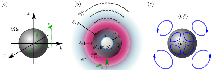
Figure 1: (a) The spherical particle with radius $a$, and the referenced coordinate systems used in the calculation. (b) The incident pressure wave, described by the potential $\phi_{\mathrm{1c}}^{\mathrm{in}}$ and the corresponding scattered response, described by $\phi_{\mathrm{1c}}^{\mathrm{sc}}$, $\phi_{\mathrm{1t}}^{\mathrm{sc}}$, $\bm{\psi}^{\mathrm{sc}}_{1}$, $\phi_{\mathrm{1c}}^{\prime}$, $\phi_{\mathrm{1t}}^{\prime}$, and $\bm{\psi}^{\mathrm{\prime}}_{1}$. (c) the second order time-averaged streaming rolls generated by the first-order wave scattering.

III The first-order problem

We consider a spherical particle with radius $a$ centered in a spherical coordinate system $(r,\theta,\varphi)$ as shown in Fig. 1(a). For a solid particle, we must solve Eq. (26) for $r<a$ and Eq. (15) for $r>a$, whereas for a fluid particle, we must solve Eq. (15) in both regions. Clearly, these two systems of equations have the same structure, and following Karlsen [10], they can be treated in the same manner using unified potential theory.

III.1 Unified potential theory for fluids and solids

To determine $\bm{\psi}_{1}$ in either a solid or a fluid, we must solve Eqs. (15c) and (26c), which both can be written as

$$\nabla^{2}\bm{\psi}_{1}+k_{\mathrm{s}}^{2}\bm{\psi}_{1}=\bm{0},\qquad\text{(fluids and solids)}.$$ (27)

By defining the kinematic viscosity $\nu_{0}$ of a solid as,

$$\nu_{0}=\mathrm{i}\>\frac{c_{\mathrm{tr0}}^{2}}{\omega},\qquad\text{(solids)},$$ (28)

the square of the shear wave number $k_{\mathrm{s}}$ in both fluids and solids can be written as,

$$k_{\mathrm{s}}^{2}=\mathrm{i}\>\frac{\omega}{\nu_{0}},\qquad\text{(fluids and solids)}.$$ (29)

To determine $\phi_{1}$ and $T_{1}$ we solve Eqs. (15a) and (15b) for fluids and Eqs. (26a) and (26b) for solids. In both cases, combining the pair of equations, a single equation for $\phi_{1}$ is obtained,

$$\alpha_{\mathrm{xl}}\nabla^{2}\nabla^{2}\phi_{1}+\beta_{\mathrm{xl}}k_{0}^{2}\nabla^{2}\phi_{1}+k_{0}^{4}\phi_{1}=0,\quad k_{0}=\frac{\omega}{c_{0}}.$$ (30)

Here, $\alpha_{\mathrm{xl}}$ and $\beta_{\mathrm{xl}}$ for fluids ($\mathrm{xl}=\mathrm{fl}$) and solids ($\mathrm{xl}=\mathrm{sl}$) are given by

$$\alpha_{\mathrm{fl}} =-\mathrm{i}(1-\mathrm{i}\gamma_{0}\Gamma_{\mathrm{s}})\Gamma_{\mathrm{t}},\quad \beta_{\mathrm{fl}} =1-\mathrm{i}(\Gamma_{\mathrm{s}}+\gamma_{0}\Gamma_{\mathrm{t}}),$$ (31a)

$$\alpha_{\mathrm{sl}} =-\mathrm{i}(1+X)\Gamma_{\mathrm{t}},\quad \beta_{\mathrm{sl}} =1-\mathrm{i}\gamma_{0}\Gamma_{\mathrm{t}},$$ (31b)

$$\Gamma_{\mathrm{s}} =\frac{(\eta^{\mathrm{b}}_{0}+\frac{4}{3}\eta_{0})\omega}{\rho_{0}c_{0}^{2}}, \Gamma_{\mathrm{t}} =\frac{D^{\mathrm{th}}_{0}\omega}{c_{0}^{2}},$$ (31c)

$$X =(\gamma_{0}-1)(1-\chi), \chi =\frac{1}{\rho_{0}\kappa_{s0}c_{0}^{2}},$$ (31d)

where we have introduced the viscous and thermal damping factors, $\Gamma_{\mathrm{s}}$ and $\Gamma_{\mathrm{t}}$, and the two parameters $X$ and $\chi$. The biharmonic equation (30) is solved by factorization,

$$(\nabla^{2}+k_{\mathrm{c}}^{2})(\nabla^{2}+k_{\mathrm{t}}^{2})\phi_{1}=0,$$ (32)

which combined with (30) yields $k_{\mathrm{c}}^{2}+k_{\mathrm{t}}^{2}=\beta_{\mathrm{xl}}k_{0}^{2}/\alpha_{\mathrm{xl}}$ and $k_{\mathrm{c}}^{2}k_{\mathrm{t}}^{2}=k_{0}^{4}/\alpha_{\mathrm{xl}}$, and thus

$$k_{\mathrm{c}}^{2} =k_{0}^{2}\frac{1}{2\alpha_{\mathrm{xl}}}\bigg{(}\beta_{\mathrm{xl}}-\sqrt{\beta_{\mathrm{xl}}^{2}-4\alpha_{\mathrm{xl}}}\bigg{)},$$ (33a)

$$k_{\mathrm{t}}^{2} =k_{0}^{2}\frac{1}{2\alpha_{\mathrm{xl}}}\bigg{(}\beta_{\mathrm{xl}}+\sqrt{\beta_{\mathrm{xl}}^{2}-4\alpha_{\mathrm{xl}}}\bigg{)}.$$ (33b)

The solution for $\phi_{1}$ is then split into two components

$$\phi_{1}=\phi_{\mathrm{1c}}+\phi_{\mathrm{1t}},$$ (34)

where

$$\nabla^{2}\phi_{\mathrm{1c}}+k_{\mathrm{c}}^{2}\phi_{\mathrm{1c}} =0,$$ (35a)

$$\nabla^{2}\phi_{\mathrm{1t}}+k_{\mathrm{t}}^{2}\phi_{\mathrm{1t}} =0.$$ (35b)

After solving for $\phi_{1}$, $T_{1}$ can be determined in fluids and solids from Eqs. (15a) and (26a),

$$T_{1} =\frac{\mathrm{i}\omega\rho_{0}\kappa_{T0}}{{\alpha_{p0}}}\bigg{[}\phi_{1}+\frac{c_{0}^{2}}{\omega^{2}}\frac{1-\mathrm{i}\gamma_{0}\Gamma_{\mathrm{s}}}{\gamma_{0}}\nabla^{2}\phi_{1}\bigg{]}\text{ (fluids)},$$ (36a)

$$T_{1} =\frac{\mathrm{i}\omega\rho_{0}\kappa_{T0}}{{\alpha_{p0}}}\bigg{[}\phi_{1}+\frac{c_{\mathrm{lo0}}^{2}}{\omega^{2}}\nabla^{2}\phi_{1}\bigg{]}\text{\hskip 36.98857pt (solids)}.$$ (36b)

For the systems we are considering here, $\Gamma_{\mathrm{s}},\Gamma_{\mathrm{t}}\ll 1$, and expanding to first order in these parameters, we find the following wave numbers when using $k_{0}=\omega/c_{0}$,

$$k_{\mathrm{c}} =k_{0}\>\Big{[}1+\frac{\mathrm{i}}{2}[\Gamma_{\mathrm{s}}+(\gamma_{0}-1)\Gamma_{\mathrm{t}}]\Big{]},$$ (37a)

$$k_{\mathrm{t}} =\frac{1+\mathrm{i}}{\delta_{t}}\Big{[}1+\frac{\mathrm{i}}{2}(\gamma_{0}-1)(\Gamma_{\mathrm{s}}-\Gamma_{\mathrm{t}})\Big{]},$$ (37b)

$$k_{\mathrm{s}} =\frac{1+\mathrm{i}}{\delta_{s}},\quad\text{\text@underline{for fluids}},$$ (37c)

and

$$k_{\mathrm{c}} =k_{0}\>\Big{[}1+\frac{\mathrm{i}}{2}(\gamma_{0}-1)\chi\Gamma_{\mathrm{t}}\Big{]},$$ (38a)

$$k_{\mathrm{t}} =\frac{1+\mathrm{i}}{\delta_{t}}\frac{1}{\sqrt{1+X}}\Big{[}1-\frac{\mathrm{i}}{2}(\gamma_{0}-1)\chi\Gamma_{\mathrm{t}}\Big{]},$$ (38b)

$$k_{\mathrm{s}} =\frac{\omega}{c_{\mathrm{tr0}}},\quad\text{\text@underline{for solids}}.$$ (38c)

Here, we have introduced the thermal and viscous boundary layer thicknesses $\delta_{t}$ and $\delta_{s}$ as,

$$\delta_{t}=\sqrt{\frac{2D^{\mathrm{th}}_{0}}{\omega}},\qquad\delta_{s}=\sqrt{\frac{2\nu_{0}}{\omega}}.$$ (39)

To lowest order in $\Gamma_{\mathrm{s}}$ and $\Gamma_{\mathrm{t}}$, we also find that

$$T_{1} =b_{\mathrm{c}}\phi_{\mathrm{1c}}+b_{\mathrm{t}}\phi_{\mathrm{1t}},\;\text{ (fluids and solids)},$$ (40a)

$$b_{\mathrm{c}} =\frac{\mathrm{i}\omega(\gamma_{0}-1)}{{\alpha_{p0}}c_{0}^{2}},\quad b_{\mathrm{t}}=\frac{1}{\chi{\alpha_{p0}}D^{\mathrm{th}}_{0}},$$ (40b)

where $\chi=1$ for fluids. Thus, the governing first-order equations are the same for fluids and solids, only differing by the form of their wave numbers. In fluids, both $k_{\mathrm{t}}$ and $k_{\mathrm{s}}$ describe strongly damped waves, whereas in solids $k_{\mathrm{s}}$ describes a propagating transverse wave.

III.2 Partial-wave expansions and scattering coefficients

Following Karlsen [10], quantities inside the particle ($r<a$) are denoted with a prime, whereas outside in the surrounding fluid medium ($r>a$) they remain unprimed, see Fig. 1(b) and (c). Moreover, a tilde denotes the ratio of a parameter $q^{\prime}_{0}$ inside a particle and $q_{0}$ in the surrounding fluid (in contrast to Doinikov, who uses the tilde to denote particle parameters [4, 5, 6, 7, 8]),

$$\tilde{q}_{0}=\frac{q^{\prime}_{0}}{q_{0}}.$$ (41)

To determine the field solutions of the first-order problem, we consider an axisymmetric incident wave in the surrounding fluid medium, which is far enough away from solid boundaries, such that thermal and viscous modes from there are vanishingly small. When the incident field interacts with the particle, scattered fields are generated. Thus, we write $\phi_{\mathrm{1c}}$ outside the particle as the sum of an incident field and a scattered field, while the remaining potentials only contain a scattered part,

$$\phi_{\mathrm{1c}} =\left\{\begin{array}[]{ll}\phi_{\mathrm{1c}}^{\mathrm{in}}+\phi_{\mathrm{1c}}^{\mathrm{sc}},&r>a,\\ \phi_{\mathrm{1c}}^{\prime},&r<a,\end{array}\right.$$ (42c)

$$\phi_{\mathrm{1t}} =\left\{\begin{array}[]{ll}\phi_{\mathrm{1t}}^{\mathrm{sc}},&r>a,\\ \phi_{\mathrm{1t}}^{\prime},&r<a,\end{array}\right.$$ (42f)

$$\bm{\psi}_{1} =\left\{\begin{array}[]{ll}\bm{\psi}^{\mathrm{sc}}_{1},&r>a,\\ \bm{\psi}^{\mathrm{\prime}}_{1},&r<a.\end{array}\right.$$ (42i)

All potentials $\phi_{\mathrm{1c}}^{\mathrm{in}}$, $\phi_{\mathrm{1c}}^{\mathrm{sc}}$, $\phi_{\mathrm{1t}}^{\mathrm{sc}}$, $\bm{\psi}^{\mathrm{sc}}_{1}$, $\phi_{\mathrm{1c}}^{\prime}$, $\phi_{\mathrm{1t}}^{\prime}$, and $\bm{\psi}^{\mathrm{\prime}}_{1}$ are solutions to Helmholtz equations. Inside the particle for $r<a$, the solutions are written in terms spherical Bessel functions $j_{n}(k^{\prime}_{i}r)$ and Legendre polynomials $P_{n}(\cos\theta)$ to avoid singularities at $r=0$. Outside the particle for $r>a$, the scattered fields are written in terms of the decaying outgoing spherical Hankel functions $h_{n}(k_{i}r)$.
In the surrounding fluid (unprimed), $r>a$

$$\phi_{\mathrm{1c}}^{\mathrm{in}} =\sum_{n=0}^{\infty}\phi_{\mathrm{1c},n}^{\mathrm{in}}(r)P_{n}(\cos\theta),$$ (43a)

$$\text{\; with }\;\phi_{\mathrm{1c},n}^{\mathrm{in}}(r)=A_{n}j_{n}(k_{\mathrm{c}}r),$$

$$\phi_{\mathrm{1c}}^{\mathrm{sc}} =\sum_{n=0}^{\infty}\phi_{\mathrm{1c},n}^{\mathrm{sc}}(r)P_{n}(\cos\theta),$$ (43b)

$$\text{\; with }\;\phi_{\mathrm{1c},n}^{\mathrm{sc}}(r)=A_{n}\alpha_{\mathrm{c},n}^{\mathrm{sc}}h_{n}(k_{\mathrm{c}}r),$$

$$\phi_{\mathrm{1t}}^{\mathrm{sc}} =\sum_{n=0}^{\infty}\phi_{\mathrm{1t},n}^{\mathrm{sc}}(r)P_{n}(\cos\theta),$$ (43c)

$$\text{\; with }\;\phi_{\mathrm{1t},n}^{\mathrm{sc}}(r)=A_{n}\alpha_{\mathrm{t},n}^{\mathrm{sc}}h_{n}(k_{\mathrm{t}}r),$$

$$\bm{\psi}^{\mathrm{sc}}_{1} =\bm{e}_{\varphi}\sum_{n=1}^{\infty}\psi_{1,n}^{\mathrm{sc}}(r)\partial_{\theta}P_{n}(\cos\theta),$$ (43d)

$$\text{\; with }\;\psi_{1,n}^{\mathrm{sc}}(r)=A_{n}\alpha_{\mathrm{s},n}^{\mathrm{sc}}h_{n}(k_{\mathrm{s}}r).$$

Inside the particle (primed), $r<a$

$$\phi_{\mathrm{1c}}^{\prime} =\sum_{n=0}^{\infty}\phi_{\mathrm{1c},n}^{\prime}(r)P_{n}(\cos\theta),$$ (44a)

$$\text{\; with }\;\phi_{\mathrm{1c},n}^{\prime}(r)=A_{n}\alpha_{\mathrm{c},n}^{\prime}j_{n}(k_{\mathrm{c}}^{\prime}r),$$

$$\phi_{\mathrm{1t}}^{\prime} =\sum_{n=0}^{\infty}\phi_{\mathrm{1t},n}^{\prime}(r)P_{n}(\cos\theta),$$ (44b)

$$\text{\; with }\;\phi_{\mathrm{1t},n}^{\prime}(r)=A_{n}\alpha_{\mathrm{t},n}^{\prime}j_{n}(k_{\mathrm{t}}^{\prime}r),$$

$$\bm{\psi}^{\mathrm{\prime}}_{1} =\bm{e}_{\varphi}\sum_{n=1}^{\infty}\psi_{1,n}^{\prime}(r)\partial_{\theta}P_{n}(\cos\theta),$$ (44c)

$$\text{\; with }\;\psi_{1,n}^{\prime}(r)=A_{n}\alpha_{\mathrm{s},n}^{\prime}j_{n}(k_{\mathrm{s}}^{\prime}r).$$

Here, the wave coefficients $A_{n}$ defines the incident wave, and the scattering coefficients $\alpha_{\mathrm{c},n}^{\mathrm{sc}}$, $\alpha_{\mathrm{t},n}^{\mathrm{sc}}$, $\alpha_{\mathrm{s},n}^{\mathrm{sc}}$, $\alpha_{\mathrm{c},n}^{\prime}$, $\alpha_{\mathrm{t},n}^{\prime}$, and $\alpha_{\mathrm{s},n}^{\prime}$ are determined from the boundary conditions (continuous stress, velocity, temperature, and heat flux) at the particle-fluid interface $r=a$. A compact notation $\alpha_{i,n}$, with index $i=0,1,2,3,4,5,6=0,c,t,s,c^{\prime},t^{\prime},s^{\prime}$ and mode number $n=0,1,\ldots$, is introduced for the six scattering coefficients, and when we include unity for the incoming wave for each mode $n$, we obtain

$$\big{\{}\alpha_{i,n}\}_{i=0,1,\ldots,6}=\big{\{}1,\alpha_{\mathrm{c},n}^{\mathrm{sc}},\alpha_{\mathrm{t},n}^{\mathrm{sc}},\alpha_{\mathrm{s},n}^{\mathrm{sc}},\alpha_{\mathrm{c},n}^{\prime},\alpha_{\mathrm{t},n}^{\prime},\alpha_{\mathrm{s},n}^{\prime}\big{\}},$$

$$\quad\text{with }\;i=0,1,2,3,4,5,6=0,c,t,s,c^{\prime},t^{\prime},s^{\prime}.$$ (45)

When imposing the boundary conditions at the particle surface, it is convenient to express the first-order pressure in terms of the potentials,

$$p_{1}=\mathrm{i}\omega\rho_{0}(\phi_{\mathrm{1c}}+\phi_{\mathrm{1t}})-(\eta^{\mathrm{b}}_{0}+\tfrac{4}{3}\eta_{0})(k_{\mathrm{c}}^{2}\phi_{\mathrm{1c}}+k_{\mathrm{t}}^{2}\phi_{\mathrm{1t}}).$$ (46)

The velocity in a solid is given by $\bm{v}_{1}=-\mathrm{i}\omega\bm{u}_{1}$, and using the definition (28) of solid viscosity, we express the first-order stress $\bm{\sigma}_{1}$ for both fluids and solids as,

$$\bm{\sigma}_{1} =\eta_{0}[(2k_{\mathrm{c}}^{2}-k_{\mathrm{s}}^{2})\phi_{\mathrm{1c}}+(2k_{\mathrm{t}}^{2}-k_{\mathrm{s}}^{2})\phi_{\mathrm{1t}}]\,\textbf{{I}}$$

$$\quad+\eta_{0}\Big{[}\bm{\nabla}\bm{v}_{1}+(\bm{\nabla}\bm{v}_{1})^{\textsf{T}}\Big{]},\;\;\text{(fluids and solids)}.$$ (47)

Lastly, from Eqs. (43) and (44) and the definition $\bm{v}_{1}=\bm{\nabla}\phi_{\mathrm{1c}}+\bm{\nabla}\phi_{\mathrm{1t}}+\bm{\nabla}\times\bm{\psi}^{\mathrm{sc}}_{1}$ for both the unprimed and primed first-order velocity, we have the following expressions:

$$v_{1r} =\sum_{n=0}^{\infty}v_{1r}^{n}(r)P_{n}(\cos\theta),$$ (48a)

$$\text{with }\;v_{1r}^{n}(r)=A_{n}\frac{1}{a}\bigg{[}x_{\mathrm{c}}j^{\prime}_{n}(k_{\mathrm{c}}r)+\alpha_{\mathrm{c},n}^{\mathrm{sc}}x_{\mathrm{c}}h^{\prime}_{n}(k_{\mathrm{c}}r)$$

$$\qquad+\alpha_{\mathrm{t},n}^{\mathrm{sc}}x_{\mathrm{t}}h^{\prime}_{n}(k_{\mathrm{t}}r)-\alpha_{\mathrm{s},n}^{\mathrm{sc}}a\frac{n(n+1)}{r}h_{n}(k_{\mathrm{s}}r)\bigg{]},$$

$$v_{1\theta} =\sum_{n=1}^{\infty}v_{1\theta}^{n}(r)\partial_{\theta}P_{n}(\cos\theta),$$ (48b)

$$\text{with }\;v_{1\theta}^{n}(r)=A_{n}\frac{1}{a}\bigg{[}\frac{a}{r}j_{n}(k_{\mathrm{c}}r)+\alpha_{\mathrm{c},n}^{\mathrm{sc}}\frac{a}{r}h_{n}(k_{\mathrm{c}}r)$$

$$\qquad+\alpha_{\mathrm{t},n}^{\mathrm{sc}}\frac{a}{r}h_{n}(k_{\mathrm{t}}r)-\alpha_{\mathrm{s},n}^{\mathrm{sc}}\Big{(}x_{\mathrm{s}}h_{n}^{\prime}(k_{\mathrm{s}}r)+\frac{a}{r}h_{n}(k_{\mathrm{s}}r)\Big{)}\bigg{]},$$

$$v_{1r}^{\prime} =\sum_{n=0}^{\infty}v_{1r}^{n\prime}(r)P_{n}(\cos\theta),$$ (48c)

$$\text{with }\;v_{1r}^{n\prime}(r)=A_{n}\frac{1}{a}\bigg{[}\alpha_{\mathrm{c},n}^{\prime}x_{\mathrm{c}}^{\prime}j^{\prime}_{n}(k_{\mathrm{c}}^{\prime}r)$$

$$\qquad+\alpha_{\mathrm{t},n}^{\prime}x_{\mathrm{t}}^{\prime}j^{\prime}_{n}(k_{\mathrm{t}}^{\prime}r)-\alpha_{\mathrm{s},n}^{\prime}a\frac{n(n+1)}{r}j_{n}(k_{\mathrm{s}}^{\prime}r)\bigg{]},$$

$$v_{1\theta}^{\prime} =\sum_{n=1}^{\infty}v_{1\theta}^{n\prime}(r)\partial_{\theta}P_{n}(\cos\theta),$$ (48d)

$$\text{with }\;v_{1\theta}^{n\prime}(r)=A_{n}\frac{1}{a}\bigg{[}\alpha_{\mathrm{c},n}^{\prime}\frac{a}{r}j_{n}(k_{\mathrm{c}}^{\prime}r)+\alpha_{\mathrm{t},n}^{\prime}\frac{a}{r}j_{n}(k_{\mathrm{t}}^{\prime}r)$$

$$\qquad-\alpha_{\mathrm{s},n}^{\prime}\Big{(}x_{\mathrm{s}}^{\prime}j_{n}^{\prime}(k_{\mathrm{s}}^{\prime}r)+\frac{a}{r}j_{n}(k_{\mathrm{s}}^{\prime}r)\Big{)}\bigg{]},$$

where primed spherical Bessel and Hankel functions refer to differentiation with respect to the argument, and where we have introduced the normalized wave numbers,

$$x_{\mathrm{c}} =k_{\mathrm{c}}a, \quad x_{\mathrm{t}} =k_{\mathrm{t}}a, \quad x_{\mathrm{s}} =k_{\mathrm{s}}a, \quad\text{for }\;r>a,$$ (49a)

$$x_{\mathrm{c}}^{\prime} =k_{\mathrm{c}}^{\prime}a, \quad x_{\mathrm{t}}^{\prime} =k_{\mathrm{t}}^{\prime}a, \quad x_{\mathrm{s}}^{\prime} =k_{\mathrm{s}}^{\prime}a, \quad\text{for }\;r<a.$$ (49b)

The boundary conditions on the particle surface are continuity of velocity, stress, temperature, and heat flux. For a fluid particle, the Young–Laplace pressure $p_{\mathrm{surf}}$ due to the surface tension $\gamma_{\mathrm{surf}}$ is explicitly added as a discontinuity in the normal-stress boundary condition,

$$v_{1r} =v_{1r}^{\prime}, v_{1\theta} =v_{1\theta}^{\prime},$$ (50a)

$$T_{1} =T_{1}^{\prime}, k^{\mathrm{th}}_{0}\partial_{r}T_{1} =k^{\mathrm{th\prime}}_{0}\partial_{r}T_{1}^{\prime},$$ (50b)

$$\sigma_{1\theta r} =\sigma_{1\theta r}^{\prime}, \sigma_{1rr} =\sigma_{1rr}^{\prime}+p_{\mathrm{surf}},$$ (50c)

$$p_{\mathrm{surf}} =-\frac{\mathrm{i}\gamma_{\mathrm{surf}}}{a^{2}\omega} \big{(}\partial_{\theta}^{2}v_{1r}^{\prime}+\partial_{\theta}v_{1r}^{\prime}\cot\theta+2v_{1r}^{\prime}\big{)}\big{|}_{r=a}.$$ (50d)

Here, Eq. (50d) for $p_{\mathrm{surf}}$ is valid for an axisymetrically perturbed spherical surface [8, 29]. Substituting Eq. (48c) into Eq. (50d), and using $\partial_{\theta}^{2}P_{n}(\cos\theta)+\partial_{\theta}P_{n}(\cos\theta)\cot\theta+2P_{n}(\cos\theta)=-(n-1)(n+2)P_{n}(\cos\theta)$, yields,

$$p_{\mathrm{surf}}=\sum_{n=0}^{\infty}\mathrm{i}\frac{\gamma_{\mathrm{surf}}}{a^{2}\omega}(n-1)(n+2)v_{1r}^{n\prime}(a)P_{n}(\cos\theta).$$ (51)

For each value of $n$, the final expressions of the boundary conditions from (50) are,

$$v_{1r}=v_{1r}^{\prime}$$

$$\;\;\alpha_{\mathrm{c},n}^{\mathrm{sc}}x_{\mathrm{c}}h^{\prime}_{n}(x_{\mathrm{c}})+\alpha_{\mathrm{t},n}^{\mathrm{sc}}x_{\mathrm{t}}h^{\prime}_{n}(x_{\mathrm{t}})-\alpha_{\mathrm{s},n}^{\mathrm{sc}}n(n+1)h_{n}(x_{\mathrm{s}})$$

$$\;\;-\alpha_{\mathrm{c},n}^{\prime}x_{\mathrm{c}}^{\prime}j^{\prime}_{n}(x_{\mathrm{c}}^{\prime})-\alpha_{\mathrm{t},n}^{\prime}x_{\mathrm{t}}^{\prime}j^{\prime}_{n}(x_{\mathrm{t}}^{\prime})+\alpha_{\mathrm{s},n}^{\prime}n(n+1)j_{n}(x_{\mathrm{s}}^{\prime})$$

$$\;\;=-x_{\mathrm{c}}j^{\prime}_{n}(x_{\mathrm{c}}),$$ (52a)

$$v_{1\theta}=v_{1\theta}^{\prime}$$

$$\;\;\alpha_{\mathrm{c},n}^{\mathrm{sc}}h_{n}(x_{\mathrm{c}})+\alpha_{\mathrm{t},n}^{\mathrm{sc}}h_{n}(x_{\mathrm{t}})-\alpha_{\mathrm{s},n}^{\mathrm{sc}}\big{[}x_{\mathrm{s}}h_{n}^{\prime}(x_{\mathrm{s}})+h_{n}(x_{\mathrm{s}})\big{]}$$

$$\;\;-\alpha_{\mathrm{c},n}^{\prime}j_{n}(x_{\mathrm{c}}^{\prime})-\alpha_{\mathrm{t},n}^{\prime}j_{n}(x_{\mathrm{t}}^{\prime})+\alpha_{\mathrm{s},n}^{\prime}\big{[}x_{\mathrm{s}}^{\prime}j_{n}^{\prime}(x_{\mathrm{s}}^{\prime})+j_{n}(x_{\mathrm{s}}^{\prime})\big{]}$$

$$\;\;=-j_{n}(x_{\mathrm{c}}),$$ (52b)

$$T_{1}=T_{1}^{\prime}$$

$$\;\;\alpha_{\mathrm{c},n}^{\mathrm{sc}}b_{\mathrm{c}}h_{n}(x_{\mathrm{c}})+\alpha_{\mathrm{t},n}^{\mathrm{sc}}b_{\mathrm{t}}h_{n}(x_{\mathrm{t}})$$

$$\;\;-\alpha_{\mathrm{c},n}^{\prime}b_{\mathrm{c}}^{\prime}j_{n}(x_{\mathrm{c}}^{\prime})-\alpha_{\mathrm{t},n}^{\prime}b_{\mathrm{t}}^{\prime}j_{n}(x_{\mathrm{t}}^{\prime})=-b_{\mathrm{c}}j_{n}(x_{\mathrm{c}}),$$ (52c)

$$k^{\mathrm{th}}_{0}\partial_{r}T_{1}=k^{\mathrm{th\prime}}_{0}\partial_{r}T_{1}^{\prime}$$

$$\;\;\alpha_{\mathrm{c},n}^{\mathrm{sc}}k^{\mathrm{th}}_{0}b_{\mathrm{c}}x_{\mathrm{c}}h_{n}^{\prime}(x_{\mathrm{c}})+\alpha_{\mathrm{t},n}^{\mathrm{sc}}k^{\mathrm{th}}_{0}b_{\mathrm{t}}x_{\mathrm{t}}h_{n}^{\prime}(x_{\mathrm{t}})$$

$$\;\;-\alpha_{\mathrm{c},n}^{\prime}k^{\mathrm{th\prime}}_{0}b_{\mathrm{c}}^{\prime}x_{\mathrm{c}}^{\prime}j_{n}^{\prime}(x_{\mathrm{c}}^{\prime})-\alpha_{\mathrm{t},n}^{\prime}k^{\mathrm{th\prime}}_{0}b_{\mathrm{t}}^{\prime}x_{\mathrm{t}}^{\prime}j_{n}^{\prime}(x_{\mathrm{t}}^{\prime})$$

$$\;\;=-k^{\mathrm{th}}_{0}b_{\mathrm{c}}x_{\mathrm{c}}j_{n}^{\prime}(x_{\mathrm{c}}),$$ (52d)

$$\sigma_{1\theta r}=\sigma_{1\theta r}^{\prime}$$

$$\;\;\alpha_{\mathrm{c},n}^{\mathrm{sc}}2\eta_{0}\big{[}x_{\mathrm{c}}h_{n}^{\prime}(x_{\mathrm{c}})-h_{n}(x_{\mathrm{c}})\big{]}$$

$$\;\;+\alpha_{\mathrm{t},n}^{\mathrm{sc}}2\eta_{0}\big{[}x_{\mathrm{t}}h_{n}^{\prime}(x_{\mathrm{t}})-h_{n}(x_{\mathrm{t}})\big{]}$$

$$\;\;-\alpha_{\mathrm{s},n}^{\mathrm{sc}}\eta_{0}\big{[}x_{\mathrm{s}}^{2}h_{n}^{\prime\prime}(x_{\mathrm{s}})+(n^{2}+n-2)h_{n}(x_{\mathrm{s}})\big{]}$$

$$\;\;-\alpha_{\mathrm{c},n}^{\prime}2\eta_{0}^{\prime}\big{[}x_{\mathrm{c}}^{\prime}j_{n}^{\prime}(x_{\mathrm{c}}^{\prime})\!-\!j_{n}(x_{\mathrm{c}}^{\prime})\big{]}$$

$$\;\;-\alpha_{\mathrm{t},n}^{\prime}2\eta_{0}^{\prime}\big{[}x_{\mathrm{t}}^{\prime}j_{n}^{\prime}(x_{\mathrm{t}}^{\prime})\!-\!j_{n}(x_{\mathrm{t}}^{\prime})\big{]}$$

$$\;\;+\alpha_{\mathrm{s},n}^{\prime}\eta_{0}^{\prime}\big{[}x_{\mathrm{s}}^{\prime 2}j_{n}^{\prime\prime}(x_{\mathrm{s}}^{\prime})+(n^{2}+n-2)j_{n}(x_{\mathrm{s}}^{\prime})\big{]}$$

$$\;\;=-2\eta_{0}\big{[}x_{\mathrm{c}}j_{n}^{\prime}(x_{\mathrm{c}})-j_{n}(x_{\mathrm{c}})\big{]},$$ (52e)

$$\sigma_{1rr}=\sigma_{1rr}^{\prime}+p_{\mathrm{surf}}$$

$$\;\;\alpha_{\mathrm{c},n}^{\mathrm{sc}}\eta_{0}\big{[}(2x_{\mathrm{c}}^{2}-x_{\mathrm{s}}^{2})h_{n}(x_{\mathrm{c}})+2x_{\mathrm{c}}^{2}h_{n}^{\prime\prime}(x_{\mathrm{c}})\big{]}$$

$$\;\;+\alpha_{\mathrm{t},n}^{\mathrm{sc}}\eta_{0}\big{[}(2x_{\mathrm{t}}^{2}-x_{\mathrm{s}}^{2})h_{n}(x_{\mathrm{t}})+2x_{\mathrm{t}}^{2}h_{n}^{\prime\prime}(x_{\mathrm{t}})\big{]}$$

$$\;\;-\alpha_{\mathrm{s},n}^{\mathrm{sc}}\eta_{0}2n(n+1)\big{[}x_{\mathrm{s}}h_{n}^{\prime}(x_{\mathrm{s}})-h_{n}(x_{\mathrm{s}})\big{]}$$

$$\;\;-\alpha_{\mathrm{c},n}^{\prime}\eta_{0}^{\prime}\big{[}(2x_{\mathrm{c}}^{\prime 2}-x_{\mathrm{s}}^{\prime 2})j_{n}(x_{\mathrm{c}}^{\prime})+2x_{\mathrm{c}}^{\prime 2}j_{n}^{\prime\prime}(x_{\mathrm{c}}^{\prime})$$

$$\;\;\qquad\qquad+(n-1)(n+2)\frac{\mathrm{i}\gamma_{\mathrm{surf}}}{a\omega\eta_{0}^{\prime}}x_{\mathrm{c}}^{\prime}j^{\prime}_{n}(x_{\mathrm{c}}^{\prime})\big{]}$$

$$\;\;-\alpha_{\mathrm{t},n}^{\prime}\eta_{0}^{\prime}\big{[}(2x_{\mathrm{t}}^{\prime 2}-x_{\mathrm{s}}^{\prime 2})j_{n}(x_{\mathrm{t}}^{\prime})+2x_{\mathrm{t}}^{\prime 2}j_{n}^{\prime\prime}(x_{\mathrm{t}}^{\prime})$$

$$\;\;\qquad\qquad+(n-1)(n+2)\frac{\mathrm{i}\gamma_{\mathrm{surf}}}{a\omega\eta_{0}^{\prime}}x_{\mathrm{t}}^{\prime}j^{\prime}_{n}(x_{\mathrm{t}}^{\prime})\big{]}$$

$$\;\;+\alpha_{\mathrm{s},n}^{\prime}\eta_{0}^{\prime}\big{[}2n(n+1)(x_{\mathrm{s}}^{\prime}j_{n}^{\prime}(x_{\mathrm{s}}^{\prime})-j_{n}(x_{\mathrm{s}}^{\prime}))$$

$$\;\;\qquad\qquad+(n-1)n(n+1)(n+2)\frac{\mathrm{i}\gamma_{\mathrm{surf}}}{a\omega\eta_{0}^{\prime}}j_{n}(x_{\mathrm{s}}^{\prime})\big{]}$$

$$\;\;=-\eta_{0}\big{[}(2x_{\mathrm{c}}^{2}-x_{\mathrm{s}}^{2})j_{n}(x_{\mathrm{c}})+2x_{\mathrm{c}}^{2}j_{n}^{\prime\prime}(x_{\mathrm{c}})\big{]}.$$ (52f)

We notice that the terms with $n=1$, describing translation of the sphere, are unaffected by the surface tension terms, and that for a solid particle, we have $\gamma_{\mathrm{surf}}=0$. The expressions (52) show that the scattering coefficients $\big{\{}\alpha_{i,n}\big{\}}$, $i=1,2,\ldots,6$, for each mode $n$ can be found by solving the following 6-by-6 matrix equation,

$$\sum_{i=1}^{6}M_{ki,n}\alpha_{i,n}=N_{k,n},\;k=1,2,\ldots,6,\text{ mode }n,$$ (53a)

where the 36 matrix elements $$(\bm{M}_{n})_{ik} n (\bm{N}_{n})_{k}$$ for a given mode can be read off from Eq. (52), as can the 6 vector components on the right-hand side,

$$\bm{N}_{n}=\begin{bmatrix}-x_{\mathrm{c}}j^{\prime}_{n}(x_{\mathrm{c}})\\ -j_{n}(x_{\mathrm{c}})\\ -b_{\mathrm{c}}j_{n}(x_{\mathrm{c}})\\ -k^{\mathrm{th}}_{0}b_{\mathrm{c}}x_{\mathrm{c}}j_{n}^{\prime}(x_{\mathrm{c}})\\ -2\eta_{0}[x_{\mathrm{c}}j_{n}^{\prime}(x_{\mathrm{c}})-j_{n}(x_{\mathrm{c}})]\\ -\eta_{0}[(2x_{\mathrm{c}}^{2}-x_{\mathrm{s}}^{2})j_{n}(x_{\mathrm{c}})+2x_{\mathrm{c}}^{2}j_{n}^{\prime\prime}(x_{\mathrm{c}})]\end{bmatrix}.$$ (53b)

Note that Eqs. (52) and (52) are void for mode $$n=0 4\times 4 n$$, leading to a matrix system in this case of the monopole coefficients. For a given mode , the scattering coefficients can be found by Cramer’s rule,

$$\alpha_{i,n}=\big{|}\bm{M}_{n}\big{|}^{-1}\>\big{|}\bm{M}_{n}^{(i)}\big{|},\quad i=1,2,\ldots,6,$$ (53c)

where $|\dots|$ indicates the determinant, and $\bm{M}_{n}^{(i)}$ is the matrix $\bm{M}_{n}$ with its $i$’th column replaced by $\bm{N}_{n}$.

We consider the long-wavelength limit, where the incident wavelength $\lambda=c_{0}/f$ is much longer than the particle radius and the boundary layer thicknesses, $\lambda\gg a,\delta_{t},\delta_{t}^{\prime},\delta_{s},\delta_{s}^{\prime}$ for fluids and $\lambda,\delta_{s}^{\prime}\gg a,\delta_{t},\delta_{t}^{\prime},\delta_{s}$ for solids. No restrictions are put on the particle radius relative to the boundary-layer thicknesses. The long-wavelength limit is characterized by the small parameter $x_{0}$, in which we develop leading order expressions,

$$x_{0}=k_{0}a=2\pi\frac{a}{\lambda}\ll 1.$$ (54)

It is assumed that all fluids and solids have speeds of sounds—and therefore wavelengths—of roughly the same order of magnitude, leading to

$$|x_{\mathrm{c}}|^{2},|x_{\mathrm{c}}^{\prime}|^{2}\sim x_{0}^{2}.$$ (55)

For the case of either a solid or a fluid particle, the following general scalings hold,

$$\Gamma_{\mathrm{s}},\Gamma_{\mathrm{t}},\frac{|b_{\mathrm{c}}|}{|b_{\mathrm{t}}|},\frac{|b_{\mathrm{c}}^{\prime}|}{|b_{\mathrm{t}}|}\sim x_{0}^{2}.$$ (56)

Lastly, due to the definition of solid viscosity (28) and the difference in solid and fluid shear wave numbers $k_{\mathrm{s}}$, one has the following different scalings for the case of a solid sphere and a fluid sphere, respectively:

$$|x_{\mathrm{s}}^{\prime}|^{2},|\tilde{\eta}_{0}|^{-1}\sim x_{0}^{2}\ll|x_{\mathrm{s}}|^{2},|x_{\mathrm{t}}|^{2},|x_{\mathrm{t}}^{\prime}|^{2}, \text{ (solids)},$$ (57a)

$$x_{0}^{2}\ll|x_{\mathrm{s}}|^{2},|x_{\mathrm{s}}^{\prime}|^{2},|x_{\mathrm{t}}|^{2},|x_{\mathrm{t}}^{\prime}|^{2}, \text{ (fluids)}.$$ (57b)

We expand the determinants in (53c) to lowest order in $x_{0}$, while respecting the scalings in Eqs. (55), (56) and (57), in order to find explicit expressions for the scattering coefficients in the long-wavelength limit. We performed this laborious procedure with the algebraic tool Maple [30]. For a solid, we only need the unprimed scattering coefficients to calculate the radiation force, whereas for a fluid, we also need the primed ones. Only scattering coefficients for $n=0,1,2$ turn out to give significant contributions to the final force expressions. The scattering coefficients for a solid and for a fluid particle are given in Appendices B and C, respectively. We find that the expressions for $\alpha^{\mathrm{sc}}_{\mathrm{c},0}$ and $\alpha^{\mathrm{sc}}_{\mathrm{c},1}$ in solids are identical to those given by Karlsen [10], whereas $\alpha^{\mathrm{sc}}_{\mathrm{c},0}$ for a fluid differ for a non-zero surface tension, $\gamma_{\mathrm{surf}}\neq 0$.

IV The second-order problem

We now turn to the solution of the second-order equations (17) for the pressure $\big{\langle}p_{2}\big{\rangle}$ and streaming $\big{\langle}\bm{v}_{2}\big{\rangle}$. We largely follow the method used by Doinikov [5, 4].

IV.1 The general solution

Firstly, we split the fields into incident and scattered fields (superscript ”in” and ”sc”, respectively) outside the particle, and inside a fluid particle they are described by the transmitted (superscript ”prime”) fields,

$$\big{\langle}\bm{v}_{2}\big{\rangle} =\left\{\begin{array}[]{ll}\big{\langle}\bm{v}_{2}^{\mathrm{in}}\big{\rangle}+\big{\langle}\bm{v}_{2}^{\mathrm{sc}}\big{\rangle},&\quad r>a,\\[5.69054pt] \big{\langle}\bm{v}^{\prime}_{2}\big{\rangle}&\quad r<a,\end{array}\right.$$ (58c)

$$\big{\langle}p_{2}\big{\rangle} =\left\{\begin{array}[]{ll}\big{\langle}p_{2}^{\mathrm{in}}\big{\rangle}+\big{\langle}p_{2}^{\mathrm{sc}}\big{\rangle},&\quad r>a,\\[5.69054pt] \big{\langle}p^{\prime}_{2}\big{\rangle}&\quad r<a.\end{array}\right.$$ (58f)

Here, the second-order incident field $\big{\langle}\bm{v}_{2}^{\mathrm{in}}\big{\rangle}$ is calculated from the governing equations (17) using the given first-order potential $\phi^{\mathrm{in}}_{1c}$ in Eq. (43a) describing the incident first-order wave. Solutions for $\big{\langle}\bm{v}_{2}^{\mathrm{in}}\big{\rangle}$ in the case of standing plane waves, traveling plane waves, and diverging spherical waves are given by Doinikov in Refs. [4, 31]. Below, we show how to solve for the scattered fields ”sc” outside the particle, and note without showing it that the transmitted fields ”prime” inside the particle are solved identically. We do, however, write explicitly when differences in the two solutions occur.

Secondly, we express $\big{\langle}\bm{v}_{2}^{\mathrm{sc}}\big{\rangle}$ and the right-hand side of the Navier–Stokes equation (17b) by Helmholtz decompositions,

$$\big{\langle}\bm{v}_{2}^{\mathrm{sc}}\big{\rangle}=\bm{\nabla}\phi_{2}^{\mathrm{sc}}+\bm{\nabla}\times\bm{\psi}_{2}^{\mathrm{sc}},$$ (59a)

$$-\bm{\nabla}\cdot\big{\langle}\nu_{1}\Big{[}\bm{\nabla}\bm{v}_{1}+(\bm{\nabla}\bm{v}_{1})^{\textsf{T}}\Big{]}+[\nu_{1}^{\mathrm{b}}-\tfrac{2}{3}\nu_{1}](\bm{\nabla}\cdot\bm{v}_{1})\textbf{{I}}\big{\rangle}_{\mathrm{nii}}$$

$$\qquad+\bm{\nabla}\cdot\big{\langle}(\bm{v}_{1}\bm{v}_{1})\big{\rangle}_{\mathrm{nii}}=\nu_{0}\big{(}\bm{\nabla}Q+\bm{\nabla}\times\bm{q}\big{)}.$$ (59b)

The subscript ”nii” (read as ”no-incident-incident”) indicates that all terms containing products of two incident first-order fields are discarded. The source terms $Q$ and $\bm{q}$ are found from the first-order fields $\bm{v}_{1}$, $\nu_{1}$, and $\nu_{1}^{\mathrm{b}}$, and subsequently we determine the potential fields $\phi_{2}^{\mathrm{sc}}$ and $\bm{\psi}_{2}^{\mathrm{sc}}$. We express the terms in Eq. (59) by partial-wave expansions,

$$Q =\frac{1}{a^{2}}\sum_{n=0}^{\infty}Q_{n}({\hat{r}})P_{n}(\cos\theta),$$ (60a)

$$\bm{q} =\bm{e}_{\varphi}\frac{1}{a^{2}}\sum_{n=1}^{\infty}q_{n}({\hat{r}})\partial_{\theta}P_{n}(\theta),$$ (60b)

$$\bm{\nabla}\!\cdot\!\Big{\langle}\bm{v}_{1} \bm{v}_{1}-\!\nu_{1}\Big{[}\bm{\nabla}\bm{v}_{1}\!+\!(\bm{\nabla}\bm{v}_{1})^{\textsf{T}}\Big{]}\!-\!\Big{[}\nu_{1}^{\mathrm{b}}\!-\!\tfrac{2}{3}\nu_{1}\Big{]}(\bm{\nabla}\cdot\bm{v}_{1})\textbf{{I}}\Big{\rangle}_{\mathrm{nii}}$$

$$=\bm{e}_{r}\frac{\nu_{0}}{a^{3}}\sum_{n=0}^{\infty}(2n+1)\chi_{rn}({\hat{r}})P_{n}(\cos\theta)$$

$$\quad-\bm{e}_{\theta}\frac{\nu_{0}}{a^{3}}\sum_{n=1}^{\infty}(2n+1)\chi_{\theta n}({\hat{r}})\partial_{\theta}P_{n}(\cos\theta),$$ (60c)

$$\chi_{rn}({\hat{r}}) =\frac{a^{3}}{2\nu_{0}}\int_{0}^{\pi}\mathrm{d}\theta\>P_{n}(\cos\theta)\sin\theta\>\bm{e}_{r}\cdot\bigg{\{}\bm{\nabla}\cdot$$

$$\Big{\langle}\bm{v}_{1}\bm{v}_{1} \!-\!\nu_{1}\Big{[}\bm{\nabla}\bm{v}_{1}\!+\!(\bm{\nabla}\bm{v}_{1})^{\textsf{T}}\Big{]}\!-\!\Big{[}\nu_{1}^{\mathrm{b}}\!-\!\tfrac{2}{3}\nu_{1}\Big{]}(\bm{\nabla}\cdot\bm{v}_{1})\textbf{{I}}\Big{\rangle}_{\mathrm{nii}}\bigg{\}},$$ (60d)

$$\chi_{\theta n}({\hat{r}})=\frac{-a^{3}}{2n(n+1)\nu_{0}}\int_{0}^{\pi}\!\mathrm{d}\theta\>\big{[}\partial_{\theta}P_{n}(\cos\theta)\big{]}\sin\theta\>\bm{e}_{\theta}\!\cdot\!\bigg{\{}\bm{\nabla}\cdot$$

$$\Big{\langle}\bm{v}_{1}\bm{v}_{1}-\nu_{1}\Big{[}\bm{\nabla}\bm{v}_{1}+(\bm{\nabla}\bm{v}_{1})^{\textsf{T}}\Big{]}-\Big{[}\nu_{1}^{\mathrm{b}}-\tfrac{2}{3}\nu_{1}\Big{]}(\bm{\nabla}\cdot\bm{v}_{1})\textbf{{I}}\Big{\rangle}_{\mathrm{nii}}\bigg{\}},$$ (60e)

where we have introduced the nondimensional radial coordinate ${\hat{r}}=r/a$. Combining Eqs. (59) and (60), we find the following equations for $Q_{n}$ and $q_{n}$:

$${\hat{r}}\partial_{\hat{r}}Q_{n}({\hat{r}})-n(n+1)q_{n}({\hat{r}}) =(2n+1){\hat{r}}\chi_{rn}({\hat{r}}),$$ (61a)

$$-Q_{n}({\hat{r}})+{\hat{r}}\partial_{\hat{r}}q_{n}({\hat{r}})+q_{n}({\hat{r}}) =(2n+1){\hat{r}}\chi_{\theta n}({\hat{r}}).$$ (61b)

By differentiating (61b) and using (61a), we obtain an equation for $q_{n}$,

$$\bigg{[}\partial_{\hat{r}}^{2}+\frac{2}{{\hat{r}}}\partial_{\hat{r}} -\frac{n(n+1)}{{\hat{r}}^{2}}\bigg{]}q_{n}({\hat{r}})$$

$$=\frac{2n+1}{{\hat{r}}}\big{[}\chi_{\theta n}({\hat{r}})+{\hat{r}}\partial_{\hat{r}}\chi_{\theta n}({\hat{r}})+\chi_{rn}({\hat{r}})\big{]}.$$ (62)

The homogeneous solution to this equation is,

$$q_{n}^{\mathrm{hom}}({\hat{r}})=c_{3n}{\hat{r}}^{-(n+1)}+c_{4n}{\hat{r}}^{n}.$$ (63)

A particular solution is found from the Green’s function $G_{n}(\xi,y)$ that solves the inhomogeneous equation,

$$\bigg{[}\partial_{\hat{r}}^{2}+\frac{2}{{\hat{r}}}\partial_{\hat{r}}-\frac{n(n+1)}{{\hat{r}}^{2}}\bigg{]}G_{n}(\xi,{\hat{r}})=\delta({\hat{r}}-\xi).$$ (64)

From standard methods, we determine $G_{n}(\xi,{\hat{r}})$ to be

$$G_{n}(\xi,{\hat{r}})=\begin{cases}-\frac{1}{2n+1}\xi^{-(n-1)}{\hat{r}}^{n},&{\hat{r}}<\xi,\\[5.69054pt] -\frac{1}{2n+1}\xi^{n+2}{\hat{r}}^{-(n+1)},&{\hat{r}}>\xi.\end{cases}$$ (65)

By combining the expressions (63) and (65) for $q_{n}^{\mathrm{hom}}({\hat{r}})$ and $G_{n}(\xi,{\hat{r}})$, we determine $q_{n}({\hat{r}})$, and subsequently, $Q_{n}({\hat{r}})$ is found directly from Eq. (61b). After using integration by parts on the term containing $\partial_{\hat{r}}\chi_{\theta n}({\hat{r}})$, the two solutions become,

$$q_{n}({\hat{r}})=$$

$$-{\hat{r}}^{-(n+1)}\bigg{\{}\!\int_{1}^{\hat{r}}\!\xi^{n+1}\big{[}\chi_{rn}(\xi)-(n+1)\chi_{\theta n}(\xi)\big{]}\,\mathrm{d}\xi-\frac{c_{3n}}{n}\bigg{\}}$$

$$+{\hat{r}}^{n}\bigg{\{}\int_{1}^{\hat{r}}\xi^{-n}[\chi_{rn}(\xi)+n\chi_{\theta n}(\xi)]\,\mathrm{d}\xi-\frac{c_{4n}}{n+1}\bigg{\}},$$ (66a)

$$Q_{n}({\hat{r}})=$$

$${\hat{r}}^{-(n+1)}\bigg{\{}n\int_{1}^{\hat{r}}\xi^{n+1}[\chi_{rn}(\xi)-(n+1)\chi_{\theta n}(\xi)]\,\mathrm{d}\xi-c_{3n}\bigg{\}}$$

$$+{\hat{r}}^{n}\bigg{\{}(n+1)\int_{1}^{\hat{r}}\xi^{-n}[\chi_{rn}(\xi)+n\chi_{\theta n}(\xi)]\,\mathrm{d}\xi-c_{4n}\bigg{\}}.$$ (66b)

Substituting unprimed fields and parameters outside the particle, by primed fields and parameters, the same equations are obeyed inside the particle for $q^{\prime}_{n}$ and $Q^{\prime}_{n}$. The integration constants $c_{3n}$, $c_{4n}$, $c^{\prime}_{3n}$, and $c^{\prime}_{4n}$ are determined later by the boundary conditions at ${\hat{r}}\rightarrow 0$, ${\hat{r}}=1$, and ${\hat{r}}\rightarrow\infty$.

Substituting Eqs. (59a) and (59) into (17) yields

$$\nabla^{2}\phi_{2}^{\mathrm{sc}} =-\frac{1}{\rho_{0}}\bm{\nabla}\cdot\big{\langle}\rho_{1}\bm{v}_{1}\big{\rangle}_{\mathrm{nii}},$$ (67a)

$$\nabla^{2}\bm{\psi}_{2}^{\mathrm{sc}} =\bm{q},$$ (67b)

$$\frac{1}{\rho_{0}}\big{\langle}p_{2}^{\mathrm{sc}}\big{\rangle} =-\nu_{0}Q-(\nu_{0}^{\mathrm{b}}+\tfrac{4}{3}\nu_{0})\>\frac{1}{\rho_{0}}\bm{\nabla}\cdot\big{\langle}\rho_{1}\bm{v}_{1}\big{\rangle}_{\mathrm{nii}}.$$ (67c)

To determine $\phi_{2}^{\mathrm{sc}}$ and $\bm{\psi}_{2}^{\mathrm{sc}}$, we insert the partial-wave expansions

$$\phi_{2}^{\mathrm{sc}} =\sum_{n=0}^{\infty}\phi_{2,n}^{\mathrm{sc}}({\hat{r}})P_{n}(\cos\theta),$$ (68a)

$$\bm{\psi}_{2}^{\mathrm{sc}} =\bm{e}_{\varphi}\sum_{n=1}^{\infty}\psi_{2,n}^{\mathrm{sc}}({\hat{r}})\partial_{\theta}P_{n}(\cos\theta),$$ (68b)

$$\frac{1}{\rho_{0}}\bm{\nabla}\cdot\big{\langle}\rho_{1}\bm{v}_{1}\big{\rangle}_{\mathrm{nii}} =\sum_{n=0}^{\infty}\frac{2n+1}{a^{2}}\mu_{n}({\hat{r}})P_{n}(\cos\theta),$$ (68c)

$$\mu_{n}({\hat{r}}) =\frac{a^{2}}{2\rho_{0}}\int_{0}^{\pi}\bm{\nabla}\cdot\big{\langle}\rho_{1}\bm{v}_{1}\big{\rangle}_{\mathrm{nii}}P_{n}(\cos\theta)\sin\theta\,\mathrm{d}\theta,$$ (68d)

into Eq. (67), and obtain

$$\bigg{[}\partial_{\hat{r}}^{2}+\frac{2}{{\hat{r}}}\partial_{\hat{r}}-\frac{n(n+1)}{{\hat{r}}^{2}}\bigg{]}\phi_{2,n}^{\mathrm{sc}}({\hat{r}}) =-(2n+1)\mu_{n}({\hat{r}}),$$ (69a)

$$\bigg{[}\partial_{\hat{r}}^{2}+\frac{2}{{\hat{r}}}\partial_{\hat{r}}-\frac{n(n+1)}{{\hat{r}}^{2}}\bigg{]}\psi_{2,n}^{\mathrm{sc}}({\hat{r}}) =q_{n}({\hat{r}}).$$ (69b)

The left-hand sides contain the same differential operator as in Eq. (IV.1), so using the same Greens function $G_{n}$ (64) as before, we obtain the solution for $\phi_{2,n}^{\mathrm{sc}}$ and $\psi_{2,n}^{\mathrm{sc}}$,

$$\phi_{2,n}^{\mathrm{sc}}({\hat{r}})={\hat{r}}^{-(n+1)}\bigg{(}\int_{1}^{\hat{r}}\xi^{n+2}\mu_{n}(\xi)\,\mathrm{d}\xi-c_{1n}\bigg{)}$$

$$\hskip 42.67912pt-{\hat{r}}^{n}\bigg{(}\int_{1}^{\hat{r}}\xi^{-(n-1)}\mu_{n}(\xi)\,\mathrm{d}\xi-c_{2n}\bigg{)},$$ (70a)

$$\psi_{2,n}^{\mathrm{sc}}({\hat{r}})=$$

$$-\frac{{\hat{r}}^{-(n+1)}}{2(2n+3)}\bigg{\{}\int_{1}^{\hat{r}}\!\xi^{n+3}[\chi_{rn}(\xi)-(n\!+\!3)\chi_{\theta n}(\xi)]\,\mathrm{d}\xi-c_{6n}\bigg{\}}$$

$$-\frac{{\hat{r}}^{n}}{2(2n-1)}\bigg{\{}\int_{1}^{\hat{r}}\!\xi^{-n+2}[\chi_{rn}(\xi)+(n\!-\!2)\chi_{\theta n}(\xi)]\,\mathrm{d}\xi\!-\!c_{5n}\!\bigg{\}}$$

$$+\frac{{\hat{r}}^{-(n-1)}}{2(2n-1)}\bigg{\{}\int_{1}^{\hat{r}}\xi^{n+1}[\chi_{rn}(\xi)-(n+1)\chi_{\theta n}]\,\mathrm{d}\xi-\frac{c_{3n}}{n}\bigg{\}}$$

$$+\frac{{\hat{r}}^{n+2}}{2(2n+3)}\bigg{\{}\int_{1}^{\hat{r}}\xi^{-n}[\chi_{rn}(\xi)+n\chi_{\theta n}(\xi)]\,\mathrm{d}\xi-\frac{c_{4n}}{n+1}\bigg{\}}.$$ (70b)

The same equations are obeyed by the transmitted potentials $\phi_{2,n}^{\prime}$ and $\psi_{2,n}^{\prime}$ with primed integration constants $c^{\prime}_{in}$. We determine the constants $\big{\{}c^{\prime}_{1n},c^{\prime}_{3n},c^{\prime}_{6n}\big{\}}$ and $\big{\{}c_{2n},c_{4n},c_{5n}\big{\}}$ by insisting that $\big{\langle}\bm{v}^{\prime}_{2}\big{\rangle}$ does not diverge for ${\hat{r}}\rightarrow 0$, and that $\big{\langle}\bm{v}_{2}^{\mathrm{sc}}\big{\rangle}\rightarrow 0$ for ${\hat{r}}\rightarrow\infty$,

$$c_{1n}^{\prime} =-\int_{0}^{1}\xi^{n+2}\mu_{n}^{\prime}(\xi)\,\mathrm{d}\xi,$$ (71a)

$$c_{2n} =\int_{1}^{\infty}\xi^{-(n-1)}\mu_{n}(\xi)\,\mathrm{d}\xi,$$ (71b)

$$c_{3n}^{\prime} =-n\int_{0}^{1}\xi^{n+1}[\chi^{\prime}_{rn}(\xi)-(n+1)\chi^{\prime}_{\theta n}(\xi)]\,\mathrm{d}\xi,$$ (71c)

$$c_{4n} =(n+1)\int_{1}^{\infty}\xi^{-n}[\chi_{rn}(\xi)+n\chi_{\theta n}(\xi)]\,\mathrm{d}\xi,$$ (71d)

$$c_{5n} =\int_{1}^{\infty}\xi^{-(n-2)}[\chi_{rn}(\xi)+(n-2)\chi_{\theta n}(\xi)]\,\mathrm{d}\xi,$$ (71e)

$$c_{6n}^{\prime} =-\int_{0}^{1}\xi^{n+3}[\chi^{\prime}_{rn}(\xi)-(n+3)\chi^{\prime}_{\theta n}(\xi)]\,\mathrm{d}\xi,$$ (71f)

$$c_{5n}^{\prime} =c_{6n}=0.$$ (71g)

The two constants $c^{\prime}_{5n}$ and $c_{6n}$ are set to zero because $c_{5n}^{\prime}$ leads to the same kind of terms in $\big{\langle}\bm{v}_{2}^{\prime}\big{\rangle}$ as those containing $c_{2n}^{\prime}$, and similarly for $c_{6n}$ with respect to $c_{1n}$ in $\big{\langle}\bm{v}_{2}^{\mathrm{sc}}\big{\rangle}$. The remaining four coefficients $c_{1n}$, $c^{\prime}_{2n}$, $c_{3n}$, and $c^{\prime}_{4n}$ are discussed in Sections IV.2 and IV.3 when applying the second-order boundary conditions at ${\hat{r}}=1$.

IV.2 Fluid-solid boundary conditions

For the case of a solid particle, we have no second-order time-averaged motion inside the sphere. Therefore, we only need to determine the two last unprimed constants $c_{1n}$ and $c_{3n}$. This is done through the no-slip boundary condition to second order at ${\hat{r}}=1$, including the Stokes-drift terms [32],

$$\big{\langle}\bm{v}_{2}^{\mathrm{sc}}\big{\rangle}=-\big{\langle}\bm{v}_{2}^{\mathrm{in}}\big{\rangle}-\big{\langle}(\bm{s}_{1}\cdot\bm{\nabla})\bm{v}_{1}\big{\rangle},\quad\bm{s}_{1}=\frac{\mathrm{i}}{\omega}\bm{v}_{1}.$$ (72)

This boundary condition is different from the one used by Doinikov, who replaced $\big{\langle}(\bm{s}_{1}\cdot\bm{\nabla})\bm{v}_{1}\big{\rangle}$ by $\big{\langle}s_{1r}\partial_{r}\bm{v}_{1}\big{\rangle}$ [5, 4]. While this is equivalent for the case of a rigid sphere, it is generally not true for the case of a compressible sphere. We make another expansion on the right-hand side of Eq. (72), where all terms are evaluated at ${\hat{r}}=1$,

$$\big{\langle}\bm{v}_{2}^{\mathrm{in}} \big{\rangle}+\big{\langle}(\bm{s}_{1}\cdot\bm{\nabla})\bm{v}_{1}\big{\rangle}$$

$$=\bm{e}_{r}\frac{1}{a}\sum_{n=0}^{\infty}(2n+1)a_{n}^{\mathrm{sl}}P_{n}(\cos\theta)$$

$$\quad-\bm{e}_{\theta}\frac{1}{a}\sum_{n=1}^{\infty}(2n+1)b_{n}^{\mathrm{sl}}\partial_{\theta}P_{n}(\cos\theta),$$ (73a)

$$a_{n}^{\mathrm{sl}} =\frac{a}{2}\int_{0}^{\pi}\!\bm{e}_{r}\!\cdot\!\Big{[}\big{\langle}\bm{v}_{2}^{\mathrm{in}}\big{\rangle}+\big{\langle}(\bm{s}_{1}\cdot\bm{\nabla})\bm{v}_{1}\big{\rangle}\Big{]}P_{n}(\cos\theta)\sin\theta\,\mathrm{d}\theta,$$ (73b)

$$b_{n}^{\mathrm{sl}} =-\frac{a}{2n(n+1)}\int_{0}^{\pi}\!\bm{e}_{\theta}\!\cdot\!\Big{[}\big{\langle}\bm{v}_{2}^{\mathrm{in}}\big{\rangle}$$

$$\qquad+\big{\langle}(\bm{s}_{1}\cdot\bm{\nabla})\bm{v}_{1}\big{\rangle}\Big{]}\partial_{\theta}P_{n}(\cos\theta)\sin\theta\,\mathrm{d}\theta.$$ (73c)

Using that

$$\big{\langle}\bm{v}_{2}^{\mathrm{sc}}\big{\rangle}=\bm{e}_{r}\sum_{n=0}^{\infty}\frac{1}{a}\bigg{[}\partial_{\hat{r}}\phi_{2,n}^{\mathrm{sc}}({\hat{r}})-\frac{n(n+1)}{{\hat{r}}}\psi_{2,n}^{\mathrm{sc}}({\hat{r}})\bigg{]}P_{n}(\cos\theta)$$

$$+\bm{e}_{\theta}\sum_{n=1}^{\infty}\frac{1}{a}\bigg{[}\frac{1}{{\hat{r}}}\phi_{2,n}^{\mathrm{sc}}({\hat{r}})\!-\!\frac{1}{{\hat{r}}}\psi_{2,n}^{\mathrm{sc}}({\hat{r}})\!-\!\partial_{\hat{r}}\psi_{2,n}^{\mathrm{sc}}({\hat{r}})\bigg{]}\partial_{\theta}P_{n}(\cos\theta),$$ (74)

and inserting the explicit forms (70) for $\phi_{2,n}^{\mathrm{sc}}$ and $\psi_{2,n}^{\mathrm{sc}}$ at ${\hat{r}}=1$, we find two equations for the remaining constants,

$$n(n+1)\bigg{[}\frac{c_{3n}}{2n(2n-1)}+\frac{c_{4n}}{2(n+1)(2n+3)}-\frac{c_{5n}}{2(2n-1)}\bigg{]}$$

$$\qquad+(n+1)c_{1n}+nc_{2n}=-(2n+1)a_{n}^{\mathrm{sl}},$$ (75a)

$$-c_{1n}+c_{2n}+\frac{(2-n)c_{3n}}{2n(2n-1)}+\frac{(n+3)c_{4n}}{2(n+1)(2n+3)}$$

$$\qquad-\frac{(n+1)c_{5n}}{2(2n-1)}=(2n+1)b_{n}^{\mathrm{sl}}.$$ (75b)

As we show in Section V, only $c_{31}$ is needed to evaluate the acoustic radiation force $\bm{F}^{\mathrm{rad}}$, so we refrain from determining $c_{3n}$ for $n\neq 1$ and $c_{1n}$. From (75), we obtain

$$c_{31}=-\frac{3}{2}a_{1}^{\mathrm{sl}}+3b_{1}^{\mathrm{sl}}-\frac{3}{2}c_{21}-\frac{1}{4}c_{41}+\frac{3}{2}c_{51}.$$ (76)

IV.3 Fluid-fluid boundary conditions

For a fluid particle, the second-order time-averaged equations of motion are solved both inside and outside the particle. For the boundary conditions, we follow the method used in Ref. [33]. In this case, we assume that the tangential motion and the tangential stress over the momentary boundary of the particle are continuous. Meanwhile, the structural integrity of the particle-fluid interface is assumed to be upheld by surface tension, such that no time-averaged flow can happen across the momentary boundary, which has no perpendicular motion to second order. The boundary conditions at ${\hat{r}}=1$ for a fluid particle can then be formulated as,

$$\big{\langle}v_{2r}^{\mathrm{sc}}\big{\rangle}=-\big{\langle}v_{2r}^{\mathrm{in}}\big{\rangle}-\big{\langle}(\bm{s}_{1}\cdot\bm{\nabla})\bm{v}_{1}\big{\rangle}\cdot\bm{e}_{r},$$ (77a)

$$\big{\langle}v_{2r}^{\prime}\big{\rangle}=-\big{\langle}(\bm{s}_{1}\cdot\bm{\nabla})\bm{v}_{1}^{\prime}\big{\rangle}\cdot\bm{e}_{r},$$ (77b)

$$\big{\langle}v_{2\theta}^{\mathrm{sc}}\big{\rangle}-\big{\langle}v_{2\theta}^{\prime}\big{\rangle}=$$

$$\qquad-\big{\langle}v_{2\theta}^{\mathrm{in}}\big{\rangle}-\big{\langle}(\bm{s}_{1}\cdot\bm{\nabla})(\bm{v}_{1}-\bm{v}_{1}^{\prime})\big{\rangle}\cdot\bm{e}_{\theta},$$ (77c)

$$\big{\langle}\sigma_{2\theta r}^{\mathrm{sc}}\big{\rangle}-\big{\langle}\sigma_{2\theta r}^{\prime}\big{\rangle}=$$

$$\qquad-\big{\langle}\sigma_{2\theta r}^{\mathrm{in}}\big{\rangle}-\big{\langle}(\bm{s}_{1}\cdot\bm{\nabla})\big{[}(\bm{\sigma}_{1}-\bm{\sigma}_{1}^{\prime})\cdot\bm{e}_{r}\big{]}\big{\rangle}\cdot\bm{e}_{\theta}.$$ (77d)

The time-averaged stress component $\big{\langle}\sigma_{2\theta r}\big{\rangle}$ for the full wave outside the particle is given by

$$\big{\langle}\sigma_{2\theta r}\big{\rangle} =\frac{\eta_{0}}{a}\bigg{[}\frac{1}{{\hat{r}}}\partial_{\theta}\big{\langle}v_{2r}\big{\rangle}-\frac{1}{{\hat{r}}}\big{\langle}v_{2\theta}\big{\rangle}+\partial_{\hat{r}}\big{\langle}v_{2\theta}\big{\rangle}\bigg{]}$$

$$\quad+\frac{1}{a}\bigg{\langle}\eta_{1}\bigg{[}\frac{1}{{\hat{r}}}\partial_{\theta}v_{1r}-\frac{1}{{\hat{r}}}v_{1\theta}+\partial_{\hat{r}}v_{1\theta}\bigg{]}\bigg{\rangle}.$$ (78)

The same expression is obeyed by the stress component $\big{\langle}\sigma_{2\theta r}^{\prime}\big{\rangle}$ with primed fields for the transmitted wave inside the particle. Similar to Section IV.2, we expand the second-order incident fields and the products of first-order fields into partial-wave expansions and insert into Eqs. (77) and (IV.3) the explicit expressions (IV.2) for the second-order scattered and primed fields. At ${\hat{r}}=1$ we then obtain the following four expansion coefficients,

$$a_{n}^{\mathrm{fl}} =\frac{a}{2}\int_{0}^{\pi}\bm{e}_{r}\!\cdot\!\Big{[}\big{\langle}\bm{v}_{2}^{\mathrm{in}}\big{\rangle}+\big{\langle}(\bm{s}_{1}\cdot\bm{\nabla})\bm{v}_{1}\big{\rangle}\Big{]}P_{n}(\cos\theta)\sin\theta\,\mathrm{d}\theta,$$ (79a)

$$a_{n}^{\mathrm{fl\prime}} =\frac{a}{2}\int_{0}^{\pi}\bm{e}_{r}\!\cdot\!\big{\langle}(\bm{s}_{1}\cdot\bm{\nabla})\bm{v}_{1}^{\prime}\big{\rangle}P_{n}(\cos\theta)\sin\theta\,\mathrm{d}\theta,$$ (79b)

$$b_{n}^{\mathrm{fl}} =\frac{-a}{2n(n+1)}\int_{0}^{\pi}\bm{e}_{\theta}\!\cdot\!\Big{[}\big{\langle}\bm{v}_{2}^{\mathrm{in}}\big{\rangle}+\big{\langle}(\bm{s}_{1}\cdot\bm{\nabla})(\bm{v}_{1}-\bm{v}_{1}^{\prime})\big{\rangle}\Big{]}$$

$$\hskip 85.35826pt\times\partial_{\theta}P_{n}(\cos\theta)\sin\theta\,\mathrm{d}\theta,$$ (79c)

$$d_{n}^{\mathrm{fl}} =\frac{-a}{2n(n+1)\eta_{0}}\int_{0}^{\pi}\bigg{\{}\eta_{0}\Big{[}\partial_{\hat{r}}\big{\langle}v_{2\theta}^{\mathrm{in}}\big{\rangle}+\partial_{\theta}\big{\langle}v_{2r}^{\mathrm{in}}\big{\rangle}-\big{\langle}v_{2\theta}^{\mathrm{in}}\big{\rangle}\Big{]}$$

$$\quad+a\big{\langle}(\bm{s}_{1}\cdot\bm{\nabla})\big{[}(\bm{\sigma}_{1}-\bm{\sigma}_{1}^{\prime})\cdot\bm{e}_{r}\big{]}\big{\rangle}\cdot\bm{e}_{\theta}$$

$$\quad+\big{\langle}\eta_{1}(\partial_{\theta}v_{1r}+\partial_{\hat{r}}v_{1\theta}-v_{1\theta})\big{\rangle}$$

$$\quad-\big{\langle}\eta_{1}^{\prime}(\partial_{\theta}v_{1r}^{\prime}+\partial_{\hat{r}}v_{1\theta}^{\prime}-v_{1\theta}^{\prime})\big{\rangle}\bigg{\}}\;\partial_{\theta}P_{n}(\cos\theta)\sin\theta\,\mathrm{d}\theta.$$ (79d)

The resulting four equation for the determination of the unknown constants $c_{1n}$, $c_{2n}^{\prime}$, $c_{3n}$, and $c_{4n}^{\prime}$, become

$$-(2n+1)a_{n}^{\mathrm{fl}}=(n+1)c_{1n}+nc_{2n}+n(n+1)$$

$$\quad\times\bigg{(}\frac{c_{3n}}{2n(2n-1)}+\frac{c_{4n}}{2(n+1)(2n+3)}-\frac{c_{5n}}{2(2n-1)}\bigg{)},$$ (80a)

$$-(2n+1)a_{n}^{\mathrm{fl\prime}}=(n+1)c_{1n}^{\prime}+nc_{2n}^{\prime}+n(n+1)$$

$$\quad\times\bigg{(}\frac{c_{3n}^{\prime}}{2n(2n-1)}+\frac{c_{4n}^{\prime}}{2(n+1)(2n+3)}-\frac{c_{6n}^{\prime}}{2(2n+3)}\bigg{)},$$ (80b)

$$(2n+1)b_{n}^{\mathrm{fl}}=-(c_{1n}-c_{1n}^{\prime})+(c_{2n}-c_{2n}^{\prime})$$

$$\quad-\frac{(n-2)(c_{3n}-c_{3n}^{\prime})}{2n(2n-1)}+\frac{(n+3)(c_{4n}-c_{4n}^{\prime})}{2(n+1)(2n+3)}$$

$$\quad-\frac{(n+1)c_{5n}}{2(2n-1)}-\frac{nc_{6n}^{\prime}}{2(2n+3)},$$ (80c)

$$(2n+1)d_{n}^{\mathrm{fl}}=2(n\!+\!2)(c_{1n}\!-\!\tilde{\eta}_{0}c_{1n}^{\prime})+2(n\!-\!1)(c_{2n}\!-\!\tilde{\eta}_{0}c_{2n}^{\prime})$$

$$\quad+\frac{n^{2}-1}{n(2n-1)}(c_{3n}-\tilde{\eta}_{0}c_{3n}^{\prime})+\frac{n(n+2)(c_{4n}-\tilde{\eta}_{0}c_{4n}^{\prime})}{(n+1)(2n+3)}$$

$$\quad-\frac{(n^{2}-1)c_{5n}}{2n-1}+\frac{\tilde{\eta}_{0}n(n+2)c_{6}^{\prime}}{2n+3}.$$ (80d)

As for the solid particle in Section IV.2, we only need $c_{31}$ to evaluate the acoustic radiation force on a fluid particle,

$$c_{31} =-\frac{3}{2}a_{1}^{\mathrm{fl}}+3b_{1}^{\mathrm{fl}}-\frac{3}{2}c_{21}-\frac{1}{4}c_{41}+\frac{3}{2}c_{51}$$

$$\quad+\frac{1}{1+\tilde{\eta}_{0}}\bigg{[}\bigg{(}-3a_{1}^{\mathrm{fl\prime}}-5c_{11}^{\prime}-\frac{1}{2}c_{31}^{\prime}+\frac{1}{2}c_{61}^{\prime}\bigg{)}\tilde{\eta}_{0}$$

$$\quad-\frac{3}{2}a_{1}^{\mathrm{fl}}-3b_{1}^{\mathrm{fl}}-d_{1}^{\mathrm{fl}}+\frac{1}{2}c_{21}+\frac{1}{4}c_{41}-\frac{1}{2}c_{51}\bigg{]}.$$ (81)

V The acoustic radiation force

With the axisymmetric solutions of the first-order acoustic fields in Section III and the second-order steady fields in Section IV at hand, we can now evaluate the radiation force $\bm{F}^{\mathrm{rad}}$ from Eq. (4). We note that only terms containing scattered fields contribute to $\bm{F}^{\mathrm{rad}}$, such that

$$\bm{F}^{\mathrm{rad}}=\oint_{\partial\Omega_{0}}\Big{[}\big{\langle}\bm{\sigma}^{\mathrm{sc}}_{2}\big{\rangle}-\rho_{0}\big{\langle}\bm{v}_{1}\bm{v}_{1}\big{\rangle}_{\mathrm{nii}}\Big{]}\cdot\bm{n}\,\mathrm{d}S$$

$$=\rho_{0}\oint_{\partial\Omega_{0}}\mathrm{d}S\>\bigg{\{}\nu_{0}\Big{[}\partial_{r}\big{\langle}v_{2\theta}^{\mathrm{sc}}\big{\rangle}-\frac{1}{r}\big{\langle}v_{2\theta}^{\mathrm{sc}}\big{\rangle}+\frac{1}{r}\partial_{\theta}\big{\langle}v_{2r}^{\mathrm{sc}}\big{\rangle}\Big{]}\>\bm{e}_{\theta}$$

$$\quad+\Big{[}2\nu_{0}\partial_{r}\big{\langle}v_{2r}^{\mathrm{sc}}\big{\rangle}+\big{(}\nu_{0}^{\mathrm{b}}\!-\!\tfrac{2}{3}\nu_{0}\big{)}\bm{\nabla}\cdot\big{\langle}\bm{v}_{2}^{\mathrm{sc}}\big{\rangle}-\frac{1}{\rho_{0}}\big{\langle}p_{2}^{\mathrm{sc}}\big{\rangle}\Big{]}\>\bm{e}_{r}$$

$$\quad-\Big{\langle}\bm{v}_{1}\bm{v}_{1}-\nu_{1}\Big{[}\!\bm{\nabla}\bm{v}_{1}\!+\!(\bm{\nabla}\bm{v}_{1})^{\textsf{T}}\!\Big{]}$$

$$\hskip 56.9055pt-\Big{[}\nu_{1}^{\mathrm{b}}\!-\!\tfrac{2}{3}\nu_{1}\Big{]}(\bm{\nabla}\!\cdot\!\bm{v}_{1})\textbf{{I}}\Big{\rangle}_{\mathrm{nii}}\cdot\>\bm{e}_{r}\bigg{\}}.$$ (82)

Using $\mathrm{d}S=a^{2}\sin\theta\>\mathrm{d}\theta\>\mathrm{d}\varphi$ and writing the spherical unit vectors in terms of their cartesian components, only a contribution along the direction of wave propagation $\bm{e}_{z}$ will remain after integrating over the azimuthal angle $\varphi$. In Eq. (V) the terms containing $\big{\langle}\bm{v}_{2}^{\mathrm{sc}}\big{\rangle}$ and $\big{\langle}p^{\mathrm{sc}}_{2}\big{\rangle}$ can be substantially simplified as follows. We first express $\bm{\nabla}\cdot\big{\langle}\bm{v}_{2}^{\mathrm{sc}}\big{\rangle}=\nabla^{2}\phi_{2}^{\mathrm{sc}}$ and $\big{\langle}p^{\mathrm{sc}}_{2}\big{\rangle}$ by the right-hand sides of Eq. (67a) and Eq. (67c), respectively. Then we insert the expressions (IV.2), (60a) and (68c) for $\big{\langle}\bm{v}_{2}^{\mathrm{sc}}\big{\rangle}$, $Q$, and $\frac{1}{\rho_{0}}\big{\langle}\rho_{1}\bm{v}_{1}\big{\rangle}_{\mathrm{nii}}$, respectively. Using the Legendre orthogonal relations Eq. (111), the $\theta$ integrals are carried out, leaving only partial-wave contributions with $n=1$. A further simplification is obtained by grouping the terms with $\phi^{\mathrm{sc}}_{2,1}$ and $\psi^{\mathrm{sc}}_{2,1}$, respectively, and noting that the left-hand-sides of Eq. (69) appear with ${\hat{r}}=1$, and thus they can be substituted by the much simpler right-hand sides. In the final expression, only $Q_{1}(1)$ and $q_{1}(1)$ appear, with values given by Eq. (66) for $n=1$ and ${\hat{r}}=1$. The resulting simplified expression for $\bm{F}^{\mathrm{rad}}$ Eq. (V) becomes,

$$\bm{F}^{\mathrm{rad}}=-4\pi\rho_{0}\nu_{0}c_{31}\>\bm{e}_{z}-\rho_{0}\oint_{\partial\Omega_{0}}\mathrm{d}S\>\Big{\langle}\bm{v}_{1}\bm{v}_{1}$$

$$-\!\nu_{1}\Big{[}\bm{\nabla}\bm{v}_{1}\!+\!(\bm{\nabla}\bm{v}_{1})^{\textsf{T}}\Big{]}\!-\!\Big{[}\nu_{1}^{\mathrm{b}}\!-\!\tfrac{2}{3}\nu_{1}\Big{]}(\bm{\nabla}\cdot\bm{v}_{1})\textbf{{I}}\Big{\rangle}_{\mathrm{nii}}\!\!\cdot\bm{e}_{r}.$$ (83)

Inspection of the constant $c_{31}$, which is given by Eqs. (76) and (IV.3) for a solid and fluid particle, respectively, reveals two types of contributions: terms containing the steady $\big{\langle}\bm{v}_{2}^{\mathrm{in}}\big{\rangle}$ and terms containing time-averaged products of the first-order acoustic fields. Consequently, it is convenient to split $\bm{F}^{\mathrm{rad}}$ into two contributions: $\bm{F}^{\mathrm{rad}}_{11}$ containing the time-averaged first-order products, and $\bm{F}^{\mathrm{rad}}_{2,\mathrm{in}}$ containing the streaming velocity $\big{\langle}\bm{v}_{2}^{\mathrm{in}}\big{\rangle}$ of the incident wave,

$$\bm{F}^{\mathrm{rad}}=\bm{F}^{\mathrm{rad}}_{11}+\bm{F}^{\mathrm{rad}}_{2,\mathrm{in}}.$$ (84)

The final step in the calculation is the evaluation of $\bm{F}^{\mathrm{rad}}_{11}$ and $\bm{F}^{\mathrm{rad}}_{2,\mathrm{in}}$. This is a particularly tedious part of the calculation that is best treated for solid and fluid particles separately, in the ensuing two subsections.

V.1 Solid particle

For a solid particle, we evaluate expression (V) for $\bm{F}^{\mathrm{rad}}$ by inserting $c_{31}$ from Eq. (76), which can be expressed explicitly in terms of the time-averaged products of first-order acoustic fields known from Section III.2, and terms including the known field $\big{\langle}\bm{v}_{2}^{\mathrm{in}}\big{\rangle}$ discussed after Eq. (58). To do this, we insert the explicit expressions (73b) and (73) for $a_{1}^{\mathrm{sl}}$ and $b_{1}^{\mathrm{sl}}$, as well as the relations (71) for $c_{21}$, $c_{41}$, and $c_{51}$ with $\mu_{1}(\xi)$, $\chi_{r1}(\xi)$, and $\chi_{\theta 1}(\xi)$ from Eqs. (68d), (60) and (60), respectively. We notice that $\big{\langle}\bm{v}_{2}^{\mathrm{in}}\big{\rangle}$ appears only in some terms of $a_{1}^{\mathrm{sl}}$ and $b_{1}^{\mathrm{sl}}$, and these are thus grouped and manipulated to obtain $\bm{F}^{\mathrm{rad}}_{2,\mathrm{in}}$ for a solid particle as,

$$\bm{F}^{\mathrm{rad}}_{2,\mathrm{in}}=\bm{e}_{z}\>\frac{3\eta_{0}}{2a}\oint_{\partial\Omega_{0}}\mathrm{d}S\>\big{\langle}v_{2z}^{\mathrm{in}}\big{\rangle}.$$ (85)

This corresponds to the Stokes drag on the particle generated by the steady streaming of the incident wave.

Next, we compute $\bm{F}^{\mathrm{rad}}_{11}$, which contains the remainder of the terms, all involving time-averaged products of first-order acoustic fields. It is convenient to rewrite the two terms arising from $c_{41}$ and $c_{51}$, Eqs. (71d) and (71e) with $n=1$, as detailed in Appendix D,

$$-\bm{e}_{z}4\pi\rho_{0}\nu_{0}\bigg{(}\frac{3}{2}c_{51}-\frac{1}{4}c_{41}\bigg{)}$$

$$=\rho_{0}\oint_{\partial\Omega_{0}}\mathrm{d}S\>\Big{\langle}\bm{v}_{1}\bm{v}_{1}-\nu_{1}\Big{[}\bm{\nabla}\bm{v}_{1}+(\bm{\nabla}\bm{v}_{1})^{\textsf{T}}\Big{]}-[\nu_{1}^{\mathrm{b}}-\tfrac{2}{3}\nu_{1}](\bm{\nabla}\cdot\bm{v}_{1})\textbf{{I}}\Big{\rangle}_{\mathrm{nii}}\!\cdot\bm{e}_{r}$$

$$\quad-\bm{e}_{z}3\pi\rho_{0}a^{2}\int_{1}^{\infty}\mathrm{d}\xi\int_{0}^{\pi}\mathrm{d}\theta\>\sin\theta\>\big{[}1-\xi^{-2}\big{]}\;\bm{e}_{r}\cdot\Big{\langle}\bm{v}_{1}\bm{v}_{1}-\nu_{1}\Big{[}\bm{\nabla}\bm{v}_{1}+(\bm{\nabla}\bm{v}_{1})^{\textsf{T}}\Big{]}-[\nu_{1}^{\mathrm{b}}-\tfrac{2}{3}\nu_{1}](\bm{\nabla}\cdot\bm{v}_{1})\textbf{{I}}\Big{\rangle}_{\mathrm{nii}}\!\cdot\bm{e}_{z}$$

$$\quad-\bm{e}_{z}3\pi\rho_{0}a^{3}\int_{1}^{\infty}\mathrm{d}\xi\int_{0}^{\pi}\mathrm{d}\theta\>\sin^{2}\theta\frac{1}{2}\big{[}\xi\!-\!\xi^{-1}\big{]}\Big{\{}\bm{\nabla}\cdot\Big{\langle}\bm{v}_{1}\bm{v}_{1}-\nu_{1}\Big{[}\bm{\nabla}\bm{v}_{1}\!+\!(\bm{\nabla}\bm{v}_{1})^{\textsf{T}}\Big{]}-[\nu_{1}^{\mathrm{b}}\!-\!\tfrac{2}{3}\nu_{1}](\bm{\nabla}\cdot\bm{v}_{1})\textbf{{I}}\Big{\rangle}_{\mathrm{nii}}\Big{\}}\cdot\bm{e}_{\theta}.$$ (86)

We note that the term with the surface integral ”$\oint_{\partial\Omega_{0}}$” also appears in Eq. (V), but with opposite sign, and it thus cancels out. After similarly manipulating $a_{1}^{\mathrm{sl}}$, $b_{1}^{\mathrm{sl}}$, and $c_{21}$, $\bm{F}^{\mathrm{rad}}_{11}$ becomes,

$$\bm{F}^{\mathrm{rad}}_{11} =-\bm{e}_{z}3\pi\rho_{0}\bigg{\{}-\frac{a^{2}\nu_{0}}{\rho_{0}}\int_{1}^{\infty}\mathrm{d}\xi\int_{0}^{\pi}\mathrm{d}\theta\>\cos\theta\sin\theta\bm{\nabla}\cdot\frac{1}{2}\operatorname{Re}[\rho_{1}\bm{v}_{1}^{*}]_{\mathrm{nii}}$$ (87)

$$+a^{2}\int_{1}^{\infty}\mathrm{d}\xi\int_{0}^{\pi}\mathrm{d}\theta\>\sin\theta\big{[}1-\xi^{-2}\big{]}\frac{1}{2}\operatorname{Re}\bigg{[}\bm{e}_{r}\cdot\Big{(}\bm{v}_{1}\bm{v}_{1}^{*}-\nu_{1}\Big{[}\bm{\nabla}\bm{v}_{1}+(\bm{\nabla}\bm{v}_{1})^{\textsf{T}}\Big{]}^{*}-\Big{[}\nu_{1}^{\mathrm{b}}-\tfrac{2}{3}\nu_{1}\Big{]}(\bm{\nabla}\cdot\bm{v}_{1}^{*})\textbf{{I}}\Big{)}\cdot\bm{e}_{z}$$

$$\hskip 56.9055pt+\frac{1}{2}a\xi\Big{\{}\bm{\nabla}\cdot\Big{(}\bm{v}_{1}\bm{v}_{1}^{*}-\nu_{1}\Big{[}\bm{\nabla}\bm{v}_{1}+(\bm{\nabla}\bm{v}_{1})^{\textsf{T}}\Big{]}^{*}-\Big{[}\nu_{1}^{\mathrm{b}}-\tfrac{2}{3}\nu_{1}\Big{]}(\bm{\nabla}\cdot\bm{v}_{1}^{*})\textbf{{I}}\Big{)}\Big{\}}\cdot\bm{e}_{\theta}\sin\theta\bigg{]}_{\mathrm{nii}}$$

$$+\int_{0}^{\pi}\!\mathrm{d}\theta\>\frac{\sin\theta}{2}\operatorname{Re}\bigg{[}\frac{a^{3}}{x_{\mathrm{s}}^{2}}\Big{(}v_{1r}\partial_{r}v_{1r}^{*}+\frac{1}{r}v_{1\theta}\partial_{\theta}v_{1r}^{*}-\frac{1}{r}v_{1\theta}v_{1\theta}^{*}\Big{)}\cos\theta-\frac{a^{3}}{x_{\mathrm{s}}^{2}}\Big{(}v_{1r}\partial_{r}v_{1\theta}^{*}+\frac{1}{r}v_{1\theta}\partial_{\theta}v_{1\theta}^{*}-\frac{1}{r}v_{1r}v_{1\theta}^{*}\Big{)}\sin\theta\bigg{]}_{{\hat{r}}=1}\bigg{\}}.$$

At this point, we need explicit relations for $\rho_{1}$, $\nu_{1}$, and $\nu_{1}^{\mathrm{b}}$. Combining Eqs. (11a), (14) and (35) leads to $\rho_{1}$,

$$\rho_{1} =-\frac{\rho_{0}}{\nu_{0}x_{\mathrm{s}}^{2}}\big{(}x_{\mathrm{c}}^{2}\phi_{\mathrm{1c}}+x_{\mathrm{t}}^{2}\phi_{\mathrm{1t}}\big{)}.$$ (88a)

This is used alongside $$T_{1} \eta_{1} \eta^{\mathrm{b}}_{1}$$ from Eq. (40) in the first-order expansions for and (see Eq. (2b)) to reach,

$$\nu_{1} =\frac{x_{\mathrm{c}}^{2}}{x_{\mathrm{s}}^{2}}B_{\mathrm{c}}\phi_{\mathrm{1c}}+\frac{x_{\mathrm{t}}^{2}}{x_{\mathrm{s}}^{2}}B_{\mathrm{t}}\phi_{\mathrm{1t}},$$ (88b)

$$\nu_{1}^{\mathrm{b}} =\frac{x_{\mathrm{c}}^{2}}{x_{\mathrm{s}}^{2}}B_{\mathrm{c}}^{\mathrm{b}}\phi_{\mathrm{1c}}+\frac{x_{\mathrm{t}}^{2}}{x_{\mathrm{s}}^{2}}B_{\mathrm{t}}^{\mathrm{b}}\phi_{\mathrm{1t}}.$$ (88c)

Here, we have introduced $B_{\mathrm{c}}$, $B_{\mathrm{t}}$, $B_{\mathrm{c}}^{\mathrm{b}}$, and $B_{\mathrm{t}}^{\mathrm{b}}$ that to lowest order in $x_{0}$ become,

$$B_{\mathrm{c}} =\bigg{[}\frac{1-\gamma_{0}}{{\alpha_{p0}}\eta_{0}}\bigg{(}\frac{\partial\eta}{\partial T}\bigg{)}_{T_{0}}-\frac{\rho_{0}}{\eta_{0}}\bigg{(}\frac{\partial\eta}{\partial\rho}\bigg{)}_{\rho_{0}}\bigg{]},$$ (89a)

$$B_{\mathrm{t}} =\bigg{[}\frac{1}{{\alpha_{p0}}\eta_{0}}\bigg{(}\frac{\partial\eta}{\partial T}\bigg{)}_{T_{0}}-\frac{\rho_{0}}{\eta_{0}}\bigg{(}\frac{\partial\eta}{\partial\rho}\bigg{)}_{\rho_{0}}\bigg{]},$$ (89b)

$$B_{\mathrm{c}}^{\mathrm{b}} =\bigg{[}\frac{1-\gamma_{0}}{{\alpha_{p0}}\eta_{0}}\bigg{(}\frac{\partial\eta^{\mathrm{b}}}{\partial T}\bigg{)}_{T_{0}}-\frac{\rho_{0}}{\eta_{0}}\bigg{(}\frac{\partial\eta^{\mathrm{b}}}{\partial\rho}\bigg{)}_{\rho_{0}}\bigg{]},$$ (89c)

$$B_{\mathrm{t}}^{\mathrm{b}} =\bigg{[}\frac{1}{{\alpha_{p0}}\eta_{0}}\bigg{(}\frac{\partial\eta^{\mathrm{b}}}{\partial T}\bigg{)}_{T_{0}}-\frac{\rho_{0}}{\eta_{0}}\bigg{(}\frac{\partial\eta^{\mathrm{b}}}{\partial\rho}\bigg{)}_{\rho_{0}}\bigg{]}.$$ (89d)

Now, we insert Eq. (88) into (87) with $\phi_{\mathrm{1c}}$, $\phi_{\mathrm{1t}}$, and $\bm{v}_{1}$ from Eqs. (43) and (48) to reach an explicit relation for $\bm{F}^{\mathrm{rad}}_{11}$ that can be evaluated analytically. The result is a double sum over mode indices $n$ and $m$, where all terms contain quadratic combinations of scattering coefficients $\alpha_{i,n}$, but only the unprimed ones $\big{\{}\alpha_{i,n}\}_{i=0,1,2,3}=\big{\{}1,\alpha_{\mathrm{c},n}^{\mathrm{sc}},\alpha_{\mathrm{t},n}^{\mathrm{sc}},\alpha_{\mathrm{s},n}^{\mathrm{sc}}\big{\}}$. After evaluating the integrals over $\theta$, see Eq. (111), and switching dummy indices (e.g. $[n-1]\rightarrow n$) as well as complex conjugation (e.g. $\operatorname{Re}\big{[}v_{1r}^{n*}v_{1r}^{n+1}\big{]}=\operatorname{Re}\big{[}v_{1r}^{n}v_{1r}^{n+1*}\big{]}$), one obtains a single sum where all terms contain $A_{n}A^{*}_{n+1}\alpha_{i,n}\alpha_{k,n+1}^{*}$, as detailed in the Supplemental Material [24]. The resulting form of $\bm{F}^{\mathrm{rad}}_{11}$ is,

$$\bm{F}^{\mathrm{rad}}_{11} =-\bm{e}_{z}3\pi\rho_{0}\sum_{n=0}^{\infty}\frac{n+1}{(2n+1)(2n+3)}\operatorname{Re}[A_{n}A_{n+1}^{*}D_{n}],$$ (90a)

$$D_{n} =\sum_{i,k=0}^{3}S_{ik,n}\alpha_{i,n}\alpha_{k,n+1}^{*},$$ (90b)

where we have introduced the force coefficient $D_{n}$ and the 16 second-order coefficients $S_{ik,n}$ for $i,k=0,1,2,3$ for each mode $n$. The explicit expressions for $S_{ik,n}$ are determined by grouping all terms with specific quadratic combinations $\alpha_{i,n}\alpha_{k,n+1}^{*}$ of the first-order scattering coefficients $\alpha_{i,n}$. We have made extensive use of the algebraic tool Maple [30] to derive $S_{ik,n}$ analytically, as listed in Section S3 A of the Supplemental Material [24]. This ends the analysis of $\bm{F}^{\mathrm{rad}}$ for a solid particle, and we now proceed to the case of a fluid particle.

V.2 Fluid particle

For a fluid particle, we use the same computational method as for a solid particle. We insert expression (IV.3) for $c_{31}$ into Eq. (V) for $\bm{F}^{\mathrm{rad}}$. We subsequently substitute the explicit expressions (79) for $a_{n}^{\mathrm{fl}}$, $a_{n}^{\mathrm{fl\prime}}$, $b_{n}^{\mathrm{fl}}$ and $d_{n}^{\mathrm{fl}}$, as well as the relations (71) for $c^{\prime}_{11}$, $c_{21}$, $c^{\prime}_{31}$, $c_{41}$, $c_{51}$, and $c^{\prime}_{61}$ with $\mu_{1}(\xi)$, $\chi_{r1}(\xi)$, and $\chi_{\theta 1}(\xi)$ from Eqs. (68d), (60) and (60), respectively, and with $\mu^{\prime}_{1}(\xi)$, $\chi^{\prime}_{r1}(\xi)$, and $\chi^{\prime}_{\theta 1}(\xi)$ also from from Eqs. (68d), (60) and (60) but with all unprimed fields and parameters substituted by primed quantities. Each term is then evaluated separately, and their contributions to the force are summed up. The resulting expression for $\bm{F}^{\mathrm{rad}}_{11}$ for a fluid particle has the same form as for a solid particle, however, now with 49 second-order coefficients $S_{ik,n}$ with $i,k=0,1,2,\ldots,7$ for each mode $n$, because in contrast to a solid particle, the three transmitted scattering coefficients $\alpha_{\mathrm{c},n}^{\prime}$, $\alpha_{\mathrm{t},n}^{\prime}$, and $\alpha_{\mathrm{s},n}^{\prime}$ are also included,

$$\bm{F}^{\mathrm{rad}}_{11} =-3\pi\rho_{0}\sum_{n=0}^{\infty}\frac{n+1}{(2n+1)(2n+3)}\operatorname{Re}[A_{n}A_{n+1}^{*}D_{n}]\>\bm{e}_{z},$$ (91a)

$$D_{n} =\sum_{i,k=0}^{6}S_{ik,n}\alpha_{i,n}\alpha_{k,n+1}^{*}.$$ (91b)

General expressions for the 49 second-order coefficients $S_{ik,n}$ for a fluid are given in Section S3 B of the Supplemental Material [24].

The contribution to $\bm{F}^{\mathrm{rad}}$ from the second-order incident field $\big{\langle}\bm{v}_{2}^{\mathrm{in}}\big{\rangle}$ in Eq. (IV.3), is found in analogy with the solid-particle case Eq. (85),

$$\bm{F}^{\mathrm{rad}}_{2,\mathrm{in}} =\bm{e}_{z}\bigg{\{}\frac{3\eta_{0}}{2a}\oint_{\partial\Omega_{0}}\mathrm{d}S\>\big{\langle}v_{2z}^{\mathrm{in}}\big{\rangle}+\frac{\pi\eta_{0}a}{1+\tilde{\eta}_{0}}\int_{0}^{\pi}\mathrm{d}\theta\>\sin\theta$$

$$\times\bigg{[}3\Big{(}\big{\langle}v_{2r}^{\mathrm{in}}\big{\rangle}\cos\theta+\big{\langle}v_{2\theta}^{\mathrm{in}}\big{\rangle}\sin\theta\Big{)}$$

$$+\Big{(}\partial_{\hat{r}}\big{\langle}v_{2\theta}^{\mathrm{in}}\big{\rangle}+\partial_{\theta}\big{\langle}v_{2r}^{\mathrm{in}}\big{\rangle}-\big{\langle}v_{2\theta}^{\mathrm{in}}\big{\rangle}\Big{)}\sin\theta\bigg{]}_{{\hat{r}}=1}\bigg{\}}.$$ (92)

V.3 F${}^{\textbf{rad}}$ in the long-wavelength limit x${}_{\textbf{0}}$ $\ll$ 1

To leading order in the dimensionless wave number (54) $x_{0}=k_{0}a$, only $D_{0}$ and $D_{1}$ contribute to $\bm{F}^{\mathrm{rad}}_{11}$ for both solid and fluid particles,

$$\bm{F}^{\mathrm{rad}}_{11} =-\pi\rho_{0}\operatorname{Re}\bigg{[}A_{0}A_{1}^{*}D_{0}+\frac{2}{5}A_{1}A_{2}^{*}D_{1}\bigg{]}\bm{e}_{z},$$ (93a)

$$D_{0} =\sum_{i,k=0}^{N}S_{ik,0}\alpha_{i,0}\alpha^{*}_{k,1}\propto x_{0}^{3},$$ (93b)

$$D_{1} =\sum_{i,k=0}^{N}S_{ik,1}\alpha_{i,1}\alpha^{*}_{k,2}\propto x_{0}^{3},$$ (93c)

$$\quad\text{for }\;x_{0}\ll 1\;\text{with}\;N=3\;(6)\text{ for solids (fluids)},$$

where the leading order $x_{0}^{3}$ of $D_{0}$ and $D_{1}$ is shown. The terms contributing to this leading order are given in Appendices B (solids) and C (fluids) for $\alpha_{i,n}$ and in Appendices E (solids) and F (fluids) for $S_{ik,0}$ and $S_{ik,1}$.

The result in Eq. (93) can be expressed in terms of $p_{1}^{\mathrm{in}}$ and $\bm{v}_{1}^{\mathrm{in}}$ and brought to the familiar form used in the literature [3, 9, 10]. In the long-wavelength limit, $\Gamma_{\mathrm{s}}$ and $\Gamma_{\mathrm{t}}$ are negligible compared to unity, so $k_{\mathrm{c}}\approx k_{0}$ in Eq. (37a). From the properties of $j_{n}(k_{\mathrm{c}}r)$ and $P_{n}(\cos\theta)$, we derive the following from Eq. (43a),

$$\phi_{\mathrm{1c}}^{\mathrm{in}}\bm{\nabla}\phi_{\mathrm{1c}}^{\mathrm{in*}}\big{|}_{{\hat{r}}=0} =\frac{1}{3}k_{\mathrm{c0}}A_{0}A_{1}^{*}\>\bm{e}_{z},$$ (94a)

$$(\bm{\nabla}\phi_{\mathrm{1c}}^{\mathrm{in}}\cdot\bm{\nabla})\bm{\nabla}\phi_{\mathrm{1c}}^{\mathrm{in*}}\big{|}_{{\hat{r}}=0} =\bigg{[}\frac{2A_{1}A_{2}^{*}k_{\mathrm{c0}}^{3}}{45}-\frac{A_{1}A_{0}^{*}k_{\mathrm{c0}}^{3}}{9}\bigg{]}\bm{e}_{z}.$$ (94b)

We use $\bm{v}_{1}^{\mathrm{in}}=\bm{\nabla}\phi_{\mathrm{1c}}^{\mathrm{in}}$ and $p_{1}^{\mathrm{in}}\approx\mathrm{i}\omega\rho_{0}\phi_{\mathrm{1c}}^{\mathrm{in}}$ from Eq. (46) and combine Eq. (94) with Eq. (93), to derive

$$\bm{F}^{\mathrm{rad}}_{11} =-\pi a^{3}\bigg{\{}\frac{2\kappa_{s0}}{3}\operatorname{Re}\bigg{[}\frac{9(D_{0}+D_{1}^{*})}{2x_{0}^{3}}p_{1}^{\mathrm{in}}\bm{\nabla}p_{1}^{\mathrm{in*}}\bigg{]}$$

$$\qquad-\rho_{0}\operatorname{Re}\bigg{[}-\frac{9D_{1}}{x_{0}^{3}}(\bm{v}_{1}^{\mathrm{in}}\cdot\bm{\nabla})\bm{v}_{1}^{\mathrm{in*}}\bigg{]}\bigg{\}}_{{\hat{r}}=0}.$$ (95)

$\bm{F}^{\mathrm{rad}}_{11}$ is equal to $\bm{F}^{\mathrm{rad}}$ derived by Settnes and Bruus [9] and by Karlsen and Bruus [10] when substituting their monopole and dipole coefficients $f_{0}$ and $f_{1}$ by,

$$f_{0}\rightarrow\frac{9(D_{0}+D_{1}^{*})}{2x_{0}^{3}},\qquad f_{1}\rightarrow-\frac{9D_{1}}{x_{0}^{3}}.$$ (96)

For a solid particle, the long-wavelength limit of $\bm{F}^{\mathrm{rad}}_{2,\mathrm{in}}$ is found from Eq. (85) by noting that $\big{\langle}v_{2z}^{\mathrm{in}}\big{\rangle}$ does not vary much across the particle surface, thus

$$\bm{F}^{\mathrm{rad}}_{2,\mathrm{in}}\approx 6\pi\eta_{0}a\big{\langle}v_{2z}^{\mathrm{in}}\big{\rangle}\big{|}_{r=0}\>\bm{e}_{z}.$$ (97)

For a fluid particle, the long-wavelength limit of $\bm{F}^{\mathrm{rad}}_{2,\mathrm{in}}$ is found from Eq. (V.2) by first noting that $\big{|}\partial_{\hat{r}}\big{\langle}v_{2\theta}^{\mathrm{in}}\big{\rangle}\big{|}\sim\big{|}\frac{a}{\lambda}\big{\langle}v_{2\theta}^{\mathrm{in}}\big{\rangle}\big{|}$, which is neglected compared to the remaining terms in Eq. (V.2), and then by making the approximation

$$\big{\langle}\bm{v}_{2}^{\mathrm{in}}\big{\rangle}_{{\hat{r}}=1}\approx\big{\langle}v_{2z}^{\mathrm{in}}\big{\rangle}_{{\hat{r}}=0}\big{[}\cos\theta\>\bm{e}_{r}-\sin\theta\>\bm{e}_{\theta}\big{]}.$$ (98)

Finally, the components $\big{\langle}\bm{v}_{2}^{\mathrm{in}}\big{\rangle}_{{\hat{r}}=1}$ are inserted in Eq. (V.2), and we arrive at

$$\bm{F}^{\mathrm{rad}}_{2,\mathrm{in}}\approx 2\pi\frac{2+3\tilde{\eta}_{0}}{1+\tilde{\eta}_{0}}\>\eta_{0}\big{\langle}v_{2z}^{\mathrm{in}}\big{\rangle}\Big{|}_{r=0}\>\bm{e}_{z},$$ (99)

which is the well known result for the drag force on a droplet in a constant Stokes flow [34].

We conclude that in the long-wavelength limit, $\bm{F}^{\mathrm{rad}}$ exerted on a suspended particle by an arbitrary axisymmetric incident wave defined by $\phi_{\mathrm{1c}}^{\mathrm{in}}$ is given by,

$$\bm{F}^{\mathrm{rad}}=\bm{F}^{\mathrm{rad}}_{11}+\bm{F}^{\mathrm{rad}}_{2,\mathrm{in}},$$ (100)

$$\;\textit{\text@underline{Solid particle}}\!:\;\bm{F}^{\mathrm{rad}}_{11}\text{ from Eq.~{}(\ref{eq:F1_familiar_form}), }\bm{F}^{\mathrm{rad}}_{2,\mathrm{in}}\text{ from Eq.~{}(\ref{eq:F2_sl_longwave})},$$

$$\quad D_{0}\text{ from Eq.~{}(\ref{eq:D0_final_form}), }D_{1}\text{ from Eq.~{}(\ref{eq:D1_final_form})},$$

$$\;\alpha_{i,n}\text{ from Appendix~{}\ref{sec:ScatteringCoeffSolids}, }\text{ and }S_{ik,n}\text{ from Appendix~{}\ref{sec:S_coeff_sl},}$$

$$\;\textit{\text@underline{Fluid particle}}\!:\;\bm{F}^{\mathrm{rad}}_{11}\text{ from Eq.~{}(\ref{eq:F1_familiar_form}), }\bm{F}^{\mathrm{rad}}_{2,\mathrm{in}}\text{ from Eq.~{}(\ref{eq:F2_fl_longwave})},$$

$$\;D_{0}\text{ from Eq.~{}(\ref{eq:D0_final_form}), }D_{1}\text{ from Eq.~{}(\ref{eq:D1_final_form})},$$

$$\;\alpha_{i,n}\text{ from Appendix~{}\ref{sec:ScatteringCoeffFluids}, }\text{ and }S_{ik,n}\text{ from Appendix~{}\ref{sec:S_coeff_fl}.}$$

These closed-form analytical expressions for $\bm{F}^{\mathrm{rad}}$ acting on a spherical solid particle and on a spherical fluid particle in the long-wavelength limit constitute the primary result of this work. Matlab scripts for computing $D_{0}$ and $D_{1}$ in the long-wavelength limit are included in Section S1 in the Supplemental Material [24].

VI D₀ and D₁ in the limit of very thin and very thick boundary layers

The force coefficients $D_{0}$ and $D_{1}$ are complicated functions of the physical parameters of the system. To facilitate direct comparison of the expression (100) for $\bm{F}^{\mathrm{rad}}$ with the results in the literature by Gor’kov [3], Doinikov [6, 7, 8], and Karlsen and Bruus [10], we derive some limiting cases for $D_{0}$ and $D_{1}$. Specifically, we consider the weakly dissipative limit where thermal and viscous boundary-layer thicknesses $\delta_{t}$ and $\delta_{s}$ are much smaller than the particle radius $a$, that is $\delta_{t},\delta_{s}\ll a$, and the opposite strongly dissipative limit, where $\delta_{t},\delta_{s}\gg a$.

VI.1 Limiting cases for solid particles

The weakly dissipative limit for a solid particle in a thermoviscous fluid in the long-wavelength limit is characterized by $\delta_{s},\delta_{t},\delta_{t}^{\prime}\ll a\ll\lambda$. By keeping terms up to first order in $\delta/a$ in $D_{0}$ and $D_{1}$ from Eq. (100), we derive

$$D_{0} =\frac{2\mathrm{i}}{3}\big{(}\alpha_{c,0}^{\mathrm{sc,wd}}+\alpha_{c,1}^{\mathrm{sc,wd*}}\big{)},$$ (101a)

$$D_{1} =\frac{2\mathrm{i}}{3}\alpha_{c,1}^{\mathrm{sc,wd}},$$ (101b)

$$\alpha_{c,0}^{\mathrm{sc,wd}} =-\frac{\mathrm{i}x_{\mathrm{c}}^{3}}{3}\Bigg{[}1-\tilde{\kappa}_{s0}$$

$$\hfill-\frac{3}{2}\frac{(1+\mathrm{i})(\gamma_{0}-1)\big{(}1-\frac{\tilde{\alpha}_{p0}}{\tilde{\rho}_{0}\tilde{c}_{p0}}\big{)}^{2}}{1+(1+X^{\prime})^{1/2}(\tilde{D}_{0}^{\mathrm{th}})^{1/2}(\tilde{k}^{\mathrm{th}}_{0})^{-1}}\frac{\delta_{t}}{a}\Bigg{]},$$ (101c)

$$\alpha_{c,1}^{\mathrm{sc,wd}} =\frac{\mathrm{i}x_{\mathrm{c}}^{3}}{3}\frac{\tilde{\rho}_{0}-1}{2\tilde{\rho}_{0}+1}\Bigg{[}1+3(1+\mathrm{i})\frac{\tilde{\rho}_{0}-1}{2\tilde{\rho}_{0}+1}\frac{\delta_{s}}{a}\Bigg{]}.$$ (101d)

When inserting Eq. (101) into Eq. (96) and noting that $x_{\mathrm{c}}\approx x_{0}$, we obtain the same monopole and dipole coefficients $f_{0}$ and $f_{1}$ as derived by Karlsen and Bruus [10] in their Eqs. (66) and (71). The only minor discrepancy is that Karlsen and Bruus have $(1-X^{\prime})^{1/2}$ instead of $(1+X^{\prime})^{1/2}$ in the denominator of the thermal correction to $\alpha_{c,0}^{\mathrm{sc,wd}}$. This sign difference, which is insignificant since $X^{\prime}\ll 1$ for most solids, is due to a simple sign error by Karlsen and Bruus in their expressions (48b) for the thermal wave number.

In Ref. [7], Doinikov computed $D_{0}$ and $D_{1}$ for a rigid solid particle in his Eqs. (21) and (22). Our result (101) reduces exactly to his, when we model a rigid sphere without thermal and mechanical expansion by setting $\alpha^{\prime}_{p0}=0$, $c_{\mathrm{tr0}}^{\prime}/c_{0}\rightarrow\infty$, and $c_{\mathrm{lo0}}^{\prime}/c_{0}\rightarrow\infty$,

$$D_{0} =\frac{2\tilde{\rho}_{0}x_{0}^{3}}{3(2\tilde{\rho}_{0}+1)}\Bigg{[}1+\frac{(1-\mathrm{i})(\tilde{\rho}_{0}-1)^{2}}{\tilde{\rho}_{0}(2\tilde{\rho}_{0}+1)}\frac{\delta_{s}}{a}$$

$$\hskip 56.9055pt-\frac{(1+\mathrm{i})(\gamma_{0}-1)(2\tilde{\rho}_{0}+1)}{2\rho_{0}\big{[}1+(\delta_{t}\tilde{k}^{\mathrm{th}}_{0})^{-1}\delta_{t}^{\prime}\big{]}}\frac{\delta_{t}}{a}\Bigg{]},$$ (102a)

$$D_{1} =-\frac{2(\tilde{\rho}_{0}-1)x_{0}^{3}}{9(2\tilde{\rho}_{0}+1)}\bigg{[}1+3(1+\mathrm{i})\frac{\tilde{\rho}_{0}-1}{2\tilde{\rho}_{0}+1}\frac{\delta_{s}}{a}\bigg{]}.$$ (102b)

It should be noted that Doinikov in his 1997 work [6] defined the coefficients $Z_{n}$, which have an opposite sign to the corresponding $D_{n}$ coefficients defined in his own 1994 work [5, 4] and in our present work. We also note that Doinikov in his 1997 work [6] moved the contributions to the $\bm{F}^{\mathrm{rad}}_{11}$ from what would correspond to his $S_{00,n}$ coefficients into $\bm{F}^{\mathrm{rad}}_{2,\mathrm{in}}$, because they only result from the incident wave. However, these coefficients do not contribute to the weakly dissipative limit.

Lastly, we note that expressions (101) reduce to the results for $\bm{F}^{\mathrm{rad}}$ obtained by Settness and Bruus for non-thermal viscous fluids [9] by letting $\delta_{t}/a\rightarrow 0$, and by Gor’kov for ideal fluids [3] by letting $\delta_{s}/a\rightarrow 0$ and $\delta_{t}/a\rightarrow 0$.

We now pass to the strongly dissipative limit of large boundary layers characterized by $a\ll\delta_{s},\delta_{t},\delta_{t}^{\prime}\ll\lambda$. The dominant terms in $D_{0}$ and $D_{1}$ for $\delta_{s}/a,\delta_{t}/a,\delta_{t}^{\prime}/a\rightarrow\infty$ are simple and purely imaginary,

$$D_{0}=D_{1}=-\frac{\mathrm{i}}{6}\>x_{0}^{3}\>\frac{\delta_{s}^{2}}{a^{2}}.$$ (103)

However, we see from expression (V.3) for $\bm{F}^{\mathrm{rad}}_{11}$, that using Eq. (103) leads to $D_{0}+D_{1}^{*}=0$ in the first term, and if furthermore $(\bm{v}_{1}^{\mathrm{in}}\cdot\bm{\nabla})\bm{v}_{1}^{\mathrm{in*}}$ is real to leading order (e.g. for standing waves), also the second term is zero. Consequently, we need to include the dominant real terms in $D_{0}$ and $D_{1}$,

$$D_{0} =x_{0}^{3}\Bigg{[}-\frac{\mathrm{i}}{6}\frac{\delta_{s}^{2}}{a^{2}}-\frac{2(\tilde{\rho}_{0}-1)}{27}(3B_{c}+2)\Bigg{]}$$

$$+x_{0}^{3}\>\frac{2(\tilde{\rho}_{0}+2)}{27\Big{[}1-\frac{4}{3}\frac{c_{\mathrm{tr0}}^{\prime 2}}{c_{0}^{2}}\frac{\gamma_{0}-1}{1+X^{\prime}}\frac{\tilde{\alpha}_{p0}^{2}\chi^{\prime}}{\tilde{c}_{p0}}\Big{]}}$$

$$\quad\times\Bigg{\{}1-\tilde{\kappa}_{s0}+\frac{(\gamma_{0}-1)\tilde{\rho}_{0}}{1+X^{\prime}}\>\tilde{\alpha}_{p0}\chi^{\prime}$$

$$\quad\times\bigg{[}\frac{1}{\tilde{\rho}_{0}}\Big{(}1-\frac{\tilde{\alpha}_{p0}}{\tilde{\rho}_{0}\tilde{c}_{p0}}\Big{)}+\frac{4c_{\mathrm{tr0}}^{\prime 2}\tilde{\kappa}_{s0}}{3c_{0}^{2}}\Big{(}1-\frac{\tilde{\alpha}_{p0}}{\tilde{\rho}_{0}\tilde{c}_{p0}\tilde{\kappa}_{s0}}\Big{)}\bigg{]}\Bigg{\}},$$ (104a)

$$D_{1} =x_{0}^{3}\bigg{[}-\frac{\mathrm{i}}{6}\frac{\delta_{s}^{2}}{a^{2}}+\frac{2(\tilde{\rho}_{0}-1)}{27}\bigg{]},$$ (104b)

In the strongly dissipative limit, the included temperature and density dependency of the fluid viscosity enters through $B_{c}$ defined in Eq. (89a). We note that $|B_{c}|\gtrsim 1$ causes large changes to $\bm{F}^{\mathrm{rad}}_{11}$, if simultaneously the density contrast $\tilde{\rho}_{0}$ between the particle and the surrounding fluid deviates sufficiently from unity.

In general, the expressions (96) for $f_{0}$ and $f_{1}$ in the strongly dissipative limit differ from the results derived by Karlsen and Bruus, Eqs. (65) and (73) in Ref. [10], which signals the importance of the inclusion of acoustic microstreaming in the calculation of $\bm{F}^{\mathrm{rad}}$ on small particles. We note that the difference is most dramatic when $\tilde{\rho}_{0}$ differs significantly from unity.

For a rigid particle, $D_{0}$ and $D_{1}$ in Eq. (104), are reduced by applying the same assumptions as used in connection with Eq. (102),

$$D_{0} =-\frac{2x_{0}^{3}}{9}\bigg{[}\frac{3\mathrm{i}}{4}\frac{\delta_{s}^{2}}{a^{2}}+B_{c}(\tilde{\rho}_{0}-1)+\frac{\tilde{\rho}_{0}-4}{3}\bigg{]},$$ (105a)

$$D_{1} =-\frac{2x_{0}^{3}}{9}\bigg{[}\frac{3\mathrm{i}}{4}\frac{\delta_{s}^{2}}{a^{2}}-\frac{\tilde{\rho}_{0}-1}{3}\bigg{]}.$$ (105b)

We compare these expressions to the result by Doinikov, Eqs. (25) and (26) in Ref. [7] taken to leading order in $\delta/a$. Firstly, we set $B_{c}=0$, because Doinikov does not treat the temperature and density dependency of the viscosity $\eta$, and then we obtain identical real parts. Secondly, as discussed after Eq. (102), Doinikov has defined $\bm{F}^{\mathrm{rad}}_{11}$ and $\bm{F}^{\mathrm{rad}}_{2,\mathrm{in}}$ by a different grouping of terms in [6] than we have. When moving the terms in Doinikov’s work ($S_{90}=S_{91}=\tfrac{1}{9}x_{0}^{3}x_{\mathrm{s}}^{-2}$ defined in the appendix of Ref. [5]) corresponding to our second-order coefficients $S_{00,0}$ and $S_{00,1}$ from $\bm{F}^{\mathrm{rad}}_{2,\mathrm{in}}$ back to $\bm{F}^{\mathrm{rad}}_{11}$, we obtain the same imaginary parts as well. We note that Doinikov’s coefficients $S_{90}$ and $S_{91}$ differ from our $S_{00,0}$ and $S_{00,1}$ given in Appendix E, because in the second-order no-slip boundary conditions (72) used in our analysis, Doinikov replaced the full Stokes term $\big{\langle}(\bm{s}_{1}\cdot\bm{\nabla})\bm{v}_{1}\big{\rangle}$ by the radial part $\big{\langle}s_{1r}\partial_{r}\bm{v}_{1}\big{\rangle}$. However, for the special case of a rigid sphere, these two versions of the boundary condition lead to the same final expression for $\bm{F}^{\mathrm{rad}}$.

VI.2 Limiting cases for fluid particles

For a thermoviscous fluid particle of radius $a$ in a thermoviscous fluid, the weakly dissipative limit is characterized by $\delta_{s},\delta_{t},\delta_{s}^{\prime},\delta_{t}^{\prime}\ll a\ll\lambda$. The general expressions for $D_{0}$ and $D_{1}$ in Eq. (100) then reduce to,

$$D_{0} =\frac{2x_{0}^{3}}{9}\Bigg{[}1-\tilde{\kappa}_{s0}-\frac{3}{2}\frac{(1+\mathrm{i})(\gamma_{0}-1)}{1+(\tilde{D}_{0}^{\mathrm{th}})^{1/2}(\tilde{k}^{\mathrm{th}}_{0})^{-1}}$$

$$\quad\times\bigg{(}1-\frac{\tilde{\alpha}_{p0}}{\tilde{\rho}_{0}\tilde{c}_{p0}}\bigg{)}^{2}\bigg{(}1-\frac{\tilde{\rho}_{0}}{(1+\tilde{\eta}_{0})(2\tilde{\rho}_{0}+1)}\bigg{)}\frac{\delta_{t}}{a}$$

$$\quad+\frac{\tilde{\rho}_{0}-1}{2\tilde{\rho}_{0}+1}+\frac{3(1-\mathrm{i})(\tilde{\rho}_{0}-1)^{2}}{(2\tilde{\rho}_{0}+1)^{2}\big{(}1+\tilde{\nu}_{0}^{1/2}\tilde{\eta}_{0}^{-1}\big{)}}\frac{\delta_{s}}{a}\Bigg{]},$$ (106a)

$$D_{1} =-\frac{2x_{0}^{3}}{9}\Bigg{[}\frac{\tilde{\rho}_{0}-1}{2\tilde{\rho}_{0}+1}+\frac{3(1+\mathrm{i})(\tilde{\rho}_{0}-1)^{2}}{(2\tilde{\rho}_{0}+1)^{2}\big{(}1+\tilde{\nu}_{0}^{1/2}\tilde{\eta}_{0}^{-1}\big{)}}$$

$$\quad\times\bigg{(}1-\frac{(3+\mathrm{i})(2\tilde{\rho}_{0}+1)}{4(3\tilde{\rho}_{0}+2)(1+\tilde{\eta}_{0})}\bigg{)}\frac{\delta_{s}}{a}\Bigg{]}.$$ (106b)

Using Eq. (96), we compare the result (106) to Eqs. (33) and (34) in Ref. [8] by Doinikov and to Eqs. (60) and (69) in Ref. [10] by Karlsen and Bruus. We find that all three results agree, except that the factors $\big{(}1-\frac{\tilde{\rho}_{0}}{(1+\tilde{\eta}_{0})(2\tilde{\rho}_{0}+1)}\big{)}$ in $D_{0}$ and $\big{(}1-\frac{(3+\mathrm{i})(2\tilde{\rho}_{0}+1)}{4(3\tilde{\rho}_{0}+2)(1+\tilde{\eta}_{0})}\big{)}$ in $D_{1}$ in Eq. (106) are replaced by unity in the two other theories. This difference between the present theory and the previous work arises due to our inclusion of acoustic microstreaming inside the fluid particle, and we notice that the difference vanishes for very viscous droplets where $\tilde{\eta}_{0}\gg 1$. To obtain the comparison with Doinikov’s result, we keep only the linear terms in Eqs. (35) and (36) in Ref. [8], and then we apply $\delta_{t}^{\prime}/\delta_{t}=(\tilde{D}_{0}^{\mathrm{th}})^{1/2}$ and $\delta_{s}^{\prime}/\delta_{s}=(\tilde{\nu}_{0})^{1/2}$ alongside the relation from Eq. (5b). Again, we note that the expressions converge to the ideal fluid result for vanishing boundary layers.

Passing on to the large boundary layer limit characterized by $a\ll\delta_{s},\delta_{t},\delta_{s}^{\prime},\delta_{t}^{\prime}\ll\lambda$, we reduce the force coefficients $D_{0}$ and $D_{1}$ in Eq. (100) to

$$D_{0} =\frac{2x_{0}^{3}}{9(1+\tilde{\eta}_{0})}\Bigg{\{}-\mathrm{i}\frac{\delta_{s}^{2}}{a^{2}}\frac{2+3\tilde{\eta}_{0}}{4}-\frac{2}{3}(\tilde{\rho}_{0}-1)(1+\tilde{\eta}_{0})$$

$$+\bigg{[}1-\tilde{\kappa}_{s0}+(\gamma_{0}-1)\tilde{\alpha}_{p0}\tilde{K}\bigg{]}$$

$$\quad\times\bigg{[}-\mathrm{i}\frac{\delta_{s}^{2}}{a^{2}}+\frac{(1+\tilde{\eta}_{0})(3\tilde{\eta}_{0}\tilde{\rho}_{0}+6\tilde{\eta}_{0}-2\tilde{\rho}_{0}+8)}{3(3\tilde{\eta}_{0}+2)}\bigg{]}$$

$$+\frac{(\tilde{\rho}_{0}-1)\tilde{\eta}_{0}}{3\tilde{\eta}_{0}+2}\bigg{[}-\tilde{\kappa}_{s0}B_{c}^{\prime}-\frac{B_{c}}{\tilde{\eta}_{0}}(3\tilde{\eta}_{0}^{2}+4\tilde{\eta}_{0}+2)$$

$$\qquad\qquad+B_{t}^{\prime}(\gamma_{0}-1)\tilde{\alpha}_{p0}\tilde{K}\bigg{]}$$

$$-\frac{2(\gamma_{0}-1)\tilde{K}}{15D_{0}^{\mathrm{th\prime}}\nu_{0}^{-1}}\Big{[}\tilde{\alpha}_{p0}(\tilde{\eta}_{0}-1)+5\tilde{k}^{\mathrm{th}}_{0}(1-\tilde{\alpha}_{p0})\Big{]}\Bigg{\}},$$

$$\text{ for }\;\frac{2\gamma_{\mathrm{surf}}}{3a}\kappa_{s0}^{\prime}\ll 1\text{ and }\;\tilde{K}=1-\frac{\tilde{\alpha}_{p0}}{\tilde{\rho}_{0}\tilde{c}_{p0}},$$ (107a)

$$D_{1} =-\frac{\mathrm{i}}{18}\>x_{0}^{3}\>\frac{\delta_{s}^{2}}{a^{2}}$$

$$\quad\times\frac{\tilde{\eta}_{0}\big{[}114\tilde{\eta}_{0}^{2}+457\tilde{\eta}_{0}+305-\mathrm{i}\frac{40\gamma_{\mathrm{surf}}}{a\omega\eta_{0}}(7+3\tilde{\eta}_{0})\big{]}}{(1+\tilde{\eta}_{0})\big{[}38\tilde{\eta}_{0}^{2}+89\tilde{\eta}_{0}+48-\mathrm{i}\frac{40\gamma_{\mathrm{surf}}}{a\omega\eta_{0}}(1+\tilde{\eta}_{0})\big{]}},$$ (107b)

As in Eq. (104) for a solid particle, expressions (107) for $D_{0}$ and $D_{1}$ for a fluid particle differ significantly from what was found by Karlsen and Bruus [10] Eqs. (62) and (73), who neglected microstreaming, which tends to dominate the thermoviscous corrections for large boundary layers. Moreover, result (107) also differs from what was found by Doinikov in 1997 [8] Eqs. (45) and (46), where external microstreaming was included. This discrepancy is caused by our inclusion of microstreaming inside the droplet ($\big{\langle}\bm{v}^{\prime}_{2}\big{\rangle}\neq\bm{0}$), the temperature and density dependency of the viscosities ($B_{c},B_{c}^{\prime},B_{t}^{\prime}\neq 0$ in Eq. (89)), and the tangential component of the displacement $\bm{s}_{1}$ ($\big{\langle}s_{1\theta}\frac{1}{r}\partial_{\theta}\bm{v}_{1}\big{\rangle}\neq\bm{0}$) in the Stokes terms in Eqs. (72) and (77). Agreement is obtained when turning off inner microstreaming ($\big{\langle}\bm{v}^{\prime}_{2}\big{\rangle}=\bm{0}$) and making the viscosities constant ($B_{c},B_{c}^{\prime},B_{t}^{\prime}=0$) in our model Eq. (100), and by adding the tangential component $\big{\langle}s_{1\theta}\frac{1}{r}\partial_{\theta}\bm{v}_{1}\big{\rangle}$ to the Stokes term in Doinikov’s boundary conditions. We note that the effects of inner microstreaming on $\bm{F}^{\mathrm{rad}}$ can almost be removed by simply taking the limit $\tilde{\eta}_{0}\rightarrow\infty$, however in expression (107) for $D_{0}$, a term $-\frac{4x_{0}^{3}(\gamma_{0}-1)}{135D_{0}^{\mathrm{th\prime}}\nu_{0}^{-1}}\tilde{\alpha}_{p0}\big{(}1-\frac{\tilde{\alpha}_{p0}}{\tilde{\rho}_{0}\tilde{c}_{p0}}\big{)}$ remains, which is independent of $\tilde{\eta}_{0}$, but which is nevertheless induced by the inner microstreaming through the second-order Stokes terms of the inner streaming in Eq. (77) and the compressional term $c_{11}^{\prime}$ in Eq. (71a).

VII Results for a standing plane wave

To illustrate some of the implications of our theory, we consider the important case of a weakly damped, one-dimensional, standing incident pressure wave $p_{1}^{\mathrm{in}}(z)$ along the $z$-axis having the complex wave number $k_{\mathrm{c}}$, amplitude $p_{a}$, and phase shift $k_{\mathrm{c}}d$,

$$p_{1}^{\mathrm{in}}(z) =p_{a}\cos[k_{\mathrm{c}}(z+d)],$$ (108a)

$$\bm{v}_{1}^{\mathrm{in}}(z) =-\mathrm{i}\frac{1}{\omega\rho_{0}}\>\bm{\nabla}p_{1}^{\mathrm{in}}=\mathrm{i}\frac{k_{\mathrm{c}}p_{a}}{\omega\rho_{0}}\>\sin[k_{\mathrm{c}}(z+d)]\>\bm{e}_{z}.$$ (108b)

Inserting $p_{1}^{\mathrm{in}}$ and $\bm{v}_{1}^{\mathrm{in}}$ in Eq. (100), we obtain $\bm{F}^{\mathrm{rad}}$ on a spherical particle of radius $a$ to leading order $x_{0}^{3}=k_{0}^{3}a^{3}$,

$$\bm{F}^{\mathrm{rad}} =4\pi\Phi_{\mathrm{ac}}a^{3}k_{0}E_{\mathrm{ac}}\sin(2k_{0}d)\>\bm{e}_{z},$$ (109a)

$$E_{\mathrm{ac}} =\tfrac{1}{4}\kappa_{s0}p_{a}^{2},$$ (109b)

$$\Phi_{\mathrm{ac}} =\tfrac{3}{2}\>x_{0}^{-3}\operatorname{Re}[D_{0}-2D_{1}],$$ (109c)

where we have introduced the usual acoustic energy density $E_{\mathrm{ac}}$ and acoustic contrast factor $\Phi_{\mathrm{ac}}$ [1, 2, 9, 10]. A main feature is that $\Phi_{\mathrm{ac}}>0$ signifies particle migration towards pressure nodes, whereas $\Phi_{\mathrm{ac}}<0$ directs particles towards antinodes. We note that the incident field (108) leads to the following steady incident streaming $\big{\langle}\bm{v}_{2}^{\mathrm{in}}\big{\rangle}$ [5],

$$\big{\langle}\bm{v}_{2}^{\mathrm{in}}\big{\rangle} =\frac{\mathrm{i}\big{|}p_{a}k_{\mathrm{c}}\big{|}^{2}}{8\rho_{0}^{2}\omega^{3}}\Big{\{}(k_{\mathrm{c}}-k_{\mathrm{c}}^{*})\sin[(k_{\mathrm{c}}+k_{\mathrm{c}}^{*})(z+d)]$$

$$\qquad-(k_{\mathrm{c}}+k_{\mathrm{c}}^{*})\sin[(k_{\mathrm{c}}-k_{\mathrm{c}}^{*})(z+d)]\Big{\}}\>\bm{e}_{z}.$$ (110)

Using this to compute $\bm{F}^{\mathrm{rad}}_{2,\mathrm{in}}$ by Eq. (97) or (99) leads to contributions of order $x_{0}^{5}$ or higher, which can be neglected compared to $\bm{F}^{\mathrm{rad}}_{11}$. In the following we study the contrast factor $\Phi_{\mathrm{ac}}$ defined in Eq. (109c) as a function of particle radius $a$ from 0.05 to $30~{}\textrm{\textmu{}m}$ at a frequency of either $1~{}\textrm{kHz}$ or $1~{}\textrm{MHz}$ for selected fluid and solid particles in liquids or gasses.

VII.1 The contrast factor for solid particles

We study the following four examples of solid microspheres in fluids: (a) Polystyrene in water, (b) polystyrene in oil, (c) polystyrene in air, and (d) copper in oil, with the material parameters listed in Table 1. Case (a) is chosen as it is studied extensively both experimentally and theoretically in the acoustofluidic literature [35, 15, 36, 37]. Case (b) is chosen for the increased density ratio $\tilde{\rho}_{0}$ and thermal factor $\gamma_{0}-1$ of an organic liquid (oil) compared to water [38]. Case (c) is chosen for its relevance to aerosol studies [39]. Case (d) is the one selected and studied numerically by Baasch, Pavlic, and Dual for its pronounced thermoviscous response [21]. In Fig. 2 we plot $\Phi_{\mathrm{ac}}$ versus $\delta_{s}/a$ computed from Eq. (109c) (blue full curve “Winckelmann”) for these four cases and compare with the results for $\Phi_{\mathrm{ac}}$ obtained by Doinikov [7] (red full curve “Doinikov”), Karlsen and Bruus [10] (purple full curve “Karlsen”), Settnes and Bruus [9] (green dashed curve “Settnes”), and Gor’kov [3] (brown full curve “Gor’kov”). For the following discussion of the role of the thermoviscous effects in this figure, we refer to the selected parameter values listed in Table 2. The elastic solid-particle result can be compared directly with Doinikov’s rigid solid-particle result [7] for the low compressibility cases (c) of a polystyrene sphere in air, $\tilde{\kappa}_{s0}=3\times 10^{-5}$, and (d) of a copper sphere in oil, $\tilde{\kappa}_{s0}=10^{-2}$. However, for the cases with a polystyrene sphere in (a) water, $\tilde{\kappa}_{s0}=0.53$, and (b) oil, $\tilde{\kappa}_{s0}=0.46$, it is a poor approximation. Thus, to obtain a more illuminating comparison in (a) and (b), we add the compressibilty term $-x_{0}^{3}\tfrac{2}{9}\tilde{\kappa}_{s0}$ to the $D_{0}$ coefficient (named $-Z_{0}$ in Ref. [7]), which makes Doinikov’s results converge to the ideal-fluid result by Gor’kov in the limit of vanishing boundary layers.

For large particles, $a\gg\delta_{s}$, we see that the four

Table 1: Parameters at $T_{0}=300$ K for all fluids and solids used in the examples in Figs. 2 and 3. Parameters are given for water [40, 41, 42, 43], oil [44, 45], air [46, 47], copper [48, 46], and polystyrene [10]. We have given the parameters necessary to compute the scattering coefficients $\alpha_{i,n}$ and the second-order coefficients $S_{ik,n}$ found in the appendices. Note that $\kappa_{s0}$, $\kappa_{T0}$, and $\gamma_{0}$ can be found from Eqs. (5) and (9) for a fluid, and that $c_{\mathrm{lo0}}$, $\kappa_{s0}$, $\kappa_{T0}$, and $\gamma_{0}$ can be found from Eqs. (5), (19), and (20) for a solid. We could only find data for $\big{(}\frac{\partial\eta}{\partial\rho}\big{)}_{\rho_{0}}$ for water, so the quantity is set to zero for all other fluids.

Parameter	Water	Oil	Air	Copper	Polystyrene	Unit
$c_{0}$	$1502$	$1445$	$347.4$	5010	2400	$\mathrm{m\,s^{-1}}$
$c_{\mathrm{tr0}}$	–	–	–	2270	1150	$\mathrm{m\,s^{-1}}$
$\rho_{0}$	$996.6$	$922.6$	$1.161$	8930	1050	kg m-3
${\alpha_{p0}}$	$2.75\times 10^{-4}$	$7.05\times 10^{-4}$	$3.35\times 10^{-3}$	$1.65\times 10^{-5}$	$2.09\times 10^{-4}$	$\mathrm{K^{-1}}$
$c_{p0}$	$4181$	$2058.4$	$1007$	385	1220	$\mathrm{J\,kg^{-1}\,K^{-1}}$
$k^{\mathrm{th}}_{0}$	$6.10\times 10^{-1}$	$0.166$	$2.64\times 10^{-2}$	401	0.154	$\mathrm{W\,m^{-1}\,K^{-1}}$
$\gamma_{0}-1$, Eq. (5b)	0.012	0.15	0.40	0.004	0.04	–
$\eta_{0}$	$8.54\times 10^{-4}$	$5.74\times 10^{-2}$	$1.85\times 10^{-5}$	–	–	$\mathrm{Pa\,s}$
$\eta_{0}^{\mathrm{b}}$	$2.4\times 10^{-3}$	$8.513\times 10^{-2}$	$1.1\times 10^{-5}$	–	–	$\mathrm{Pa\,s}$
$\frac{1}{\eta_{0}}\big{(}\frac{\partial\eta}{\partial T}\big{)}_{T_{0}}$	$-0.022$	$-0.044$	$0.0025$	–	–	$\textrm{K}^{-1}$
$\frac{1}{\eta_{0}}\big{(}\frac{\partial\eta}{\partial\rho}\big{)}_{\rho_{0}}$	$-2.3\times 10^{-4}$	–	–	–	–	$\textrm{m}^{3}\>\textrm{kg}^{-1}$

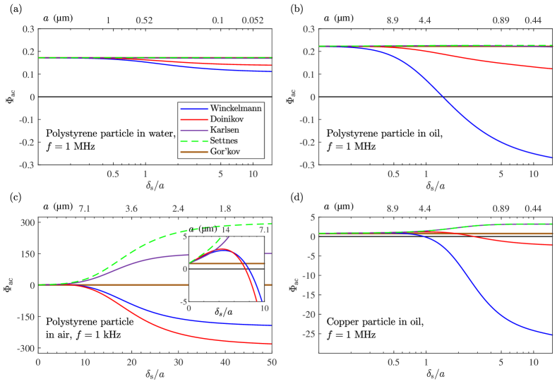
Figure 2: The acoustic contrast factor $\Phi_{\mathrm{ac}}$ plotted versus normalized boundary-layer width $\delta_{s}/a$. Brown lines are the ideal-fluid theory following Gor’kov [3]. Green dashed lines are from Settnes and Bruus [9], magenta lines are from Karlsen and Bruus [10], red lines are from Doinikov 1997 [7], and blue lines are the present theory by Winckelmann and Bruus. (a) A polystyrene sphere in water at frequency $f=1$ MHz. (b) A polystyrene sphere in oil at $f=1$ MHz. (c) A polystyrene sphere in air at $f=1$ kHz. The inset shows the large-particle behavior. (d) A copper sphere in oil at $f=1$ MHz.

Table 2: Parameters for the four combinations of solid particles in fluids discussed in Section VII.1 and shown in Fig. 2 for the cases (a) polystyrene in water, (b) polystyrene in oil, (c) polystyrene in air, and (d) copper in oil.

Case	Ref.	(a)	(b)	(c)	(d)
$\tilde{\rho}_{0}-1$	Eq. (41)	0.05	0.14	903	8.7
$\tilde{\kappa}_{s0}$	Eq. (41)	0.53	0.46	$3\times 10^{-5}$	0.01
$B_{c}$	Eq. (89a)	1.2	9.5	$-$0.30	9.5
$\gamma_{0}-1$	Eq. (5b)	0.012	0.15	0.40	0.15

boundary-layer theories converge towards the ideal-fluid result by Gor’kov for all cases. For a small particle, $a\lesssim\delta_{s}$, significant thermoviscous corrections to the ideal-fluid theory arise. We observe that the corrections found by each theory are most pronounced for a large relative density contrast $\tilde{\rho}_{0}-1$. Case (a) of polystyrene in water with $\tilde{\rho}_{0}-1=0.05$ shown in Fig. 2(a) illustrates this point, as we see less dramatic corrections from the ideal-fluid theory compared to the three other solid-fluid combinations, only a modest 30-% decrease for the smallest 50-nm-radius particles. It is clearly seen from cases (b)-(d) with $\tilde{\rho}_{0}-1=0.14$, 903 and 8.7 that the microstreaming included by Doinikov and Winckelmann becomes dominant for small particles, in agreement with the recent numerical study by Pavlic et al. [49]. The results by Doinikov and Winckelmann exhibit the same qualitative behavior, but significant quantitative discrepancies between the two microstreaming models develop, when the temperature dependency of the viscosity, included by Winckelmann through the fluid parameter $B_{c}$, is large. This discrepancy is particularly large in cases (b) and (d) both having $B_{c}=9.5$, but less prominent for cases (a) and (c) with $B_{c}=1.2$ and $-$0.30, respectively.

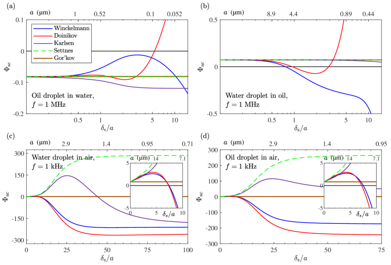
Figure 3: The acoustic contrast factor $\Phi_{\mathrm{ac}}$ plotted versus normalized boundary-layer thickness $\delta_{s}/a$. Brown lines are the ideal-fluid theory following Gor’kov [3]. Green dashed lines are from Settnes and Bruus [9], magenta lines are from Karlsen and Bruus [10], red lines are from Doinikov 1997 [8], and blue lines are the present theory by Winckelmann and Bruus. (a) An oil droplet in water at frequency $f=1$ MHz. (b) A water droplet in oil at $f=1$ MHz. (c) A water droplet in air at $f=1$ kHz. (d) An oil droplet in air at $f=1$ kHz. The insets in (c) and (d) show the large-particle behavior.

We add the following specific comments to cases (b)-(d) in Fig. 2: In case (b) it is noteworthy that the full thermoviscous model by Winckelmann for a polystyrene particle in oil at $1~{}\textrm{MHz}$, in contrast to Doinikov’s model, predicts a sign reversal of the acoustic contrast factor $\Phi_{\mathrm{ac}}$, and that this happens at a relatively large particle radius $a=3.1~{}\textrm{\textmu{}m}$. In case (c), a polystyrene particle in air at $1~{}\textrm{kHz}$, both Doinikov’s and Winckelman’s model predict a strong thermoviscous response, including a sign reversal in $\Phi_{\mathrm{ac}}$ for relatively large particles at nearly the same radius $a=9.5~{}\textrm{\textmu{}m}$ and $a=9.0~{}\textrm{\textmu{}m}$, respectively. Finally, case (d) with a copper sphere in oil at $1~{}\textrm{MHz}$ was treated more in depth in a numerical study by Baasch, Pavlic, and Dual [21]. They found a remarkable sign reversal in $\Phi_{\mathrm{ac}}$ at a relatively large particle radius $a$, and they furthermore showed that this was correctly predicted by the viscous rigid-solid theory by Doinikov [5]. Qualitatively, we confirm this sign reversal, but quantitatively we find it to happen for $a=4.7~{}\textrm{\textmu{}m}$, which is nearly three times the value $1.6~{}\textrm{\textmu{}m}$ predicted by the Doinikov model. Moreover, by including the temperature dependency of the viscosity, we find that at the smallest particle radius $a=300$ nm, $\Phi_{\mathrm{ac}}$ is an order of magnitude larger than predicted by the Doinikov model.

VII.2 The contrast factor for fluid particles

We now replace the solid particle by a fluid particle, and study the following four examples of spherical microdroplets in fluids: (a) An oil droplet in water, (b) a water droplet in oil, (c) a water droplet in air, and (d) an oil droplet in air, with material parameters listed in Tables 1 and 3. Cases (a) and (b) are chosen for their relevance to studies of droplets and emulsions [37, 38, 50]. Cases (c) and (d) are chosen for their relevance for aerosol studies [39]. In Fig. 3 we plot $\Phi_{\mathrm{ac}}$ versus $\delta_{s}/a$ computed from Eq. (109c) (blue full curve “Winckelmann”) for these four cases and compare with the results for $\Phi_{\mathrm{ac}}$ obtained by Doinikov [8] (red full curve “Doinikov”), Karlsen and Bruus [10] (purple full curve “Karlsen”), Settnes and Bruus [9] (green dashed curve “Settnes”), and Gor’kov [3] (brown full curve “Gor’kov”). As for solid particles, we see that for large fluid particles, $a\gg\delta_{s}$, the four boundary-layer theories converge towards the ideal-fluid result by Gor’kov for all cases.

Table 3: Parameters for the four combinations of fluid particles in fluids discussed in Section VII.2 and shown in Fig. 3 for the cases (a) oil in water, (b) water in oil, (c) water in air, and (d) oil in air.

Case	(a)	(b)	(c)	(d)
$\tilde{\rho}_{0}-1$	$-$0.07	0.08	857	794
$\tilde{\kappa}_{s0}$	1.17	0.86	$6\times 10^{-5}$	$7\times 10^{-5}$
$\tilde{\eta}_{0}$	67	0.015	46	$3.1\times 10^{3}$
$B_{c}$	1.2	9.5	$-$0.30	$-$0.30
$B_{t}$	$-$81	$-$63	0.75	0.75
$B^{\prime}_{t}$	$-$63	$-$81	$-$81	$-$63
$\gamma_{0}-1$	0.012	0.15	0.40	0.40
$\gamma_{\mathrm{surf}}$	$38\>$mN$\>\textrm{m}^{-1}$	$38\>$mN$\>\textrm{m}^{-1}$	$72\>$mN$\>\textrm{m}^{-1}$	$22\>$mN$\>\textrm{m}^{-1}$

Case (a), an oil droplet in water, is shown in Fig. 3(a). Here, Karlsen predicted an approximate doubling of $\Phi_{\mathrm{ac}}$ compared to the ideal-fluid theory. By adding microstreaming, Doinikov and Winckelmann also predict large variations from the ideal theory, but in contrast to the solid-particle cases, the two microstreaming models behave qualitatively different for small particles. We find that the sharp increase of $\Phi_{\mathrm{ac}}$ for $\delta_{s}/a\gtrsim 2$ given by the Doinikov model is an artifact, which is due to the previously mentioned neglect of the tangential component $s_{1\theta}$ of the displacement $\bm{s}_{1}$ in the Stokes terms in Eqs. (72) and (77) combined with the effects of surface tension in the scattering coefficients. The downwards slope in the curve by Winckelmann for $\delta_{s}/a\gtrsim 2$ stems from a combination of surface tension and the inclusion of streaming inside the fluid droplet. The temperature dependency of the viscosities only make slight quantitative contributions to the behavior of the curve by Winckelmann.

In case (b), a water droplet suspended in oil shown in Fig. 3(b), the Doinikov and the Winckelmann model have a similar behavior as in case (a), namely an increase and a decrease, respectively, of $\Phi_{\mathrm{ac}}$ for $\delta_{s}/a\gtrsim 2$. The stronger decrease of $\Phi_{\mathrm{ac}}$ in the Winckelmann model setting in at $\delta_{s}/a\gtrsim 5$ is due to inner streaming not included in the Doinikov model. In contrast to case (a), the microstreaming models in case (b) exhibit a sign change of $\Phi_{\mathrm{ac}}$, and for both models this happens at nearly the same particle size $a\approx\delta_{s}$. The sharp increase in $\Phi_{\mathrm{ac}}$ predicted by Doinikov is again due to the neglect of some of the Stokes terms as discussed before, while surface tension plays a minor role for the curves by Doinikov and Winckelmann in case (b). Like in case (a), temperature dependencies in the viscosities lead to quantitative changes to the curve by Winckelmann. Comparing Fig. 2(b), Fig. 2(d), and Fig. 3(b), we note that the Winckelmann model predicts the sign change in $\Phi_{\mathrm{ac}}$ to happen at $a\approx\delta_{s}$ for polystyrene, copper, and water particles in oil. Finally, we note that also the Karlsen-model predicts a sign change of $\Phi_{\mathrm{ac}}$ for a water droplet in oil, but this happens for much smaller particles of size $a\approx 0.04\delta_{s}$, not shown. Clearly, microstreaming is dominating the behavior of $\bm{F}^{\mathrm{rad}}$ for microparticles with $a\lesssim\delta_{s}$ and a density ratio $\tilde{\rho}_{0}$ deviating sufficiently from unity.

Case (c) of a water droplet in air shown in Fig. 3(c) was studied by Karlsen [10], who found a remarkable sign reversal in $\Phi_{\mathrm{ac}}$. For an acoustic frequency of $1~{}\textrm{kHz}$, this sign reversal happens for relatively large droplets of radius $a\approx 1.6~{}\textrm{\textmu{}m}$ surrounded by a thick boundary layer with $\delta_{s}\approx 45a$. Adding microstreaming, a corresponding sign reversal is also found by both Doinikov and Winckelmann, albeit for significantly larger particles, $a\approx 9.7~{}\textrm{\textmu{}m}$. In this case, the discrepancy between Doinikov and Winckelmann is minute, due to a small value of $B_{c}=-0.3$ and a large value of $\tilde{\eta}_{0}=46$, making this case similar to the solid-particle-in-air case in Fig. 2(c).

Case (d) with an oil droplet in air shown in Fig. 3(d) exhibits similar qualitative behavior as for the water droplet in case (c) for four of the five models. The exception is the Karlsen model, where no sign reversal occurs in $\Phi_{\mathrm{ac}}$ for the oil droplet, in contrast to the sign reversal in $\Phi_{\mathrm{ac}}$ at $\delta\approx 45a$ for the water droplet. The microstreaming models by Doinikov and Winckelmann predict a sign reversal in $\Phi_{\mathrm{ac}}$ for relatively large oil droplets with $a\approx 9.9~{}\textrm{\textmu{}m}$ and $a\approx 9.5~{}\textrm{\textmu{}m}$, respectively, close to the value $a\approx 9.7~{}\textrm{\textmu{}m}$ found above for water droplets.

We do not cover the case of gas bubbles in a surrounding fluids for several reasons. Bubble dynamics often involves nonlinearities and cavitation effects [51, 52], as well as gas diffusion across the interface [53], effects that are not included in our work. Also, in microfluidic experiments, bubbles are typically stabilized by surface coatings, which alters the bubble dynamics [51] and requires the addition of extra terms in the boundary conditions to describe the surface coating. But we do expect our model to be accurate for large bubbles in weak acoustic fields, where surface effects and nonlinearities are negligible.

VII.3 Rigidified droplets

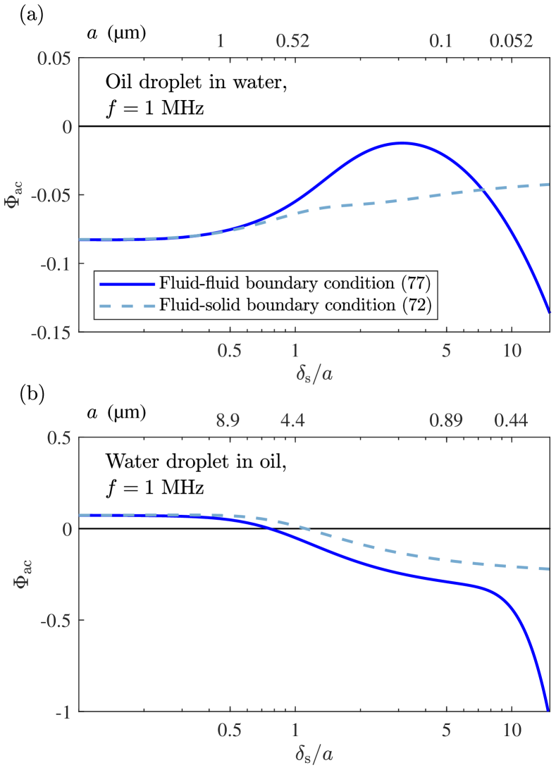
Figure 4: The acoustic contrast factor $\Phi_{\mathrm{ac}}$ from Eq. (109c) plotted versus $\delta_{s}/a$ computed for a fluid particle in a fluid using the fluid-fluid boundary condition (77) (full curve) and the fluid-solid boundary condition (72) (dashed curve). (a) An oil droplet in water at frequency $f=1$ MHz. (b) A water droplet in oil at $f=1$ MHz.

Impurities tend to collect at fluid-fluid interfaces, which can make the interface resemble that of a rigid boundary [54]. It is also often desired to use surfactants to stabilize suspended droplets [55, 56]. Our result for $\bm{F}^{\mathrm{rad}}$ in Eq. (100) for fluid particles in fluids, is derived for pure fluid-fluid interfaces under ideal conditions. A detailed description of impure interfaces and their complex dynamics is beyond the scope of this work, but in the following we discuss how to compute $\bm{F}^{\mathrm{rad}}$ on a fluid droplet with a rigidified interface in a simplified model. For a rigidified interface, which is strong enough to impose a no-slip boundary condition on the acoustic streaming, the fluid-fluid boundary condition (77) is replaced by the fluid-solid boundary condition (72). This is equivalent to using the theory (100) for solid particles, but with the scattering coefficients $\alpha_{i,n}$ from Appendix B for solids particles replaced by $\alpha_{i,n}$ from Appendix C for fluid particles with $i=0,1,2,3$. In Fig. 4, we show the result of computing $\Phi_{\mathrm{ac}}$ from Eq. (109c) in this manner (dashed curves) compared to $\Phi_{\mathrm{ac}}$ computed for a pure fluid-fluid interface (full curves) for the two cases Fig. 4(a) an oil droplet in water and Fig. 4(b) a water droplet in oil, corresponding to the pure fluid-fluid cases of Fig. 3(a) and (b). It is seen that when assuming a rigidified interface, $\Phi_{\mathrm{ac}}$ undergoes qualitative and quantitative changes in both cases. We note that the dashed curves in Fig. 4 for $\Phi_{\mathrm{ac}}$ in rigidified droplets have a quantitatively similar behavior to that found for $\Phi_{\mathrm{ac}}$ in the Winckelmann model for solids shown in Fig. 2.

Furthermore, we remark that $\Phi_{\mathrm{ac}}$ for rigidified oil in water (dashed curve) Fig. 4(a) resembles $-\Phi_{\mathrm{ac}}$ for polystyrene in water Fig. 2(a), which can be explained by $\tilde{\kappa}_{s0}-1>1$ for oil in water, whereas $\tilde{\kappa}_{s0}-1<1$ for polystyrene in water. In contrast, we remark that $\Phi_{\mathrm{ac}}$ for rigidified water in oil (dashed curve) Fig. 4(b) resembles $+\Phi_{\mathrm{ac}}$ for polystyrene in oil Fig. 2(b), because here $\tilde{\kappa}_{s0}-1>1$ in both cases. Finally, we note that the two remaining fluid-fluid cases studied in Fig. 3(c) and (d) are only affected to a negligible degree by rigidified interfaces, and therefore they are not shown in this discussion.

VIII Conclusion

We have developed an extension of the model of the acoustic radiation force $\bm{F}^{\mathrm{rad}}$ presented by Doinikov in 1997 [7, 6, 8] for a rigid and for a fluid spherical particle suspended in a thermoviscous fluid. Our extension comprises the inclusion of (1) elastic instead of rigid solid particles, (2) temperature- and density-dependent material parameters, in particular the viscosity, (3) the tangential part of the Stokes drift in the boundary condition of the acoustic streaming on the particle surface, and (4) inner streaming in a fluid particle. Using the method of Karlsen and Bruus [10] in Section III to compute the first-order fields and that of Doinikov [4, 5] in Section IV to compute the second-order fields, we arrive in Eq. (84) at $\bm{F}^{\mathrm{rad}}=\bm{F}^{\mathrm{rad}}_{11}+\bm{F}^{\mathrm{rad}}_{2,\mathrm{in}}$, where $\bm{F}^{\mathrm{rad}}_{2,\mathrm{in}}$ is the trivial Stokes drag force due to the streaming velocity of the incoming field, and $\bm{F}^{\mathrm{rad}}_{11}$ is the force in terms of the force coefficients $D_{n}$ due to time-averaged products of the first-order acoustic fields given by Eqs. (90) and (91) for solid and fluid particles, respectively. The main result of our work is the long-wavelength limit of $\bm{F}^{\mathrm{rad}}$ presented in Eq. (100).

In Section VI we compute the force coefficients $D_{0}$ and $D_{1}$ analytically in the limit of very thin and very thick boundary layers, and compare our results with results in the literature. We verify that we obtain the same result as Doinikov [6, 7, 8] when the differences in the above-mentioned model assumptions are negligible. Using Eqs. (V.3) and (96) allows for direct comparison to the models without microstreaming, namely the thermoviscous model by Karlsen and Bruus [10], the viscous model by Settnes and Bruus [9], and the ideal-fluid model by Gor’kov [3]. We recover the results of these models for particles much larger than the acoustic boundary-layer width, but find large deviations for certain parameter values (in particular for $\tilde{\rho}_{0}\gg 1$) in the opposite limit. We thus conclude, in agreement with Doinikov for thermoviscous fluids and with recent numerical studies by Baasch, Pavlic, and Dual [21] for viscous fluids, that microstreaming can dominate the acoustic radiation force $\bm{F}^{\mathrm{rad}}$ for small particles.

Further comparisons between the above five models are carried out in Sections VII.1 and VII.2 for the important special case of a standing incident wave by plotting the acoustic contrast factor $\Phi_{\mathrm{ac}}$ of Eq. (109c) versus the normalized viscous boundary layer thickness $\delta_{s}/a$ for selected choices of particles and fluids. For the four solid-in-fluid examples (a) polystyrene in water, (b) polystyrene in oil, (c) polystyrene in air, and (d) copper in oil, shown in Fig. 2, the two main observations are: (1) The large values in (c) and (d) of the relative density contrast $\tilde{\rho}_{0}-1$ result in large thermoviscous deviations from the ideal-fluid Gor’kov model, and even in a sign reversal if microstreaming is included (the Doinikov and the Winckelmann models). (2) The two models including microstreaming exhibit the same qualitative trends, but quantitatively they differ significantly as shown for solid particles in oil in (b) and (d), where the Winckelmann model predicts a sign reversal for relatively large particle radii due to the inclusion of the temperature-dependency of the viscosity. For the four fluid-in-fluid examples (a) oil in water, (b) water in oil, (c) water in air, and (d) oil in air, shown in Fig. 3, the two main observations are: (3) Each model predicts largely the same $\Phi_{\mathrm{ac}}$ for droplets in air (c) and (d) as for solid particles in air, except for the Karlsen model. (4) The Winckelmann model deviates qualitatively from the Doinikov model for droplets in liquids (a) and (b), due to our inclusion of the tangential Stokes drift boundary condition and the inner streaming.

Finally, we have in Section VII.3 briefly addressed how to analyze the experimentally important case of droplets with rigidified surfaces due to impurities or surfactants, by combining fluid-fluid scattering coefficients with a second-order no-slip boundary condition. In Fig. 4 is shown for oil-in-water and water-in-oil systems, how the response of a rigidified droplet resembles that of an elastic solid particle.

We have extended the basic analytical theory of the acoustic radiation force on a single suspended particle by including temperature- and density dependent material parameters and by taking inner streaming in droplets into account. We have shown specific examples where these effects are important. We hope that our analysis will inspire related experimental efforts in the fields of microscale acoustofluidics, acoustic levitation, and aerosol dynamics.

Appendix A Integrals of Legendre polynomials

Below, we list a series of useful integrals containing products of Legendre polynomials and their derivatives [57],

$$\int_{0}^{\pi}P_{n}(\cos\theta)P_{m}(\cos\theta)\sin\theta\,\mathrm{d}\theta =\frac{2}{2n+1}\delta_{mn}$$ (111a)

$$\int_{0}^{\pi}\partial_{\theta}P_{n}(\cos\theta)\partial_{\theta}P_{m}(\cos\theta)\sin\theta\,\mathrm{d}\theta =\frac{2n(n+1)}{2n+1}\delta_{mn}$$ (111b)

$$\int_{0}^{\pi}P_{n}(\cos\theta)P_{m}(\cos\theta)\cos\theta\sin\theta\,\mathrm{d}\theta =\begin{cases}\frac{2(n+1)}{(2n+1)(2n+3)}&m=n+1\\ \frac{2n}{(2n-1)(2n+1)}&m=n-1\\ 0&\text{otherwise}\end{cases}$$ (111c)

$$\int_{0}^{\pi}P_{n}(\cos\theta)\partial_{\theta}P_{m}(\cos\theta)\sin^{2}\theta\,\mathrm{d}\theta =\begin{cases}-\frac{2(n+1)(n+2)}{(2n+1)(2n+3)}&m=n+1\\ \frac{2(n-1)n}{(2n-1)(2n+1)}&m=n-1\\ 0&\text{otherwise}\end{cases}$$ (111d)

$$\int_{0}^{\pi}\partial_{\theta}P_{n}(\cos\theta)\partial_{\theta}P_{m}(\cos\theta)\cos\theta\sin\theta\,\mathrm{d}\theta =\begin{cases}\frac{2n(n+1)(n+2)}{(2n+1)(2n+3)}&m=n+1\\ \frac{2(n-1)n(n+1)}{(2n-1)(2n+1)}&m=n-1\\ 0&\text{otherwise}\end{cases}$$ (111e)

$$\int_{0}^{\pi}\partial_{\theta}P_{n}(\cos\theta)\partial_{\theta}^{2}P_{m}(\cos\theta)\sin^{2}\theta\,\mathrm{d}\theta =\begin{cases}-\frac{2n(n+1)(n+2)^{2}}{(2n+1)(2n+3)}&m=n+1\\ \frac{2(n-1)^{2}n(n+1)}{(2n-1)(2n+1)}&m=n-1\\ 0&\text{otherwise}\end{cases}$$ (111f)

Appendix B Scattering coefficients for solids

Here, we present the analytical expressions of the acoustic scattering coefficients $\alpha_{i,n}$, $i=0,1,2,3$ and $n=0,1,2$ for solid particles. Only the coefficients that contribute to $\bm{F}^{\mathrm{rad}}$ to leading order in $x_{0}$ are given explicitly, whereas only the order in $x_{0}$ is stated for the remaining coefficients, which are $\alpha^{\mathrm{sc}}_{\mathrm{t},1}$ and $\alpha^{\mathrm{sc}}_{\mathrm{t},2}$,

$$\alpha_{0,n}=1,$$ (112)

$$\alpha^{\mathrm{sc}}_{\mathrm{c},0}=-\frac{\mathrm{i}x_{\mathrm{c}}^{3}}{3}\frac{(1-\tilde{\kappa}_{s0})+3(\gamma_{0}-1)\Big{[}\Big{(}1-\frac{\tilde{\alpha}_{p0}}{\tilde{\rho}_{0}\tilde{c}_{p0}}\Big{)}\Big{(}1-\frac{\chi^{\prime}\tilde{\alpha}_{p0}}{\tilde{\rho}_{0}\tilde{c}_{p0}}\Big{)}-\frac{4}{3}\frac{\chi^{\prime}\tilde{\alpha}_{p0}\tilde{\kappa}_{s0}}{\tilde{c}_{p0}}\frac{c_{\mathrm{tr0}}^{\prime 2}}{c_{0}^{2}}\Big{(}1-\frac{\tilde{\alpha}_{p0}}{\tilde{\rho}_{0}\tilde{c}_{p0}\tilde{\kappa}_{s0}}\Big{)}\Big{]}H(x_{\mathrm{t}},x_{\mathrm{t}}^{\prime})}{1+4(\gamma_{0}-1)\frac{\chi^{\prime}\tilde{\alpha}_{p0}^{2}c_{\mathrm{tr0}}^{\prime 2}}{\tilde{\rho}_{0}\tilde{c}_{p0}^{2}c_{0}^{2}}H(x_{\mathrm{t}},x_{\mathrm{t}}^{\prime})},$$ (113)

$$\alpha^{\mathrm{sc}}_{\mathrm{t},0}=-\frac{x_{\mathrm{c}}^{2}x_{\mathrm{t}}}{\mathrm{i}+x_{\mathrm{t}}}\frac{(\gamma_{0}-1)\Big{(}1-\frac{\tilde{\alpha}_{p0}}{\tilde{\rho}_{0}\tilde{c}_{p0}}\Big{)}H(x_{\mathrm{t}},x_{\mathrm{t}}^{\prime})\mathrm{e}^{-\mathrm{i}x_{\mathrm{t}}}}{1+4(\gamma_{0}-1)\frac{\chi^{\prime}\tilde{\alpha}_{p0}^{2}c_{\mathrm{tr0}}^{\prime 2}}{\tilde{\rho}_{0}\tilde{c}_{p0}^{2}c_{0}^{2}}H(x_{\mathrm{t}},x_{\mathrm{t}}^{\prime})},$$ (114)

$$\alpha^{\mathrm{sc}}_{\mathrm{c},1}=-\frac{\mathrm{i}x_{\mathrm{c}}^{3}}{3}\frac{(\tilde{\rho}_{0}-1)(3-3\mathrm{i}x_{\mathrm{s}}-x_{\mathrm{s}}^{2})}{x_{\mathrm{s}}^{2}(2\tilde{\rho}_{0}+1)-9(1-\mathrm{i}x_{\mathrm{s}})},\quad\alpha^{\mathrm{sc}}_{\mathrm{t},1}\sim\mathcal{O}(x_{0}^{3}),\quad\alpha^{\mathrm{sc}}_{\mathrm{s},1}=\frac{\mathrm{i}x_{\mathrm{c}}(\tilde{\rho}_{0}-1)x_{\mathrm{s}}^{2}\mathrm{e}^{-\mathrm{i}x_{\mathrm{s}}}}{x_{\mathrm{s}}^{2}(2\tilde{\rho}_{0}+1)-9(1-\mathrm{i}x_{\mathrm{s}})},$$ (115)

$$\alpha^{\mathrm{sc}}_{\mathrm{c},2}=\frac{2\mathrm{i}x_{\mathrm{c}}^{5}}{135x_{\mathrm{s}}^{2}}\frac{15(1-\mathrm{i}x_{\mathrm{s}})-6x_{\mathrm{s}}^{2}+\mathrm{i}x_{\mathrm{s}}^{3}}{\mathrm{i}x_{\mathrm{s}}-1},\quad\alpha^{\mathrm{sc}}_{\mathrm{t},2}\sim\mathcal{O}(x_{0}^{4}),\quad\alpha^{\mathrm{sc}}_{\mathrm{s},2}=-\frac{\mathrm{i}x_{\mathrm{c}}^{2}}{9}\frac{x_{\mathrm{s}}\mathrm{e}^{-\mathrm{i}x_{\mathrm{s}}}}{\mathrm{i}x_{\mathrm{s}}-1},$$ (116)

$$\text{with the definition }\;H(x_{\mathrm{t}},x_{\mathrm{t}}^{\prime})=\frac{1}{x_{\mathrm{t}}^{2}}\bigg{[}\frac{1}{1-\mathrm{i}x_{\mathrm{t}}}-\frac{1}{\tilde{k}^{\mathrm{th}}_{0}}\frac{\tan x_{\mathrm{t}}^{\prime}}{\tan x_{\mathrm{t}}^{\prime}-x_{\mathrm{t}}^{\prime}}\bigg{]}^{-1}.$$ (117)

Appendix C Scattering coefficients for fluids

Here, we present the analytical expressions of the acoustic scattering coefficients $\alpha_{i,n}$, $i=0,1,2,3,4,5,6$ and $n=0,1,2$ for fluid particles. As above, only the coefficients that contribute to $\bm{F}^{\mathrm{rad}}$ to leading order in $x_{0}$ are given explicitly, while only the order in $x_{0}$ is stated for the remaining coefficients, which are $\alpha^{\mathrm{sc}}_{\mathrm{t},1}$, $\alpha_{\mathrm{t},1}^{\prime}$, $\alpha^{\mathrm{sc}}_{\mathrm{t},2}$, and $\alpha_{\mathrm{t},2}^{\prime}$,

$$\alpha_{0,n}=1,$$ (118)

$$\alpha^{\mathrm{sc}}_{\mathrm{c},0}=-\frac{\mathrm{i}x_{\mathrm{c}}^{3}}{3}\frac{1-\tilde{\kappa}_{s0}+3(\gamma_{0}-1)\Big{(}1-\frac{\tilde{\alpha}_{p0}}{\tilde{\rho}_{0}\tilde{c}_{p0}}\Big{)}^{2}H(x_{\mathrm{t}},x_{\mathrm{t}}^{\prime})-\frac{2\gamma_{\mathrm{surf}}\kappa_{s0}^{\prime}}{3a}\Big{[}1+3(\gamma_{0}-1)\Big{(}1-\frac{\tilde{\alpha}_{p0}^{2}}{\tilde{\rho}_{0}^{2}\tilde{c}_{p0}^{2}\tilde{\kappa}_{s0}}\Big{)}H(x_{\mathrm{t}},x_{\mathrm{t}}^{\prime})\Big{]}}{1-\frac{2\gamma_{\mathrm{surf}}\kappa_{s0}^{\prime}}{3a}\Big{[}1-3(\gamma_{0}-1)\frac{\tilde{\alpha}_{p0}^{2}}{\tilde{\rho}_{0}^{2}\tilde{c}_{p0}^{2}\tilde{\kappa}_{s0}}H(x_{\mathrm{t}},x_{\mathrm{t}}^{\prime})\Big{]}},$$ (119)

$$\alpha^{\mathrm{sc}}_{\mathrm{t},0}=-\frac{x_{\mathrm{c}}^{2}x_{\mathrm{t}}}{\mathrm{i}+x_{\mathrm{t}}}\frac{(\gamma_{0}-1)\Big{[}\Big{(}1-\frac{\tilde{\alpha}_{p0}}{\tilde{\rho}_{0}\tilde{c}_{p0}}\Big{)}-\frac{2\gamma_{\mathrm{surf}}\kappa_{s0}^{\prime}}{3a}\Big{]}H(x_{\mathrm{t}},x_{\mathrm{t}}^{\prime})\mathrm{e}^{-\mathrm{i}x_{\mathrm{t}}}}{1-\frac{2\gamma_{\mathrm{surf}}\kappa_{s0}^{\prime}}{3a}\Big{[}1-3(\gamma_{0}-1)\frac{\tilde{\alpha}_{p0}^{2}}{\tilde{\rho}_{0}^{2}\tilde{c}_{p0}^{2}\tilde{\kappa}_{s0}}H(x_{\mathrm{t}},x_{\mathrm{t}}^{\prime})\Big{]}},\quad\alpha_{\mathrm{c},0}^{\prime}=\frac{\tilde{\rho}_{0}^{-1}+(\gamma_{0}-1)\frac{2\gamma_{\mathrm{surf}}\kappa_{s0}^{\prime}}{a}\frac{\tilde{\alpha}_{p0}}{\tilde{\rho}_{0}^{2}\tilde{c}_{p0}\tilde{\kappa}_{s0}}H(x_{\mathrm{t}},x_{\mathrm{t}}^{\prime})}{1-\frac{2\gamma_{\mathrm{surf}}\kappa_{s0}^{\prime}}{3a}\Big{[}1-3(\gamma_{0}-1)\frac{\tilde{\alpha}_{p0}^{2}}{\tilde{\rho}_{0}^{2}\tilde{c}_{p0}^{2}\tilde{\kappa}_{s0}}H(x_{\mathrm{t}},x_{\mathrm{t}}^{\prime})\Big{]}},$$ (120)

$$\alpha_{\mathrm{t},0}^{\prime}=\frac{x_{\mathrm{c}}^{2}x_{\mathrm{t}}^{\prime}}{\sin x_{\mathrm{t}}^{\prime}-x_{\mathrm{t}}^{\prime}\cos x_{\mathrm{t}}^{\prime}}\frac{(\gamma_{0}-1)\frac{\tilde{\alpha}_{p0}}{\tilde{\rho}_{0}\tilde{c}_{p0}}\Big{[}\Big{(}1-\frac{\tilde{\alpha}_{p0}}{\tilde{\rho}_{0}\tilde{c}_{p0}}\Big{)}-\frac{2\gamma_{\mathrm{surf}}\kappa_{s0}^{\prime}}{3a}\Big{]}H(x_{\mathrm{t}},x_{\mathrm{t}}^{\prime})}{1-\frac{2\gamma_{\mathrm{surf}}\kappa_{s0}^{\prime}}{3a}\Big{[}1-3(\gamma_{0}-1)\frac{\tilde{\alpha}_{p0}^{2}}{\tilde{\rho}_{0}^{2}\tilde{c}_{p0}^{2}\tilde{\kappa}_{s0}}H(x_{\mathrm{t}},x_{\mathrm{t}}^{\prime})\Big{]}},$$ (121)

$$\alpha^{\mathrm{sc}}_{\mathrm{c},1}=\frac{\mathrm{i}x_{\mathrm{c}}^{3}}{3}\frac{(\tilde{\rho}_{0}-1)[1+F(x_{\mathrm{s}},x_{\mathrm{s}}^{\prime})-G(x_{\mathrm{s}})]}{(2\tilde{\rho}_{0}+1)[1+F(x_{\mathrm{s}},x_{\mathrm{s}}^{\prime})]-3G(x_{\mathrm{s}})},\qquad\alpha^{\mathrm{sc}}_{\mathrm{t},1}\sim\mathcal{O}(x_{0}^{3}),\qquad\alpha^{\mathrm{sc}}_{\mathrm{s},1}=\frac{\mathrm{i}x_{\mathrm{c}}(\tilde{\rho}_{0}-1)\mathrm{e}^{-\mathrm{i}x_{\mathrm{s}}}}{(2\tilde{\rho}_{0}+1)[1+F(x_{\mathrm{s}},x_{\mathrm{s}}^{\prime})]-3G(x_{\mathrm{s}})},$$ (122)

$$\alpha_{\mathrm{c},1}^{\prime}=\frac{3x_{\mathrm{c}}}{x_{\mathrm{c}}^{\prime}}\frac{1-\frac{2+\tilde{\rho}_{0}}{3\tilde{\rho}_{0}}G(x_{\mathrm{s}})+F(x_{\mathrm{s}},x_{\mathrm{s}}^{\prime})\Big{[}1+\frac{4}{\tilde{\rho}_{0}x_{\mathrm{s}}^{2}}(\tilde{\rho}_{0}-1)(\tilde{\eta}_{0}-1)\Big{]}}{(2\tilde{\rho}_{0}+1)[1+F(x_{\mathrm{s}},x_{\mathrm{s}}^{\prime})]-3G(x_{\mathrm{s}})},\quad\alpha_{\mathrm{t},1}^{\prime}\sim\mathcal{O}(x_{0}^{3}),$$ (123)

$$\alpha_{\mathrm{s},1}^{\prime}=\frac{x_{\mathrm{c}}}{x_{\mathrm{s}}^{\prime}j_{2}(x_{\mathrm{s}}^{\prime})}\frac{(\tilde{\rho}_{0}-1)F(x_{\mathrm{s}},x_{\mathrm{s}}^{\prime})}{(2\tilde{\rho}_{0}+1)[1+F(x_{\mathrm{s}},x_{\mathrm{s}}^{\prime})]-3G(x_{\mathrm{s}})},$$ (124)

$$\alpha^{\mathrm{sc}}_{\mathrm{c},2}=-\frac{\mathrm{i}x_{\mathrm{c}}^{5}x_{\mathrm{s}}}{45}\frac{32(\tilde{\eta}_{0}-1)^{2}-2x_{\mathrm{s}}^{2}(\tilde{\eta}_{0}-1)(\tilde{\rho}_{0}-1)+[10(\tilde{\eta}_{0}-1)-(\tilde{\rho}_{0}-1)x_{\mathrm{s}}^{2}]\kappa_{1}(x_{\mathrm{s}},x_{\mathrm{s}}^{\prime})+\frac{2\mathrm{i}\gamma_{\mathrm{surf}}}{\eta_{0}a\omega}[8(\tilde{\eta}_{0}-1)+4\kappa_{1}(x_{\mathrm{s}},x_{\mathrm{s}}^{\prime})]}{X_{1}(x_{\mathrm{s}})+\tilde{\eta}_{0}X_{2}(x_{\mathrm{s}},x_{\mathrm{s}}^{\prime})+\tilde{\eta}_{0}^{2}X_{3}(x_{\mathrm{s}},x_{\mathrm{s}}^{\prime})+\frac{2\mathrm{i}\gamma_{\mathrm{surf}}}{\eta_{0}a\omega}X_{4}(x_{\mathrm{s}},x_{\mathrm{s}}^{\prime})},$$ (125)

$$\alpha^{\mathrm{sc}}_{\mathrm{s},2}=\frac{x_{\mathrm{c}}^{2}}{6h_{3}(x_{\mathrm{s}})}\frac{(\tilde{\eta}_{0}-1)\Big{[}32(\tilde{\eta}_{0}-1)-2(\tilde{\rho}_{0}-2)x_{\mathrm{s}}^{2}\Big{]}-\tilde{\eta}_{0}\Big{[}10(\tilde{\eta}_{0}-1)-(\tilde{\rho}_{0}-1)x_{\mathrm{s}}^{2}\Big{]}\kappa_{2}(x_{\mathrm{s}}^{\prime})+\frac{2\mathrm{i}\gamma_{\mathrm{surf}}}{\eta_{0}a\omega}[8(\tilde{\eta}_{0}-1)-4\tilde{\eta}_{0}\kappa_{2}(x_{\mathrm{s}}^{\prime})]}{X_{1}(x_{\mathrm{s}})+\tilde{\eta}_{0}X_{2}(x_{\mathrm{s}},x_{\mathrm{s}}^{\prime})+\tilde{\eta}_{0}^{2}X_{3}(x_{\mathrm{s}},x_{\mathrm{s}}^{\prime})+\frac{2\mathrm{i}\gamma_{\mathrm{surf}}}{\eta_{0}a\omega}X_{4}(x_{\mathrm{s}},x_{\mathrm{s}}^{\prime})},$$ (126)

$$\alpha_{\mathrm{c},2}^{\prime}=\frac{5x_{\mathrm{c}}^{2}x_{\mathrm{s}}^{2}}{2x_{\mathrm{c}}^{\prime 2}x_{\mathrm{s}}^{\prime}}\frac{x_{\mathrm{s}}x_{\mathrm{s}}^{\prime}\kappa_{1}(x_{\mathrm{s}},x_{\mathrm{s}}^{\prime})+2(\tilde{\eta}_{0}-1)\kappa_{3}(x_{\mathrm{s}},x_{\mathrm{s}}^{\prime})+\Big{[}3x_{\mathrm{s}}^{2}(\tilde{\rho}_{0}-1)-12\frac{2\mathrm{i}\gamma_{\mathrm{surf}}}{\eta_{0}a\omega}\Big{]}\kappa_{4}(x_{\mathrm{s}},x_{\mathrm{s}}^{\prime})}{X_{1}(x_{\mathrm{s}})+\tilde{\eta}_{0}X_{2}(x_{\mathrm{s}},x_{\mathrm{s}}^{\prime})+\tilde{\eta}_{0}^{2}X_{3}(x_{\mathrm{s}},x_{\mathrm{s}}^{\prime})+\frac{2\mathrm{i}\gamma_{\mathrm{surf}}}{\eta_{0}a\omega}X_{4}(x_{\mathrm{s}},x_{\mathrm{s}}^{\prime})},$$ (127)

$$\alpha_{\mathrm{s},2}^{\prime}=\frac{x_{\mathrm{c}}^{2}x_{\mathrm{s}}^{2}}{6x_{\mathrm{s}}^{\prime}j_{3}(x_{\mathrm{s}}^{\prime})}\frac{2x_{\mathrm{s}}(\tilde{\eta}_{0}-1)+\Big{[}(\tilde{\rho}_{0}-1)x_{\mathrm{s}}^{2}-10(\tilde{\eta}_{0}-1)-4\frac{2\mathrm{i}\gamma_{\mathrm{surf}}}{\eta_{0}a\omega}\Big{]}\frac{h_{2}(x_{\mathrm{s}})}{h_{3}(x_{\mathrm{s}})}}{X_{1}(x_{\mathrm{s}})+\tilde{\eta}_{0}X_{2}(x_{\mathrm{s}},x_{\mathrm{s}}^{\prime})+\tilde{\eta}_{0}^{2}X_{3}(x_{\mathrm{s}},x_{\mathrm{s}}^{\prime})+\frac{2\mathrm{i}\gamma_{\mathrm{surf}}}{\eta_{0}a\omega}X_{4}(x_{\mathrm{s}},x_{\mathrm{s}}^{\prime})},$$ (128)

$$\alpha^{\mathrm{sc}}_{\mathrm{t},2}\sim x_{0}^{4},\qquad\alpha_{\mathrm{t},2}^{\prime}\sim x_{0}^{4}.$$ (129)

Alongside $H(x_{\mathrm{t}},x_{\mathrm{t}}^{\prime})$ from Appendix B, we have here defined the functions

$$G(x_{\mathrm{s}}) =\frac{3}{x_{\mathrm{s}}}\bigg{(}\frac{1}{x_{\mathrm{s}}}-\mathrm{i}\bigg{)},\qquad F(x_{\mathrm{s}},x_{\mathrm{s}}^{\prime})=\frac{1-\mathrm{i}x_{\mathrm{s}}}{2(1-\tilde{\eta}_{0})+\frac{\tilde{\eta}_{0}x_{\mathrm{s}}^{\prime 2}(\tan x_{\mathrm{s}}^{\prime}-x_{\mathrm{s}}^{\prime})}{(3-x_{\mathrm{s}}^{\prime 2})\tan x_{\mathrm{s}}^{\prime}-3x_{\mathrm{s}}^{\prime}}},$$ (130a)

$$X_{1}(x_{\mathrm{s}}) =(240-30x_{\mathrm{s}}^{2}+x_{\mathrm{s}}^{4})\frac{h_{2}(x_{\mathrm{s}})}{h_{3}(x_{\mathrm{s}})}-2x_{\mathrm{s}}(x_{\mathrm{s}}^{2}+24),$$ (130b)

$$X_{2}(x_{\mathrm{s}},x_{\mathrm{s}}^{\prime}) =\frac{x_{\mathrm{s}}^{\prime}j_{2}(x_{\mathrm{s}}^{\prime})}{j_{3}(x_{\mathrm{s}}^{\prime})}\Big{[}\Big{(}75-\frac{15}{2}x_{\mathrm{s}}^{2}\Big{)}\frac{h_{2}(x_{\mathrm{s}})}{h_{3}(x_{\mathrm{s}})}-x_{\mathrm{s}}(x_{\mathrm{s}}^{2}+15)\Big{]}$$

$$\quad+\bigg{[}\bigg{(}\frac{3}{2}x_{\mathrm{s}}^{\prime 2}+30\bigg{)}x_{\mathrm{s}}^{2}+15x_{\mathrm{s}}^{\prime 2}-480\bigg{]}\frac{h_{2}(x_{\mathrm{s}})}{h_{3}(x_{\mathrm{s}})}+2x_{\mathrm{s}}\Big{(}x_{\mathrm{s}}^{2}-\frac{3}{2}x_{\mathrm{s}}^{\prime 2}+48\Big{)},$$ (130c)

$$X_{3}(x_{\mathrm{s}},x_{\mathrm{s}}^{\prime}) =\frac{3[5h_{2}(x_{\mathrm{s}})-x_{\mathrm{s}}h_{3}(x_{\mathrm{s}})]}{2h_{3}(x_{\mathrm{s}})}\frac{(x_{\mathrm{s}}^{\prime 3}-10x_{\mathrm{s}}^{\prime})j_{2}(x_{\mathrm{s}}^{\prime})+(32-2x_{\mathrm{s}}^{\prime 2})j_{3}(x_{\mathrm{s}}^{\prime})}{j_{3}(x_{\mathrm{s}}^{\prime})},$$ (130d)

$$X_{4}(x_{\mathrm{s}},x_{\mathrm{s}}^{\prime}) =6\bigg{\{}\Big{[}10(\tilde{\eta}_{0}-1)-x_{\mathrm{s}}^{2}\Big{]}\frac{h_{2}(x_{\mathrm{s}})}{h_{3}(x_{\mathrm{s}})}-2x_{\mathrm{s}}(\tilde{\eta}_{0}-1)+\tilde{\eta}_{0}\frac{x_{\mathrm{s}}h_{3}(x_{\mathrm{s}})-5h_{2}(x_{\mathrm{s}})}{h_{3}(x_{\mathrm{s}})}\frac{x_{\mathrm{s}}^{\prime}j_{2}(x_{\mathrm{s}}^{\prime})}{j_{3}(x_{\mathrm{s}}^{\prime})}\bigg{\}},$$ (130e)

$$\kappa_{1}(x_{\mathrm{s}},x_{\mathrm{s}}^{\prime}) =\frac{h_{2}(x_{\mathrm{s}})x_{\mathrm{s}}}{h_{3}(x_{\mathrm{s}})}-\tilde{\eta}_{0}\frac{x_{\mathrm{s}}^{\prime}j_{2}(x_{\mathrm{s}}^{\prime})}{j_{3}(x_{\mathrm{s}}^{\prime})},\quad\quad\kappa_{2}(x_{\mathrm{s}}^{\prime})=\frac{j_{2}(x_{\mathrm{s}}^{\prime})x_{\mathrm{s}}^{\prime}}{j_{3}(x_{\mathrm{s}}^{\prime})},$$ (130f)

$$\kappa_{3}(x_{\mathrm{s}},x_{\mathrm{s}}^{\prime}) =\frac{[3x_{\mathrm{s}}h_{3}(x_{\mathrm{s}})-15h_{2}(x_{\mathrm{s}})]j_{2}(x_{\mathrm{s}}^{\prime})+[x_{\mathrm{s}}h_{3}(x_{\mathrm{s}})+3h_{2}(x_{\mathrm{s}})]x_{\mathrm{s}}^{\prime}j_{3}(x_{\mathrm{s}}^{\prime})}{h_{3}(x_{\mathrm{s}})j_{3}(x_{\mathrm{s}}^{\prime})},\quad\kappa_{4}(x_{\mathrm{s}},x_{\mathrm{s}}^{\prime})=\frac{h_{2}(x_{\mathrm{s}})j_{2}(x_{\mathrm{s}}^{\prime})}{h_{3}(x_{\mathrm{s}})j_{3}(x_{\mathrm{s}}^{\prime})}.$$ (130g)

Appendix D Derivation of Eq. (V.1) involving c${}_{\textbf{41}}$ and c${}_{\textbf{51}}$

The details of the computation leading to Eq. (V.1) involving $c_{41}$ and $c_{51}$ are given here. First, the expressions for $c_{41}$ and $c_{51}$ from Eqs. (71d) and (71e) are used to obtain,

$$-\bm{e}_{z}4\pi\rho_{0}\nu_{0}\bigg{(}\frac{3}{2}c_{51}-\frac{1}{4}c_{41}\bigg{)}=-\bm{e}_{z}2\pi\rho_{0}\nu_{0}\int_{1}^{\infty}\Big{[}3\xi-\xi^{-1}\Big{]}\Big{[}\chi_{r1}(\xi)-2\chi_{\theta 1}(\xi)\Big{]}+3\chi_{\theta 1}(\xi)\Big{[}\xi-\xi^{-1}\Big{]}\>\mathrm{d}\xi.$$ (131)

Then $\chi_{r1}(\xi)$ and $\chi_{\theta n}(\xi)$ are inserted from Eqs. (60) and (60) for $n=1$, and the second term in the integrand yields

$$-\bm{e}_{z}\>2\pi\rho_{0}\nu_{0}\int_{1}^{\infty}3\chi_{\theta 1}(\xi)(\xi-\xi^{-1})\mathrm{d}\xi=$$ (132)

$$\hskip 28.45274pt-\bm{e}_{z}3\pi\rho_{0}a^{3}\int_{1}^{\infty}\int_{0}^{\pi}\frac{1}{2}\big{[}\xi-\xi^{-1}\big{]}\bigg{\{}\bm{\nabla}\cdot\Big{\langle}\bm{v}_{1}\bm{v}_{1}-\nu_{1}\Big{[}\bm{\nabla}\bm{v}_{1}+(\bm{\nabla}\bm{v}_{1})^{\textsf{T}}\Big{]}-\Big{[}\nu_{1}^{\mathrm{b}}-\tfrac{2}{3}\nu_{1}\Big{]}(\bm{\nabla}\cdot\bm{v}_{1})\textbf{{I}}\Big{\rangle}_{\mathrm{nii}}\bigg{\}}\cdot\bm{e}_{\theta}\sin^{2}\theta\,\mathrm{d}\theta\mathrm{d}\xi.$$

To ease the notation in the following, we introduce

$$\bm{X}=\Big{\langle}\bm{v}_{1}\bm{v}_{1}-\nu_{1}\Big{[}\bm{\nabla}\bm{v}_{1}+(\bm{\nabla}\bm{v}_{1})^{\textsf{T}}\Big{]}-\Big{[}\nu_{1}^{\mathrm{b}}-\tfrac{2}{3}\nu_{1}\Big{]}(\bm{\nabla}\cdot\bm{v}_{1})\textbf{{I}}\Big{\rangle}_{\mathrm{nii}}.$$ (133a)

Using this expression for $$\bm{X}$$, the first term of the integrand in Eq. (131) becomes

$$-\bm{e}_{z}2\pi\rho_{0}\nu_{0}\int_{1}^{\infty}(3\xi-\xi^{-1})[\chi_{r1}(\xi)-2\chi_{\theta 1}(\xi)]\mathrm{d}\xi$$

$$\hskip 19.91692pt=-\bm{e}_{z}2\pi\rho_{0}\nu_{0}\frac{a^{3}}{2\nu_{0}}\int_{1}^{\infty}\int_{0}^{\pi}(3\xi-\xi^{-1})\,\big{(}\bm{\nabla}\cdot\bm{X}\big{)}\!\cdot(\bm{e}_{r}\cos\theta-\bm{e}_{\theta}\sin\theta)\sin\theta\,\mathrm{d}\theta\mathrm{d}\xi$$

$$\hskip 19.91692pt=-\bm{e}_{z}\pi\rho_{0}a^{3}\int_{1}^{\infty}\int_{0}^{\pi}(3\xi^{-1}-\xi^{-3})\,\big{(}\bm{\nabla}\cdot\bm{X}\big{)}\!\cdot\bm{e}_{z}\,\xi^{2}\sin\theta\,\mathrm{d}\theta\mathrm{d}\xi$$

$$\hskip 19.91692pt=-\bm{e}_{z}\pi\rho_{0}a^{3}\int_{1}^{\infty}\int_{0}^{\pi}\Big{\{}\bm{\nabla}\cdot\big{[}(3\xi^{-1}-\xi^{-3})\bm{X}\big{]}+\frac{3}{a}\big{(}\xi^{-2}-\xi^{-4}\big{)}\,\bm{e}_{r}\cdot\bm{X}\Big{\}}\!\cdot\bm{e}_{z}\,\xi^{2}\sin\theta\>\mathrm{d}\theta\>\mathrm{d}\xi,$$ (133b)

and by inserting the definition of $$\bm{X}$$ in the second term of the integrand in Eq. (133), we obtain

$$-\bm{e}_{z}\pi\rho_{0}a^{3}\int_{1}^{\infty}\int_{0}^{\pi}\Big{\{}\frac{3}{a}\big{(}\xi^{-2}-\xi^{-4}\big{)}\,\bm{e}_{r}\cdot\bm{X}\Big{\}}\!\cdot\bm{e}_{z}\,\xi^{2}\sin\theta\,\mathrm{d}\theta\mathrm{d}\xi$$ (133c)

$$\hskip 19.91692pt=-\bm{e}_{z}3\pi\rho_{0}a^{2}\int_{1}^{\infty}\int_{0}^{\pi}\big{[}1-\xi^{-2}\big{]}\;\bm{e}_{r}\cdot\Big{\langle}(\bm{v}_{1}\bm{v}_{1})-\nu_{1}\Big{[}\bm{\nabla}\bm{v}_{1}+(\bm{\nabla}\bm{v}_{1})^{\textsf{T}}\Big{]}-[\nu_{1}^{\mathrm{b}}-\tfrac{2}{3}\nu_{1}](\bm{\nabla}\cdot\bm{v}_{1})\textbf{{I}}\Big{\rangle}_{\mathrm{nii}}\!\cdot\bm{e}_{z}\sin\theta\,\mathrm{d}\theta\mathrm{d}\xi.$$

Lastly, using Gauss’s law, we evaluate the divergence term of the integrand in Eq. (133),

$$-\bm{e}_{z}\pi\rho_{0}a^{3}\int_{1}^{\infty}\int_{0}^{\pi}\Big{\{}\bm{\nabla}\cdot\big{[}(3\xi^{-1}-\xi^{-3})\bm{X}\big{]}\Big{\}}\!\cdot\bm{e}_{z}\,\xi^{2}\sin\theta\,\mathrm{d}\theta\mathrm{d}\xi$$

$$\hskip 19.91692pt=-\bm{e}_{z}\frac{\rho_{0}}{2}\int_{1}^{\infty}\int_{0}^{\pi}\int_{0}^{2\pi}\Big{\{}\bm{\nabla}\cdot\big{[}(3\xi^{-1}-\xi^{-3})\bm{X}\big{]}\Big{\}}\!\cdot\bm{e}_{z}\,(a\xi)^{2}\sin\theta\,\mathrm{d}\varphi\mathrm{d}\theta\,a\mathrm{d}\xi,$$

$$\hskip 19.91692pt=-\frac{\rho_{0}}{2}\int_{\Omega}\bm{\nabla}\cdot\big{[}(3\xi^{-1}-\xi^{-3})\bm{X}\big{]}\mathrm{d}V,$$

$$\hskip 19.91692pt=-\frac{\rho_{0}}{2}\oint_{\partial\Omega_{0}}(3\xi^{-1}-\xi^{-3})\bm{X}\cdot\big{(}-\bm{e}_{r}\big{)}\,\mathrm{d}S-\frac{\rho_{0}}{2}\oint_{\partial\Omega_{\infty}}(3\xi^{-1}-\xi^{-3})\bm{X}\cdot\bm{e}_{r}\,\mathrm{d}S,$$

$$\hskip 19.91692pt=\rho_{0}\oint_{\partial\Omega_{0}}\Big{\langle}\bm{v}_{1}\bm{v}_{1}-\nu_{1}\Big{[}\bm{\nabla}\bm{v}_{1}+(\bm{\nabla}\bm{v}_{1})^{\textsf{T}}\Big{]}-\Big{[}\nu_{1}^{\mathrm{b}}-\tfrac{2}{3}\nu_{1}\Big{]}(\bm{\nabla}\cdot\bm{v}_{1})\textbf{{I}}\Big{\rangle}_{\mathrm{nii}}\!\cdot\bm{e}_{r}\,\mathrm{d}S.$$ (133d)

Here, we have introduced the volume $\Omega$ between the particle surface $\partial\Omega_{0}$ and a spherical surface $\partial\Omega_{\infty}$ centered at $r=0$ with a radius going to infinity. In the last line of Eq. (133), we have used that the integrand goes to zero on $\partial\Omega_{\infty}$, and the definition of $\bm{X}$ has been reinserted. With the three result from Eqs. (132), (133c) and (133) inserted in Eq. (131), we obtain the result stated in Eq. (V.1).

Appendix E The second-order coefficients S${}_{\textit{\!{ik,n}}}$ for a solid particle in a fluid

The 16 $S_{ik,n}$ coefficients that contribute to $D_{n}$ to leading order in $x_{0}$ are stated: $9$ coefficients for $n=0$ and $7$ for $n=1$. For the remaining $16$ coefficients in modes $n=0$ and $n=1$, we only state their order in $x_{0}$ here.

$$S_{00,0} =\frac{x_{0}^{3}}{3x_{\mathrm{s}}^{2}},\qquad S_{00,1}=\frac{x_{0}^{3}}{3x_{\mathrm{s}}^{2}},\qquad S_{0c,0}=\frac{2\mathrm{i}}{3},\qquad S_{0c,1}\sim\mathcal{O}(1),\qquad S_{0t,0}\sim\mathcal{O}(x_{0}^{2}),\qquad S_{0t,1}\sim\mathcal{O}(x_{0}),$$

$$S_{0s,0} =-x_{0}^{2}\frac{2\mathrm{i}(1+B_{c})}{x_{\mathrm{s}}^{2}}\mathrm{e}^{-x_{\mathrm{s}}},\qquad S_{0s,1}\sim\mathcal{O}(x_{0}^{3}),\qquad S_{c0,0}=\frac{2\mathrm{i}}{3},\qquad S_{c0,1}=\frac{2\mathrm{i}}{3},\qquad S_{cc,0}=\frac{6}{x_{\mathrm{s}}^{2}x_{0}^{3}},\qquad S_{cc,1}=\frac{135}{x_{\mathrm{s}}^{2}x_{0}^{5}},$$

$$S_{ct,0} \sim\mathcal{O}(x_{0}^{-1}),\qquad S_{ct,1}\sim\mathcal{O}(x_{0}^{-2}),$$

$$S_{cs,0} =\frac{1}{24x_{\mathrm{s}}^{4}x_{0}}\Big{[}(-x_{\mathrm{s}}^{7}+x_{\mathrm{s}}^{6}-14x_{\mathrm{s}}^{5}+18x_{\mathrm{s}}^{4}-48x_{\mathrm{s}}^{3}-96x_{\mathrm{s}}^{2}-144x_{\mathrm{s}}-144)\mathrm{e}^{-x_{\mathrm{s}}}+E_{1}(x_{\mathrm{s}})x_{\mathrm{s}}^{6}(x_{\mathrm{s}}^{2}+12)\Big{]},$$

$$S_{cs,1} =-\frac{3\mathrm{i}}{4x_{\mathrm{s}}^{5}x_{0}^{2}}\Big{[}(-x_{\mathrm{s}}^{7}+x_{\mathrm{s}}^{6}-2x_{\mathrm{s}}^{5}+6x_{\mathrm{s}}^{4}+48x_{\mathrm{s}}^{3}+168x_{\mathrm{s}}^{2}+360x_{\mathrm{s}}+360)\mathrm{e}^{-x_{\mathrm{s}}}+E_{1}(x_{\mathrm{s}})x_{\mathrm{s}}^{8}\Big{]},$$

$$S_{t0,0} =\frac{2\mathrm{i}x_{0}}{3x_{\mathrm{t}}}\mathrm{e}^{\mathrm{i}x_{\mathrm{t}}},\qquad S_{t0,1}\sim\mathcal{O}(x_{0}^{2}),$$

$$S_{tc,0} =\frac{1}{24x_{\mathrm{t}}x_{\mathrm{s}}^{2}x_{0}^{2}}\Big{\{}-\big{[}x_{\mathrm{t}}^{4}B_{\mathrm{t}}+(x_{\mathrm{s}}^{2}+18B_{\mathrm{t}}+6)x_{\mathrm{t}}^{2}+12x_{\mathrm{s}}^{2}\big{]}x_{\mathrm{t}}^{4}E_{1}(-\mathrm{i}x_{\mathrm{t}})+\Big{[}x_{\mathrm{t}}^{7}B_{\mathrm{t}}\mathrm{i}+x_{\mathrm{t}}^{6}B_{\mathrm{t}}+(x_{\mathrm{s}}^{2}\mathrm{i}+16\mathrm{i}B_{\mathrm{t}}+6\mathrm{i})x_{\mathrm{t}}^{5}$$

$$\quad+(x_{\mathrm{s}}^{2}+12B_{\mathrm{t}}+6)x_{\mathrm{t}}^{4}+(10\mathrm{i}x_{\mathrm{s}}^{2}-12\mathrm{i}B_{\mathrm{t}}-12\mathrm{i})x_{\mathrm{t}}^{3}+(6x_{\mathrm{s}}^{2}+12B_{\mathrm{t}}-36)x_{\mathrm{t}}^{2}-144\mathrm{i}x_{\mathrm{t}}+144\Big{]}\mathrm{e}^{\mathrm{i}x_{\mathrm{t}}}\Big{\}},$$

$$S_{tc,1} \sim\mathcal{O}(x_{0}^{-3}),\qquad S_{tt,0}\sim\mathcal{O}(1),\qquad S_{tt,1}\sim\mathcal{O}(1),$$

$$S_{ts,0} =\frac{1}{24x_{\mathrm{s}}^{4}x_{\mathrm{t}}}\Big{\{}\big{[}x_{\mathrm{t}}^{4}B_{\mathrm{t}}+\big{(}(B_{\mathrm{t}}+1)x_{\mathrm{s}}^{2}+18B_{\mathrm{t}}+6\big{)}x_{\mathrm{t}}^{2}+x_{\mathrm{s}}^{4}+12x_{\mathrm{s}}^{2}\big{]}(x_{\mathrm{s}}^{2}+x_{\mathrm{t}}^{2})^{2}E_{1}(x_{\mathrm{s}}-\mathrm{i}x_{\mathrm{t}})$$

$$\quad+\Big{[}-x_{\mathrm{t}}^{7}B_{\mathrm{t}}\mathrm{i}-(x_{\mathrm{s}}+1)B_{\mathrm{t}}x_{\mathrm{t}}^{6}+\big{(}(-2\mathrm{i}B_{\mathrm{t}}-\mathrm{i})x_{\mathrm{s}}^{2}+2\mathrm{i}B_{\mathrm{t}}x_{\mathrm{s}}-16\mathrm{i}B_{\mathrm{t}}-6\mathrm{i}\big{)}x_{\mathrm{t}}^{5}$$

$$\quad+\big{(}(-2B_{\mathrm{t}}-1)x_{\mathrm{s}}^{3}-x_{\mathrm{s}}^{2}+(-12B_{\mathrm{t}}-6)x_{\mathrm{s}}-12B_{\mathrm{t}}-6\big{)}x_{\mathrm{t}}^{4}$$

$$\quad+\big{(}(-B_{\mathrm{t}}\mathrm{i}-2\mathrm{i})x_{\mathrm{s}}^{4}+(2\mathrm{i}B_{\mathrm{t}}+2\mathrm{i})x_{\mathrm{s}}^{3}+(-24\mathrm{i}B_{\mathrm{t}}-16\mathrm{i})x_{\mathrm{s}}^{2}+(12\mathrm{i}B_{\mathrm{t}}+12\mathrm{i})x_{\mathrm{s}}+12\mathrm{i}B_{\mathrm{t}}+12\mathrm{i}\big{)}x_{\mathrm{t}}^{3}$$

$$\quad+\big{(}(-B_{\mathrm{t}}-2)x_{\mathrm{s}}^{5}+x_{\mathrm{s}}^{4}B_{\mathrm{t}}+(-20B_{\mathrm{t}}-12)x_{\mathrm{s}}^{3}-24x_{\mathrm{s}}^{2}B_{\mathrm{t}}+(-12B_{\mathrm{t}}+36)x_{\mathrm{s}}-12B_{\mathrm{t}}+36\big{)}x_{\mathrm{t}}^{2}$$

$$\quad+\big{(}-x_{\mathrm{s}}^{6}\mathrm{i}+2\mathrm{i}x_{\mathrm{s}}^{5}-18\mathrm{i}x_{\mathrm{s}}^{4}+48\mathrm{i}x_{\mathrm{s}}^{3}+96\mathrm{i}x_{\mathrm{s}}^{2}+144\mathrm{i}x_{\mathrm{s}}+144\mathrm{i}\big{)}x_{\mathrm{t}}$$

$$\quad-x_{\mathrm{s}}^{7}+x_{\mathrm{s}}^{6}-14x_{\mathrm{s}}^{5}+18x_{\mathrm{s}}^{4}-48x_{\mathrm{s}}^{3}-96x_{\mathrm{s}}^{2}-144x_{\mathrm{s}}-144\Big{]}\mathrm{e}^{-x_{\mathrm{s}}+\mathrm{i}x_{\mathrm{t}}}\Big{\}},$$

$$S_{ts,1} \sim\mathcal{O}(1),\qquad S_{s0,0}=0,\qquad S_{s0,1}=x_{0}^{2}\frac{6\mathrm{i}}{5x_{\mathrm{s}}^{2}}\mathrm{e}^{\mathrm{i}x_{\mathrm{s}}},\qquad S_{sc,0}=0,$$

$$S_{sc,1} =\frac{1}{32x_{\mathrm{s}}^{4}x_{0}^{3}}\Big{[}(x_{\mathrm{s}}^{10}+18x_{\mathrm{s}}^{8})E_{1}(-\mathrm{i}x_{\mathrm{s}})-\Big{(}x_{\mathrm{s}}^{9}\mathrm{i}+16\mathrm{i}x_{\mathrm{s}}^{7}+x_{\mathrm{s}}^{8}-12\mathrm{i}x_{\mathrm{s}}^{5}+12x_{\mathrm{s}}^{6}-288\mathrm{i}x_{\mathrm{s}}^{3}+12x_{\mathrm{s}}^{4}+4320\mathrm{i}x_{\mathrm{s}}$$

$$\quad+1728x_{\mathrm{s}}^{2}-4320\Big{)}\mathrm{e}^{\mathrm{i}x_{\mathrm{s}}}\Big{]},$$

$$S_{st,0} =0,\qquad S_{st,1}\sim\mathcal{O}(1),\qquad S_{ss,0}=0,$$

$$S_{ss,1} =-\frac{\mathrm{i}}{2}x_{\mathrm{s}}E_{1}(x_{\mathrm{s}}-\mathrm{i}x_{\mathrm{s}})(x_{\mathrm{s}}^{2}+9)+\frac{1}{x_{\mathrm{s}}^{7}}\mathrm{e}^{(-1+\mathrm{i})x_{\mathrm{s}}}\bigg{[}\frac{1}{4}(-1+\mathrm{i})x_{\mathrm{s}}^{9}+\frac{1}{4}x_{\mathrm{s}}^{8}+\frac{1}{2}(-5+4\mathrm{i})x_{\mathrm{s}}^{7}+\frac{1}{4}(9+3\mathrm{i})x_{\mathrm{s}}^{6}+\frac{1}{4}(9+57\mathrm{i})x_{\mathrm{s}}^{5}$$

$$\quad+\frac{1}{4}(-72+177\mathrm{i})x_{\mathrm{s}}^{4}+(-108+72\mathrm{i})x_{\mathrm{s}}^{3}-(270+18\mathrm{i})x_{\mathrm{s}}^{2}-270(1+\mathrm{i})x_{\mathrm{s}}-270\mathrm{i}\bigg{]}.$$ (134)

Here, we have used the exponential integral function defined as $\displaystyle E_{1}(x)=\int_{1}^{\infty}\xi^{-1}\mathrm{e}^{-x\xi}\>\mathrm{d}\xi$.

Appendix F The second-order coefficients S${}_{\textit{\!{ik,n}}}$ for a fluid particle in a fluid

The 45 $S_{ik,n}$ coefficients that contribute to $D_{n}$ to leading order in $x_{0}$ are stated: $21$ coefficients for $n=0$ and $24$ for $n=1$. For the remaining $53$ coefficients in modes $n=0$ and $n=1$, we only state their order in $x_{0}$.

$$S_{00,0} =\frac{2+\tilde{\eta}_{0}}{9(1+\tilde{\eta}_{0})x_{\mathrm{s}}^{2}}x_{0}^{3},\qquad S_{00,1}=\frac{2(5+4\tilde{\eta}_{0})}{45(1+\tilde{\eta}_{0})x_{\mathrm{s}}^{2}}x_{0}^{3},\qquad S_{0c,0}=-\frac{2\mathrm{i}(-\tilde{\eta}_{0}x_{\mathrm{s}}^{2}-x_{\mathrm{s}}^{2}+6B_{\mathrm{c}}+\tilde{\eta}_{0})}{3(1+\tilde{\eta}_{0})x_{\mathrm{s}}^{2}},$$

$$S_{0c,1} =-\frac{4\mathrm{i}(3\tilde{\eta}_{0}+10)}{(1+\tilde{\eta}_{0})x_{\mathrm{s}}^{2}x_{0}^{2}},\qquad S_{0t,0}\sim\mathcal{O}(x_{0}^{2}),\qquad S_{0t,1}\sim\mathcal{O}(x_{0}),$$

$$S_{0s,0} =\frac{-2\mathrm{i}\mathrm{e}^{-x_{\mathrm{s}}}(3B_{\mathrm{c}}\tilde{\eta}_{0}x_{\mathrm{s}}^{2}+2\tilde{\eta}_{0}x_{\mathrm{s}}^{2}+x_{\mathrm{s}}^{3}-6B_{\mathrm{c}}x_{\mathrm{s}}-\tilde{\eta}_{0}x_{\mathrm{s}}+3x_{\mathrm{s}}^{2}-6B_{\mathrm{c}}-\tilde{\eta}_{0})}{3x_{\mathrm{s}}^{4}(1+\tilde{\eta}_{0})}x_{0}^{2},$$

$$S_{0s,1} =-\frac{3x_{\mathrm{s}}^{4}+(9\tilde{\eta}_{0}+25)x_{\mathrm{s}}^{3}+(33\tilde{\eta}_{0}+105)x_{\mathrm{s}}^{2}+(72\tilde{\eta}_{0}+240)x_{\mathrm{s}}+72\tilde{\eta}_{0}+240}{3x_{\mathrm{s}}^{5}(1+\tilde{\eta}_{0})}\mathrm{e}^{-x_{\mathrm{s}}}x_{0},$$

$$S_{0c^{\prime},0} \sim\mathcal{O}(x_{0}^{5}),\qquad S_{0c^{\prime},1}=\frac{13x_{0}^{\prime 2}x_{0}\tilde{\eta}_{0}}{45x_{\mathrm{s}}^{2}(1+\tilde{\eta}_{0})},\qquad S_{0t^{\prime},0}\sim\mathcal{O}(x_{0}^{2}),\qquad S_{0t^{\prime},1}\sim\mathcal{O}(x_{0}),$$

$$S_{0s^{\prime},0} =-\frac{2\mathrm{i}x_{0}^{2}\tilde{\eta}_{0}}{9}\frac{\big{[}(x_{\mathrm{s}}^{\prime 4}+24x_{\mathrm{s}}^{\prime 2}+51)\sinh(x_{\mathrm{s}}^{\prime})-(7x_{\mathrm{s}}^{\prime 3}+51x_{\mathrm{s}}^{\prime})\cosh(x_{\mathrm{s}}^{\prime})\big{]}}{(1+\tilde{\eta}_{0})x_{\mathrm{s}}^{2}x_{\mathrm{s}}^{\prime 2}},$$

$$S_{0s^{\prime},1} =\frac{\big{[}(x_{\mathrm{s}}^{\prime 5}+55x_{\mathrm{s}}^{\prime 3}+348x_{\mathrm{s}}^{\prime})\cosh(x_{\mathrm{s}}^{\prime})-3(3x_{\mathrm{s}}^{\prime 4}+57x_{\mathrm{s}}^{\prime 2}+116)\sinh(x_{\mathrm{s}}^{\prime})\big{]}x_{0}\tilde{\eta}_{0}}{3(1+\tilde{\eta}_{0})x_{\mathrm{s}}^{2}x_{\mathrm{s}}^{\prime 3}},$$

$$S_{c0,0} =\frac{2\mathrm{i}(\tilde{\eta}_{0}x_{\mathrm{s}}^{2}+x_{\mathrm{s}}^{2}+\tilde{\eta}_{0}+2)}{3(1+\tilde{\eta}_{0})x_{\mathrm{s}}^{2}},\qquad S_{c0,1}=\frac{2\mathrm{i}(5\tilde{\eta}_{0}x_{\mathrm{s}}^{2}+5x_{\mathrm{s}}^{2}+8\tilde{\eta}_{0}+12)}{15(1+\tilde{\eta}_{0})x_{\mathrm{s}}^{2}},\qquad S_{cc,0}=\frac{4\tilde{\eta}_{0}+12}{(1+\tilde{\eta}_{0})x_{\mathrm{s}}^{2}}x_{0}^{-3},$$

$$S_{cc,1} =\frac{72\tilde{\eta}_{0}+258}{(1+\tilde{\eta}_{0})x_{\mathrm{s}}^{2}}x_{0}^{-5},\qquad S_{ct,0}\sim\mathcal{O}(x_{0}^{-1}),\qquad S_{ct,1}\sim\mathcal{O}(x_{0}^{-2}),$$

$$S_{cs,0} =\frac{1}{24x_{\mathrm{s}}^{4}x_{0}(1+\tilde{\eta}_{0})}\Big{\{}\big{[}-x_{\mathrm{s}}^{7}\tilde{\eta}_{0}+x_{\mathrm{s}}^{6}\tilde{\eta}_{0}+(-14\tilde{\eta}_{0}-8)x_{\mathrm{s}}^{5}+(18\tilde{\eta}_{0}+8)x_{\mathrm{s}}^{4}+(-48\tilde{\eta}_{0}-64)x_{\mathrm{s}}^{3}+(-48\tilde{\eta}_{0}-96)x_{\mathrm{s}}^{2}$$

$$\quad+(-96\tilde{\eta}_{0}-288)x_{\mathrm{s}}-96\tilde{\eta}_{0}-288\big{]}\mathrm{e}^{-x_{\mathrm{s}}}+x_{\mathrm{s}}^{6}(\tilde{\eta}_{0}x_{\mathrm{s}}^{2}+12\tilde{\eta}_{0}+8)E_{1}(x_{\mathrm{s}})\Big{\}},$$

$$S_{cs,1} =\frac{-\mathrm{i}}{4(1+\tilde{\eta}_{0})x_{\mathrm{s}}^{5}x_{0}^{2}}\Big{[}\Big{(}-3\tilde{\eta}_{0}x_{\mathrm{s}}^{7}+3\tilde{\eta}_{0}x_{\mathrm{s}}^{6}-2x_{\mathrm{s}}^{7}-6\tilde{\eta}_{0}x_{\mathrm{s}}^{5}+2x_{\mathrm{s}}^{6}+18\tilde{\eta}_{0}x_{\mathrm{s}}^{4}-4x_{\mathrm{s}}^{5}+72\tilde{\eta}_{0}x_{\mathrm{s}}^{3}$$

$$\quad+36x_{\mathrm{s}}^{4}+264\tilde{\eta}_{0}x_{\mathrm{s}}^{2}+200x_{\mathrm{s}}^{3}+576\tilde{\eta}_{0}x_{\mathrm{s}}+888x_{\mathrm{s}}^{2}+576\tilde{\eta}_{0}+2064x_{\mathrm{s}}+2064\Big{)}\mathrm{e}^{-x_{\mathrm{s}}}+3x_{\mathrm{s}}^{8}\Big{(}\tilde{\eta}_{0}+\frac{2}{3}\Big{)}E_{1}(x_{\mathrm{s}})\Big{]},$$

$$S_{cc^{\prime},0} \sim\mathcal{O}(x_{0}^{2}),\qquad S_{cc^{\prime},1}=-\frac{2\mathrm{i}\tilde{\eta}_{0}x_{0}^{\prime 2}}{3(1+\tilde{\eta}_{0})x_{\mathrm{s}}^{2}x_{0}^{2}},\qquad S_{ct^{\prime},0}\sim\mathcal{O}(x_{0}^{-1}),\qquad S_{ct^{\prime},1}\sim\mathcal{O}(x_{0}^{-2}),$$

$$S_{cs^{\prime},0} =-\frac{2\big{[}(x_{\mathrm{s}}^{\prime 4}+24x_{\mathrm{s}}^{\prime 2}+51)\sinh(x_{\mathrm{s}}^{\prime})-(7x_{\mathrm{s}}^{\prime 3}+51x_{\mathrm{s}}^{\prime})\cosh(x_{\mathrm{s}}^{\prime})\big{]}\tilde{\eta}_{0}}{3(1+\tilde{\eta}_{0})x_{\mathrm{s}}^{2}x_{0}x_{\mathrm{s}}^{\prime 2}},$$

$$S_{cs^{\prime},1} =\frac{2\mathrm{i}\big{[}(x_{\mathrm{s}}^{\prime 5}+55x_{\mathrm{s}}^{\prime 3}+510x_{\mathrm{s}}^{\prime})\cosh(x_{\mathrm{s}}^{\prime})-3(3x_{\mathrm{s}}^{\prime 4}+75x_{\mathrm{s}}^{\prime 2}+170)\sinh(x_{\mathrm{s}}^{\prime})\big{]}\tilde{\eta}_{0}}{(1+\tilde{\eta}_{0})x_{\mathrm{s}}^{2}x_{0}^{2}x_{\mathrm{s}}^{\prime 3}},$$

$$S_{t0,0} =\frac{x_{0}\mathrm{e}^{\mathrm{i}x_{\mathrm{t}}}}{9x_{\mathrm{t}}x_{\mathrm{s}}^{2}(1+\tilde{\eta}_{0})}\big{[}-4\mathrm{i}x_{\mathrm{t}}^{2}+(2x_{\mathrm{s}}^{2}+6\tilde{\eta}_{0}+12)x_{\mathrm{t}}+6\mathrm{i}(1+x_{\mathrm{s}}^{2})\tilde{\eta}_{0}+12\mathrm{i}+6\mathrm{i}x_{\mathrm{s}}^{2}\big{]},\qquad S_{t0,1}\sim\mathcal{O}(x_{0}^{2}),$$

$$S_{tc,0} =\frac{1}{24x_{\mathrm{t}}x_{\mathrm{s}}^{2}(1+\tilde{\eta}_{0})x_{0}^{2}}\Big{\{}-\Big{[}\tilde{\eta}_{0}B_{\mathrm{t}}x_{\mathrm{t}}^{4}+\big{(}(x_{\mathrm{s}}^{2}+18B_{\mathrm{t}}+6)\tilde{\eta}_{0}+12B_{\mathrm{t}}+4\big{)}x_{\mathrm{t}}^{2}+4(3\tilde{\eta}_{0}+2)x_{\mathrm{s}}^{2}\Big{]}x_{\mathrm{t}}^{4}E_{1}(-\mathrm{i}x_{\mathrm{t}})$$

$$\quad+\Big{[}B_{\mathrm{t}}\tilde{\eta}_{0}x_{\mathrm{t}}^{7}\mathrm{i}+B_{\mathrm{t}}\tilde{\eta}_{0}x_{\mathrm{t}}^{6}+\big{(}(x_{\mathrm{s}}^{2}\mathrm{i}+16\mathrm{i}B_{\mathrm{t}}+6\mathrm{i})\tilde{\eta}_{0}+12\mathrm{i}B_{\mathrm{t}}+4\mathrm{i}\big{)}x_{\mathrm{t}}^{5}+\big{(}(x_{\mathrm{s}}^{2}+12B_{\mathrm{t}}+6)\tilde{\eta}_{0}+12B_{\mathrm{t}}+4\big{)}x_{\mathrm{t}}^{4}$$

$$\quad+\big{(}(10\mathrm{i}x_{\mathrm{s}}^{2}-12\mathrm{i}B_{\mathrm{t}}-12\mathrm{i})\tilde{\eta}_{0}+8\mathrm{i}x_{\mathrm{s}}^{2}-24\mathrm{i}B_{\mathrm{t}}-8\mathrm{i}\big{)}x_{\mathrm{t}}^{3}+\big{(}(6x_{\mathrm{s}}^{2}+12B_{\mathrm{t}}-36)\tilde{\eta}_{0}+8x_{\mathrm{s}}^{2}-72B_{\mathrm{t}}-88\big{)}x_{\mathrm{t}}^{2}$$

$$\quad-(96\mathrm{i}\tilde{\eta}_{0}+288\mathrm{i})x_{\mathrm{t}}+96\tilde{\eta}_{0}+288\Big{]}\mathrm{e}^{\mathrm{i}x_{\mathrm{t}}}\Big{\}},\qquad S_{tc,1}\sim\mathcal{O}(x_{0}^{-3}),\qquad S_{tt,0}\sim\mathcal{O}(1),\qquad S_{tt,1}\sim\mathcal{O}(1),$$

$$S_{ts,0} =\frac{1}{24x_{\mathrm{t}}x_{\mathrm{s}}^{4}(1+\tilde{\eta}_{0})}\Big{\{}\Big{[}\!-\!B_{\mathrm{t}}\tilde{\eta}_{0}x_{\mathrm{t}}^{7}\mathrm{i}-\tilde{\eta}_{0}B_{\mathrm{t}}(x_{\mathrm{s}}+1)x_{\mathrm{t}}^{6}\!+\!\big{(}-\mathrm{i}(2B_{\mathrm{t}}+1)\tilde{\eta}_{0}x_{\mathrm{s}}^{2}+2\mathrm{i}B_{\mathrm{t}}\tilde{\eta}_{0}x_{\mathrm{s}}-(16\mathrm{i}B_{\mathrm{t}}+6\mathrm{i})\tilde{\eta}_{0}-12\mathrm{i}B_{\mathrm{t}}-4\mathrm{i}\big{)}x_{\mathrm{t}}^{5}$$

$$\quad-\big{(}(2B_{\mathrm{t}}+1)\tilde{\eta}_{0}x_{\mathrm{s}}^{3}+x_{\mathrm{s}}^{2}\tilde{\eta}_{0}+((12B_{\mathrm{t}}+6)\tilde{\eta}_{0}+12B_{\mathrm{t}}+4)x_{\mathrm{s}}+(12B_{\mathrm{t}}+6)\tilde{\eta}_{0}+12B_{\mathrm{t}}+4\big{)}x_{\mathrm{t}}^{4}$$

$$\quad+\big{(}-\tilde{\eta}_{0}(B_{\mathrm{t}}+2)x_{\mathrm{s}}^{4}\mathrm{i}+2\mathrm{i}\tilde{\eta}_{0}(B_{\mathrm{t}}+1)x_{\mathrm{s}}^{3}+(-(24\mathrm{i}B_{\mathrm{t}}+16\mathrm{i})\tilde{\eta}_{0}-12\mathrm{i}B_{\mathrm{t}}-12\mathrm{i})x_{\mathrm{s}}^{2}+((12\mathrm{i}B_{\mathrm{t}}+12\mathrm{i})\tilde{\eta}_{0}+24\mathrm{i}B_{\mathrm{t}}+8\mathrm{i})x_{\mathrm{s}}$$

$$\quad+(12\mathrm{i}B_{\mathrm{t}}+12\mathrm{i})\tilde{\eta}_{0}+24\mathrm{i}B_{\mathrm{t}}+8\mathrm{i}\big{)}x_{\mathrm{t}}^{3}+\big{(}-\tilde{\eta}_{0}(B_{\mathrm{t}}+2)x_{\mathrm{s}}^{5}+\tilde{\eta}_{0}x_{\mathrm{s}}^{4}B_{\mathrm{t}}+(-(20B_{\mathrm{t}}+12)\tilde{\eta}_{0}-12B_{\mathrm{t}}-12)x_{\mathrm{s}}^{3}$$

$$\quad+(-24B_{\mathrm{t}}\tilde{\eta}_{0}+12B_{\mathrm{t}}-4)x_{\mathrm{s}}^{2}+((-12B_{\mathrm{t}}+36)\eta+72B_{\mathrm{t}}+88)x_{\mathrm{s}}+(-12B_{\mathrm{t}}+36)\tilde{\eta}_{0}+72B_{\mathrm{t}}+88\big{)}x_{\mathrm{t}}^{2}$$

$$\quad+\big{(}-\tilde{\eta}_{0}x_{\mathrm{s}}^{6}\mathrm{i}+2\mathrm{i}\tilde{\eta}_{0}x_{\mathrm{s}}^{5}+(-18\mathrm{i}\tilde{\eta}_{0}-8\mathrm{i})x_{\mathrm{s}}^{4}+(48\mathrm{i}\tilde{\eta}_{0}+64\mathrm{i})x_{\mathrm{s}}^{3}+(48\mathrm{i}\tilde{\eta}_{0}+96\mathrm{i})x_{\mathrm{s}}^{2}+(96\mathrm{i}\tilde{\eta}_{0}+288\mathrm{i})x_{\mathrm{s}}+96\mathrm{i}\tilde{\eta}_{0}+288\mathrm{i}\big{)}x_{\mathrm{t}}$$

$$\quad-x_{\mathrm{s}}^{7}\tilde{\eta}_{0}\!+\!\tilde{\eta}_{0}x_{\mathrm{s}}^{6}\!-\!(14\tilde{\eta}_{0}+8)x_{\mathrm{s}}^{5}\!+\!(18\tilde{\eta}_{0}+8)x_{\mathrm{s}}^{4}\!-\!(48\tilde{\eta}_{0}+64)x_{\mathrm{s}}^{3}\!-\!(48\tilde{\eta}_{0}+96)x_{\mathrm{s}}^{2}\!-\!(96\tilde{\eta}_{0}+288)x_{\mathrm{s}}\!-\!96\tilde{\eta}_{0}\!-\!288\Big{]}\mathrm{e}^{-x_{\mathrm{s}}+\mathrm{i}x_{\mathrm{t}}}$$

$$\quad+\Big{[}\tilde{\eta}_{0}B_{\mathrm{t}}x_{\mathrm{t}}^{4}+\big{(}(B_{\mathrm{t}}+1)\tilde{\eta}_{0}x_{\mathrm{s}}^{2}+(18B_{\mathrm{t}}+6)\tilde{\eta}_{0}+12B_{\mathrm{t}}+4\big{)}x_{\mathrm{t}}^{2}+x_{\mathrm{s}}^{2}(\tilde{\eta}_{0}x_{\mathrm{s}}^{2}+12\tilde{\eta}_{0}+8)\Big{]}\Big{(}x_{\mathrm{s}}^{2}+x_{\mathrm{t}}^{2}\Big{)}^{2}E_{1}(-\mathrm{i}x_{\mathrm{t}}+x_{\mathrm{s}})\Big{\}},$$

$$S_{ts,1} \sim\mathcal{O}(1),\qquad S_{tc^{\prime},0}\sim\mathcal{O}(x_{0}^{3}),\qquad S_{tc^{\prime},1}\sim\mathcal{O}(x_{0}^{2}),\qquad S_{tt^{\prime},0}\sim\mathcal{O}(1),\qquad S_{tt^{\prime},1}\sim\mathcal{O}(1),$$

$$S_{ts^{\prime},0} =\frac{2\mathrm{i}\mathrm{e}^{\mathrm{i}x_{\mathrm{t}}}(\mathrm{i}+x_{\mathrm{t}})\big{[}(x_{\mathrm{s}}^{\prime 4}+24x_{\mathrm{s}}^{\prime 2}+51)\sinh(x_{\mathrm{s}}^{\prime})-(7x_{\mathrm{s}}^{\prime 3}+51x_{\mathrm{s}}^{\prime})\cosh(x_{\mathrm{s}}^{\prime})\big{]}\tilde{\eta}_{0}}{3(1+\tilde{\eta}_{0})x_{\mathrm{s}}^{2}x_{\mathrm{t}}x_{\mathrm{s}}^{\prime 2}},\qquad S_{ts^{\prime},1}\sim\mathcal{O}(1),\qquad S_{s0,0}=0,$$

$$S_{s0,1} =\frac{2\mathrm{e}^{\mathrm{i}x_{\mathrm{s}}}(4\mathrm{i}\tilde{\eta}_{0}x_{\mathrm{s}}^{2}+3\mathrm{i}x_{\mathrm{s}}^{2}+x_{\mathrm{s}}^{3}+8\mathrm{i}\tilde{\eta}_{0}+8x_{\mathrm{s}}\tilde{\eta}_{0}+12\mathrm{i}+12x_{\mathrm{s}})}{15x_{\mathrm{s}}^{4}(1+\tilde{\eta}_{0})}x_{0}^{2},\qquad S_{sc,0}=0,$$

$$S_{sc,1} =\frac{1}{32x_{\mathrm{s}}^{4}x_{0}^{3}(1+\tilde{\eta}_{0})}\Big{\{}x_{\mathrm{s}}^{8}(\tilde{\eta}_{0}x_{\mathrm{s}}^{2}+18\tilde{\eta}_{0}+12)E_{1}(-\mathrm{i}x_{\mathrm{s}})-\Big{[}x_{\mathrm{s}}^{9}\tilde{\eta}_{0}\mathrm{i}+x_{\mathrm{s}}^{8}\tilde{\eta}_{0}+(16\mathrm{i}\tilde{\eta}_{0}+12\mathrm{i})x_{\mathrm{s}}^{7}+(12\tilde{\eta}_{0}+12)x_{\mathrm{s}}^{6}$$

$$\quad-(12\mathrm{i}\tilde{\eta}_{0}+24\mathrm{i})x_{\mathrm{s}}^{5}+(12\tilde{\eta}_{0}-72)x_{\mathrm{s}}^{4}+(-288\mathrm{i}\tilde{\eta}_{0}-384\mathrm{i})x_{\mathrm{s}}^{3}+(288\tilde{\eta}_{0}+576)x_{\mathrm{s}}^{2}+(2304\mathrm{i}\tilde{\eta}_{0}+8256\mathrm{i})x_{\mathrm{s}}$$

$$\quad-2304\tilde{\eta}_{0}-8256\Big{]}\mathrm{e}^{\mathrm{i}x_{\mathrm{s}}}\Big{\}},\qquad S_{st,0}=0,\qquad S_{st,1}\sim\mathcal{O}(1),\qquad S_{ss,0}=0,$$

$$S_{ss,1} =\frac{1}{4x_{\mathrm{s}}^{7}(1+\tilde{\eta}_{0})}\Big{\{}-2\mathrm{i}x_{\mathrm{s}}^{8}(\tilde{\eta}_{0}x_{\mathrm{s}}^{2}+9\tilde{\eta}_{0}+6)E_{1}(x_{\mathrm{s}}-\mathrm{i}x_{\mathrm{s}})+\Big{[}(-1+\mathrm{i})\tilde{\eta}_{0}x_{\mathrm{s}}^{9}+x_{\mathrm{s}}^{8}\tilde{\eta}_{0}+\big{(}-6+6\mathrm{i}+(-10+8\mathrm{i})\tilde{\eta}_{0}\big{)}x_{\mathrm{s}}^{7}$$

$$\quad+\big{(}10-4\mathrm{i}+(9+3\mathrm{i})\tilde{\eta}_{0}\big{)}x_{\mathrm{s}}^{6}+\big{(}2-14\mathrm{i}+(9+9\mathrm{i})\tilde{\eta}_{0}\big{)}x_{\mathrm{s}}^{5}+(9\mathrm{i}\tilde{\eta}_{0}-104-6\mathrm{i})x_{\mathrm{s}}^{4}+(-792-56\mathrm{i}-192\tilde{\eta}_{0})x_{\mathrm{s}}^{3}$$

$$\quad+\big{(}-2064-744\mathrm{i}-(576+192\mathrm{i})\tilde{\eta}_{0}\big{)}x_{\mathrm{s}}^{2}+\big{(}-2064-2064\mathrm{i}-(576+576\mathrm{i})\tilde{\eta}_{0}\big{)}x_{\mathrm{s}}-576\mathrm{i}\tilde{\eta}_{0}-2064\mathrm{i}\Big{]}\mathrm{e}^{(-1+\mathrm{i})x_{\mathrm{s}}}\Big{\}},$$

$$S_{sc^{\prime},0} =0,\qquad S_{sc^{\prime},1}=\frac{2\tilde{\eta}_{0}\mathrm{e}^{\mathrm{i}x_{\mathrm{s}}}x_{0}^{\prime 2}(-5x_{\mathrm{s}}+6\mathrm{i}x_{\mathrm{s}}^{2}-5\mathrm{i})}{15x_{\mathrm{s}}^{4}(1+\tilde{\eta}_{0})},\qquad S_{st^{\prime},0}=0,\qquad S_{st^{\prime},1}\sim\mathcal{O}(1),\qquad S_{ss^{\prime},0}=0,$$

$$S_{ss^{\prime},1} =\frac{\mathrm{e}^{\mathrm{i}x_{\mathrm{s}}}\tilde{\eta}_{0}}{(1+\tilde{\eta}_{0})x_{\mathrm{s}}^{4}x_{\mathrm{s}}^{\prime 3}}\bigg{[}\bigg{(}-18(\mathrm{i}+x_{\mathrm{s}})x_{\mathrm{s}}^{\prime 4}+(36\mathrm{i}x_{\mathrm{s}}^{2}-450\mathrm{i}-450x_{\mathrm{s}})x_{\mathrm{s}}^{\prime 2}+108\mathrm{i}x_{\mathrm{s}}^{2}-1020(\mathrm{i}+x_{\mathrm{s}})\bigg{)}\sinh(x_{\mathrm{s}}^{\prime})$$

$$\quad+\cosh(x_{\mathrm{s}}^{\prime})x_{\mathrm{s}}^{\prime}\bigg{(}2(\mathrm{i}+x_{\mathrm{s}})x_{\mathrm{s}}^{\prime 4}+110(\mathrm{i}+x_{\mathrm{s}})x_{\mathrm{s}}^{\prime 2}-108x_{\mathrm{s}}^{2}\mathrm{i}+1020(\mathrm{i}+x_{\mathrm{s}})\bigg{)}\bigg{]},$$

$$S_{c^{\prime}0,0} =\frac{2x_{0}^{\prime 2}x_{0}\tilde{\eta}_{0}}{9x_{\mathrm{s}}^{2}(1+\tilde{\eta}_{0})},\qquad S_{c^{\prime}0,1}=-\frac{2\tilde{\eta}_{0}x_{0}^{\prime}x_{0}^{2}}{15(1+\tilde{\eta}_{0})x_{\mathrm{s}}^{2}},\qquad S_{c^{\prime}c,0}=-\frac{4\mathrm{i}x_{0}^{\prime 2}\tilde{\eta}_{0}}{3x_{0}^{2}x_{\mathrm{s}}^{2}(1+\tilde{\eta}_{0})},\qquad S_{c^{\prime}c,1}=-\frac{6\mathrm{i}x_{0}^{\prime}\tilde{\eta}_{0}}{x_{0}^{3}x_{\mathrm{s}}^{2}(1+\tilde{\eta}_{0})},$$

$$S_{c^{\prime}t,0} \sim\mathcal{O}(x_{0}^{2}),\qquad S_{c^{\prime}t,1}\sim\mathcal{O}(x_{0}),\qquad S_{c^{\prime}s,0}=\frac{4\mathrm{i}x_{0}^{\prime 2}\mathrm{e}^{-x_{\mathrm{s}}}(x_{\mathrm{s}}+1)\tilde{\eta}_{0}}{3x_{\mathrm{s}}^{4}(1+\tilde{\eta}_{0})},\qquad S_{c^{\prime}s,1}=-\frac{2x_{0}^{\prime}\mathrm{e}^{-x_{\mathrm{s}}}(x_{\mathrm{s}}^{3}+3x_{\mathrm{s}}^{2}+6x_{\mathrm{s}}+6)\tilde{\eta}_{0}}{x_{\mathrm{s}}^{5}(1+\tilde{\eta}_{0})},$$

$$S_{c^{\prime}c^{\prime},0} \sim\mathcal{O}(x_{0}^{5}),\qquad S_{c^{\prime}c^{\prime},1}\sim\mathcal{O}(x_{0}^{5}),\qquad S_{c^{\prime}t^{\prime},0}\sim\mathcal{O}(x_{0}^{2}),\qquad S_{c^{\prime}t^{\prime},1}\sim\mathcal{O}(x_{0}),$$

$$S_{c^{\prime}s^{\prime},0} =-\frac{2\mathrm{i}x_{0}^{\prime 2}\tilde{\eta}_{0}}{x_{\mathrm{s}}^{\prime 2}(1+\tilde{\eta}_{0})x_{\mathrm{s}}^{2}}\bigg{[}\bigg{(}-\frac{x_{\mathrm{s}}^{\prime 4}}{9}+(B_{\mathrm{c}}^{\prime}-1)x_{\mathrm{s}}^{\prime 2}+3B_{\mathrm{c}}^{\prime}-\frac{5}{3}\Bigg{)}\sinh(x_{\mathrm{s}}^{\prime})-3\cosh(x_{\mathrm{s}}^{\prime})\bigg{(}-\frac{4x_{\mathrm{s}}^{\prime 2}}{27}+B_{\mathrm{c}}^{\prime}-\frac{5}{9}\bigg{)}x_{\mathrm{s}}^{\prime}\bigg{]},$$

$$S_{c^{\prime}s^{\prime},1} =x_{0}^{\prime}\frac{\big{[}(6x_{\mathrm{s}}^{\prime 2}+15)\sinh(x_{\mathrm{s}}^{\prime})-(x_{\mathrm{s}}^{\prime 3}+15x_{\mathrm{s}}^{\prime})\cosh(x_{\mathrm{s}}^{\prime})\big{]}\tilde{\eta}_{0}}{3(1+\tilde{\eta}_{0})x_{\mathrm{s}}^{2}x_{\mathrm{s}}^{\prime}},$$

$$S_{t^{\prime}0,0} =\frac{2\tilde{\eta}_{0}x_{0}\big{(}\sin(x_{\mathrm{t}}^{\prime})x_{\mathrm{t}}^{\prime 2}+2x_{\mathrm{t}}^{\prime}\cos(x_{\mathrm{t}}^{\prime})-2\sin(x_{\mathrm{t}}^{\prime})\big{)}}{3x_{\mathrm{t}}^{\prime}(1+\tilde{\eta}_{0})x_{\mathrm{s}}^{2}},\qquad S_{t^{\prime}0,1}=\mathcal{O}(x_{0}^{2}),$$

$$S_{t^{\prime}c,0} =-\frac{4\mathrm{i}\tilde{\eta}_{0}\big{(}\sin(x_{\mathrm{t}}^{\prime})x_{\mathrm{t}}^{\prime 2}+2x_{\mathrm{t}}^{\prime}\cos(x_{\mathrm{t}}^{\prime})-2\sin(x_{\mathrm{t}}^{\prime})\big{)}}{x_{\mathrm{t}}^{\prime}(1+\tilde{\eta}_{0})x_{\mathrm{s}}^{2}x_{0}^{2}},\qquad S_{t^{\prime}c,1}\sim\mathcal{O}(x_{0}^{-3}),\qquad S_{t^{\prime}t,0}\sim\mathcal{O}(1),\qquad S_{t^{\prime}t,1}\sim\mathcal{O}(1),$$

$$S_{t^{\prime}s,0} =\frac{4\mathrm{i}\tilde{\eta}_{0}(x_{\mathrm{s}}+1)\mathrm{e}^{-x_{\mathrm{s}}}\big{(}\sin(x_{\mathrm{t}}^{\prime})x_{\mathrm{t}}^{\prime 2}+2x_{\mathrm{t}}^{\prime}\cos(x_{\mathrm{t}}^{\prime})-2\sin(x_{\mathrm{t}}^{\prime})\big{)}}{x_{\mathrm{s}}^{4}x_{\mathrm{t}}^{\prime}(1+\tilde{\eta}_{0})},\qquad S_{t^{\prime}s,1}\sim\mathcal{O}(1),$$

$$S_{t^{\prime}c^{\prime},0} =-\frac{2\big{[}\big{(}5x_{\mathrm{t}}^{\prime 4}-(6x_{\mathrm{s}}^{\prime 2}+15)x_{\mathrm{t}}^{\prime 2}+15x_{\mathrm{s}}^{\prime 2}\big{)}\sin(x_{\mathrm{t}}^{\prime})+\cos(x_{\mathrm{t}}^{\prime})x_{\mathrm{t}}^{\prime}\big{(}(x_{\mathrm{s}}^{\prime 2}+15)x_{\mathrm{t}}^{\prime 2}-15x_{\mathrm{s}}^{\prime 2}\big{)}\big{]}x_{0}^{\prime}\tilde{\eta}_{0}}{9x_{\mathrm{t}}^{\prime 3}x_{\mathrm{s}}^{2}(1+\tilde{\eta}_{0})},\qquad S_{t^{\prime}c^{\prime},1}\sim\mathcal{O}(x_{0}^{2}),$$

$$S_{t^{\prime}t^{\prime},0} \sim\mathcal{O}(1),\qquad S_{t^{\prime}t^{\prime},1}\sim\mathcal{O}(1),$$

$$S_{t^{\prime}s^{\prime},0} =-\frac{2\mathrm{i}\tilde{\eta}_{0}}{9x_{\mathrm{s}}^{\prime 2}x_{\mathrm{s}}^{2}x_{\mathrm{t}}^{\prime}(x_{\mathrm{s}}^{\prime 2}+x_{\mathrm{t}}^{\prime 2})^{2}(1+\tilde{\eta}_{0})}\Big{\{}\Big{[}\big{(}-3x_{\mathrm{s}}^{\prime 6}+3x_{\mathrm{t}}^{\prime 2}(3B_{\mathrm{t}}^{\prime}-4)x_{\mathrm{s}}^{\prime 4}-30x_{\mathrm{t}}^{\prime 2}x_{\mathrm{s}}^{\prime 2}-30x_{\mathrm{t}}^{\prime 4}\big{)}(x_{\mathrm{s}}^{\prime 2}+x_{\mathrm{t}}^{\prime 2})\sin(x_{\mathrm{t}}^{\prime})$$

$$\quad+3\cos(x_{\mathrm{t}}^{\prime})\big{(}x_{\mathrm{s}}^{\prime 6}+2x_{\mathrm{t}}^{\prime 2}x_{\mathrm{s}}^{\prime 4}+x_{\mathrm{t}}^{\prime 2}(x_{\mathrm{t}}^{\prime 2}+9B_{\mathrm{t}}^{\prime}+5)x_{\mathrm{s}}^{\prime 2}+x_{\mathrm{t}}^{\prime 4}(3B_{\mathrm{t}}^{\prime}+11)\big{)}x_{\mathrm{s}}^{\prime 2}x_{\mathrm{t}}^{\prime}\Big{]}\sinh(x_{\mathrm{s}}^{\prime})$$

$$\quad-\Big{[}\big{(}-12x_{\mathrm{s}}^{\prime 6}+6(3B_{\mathrm{t}}^{\prime}-5)x_{\mathrm{t}}^{\prime 2}x_{\mathrm{s}}^{\prime 4}-30x_{\mathrm{t}}^{\prime 4}x_{\mathrm{s}}^{\prime 2}-30x_{\mathrm{t}}^{\prime 6}\big{)}\sin(x_{\mathrm{t}}^{\prime})$$

$$\quad+\big{(}12x_{\mathrm{s}}^{\prime 2}+3x_{\mathrm{t}}^{\prime 2}(3B_{\mathrm{t}}^{\prime}+1)\big{)}\cos(x_{\mathrm{t}}^{\prime})x_{\mathrm{s}}^{\prime 2}x_{\mathrm{t}}^{\prime}(x_{\mathrm{s}}^{\prime 2}+x_{\mathrm{t}}^{\prime 2})\Big{]}x_{\mathrm{s}}^{\prime}\cosh(x_{\mathrm{s}}^{\prime})\Big{\}},\qquad S_{t^{\prime}s^{\prime},1}\sim\mathcal{O}(1),$$

$$S_{s^{\prime}0,0} =0,\qquad S_{s^{\prime}0,1}=\frac{2x_{0}^{2}\tilde{\eta}_{0}\big{[}(x_{\mathrm{s}}^{\prime 4}-6x_{\mathrm{s}}^{\prime 2}+15)\sin(x_{\mathrm{s}}^{\prime})+(7x_{\mathrm{s}}^{\prime 3}-15x_{\mathrm{s}}^{\prime})\cos(x_{\mathrm{s}}^{\prime})\big{]}}{45(1+\tilde{\eta}_{0})x_{\mathrm{s}}^{2}x_{\mathrm{s}}^{\prime 2}},\qquad S_{s^{\prime}c,0}=0,$$

$$S_{s^{\prime}c,1} =-\frac{3\mathrm{i}\big{[}(x_{\mathrm{s}}^{\prime 4}-6x_{\mathrm{s}}^{\prime 2}-15)\sin(x_{\mathrm{s}}^{\prime})+(7x_{\mathrm{s}}^{\prime 3}+15x_{\mathrm{s}}^{\prime})\cos(x_{\mathrm{s}}^{\prime})\big{]}\tilde{\eta}_{0}}{(1+\tilde{\eta}_{0})x_{\mathrm{s}}^{2}x_{0}^{3}x_{\mathrm{s}}^{\prime 2}},\qquad S_{s^{\prime}t,0}=0,\qquad S_{s^{\prime}t,1}\sim\mathcal{O}(1),\qquad S_{s^{\prime}s,0}=0,$$

$$S_{s^{\prime}s,1} =-\frac{\mathrm{e}^{-x_{\mathrm{s}}}\tilde{\eta}_{0}}{(1+\tilde{\eta}_{0})x_{\mathrm{s}}^{5}x_{\mathrm{s}}^{\prime 2}}\Big{\{}\big{[}(2x_{\mathrm{s}}^{2}+6x_{\mathrm{s}}+6)x_{\mathrm{s}}^{\prime 4}-(12x_{\mathrm{s}}^{2}+36x_{\mathrm{s}}+36)x_{\mathrm{s}}^{\prime 2}-12x_{\mathrm{s}}^{3}-42x_{\mathrm{s}}^{2}-90x_{\mathrm{s}}-90\big{]}\sin(x_{\mathrm{s}}^{\prime})$$

$$\quad+2\cos(x_{\mathrm{s}}^{\prime})x_{\mathrm{s}}^{\prime}\big{(}7x_{\mathrm{s}}^{2}x_{\mathrm{s}}^{\prime 2}+6x_{\mathrm{s}}^{3}+21x_{\mathrm{s}}x_{\mathrm{s}}^{\prime 2}+21x_{\mathrm{s}}^{2}+21x_{\mathrm{s}}^{\prime 2}+45x_{\mathrm{s}}+45\big{)}\Big{\}},\qquad S_{s^{\prime}c^{\prime},0}=0,$$

$$S_{s^{\prime}c^{\prime},1} =-x_{0}^{\prime 2}\frac{2\big{[}(x_{\mathrm{s}}^{\prime 4}-45x_{\mathrm{s}}^{\prime 2}+105)\sin(x_{\mathrm{s}}^{\prime})+(10x_{\mathrm{s}}^{\prime 3}-105x_{\mathrm{s}}^{\prime})\cos(x_{\mathrm{s}}^{\prime})\big{]}\tilde{\eta}_{0}}{45(1+\tilde{\eta}_{0})x_{\mathrm{s}}^{2}x_{\mathrm{s}}^{\prime 2}},\qquad S_{s^{\prime}t^{\prime},0}=0,\qquad S_{s^{\prime}t^{\prime},1}\sim\mathcal{O}(1),$$

$$S_{s^{\prime}s^{\prime},0} =0,$$

$$S_{s^{\prime}s^{\prime},1} =\frac{\tilde{\eta}_{0}}{x_{\mathrm{s}}^{\prime}x_{\mathrm{s}}^{2}(1+\tilde{\eta}_{0})}\Big{[}\big{(}-\sin(x_{\mathrm{s}}^{\prime})x_{\mathrm{s}}^{\prime 2}+9\cos(x_{\mathrm{s}}^{\prime})x_{\mathrm{s}}^{\prime}-18\sin(x_{\mathrm{s}}^{\prime})\big{)}\sinh(x_{\mathrm{s}}^{\prime})-3x_{\mathrm{s}}^{\prime}\cosh(x_{\mathrm{s}}^{\prime})\big{(}\cos(x_{\mathrm{s}}^{\prime})x_{\mathrm{s}}^{\prime}-4\sin(x_{\mathrm{s}}^{\prime})\big{)}\Big{]}.$$ (135)

References

- King [1934] L. V. King, On the acoustic radiation pressure on spheres, Proc. R. Soc. London, Ser. A 147, 212 (1934).
- Yosioka and Kawasima [1955] K. Yosioka and Y. Kawasima, Acoustic radiation pressure on a compressible sphere, Acustica 5, 167 (1955).
- Gorkov [1962] L. P. Gorkov, On the forces acting on a small particle in an acoustical field in an ideal fluid, Sov. Phys.–Dokl. 6, 773 (1962), [Doklady Akademii Nauk SSSR 140, 88 (1961)].
- Doinikov [1994a] A. A. Doinikov, Acoustic radiation pressure on a compressible sphere in a viscous fluid, J. Fluid Mech. 267, 1 (1994a).
- Doinikov [1994b] A. Doinikov, Acoustic radiation pressure on a rigid sphere in a viscous fluid, Proc. R. Soc. A: Math. Phys. Eng. Sci. 447, 447 (1994b).
- Doinikov [1997a] A. A. Doinikov, Acoustic radiation force on a spherical particle in a viscous heat-conducting fluid .1. general formula, J. Acoust. Soc. Am. 101, 713 (1997a).
- Doinikov [1997b] A. A. Doinikov, Acoustic radiation force on a spherical particle in a viscous heat-conducting fluid .2. force on a rigid sphere, J. Acoust. Soc. Am. 101, 722 (1997b).
- Doinikov [1997c] A. A. Doinikov, Acoustic radiation force on a spherical particle in a viscous heat-conducting fluid. 3. Force on a liquid drop, J. Acoust. Soc. Am. 101, 731 (1997c).
- Settnes and Bruus [2012] M. Settnes and H. Bruus, Forces acting on a small particle in an acoustical field in a viscous fluid, Phys. Rev. E 85, 016327 (2012).
- Karlsen and Bruus [2015] J. T. Karlsen and H. Bruus, Forces acting on a small particle in an acoustical field in a thermoviscous fluid, Phys. Rev. E 92, 043010 (2015).
- Doinikov et al. [2021] A. A. Doinikov, J. Fankhauser, and J. Dual, Nonlinear dynamics of a solid particle in an acoustically excited viscoelastic fluid. i. acoustic streaming, Phys. Rev. E 104, 065107 (2021).
- Antfolk et al. [2014] M. Antfolk, P. B. Muller, P. Augustsson, H. Bruus, and T. Laurell, Focusing of sub-micrometer particles and bacteria enabled by two-dimensional acoustophoresis, Lab Chip 14, 2791 (2014).
- Augustsson et al. [2016] P. Augustsson, J. T. Karlsen, H.-W. Su, H. Bruus, and J. Voldman, Iso-acoustic focusing of cells for size-insensitive acousto-mechanical phenotyping, Nat. Commun. 7, 11556 (2016).
- Ma et al. [2017] Z. Ma, Y. Zhou, D. J. Collins, and Y. Ai, Fluorescence activated cell sorting via a focused traveling surface acoustic beam, Lab Chip 17, 3176 (2017).
- Hammarström et al. [2012] B. Hammarström, T. Laurell, and J. Nilsson, Seed particle enabled acoustic trapping of bacteria and nanoparticles in continuous flow systems, Lab Chip 12, 4296 (2012).
- Zhang et al. [2022] J. Zhang, C. R. Becker, J. Rufo, S. Yang, J. Mai, P. Zhang, Y. Gu, Z. Wang, Z. Ma, J. Xia, N. Hao, Z. Tian, D. T. Wong, Y. Sadovsky, L. P. Lee, and T. J. Huang, A solution to the biophysical fractionation of extracellular vesicles: Acoustic Nanoscale Separation via Wave-pillar Excitation Resonance (ANSWER), Sci. Adv. 8, eade0640 (2022).
- Marzo et al. [2015] A. Marzo, S. A. Seah, B. W. Drinkwater, D. R. Sahoo, B. Long, and S. Subramanian, Holographic acoustic elements for manipulation of levitated objects, Nat. Commun. 6, 8661 (2015).
- Riaud et al. [2017] A. Riaud, M. Baudoin, O. Bou Matar, L. Becerra, and J.-L. Thomas, Selective manipulation of microscopic particles with precursor swirling rayleigh waves, Phys. Rev. Applied 7, 024007 (2017).
- Muller et al. [2012] P. B. Muller, R. Barnkob, M. J. H. Jensen, and H. Bruus, A numerical study of microparticle acoustophoresis driven by acoustic radiation forces and streaming-induced drag forces, Lab Chip 12, 4617 (2012).
- Skov et al. [2019] N. R. Skov, J. S. Bach, B. G. Winckelmann, and H. Bruus, 3D modeling of acoustofluidics in a liquid-filled cavity including streaming, viscous boundary layers, surrounding solids, and a piezoelectric transducer, AIMS Mathematics 4, 99 (2019).
- Baasch et al. [2019] T. Baasch, A. Pavlic, and J. Dual, Acoustic radiation force acting on a heavy particle in a standing wave can be dominated by the acoustic microstreaming, Phys. Rev. E 100, 061102(R) (2019).
- Joergensen and Bruus [2021] J. H. Joergensen and H. Bruus, Theory of pressure acoustics with thermoviscous boundary layers and streaming in elastic cavities, J. Acoust. Soc. Am. 149, 3599 (2021).
- Qiu et al. [2021] W. Qiu, J. H. Joergensen, E. Corato, H. Bruus, and P. Augustsson, Fast microscale acoustic streaming driven by a temperature-gradient-induced nondissipative acoustic body force, Phys. Rev. Lett. 127, 064501 (2021).
- Note [1] See Supplemental Material at https://bruus-lab.dk/TMF/files/Supplemental_BGW_Frad.zip for details on Matlab scripts for computing and in the long-wavelength limit, the general second-order coefficients , and how to compute them.
- Landau and Lifshitz [1993] L. D. Landau and E. M. Lifshitz, Fluid Mechanics, 2nd ed., Vol. 6 (Pergamon Press, Oxford, 1993).
- Landau and Lifshitz [1980] L. D. Landau and E. M. Lifshitz, Statistical Physics, Part 1, 3rd ed., Vol. 5 (Butterworth-Heinemann, Oxford, 1980).
- Bruus [2008] H. Bruus, Theoretical Microfluidics (Oxford University Press, Oxford, 2008).
- Landau and Lifshitz [1986] L. D. Landau and E. M. Lifshitz, Theory of Elasticity. Course of Theoretical Physics, 3rd ed., Vol. 7 (Pergamon Press, Oxford, 1986).
- Jackson et al. [1988] H. W. Jackson, M. Barmatz, and C. Shipley, Equilibrium shape and location of a liquid drop acoustically positioned in a resonant rectangular chamber, The Journal of the Acoustical Society of America 84, 1845 (1988).
- [30] Maple 2022, Maplesoft, http://www.maplesoft.com (2022).
- Doinikov [1994c] A. Doinikov, Radiation force due to a spherical sound field on a rigid sphere in a viscous fluid, J. Acoust. Soc. Am. 96, 3100 (1994c).
- Bach and Bruus [2018] J. S. Bach and H. Bruus, Theory of pressure acoustics with viscous boundary layers and streaming in curved elastic cavities, J. Acoust. Soc. Am. 144, 766 (2018).
- Baasch et al. [2020] T. Baasch, A. A. Doinikov, and J. Dual, Acoustic streaming outside and inside a fluid particle undergoing monopole and dipole oscillations, Phys. Rev. E 101, 013108 (2020).
- Hetsroni and Haber [1970] G. Hetsroni and S. Haber, The flow in and around a droplet or bubble submerged in an unbound arbitrary velocity field, Rheol. Acta 9, 488496 (1970).
- Lenshof et al. [2012] A. Lenshof, M. Evander, T. Laurell, and J. Nilsson, Acoustofluidics 5: Building microfluidic acoustic resonators, Lab Chip 12, 684 (2012).
- Muller et al. [2013] P. B. Muller, M. Rossi, A. G. Marin, R. Barnkob, P. Augustsson, T. Laurell, C. J. Kähler, and H. Bruus, Ultrasound-induced acoustophoretic motion of microparticles in three dimensions, Phys. Rev. E 88, 023006 (2013).
- Laurell and Lenshof [2015] T. Laurell and A. Lenshof, eds., Microscale Acoustofluidics (Royal Society of Chemistry, Cambridge, 2015).
- Liu et al. [2021] Z. Liu, A. Fornell, and M. Tenje, A droplet acoustofluidic platform for time-controlled microbead-based reactions, Biomicrofluidics 15, 10.1063/5.0050440 (2021).
- Ran and Saylor [2015] W. Ran and J. R. Saylor, The directional sensitivity of the acoustic radiation force to particle diameter., J. Acoust. Soc. Am. 137, 3288 (2015).
- Muller and Bruus [2014] P. B. Muller and H. Bruus, Numerical study of thermoviscous effects in ultrasound-induced acoustic streaming in microchannels, Phys. Rev. E 90, 043016 (2014).
- Wagner and Pruss [2002] W. Wagner and A. Pruss, The iapws formulation 1995 for the thermodynamic properties of ordinary water substance for general and scientific use, J. Phys. Chem. Ref. Data 31, 387 (2002).
- Huber et al. [2009] M. L. Huber, R. A. Perkins, A. Laesecke, D. G. Friend, J. V. Sengers, M. J. Assael, I. N. Metaxa, E. Vogel, R. Mares, and K. Miyagawa, New international formulation for the viscosity of H2O, J. Phys. Chem. Ref. Data 38, 101 (2009).
- Huber et al. [2012] M. L. Huber, R. A. Perkins, D. G. Friend, J. V. Sengers, M. J. Assael, I. N. Metaxa, K. Miyagawa, R. Hellmann, and E. Vogel, New international formulation for the thermal conductivity of H2O, J. Phys. Chem. Ref. Data 41, 033102 (2012).
- Coupland and McClements [1997] J. N. Coupland and D. J. McClements, Physical properties of liquid edible oils, J. Am. Oil Chem. Soc. 74, 1559 (1997).
- Noureddini et al. [1992] H. Noureddini, B. Teoh, and L. Davis Clements, Viscosities of vegetable oils and fatty acids, J. Am. Oil Chem. Soc. 69, 1189 (1992).
- Haynes [2016] W. M. Haynes, ed., CRC Handbook of Chemistry and Physics, 97th ed. (CRC Press, Boca Raton, FL, 2016).
- [47] Viscosity of Air, Dynamic and Kinematic, Engineers Edge, https://www.engineersedge.com/physics/viscosity_of_air_dynamic_and_kinematic_14483.htm, accessed 17 November 2022.
- Selfridge [1985] A. R. Selfridge, Approximate material properties in isotropic materials, IEEE Trans. Sonics Ultrason. 32, 381 (1985).
- Pavlic et al. [2022] A. Pavlic, P. Nagpure, L. Ermanni, and J. Dual, Influence of particle shape and material on the acoustic radiation force and microstreaming in a standing wave, Phys. Rev. E 106, 015105 (2022).
- Pannacci et al. [2008] N. Pannacci, H. Bruus, D. Bartolo, I. Etchart, T. Lockhart, Y. Hennequin, H. Willaime, and P. Tabeling, Equilibrium and nonequilibrium states in microfluidic double emulsions, Phys. Rev. Lett. 101, 164502 (2008).
- Eames and Stride [2008] I. Eames and E. Stride, The influence of surface adsorption on microbubble dynamics, Phil. Trans. R. Soc. A 366, 2103 (2008).
- Wu and Nyborg [2008] J. Wu and W. L. Nyborg, Ultrasound, cavitation bubbles and their interaction with cells, Adv. Drug Delivery Rev. 60, 1103 (2008).
- Epstein and Plesset [1950] P. S. Epstein and M. S. Plesset, On the stability of gas bubbles in liquid-gas solutions, J. Chem. Phys. 18, 1505 (1950).
- Maali et al. [2017] A. Maali, R. Boisgard, H. Chraibi, Z. Zhang, H. Kellay, and A. Würger, Viscoelastic drag forces and crossover from no-slip to slip boundary conditions for flow near air-water interfaces, Phys. Rev. Lett. 118, 084501 (2017).
- Yoon et al. [2018] D. H. Yoon, D. Tanaka, T. Sekiguchi, and S. Shoji, Structural formation of oil-in-water (o/w) and water-in-oil-in-water (w/o/w) droplets in pdms device using protrusion channel without hydrophilic surface treatment, Micromachines 9, 468 (2018).
- Zembyla et al. [2019] M. Zembyla, A. Lazidis, B. S. Murray, and A. Sarkar, Water-in-Oil Pickering Emulsions Stabilized by Synergistic Particle-Particle Interactions, Langmuir 35, 13078 (2019).
- Gradshteyn and Ryzhik [1994] I. Gradshteyn and I. Ryzhik, Tables of Integrals, Series, and Products, 5th ed., edited by A. Jeffrey (Academic Press Ltd., London, UK, 1994).