Dark matter produced from right-handed neutrinos
Abstract
Right-handed neutrinos (RHNs) provide a natural portal to a dark sector accommodating dark matter (DM). In this work, we consider that the dark sector is connected to the standard model only via RHNs and ask how DM can be produced from RHNs. Our framework concentrates on a rather simple and generic interaction that couples RHNs to a pair of dark particles. Depending on whether RHNs are light or heavy in comparison to the dark sector and also on whether one or both of them are in the freeze-in/out regime, there are many distinct scenarios resulting in rather different results. We conduct a comprehensive and systematic study of all possible scenarios in this paper. For illustration, we apply our generic results to the type-I seesaw model with the dark sector extension, addressing whether and when DM in this model can be in the freeze-in or freeze-out regime. Some observational consequences in this framework are also discussed.
1 Introduction
Right-handed neutrinos (RHNs) are a highly motivated extension to the Standard Model (SM), often considered to be responsible for the generation of neutrino masses Minkowski:1977sc ; yanagida1979proceedings ; GellMann:1980vs ; glashow1979future ; mohapatra1980neutrino and the matter-antimatter asymmetry of the universe Fukugita:1986hr ; Davidson:2008bu . It is thus tempting to ask whether they are related to dark matter (DM), the existence of which has been evidenced by a variety of cosmological and astrophysical observations Bertone:2004pz .
Perhaps the simplest answer is that RHNs themselves could be DM. Indeed, given an appropriate mass (keV) and small mixing, RHNs have long been considered as a popular DM candidate, known as sterile neutrino DM (see Refs. Dasgupta:2021ies ; Kusenko:2009up ; Abazajian:2017tcc ; Adhikari:2016bei for reviews). Typically being produced via the Dodelson–Widrow Dodelson:1993je or Shi–Fuller Shi:1998km mechanism, sterile neutrino DM is not absolutely stable, albeit long-lived compared to the age of the universe. Its decay could cause observable X-rays which, together with recent Lyman- observations Baur:2017stq ; Irsic:2017ixq ; Palanque-Delabrouille:2019iyz ; Garzilli:2019qki , have ruled out the original scenario proposed by Dodelson and Widrow.
Going beyond the simplest answer, RHNs due to their singlet nature under the SM gauge symmetries could readily couple to a dark sector. There has been rising interest in a rather simple interaction, , which couples a RHN to a dark fermion and a dark scalar Pospelov:2007mp ; Falkowski:2009yz ; Gonzalez-Macias:2016vxy ; Escudero:2016ksa ; Tang:2016sib ; Batell:2017rol ; Bandyopadhyay:2018qcv ; Becker:2018rve ; Chianese:2018dsz ; Folgado:2018qlv ; Chianese:2019epo ; Hall:2019rld ; Blennow:2019fhy ; Bandyopadhyay:2020qpn ; Hall:2021zsk ; Chianese:2021toe ; Biswas:2021kio ; Coy:2021sse ; Coy:2022xfj ; Barman:2022scg ; Coito:2022kif . This is the minimal setup for RHN-portal DM with absolute stability.
Given the interaction , DM could be produced from RHNs in the early universe, and if being sufficiently produced, it could also annihilate and return energy and entropy to the SM thermal bath via RHNs at a late epoch. The thermal evolution of the dark sector depends on the abundance of RHNs. In Refs. Coy:2021sse ; Coy:2022xfj , RHNs are produced via freeze-in and dominantly decay to and . The freeze-in is achieved with a tiny Yukawa coupling in the type-I seesaw Lagrangian. In this setup, the DM relic abundance depends on the amount of RHN particles being produced, almost independent of the dark sector coupling. In Ref. Barman:2022scg , the type-I seesaw model is also assumed but RHNs are in thermal equilibrium, which is a natural consequence if the seesaw Yukawa couplings are not fine tuned. From RHNs to the dark sector, it is a freeze-in process, assuming the dark sector coupling is sufficiently small. Therefore, depending on parameter settings, different scenarios (e.g. freeze-in from the SM to RHNs versus freeze-in from RHNs to the dark sector) can be achieved in the same model.
Since various scenarios might be possible for RHN-portal DM, we aim to conduct a comprehensive and systematic analysis of all possible scenarios. We investigate, case by case, the thermal evolution and relic abundance of DM, assuming that thermal equilibrium may or may not be reached between the SM and RHNs, and between RHNs and the dark sector. The criteria for whether the equilibrium can be reached are derived for all cases. Depending on whether the dark sector particles are lighter or heavier than RHNs, the production of DM is dominated by decay or scattering processes, respectively. The former if kinematically allowed is usually much more efficient than the latter, leading to very different results for heavy and light RHNs. Thus we believe that a comprehensive investigation to cover various possibilities is necessary and might be useful for more extensive studies.
Despite that many scenarios in this framework have been studied before, we would like to point out that there are still some scenarios that have not been considered in the literature and might have interesting observational consequences. For example, when is in the freeze-in regime and lighter than DM, a considerably large amount of energy budget could be stored via into the dark sector and then returned to at a relatively late epoch. This would be particularly interesting if neutrinos are Dirac particles because the returned energy budget could lead to a potentially large contribution to the effective number of relativistic species, .
Our work is structured as follows. In Sec. 2 we introduce the framework of RHN-portal DM and propose four generic cases to be investigated. In addition, by briefly reviewing the Boltzmann equation, we also set up the necessary formalism for calculations. Then in Sec. 3, we present detailed analyses. Readers solely interested in the results are referred to Tab. 2 for a summary. For illustration, we apply our results to type-I seesaw DM in Sec. 4. A few observational consequences are discussed in Sec. 5. Finally we conclude in Sec. 6 and relegate some calculations to the appendix.
2 Framework
2.1 Lagrangian and conventions
Our framework assumes that the dark sector is connected to the SM content only via a RHN, . As aforementioned, the minimal setup for RHN-portal DM with absolute stability requires a pair of dark sector particles, a fermion and a scalar . The Lagrangian reads:
| (2.1) |
where is a Yukawa coupling. Throughout we adopt the Weyl spinor notation for all fermions so the product of and is simply written as . The particle masses of , , and are denoted by , , and , respectively. For simplicity, we assume
| (2.2) |
so that only is a DM candidate while produced in the early universe would eventually decay to . Since in many models the dark sector may have a symmetry responsible for the DM stability, we assume is a complex scalar. Switching to a real scalar would change some of our results by a factor of .
For all particles considered in this work, we assume that there is no asymmetry in the thermal dynamics between particles and anti-particles:
| (2.3) |
where denotes the antiparticle partner of and denotes the number density of (), respectively. Under the assumption of Eq. (2.3), in this work we use notations of particles and anti-particles interchangeably. For instance, the process will be written as for brevity. In case of potential confusions, one can always recover the notations of particles and anti-particles explicitly.
2.2 Four generic cases of the RHN portal
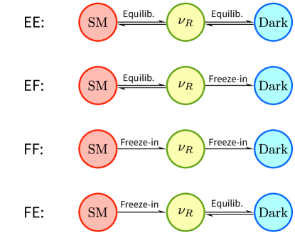
We aim at a comprehensive study of various possible scenarios arising from the framework of Eq. (2.1). Depending on the coupling and also on how RHNs interact with the SM, there are four possible cases we may encounter, as illustrated in Fig. 1 and elucidated as follows.
-
•
Equilibrium-Equilibrium (EE): both and the dark sector are in thermal equilibrium with the SM thermal bath. In this case, if is lighter than DM, then it is essentially in the standard WIMP paradigm. The DM abundance is determined by the moment when freezes out. If is heavier than DM, it becomes more complicated since is kinematically suppressed in the non-relativistic regime.
-
•
Equilibrium-Freeze-in (EF): is in thermal equilibrium with the SM whereas the dark sector is frozen-in from . In this case, the DM abundance is determined by the integrated production rates of and from . The production rates crucially depend on whether is kinematically allowed or not. In any case, the production process is always kinematically allowed at high temperatures.
-
•
Freeze-in-Freeze-in (FF): no thermal equilibrium is reached between and the SM thermal bath, or between the dark sector and . DM is produced via a two-step freeze-in mechanism.
-
•
Freeze-in-Equilibrium (FE): is frozen-in from the SM and keeps thermal equilibrium with the dark sector. In this case, the DM abundance depends on how many particles have been produced through the thermal history, if is heavier than and dominantly decays to and . If is lighter than , the DM abundance also relies on the freeze-out of .
2.3 Boltzmann equations
For a generic species , the number density is governed by the following Boltzmann equation:
| (2.4) |
where is the Hubble parameter and is the collision term including contributions of all processes that create or annihilate particles. For , , or in our framework, each collision term may receive contributions from several reaction processes:
| (2.5) | ||||
| (2.6) | ||||
| (2.7) |
Here the subscripts of the ’s on the right-hand side indicate the specific processes, except for which generically stands for unspecified processes connecting the SM and . In practice, not all the processes above have to be taken into account; some may be suppressed or kinematically forbidden.
For a generic two-to-two process, , the collision term is formulated as
| (2.8) |
with
| (2.9) |
where ; is the momentum distribution function of particle ; denotes the matrix element of the process (see Tab. 1); and denotes the delta function responsible for momentum conservation. The “” sign takes “” for bosons and “” for fermions.
For one-to-two or two-to-one processes, the collision terms are similar except that one of the initial or final particles in Eq. (2.9) is removed.
| Processes | Processes | ||
|---|---|---|---|
![[Uncaptioned image]](/html/2212.09109/assets/x2.png) |
light- approx. | ![[Uncaptioned image]](/html/2212.09109/assets/x3.png) |
heavy- approx. |
![[Uncaptioned image]](/html/2212.09109/assets/x4.png) |
light- approx. | ![[Uncaptioned image]](/html/2212.09109/assets/x5.png) |
light- approx. |
![[Uncaptioned image]](/html/2212.09109/assets/x6.png) |
light- approx. heavy- approx. | ![[Uncaptioned image]](/html/2212.09109/assets/x7.png) |
light- approx. heavy- approx. |
Since the SM thermal bath has much more degrees of freedom than the dark sector, the total energy density of the early universe is dominated by the SM content. The Hubble parameter is determined by
| (2.10) |
where and denote the SM energy density and temperature, denotes the energy density of the -- sector, and GeV. For convenience, we have defined where is the effective number of degrees of freedom in and . For the SM , we adopt the results in Figure 2.2 of Ref. Wallisch:2018rzj . For additional species that are produced via freeze-in and stay in the freeze-in regime, their energy densities are low. For additional species that undergo non-relativistic freeze-out, their contributions to are also suppressed at the moment of freeze-out. Therefore, only for Cases EF and EE with light , receives a sizable contribution from .
The SM entropy density, , depends on a slightly different effective number of degrees of freedom, . In most cases, we neglect the small difference and assume .
The total entropy of the SM thermal bath in a comoving volume is approximately conserved, i.e. where is the scale factor in the FRW metric. Using , we obtain
| (2.11) |
In the freeze-in regime, can be computed as follows. Using Eq. (2.11) together with Eq. (2.4) one gets which can be written as
| (2.12) |
where in the integral depends on the integration variable . If does not change significantly during the relevant epoch, the integral in Eq. (2.12) can be written in terms of :
| (2.13) |
where denotes the freeze-in value of , i.e. it denotes the value of at the point when the integrand peaks. Taking a decay process for example, it should be when the decaying particle becomes non-relativistic.
After freeze-in, the comoving number density of is conserved and would remain as a constant if scales as . However, due to many subsequent annihilation of SM species, actually scales as . Therefore, as the universe cools down, the variation of leads to the following correction to :
| (2.14) |
where denotes the freeze-in value of , similar to introduced above.
Let us finally comment on the use of the integrated Boltzmann equation (2.4) and the momentum distribution functions, denoted by for , , or . For later convenience, we also denote the momentum distribution function of in thermal equilibrium by . If is not in thermal equilibrium, can be very different from .
Strictly speaking, for non-thermal , one needs to solve the more fundamental Boltzmann equation for rather than the integrated one for but under certain circumstances the latter suffices for accurate calculations. For non-thermal species being produced (frozen-in) from a thermal sector, the back-reaction is negligible and those factors due to Fermi-Dirac or Bose-Einstein statistics [such as in Eq. (2.9)] are also negligible. So the collision term mainly depends on quantities of thermal species and hence can be well determined. When studying the connection between two thermal or almost thermal sectors (such as the freeze-out scenario), the integrated form could also be approximately used because the collision term can be written in terms of number densities.
For non-thermal species being produced from another non-thermal species, however, the spectral shape of the latter can significantly affect the result. In this case, one needs more elaborated treatments involving numerical techniques and analytical approximations, as we will elucidate in Sec. 3.1.2.
3 DM relic abundance
With the framework set up in Sec. 2, we now start to investigate the four generic cases proposed in Fig. 1. The goal is to derive generic formulae for the DM relic abundance and also the criteria for identifying the four cases. The results are summarized in Tab. 2.
| Cases | light limit () | heavy limit () | ||
|---|---|---|---|---|
| Valid range of | Valid range of | |||
| EE | Eq. (3.17) | Eq. (3.26) | ||
| EF | Eq. (3.4) or (3.7) | Eq. (3.20) | ||
| FF | Eq. (3.11) | Eq. (3.28) | ||
| FE | Eq. (3.17) | Eq. (3.28) | ||
The results crucially depend on whether is kinematically allowed () or not () because the collision term is much larger, roughly by a factor of , than and . For simplicity, we assume in the decay-allowed case, and in the decay-forbidden case. In what follows, they are referred to as the heavy and light limit, respectively. Increasing or decreasing to a level comparable to without crossing the threshold () would lead to qualitatively similar results, though the calculations would be much more complicated.
3.1 Light limit
In the light limit, i.e., , the analyses and results below are almost independent of , which in principle can vary freely from any scales well below down to zero. If sufficiently light, might contribute to and hence be constrained by the precision measurement of .
3.1.1 Case EF in the light limit
Let us start with a sufficiently small so that the dark sector is not thermalized, while the sector is in thermal equilibrium. This corresponds to the EF case in Fig. 1. The dark sector particles are produced from via and . The latter contributes indirectly to the production of via decay. Let us first concentrate on the process. The collision term is calculated in Appendix A and can be approximately written as
| (3.1) |
where is the modified Bessel functions of order . In the derivation of this result, we have assumed , , and the Boltzmann statistics.
Given the collision terms, the number densities of and can be computed by solving the Boltzmann equations which in the freeze-in regime have solutions of the integral forms in Eqs. (2.12) and (2.13). Substituting Eq. (3.1) into Eq. (2.13) and integrating it down to a temperature well below , we obtain the number density of after freeze-in. In addition, we also take the correction in Eq. (2.14) into account. The result reads:
| (3.2) |
Apart from the direct production of particles via , there is also an indirect production channel via followed by decay. The lifetime of is much shorter than the age of the universe if . Therefore, almost all particles produced in the early universe will eventually decay to and . Since both and are proportional to , the production rates of should be comparable to that of . Indeed, according to the calculation in Appendix A [see Eqs. (A.10) and (A.11)], the number density of after freeze-in assuming does not decay would be
| (3.3) |
Taking decay into account, each particle produces one particle via . Hence the number density of is increased by .
It is conventional to write the result in terms of where is the ratio of to the critical energy density and with the Hubble constant today. In terms of , the result reads (including the contribution of decay):
| (3.4) |
Note that, as mentioned below Eq. (2.10), in this case receives an addition contribution from light . So the value of should be the SM value at freeze-in plus , assuming a single flavor of .
Eq. (3.4) implies that to generate in the EF case, one needs for thermalized and . This is consistent with the result in Ref. Hufnagel:2021pso , see Fig. 3 therein.
The validity of the above analysis for the EF case is based on the assumption that is sufficiently small. In this regime, the back-reactions is negligible due to the low density of particles. Now let us increase , which will eventually lead to a high back-reaction rate comparable to the production rate. Then the equilibrium between and will be established, leading to . Substituting into Eq. (3.2) and solving it for , we obtain the following solution:
| (3.5) |
For , the freeze-in calculation is approximately valid. For , it becomes the EE case, which will be discussed in Sec. 3.1.3.
Finally we would like to comment on a potentially important contribution from the off-shell decay. Although is lighter than and , off-shell can be produced from SM particle scattering and then decay to and . This part of contribution depends on the coupling of to the SM. In particular, in the presence of a relatively strong -SM interaction, the effective thermal mass of might actually exceed so that the production rate of the forbidden channel can be considerably large. This is very similar to the plasmon decay () used to constrain neutrino magnetic moments Raffelt1996 ; Capozzi:2020cbu ; Li:2022dkc . A dedicated treatment requires taking finite-temperature effects into account consistently in both scattering and decay processes Li:2022rde ; Li:2023ewv , which will be studied in our future work.
Here we provide a straightforward estimate of this contribution assuming that the finite-temperature effects are negligible and that couples to a pair of SM particles with a different coupling . The collision term for two light SM particles scattering to produce and is
| (3.6) |
Comparing it to Eq. (3.1), one can see that this channel dominates when . For , the DM relic abundance is given by
| (3.7) |
For , one should use Eq. (3.4) instead.
3.1.2 Case FF in the light limit
In the FF case, is not in thermal equilibrium so the result depends on the specific form of the momentum distribution function of . For the FF case, we modify Eq. (3.1) as follows:
| (3.8) |
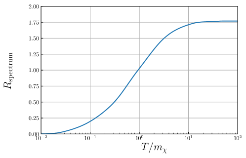
where is, by definition, to absorb the difference between FF and EF collisions terms for . Since , we expect to be around the same order of magnitude as . Hence we introduce a spectral distortion factor defined as
| (3.9) |
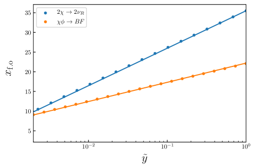
In the absence of spectral distortion (), we have . For light produced from heavy particle decay, the spectral shape of in the freeze-in regime can be computed analytically Heeck:2017xbu ; Decant:2021mhj —see also Appendix B for a brief review. With the analytical expression for , we can compute numerically111Here we have used the code available at https://github.com/xunjiexu/Thermal_Monte_Carlo., extract in Eq. (3.8), and then obtain the spectral distortion factor , which is presented in Fig. 2.
Using the numerical value of , we repeat the analysis in Sec. 3.1.1 and find that the non-thermal results in the following correction to the DM relic abundance in Eq. (3.4):
| (3.10) |
Therefore, for the FF case, the DM relic abundance abundance can be written as
| (3.11) |
Here we have assumed that is approximately a constant during the epoch of the second freeze-in of FF. This is a good approximation if the two freeze-in processes of FF occur at well separated temperature scales. If the two freeze-in temperatures are close to each other, then Eq. (3.11) is not valid but it can be used as a crude estimate. The exact result in this case can be obtained by numerical integration.
3.1.3 Cases EE and FE in the light limit
The EE and FE cases in Fig. 1 require that the dark sector keeps thermal equilibrium with . The criteria for such cases are just mentioned above.
In these two cases, we have at temperatures well above both masses. As the temperature falls below , a large amount of particles will annihilate to , leaving only a small portion of particles due to the well-known freeze-out mechanism. Since the freeze-out mechanism has been extensively studied, we refer to textbooks Kolb:1990vq ; Dodelson2003 and lectures Plehn:2017fdg ; Lisanti:2016jxe ; Lin:2019uvt for a full calculation starting from the Boltzmann equation. Here one can adapt the known result of the standard freeze-out calculation to our framework, with the key difference being that the -dark sector may have a different temperature compared to the SM one. The details are presented in Appendix C and the results are summarized below.
For convenience, we define two ratios
| (3.12) |
and denote their corresponding freeze-out values by and . In the EE case, we have . In the FE case, depends on the abundance of produced from the SM sector. The value of according to Appendix C is approximately given by
| (3.13) |
In the standard WIMP paradigm, typically varies around .
The relic abundance of DM is given by
| (3.14) |
where is the velocity-averaged cross section, widely used in the WIMP paradigm. It is related to the collision term by
| (3.15) |
and in the non-relativistic regime given by
| (3.16) |
Substituting Eq. (3.16) into Eq. (3.14), we obtain
| (3.17) |
Similar to the discussion below Eq. (3.4), in this case receives an addition contribution from light . So the value of should be the SM value at freeze-out plus , assuming a single flavor of .
Note that in the EE and FE cases, the influence of on the DM abundance should be small if because is small at the freeze-out temperature. Taking and for example, we get . Although the observed value of has been determined very precisely (), a 9% variation of can be easily absorbed into a small variation of , which is a rather free parameter in the model. So here we neglect the contribution of to the DM abundance.
A particularly interesting feature of the FE case is that due to the DM annihilation at a relatively late epoch, the abundance of might be substantially enhanced, causing observable changes to if are sufficiently light.
3.2 Heavy limit
In the heavy limit (), as well as its back-reaction is kinematically allowed. In the presence of , the energy conversion between the two sectors via such two-to-one or one–to-two processes is much more efficient than that via two-to-two processes considered in Sec. 3.1. Therefore, the contributions of and will be neglected in what follows.
3.2.1 Case EF in the heavy limit
Similar to the analysis in Sec. 3.1, we start with a sufficiently small so that the dark sector is not thermalized. On the other hand, the sector may or may not be in thermal equilibrium with the SM thermal bath, depending on the interaction of with the SM. Let us first consider that the -SM coupling is sufficiently large so that the sector has been thermalized. This leads to the EF case. The collision term for the dominant DM production process reads
| (3.18) |
Now substituting Eq. (3.18) into Eq. (2.13) and taking the correction in Eq. (2.14) into account, we obtain the values of and after freeze-in:
| (3.19) |
As we have assumed , cannot decay to and . However, this does not mean that would be stable. As long as the -SM coupling is not extremely suppressed, can eventually decay to and some SM final states with as an intermediate state. And the lifetime of is generally expected to be much shorter than the age of the universe. So for today’s , we should take . Consequently, today’s DM relic abundance is given by
| (3.20) |
Note that there is an interesting exception known as the SuperWIMP mechanism Covi:1999ty ; Feng:2003xh ; Feng:2003uy in which had been in thermal equilibrium but froze out before the freeze-in process started. Strictly speaking, this does not belong to the EF case because has already decoupled from the thermal bath when the majority of DM is being produced via . We will discuss this exception in Sec. 3.2.3.
Similar to Eq. (3.5), there is also an upper limit of for the validity of the freeze-in calculation. This is determined by equating to its equilibrium value. By solving it for , we obtain the equilibrium criterion:
| (3.21) |
For , the above calculation for the EF case is valid. Otherwise, it becomes the EE case, as we will discuss below.
3.2.2 Case EE in the heavy limit
For exceeding the limit in Eq. (3.21), and are in thermal equilibrium with the SM thermal bath, entering the EE case. As the universe cools down to a temperature below and , the energy and entropy stored in the - sector will be released via off-shell (virtual) to the SM thermal bath. The calculation for this scenario requires assumptions on the -SM interaction. To proceed, we assume that is coupled to a pair of SM particles ( and ) similar to Eq. (2.1) with a different coupling :
| (3.22) |
Here is a chiral fermion and a scalar boson, with masses well below . With the interaction in Eq. (3.22), the most efficient channel converting particles in the dark sector particles to SM species is co-annihilation—see e.g. Griest:1990kh ; Edsjo:1997bg ; Berlin:2017ife . Through the -channel tree-level process , each pair of and can be efficiently converted to a pair of and when the dark sector becomes non-relativistic. The process stops when and particles are too rare to meet each other, i.e., when . Hence similar to the standard WIMP freeze-out, there is also freeze-out in the co-annihilation scenario.
The co-annihilation collision term in the non-relativistic regime and in the small mass splitting limit reads:
| (3.23) |
Correspondingly, the velocity-averaged cross section is
| (3.24) |
3.2.3 Cases FF and FE in the heavy limit
In these two cases, after a certain amount of particles are produced via freeze-in, they will eventually decay to and particles, if we assume that is the dominant decay mode of . This is expected in the FE case because should be more tightly coupled to the dark sector than to the SM sector. As for the FF case, a considerably large part of the parameter space should meet the assumption. Hence for both cases under this assumption, the number density of is determined by the number of accumulated during the first freeze-in:
| (3.27) |
Here we have added a factor of to account for the contribution of decay—see the discussion below Eq. (3.19).
Assuming is produced via Eq. (3.22), the integral in Eq. (3.27) gives
| (3.28) |
Note that the result is independent of . Although can be used to tell whether it belongs to the FF or FE case, the difference between the two cases becomes unimportant as long as dominantly decays to and . The dominance can be guaranteed if which is plausible if one compares the benchmark value of in Eq. (3.28) to in Eq. (3.21).
As previously mentioned in Sec. 3.2.1, heavy could allow for the SuperWIMP mechanism Covi:1999ty ; Feng:2003xh ; Feng:2003uy in which DM is produced from frozen-out . This scenario is technically similar to the FF case because has decoupled from the SM thermal bath when it becomes responsible for DM production. Assuming that dominantly decays to the dark sector, the abundance of DM can be estimated from the number density of after the freeze-out. In the SuperWIMP mechanism, the dominance could be achieved by setting or . Under this assumption, the DM relic abundance is given by
| (3.29) |
Here we would like to compare the FF and FE cases in the heavy limit with the corresponding ones in the light limit. In the FF case with , the second freeze-in () stops when the kinetic energy drops below the mass of . In particular, after this freeze-in stops, a large amount of may still be present. In the FF case with , the second freeze-in can only be stopped by complete depletion of . Hence the production rate does not need to compete with the Hubble expansion, rendering unimportant as we have just mentioned.
As for the FE case, the -- coupled sector acquires a certain amount of energy and entropy injected from the SM thermal bath. The key difference between and is that the majority of this portion of energy and entropy will eventually be stored in the lightest species, which is (for ) or (for ).
Finally, we would like to comment on a potentially important two-to-two process in the heavy limit. For heavy , DM could be directly produced by the scattering of two SM particles, through an off-shell as the intermediate state, to and . At , this is the dominant channel for DM production. The collision term of such a process assuming Eq. (2.6) is proportional to , suppressed by in the heavy limit, whereas the production via on-shell decay is exponentially suppressed. Despite the dominance of the two-to-two process at , the overall contribution after integrating over is still subdominant compare to that of on-shell decay.
3.3 Discussions
The calculations presented above are all based on the assumption that the dark sector only interacts with the SM via . However, in this framework, the singlet scalar can be readily coupled to the SM Higgs via the Higgs portal. Assuming that the Higgs portal interaction is , to avoid a significant amount of dark sector particles being produced via the Higgs portal, the coupling needs to sufficiently small.
Here let us briefly estimate the production rate of via in the early universe. The matrix element for this process is simply an energy-independent constant, . For , we obtain the following collision term:
| (3.30) |
which is similar to the collision term. So it implies that for a sufficiently small , it should be in the freeze-in regime. Following the usual freeze-in calculation, we obtain that the abundance of (in the absence of decay) would be comparable to if . Therefore, we conclude that for well below , the Higgs portal interaction can be neglected.
4 Application: Type-I seesaw dark matter
In this section, we apply our framework to the type-I seesaw model, i.e., we take the type-I seesaw model and extend it by a pair of dark particles, and , with the interaction given by Eq. (2.1). Such an extension can accommodate an absolutely stable DM candidate and meanwhile still retain the virtue of being responsible for light neutrino masses via the type-I seesaw mechanism.
The type-I seesaw Lagrangian reads:
| (4.1) |
where is the SM Higgs doublet in the unitarity gauge, , and is a lepton doublet. After the electroweak symmetry breaking, the above Yukawa interaction gives rises to the Dirac mass term, with . Then at low energy scales, acquires an effective Majorana mass via the seesaw mechanism:
| (4.2) |
For simplicity, we ignore the flavor structure and regard , , and all as single-value quantities rather than matrices.
It is noteworthy that the type-I seesaw model itself in principle allows for one of the ’s to be a DM candidate in the keV regime—see e.g. the so-called MSM Asaka:2005pn ; Asaka:2005an . However, since the simplest scenario where the keV sterile neutrino DM is produced by the Dodelson–Widrow mechanism Dodelson:1993je has been excluded by -ray and Lyman- observations, we do not consider the possibility that servers as a DM candidate in this work.
Given the approximately known scale of , we make use of the seesaw mass relation (4.2) to determine the Yukawa coupling:
| (4.3) | ||||
| (4.4) |
where we have assumed eV.
The seesaw mechanism also leads to the active-sterile neutrino mixing with the mixing angle given by
| (4.5) |
Below we will show that and determined by the type-I seesaw relation are sufficiently large to thermalize . Hence the type-I seesaw DM is always in the EE or EF case.
4.1 Production rates of via Yukawa and gauge interactions
4.1.1 Above the electroweak scale
For well above the electroweak scale, the dominant process for production is . The collision term is
| (4.6) |
Using , we can estimate [similar to the derivation of Eq. (3.21)] the criterion for reaching thermal equilibrium:
| (4.7) |
which is always satisfied according to Eq. (4.3). Therefore, must have been in thermal equilibrium if is determined by the seesaw relation and is well above the electroweak scale.
4.1.2 Below the electroweak scale
For well below the electroweak scale, is kinematically forbidden but is allowed. The collision term is similar:
| (4.8) |
where GeV is the Higgs mass.
In addition to the Higgs decay, can also be produced via and decays. One can compute the decay widths either in the mass-eigenstate basis or in the chiral basis. The results from the two different approaches are the same. Taking decay as an example, in the mass-eigenstate basis, it is straightforward to obtain , though strictly speaking one should replace and with their respective dominant mass eigenstates. In the chiral basis, one treats the Dirac mass term as a perturbative term so that the Feynman diagram contains a mass insertion proportional to and an intermediate propagator proportional to . The propagator effectively contributes a factor of after imposing the on-shell condition of . So the diagram is suppressed by a factor of , and is suppressed by . Therefore, in either way, one obtains
| (4.9) | ||||
| (4.10) |
where is the SM gauge coupling and is the Weinberg angle. Compared to Eq. (4.8), the rates of production via and decays are enhanced by . This conclusion is consistent with the previous calculation in Ref. Coy:2021sse .
Note that below the electroweak scale can also be produced via neutrino oscillations which, as we will show below, are much more efficient than the decay processes.
4.2 Production rates of via oscillations
Neutrino oscillations in the early universe have been extensively studied as they play a key role in sterile neutrino DM—see Dasgupta:2021ies ; Kusenko:2009up ; Abazajian:2017tcc ; Adhikari:2016bei for recent reviews. In the non-resonant production (NRP) regime with negligible lepton asymmetries, the production rate of reads lesgourgues_book ; Abazajian:2001nj ; Gelmini:2019wfp :
| (4.11) |
with
| (4.12) | ||||
| (4.13) |
where and is the effective mixing angle which is related to but different from due to the thermal MSW potential, . Unlike the conventional MSW potential proportional to , in the cosmological thermal plasma is proportional to . This is because the contributions of particles and anti-particles in the background cancel out at the leading order. According to Eq. (4.13), at low temperatures (), we have while at high temperatures would be suppressed by .
By comparing with given in Eq. (4.11) to Eq. (4.8), we obtain
| (4.14) |
where as a crude approximation we have taken for and only integrated below the corresponding temperature. The actual integral in the denominator is larger, leading to a more suppressed ratio. Eq. (4.14) implies that the production of via neutrino oscillations is much more efficient than that from Higgs decay, as long as is below the electroweak scale.
To check whether neutrino oscillations could bring into thermal equilibrium, we compare with the Hubble parameter:
| (4.15) |
where the ratio is estimated at the temperature when peaks, i.e., when in the denominator of Eq. (4.13) is equal to .
Eq. (4.15) implies that the production rate of via oscillation is sufficiently high to render thermal, provided that its mass is below the electroweak scale and the mixing angle is determined by the seesaw relation. This conclusion is consistent with Ref. Dolgov:2003sg which obtained as the condition for to reach equilibrium—see Eqs. (38) and (39) therein.
4.3 Benchmarks
As we have shown in Sec. 4.1 and Sec. 4.2, the production rate of in the early universe is sufficiently high for to reach thermal equilibrium, provided that the interaction of with the SM is determined by the type-I seesaw mass relation222This is only true when we neglect the flavor structure, which in principle could accommodate three rather hierarchical ’s. In fact, one could have two ’s responsible for the observed light neutrino masses and one with much more suppressed and than those given in Eqs. (4.4) and (4.5) so as to circumvent the restriction of the seesaw mass relation—see, e.g., Refs. Coy:2021sse ; Coy:2022xfj .. Therefore, the type-I seesaw DM is either in the EE or EF case, depending on the dark sector coupling introduced in Eq. (2.1).
Now let us consider some specific benchmarks for the type-I seesaw DM:
| Benchmark L1: | |||
| Benchmark L2: | |||
| Benchmark H1: | |||
| Benchmark H2: |
Here L/H indicates that is much lighter/heavier than . Two of the benchmarks are at TeV scales and the other two at GeV scales. We set a small but sizable mass splitting between and so that eventually all particles produced in the early universe decay to and other particles.
According to Tab. 2, Benchmarks L1 and L2 would be in the EE case if or in the EF case if . For Benchmarks H1 and H2, the criterion is similar except that is changed to .
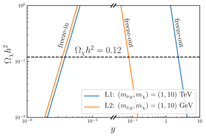
Let us first concentrate on Benchmarks L1 and L2, for which the DM candidate is produced via . When is small (), this is a freeze-in process and, according to Tab. 2, we take Eq. (3.4) with to compute . The results are presented in the left panel of Fig. 3 as the increasing lines (labeled “freeze-in”) which go across at
| (4.16) |
The small difference is caused by the value of at freeze-in [see in Eq. (3.4)] which is evaluated at . For L1, the freeze-in temperature is well above the electroweak scale, hence . At GeV (the case of L2), falls to Wallisch:2018rzj .
If we increase to a sufficiently large value, it will enter the EE regime. The DM candidate keeps in thermal equilibrium via until it becomes non-relativistic and freezes out from the thermal bath. According to Tab. 2, the relic abundance is determined by Eq. (3.17), corresponding to the decreasing lines (labeled “freeze-out”) in the left panel of Fig. 3. The two lines go across at
| (4.17) |
Note that in the EE regime, larger implies larger in order to account for the correct DM relic abundance. If one sets to higher values TeV, then would exceed the unitarity bound (). This is known as the Griest-Kamionkowski bound, which dictates that thermal freeze-out DM should be lighter than TeV Griest:1989wd , otherwise the annihilation cross section would be too large and violate the unitarity bound.
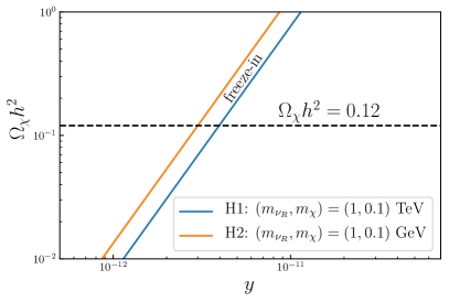
Next, let us turn to Benchmarks H1 and H2. Due to , the DM candidate is directly produced via decay, . Therefore, the critical value of separating the EE and EF cases is much smaller than that for L1 and L2. For , Benchmarks H1 and H2 are in the EF regime. Hence we take Eq. (3.20) to compute . The results are presented in the right panel of Fig. 3 as the increasing lines which go across at
| (4.18) |
For larger , in principle it could enter the EE regime. However, it turns that for Benchmarks H1 and H2 there are no freeze-out solutions if the neutrino-Higgs coupling is determined by the seesaw mass relation. This is because due to its heavy masses in these two benchmarks cannot be the final states of DM (co-)annihilation processes. The dark sector particles and have to annihilate or co-annihilate to lighter SM species. Possible processes could be mediated by an off-shell , or via box diagrams, with and as intermediate states, etc. If is not kinematically suppressed, it is the dominant process for DM freeze-out. Using Eq. (3.26) with determined by Eq. (4.4) and neglecting the Higgs mass, one would obtain for Benchmark H1. This obviously violates the unitarity bound. In other words, if is limited within the unitarity bound (), then the cross section of the dominant freeze-out process would be too small to deplete the overproduced DM. For Benchmark H2 where is well below the electroweak scale, is kinematically suppressed. One would have to consider other processes that are further suppressed by additional vertices in the diagrams.
There is, however, an interesting scenario that could potentially allow freeze-out solutions for heavier than . According to Eq. (3.26) where is roughly [neglecting all quantities] proportional to , if is sufficiently light (e.g., keV), then could be suppressed by , possibly leading to a freeze-out solution. Using Eqs. (3.26) and (3.25) with and , we find that the freeze-out solution is at keV. By varying and one can obtain different values, but the mass scale cannot be much higher than the keV scale. Despite the existence of such freeze-out solutions, this scenario is ruled out by BBN observations due to additional thermal species at the MeV scale. If we only consider that these particles are well above the MeV scale, and if the magnitude of is subject to the seesaw constraint, then the type-I seesaw DM with heavier than cannot have a freeze-out solution.
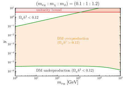

In Fig. 4, we show the parameter space of the type-I seesaw DM model assuming two different mass ratios, one with and the other with . As previously discussed, the heavy scenario does not allow for freeze-out solutions. So the blue curve in the right panel of Fig. 4 is a freeze-in solution for . The value of of this solution varies in a limited range from to due to the variation of . In the left panel, the variation of the freeze-in solution due to is insignificant but it bends down significantly at GeV because the -channel contribution in Eq. (3.7) becomes dominant. In addition, there is also a freeze-out solution (the top green line) which would exceed the unitarity bound for TeV.
5 Observational consequences
DM produced via the RHN portal is difficult to probe via direct detection experiments because it does not directly interact with normal matter consisting of electrons and quarks. Nevertheless, we would like to point out an interesting process, , with and as intermediate states. This process might be possible if the active-sterile neutrino mixing is not too small. The major concern is that the non-relativistic might not have sufficient energy to cause an observable electron recoil, unless has been boosted.
Regarding indirect detection, the annihilation process produces two RHNs which may subsequently decay to stable particles (, , , etc.) in the SM, as has recently been studied comprehensively in Ref. Morrison:2022zwk . Alternatively, can be more straightforwardly produced from annihilation at the one-loop level with , , and appearing in a box diagram. We make a crude estimation and find that that the annihilation cross section is too small to to be relevant to the current indirect detection experiments. In addition to annihilation, one might consider the decay as a source of indirect detection signals. As estimated below Eq. (3.2), if is light, is possible but the coupling or the mass splitting has to be extremely suppressed in order to render long-lived at a cosmological time scale. If is heavy, may decay to and, via an off-shell , to some SM states. In this scenario, the lifetime of can be substantially longer but whether there is viable parameter space for observable indirect detection signals remains an open question.
Perhaps the most interesting observational consequence is the cosmological effective number of relativistic species, . If RHNs are sufficiently light, they may contribute to . As is well known, neutrinos can be Dirac particles and this possibility motivates extensive studies on the potential contribution to Abazajian:2019oqj ; Luo:2020sho ; Borah:2020boy ; Adshead:2020ekg ; Luo:2020fdt . In our framework, a particularly noteworthy scenario is the FE case with very light . Through the freeze-in from the SM to , a considerably large amount of energy and entropy can be transferred to the dark sector, which after undergoing freeze-out at a relatively late epoch will release almost all the entropy stored in the dark sector to . In this scenario, the contribution to can be very significant without overproducing DM. In contrast, DM frozen-in from or more directly from usually cannot change significantly Hufnagel:2021pso ; Li:2021okx because the amount of energy transferred to DM is limited by , corresponding to which is much lower than the neutrino number density. The potentially significant contribution to in the FE case calls for a more dedicated study in light of current and upcoming precision measurements of .
6 Conclusion
In this paper we have presented a comprehensive investigation of a generic framework in which DM is produced from the RHN portal. As formulated in Eq. (2.1), our framework assumes that a RHN () is coupled to a dark fermion (, which serves as DM with absolute stability) and a dark scalar (). Since the analyses crucially depend on whether the equilibrium between and the SM, and between the dark sector and , can be established, we propose four basic cases, namely EE, EF, FF, and FE, as illustrated in Fig. 1. Our results of the DM relic density and the criteria for identifying the four cases have been summarized in Tab. 2. Note that the results also depend on whether is heavy or light compared the mass scale of the dark sector, because the dominant production processes are decay and annihilation for heavy and light , respectively.
As a simple application, we considered the type-I seesaw model extended by the dark sector in our framework. We found that when the neutrino-Higgs Yukawa coupling is determined by the seesaw mass relation, the thermal history of the dark sector can only be in the EE or EF case. For light , both have viable solutions accounting for the correct DM relic abundance, while for heavy , only EF is viable—see Fig. 3.
Finally, we discussed a few observational consequences in this framework. Although it seems difficult to cause observable signals in direct detection experiments, the RHN-portal DM may have important implications for indirect detection and future precision measurements of .
Acknowledgements.
We thank Rupert Coy for useful discussions. This work is supported in part by the National Natural Science Foundation of China under grant No. 12141501.Appendix A Collision terms
The analytical calculations presented below assume the Maxwell-Boltzmann statistics, which implies not only that the Maxwell-Boltzmann distribution is used for bosonic and fermionic species, but also that in Eq. (2.9) are neglected. With this assumption, the number density can be computed as follows:
| (A.1) |
The collision terms for two-to-two, two-to-one, and one-to-two processes take the following forms:
| (A.2) | ||||
| (A.3) | ||||
| (A.4) |
The collision terms computed assuming the Maxwell-Boltzmann statistics typically deviate from the exact values by —see e.g. Tab. III in Ref. Luo:2020sho .
A.1 Two-to-two collision terms
Let us first consider a two-to-two process, generically denoted by .
Assuming and , the collision term can be computed analytically Gondolo:1990dk :
| (A.5) |
where is the total cross section of this process.
For , the cross section reads
| (A.6) |
where . Substituting Eq. (A.6) into Eq. (A.5), we obtain the result in Eq. (3.1). In particular, has the following high- and low-temperature limits (assuming in thermal equilibrium):
| (A.7) | ||||
| (A.8) |
For , the cross section reads
| (A.9) |
where . Substituting Eq. (A.9) into Eq. (A.5), we find that the integral of can only be calculated numerically but to a good approximation ( within ) it can be approximated as
| (A.10) |
where and are obtained via fitting. When the collision term is used in Eq. (2.13), we are mainly concerned with the integral . Numerically performing the integral, we find
| (A.11) |
which implies that with the same coupling and the small mass splitting limit (), the integrated production rate of is almost twice as large as that of .
For the co-annihilation process appeared in Sec. 3.2.2, we only consider cases with approximately equal masses of and . In addition, the process is only important at so we assume that is sufficiently heavy in our calculation. Under these assumptions, the cross section is given by
| (A.12) |
Substituting Eq. (A.12) into Eq. (A.5), we obtain the corresponding collision term. For a general value of , there is no simple expression for the result. Technically one can express the integral in terms of the Meijer G-function, but the expression is not useful in practice. We are only interested in the approximate result at , for which we have
| (A.13) |
A.2 Two-to-one or one-to-two collision terms
For and in Eqs. (A.3) and (A.4), we assume the initial and final state masses are negligible, respectively. Then we adopt the results from Appendix A of Ref. Luo:2020fdt and obtain
| (A.14) | ||||
| (A.15) |
It is worth mentioning that has the following high and low temperature limits:
| (A.16) | ||||
| (A.17) |
For , the limits are the same, except that is replaced by .
When dealing with the Boltzmann equation of a momentum distribution function [see Eq. (B.1)], one needs the following collision terms:
| (A.18) | ||||
| (A.19) |
where in or denotes the particle of which the distribution is to be computed.
Let us first compute Eq. (A.19), with the same assumptions as aforementioned. Integrating out , we obtain
| (A.20) |
where . One can further integrate out together with the function, provided that the argument in the function can reach zero when scans from to . It is straightforward to find out that this requires
| (A.21) |
Integrating out , we obtain
| (A.22) |
where arsing from . Finally, integrating out with , we obtain
| (A.23) |
One can check that reproduces the result in Eq. (A.15).
As for , the calculation is similar except that has both upper and lower bounds, , and the result is given as follows:
| (A.24) |
Again, one can check that reproduces the result in Eq. (A.14).
Appendix B Calculation of the freeze-in momentum distribution
The momentum distribution function, , is governed by the following Boltzmann equation:
| (B.1) |
where is the collision term for . In the freeze-in regime where the back-reaction is negligible, Eq. (B.1) can be written as an integral of . Below we show the details.
First, we introduce a transformation of variables from to where is the scale factor () and . Then the Jacobian matrix of this transformation reads
| (B.2) |
Next, we express Eq. (B.1) in terms of . As we will adopt as new variables, we define
| (B.3) |
and write
| (B.4) |
The zero entry in above allows us to write the left-hand side of Eq. (B.1) as a total derivative:
| (B.5) |
Replacing , we obtain
| (B.6) |
For a given collision term, one can use Eq. (B.6) to compute the momentum distribution function . For example, taking the collision term in Eq. (A.23), we obtain
| (B.7) |
where . In the limit of , the function reduces to unity and Eq. (B.7) reduces to
| (B.8) |
From Eq. (B.8), one can readily obtain the average value of , , which is lower than the well-known values for Maxwell-Boltzmann, Fermi-Dirac, and Bose-Einstein distributions, respectively.
For two-to-two processes, the integral in Eq. (B.6) generally cannot be analytically integrated but the numerical evaluation is straightforward.
Appendix C Calculation of the secluded freeze-out
In this appendix, we derive Eq. (3.14) for the secluded freeze-out scenario by revisiting the calculation for the standard freeze-out mechanism, with some steps modified in order to take into account that the dark sector has a different temperature as the SM sector.
Let us first inspect the freeze-out temperature, which is determined by
| (C.1) |
where approximately depends on while depends on the dark sector temperature . Before freeze-out, in the non-relativistic regime is given by
| (C.2) |
where has been defined in Eq. (3.12).
The freeze-out value of , denoted by , is determined by substituting Eq. (C.2) and Eq. (2.10) into Eq. (C.1):
| (C.3) |
which can be solved numerically to determined .
For the DM annihilation process, , is given by Eq. (3.15):
| (C.4) |
Using Eq. (C.4), we find that the solution of in Eq. (C.3) can be approximately fitted by
| (C.5) |
For the DM co-annihilation process, , we have with given by Eq. (A.13). The approximate solution reads:
| (C.6) |
In Fig. 5, we show how well the above approximate expressions can fit the exact results. In the figure, denotes the quantities in the square brackets of Eqs. (C.5) and (C.6).
Once is obtained from solving Eq. (C.3), the number density at the moment of freeze-out can be computed by
| (C.7) |
After freeze-out, the comoving number density is conserved while in the SM sector, many species will eventually annihilate and inject their energy into lighter species. Nevertheless, the SM comoving entropy density is conserved. Hence the ratio after freeze-out is a constant:
| (C.8) |
Using Eqs. (C.8), (C.7), (2.10), and , we obtain
| (C.9) |
Eq. (C.9) remains valid even in relatively late eras dominated by matter or by vacuum energy, provided that in these eras are interpreted as the entropy density of radiation (photons and neutrinos) and in Eq. (C.9) is interpreted as the photon temperature. Although the universe is dominated by non-radiation content in these eras, the comoving entropy of photons and neutrinos is conserved. Taking and K, we obtain from Eq. (C.9) today’s energy density of DM:
| (C.10) |
It is conventional to write the result in terms of which is defined by
| (C.11) |
where is the Hubble constant today and is the critical energy density. Note that is independent of (or ) so that it is not affected by the long-standing Hubble tension problem—see DiValentino:2021izs ; Efstathiou:2021ocp ; Schoneberg:2021qvd for latest reviews. Combining Eqs. (C.10) and (C.11), we obtain
| (C.12) |
References
- (1) P. Minkowski, at a Rate of One Out of Muon Decays?, Phys. Lett. B67 (1977) 421–428.
- (2) T. Yanagida, Proceedings of the Workshop on the Unified Theory and the Baryon Number in the Universe, KEK Report 79-18 (1979) 95.
- (3) M. Gell-Mann, P. Ramond, and R. Slansky, Complex Spinors and Unified Theories, Conf. Proc. C790927 (1979) 315–321, [1306.4669].
- (4) S. Glashow, The future of elementary particle physics, NATO Adv, Study Inst. Ser. B Phys 59 (1979) 687.
- (5) R. Mohapatra and G. Senjanovic, Neutrino mass and spontaneous parity nonconservation, Phys. Rev. Lett. 44 (1980), no. 14 912–915.
- (6) M. Fukugita and T. Yanagida, Baryogenesis Without Grand Unification, Phys. Lett. B 174 (1986) 45–47.
- (7) S. Davidson, E. Nardi, and Y. Nir, Leptogenesis, Phys. Rept. 466 (2008) 105–177, [0802.2962].
- (8) G. Bertone, D. Hooper, and J. Silk, Particle dark matter: Evidence, candidates and constraints, Phys. Rept. 405 (2005) 279–390, [hep-ph/0404175].
- (9) B. Dasgupta and J. Kopp, Sterile neutrinos, Phys. Rept. 928 (2021) 1–63, [2106.05913].
- (10) A. Kusenko, Sterile neutrinos: The dark side of the light fermions, Phys. Rept. 481 (2009) 1–28, [0906.2968].
- (11) K. N. Abazajian, Sterile neutrinos in cosmology, Phys. Rept. 711-712 (2017) 1–28, [1705.01837].
- (12) M. Drewes et al., A White Paper on keV Sterile Neutrino Dark Matter, JCAP 01 (2017) 025, [1602.04816].
- (13) S. Dodelson and L. M. Widrow, Sterile-neutrinos as dark matter, Phys. Rev. Lett. 72 (1994) 17–20, [hep-ph/9303287].
- (14) X.-D. Shi and G. M. Fuller, A new dark matter candidate: Nonthermal sterile neutrinos, Phys. Rev. Lett. 82 (1999) 2832–2835, [astro-ph/9810076].
- (15) J. Baur, N. Palanque-Delabrouille, C. Yeche, A. Boyarsky, O. Ruchayskiy, E. Armengaud, and J. Lesgourgues, Constraints from ly- forests on non-thermal dark matter including resonantly-produced sterile neutrinos, JCAP 12 (2017) 013, [1706.03118].
- (16) V. Iršič et al., New Constraints on the free-streaming of warm dark matter from intermediate and small scale Lyman- forest data, Phys. Rev. D 96 (2017), no. 2 023522, [1702.01764].
- (17) N. Palanque-Delabrouille, C. Yèche, N. Schöneberg, J. Lesgourgues, M. Walther, S. Chabanier, and E. Armengaud, Hints, neutrino bounds and WDM constraints from SDSS DR14 Lyman- and Planck full-survey data, JCAP 04 (2020) 038, [1911.09073].
- (18) A. Garzilli, O. Ruchayskiy, A. Magalich, and A. Boyarsky, How warm is too warm? Towards robust Lyman- forest bounds on warm dark matter, 1912.09397.
- (19) M. Pospelov, A. Ritz, and M. B. Voloshin, Secluded WIMP Dark Matter, Phys. Lett. B 662 (2008) 53–61, [0711.4866].
- (20) A. Falkowski, J. Juknevich, and J. Shelton, Dark matter through the neutrino portal, 0908.1790.
- (21) V. González-Macías, J. I. Illana, and J. Wudka, A realistic model for Dark Matter interactions in the neutrino portal paradigm, JHEP 05 (2016) 171, [1601.05051].
- (22) M. Escudero, N. Rius, and V. Sanz, Sterile Neutrino portal to Dark Matter II: Exact Dark symmetry, Eur. Phys. J. C 77 (2017), no. 6 397, [1607.02373].
- (23) Y.-L. Tang and S.-h. Zhu, Dark matter relic abundance and light sterile neutrinos, JHEP 01 (2017) 025, [1609.07841].
- (24) B. Batell, T. Han, and B. Shams Es Haghi, Indirect Detection of Neutrino Portal Dark Matter, Phys. Rev. D 97 (2018), no. 9 095020, [1704.08708].
- (25) P. Bandyopadhyay, E. J. Chun, R. Mandal, and F. S. Queiroz, Scrutinizing Right-Handed Neutrino Portal Dark Matter With Yukawa Effect, Phys. Lett. B 788 (2019) 530–534, [1807.05122].
- (26) M. Becker, Dark Matter from Freeze-In via the Neutrino Portal, Eur. Phys. J. C 79 (2019), no. 7 611, [1806.08579].
- (27) M. Chianese and S. F. King, The dark side of the littlest seesaw: freeze-in, the two right-handed neutrino portal and leptogenesis-friendly fimpzillas, JCAP 09 (2018) 027, [1806.10606].
- (28) M. G. Folgado, G. A. Gómez-Vargas, N. Rius, and R. Ruiz De Austri, Probing the sterile neutrino portal to Dark Matter with rays, JCAP 08 (2018) 002, [1803.08934].
- (29) M. Chianese, B. Fu, and S. F. King, Minimal Seesaw extension for Neutrino Mass and Mixing, Leptogenesis and Dark Matter: FIMPzillas through the Right-Handed Neutrino Portal, JCAP 03 (2020) 030, [1910.12916].
- (30) E. Hall, T. Konstandin, R. McGehee, and H. Murayama, Asymmetric Matters from a Dark First-Order Phase Transition, 1911.12342.
- (31) M. Blennow, E. Fernandez-Martinez, A. Olivares-Del Campo, S. Pascoli, S. Rosauro-Alcaraz, and A. V. Titov, Neutrino Portals to Dark Matter, Eur. Phys. J. C 79 (2019), no. 7 555, [1903.00006].
- (32) P. Bandyopadhyay, E. J. Chun, and R. Mandal, Feeble neutrino portal dark matter at neutrino detectors, JCAP 08 (2020) 019, [2005.13933].
- (33) E. Hall, R. McGehee, H. Murayama, and B. Suter, Asymmetric dark matter may not be light, Phys. Rev. D 106 (2022), no. 7 075008, [2107.03398].
- (34) M. Chianese, B. Fu, and S. F. King, Dark Matter in the Type Ib Seesaw Model, JHEP 05 (2021) 129, [2102.07780].
- (35) A. Biswas, D. Borah, and D. Nanda, Light Dirac neutrino portal dark matter with observable Neff, JCAP 10 (2021) 002, [2103.05648].
- (36) R. Coy, A. Gupta, and T. Hambye, Seesaw neutrino determination of the dark matter relic density, Phys. Rev. D 104 (2021), no. 8 083024, [2104.00042].
- (37) R. Coy and A. Gupta, A closer look at the seesaw-dark matter correspondence, 2211.05091.
- (38) B. Barman, P. S. Bhupal Dev, and A. Ghoshal, Probing Freeze-in Dark Matter via Heavy Neutrino Portal, 2210.07739.
- (39) L. Coito, C. Faubel, J. Herrero-García, A. Santamaria, and A. Titov, Sterile neutrino portals to Majorana dark matter: effective operators and UV completions, JHEP 08 (2022) 085, [2203.01946].
- (40) B. Wallisch, Cosmological Probes of Light Relics. PhD thesis, Cambridge U., 2018. 1810.02800.
- (41) M. Hufnagel and X.-J. Xu, Dark matter produced from neutrinos, JCAP 01 (2022), no. 01 043, [2110.09883].
- (42) G. G. Raffelt, Stars as laboratories for fundamental physics: The astrophysics of neutrinos, axions, and other weakly interacting particles. University of Chicago Press, 1996.
- (43) F. Capozzi and G. Raffelt, Axion and neutrino bounds improved with new calibrations of the tip of the red-giant branch using geometric distance determinations, Phys. Rev. D 102 (2020), no. 8 083007, [2007.03694].
- (44) S.-P. Li and X.-J. Xu, Neutrino Magnetic Moments Meet Precision Measurements, JHEP 02 (2023) 085, [2211.04669].
- (45) S.-P. Li, Strong scattering from decay for dark matter freeze-in, 2211.16802.
- (46) S.-P. Li, Dark matter freeze-in via a light thermal fermion mediator, 2301.02835.
- (47) J. Heeck and D. Teresi, Cold keV dark matter from decays and scatterings, Phys. Rev. D 96 (2017), no. 3 035018, [1706.09909].
- (48) Q. Decant, J. Heisig, D. C. Hooper, and L. Lopez-Honorez, Lyman- constraints on freeze-in and superWIMPs, JCAP 03 (2022), no. 03 041, [2111.09321].
- (49) E. W. Kolb and M. S. Turner, The Early Universe, Front. Phys. 69 (1990) 1–547.
- (50) D. Scott, Modern Cosmology. Academic Press, 2003.
- (51) M. Bauer and T. Plehn, Yet Another Introduction to Dark Matter: The Particle Physics Approach, vol. 959 of Lecture Notes in Physics. Springer, 2019.
- (52) M. Lisanti, Lectures on Dark Matter Physics, in Theoretical Advanced Study Institute in Elementary Particle Physics: New Frontiers in Fields and Strings, pp. 399–446, 2017. 1603.03797.
- (53) T. Lin, Dark matter models and direct detection, PoS 333 (2019) 009, [1904.07915].
- (54) L. Covi, J. E. Kim, and L. Roszkowski, Axinos as cold dark matter, Phys. Rev. Lett. 82 (1999) 4180–4183, [hep-ph/9905212].
- (55) J. L. Feng, A. Rajaraman, and F. Takayama, Superweakly interacting massive particles, Phys. Rev. Lett. 91 (2003) 011302, [hep-ph/0302215].
- (56) J. L. Feng, A. Rajaraman, and F. Takayama, SuperWIMP dark matter signals from the early universe, Phys. Rev. D 68 (2003) 063504, [hep-ph/0306024].
- (57) K. Griest and D. Seckel, Three exceptions in the calculation of relic abundances, Phys. Rev. D 43 (1991) 3191–3203.
- (58) J. Edsjo and P. Gondolo, Neutralino relic density including coannihilations, Phys. Rev. D 56 (1997) 1879–1894, [hep-ph/9704361].
- (59) A. Berlin, WIMPs with GUTs: Dark Matter Coannihilation with a Lighter Species, Phys. Rev. Lett. 119 (2017) 121801, [1704.08256].
- (60) T. Asaka and M. Shaposhnikov, The MSM, dark matter and baryon asymmetry of the universe, Phys. Lett. B 620 (2005) 17–26, [hep-ph/0505013].
- (61) T. Asaka, S. Blanchet, and M. Shaposhnikov, The MSM, dark matter and neutrino masses, Phys. Lett. B631 (2005) 151–156, [hep-ph/0503065].
- (62) J. Lesgourgues, G. Mangano, G. Miele, and S. Pastor, Neutrino Cosmology. Cambridge University Press, 2013.
- (63) K. Abazajian, G. M. Fuller, and M. Patel, Sterile neutrino hot, warm, and cold dark matter, Phys. Rev. D 64 (2001) 023501, [astro-ph/0101524].
- (64) G. B. Gelmini, P. Lu, and V. Takhistov, Cosmological Dependence of Non-resonantly Produced Sterile Neutrinos, JCAP 12 (2019) 047, [1909.13328].
- (65) A. D. Dolgov and F. L. Villante, BBN bounds on active sterile neutrino mixing, Nucl. Phys. B 679 (2004) 261–298, [hep-ph/0308083].
- (66) K. Griest and M. Kamionkowski, Unitarity Limits on the Mass and Radius of Dark Matter Particles, Phys. Rev. Lett. 64 (1990) 615.
- (67) L. Morrison, S. Profumo, and B. Shakya, Sterile neutrinos from dark matter: A nightmare?, 2211.05996.
- (68) K. N. Abazajian and J. Heeck, Observing Dirac neutrinos in the cosmic microwave background, Phys. Rev. D 100 (2019) 075027, [1908.03286].
- (69) X. Luo, W. Rodejohann, and X.-J. Xu, Dirac neutrinos and , JCAP 06 (2020) 058, [2005.01629].
- (70) D. Borah, A. Dasgupta, C. Majumdar, and D. Nanda, Observing left-right symmetry in the cosmic microwave background, Phys. Rev. D 102 (2020), no. 3 035025, [2005.02343].
- (71) P. Adshead, Y. Cui, A. J. Long, and M. Shamma, Unraveling the Dirac neutrino with cosmological and terrestrial detectors, Phys. Lett. B 823 (2021) 136736, [2009.07852].
- (72) X. Luo, W. Rodejohann, and X.-J. Xu, Dirac neutrinos and Neff. Part II. The freeze-in case, JCAP 03 (2021) 082, [2011.13059].
- (73) S.-P. Li, X.-Q. Li, X.-S. Yan, and Y.-D. Yang, Simple estimate of BBN sensitivity to light freeze-in dark matter, Phys. Rev. D 104 (2021), no. 11 115007, [2106.07122].
- (74) P. Gondolo and G. Gelmini, Cosmic abundances of stable particles: Improved analysis, Nucl. Phys. B 360 (1991) 145–179.
- (75) E. Di Valentino, O. Mena, S. Pan, L. Visinelli, W. Yang, A. Melchiorri, D. F. Mota, A. G. Riess, and J. Silk, In the realm of the Hubble tension—a review of solutions, Class. Quant. Grav. 38 (2021), no. 15 153001, [2103.01183].
- (76) G. Efstathiou, To H0 or not to H0?, Mon. Not. Roy. Astron. Soc. 505 (2021), no. 3 3866–3872, [2103.08723].
- (77) N. Schöneberg, G. Franco Abellán, A. Pérez Sánchez, S. J. Witte, V. Poulin, and J. Lesgourgues, The Olympics: A fair ranking of proposed models, Phys. Rept. 984 (2022) 1–55, [2107.10291].