A Degree Based Approximation of an SIR Model with Contact Tracing and Isolation

Abstract

In this paper we study a susceptible infectious recovered (SIR) model with asymptomatic patients, contact tracing and isolation on a configuration network. Using degree based approximation, we derive a system of differential equations for this model. This system can not be solved analytically. We present an early-time analysis for the model. The early-time analysis produces an epidemic threshold. On one side of the threshold, the disease dies out quickly. On the other side, a significant fraction of population are infected. The threshold only depends on the parameters of the disease, the mean access degree of the network, and the fraction of asymptomatic patients. The threshold does not depend on the parameter of contact tracing and isolation policy. We present an approximate analysis which greatly reduces computational complexity. The nonlinear system derived from the approximation is not almost linear. We present a stability analysis for this system. We simulate the SIR model with contact tracing and isolation on five real-world networks. Simulation results show that contact tracing and isolation are useful to contain epidemics.

1 Introduction

In the early stage of an outbreak when there are not many infected individuals, contact tracing, quarantine and isolation is an effective way to contain an infectious disease [1, 2, 3, 4, 5, 6, 7]. A succinct example is Taiwan. Taiwan is in close proximity of China and has a large portion of its populations residing and working in China. It was expected that Taiwan suffered from a major epidemic soon after the COVID-19 outbreak started in December 2019. It turns out that Taiwan had a relatively small number of infected individuals for a long period of time until April 2022. During this period of time, Taiwan successfully contained COVID-19 not by extreme measures such as city lock-downs, but by enforcing regulations on contact tracing, quarantine and isolation [8].

Contact tracing and isolation as a measure to contain COVID-19 has been studied by many researchers. Hou et al. [1] studied the effectiveness of quarantining Wuhan city against COVID-19. They used a mixed “susceptible exposed infectious recovered” (SEIR) compartmental model, in which some infected patients are asymptomatic. Hou et al. showed that, by reducing the contact rate of latent individuals, interventions such as quarantine and isolation can effectively reduce the potential peak number of COVID‐19 infections and delay the time of peak infection. Aleta and et al. [2] built a synthetic population network of the Boston metropolitan area in the United States from mobile devices and census data. Aleta and et al. performed simulations to show that robust level of testing, contact-tracing and household quarantine could keep the disease within the capacity of the healthcare system while enabling the reopening of economic activities after a period of strict social distancing control of the COVID-19 epidemic. Kucharski et al. [3] built a social contact graph using BBC Pandemic data from 40162 UK participants. The authors simulated the effect of a range of different testing, isolation, tracing, and physical distancing scenarios. Hellewell [4] established a contact graph and used simulations to quantify the effectiveness of contact tracing and isolation of cases at controlling COVID-19.

To our knowledge all studies on contact tracing and isolation were based on empirical, statistical analysis or simulation studies. We consider a susceptible-infectious-recovered (SIR) model with contact tracing and isolation on a social contact graph. In this paper we assume that the social contact graph is a configuration model [9] and apply a degree based approximation [10, 11, 12, 13] to analyze this model. Suppose that the maximum degree of vertices in the graph is $K_{\mbox{max}}$. The degree based approximation leads to a system of differential equations of size $5(1+K_{\mbox{max}})$. This system can not be solved analytically. We present an early-time analysis of the system assuming that time is small. We obtain an epidemic threshold. On one side of the threshold, the disease dies out. On the other side, a significant fraction of vertices are infected with the disease. Interestingly, the threshold only depends on the infection rate and recovering rate of the disease, the mean access degree of the network, and the fraction of asymptomatic patients. The threshold does not depend on the parameter of contact tracing and isolation policy. This implies that contact tracing and isolation can not prevent a disease from spreading widely. However, it controls the size of the epidemic, if the disease spreads widely. The early-time analysis is accurate only when the time is small. We also propose an approximation that reduces the complexity from $5(1+K_{\mbox{max}})$ equations to five equations. Through numerical studies, we show that the approximation method works very well. We perform a stability analysis for the nonlinear system derived from the approximation. This nonlinear system is not almost linear and the general stability theory for almost linear systems can not be applied. We present an analysis for the stability of this nonlinear system.

From numerical studies, we show that the contact tracing and isolation is effective in containing epidemics. However, it comes at a cost. With strict isolation policies, a significant fraction of susceptible population is isolated. This can be detrimental to the function of a society, as the work of isolated people (such as police, fire fighters, garbage collectors and etc.) must be taken over by someone else. Our numerical results show that a strict policy can isolate a large fraction of susceptible individuals. The configuration network that we model the social contact graph is mathematically convenient. However, it suffers from a few disadvantages. For instance, its clustering coefficients and degree correlations are very small. It is known that network clustering has a strong impact to the epidemic [14, 15, 16, 17, 18]. We simulate the SIR model with more realistic contact-tracing and isolation policies using five real-world networks. We show that contact tracing and isolation can effectively contain the epidemic.

The outline of this paper is as follows. In Section 2 we introduce an SIR model with contact tracing and isolation. We derive a set of differential equations based on degree approximation. In Section 3 we present an early time analysis of the set of differential equations. In Section 4 we present an approximate analysis of the set of differential equations. In Section 6 we present the numerical and simulation results. We present the conclusions of this paper in Section 7.

2 SIR model with contact tracing

We consider a susceptible-infectious-recovered (SIR) model with contact tracing and isolation. For many diseases, including COVID-19, it is possible that an infected individual shows no symptoms and yet is capable to transmit the disease to his/her contacts [19, 20, 21, 22]. Such individuals are called asymptomatic individuals [23]. An asymptomatic individual has the ability to transmit the disease to his/her contacts. However, an asymptomatic individual shows no symptoms and can hardly be detected, unless he or she is traced because his or her contacts show symptoms. This feature makes the disease difficult to contain.

Suppose that a susceptible individual is infected with the disease. With probability $1-\alpha$, this individual is asymptomatic and is in the infected and asymptomatic state. He or she has the ability to infect his or her neighbors in the contact graph. On the other hand, with probability $\alpha$ this individual shows symptoms and is isolated right away. In addition, a fraction $\eta$ of his or her neighbors in the contact graph are quarantined and isolated. An isolated individual has a rate of $\gamma_{1}$ to be released from isolation. A susceptible individual has a rate of $\beta$ to contract the disease from an infected and asymptomatic neighbor. An infected individual, isolated or not, has a rate of $\gamma$ to enter a recovered state. The following is a list of states, in which an individual can be.

• Susceptible: An individual is susceptible if the individual is healthy and can contract the disease if the individual is in touch with an infected individual.

• Infected and asymptomatic: An individual is infected and shows no symptoms.

• Susceptible and quarantined: A susceptible individual is isolated, because this individual is in touch with an exposed individual. An isolated and susceptible individual can not contract the disease, since they are isolated.

• Infected and quarantined: An isolated individual is also infected.

• Recovered: An individual is in the recovered state, if the individual is recovered from the disease, or is killed by the disease.

A schematic diagram that shows state transitions is displayed in Figure 1.

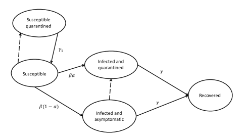
Figure 1: A transition diagram of an SIR model with contact tracing and isolation. Spontaneous transitions are shown in solid arrows. Dashed arrows denote transitions that are caused by spontaneous transitions. Specifically, as a susceptible individual becomes infected, a fraction $\eta$ of his or her neighbors are tested. His or her susceptible neighbors (resp. asymptomatic neighbors) are isolated. This causes a dashed transition from the susceptible state to the susceptible and quarantined state (resp. infected and quarantined state). The transition rates of spontaneous transitions are shown besides the corresponding arrows.

We apply a degree-based approximation to the SIR model with contact tracing and isolation. Degree-based approximation is a well known technique to study epidemic spreading in a contact graph [10, 11, 12, 13]. The following is a list of variables that will be used in the analysis. Note that excess degrees are defined to be the degree of a vertex reached by traversing an edge. The excess degree does not include the traversed edge.

• $s_{k}(t)$: The fraction of nodes that are in state Susceptible at time $t$ among all nodes that have excess degree $k$.

• $q^{S}_{k}(t)$: The fraction of nodes that are in state Susceptible and quarantined at time $t$ among all nodes with excess degree $k$.

• $x_{k}(t)$: The fraction of nodes that are in state Infected and asymptomatic at time $t$ among all nodes with excess degree $k$.

• $q^{I}_{k}(t)$: The fraction of nodes that are in state Infected and quarantined at time $t$ among all nodes with excess degree $k$.

• $r_{k}(t)$: The fraction of nodes with excess degree $k$ that are in the recovered state.

We remark that the quantities above satisfy an equality

$$s_{k}(t)+q^{S}_{k}(t)+x_{k}(t)+q^{I}_{k}(t)+r_{k}(t)=1$$ (1)

for all $k$ and all $t$.

Let $\{p_{k},k=0,1,2,\ldots\}$ be the degree distribution of a randomly selected vertex. Let $\{w_{k},k=0,1,2,\ldots\}$ be the excess degree distribution of a vertex reached by traversing a randomly selected edge. That is, if one traverses along a randomly selected edge from one node to a neighbor of the node, then $w_{k}$ is the probability that this neighbor has $k$ edges, not including the traversed edge. Let $g_{0}(x)$ and $g_{1}(x)$ be the probability generating functions of degree distribution $\{p_{k},k\geq 0\}$ and excess degree distribution $\{w_{k},k\geq 0\}$, respectively. That is,

$$g_{0}(x) =\sum_{k=0}^{\infty}p_{k}x^{k},$$ (2)

$$g_{1}(x) =\sum_{k=0}^{\infty}w_{k}x^{k}.$$ (3)

Let $K_{0}$ and $K_{1}$ denote the expectation of distributions of $\{p_{k},k\geq 0\}$ and $\{w_{k},k\geq 0\}$, respectively. That is,

$$K_{0} =\sum_{k=0}^{\infty}kp_{k}=g_{0}^{\prime}(1),$$ (4)

$$K_{1} =\sum_{k=0}^{\infty}kw_{k}=g_{1}^{\prime}(1).$$ (5)

Let

$$v(t)=\sum_{k=0}^{\infty}w_{k}x_{k}(t).$$ (6)

Then, $v(t)$ is the probability that a vertex reached by traversing a randomly selected edge is infected and not isolated. We now derive a system of differential equations that link $s_{k}(t)$, $q^{S}_{k}(t)$, $x_{k}(t)$, $q^{I}_{k}(t)$ and $r_{k}(t)$. First,

$$\frac{d}{dt}s_{k}(t)=-\beta kvs_{k}-\sum_{j=0}^{\infty}\left[\alpha\sum_{\ell=1}^{\infty}\beta\ell vs_{\ell}p_{\ell}\right]p_{j}j\eta s_{k}+\gamma_{1}q^{S}_{k}.$$ (7)

The left hand side of (7) is the rate of change in the fraction of susceptible nodes with degree $k$. The first term on the right side is the rate of change in the fraction of susceptible nodes with degree $k$ due to infected but not isolated neighbors. Each of such a susceptible node has $k$ neighbors. Each neighbor is infected with probability $v(t)$ which is defined in (6). We thus have the first term on the right side. The first term also appears in the degree based approximation of the standard SI, SIR and SIS models. We refer the reader to Newman [9, p. 659, 665 and 671]. The fraction of vertices that have degree $k$, are isolated and susceptible is $q^{S}_{k}(t)$. With rate $\gamma_{1}$, isolated and susceptible individuals are released from isolation and return to susceptible state. Thus, we have the third term on the right side of (7). We now explain the second term. The fraction of newly infected individuals at time $t$ that have degree $k$ is $\beta kvs_{k}$. Thus, the total fraction of newly infected individuals at time $t$ is

$$\sum_{k=1}^{\infty}\beta kvs_{k}p_{k}.$$

Among those who are newly infected, a fraction $\alpha$ of individuals show symptoms and are quarantined and isolated. A fraction $1-\alpha$ of individuals are asymptomatic and are not isolated. Thus, the fraction of newly infected individuals who show symptoms is

$$\alpha\sum_{k=1}^{\infty}\beta kvs_{k}p_{k}.$$

Those who show symptoms will be quarantined and isolated. The fraction of newly infected individuals who are isolated and have degree $j$ is

$$\left(\alpha\sum_{k=1}^{\infty}\beta kvs_{k}p_{k}\right)p_{j}.$$

Each individual in the preceding quantity has $j$ neighbors. Each neighbor is isolated with probability $\eta$. Thus, the fraction of newly isolated individuals is

$$\sum_{j=0}^{\infty}\left(\alpha\sum_{k=1}^{\infty}\beta kvs_{k}p_{k}\right)p_{j}j\eta.$$ (8)

These isolated neighbors are susceptible and have degree $\ell$ with probability $s_{\ell}(t)$. Thus, the fraction of newly isolated and susceptible individuals who have degree $\ell$ is

$$\sum_{j=0}^{\infty}\left(\alpha\sum_{k=1}^{\infty}\beta kvs_{k}p_{k}\right)p_{j}j\eta s_{\ell}(t).$$ (9)

This is the second term on the right side of (7).

With similar arguments one can derive differential equations for $q^{S}_{k}(t)$, $x_{k}(t)$, $q^{I}_{k}(t)$ and $r_{k}(t)$. They are listed as follows.

$$\frac{d}{dt}q^{S}_{k}(t) =\sum_{j=0}^{\infty}\left[\alpha\sum_{\ell=1}^{\infty}\beta\ell vs_{\ell}p_{\ell}\right]p_{j}j\eta s_{k}-\gamma_{1}q^{S}_{k},$$ (10)

$$\frac{d}{dt}x_{k}(t) =(1-\alpha)\beta kvs_{k}-\sum_{j=0}^{\infty}\left[\alpha\sum_{\ell=1}^{\infty}\beta\ell vs_{\ell}p_{\ell}\right]p_{j}j\eta x_{k}$$

$$\quad-\gamma x_{k},$$ (11)

$$\frac{d}{dt}q^{I}_{k}(t) =\alpha\beta kvs_{k}+\sum_{j=0}^{\infty}\left[\alpha\sum_{\ell=1}^{\infty}\beta\ell vs_{\ell}p_{\ell}\right]p_{j}j\eta x_{k}$$

$$\quad-\gamma q^{I}_{k},$$ (12)

$$\frac{d}{dt}r_{k}(t) =\gamma x_{k}+\gamma q^{I}_{k}.$$ (13)

The derivation of the second term on the right side of (11) and (12) is similar. The fraction of newly isolated individuals is given in (8). The fraction of isolated individuals who are infected (asymptomatically) and have degree $\ell$ is the quantity in (8) multiplied with $x_{\ell}(t)$. This gives the second term on the right side of (11) and (12). We can simplify the second term on the right side of (7) and (11), respectively. Eqs. (7) and (10)-(12) become

$$\frac{d}{dt}s_{k}(t) =-\beta kvs_{k}-\alpha\beta vK_{0}\eta\left[\sum_{\ell=1}^{\infty}\ell s_{\ell}p_{\ell}\right]s_{k}+\gamma_{1}q^{S}_{k},$$ (14)

$$\frac{d}{dt}q^{S}_{k}(t) =\alpha\beta vK_{0}\eta\left[\sum_{\ell=1}^{\infty}\ell s_{\ell}p_{\ell}\right]s_{k}-\gamma_{1}q^{S}_{k},$$ (15)

$$\frac{d}{dt}x_{k}(t) =(1-\alpha)\beta kvs_{k}-\alpha\beta vK_{0}\eta\left[\sum_{\ell=1}^{\infty}\ell s_{\ell}p_{\ell}\right]x_{k}-\gamma x_{k},$$ (16)

$$\frac{d}{dt}q^{I}_{k}(t) =\alpha\beta kvs_{k}+\alpha\beta vK_{0}\eta\left[\sum_{\ell=1}^{\infty}\ell s_{\ell}p_{\ell}\right]x_{k}-\gamma q^{I}_{k},$$ (17)

where $K_{0}$ defined in (4) denotes the mean degree of a randomly selected vertex. Unlike the differential equations for the classical SIR model which can be analytically solved, the presence of the terms such as the second term on the right side of (14) makes (14)-(17) and (13) very difficult. They can only be solved numerically. Once $\{s_{k}(t),0\leq k<\infty\}$ are obtained, one can calculate

$$s(t)\stackrel{{\scriptstyle\scriptstyle\rm def}}{{=}}\sum_{k=0}^{\infty}p_{k}s_{k}(t).$$ (18)

This is the probability that a randomly selected vertex is susceptible. Probabilities that a randomly selected vertex is infected and quarantined, susceptible and quarantined, infected but asymptomatic, or recovered can be obtained similarly.

In Section 3, we present an early-time analysis. Numerical solution of the system is also difficult. Suppose that we truncate the excess degree distribution to $[0,K_{\mbox{\small max}}]$. For each degree value, there are five differential equations. Thus, the dimension of the system in (7) and (10)-(13) is $5(1+K_{\mbox{\small max}})$. We propose an approximate analysis in Section 4 to reduce the numerical complexity.

3 Early Time Analysis

In this section we present an early time analysis of the system in (7), (10)-(13).

We assume that initially there is small number of infected individuals and that most individuals are susceptible. That is, we assume that

$$s_{k}(0)=1-\epsilon,\quad x_{k}(0)=\epsilon,$$

$$q^{S}_{k}(0)=q^{I}(0)=r(0)=0,$$

for some small number $\epsilon\approx 0$. Substituting $s_{k}(t)\approx 1-\epsilon$ in Eq. (16), multiplying the two sides of (16) with $w_{k}$ and summing from $k=0$ to infinity, we obtain

$$\frac{dv}{dt}=[(1-\alpha)\beta g_{1}^{\prime}(1)(1-\epsilon)-\gamma]v-\alpha\beta\eta K_{0}^{2}(1-\epsilon)v^{2}.$$

This differential equation is separable and can be rewritten as

$$\frac{dv}{v(c_{2}-c_{1}v)}=dt,$$ (19)

where

$$c_{1} =\alpha\beta\eta K_{0}^{2}(1-\epsilon),$$ (20)

$$c_{2} =(1-\alpha)\beta K_{1}(1-\epsilon)-\gamma,$$ (21)

and $K_{1}=g_{1}^{\prime}(1)$ is defined in (5). The solution of (19) is

$$v(t)=\frac{c_{2}D_{1}e^{c_{2}t}}{1+c_{1}D_{1}e^{c_{2}t}},$$ (22)

where $D_{1}$ is a constant determined by the initial condition $v(0)=\epsilon$, i.e.

$$D_{1}=\frac{\epsilon}{c_{2}-c_{1}\epsilon}.$$

If $c_{2}<0$, $v(t)\to 0$ as $t\to\infty$. In this case, the epidemic dies down. On the other hand, if $c_{2}>0$, $v(t)\to c_{2}/c_{1}$ as $t\to\infty$. In this case, a significant fraction of population will be infected with the disease. Since $\epsilon$ is arbitrary, the condition for the epidemic to die down is

$$(1-\alpha)\beta K_{1}<\gamma$$

and the condition for the epidemic to grow significantly is

$$(1-\alpha)\beta K_{1}>\gamma.$$

Define

$$R_{0}=\frac{(1-\alpha)\beta K_{1}}{\gamma}.$$ (23)

The epidemic threshold is $R_{0}=1$, which separates the shrinking and growing regimes of the epidemic. $R_{0}$ is the basic reproduction number of the disease. It is the expected number of asymptomatic patients passed on by an infected individual during his/her infection. It is interesting to see that $R_{0}$ depends only on the parameters of the disease, and not on parameters $\eta$ and $\gamma_{1}$ of the contact tracing and isolation policy.

4 Approximate Analysis

In this section we present an approximation to reduce the dimension of the system in (7) and (10)-(13). We assume that

$$s_{k}(t)=(u(t))^{k}$$ (24)

for some unknown function $u(t)$. Note that for the classical SI model and the SIR model, (24) holds for function $u(t)$ that depends on $v(t)$ and $\{r_{k}(t),k\geq 0\}$, respectively. We refer the reader to (17.60) and (17.87) in Newman [9]. In our model, (24) is only an approximation. However, it greatly simplifies the second term on the right side of (14) that was caused by contact tracing and isolation.

Define

$$q^{S}(t) =\sum_{k=0}^{\infty}w_{k}q^{S}_{k}(t),$$ (25)

$$q^{I}(t) =\sum_{k=0}^{\infty}w_{k}q^{I}_{k}(t),$$ (26)

$$r(t) =\sum_{k=0}^{\infty}w_{k}r_{k}(t).$$ (27)

Substituting (24) into (7), one gets

$$ku^{k-1}\frac{du}{dt}=-\beta kvu^{k}-\alpha\beta v\left(\sum_{\ell=1}^{\infty}\ell u^{\ell}p_{\ell}\right)K_{0}\eta u^{k}+\gamma_{1}q^{S}_{k}.$$ (28)

Since

$$\sum_{\ell=1}^{\infty}\ell u^{\ell}p_{\ell} =u\sum_{\ell=1}^{\infty}\ell u^{\ell-1}p_{\ell}$$

$$=u\frac{d\left(\sum_{\ell=1}^{\infty}u^{\ell}p_{\ell}\right)}{du}$$

$$=ug_{0}^{\prime}(u),$$

Eq. (28) becomes

$$ku^{k-1}\frac{du}{dt}=-\beta kvu^{k}-\alpha\beta vK_{0}\eta ug_{0}^{\prime}(u)u^{k}+\gamma_{1}q^{S}_{k}.$$

Multiplying the preceding with $w_{k}$, summing from $k=0$ to infinity and manipulating algebraically, one gets

$$\frac{du}{dt} =-\beta vu-\alpha\beta vK_{0}\eta ug_{0}^{\prime}(u)\frac{g_{1}(u)}{g_{1}^{\prime}(u)}+\gamma_{1}\frac{q^{S}}{g_{1}^{\prime}(u)}.$$ (29)

Similarly, we multiply the two sides of (10)-(13) with $w_{k}$ and sum from $k=0$ to infinity. We obtain

$$\frac{dq^{S}}{dt} =\alpha\beta K_{0}\eta vug_{1}(u)g_{0}^{\prime}(u)-\gamma_{1}q^{S},$$ (30)

$$\frac{dv}{dt} =(1-\alpha)\beta vug_{1}^{\prime}(u)-\alpha\beta K_{0}\eta v^{2}ug_{0}^{\prime}(u)-\gamma v,$$ (31)

$$\frac{dq^{I}}{dt} =\alpha\beta vug_{1}^{\prime}(u)+\alpha\beta K_{0}\eta v^{2}ug_{0}^{\prime}(u)-\gamma q^{I},$$ (32)

$$\frac{dr}{dt} =\gamma(v+q^{I}).$$ (33)

Eqs. (29), (30)-(33) form a nonlinear system of differential equations for unknown functions $u(t)$, $q^{S}(t)$, $v(t)$, $q^{I}(t)$ and $r(t)$ subject to initial conditions $u(0),v(0),q^{S}(0),q^{I}(0)$ and $r(0)$. In Section 6 we numerically solve this system and compare with the numerical solution of the system in (14)-(17) and (13).

Once functions $u(t)$ and $v(t)$ are obtained, we can determine sequences of functions $s_{k}(t)$, $q^{S}_{k}(t)$, $x_{k}(t)$, $q^{I}_{k}(t)$ and $r_{k}(t)$ for $k\geq 0$ in a straight forward manner. First, $s_{k}(t)$ can be directly obtained in (24) using $u(t)$. Differential equations involving with $q^{S}_{k}(t)$ and $q^{I}_{k}(t)$ are linear and can be solving using the integrating factor technique. Function $r_{k}(t)$ can be obtained by a direct integration.

5 Stability Analysis

In this section we present a stability analysis of the nonlinear system in (29) and (30)-(33). Note that once functions $u(t)$, $q^{S}(t)$ and $v(t)$ are obtained, functions $q^{I}(t)$ and $r(t)$ can be obtained using the technique of integrating factors and direct integration, respectively. Thus, one just needs to consider the nonlinear system in (29), (30) and (31), in which there are only three unknown functions. In order to facilitate our presentation in matrix and vector forms, we use symbols $y_{1},y_{2}$, and $y_{3}$ to denote $u,q^{S}$, and $v$, respectively. Thus, $y_{1}(t),y_{2}(t)$ and $y_{3}(t)$ denote $u(t),q^{S}(t)$ and $v(t)$, respectively. We rewrite (29), (30) and (31) using new symbols, i.e.

$$y_{1}^{\prime} =-\beta y_{3}y_{1}-\alpha\beta K_{0}\eta y_{3}y_{1}g_{0}^{\prime}(y_{1})\frac{g_{1}(y_{1})}{g_{1}^{\prime}(y_{1})}+\gamma_{1}\frac{y_{2}}{g_{1}^{\prime}(y_{1})},$$ (34)

$$y_{2}^{\prime} =\alpha\beta K_{0}\eta y_{3}y_{1}g_{1}(y_{1})g_{0}^{\prime}(y_{1})-\gamma_{1}y_{2},$$

$$y_{3}^{\prime} =(1-\alpha)\beta y_{3}y_{1}g_{1}^{\prime}(y_{1})-\alpha\beta K_{0}\eta y_{3}^{2}y_{1}g_{0}^{\prime}(y_{1})-\gamma y_{3}.$$

Denote the right side of the equations above by $f_{1},f_{2}$ and $f_{3}$, respectively. We have

$$y_{1}^{\prime} =f_{1}(y_{1},y_{2},y_{3}),$$

$$y_{2}^{\prime} =f_{2}(y_{1},y_{2},y_{3}),$$ (35)

$$y_{3}^{\prime} =f_{3}(y_{1},y_{2},y_{3}).$$

The preceding can be expressed in terms of vectors, i.e.

$${\mbox{\boldmath$x$}}^{\prime}={\mbox{\boldmath$f$}}({\mbox{\boldmath$x$}}),$$ (36)

where we use boldface letters to denote vectors and matrices. We are interested in the stability of equilibrium point $(y_{1},y_{2},y_{3})=(\xi,0,0)$. Recall the definition of the Jacobian matrix of a system in the form of (36). The $(i,j)$ entry of the Jacobian matrix is defined to be

$$\left({\mbox{\boldmath$J$}}(\xi,0,0)\right)_{i,j}=\left.\frac{\partial f_{i}}{\partial x_{j}}\right|_{{\mbox{\boldmath\scriptsize$x$}}=(\xi,0,0)}.$$

The Jacobian matrix of the functions on the right side of (35) evaluated at $(\xi,0,0)$ is

$${\mbox{\boldmath$J$}}(\xi,0,0)=$$

$$\left(\begin{array}[]{ccc}0&\gamma_{1}/g_{1}^{\prime}(\xi)&-\beta\xi-\alpha\beta K_{0}\eta\xi g_{0}^{\prime}(\xi)g_{1}(\xi)/g_{1}^{\prime}(\xi)\\ 0&-\gamma_{1}&\alpha\beta K_{0}\eta\xi g_{0}^{\prime}(\xi)g_{1}(\xi)\\ 0&0&(1-\alpha)\beta\xi g_{1}^{\prime}(\xi)-\gamma\end{array}\right).$$ (40)

Since ${\mbox{\boldmath$J$}}(\xi,0,0)$ is singular, the nonlinear system is not almost linear in the neighborhood of $(\xi,0,0)$. Thus, the general stability theory of almost linear systems can not be applied here. In addition, in almost linear systems equilibrium points are isolated. In our problem, equilibrium points are not isolated. Any point on the $y_{1}$ axis is an equilibrium point. These characteristics make each nonlinear system with singular Jacobian matrices unique. Each problem needs a dedicated analysis. To see that our nonlinear system with Jacobian matrix in (40) is not almost linear, note that since the Jacobian matrix is singular, one can apply elementary row operations to convert all entries in the first row to zero. Thus, the dominant terms in the first equation are not linear. Rather, the right side of the first equation is dominated by quadratic terms.

Since probability generating functions are power series, functions $f_{i},i=1,2,3,$ have continuous derivatives of all orders. Thus, one can apply Taylor expansion to $f_{i},i=1,2,3,$ around the equilibrium point ${\mbox{\boldmath$x$}}_{e}=(\xi,0,0)^{T}$, where symbol $T$ denotes the transpose operation. For functions $f_{2}$ and $f_{3}$, we keep only the linear terms in their Taylor expansions. For function $f_{1}$, we keep both the linear term and the quadratic term. In matrix form, we have

$${\mbox{\boldmath$x$}}^{\prime}={\mbox{\boldmath$J$}}({\mbox{\boldmath$x$}}_{e})({\mbox{\boldmath$x$}}-{\mbox{\boldmath$x$}}_{e})+\left[\begin{array}[]{c}({\mbox{\boldmath$x$}}-{\mbox{\boldmath$x$}}_{e})^{T}{\mbox{\boldmath$H$}}({\mbox{\boldmath$x$}}_{e})({\mbox{\boldmath$x$}}-{\mbox{\boldmath$x$}}_{e})\\ 0\\ 0\end{array}\right],$$ (41)

where ${\mbox{\boldmath$H$}}({\mbox{\boldmath$x$}}_{e})$ is the Hessian matrix evaluated at point ${\mbox{\boldmath$x$}}_{e}$. The $(i,j)$ entry of ${\mbox{\boldmath$H$}}({\mbox{\boldmath$x$}}_{e})$ is

$$\frac{\partial^{2}f_{1}({\mbox{\boldmath$x$}})}{\partial x_{i}\partial x_{j}},\qquad 1\leq i,j\leq 3.$$

It is straight forward to show that the Hessian matrix of the function on the right side of (34) is

$${\mbox{\boldmath$H$}}({\mbox{\boldmath$x$}}_{e})=\left(\begin{array}[]{ccc}0&A&B\\ A&0&0\\ B&0&0\end{array}\right),$$ (42)

where $A$ and $B$ are defined as

$$A =\frac{-\gamma_{1}g_{1}^{\prime\prime}(\xi)}{(g_{1}^{\prime}(\xi))^{2}},$$

$$B =-\beta-\alpha\beta K_{0}\eta\left(g_{0}^{\prime}(\xi)\frac{g_{1}(\xi)}{g_{1}^{\prime}(\xi)}+\xi g_{0}^{\prime\prime}(\xi)\frac{g_{1}(\xi)}{g_{1}^{\prime}(\xi)}+\right.$$

$$\quad\left.+\xi g_{0}^{\prime}(\xi)\frac{(-1)g_{1}^{\prime\prime}(\xi)g_{1}(\xi)}{(g_{1}^{\prime}(\xi))^{2}}+\xi g_{0}^{\prime}(\xi)\right).$$

Typically, one considers a “translated system” of a nonlinear system in order to simplify notations. That is, let

$$\tilde{\mbox{\boldmath$x$}}={\mbox{\boldmath$x$}}-{\mbox{\boldmath$x$}}_{e}.$$

Rewrite (41) in terms of $\tilde{\mbox{\boldmath$x$}}$, i.e.

$$\tilde{\mbox{\boldmath$x$}}^{\prime}={\mbox{\boldmath$J$}}({\mbox{\boldmath$x$}}_{e})\tilde{\mbox{\boldmath$x$}}+\left[\begin{array}[]{c}\tilde{\mbox{\boldmath$x$}}^{T}{\mbox{\boldmath$H$}}({\mbox{\boldmath$x$}}_{e})\tilde{\mbox{\boldmath$x$}}\\ 0\\ 0\end{array}\right],$$ (43)

Note that the equilibrium point ${\mbox{\boldmath$x$}}_{e}$ is translated to the origin in the translated system.

Now we consider system (43) with initial condition

$$(\tilde{y}_{1}(0),\tilde{y}_{2}(0),\tilde{y}_{3}(0))=(\epsilon,\epsilon,\epsilon)$$

for some small positive number $\epsilon$. Note the upper triangular form of the Jacobian matrix in (40). We solve $\tilde{x}_{i}(t)$ successively starting from $i=3$. From (43) and (40), we have

$$\tilde{y}_{3}^{\prime}=a\tilde{y}_{3},$$ (44)

where

$$a=(1-\alpha)\beta\xi g_{1}^{\prime}(\xi)-\gamma.$$ (45)

Thus,

$$\tilde{y}_{3}(t)=\epsilon e^{at}.$$ (46)

If $a<0$, $\tilde{y}_{3}(t)\to 0$. If $a>0$, $\tilde{y}_{3}(t)\to\infty$. Now we substitute (46) into the second equation in (43) and obtain

$$\tilde{y}_{2}^{\prime}=-\gamma_{1}\tilde{y}_{2}+\alpha\beta K_{0}\eta\xi g_{0}^{\prime}(\xi)g_{1}(\xi)\epsilon e^{at}.$$

This is a linear differential equation and can be solved using the technique of integrating factors. The solution is

$$\tilde{y}_{2}(t)=(he^{at}+(1-h)e^{-\gamma_{1}t})\epsilon,$$ (47)

where

$$h =\frac{\alpha\beta K_{0}\eta\xi g_{0}^{\prime}(\xi)g_{1}(\xi)}{a+\gamma_{1}}.$$

From (47), if $a<0$, $\tilde{y}_{2}(t)\to 0$. If $a>0$, $\tilde{y}_{2}(t)\to\infty$. Finally, we substitute (46) and (47) into (41), algebraically simplify and obtain

$$\tilde{y}_{1}^{\prime}=\left(d_{1}e^{at}+d_{2}e^{-\gamma_{1}t}\right)\epsilon\tilde{y}_{1}+\left(d_{3}e^{at}+d_{4}e^{-\gamma_{1}t}\right)\epsilon,$$ (48)

where

$$d_{1} =Ah+B,$$

$$d_{2} =A(1-h),$$

$$d_{3} =\frac{h\gamma_{1}}{g_{1}^{\prime}(\xi)}-\left(\beta\xi+\alpha\beta K_{0}\eta\xi g_{0}^{\prime}(\xi)\frac{g_{1}(\xi)}{g_{1}^{\prime}(\xi)}\right),$$

$$d_{4} =\frac{(1-h)\gamma_{1}}{g_{1}^{\prime}(\xi)}.$$

Eq. (48) is linear and its solution is

$$\tilde{y}_{1}(t)=\exp\left(\frac{d_{1}}{a}\epsilon e^{at}-\frac{d_{2}}{\gamma_{1}}\epsilon e^{-\gamma_{1}t}\right)\Biggl{(}\frac{\epsilon}{\exp\left(\frac{d_{1}\epsilon}{a}-\frac{d_{2}\epsilon}{\gamma_{1}}\right)}+$$

$$\quad\int_{0}^{t}\exp\left(-\frac{d_{1}\epsilon}{a}e^{ay}+\frac{d_{2}\epsilon}{\gamma_{1}}e^{-\gamma_{1}y}\right)\left(d_{3}\epsilon e^{ay}+d_{4}\epsilon e^{-\gamma_{1}y}\right)\,dy\Biggr{)}.$$ (49)

Clearly, if $a>0$, it follows from (49) that $\tilde{y}_{1}(t)\to\infty$. On the other hand, if $a<0$, as $t\to\infty$,

$$\tilde{y}_{1}(t) \to\epsilon\exp\left(-\frac{d_{1}\epsilon}{a}+\frac{d_{2}\epsilon}{\gamma_{1}}\right)+$$

$$\quad\int_{0}^{\infty}\exp\left(-\frac{d_{1}\epsilon}{a}e^{ay}+\frac{d_{1}\epsilon}{\gamma_{1}}e^{-\gamma_{1}y}\right)\times$$

$$\qquad\quad\left(d_{3}\epsilon e^{ay}+d_{4}\epsilon e^{-\gamma_{1}y}\right)\,dy.$$ (50)

We now present an upper bound and a lower bound for the integral on the right side of (50). Since $\exp(\omega t)$ is increasing with $\omega$ for any $t$, we have

$$e^{at}\leq e^{Mt},\quad e^{-\gamma_{1}t}\leq e^{Mt},$$

$$e^{at}\geq e^{mt},\quad e^{-\gamma_{1}t}\geq e^{mt},$$

where

$$M =\max(a,-\gamma_{1}),$$

$$m =\min(a,-\gamma_{1}).$$

The integral on the right side of (50) is bounded above by $U\epsilon$, where

$$U =\int_{0}^{\infty}\exp\left(\left|\frac{d_{1}\epsilon}{a}\right|e^{my}+\left|\frac{d_{2}\epsilon}{\gamma_{1}}\right|e^{my}\right)(|d_{3}|+|d_{4}|)e^{my}\,dy$$

$$=\frac{|d_{3}|+|d_{4}|}{m}\frac{1-\exp\left(\left|\frac{d_{1}\epsilon}{a}\right|+\left|\frac{d_{2}\epsilon}{\gamma_{1}}\right|\right)}{\left(\left|\frac{d_{1}}{a}\right|+\left|\frac{d_{2}}{\gamma_{1}}\right|\right)\epsilon}$$

$$\approx\frac{|d_{3}|+|d_{4}|}{|m|}.$$ (51)

With a similar analysis, we obtain a lower bound $L\epsilon$ of the integral on the right side of (50), where

$$L=-\frac{|d_{3}|+|d_{4}|}{|m|}.$$ (52)

The first term on the right side of (50) is approximately equal to $\epsilon$. Thus, from (51), it follows that

$$\tilde{y}_{1}(t)\to\xi^{*}\in(\epsilon(1+L),\epsilon(1+U)).$$ (53)

In conclusion, starting initially from $(\epsilon,\epsilon,\epsilon)$, the solution $(y_{1}(t),y_{2}(t),y_{3}(t))$ converges to $(\xi+\xi^{*},0,0)$, where $\xi^{*}$ satisfies (53). On the other hand, if $a>0$, $y_{i}(t)\to\infty$ for $i=1,2,3$, as $t\to\infty$. Note that $a$ depends only on the parameters of the disease and the generating function of the excess degree distribution. It does not depend on the parameters of the contact tracing and isolation policy.

6 Numerical and Simulation Results

We present numerical and simulation results in this section. Numerical solution of Eqs. (13)-(17) is presented in Section 6.1. We simulate the SIR model with contact tracing and isolation on five real-world networks. The simulation results are shown in Section 6.2.

6.1 Solution of Differential Equations

Given a degree distribution $\{p_{k},k\geq 0\}$, we determine its corresponding excess degree distribution $\{w_{k},k\geq 0\}$ according to

$$w_{k}=\frac{(k+1)p_{k+1}}{K_{0}}$$

for $k\geq 0$ [9]. Recall that $K_{0}$ is the expectation of degree distribution $\{p_{k},k\geq 0\}$. We truncate the two degree distributions properly such that the error is small. We use Matlab differential equations solver to numerically solve Eqs. (13)-(17) for Poisson degree distributions and power law degree distributions. We assume that the initial condition is $s_{k}(0)=1-10^{-3}$, $x_{k}(0)=10^{-3}$ and $q^{S}_{k}(0)=q^{I}_{k}(0)=r_{k}(0)=0$. We then apply (18) to compute the overall probability of recovery. For Poisson degree distributions, we assume that the mean degree is 25. For power law degree distribution, we assume that the exponent of the distribution is $-2.5$. We truncate both distributions to range $[0,1000]$. Values of other parameters are shown in Table I. We show the probability of recovery for the power law degree distribution in Fig. 2 for several values of $\eta$. Note that the curve with $\eta=0$ corresponds to the epidemic without contact tracing and isolation. This figure shows that the contact tracing and isolation is effective in containing the epidemic. In Fig. 3 we show $q^{S}(t)$ for several values of $\eta$. From this figure, we see that while contact tracing and isolation is effective in containing the epidemic, it comes at a cost. The contact tracing and isolation can be detrimental to the normal function of a society. With a strict isolation rule corresponding to a large value of $\eta$, we see from Fig. 3 that more than 8% of the total population are isolated. However, these isolated individuals are susceptible. We show how $r(t)$ and $q^{S}(t)$ vary with $\alpha$ in Figs. 4 and 5. In the calculation of these two figures, the value of $\eta$ is 0.5.

parameter	$\alpha$	$\beta$	$\gamma$	$\gamma_{1}$	$\eta$
value	0.4	0.15	0.1	0.1	0.5

TABLE I: Parameter values used in numerical studies.

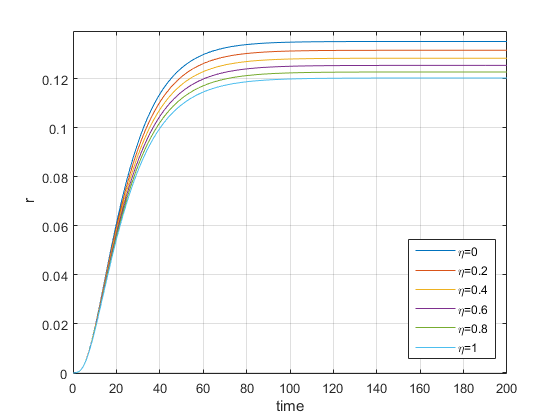
Figure 2: Probability of recovery as a function of time for several values of $\eta$.

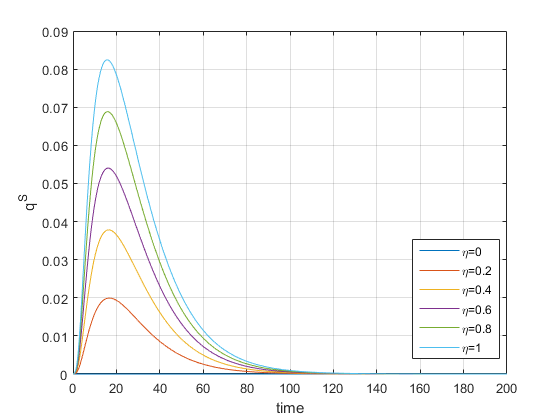
Figure 3: Probability of isolated individuals who are susceptible as a function of time for several values of $\eta$.

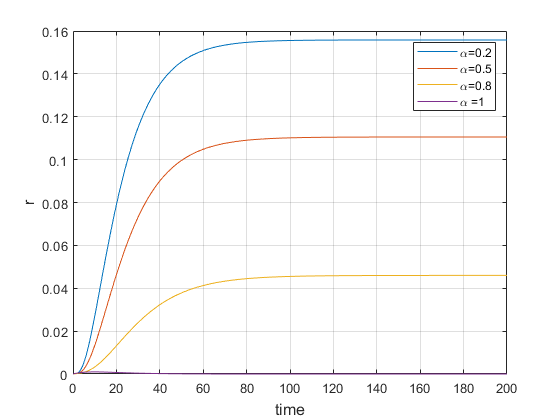
Figure 4: Probability of recovery as a function of time for several values of $\alpha$.

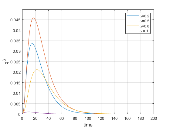
Figure 5: Probability of isolated individuals who are susceptible as a function of time for several values of $\alpha$.

We now present numerical studies of the early-time analysis presented in Section 3. We calculate a ratio by dividing the result of the early-time analysis by that of the exact numerical result. The ratios are shown in Fig. 6. As expected, the early time analysis is accurate when time is small and starts to deviate when time is getting large.

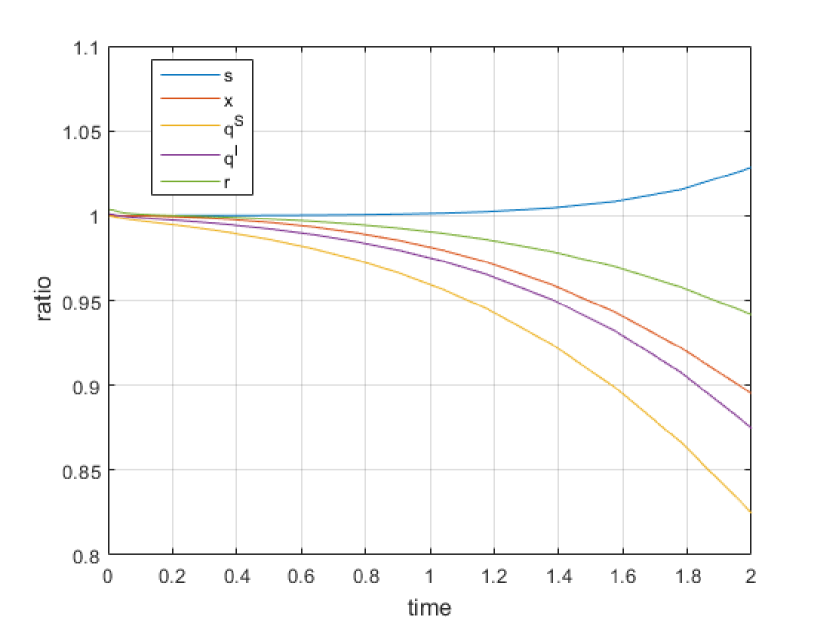
Figure 6: Early time analysis. The ratios of early time analysis divided by that of the exact numerical result are shown.

We use Matlab to numerically solve Eqs. (29)-(33). We set the initial condition as follows. Let $v(0)=10^{-3}$, $q^{S}(0)=q^{I}(0)=r(0)=0$, and $u(0)=g_{1}^{-1}(1-10^{-3})$, where $g_{1}^{-1}$ is the inverse function of the probability generating function $g_{1}$. We calculate a ratio by dividing the result of the approximate analysis by that of the exact numerical result. The ratios are shown in Fig. 7. We see that the approximation method works quite well. The errors are typically within five percents. We also study the approximate analysis of the power law degree distribution with exponent $-2.5$. The ratios are shown in Fig. 8. The errors in this case are higher, but are within a reasonable range. At late time of the epidemic, the errors corresponding to $q^{S}(t)$ and $q^{I}(t)$ can be twenty percents. We show the exact analysis and the approximate analysis of $x(t)$, $q^{S}(t)$ and $q^{I}(t)$ in Fig. 9. We see that the result of exact analysis and that of the approximate analysis are very close in early time and mid time. At late time, the difference between the two analyses are visible. However, the values of $x(t)$, $q^{S}(t)$ and $q^{I}(t)$ are very small and they are less significant to the epidemics.

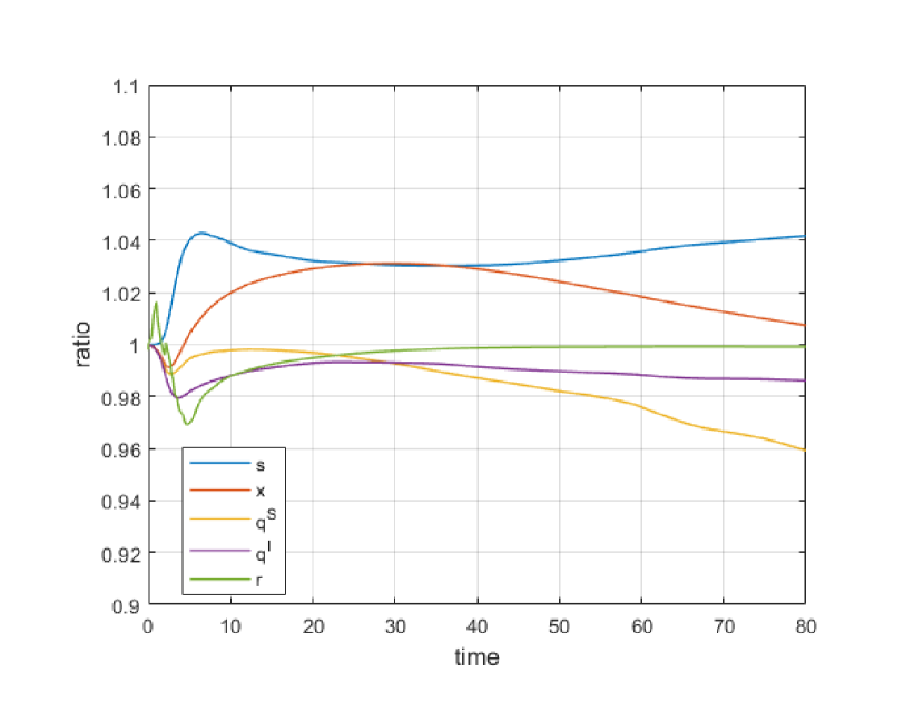
Figure 7: Approximate analysis. The ratios of approximate analysis divided by that of the exact numerical result are shown. A randomly selected vertex has a Poisson degree distribution.

Figure 8: Approximate analysis. The ratios of approximate analysis divided by that of the exact numerical result are shown. A randomly selected vertex has a power law degree distribution.

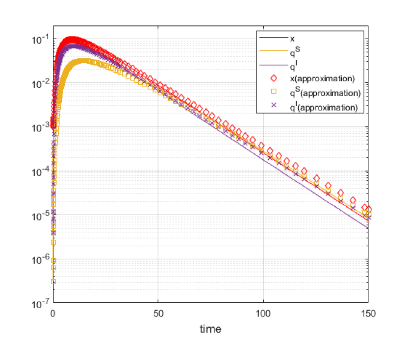
Figure 9: Values of $x(t)$, $q^{S}(t)$ and $q^{I}(t)$ obtained by exact numerical analysis and approximate analysis. Degrees have a power law distribution with exponent $-2.5$.

6.2 Simulation of Real-world Networks

We analyze contact tracing and isolation using configuration network models. Configuration models are mathematically simple, but lack some important characteristics such as clustering and degree correlations. It is known that real-world networks possess these characteristics [9] and it is known that these characteristics have non-neglectable impacts to many networking problems [24]. It is well known that a group of individuals with close contacts with each other, such as members in a household or workmates in an office, are likely to contract the disease if one in the group does [14, 15]. In this section we study the SIR model with contact tracing and isolation on real-world networks by simulation. We simulate a more general contact tracing and isolation policy. In our simulation model there are two types of edges. The first type of edges connects two close contacts. The disease has a higher transmission rate across edges across the first type of edges. The second type of edges connects two normal contacts. We refer the reader to Fig. 10 for a graphical illustration. Suppose that vertex $A$ is infected and shows symptoms. We assume that the contact tracing and isolation policy quarantines and isolates all $A$’s close contacts, i.e. $B_{1},B_{2},\ldots,B_{i}$. In addition, the policy isolates a fraction $\eta$ of $A$’s normal contacts. Specifically, each $C_{k}$, for $1\leq k\leq j$, is isolated with probability $\eta$.

To the best of our efforts, we have not been able to find datasets of real-world networks, in which edges are marked according to whether they connect two close contacts or two normal contacts. Tie strength is a fundamental topic in sociology [25]. Strong ties generally refer to edges corresponding to closer friendships or greater frequency of interactions. On the other hand, weak ties generally refer to edges connecting two acquaintances [26]. Given a social graph, there have been efforts to mark the strengths of the edges in the graph [27, 28]. Particularly, Onnela et al. [27] studied a network formed by communications among cellular phones over an 18-week period. Onnela et al. found tie strengths and neighborhood overlap are highly correlated. The neighborhood overlap of an edge connecting vertices $A$ and $B$ is defined as the ratio

$$\frac{|N_{A}\cap N_{B}|}{|N_{A}\cup N_{B}-\{A,B\}|},$$ (54)

where $N_{A}$ and $N_{B}$ denote the sets of $A$ and $B$’s neighbors, respectively. The denominator of (54) is the number of $A$’s neighbors and $B$’s neighbors. However, $A$ and $B$ are excluded. Clearly, the neighbor overlap defined in (54) is a number between zero and one. In our experiments, we mark an edge as a type one edge if its neighbor overlap is more than or equal to a threshold $h$. Otherwise, the edge is marked as a type two edge.

We consider five networks collected in the real world. Their information is summarized in Table II. The bitcoin and the facebook datasets are available at the SNAP network datasets site [29]. The dolphin, tvshow and the anybeat datasets are available at Network Data Repository [30]. We simulate the SIR model with contact tracing and isolation in these networks. The results are presented in Table III and Table IV. Quarantine period is the number of time units that one remains isolated. $S$ (resp. $R$) denotes the fraction of population that are susceptible (resp. recovered) at the end of the epidemic. $Q_{max}$ denotes the maximum fraction of population that are isolated and are susceptible (resp. infected) during the entire process of epidemic. $I_{max}$ is the maximum fraction of asymptomatic individuals who are not isolated during the epidemic. $t_{q}$ (resp. $t_{i}$) is the amount of time for the number of quarantined individuals (resp. number of infected individuals) to reduce to zero. Among all neighbors who are connected by weak ties with an infected individuals, a fraction of $\eta$ of neighbors are isolated. In Table III two values of $\eta$ were simulated, and in Table IV two values of $\eta$ were simulated. We draw the following conclusions from these two tables.

1. If one tightens the contact tracing and isolation rules by extending the isolation period or increasing $\eta$, less people are infected with the disease. Simulation shows that $S$ (resp. $R$) is increasing (resp. decreasing) with the isolation period.

2. With a more stringent isolation policy enforced, there are more susceptible individuals who are isolated, and there are less asymptomatic individuals who are not isolated. Simulation shows that $Q_{max}$ (resp. $I_{max}$) is increasing (resp. decreasing) with isolation period and $\eta$.

3. With a more stringent isolation policy enforced, it takes longer to contain the epidemic. Simulation shows that both $t_{q}$ and $t_{i}$ are increasing with the isolation period.

4. With the same isolation period and the same value of $\eta$, the contract tracing and isolation policy works more efficiently if a larger fraction $h$ of neighbors are close contacts.

Figure 10: Vertex $A$ has $i$ close contacts denoted by $B_{1},B_{2},\ldots,B_{i}$ and $j$ normal contacts denoted by $C_{1},C_{2},\ldots,C_{j}$. The edges between vertex $A$ and $B_{1},B_{2},\ldots,B_{i}$ are the first type of edges. The edges between vertex $A$ and $C_{1},C_{2},\ldots,C_{j}$ are the second type of edges. The edges connecting close contacts are denoted by thick lines.

data set	$n$	$m$	$K_{0}$	$\rho$	$C$
dolphin	62	159	5.13	-0.0436	0.2590
bitcoin	5881	21492	7.31	-0.1648	0.1775
tvshow	3892	17262	8.87	0.5604	0.3737
facebook	4039	88234	43.69	0.0636	0.6055
anybeat	12645	49132	7.77	-0.1234	0.2037

TABLE II: Five real-world networks. $n$, $m$, $K_{0}$ are the number of vertices, the number of edges and the expected degree of a randomly selected vertex of the network. $\rho$ is the Pearson degree correlation of a randomly selected edge, and $C$ is the clustering coefficient.

data set	isolation	$\eta=0.6$						$\eta=0.9$
	period	$S$	$R$	$Q_{max}$	$I_{max}$	$t_{q}$	$t_{i}$	$S$	$R$	$Q_{max}$	$I_{max}$	$t_{q}$	$t_{i}$
dophin	3	0.734	0.266	0.087	0.090	28	38	0.752	0.248	0.111	0.091	27	38
	7	0.737	0.263	0.104	0.090	30	38	0.777	0.223	0.120	0.083	27	36
	14	0.755	0.246	0.114	0.085	32	38	0.790	0.210	0.137	0.081	30	35
bitcoin	3	0.635	0.365	0.161	0.095	93	101	0.657	0.343	0.210	0.090	95	105
	7	0.631	0.369	0.203	0.093	101	109	0.657	0.343	0.257	0.086	104	113
	14	0.640	0.360	0.214	0.090	115	123	0.663	0.337	0.263	0.085	120	129
tvshow	3	0.603	0.397	0.055	0.080	108	119	0.658	0.342	0.066	0.071	105	118
	7	0.622	0.378	0.085	0.072	113	124	0.681	0.319	0.099	0.062	111	123
	14	0.658	0.342	0.115	0.065	120	128	0.720	0.280	0.129	0.057	117	127
facebook	3	0.202	0.798	0.144	0.319	89	103	0.238	0.762	0.179	0.300	91	107
	7	0.212	0.788	0.196	0.309	96	109	0.255	0.745	0.238	0.289	99	114
	14	0.238	0.762	0.227	0.307	110	120	0.284	0.716	0.268	0.287	114	129
anybeat	3	0.673	0.327	0.190	0.115	91	100	0.690	0.310	0.245	0.114	90	100
	7	0.673	0.327	0.209	0.117	95	104	0.697	0.303	0.274	0.112	95	106
	14	0.679	0.321	0.213	0.115	102	111	0.698	0.302	0.282	0.114	105	114

TABLE III: Simulation results of the SIR model with contact tracing on five real-world networks. Two values of $\eta$ were simulated. The value of $h$ in this set of simulation is $0.75$.

data set	isolation	$h=0.3$						$h=0.6$
	period	$S$	$R$	$Q_{max}$	$I_{max}$	$t_{q}$	$t_{i}$	$S$	$R$	$Q_{max}$	$I_{max}$	$t_{q}$	$t_{i}$
dolphin	3	0.667	0.333	0.082	0.112	32	42	0.692	0.308	0.060	0.092	32	41
	7	0.674	0.326	0.097	0.109	32	41	0.709	0.291	0.072	0.086	33	40
	14	0.706	0.294	0.108	0.101	34	40	0.724	0.276	0.078	0.084	34	39
bitcoin	3	0.628	0.372	0.124	0.092	96	105	0.600	0.400	0.107	0.103	94	102
	7	0.627	0.373	0.156	0.088	103	112	0.602	0.398	0.138	0.096	98	106
	14	0.634	0.366	0.164	0.085	118	125	0.606	0.394	0.147	0.097	107	115
tvshow	3	0.546	0.454	0.041	0.096	105	115	0.530	0.470	0.038	0.090	109	118
	7	0.562	0.438	0.064	0.088	108	116	0.543	0.457	0.060	0.083	112	120
	14	0.590	0.410	0.090	0.084	114	123	0.563	0.437	0.087	0.078	119	126
facebook	3	0.156	0.844	0.091	0.352	86	99	0.152	0.848	0.096	0.338	87	99
	7	0.168	0.832	0.131	0.348	89	101	0.163	0.837	0.134	0.330	92	102
	14	0.189	0.811	0.152	0.347	97	107	0.182	0.818	0.155	0.328	99	109
anybeat	3	0.641	0.359	0.116	0.131	89	97	0.641	0.359	0.113	0.121	91	99
	7	0.644	0.356	0.132	0.132	90	99	0.644	0.356	0.128	0.120	93	101
	14	0.650	0.350	0.137	0.131	95	104	0.651	0.349	0.131	0.119	97	105

TABLE IV: Simulation results of the SIR model with contact tracing on five real-world networks. Two values of $h$ were simulated. The value of $\eta$ in this set of simulation is $0.6$.

7 Conclusions

In this paper we have presented a degree based approximation to the SIR model with contact tracing and isolation. We proposed an approximation method which greatly reduced the numerical complexity in solving the differential equations in the degree based approximation. We have also simulated the SIR model with contact tracing and isolation on five real-world networks. We showed that contact tracing and isolation are effective to control epidemics.

References

- [1] Can Hou and et al., “The effectiveness of quarantine of Wuhan city against the corona virus disease 2019 (COVID-19): A well-mixed SEIR model analysis,” Journal of Medical Virology, vol. 92, no. 7, pp. 841–848, apr 2020.
- [2] Alberto Aleta and et al., “Modelling the impact of testing, contact tracing and household quarantine on second waves of COVID-19,” Nature Human Behaviour, vol. 4, no. 9, pp. 964–971, aug 2020.
- [3] Adam Kucharski and et al., “Effectiveness of isolation, testing, contact tracing, and physical distancing on reducing transmission of SARS-CoV-2 in different settings: a mathematical modelling study,” Lancet Infect Dis., vol. 20, no. 10, pp. 1151–1160, Oct. 2020.
- [4] Joel Hellewell and et al., “Feasibility of controlling COVID-19 outbreaks by isolation of cases and contacts,” The Lancet Global Health, vol. 8, no. 4, 2020.
- [5] X. Yan and Y. Zou, “Control of epidemics by quarantine and isolation strategies in highly mobile populations,” International J. of Information and Systems Sciences, vol. 5, pp. 271–286, 2009.
- [6] C. Castillo-Chavez, C. W. Castillo-Garsow, and A.-A. Yakubu, “Mathematical Models of Isolation and Quarantine,” JAMA, vol. 290, no. 21, pp. 2876–2877, 12 2003. [Online]. Available: https://doi.org/10.1001/jama.290.21.2876
- [7] Abba B. Gumel and et al., “Modelling strategies for controlling sars outbreaks,” Proceedings Biological Sciences, vol. 271(1554), pp. 2223–2232, 2004.
- [8] C. J. Wang, C. Y. Ng, and R. H. Brook, “Response to COVID-19 in Taiwan: Big Data Analytics, New Technology, and Proactive Testing,” JAMA, vol. 323, no. 14, pp. 1341–1342, 04 2020. [Online]. Available: https://doi.org/10.1001/jama.2020.3151
- [9] M. Newman, Networks: An Introduction. New York: Oxford University Press, 2010.
- [10] R. Pastor-Satorras and A. Vespignani, “Epidemic dynamics and endemic states in complex networks,” Physical Review E, vol. 63, p. 066117, 2001.
- [11] ——, “Epidemic spreading in scale-free networks,” Phys. Rev. Letter, vol. 86, pp. 3200–3203, 2001.
- [12] M. Barthélemy, A. Barrat, R. P. Satorras, and A. Vespignani, “Velocity and Hierarchical Spread of Epidemic Outbreaks in Scale-Free Networks,” Physical Review Letters, vol. 92, no. 17, pp. 178 701+, Apr. 2004. [Online]. Available: http://dx.doi.org/10.1103/physrevlett.92.178701
- [13] M. Barthelemy, A. Barrat, R. Pastor-Satorras, and A. Vespignani, “Dynamical patterns of epidemic outbreaks in complex heterogeneous networks,” Journal of Theoretical Biology, vol. 235, pp. 275–88, 08 2005.
- [14] T. House and M. Keeling, “Deterministic epidemic models with explicit household structure,” Math. Biosci., vol. 213, no. 1, pp. 29–39, May 2008.
- [15] ——, “Household structure and infectious disease transmission,” Epidemiol. Infect., vol. 137, no. 5, pp. 654–661, May 2009.
- [16] M. Boguñá and R. Pastor-Satorras, “Epidemic spreading in correlated complex networks,” Physical Review E, vol. 66, p. 047104, 2002.
- [17] M. Boguñá”, R. Pastor-Satorras, and A. Vespignani, “Absence of epidemic threshold in scale-free networks with degree correlations,” Physical Review Letters, vol. 90, p. 028701, 2003.
- [18] V. M. Eguíluz and K. Klemm, “Epidemic threshold in structured scale-free networks,” Physical Review Letters, vol. 89, no. 10, 108701, 2002.
- [19] Barry Rockx and et. al., “Comparative pathogenesis of COVID-19, MERS, and SARS in a nonhuman primate model,” Science, vol. 368, pp. 1012–1015, 5 2020.
- [20] Z. Du, X. Xu, Y. Wu, L. Wang, B. Cowling, and L. A. Meyers, “The serial interval of covid-19 from publicly reported confirmed cases,” preprint, medRxiv, May 2020.
- [21] A. Kronbickler and et al., “Asymptomatic patients as a source of COVID-19 infections: a systematic review and meta-analysis,” International Journal of Infectious Diseases, vol. 98, pp. 180–186, September 2020.
- [22] Z. Gao and et al., “A systematic review of asymptomatic infections with COVID-19,” Journal of Microbiology, Immunology and Infection, vol. 54, pp. 12–16, February 2021.
- [23] S. Mwalili and et al., “Seir model for covid-19 dynamics incorporating the environment and social distancing,” BMC Research Notes, vol. 13, p. 352, 2020.
- [24] R. Zhang, D.-S. Lee, and C.-S. Chang, “A configuration model with triadic closure,” arXiv preprint https://arxiv.org/abs/2105.11688, 2022.
- [25] M. Granovetter, Getting a Job: A Study of Contacts and Careers. University of Chicago Press, 1975.
- [26] D. Easley and J. Kleinberg, Networks, crowds and markets reasoning about a highly connected world. Cambridge University Press, 2010.
- [27] J.-P. Onnela and et al., “Structure and tie strengths in mobile communication networks,” Proc. Natl. Acad. Sci. USA, vol. 104, pp. 7332–7336, 2007.
- [28] P. V. Marsden and K. E. Campbell, “Measuring tie strength,” Social Forces, vol. 63, pp. 482–501, December 1984.
- [29] J. Leskovec and A. Krevl, “SNAP Datasets: Stanford large network dataset collection,” http://snap.stanford.edu/data, Jun. 2014.
- [30] R. A. Rossi and N. K. Ahmed, “The network data repository with interactive graph analytics and visualization,” in AAAI, 2015. [Online]. Available: https://networkrepository.com