Riemannian Optimization for Variance Estimation in Linear Mixed Models

Abstract

Variance parameter estimation in linear mixed models is a challenge for many classical nonlinear optimization algorithms due to the positive-definiteness constraint of the random effects covariance matrix. We take a completely novel view on parameter estimation in linear mixed models by exploiting the intrinsic geometry of the parameter space. We formulate the problem of residual maximum likelihood estimation as an optimization problem on a Riemannian manifold. Based on the introduced formulation, we give geometric higher-order information on the problem via the Riemannian gradient and the Riemannian Hessian. Based on that, we test our approach with Riemannian optimization algorithms numerically. Our approach yields a much better quality of the variance parameter estimates compared to existing approaches.

Keywords— Riemannian optimization, linear mixed models, nonlinear optimization, covariance estimation, REML estimation

1 Introduction

Linear mixed models are a powerful tool to model linear relationships between observations if one part of the error variance can be explained by some grouping structure in the data. They can be seen as an alternative to classical linear regression models if the assumptions of independence and homoscedasticity are violated due to data being sampled from different levels of a grouping variable. Usually, they are used to analyze data from complex study designs like repeated measures, blocked or multilevel data designs and longitudinal data (Gumedze and Dunne, 2011) making them a very important class of models for many fields. Applications can be found in the field of neuroscience (Gueorguieva and Krystal, 2004), psychology (Doran et al., 2007), statistical image analysis (Demidenko, 2004, Chapter 12) and many others. In its classical form, the linear mixed model is given by

$$y=X\beta+Zb+\varepsilon.$$ (1)

Here, the matrix $X\in\mathbb{R}^{n\times p}$ is the design matrix of the fixed effects with the fixed effects parameter $\beta\in\mathbb{R}^{p}$. The parameter $\beta$ is typically assumed to be fixed but unknown and needs to be estimated in applications. The matrix $Z\in\mathbb{R}^{n\times q}$ is the design matrix of the random effects with the corresponding random effects parameter $b\in\mathbb{R}^{q}$. The parameter $b$ is a random variable which follows a centered Gaussian distribution, i.e.

$$b\sim\mathcal{N}(0,G)$$ (2)

for an unknown covariance matrix $G\in\mathbb{R}^{q\times q}$. Further, the residual error vector $\varepsilon\in\mathbb{R}^{n}$ is a random variable with independence and homoscedasticity of the single elements, that is $\varepsilon\sim\mathcal{(}0,\sigma^{2}I_{n})$, where $I_{n}$ denotes the identity matrix of size $n$.

In real-world applications, the design matrices $X$ and $Z$ as well as the responses $y$ are given. Thus, parameter estimation in the linear mixed model consists of finding estimates of the effects parameters $\beta$ and $b$ as well as the variance parameters $\sigma^{2}$ and $G$. For the estimation of the fixed effects parameters, a generalized least squares approach is typically used (Gumedze and Dunne, 2011). For known variance parameters $G$ and $\sigma^{2}$, they are given by the following theorem.

Theorem 1

(Gumedze and Dunne, 2011, Lemma 1) The BLUE of $\beta$ and the BLUP $b$ for known $G$ and $\sigma^{2}$ are given by

$$\hat{\beta} =(X^{T}H^{-1}X)^{-1}X^{T}H^{-1}y,$$ (3)

$$\tilde{b} =GZ^{T}H^{-1}(y-X\hat{\beta}),$$ (4)

where $H=ZGZ^{T}+I$. The covariance matrices $\operatorname{Cov}(\hat{\beta})$, $\operatorname{Cov}(\tilde{b})$ of $\hat{\beta}$, $\tilde{b}$, respectively, are given by

$$\operatorname{Cov}(\hat{\beta}) =\sigma^{2}(X^{T}H^{-1}X)^{-1},$$

$$\operatorname{Cov}(\tilde{b}) =\sigma^{2}GZ^{T}P(H)ZG,$$

where

$$P(H)=H^{-1}-H^{-1}X(X^{T}H^{-1}X)^{-1}X^{T}H^{-1}.$$ (5)

Thus, the crucial part in parameter estimation lies in finding appropriate values for the variance parameters $\sigma^{2}$ and $G$. Approaches to find optimal values of the variance parameters $\sigma^{2}$ and $G$ are typically based on maximum likelihood estimation (Gumedze and Dunne, 2011, Demidenko, 2004, Section 2.1). The log-likelihood functions are either based on considering the marginal distribution of $y$ (ML estimation) or based on considering the distribution of the error residuals $\tilde{\varepsilon}=y-X\hat{\beta}$ (residual or restricted maximum likelihood estimation, REML estimation). The ML estimation is a biased estimator for the residual variance $\sigma^{2}$ because it does not take into account the degrees of freedom lost in estimating the parameter $\beta$ (Gumedze and Dunne, 2011, Pinheiro and Bates, 2006, Section 2.2.5). Thus, the REML estimation is typically to be preferred in applications as it results in an unbiased estimation of $\sigma^{2}$. It can be equally derived by marginalizing $\beta$ out of the distribution of $y$, see Bates et al. (2015). For a thorough comparison of the two approaches, we refer to Gumedze and Dunne (2011).

We focus on the REML log-likelihood in the following, but note that our novel Riemannian approach can be transferred to ML estimation in a straightforward manner. THE REML log-likelihood is given by (Gumedze and Dunne, 2011)

$$l_{R}(\sigma^{2},G)$$

$$=-\frac{1}{2}\bigg{(}(n-p)\log(2\pi\sigma^{2})+\log\det(H)+\log\det(X^{T}H^{-1}X)+\frac{(y-X\hat{\beta})^{T}H^{-1}(y-X\hat{\beta})}{\sigma^{2}}\bigg{)}$$

$$=-\frac{1}{2}\left((n-p)\log(2\pi\sigma^{2})+\log\det(H)+\log\det(X^{T}H^{-1}X)+\frac{y^{T}P(H)y}{\sigma^{2}}\right),$$ (6)

where $H=ZGZ^{T}+I$ and

$$P(H)=H^{-1}-H^{-1}X(X^{T}H^{-1}X)^{-1}X^{T}H^{-1}$$

as in (5), for the derivation we refer to Demidenko (2004, Section 2.2.5) and Pinheiro and Bates (2006, Section 2.2.5). One can show that both the log-likelihood function and the REML log-likelihood function (6) are bounded from above and a maximum likelihood estimator exists under suitable conditions (Demidenko, 2004, Theorem 4). More precisely, existence is ensured if the rank of the combined design matrices of fixed and random effects is less than the number of observations $n$ (Demidenko, 2004, Section 2.17).

The objective in (6) is a highly nonlinear and non-concave function which makes maximizing (6) difficult in practice. Earlier works propose to use Newton-type methods (Lindstrom and Bates, 1988) or the Expectation Maximization (EM) algorithm (Dempster et al., 1981). For this, a parameterization of the random effects covariance matrix is used, i.e., $G=G(\gamma)$, $\gamma\in\mathbb{R}^{r}$ and $r\ll q(q+1)/2$ (Demidenko, 2004, Bates et al., 2015, Gumedze and Dunne, 2011), and the residual log-likelihood is optimized with respect to the vector $\gamma\in\mathbb{R}^{r}$. For the EM algorithm, the random effects parameter $b$ is considered as the latent variable and the algorithm alternates between updating the conditional expectation of $b|y$ and the variance parameters $\sigma^{2}$, $G$ (Lindstrom and Bates, 1988). However, the slow convergence of EM is a well-known drawback for linear mixed models (Gumedze and Dunne, 2011, Demidenko, 2004, Section 2.12). On the other hand, when starting too far from a local optimum, positive definiteness of the Hessian might not be given in Newton’s method and convergence is not ensured (Gumedze and Dunne, 2011). A modification of Newton’s method for linear mixed model is the Fisher scoring algorithm, where the Hessian is replaced by the expected negative Hessian (expected information matrix) in the Newton equation (Gumedze and Dunne, 2011). In case the linear mixed model is well-defined, the expected information matrix is positive definite, for details see Demidenko (2004, Section 2.11). Yet, the Fisher scoring algorithm is computationally expensive (Gumedze and Dunne, 2011). For any optimizer we need to ensure that the random effects covariance matrix $G$ is positive definite to have well-definedness in the objective (6). Typical approaches to ensure this consist in perturbing a singular iterate $G^{t}$ by an adjustment matrix such that we get positive definiteness (Demidenko, 2004, Section 2.15.3) or to use the reparameterization $G=LL^{T}$, where $L$ is a lower triangular matrix, via a Cholesky decomposition (Demidenko, 2004, Section 2.15.4). The latter approach is used in the prominent lme4 library (Bates et al., 2015) implemented in R for minimizing the deviance or the profiled REML criterion. A main feature of the lme4 library compared to other packages like the nlme package (Pinheiro et al., 2022, Pinheiro and Bates, 2006) is the possibility to model crossed random effects. Similar to some of the mentioned methods, the profiled residual log-likelihood is maximized, where $\sigma^{2}$ is profiled out of the log-likelihood (Gumedze and Dunne, 2011). From an optimization perspective, this means that $\sigma^{2}$ is required to be optimal with respect to $G$ in every iteration. This is a strong restriction as it precludes various search directions which can result in slow convergence of optimizers, especially if the optimization algorithms start in a point that is not close to an optimum. Besides the outlined drawbacks of existing approaches, a problem in practice is that many of the aforementioned optimizers, including the lme4-approach, can result in singular fits, that is they hit the boundary of the feasible space and result in singular (or close to singular) $G$. This frequently occurs in practice for complex covariance structures (e.g. multiple correlated random slopes) and small to medium-sized data sets (Bates et al., 2015). Although the lme4 package allows for singular fits, they are usually not desirable as the chances of numerical problems get higher and the optimizer of choice possibly does not converge (Douglas Bates, ). Besides, post-hoc inferential procedures may be inappropriate for singular fits (Douglas Bates, ). Another issue with models resulting in a singular fit is that the (REML) log-likelihood might not be well-defined for singular fits (Demidenko, 2004, Section 2.15).

In this paper, we develop a geometric algorithmic approach for variance estimation in linear mixed model. For this, we exploit the intrinsic geometry of the set of positive definite matrices by considering the manifold of positive definite matrices. This allows to use the evolving field of Riemannian optimization (Absil et al., 2008, Boumal, 2022) which deals with nonlinear optimization problems where the solution lies on a Riemannian manifold. Riemannian optimization has recently gained increasing interest in recent research due to its broad applicability to many problems in the area of engineering (Lee and Park, 2018), computer vision (Cherian and Sra, 2016), data science (Vandereycken, 2013) and many others (Sato, 2021). In the last decade, there has been a lot of research on the geometry of positive definite matrices in the field of machine learning. This is mainly motivated by a wide range of application fields raising from computer vision (Cherian and Sra, 2016), (medical) image analysis (Horev et al., 2016, Moakher and Zéraï, 2011) to radar signal processing (Arnaudon et al., 2013, Hua et al., 2017). For the purpose of Riemannian optimization, acting on the manifold of $\mathbb{P}^{d}$ is still quite novel. A prominent example of Riemannian optimization of $\mathbb{P}^{d}$ is the computation of the Karcher mean (Jeuris et al., 2012), that is the computation of the center of given positive definite matrices. The works on fitting Gaussian mixture models with a Riemannian approach (Hosseini and Sra, 2015, 2020b, Sembach et al., 2021) showed much better results than with existing approaches. Motivated by the success of Riemannian optimization for Gaussian mixture models, we introduce a Riemannian formulation of variance estimation in linear mixed models in this work.

We derive a Riemannian formulation of REML log-likelihood maximization and based on that derive explicit expressions for the Riemannian gradient and the Riemannian Hessian. These are then used to build efficient Riemannian optimization algorithms to fit the variance parameters in linear mixed models which show promising results in terms of the estimation quality.

The structure of this paper is as follows. In Chapter 2, we give an introduction to Riemannian optimization and the differential-geometric characteristics of the manifold of positive definite matrices needed for Riemannian optimization. In Chapter 3, we formulate the problem of estimating the variance parameters as a Riemannian optimization problem and derive the Riemannian gradient and Hessian for the REML objective. Based on that, we propose a Riemannian nonlinear conjugate gradient method and a Riemannian Newton trust-region method for which we show numerical results in Chapter 4.

2 Riemannian Optimization

To construct Riemannian optimization algorithms, we briefly state the main concepts of Optimization on manifolds or Riemannian optimization. A thorough introduction can be found in the text books Absil et al. (2008), Boumal (2022), Sato (2021). The concepts of Riemannian optimization are based on concepts from unconstrained Euclidean optimization algorithms and are generalized to (possibly nonlinear) manifolds.

Manifolds are spaces that locally resemble vector spaces, meaning that we can locally map points on manifolds one-to-one to $\mathbb{R}^{d}$, where $d$ is the dimension of the manifold. In order to define a generalization of differentials, Riemannian optimization methods require smooth manifolds meaning that the transition mappings are smooth functions. As manifolds are in general not vector spaces, standard optimization algorithms like line-search methods cannot be directly applied as the iterates might leave the admissible set. Instead, one moves along tangent vectors in tangent spaces $T_{\theta}{\mathcal{M}}$, local approximations of a point $\theta\in{\mathcal{M}}$. A tangent space $T_{\theta}{\mathcal{M}}$ is a local vector space approximation around $\theta\in{\mathcal{M}}$ and the tangent bundle $T{\mathcal{M}}$ is the disjoint union of the tangent spaces $T_{\theta}{\mathcal{M}}$. In Riemannian manifolds, each of the tangent spaces $T_{\theta}{\mathcal{M}}$, $\theta\in{\mathcal{M}}$ is endowed with an inner product $\langle\cdot,\cdot\rangle_{\theta}$ that varies smoothly with $\theta$, the Riemannian metric. The inner product is essential for Riemannian optimization methods as it admits some notion of length associated with the manifold. The optimization methods also require some local pull-back from the tangent spaces $T_{\theta}{\mathcal{M}}$ to the manifold ${\mathcal{M}}$ which can be interpreted as moving along a specific curve on ${\mathcal{M}}$ (dotted curve in Figure 2.1). This is realized by the concept of retractions: Retractions are mappings from the tangent bundle $T{\mathcal{M}}$ to the manifold ${\mathcal{M}}$ with rigidity conditions: we move through the zero element $0_{\theta}$ with velocity $\xi_{\theta}\in{\mathcal{M}}$, i.e. $DR_{\theta}(0_{\theta})[\xi_{\theta}]=\xi_{\theta}.$ Furthermore, the retraction of $0_{\theta}\in T_{\theta}{\mathcal{M}}$ at $\theta$ is $\theta$ (see Figure 2.1).

Roughly spoken, a step of a Riemannian optimization algorithm works as follows:

• At iterate $\theta^{t}$, take a new step $\xi_{\theta^{t}}$ on the tangent space $T_{\theta^{t}}{\mathcal{M}}$

• Pull back the new step to the manifold by applying the retraction at point $\theta^{t}$ by setting $\theta^{t+1}=R_{\theta^{t}}(\xi_{\theta^{t}})$

Here, the crucial part that has an impact on convergence speed is updating the new iterate on the tangent space, just like in the Euclidean case. As Riemannian Optimization algorithms are a generalization of Euclidean unconstrained optimization algorithms, we thus introduce a generalization of the gradient and the Hessian.

Figure 2.1: Retraction-based Riemannian Optimization

Riemannian Gradient.

In order to characterize Riemannian gradients, we need a notion of differential of functions defined on manifolds.

The differential of $f:{\mathcal{M}}\rightarrow\mathbb{R}$ at $\theta$ is the linear operator $\operatorname{D}f(\theta):T{\mathcal{M}}_{\theta}\rightarrow\mathbb{R}$ defined by:

$$\operatorname{D}f(\theta)[v]=\frac{d}{dt}f(c(t))\biggr{\rvert}_{t=0},$$

where $c:I\rightarrow{\mathcal{M}}$, $0\in I\subset\mathbb{R}$ is a smooth curve on ${\mathcal{M}}$ with $c^{\prime}(0)=v$.

The Riemannian gradient can be uniquely characterized by the differential of the function $f$ and the inner product associated with the manifold:

The Riemannian gradient of a smooth function $f:M\rightarrow\mathbb{R}$ on a Riemannian manifold is a mapping $\operatorname{grad}f:{\mathcal{M}}\rightarrow T{\mathcal{M}}$ such that, for all $\theta\in{\mathcal{M}}$, $\operatorname{grad}f(\theta)$ is the unique tangent vector in $T_{\theta}{\mathcal{M}}$ satisfying

$$\langle\operatorname{grad}f(\theta),\xi_{\theta}\rangle_{\theta}=\operatorname{D}f(\theta)[\xi_{\theta}]\quad\forall\xi_{\theta}\in{\mathcal{M}}.$$

Riemannian Hessian.

Just like we defined Riemannian gradients, we can also generalize the Hessian to its Riemannian version. To do this, we need a tool to differentiate along tangent spaces, namely the Riemannian connection (for details see (Absil et al., 2008, Section 5.3)).

The Riemannian Hessian of $f:{\mathcal{M}}\rightarrow\mathbb{R}$ at $\theta$ is the linear operator $\operatorname{Hess}f(\theta):T_{\theta}{\mathcal{M}}\rightarrow T_{\theta}{\mathcal{M}}$ defined by

$$\operatorname{Hess}f(\theta)[\xi_{\theta}]=\nabla_{\xi_{\theta}}\operatorname{grad}f(\theta),$$

where $\nabla$ is the Riemannian connection with respect to the Riemannian manifold.

For the generalization of some unconstrained optimization algorithms, like the L-BFGS method or the nonlinear CG method (Morales and Nocedal, 2000), it is necessary to subtract elements of different tangent spaces from each other, e.g., the gradient of the objective at two subsequent iterates. The concept of vector transport allows to subtract tangent vectors from different tangent spaces from each other by bringing them onto the same vector space. A vector transport is a mapping $T{\mathcal{M}}\oplus T{\mathcal{M}}\rightarrow{\mathcal{M}}$ such that there exists a retraction $R$ with $\mathscr{T}_{\eta}(\xi)\in T_{R_{\theta}(\eta)}{\mathcal{M}}$, such that vector transport on the zero element is the identity mapping, i.e. $\mathscr{T}_{0_{\theta}}(\xi)=\xi$ is fulfilled and such that it is linear in $\xi$.

The Manifold of Positive Definite Matrices.

We denote the set of (symmetric) real positive definite matrices of fixed dimension $d$ by $\mathbb{P}^{d}$, where

$$\mathbb{P}^{d}=\{\Sigma\in\mathbb{R}^{d\times d}|\Sigma=\Sigma^{T}\text{ and }\Sigma\succ 0\}.$$

Its tangent space is the set of symmetric real matrices of size $d$ (Bhatia, 2007, Chapter 6), that is for all $\Sigma\in\mathbb{P}^{d}$, we have $T_{\Sigma}\mathbb{P}^{d}=\mathbb{S}^{d}$, where

$$\mathbb{S}^{d}=\{\xi\in\mathbb{R}^{d\times d}|\xi=\xi^{T}\}.$$ (7)

The metric which is typically associated with the manifold $\mathbb{P}^{d}$ is the affine-invariant metric (Jeuris et al., 2012, Bhatia, 2007) given by

$$\langle\xi,\chi\rangle_{\Sigma}=\operatorname{tr}(\xi\Sigma^{-1}\chi\Sigma^{-1}),$$ (8)

where $\xi,\chi\in\mathbb{S}^{d}$ and $\Sigma\in\mathbb{P}^{d}$. This inner product captures the intrinsic geometry of $\mathbb{P}^{d}$ and varies smoothly with $\Sigma$. In Figure 2.2, the geodesic between two points $\Sigma_{1},\Sigma_{2}\in\mathbb{P}^{d}$ (shortest path between the points) with respect to the Riemannian metric (8) is visualized which shows that the curvature of the space is captured.

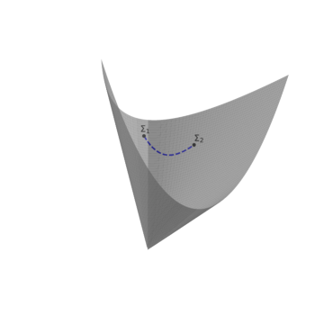
Figure 2.2: Open cone of $\mathbb{P}^{2}$. Visualized is the geodesics connecting $\Sigma_{1},\Sigma_{2}\in\mathbb{P}^{2}$ with respect tothe affine-invariant metric $\langle{\mkern 2.0mu\cdot\mkern 2.0mu},{\mkern 2.0mu\cdot\mkern 2.0mu}\rangle$ (blue, dashed line). Figure inspired by Horev et al. (2016).

Recently, the affine-invariant metric (8) was compared with the Bures-Wasserstein metric (Han et al., 2021) for many problems relevant to machine learning. The authors of Han et al. (2021) found that the affine-invariant metric shows better results for the minimization of $f(\Sigma)=-\log\det(\Sigma)$ due to a lower condition number of the Hessian. Since this function plays a central role in the REML log-likelihood, we chose the affine-invariant metric.

The retraction which is commonly associated with $\mathbb{P}^{d}$ under the Riemannian metric (8) is the exponential map (Jeuris et al., 2012, Hosseini and Sra, 2020a) and given by

$$R_{\Sigma}(\xi)=\Sigma\exp(\Sigma^{-1}\xi).$$ (9)

The associated vector transport is given by (Jeuris et al., 2012, Hosseini and Sra, 2015)

$$\mathscr{T}^{\Sigma}_{\eta}(\xi)=\Sigma^{\frac{1}{2}}\exp\left(\frac{1}{2}\Sigma^{-\frac{1}{2}}\eta\Sigma^{-\frac{1}{2}}\right)\Sigma^{-\frac{1}{2}}\eta\Sigma^{-\frac{1}{2}}\exp\left(\frac{1}{2}\Sigma^{-\frac{1}{2}}\eta\Sigma^{-\frac{1}{2}}\right)\Sigma^{\frac{1}{2}}.$$ (10)

However, usually the identity mapping is preferred for $\mathbb{P}^{d}$ due to the high computational effort of (10). Since the set of positive definite matrices is an open set with the same tangent space at every point (although a varying inner product), the identity map can be deemed appropriate for the vector transport if step sizes do not become too large.

The Riemannian gradient with respect to the inner product (8) is given by (Hosseini and Sra, 2020a, Jeuris et al., 2012)

$$\operatorname{grad}f(\Sigma)=\Sigma\left(\operatorname{grad}^{sym}\bar{f}(\Sigma)\right)\Sigma=\frac{1}{2}\Sigma\left(\operatorname{grad}^{e}\bar{f}(\Sigma)+\left(\operatorname{grad}^{e}\bar{f}(\Sigma)\right)^{T}\right)\Sigma,$$ (11)

where $\operatorname{grad}^{e}\bar{f}$ denotes the classical Euclidean gradient of the smooth extension $\bar{f}$ to the set of real matrices $\mathbb{R}^{d\times d}$ with the Euclidean metric $\langle A,B\rangle=\operatorname{tr}(A^{T}B)$ for $A,B\in\mathbb{R}^{d\times d}$.

Further, the Riemannian Hessian can be found by the Riemannian metric with respect to the inner product (8). It is given by (Jeuris et al., 2012, Sembach et al., 2021)

$$\operatorname{Hess}f(\Sigma)[\xi] =\nabla_{\xi}^{pd}\operatorname{grad}f(\Sigma)=\operatorname{D}\left(\operatorname{grad}f(\Sigma)\right)[\xi]-\frac{1}{2}\left(\xi\Sigma^{-1}\operatorname{grad}f(\Sigma)+\operatorname{grad}f(\Sigma)\Sigma^{-1}\xi\right),$$ (12)

where $\xi\in\mathbb{S}^{d}$.

3 Riemannian approach for Linear Mixed Models

Before formulating the problem as a Riemannian optimization problem over the manifold $\mathbb{P}^{q}$, where $G\in\mathbb{P}^{q}$, we take a closer look at the structure of $H=I+ZGZ^{T}$. We note that the random effects design matrices can be decomposed into $K$ blocks, where $K$ is the number of grouping factors, i.e. $Z=(Z^{(1)},\dots,Z^{(K)})$. Here, each of the blocks consists $M_{j}$ levels which are represented in the data, i.e.

$$Z^{(j)}=\left(Z^{(j,1)},\dots,Z^{(j,M_{j})}\right),$$ (13)

where $Z^{(j,l_{j})}\in\mathbb{R}^{n\times q_{j}}$ and $q=\sum\limits_{j=1}^{K}M_{j}q_{j}$, see Bates et al. (2015), Gumedze and Dunne (2011). The $i$-th row, $i=1,\dots,n$, of $Z^{(j)}$ denoted by $\left(Z^{(j)}\right)_{i}$ has possibly nonzero elements in columns $(l_{j}-1)q_{j}+1,\dots,l_{j}q_{j}$ if and only if observation $i$ arises from the $l_{j}$-th level of the $j$-th grouping factor. Thus, the $i$-th row of the random effects design matrix $Z$ has

$$\sum\limits_{j=1}^{K}\left(M_{j}-1\right)q_{j}$$ (14)

structural zeros, i.e. the sparsity increases with the number of levels $M_{j}$ (Bates et al., 2015). Accordingly, the random effects parameter $b$ can be decomposed into $K$ blocks, that is $b=(b^{(1)},\dots,b^{(K)})$ corresponding to variations introduced by $K$ different grouping factors. Each of the $b^{(j)}$ consists of $M_{j}$ identically and independently distributed random variables, i.e.
$b^{(j)}=(b^{(j,1)},\dots,b^{(j,M_{j})})$, where

$$b^{(j,l_{j})}\stackrel{{\scriptstyle iid}}{{\sim}}\mathcal{N}(0,\Psi_{j}),$$ (15)

where $\Psi_{j}\in\mathbb{R}^{q_{j}\times q_{j}}$. Further, we get

$$G=\left(\begin{array}[]{ccc}G_{1}&&\\ &\ddots&\\ &&G_{K}\end{array}\right),\qquad\text{where }G_{j}=\left(\begin{array}[]{ccc}\Psi_{j}&&\\ &\ddots&\\ &&\Psi_{j},\end{array}\right)$$ (22)

by a suitable ordering of the random effects. Thus, we can express the matrix $H$ in (6) as

$$H=I+ZGZ^{T}=I+\sum\limits_{j=1}^{K}Z^{(j)}G_{j}{Z^{(j)}}^{T}=I+\sum\limits_{j=1}^{K}\sum\limits_{l_{j}=1}^{M_{j}}Z^{(j,l_{j})}\Psi_{j}{Z^{(j,l_{j})}}^{T},$$ (23)

that is $H$ can be expressed by the unknown positive definite matrices $\Psi_{j}$ of the smaller dimensions $q_{j}$. We use this expression of the matrix $H$ for our formulation of the Riemannian optimization problem.

Riemannian formulation.

We consider the residual log-likelihood as presented in (6). The parameters of interest are the residual variance $\sigma^{2}$ and the random effects covariance matrix $G$ which can be expressed via the matrix $\Psi_{j}$ of lower dimension. For the residual variance, we introduce a variable $\eta\in\mathbb{R}$ and set

$$\eta=\log(\sigma^{2}).$$

Further, we use the derived relationship (23) between the covariance matrix $H$ and the matrices $\Psi_{j}$ and rewrite the REML log-likelihood (6) as

$$l_{R}(\theta)=-\frac{1}{2}\left((n-p)\log(2\pi)+(n-p)\eta+\log\det(H)+\log\det(X^{T}H^{-1}X)+\frac{y^{T}P(H)y}{\exp(\eta)}\right),$$ (24)

where $\theta=(\eta,\Psi)$ for $\Psi=(\Psi_{1},\dots,\Psi_{K})$ and $H=I+\sum\limits_{j=1}^{K}\sum\limits_{l_{j}=1}^{M_{j}}Z^{(j,l_{j})}\Psi_{j}{Z^{(j,l_{j})}}^{T}$.
The expression $P(H)$ is given by (5). Since the random effects covariance matrix $G$ is assumed to be positive definite, we must require that the matrices $\Psi_{j}\in\mathbb{R}^{q_{j}\times q_{j}}$ are positive definite. Thus, maximizing the REML objective (24) is a Riemannian optimization problem over the manifold

$${\mathcal{M}}_{LME}=\mathbb{R}\times\left(\operatorname*{\vartimes}_{j=1}^{K}\mathbb{P}^{q_{j}}\right),$$ (25)

where $\mathbb{P}^{q_{j}}$ is the manifold of positive definite matrices of dimension $q_{j}$ with the Riemannian metric (8). The Riemannian optimization problem is summarized in the following.

Optimization problem:
Let $\theta=(\eta,\Psi)$ with $\Psi=(\Psi_{1},\dots,\Psi_{K})$, $\Psi_{j}\succ 0$, $\Psi_{j}\in\mathbb{R}^{q_{j}\times q_{j}}$. For given $X\in\mathbb{R}^{n\times p}$, $Z=(Z^{(1)},\dots,Z^{(K)})\in\mathbb{R}^{n\times q}$ with $Z^{(j)}=(Z^{(j,1)},\dots,Z^{(j,M_{j})})$, $Z^{(j,l_{j})}\in\mathbb{R}^{n\times q_{j}}$ and $y\in\mathbb{R}^{n}$, we consider the Riemannian optimization problem $\displaystyle\min_{\theta\in{\mathcal{M}}_{LME}}L_{R}(\theta)=(n-p)\eta+\log\det(H)+\log\det(X^{T}H^{-1}X)+\frac{y^{T}P(H)y}{\exp(\eta)},$ (26) where $\displaystyle H=I+\sum\limits_{j=1}^{K}\sum\limits_{l_{j}=1}^{M_{j}}Z^{(j,l_{j})}\Psi_{j}{Z^{(j,l_{j})}}^{T},\quad P(H)=H^{-1}-H^{-1}X(X^{T}H^{-1}X)^{-1}X^{T}H^{-1}$ and $\displaystyle{\mathcal{M}}_{LME}=\mathbb{R}\times\left(\operatorname*{\vartimes}_{j=1}^{K}\mathbb{P}^{q_{j}}\right).$

Analogously to the profiled approach in the lme4 package (Douglas Bates, ), we minimize minus twice the function $l_{R}$ in our approach, where $l_{R}$ is as in (6). Further, we drop the term $(n-p)\log(2\pi)$ as it does not affect the optimization.

Riemannian tools for Optimization.

The objective function (26) is a smooth function over the product manifold (25) consisting of the real scalars $\mathbb{R}$ and the $K$ manifolds of positive definite matrices denoted by $\mathbb{P}^{q_{j}}$. We get the tangent space $T_{\theta}{\mathcal{M}}_{LME}$ of the manifold product manifold (25) as the composition of the single tangent spaces, that is

$$T_{\theta}{\mathcal{M}}_{LME}=\mathbb{R}\times\left(\operatorname*{\vartimes}_{j=1}^{K}\mathbb{S}^{q_{j}}\right),$$ (27)

where $\mathbb{S}^{q_{j}}$ denotes the set of symmetric matrices of dimension $q_{j}$.

The inner product $\langle{\mkern 2.0mu\cdot\mkern 2.0mu},{\mkern 2.0mu\cdot\mkern 2.0mu}\rangle_{\theta}$ on $T_{\theta}{\mathcal{M}}_{LME}$ on the product manifold can be constructed by summing the respective metrics, i.e.

$$\langle\xi,\chi\rangle_{\theta}=\xi_{\eta}\chi_{\eta}+\sum\limits_{j=1}^{K}\operatorname{tr}(\Psi_{j}^{-1}\xi_{\Psi_{j}}\Psi_{j}^{-1}\chi_{\Psi_{j}}),$$ (28)

where $\theta=(\eta,\Psi)\in{\mathcal{M}}_{LME}$, $\Psi=(\Psi_{1},\dots,\Psi_{K})$, $\xi_{\theta}=(\xi_{\eta},\xi_{\Psi}),\chi_{\theta}=(\chi_{\eta},\chi_{\Psi})\in T_{\theta}{\mathcal{M}}$ with $\xi_{\Psi}=(\xi_{\Psi_{1}},\dots,\xi_{\Psi_{K}})$, $\chi_{\Psi}=(\chi_{\Psi_{1}},\dots,\chi_{\Psi_{K}})$, $\xi_{\Psi_{j}},\chi_{\Psi_{j}}\in\mathbb{S}^{q_{j}}$, where we used (8).

Accordingly, the retraction associated with the product manifold (25) and the inner product (28) reads

$$R_{\theta}(\xi_{\theta})=\left(\begin{array}[]{c}\eta+\xi_{\eta}\\ \Psi_{1}\exp\left(\Psi_{1}^{-1}\xi_{\Psi_{1}}\right)\\ \vdots\\ \Psi_{K}\exp\left(\Psi_{K}^{-1}\xi_{\Psi_{K}}\right)\end{array}\right),$$ (33)

where $\theta\in{\mathcal{M}}_{LME}$ and $\xi_{\theta}\in T_{\theta}{\mathcal{M}}_{LME}$ as above, see (9).

In the following, we derive expressions for the Riemannian gradient and the Riemannian Hessian of the problem (26). These contribute to a deeper understanding of the underlying geometry of the optimization problem and allow for higher-order Riemannian optimizers in order to solve the optimization problem (26).

Riemannian gradient and Hessian for Linear Mixed Models.

We specify the Riemannian gradient for the problem (26) based on the inner product (28).

Theorem 2

For $\theta\in{\mathcal{M}}_{LME}$, the Riemannian gradient $\operatorname{grad}L_{R}(\theta)\in T_{\theta}{\mathcal{M}}_{LME}$ of problem (26) is given by

$$\operatorname{grad}L_{R}(\theta)=\left(\begin{array}[]{c}\chi_{\eta}\\ \chi_{\Psi}\end{array}\right),$$ (36)

where $\chi_{\Psi}=(\chi_{\Psi_{1}},\dots,\chi_{\Psi_{K}})$ and

$$\chi_{\eta}=(n-p)-\frac{y^{T}P(H)y}{\exp(\eta)},\qquad\chi_{\Psi_{j}}=\Psi_{j}\sum\limits_{l_{j}=1}^{M_{j}}{Z^{(j,l_{j})}}^{T}\operatorname{grad^{e}}_{H}L_{R}(\theta)Z^{(j,l_{j})}\Psi_{j}$$

with

$$\operatorname{grad^{e}}_{H}L_{R}(\theta)=P(H)+\frac{1}{\exp(\eta)}\operatorname{grad^{e}}_{H}(y^{T}P(H)y),$$ (37)

where

$$\operatorname{grad^{e}}_{H}(y^{T}P(H)y) =\bigg{(}-H^{-1}yy^{T}H^{-1}+H^{-1}yv_{1}^{T}H^{-1}+H^{-1}v_{1}y^{T}H^{-1}$$

$$\qquad\qquad-H^{-1}X(X^{T}H^{-1}X^{T})^{-1}X^{T}v_{2}v_{2}^{T}X(X^{T}H^{-1}X^{T})^{-1}X^{T}H^{-1}\bigg{)},$$ (38)

and $v_{1}=X(X^{T}H^{-1}X)^{-1}X^{T}H^{-1}y$, $v_{2}=H^{-1}y$, $P(H)$ as in (5).

Proof. The proof can be found in Appendix A. $\square$

Analogously to unconstrained Euclidean optimization theory, Riemannian optimizers usually benefit from second-order information as they potentially give quadratic local convergence. Thus, besides deriving the Riemannian gradient for linear mixed models in Theorem 2, we present an expression for the Riemannian Hessian of the objective (26) in the following.

Theorem 3

Let $\theta\in{\mathcal{M}}_{LME}$ and $\xi_{\theta}\in T_{\theta}{\mathcal{M}}_{LME}$, $\xi_{\theta}=\left(\xi_{\eta},\xi_{\Psi}\right)$ with $\xi_{\Psi}=\left(\xi_{\Psi_{1}},\dots,\xi_{\Psi_{K}}\right)$. The Riemannian Hessian of problem (26) is given by

$$\operatorname{Hess}L_{R}(\theta)[\xi_{\theta}]=\left(\begin{array}[]{c}\zeta_{\eta}\\ \zeta_{\Psi}\end{array}\right)\in T_{\theta}{\mathcal{M}}_{LME},$$

where

$$\zeta_{\eta} =\frac{1}{\exp(\eta)}\bigg{(}\xi_{\eta}y^{T}P(H)y-\sum\limits_{j=1}^{K}y^{T}\bigg{(}h_{1}\left(\sum\limits_{l_{j}=1}^{M_{j}}Z^{(j,l_{j})}\xi_{\Psi_{j}}{Z^{(j,l_{j})}}^{T}\right)$$

$$\qquad\qquad\qquad\qquad\qquad\qquad\qquad\qquad\qquad\qquad\qquad+h_{2}\left(\sum\limits_{l_{j}=1}^{M_{j}}Z^{(j,l_{j})}\xi_{\Psi_{j}}{Z^{(j,l_{j})}}^{T}\right)\bigg{)}y\bigg{)},$$

and $\zeta_{\Psi}=(\zeta_{\Psi_{1}},\dots,\zeta_{\Psi_{K}})$ with

$$\zeta_{\Psi_{j}} =\Psi_{j}\bigg{(}\sum\limits_{r=1}^{K}\sum\limits_{l_{j}=1}^{M_{j}}{Z^{(j,l_{j})}}^{T}\operatorname{D}_{H}\left(\operatorname{grad^{e}}_{H}L_{R}(\theta)\right)[\sum\limits_{l_{r}=1}^{M_{r}}Z^{(r,l_{r})}\xi_{\Psi_{r}}{Z^{(r,l_{r})}}^{T}]Z^{(j,l_{j})}$$

$$\qquad\qquad\qquad\qquad\qquad\qquad\qquad\quad-\frac{\xi_{\eta}}{\exp(\eta)}\sum\limits_{l_{j}=1}^{M_{j}}{Z^{(j,l_{j})}}^{T}\operatorname{grad^{e}}_{H}(y^{T}P(H)y)Z^{(j,l_{j})}\bigg{)}\Psi_{j}$$

$$\qquad\qquad\qquad+\frac{1}{2}\bigg{(}\xi_{\Psi_{j}}\sum\limits_{l_{j}=1}^{M_{j}}{Z^{(j,l_{j})}}^{T}\operatorname{grad^{e}}_{H}L_{R}(\theta)Z^{(j,l_{j})}\Psi_{j}$$

$$\qquad\qquad\qquad\qquad\qquad\qquad\qquad\qquad\qquad+\Psi_{j}\sum\limits_{l_{j}=1}^{M_{j}}{Z^{(j,l_{j})}}^{T}\operatorname{grad^{e}}_{H}L_{R}(\theta)Z^{(j,l_{j})}\xi_{\Psi_{j}}\bigg{)}$$

Here,

$$\operatorname{D}_{H}\left(\operatorname{grad^{e}}_{H}L_{R}(\theta)\right)[\xi]=h_{1}(\xi)+h_{2}(\xi)+\frac{1}{\exp(\eta)}(h_{3}(\xi)-h_{4}(\xi)),$$

where

$$h_{1}(\xi) =-H^{-1}\xi H^{-1}$$ (39)

$$h_{2}(\xi) =H^{-1}\xi H^{-1}X(X^{T}H^{-1}X)^{-1}X^{T}H^{-1}+H^{-1}X(X^{T}H^{-1}X)^{-1}X^{T}H^{-1}\xi H^{-1}$$

$$\qquad\qquad-H^{-1}X(X^{T}H^{-1}X)^{-1}X^{T}H^{-1}\xi H^{-1}X(X^{T}H^{-1}X)^{-1}X^{T}H^{-1}$$ (40)

$$h_{3}(\xi) =H^{-1}\xi H^{-1}yy^{T}H^{-1}+H^{-1}yy^{T}H^{-1}\xi H^{-1}$$ (41)

$$h_{4}(\xi) =-\left(h_{1}(\xi)+h_{2}(\xi)\right)yy^{T}H^{-1}X(X^{T}H^{-1}X)^{-1}H^{-1}+H^{-1}yy^{T}h_{2}(\xi)$$

$$+\bigg{(}-\left(h_{1}(\xi)+h_{2}(\xi)\right)yy^{T}H^{-1}X(X^{T}H^{-1}X)^{-1}H^{-1}+H^{-1}yy^{T}h_{2}(\xi)\bigg{)}^{T}.$$ (42)

The expressions $\operatorname{grad^{e}}_{H}L_{R}(\theta)$, $\operatorname{grad^{e}}_{H}(y^{T}P(H)y)$ are given by (37) and (38), respectively.

Proof. The proof can be found in Appendix A. $\square$

With the Riemannian approach introduced in this paper, we formulate the objective as a function of both $\sigma^{2}$ and $G$, that is we estimate the residual variance and the random effects covariance matrix simultaneously. This is in contrast to maximizing the profiled log-likelihood as proposed in Bates et al. (2015) and Demidenko (2004). The approach presented here can be easily transferred to optimizing the profiled log-likelihood by substituting $\eta$ by $\hat{\eta}=\log(\hat{\sigma}(G))$, where $\hat{\sigma}(G)$ is the maximum likelihood estimator for fixed $G$.

4 Numerical Experiments

We tested the introduced Riemannian approach on simulated data sets. For this, we compare Riemannian optimization algorithms with the lme4 library (Bates et al., 2015).

Simulation design.

We created data sets with $2$ grouping variables in a crossed design. We used a balanced design (Demidenko, 2004, Section 2.2.1), that is we assumed that all $n$ observations are distributed equally among the $M_{1}$, $M_{2}$ levels of the two grouping factors. To generate the data sets, we followed a similar approach as suggested in DeBruine and Barr (2021). We created $n=1000$ observations for our simulation design. For the fixed effects, we considered one continuous fixed effect and a fixed intercept, thus $p=2$. The fixed effects parameter was set to $\beta=(1,2)^{T}$ for all experiments. For the variance parameters, we set the residual variance for all experiments equal to $\sigma^{2}=0.1$ and created $n=1000$ realizations of a Gaussian distribution with zero mean and variance $\sigma^{2}$ to get realizations of the residual error $\varepsilon$, see (1). To incorporate the random effects in the created data sets, we created $M_{1}$, $M_{2}$ categorical variables reflecting the levels of the two grouping factors. We set the number of levels for the grouping factors equal to $M_{1}=15$ and $M_{2}=10$, respectively. These were then used to build the random effects design matrix $Z$. The numerical tests were conducted for different structures in the grouping variable specific covariance matrices $\Psi_{1}$, $\Psi_{2}$ ($G_{1}$, $G_{2}$). We generated realizations of the random effects parameter ${b=(b^{(1)},b^{(2)})}$ with a Gaussian distribution with zero mean and the covariance matrix ${G=\operatorname{diag}(G_{1},G_{2})}$ according to (15).

With these choices, we created the response vector $y\in\mathbb{R}^{n}$ according to the linear mixed model (1), that is

$$y=X\beta+Zb+\varepsilon.$$

We created $100$ data sets reflecting the same linear mixed model structure with the described simulation approach. We recall that for testing different optimizers, only the variables $y,X$ and $Z$ are available and we do not know the fixed effects parameter $\beta$ or the random effects parameter $b$.

Algorithmic Considerations.

When considering the objective (26) for Riemannian optimization, we observe that we need to evaluate $H\in\mathbb{R}^{n\times n}$ in every iteration as well as terms involving its inverse $H^{-1}$. Since the number of observations $n$ is usually large in applications, precaution is required that the matrix $H$ as well as terms involving its inverse $H^{-1}$ are implemented efficiently. The matrix $H^{t}$ at iteration $t$, $t=0,1,2,\dots$ reads

$$H^{t}=I+Z(G^{t})Z^{T}=I+\sum\limits_{j=1}^{K}Z^{(j)}(G_{j})^{t}{Z^{(j)}}^{T},$$

where

$$G_{j}^{t}=\left(\begin{array}[]{ccc}\Psi_{j}^{t}&&\\ &\ddots&\\ &&\Psi_{j}^{t}\end{array}\right)$$

is the random effects covariance matrix of the $j$-th grouping factor at iteration $t$ and $\Psi_{j}^{t}\in\mathbb{P}^{q_{j}}$ is the coordinate iterate at iteration $t$, see (22). Recall that the grouping factor specific design matrices $Z^{(j)}$ are sparse. For this reason, we store the matrices ${Z^{(j)}}^{T}\in\mathbb{R}^{M_{j}q_{j}\times n}$ in a compressed sparse column (csc) format Chen et al. (2008). Further, each column of ${Z^{(j)}}^{T}$ consists of $\left(M_{j}-1\right)q_{j}$ structural zeros, see (14). Thus, by construction of the matrix $G_{j}^{t}$, the positions of structural zeros in $Z^{(j)}(G_{j}^{t}){Z^{(j)}}^{T}$ are the same for all iterations $t$. This means that only the potential nonzero elements in the matrix $H$ need to be updated in every iteration which is exploited in the implementation used for the numerical results presented. Further, we need to compute factors involving the matrix inverse $({H^{t}})^{-1}$ in every iteration $t$. For this, we use the CHOLMOD approach (Virtanen et al., 2020, Chen et al., 2008) which exploits the sparsity pattern of $ZGZ^{T}$ for the Cholesky decomposition (Bates et al., 2015).

Choice of Optimizers.

Equipped with the Riemannian tools and the derived formulas for the Riemannian gradient and the Hessian in Theorem 2 and Theorem 3, respectively, we used higher-order Riemannian optimization algorithms to test our approach. Due to their fast local convergence close to an optimum, we applied a Riemannian Newton trust-region method (Algorithm 2) and a Riemannian nonlinear conjugate gradient method (Algorithm 1) for the problem of variance estimation in linear mixed models as presented in (26). For the latter, we used the toolbox pymanopt Townsend et al. (2016). For the quadratic subproblem in the Riemannian Newton trust-region algorithm (Algorithm 2), we used the truncated conjugate gradient (tCG) method Steihaug (1983) as a solver. We did not use a preconditioner for the tCG method since we observed very small numbers of inner iterations in the quadratic subproblem during the conduction of the experiments. The initial trust-region radius was set to a default value at $\Delta_{0}=1$ and the hyperparameters of the R-NTR algorithm were set to $\rho^{\prime}=0.1$, $\omega_{1}=1e-3$, $\omega_{2}=0.99$, $\alpha_{1}=0.25$ and $\alpha_{2}=3.5$ according to the suggestions in Gould et al. (2005) .

Input: objective $f$, vector transport $\mathscr{T}$ with associated retraction $R$, initial iterate $\theta^{0}\in{\mathcal{M}}$

Output: sequence of parameters $\{\theta^{t}\}$

1 Set $\eta^{0}=-\operatorname{grad}f(\theta^{0})$

2 for $t=0,1,\dots$ do

3       Compute a suitable step size $\alpha^{t}$ and set

$$\theta^{t+1}=R_{\theta^{t}}(\alpha^{t}\eta^{t});$$

4       Compute $\beta^{t+1}$ and set

$$\eta^{t+1}=-\operatorname{grad}f(\theta^{t+1})+\beta^{t+1}\mathscr{T}_{\alpha^{t}\eta^{t}}(\eta^{t}).$$

5 end for

Algorithm 1 Riemannian (nonlinear) conjugate gradients method (Absil et al., 2008, p. 182)

Input: objective $f$ with linear operator $H$, retraction $R$, initial iterate $\theta^{0}\in{\mathcal{M}}$, initial TR-radius $\Delta_{0}$, maximal TR-radius $\bar{\Delta}$, rejection threshold $\rho^{\prime}\in[0,1/4)$, acceptance parameters $0\leq\omega_{1}\leq\omega_{2}\leq 1,\tau_{1}<1,\tau_{2}>1$

Output: sequence of parameters $\{\theta^{t}\}$

1 for $t=0,1,2,\dots$ do

2       Obtain $s^{t}$ by (approximately) solving the TR-subproblem

$$\min_{s\in T_{\theta^{t}}{\mathcal{M}}}\hat{m}_{\theta^{t}}(s)=f(\theta^{t})+\langle\operatorname{grad}f(\theta^{t}),s\rangle_{\theta^{t}}+\frac{1}{2}\langle H_{t}[s],s\rangle_{\theta^{t}}\quad\text{ s.t. }\langle s,s\rangle_{\theta^{t}}\leq\Delta_{t}^{2};$$

3       Evaluate $\rho_{t}=\frac{f(\theta^{t})-f(R_{\theta^{t}}(s^{t}))}{\hat{m}_{\theta^{t}}(0_{\theta^{t}})-\hat{m}_{\theta^{t}}(s^{t})}$

4       if $\rho_{t}<\omega_{1}$ then

5             $\Delta_{t+1}=\alpha_{1}\Delta_{t}$;

6      else if $\rho_{t}>\omega_{2}$ and $\lVert s^{t}\rVert_{\theta^{t}}=\Delta_{t}$ then

7             $\Delta_{t+1}=\min(\alpha_{2}\Delta_{t},\bar{\Delta})$;

8      else

9             $\Delta_{t+1}=\Delta_{t}$;

10       if $\rho_{t}>\rho^{\prime}$ then

11             $\theta^{t+1}=R_{\theta^{t}}(s^{t})$;

12      else

13             $\theta^{t+1}=\theta^{t}$

14       set $t=t+1$;

15 end for

Algorithm 2 Riemannian trust-region method (Absil et al., 2008, p. 142)

Due to the popularity of the lme4 package (Douglas Bates, ), we compared the established Riemannian optimization approach for REML estimation with the approach implemented in the lme4 package. For this, we used the default optimizers in the lme4 package, the BOBYQA and the Nelder Mead method (Bates et al., 2015).

We initialized the random effects covariance matrices $\Psi_{j}^{0}$ by the identity matrix and the residual variance $(\sigma^{2})^{0}$ by its ML estimator (see Gumedze and Dunne (2011), Bates (2011)), these are the default initializations in the lme4 package (Douglas Bates, ). We stopped all methods when either the number of iterations exceeded $1000$, when the relative difference in the objective between two subsequent iterations fell below $10^{-5}$ (for R-NTR only if we did not reject the tentative direction returned by tCG) or when the step length fell below $10^{-7}$. While the optimizers used in lme4 are derivative-free methods, the aforementioned Riemannian optimizers compute a gradient in each iteration. Thus, we added another stopping criterion for the Riemannian optimizers, that is when the Riemannian norm of the gradient, $\lVert\operatorname{grad}L_{R}(\theta)\rVert_{\theta}$, fell below $10^{-3}$.

All experiments were conducted in Python 3.8 on an Intel Xeon E3-1200 at 1.90 GHz with 8 cores and 16GB RAM.

Numerical Results.

We present results for two simulation settings. The first setting is a crossed random effects design with two random intercepts which results in the dimensions $q_{1}=q_{2}=1$. Thus, the structure of the grouping effect specific random effects covariance matrix is given by

$$\Psi_{j}=\left(\tau_{j}^{2}\right),$$ (43)

where $\tau_{j}$ is the standard deviation of the $j$-th random effect. The random effects variance parameters were chosen as $\tau_{1}=1.2$ and $\tau_{2}=0.9$ and the residual variance as $\sigma^{2}=0.1$. As outlined before, the values were initialized at $\tau_{1}^{0}=\tau_{2}^{0}=1$. Table 4.1 shows a summary of the optimization results of $100$ simulation runs, i.e. of $100$ generated data sets following the specified distribution. We observe that the Riemannian optimizers (R-NTR, R-CG) together with the lme4 approach with the Nelder Mead optimizer (NELDERMEAD) show the best results in terms of the objective value $L_{R}$ although the deviation from the true objective (av. deviation $L_{R}$) is slightly higher than for the BOBYQA optimizer. In terms of the mean squared errors of the $\tau_{1}$, $\tau_{2}$ parameters (MSE $\tau_{1}$, $\tau_{2}$), we observe that both the Riemannian Newton trust-region algorithm as well as the Nelder Mead optimizer show comparable results, whereas the BOBYQA optimizer shows a higher error. In contrast, for the residual standard deviation $\sigma$, BOBYQA shows the lowest mean squared errors which is slightly below the mean squared error of the other methods. The Riemannian Newton trust-region algorithm converged in comparably few iterations, underlining the fast local convergence of the method. However, the Riemannian optimizers show much higher overall runtimes compared to the lme4 approach with BOBYQA or Nelder Mead. This can be mainly led back to the high computational costs of evaluating the Riemannian gradient (and the Riemannian Hessian for R-NTR) in every iteration, whereas the BOBYQA and the Nelder Mead algorithms are derivative-free and have very low per-iteration costs for parameters of low dimensions (here: dimension $2$) Bates et al. (2015).

Table 4.1: Simulation results for two random intercepts with ${\tau_{1}=1.2}$, ${\tau_{2}=0.9}$, ${\sigma^{2}=0.1}$ and $M_{1}=15$, $M_{2}=10$.

	R-NTR	R-CG	BOBYQA	NELDERMEAD
av. number of iterations	12.01	55.17	61.43	36.16
av. runtime (s)	6.47	24.76	0.05	0.04
av. $L_{R}$	-1.5474	-1.5474	-1.4659	-1.5474
av. deviation $L_{R}$	2.2505	2.2505	2.0669	2.2505
MSE $\tau_{1}$	0.0427	0.0427	0.2336	0.0434
MSE $\tau_{2}$	0.0426	0.0426	0.1508	0.0425
MSE $\sigma$	0.0468	0.0468	0.0446	0.0468

The appropriateness of Riemannian optimizers for linear mixed models was tested on a second setting, where a random slope for the second grouping factor was added, i.e. $q_{2}=2$. The structure of the covariance matrix $G_{1}$ belonging to the first grouping factor ${\mathcal{B}}_{1}$ is the same as before and given by (43), whereas the structure of the covariance matrix belonging to the second grouping factor is given by

$$\Psi_{2}=\left(\begin{array}[]{cc}\tau_{{2}_{1}}^{2}&\rho_{2}\tau_{{2}_{1}}\tau_{{2}_{2}}\\ \rho_{2}\tau_{{2}_{1}}\tau_{{2}_{2}}&\tau_{{2}_{2}}^{2}\end{array}\right)$$ (46)

For the simulation, we set $\tau_{1}=\tau_{{2}_{1}}=\tau_{{2}_{2}}=1$ and $\rho_{2}=0.1$. We used the same residual variance as above, $\sigma^{2}=0.1$, to create $100$ data sets for the simulation. The simulation results for this setting are summarized in Table 4.2.

Table 4.2: Simulation results for two random effects $b^{(1)}\in\mathbb{R}$, $b^{(2)}\in\mathbb{R}^{2}$ with $\tau_{1}=\tau_{{2}_{1}}=\tau_{{2}_{2}}=1$, $\rho_{2}=0.1$, ${\sigma^{2}=0.1}$ and $M_{1}=15$, $M_{2}=10$.

	R-NTR	R-CG	BOBYQA	NELDERMEAD
av. number of iterations	21.55	30.6	79.88	83.28
av. runtime (s)	11.79	14.38	0.06	0.06
av. $L_{R}$	-1.5378	-1.5381	-1.5305	-1.5393
av. deviation $L_{R}$	2.2922	2.2933	2.2711	2.2969
MSE $\tau_{1}$	0.0336	0.0341	0.0847	0.0342
MSE $\tau_{{2}_{1}}$	0.0542	0.0493	0.3093	0.3860
MSE $\tau_{{2}_{2}}$	0.2669	0.3040	0.8990	0.6209
MSE $\rho_{2}$	0.000114	0.000056	0.009555	0.00862
MSE $\sigma$	0.0466	0.0466	0.0464	0.0467

When comparing the mean squared errors for the random effects covariance matrix, we observe that the Riemannian optimizers show much better results which is visible for the second random effect in particular (MSE $\tau_{{2}_{1}}$, $\tau_{{2}_{2}}$). Those are remarkably low compared to the lme4 optimizers. We also attain a much lower mean squared error for the correlation $\rho_{2}$ with the Riemannian optimizers. We observe that both Riemannian optimizers converge much faster than the lme4 optimizers in terms of number of iterations whereas the runtimes are much higher which we also noticed for the first setting. The improved model quality of the Riemannian optimizers is remarkable as we could improve the MSE with a factor up to $8$.

5 Conclusion

We took a look at variance parameter estimation from a geometric optimization perspective. For this, we introduced a novel Riemannian optimization approach for maximizing the REML log-likelihood of linear mixed models. Based on the introduced formulation, we derived explicit formulas for both the Riemannian gradient and the Riemannian Hessian which can be used to build efficient algorithms posed on Riemannian manifolds. We showed that with the Riemannian optimizers tested we received a much better quality of the parameter estimates compared to existing methods. The effect was stronger for a more complex covariance design of the random effects. These promising results give rise to further investigations for more advanced mixed models, e.g., for more complex random effects designs (e.g. more grouping factors, higher number of random slopes) or generalized mixed models that are potentially harder to fit with existing optimizers.

Appendix A Proofs of Theorem 2 and Theorem 3

Proof of Theorem 2.
The Riemannian gradient for linear mixed models is given by the Riemannian gradient of the single components, that is

$$\operatorname{grad}L_{R}(\theta)=\left(\begin{array}[]{c}\operatorname{grad}_{\eta}L_{R}(\theta)\\ \operatorname{grad}_{\Psi_{1}}L_{R}(\theta)\\ \vdots\\ \operatorname{grad}_{\Psi_{K}}L_{R}(\theta)\end{array}\right),$$

where $\operatorname{grad}_{\eta}L_{R}(\theta)\in\mathbb{R}$, $\operatorname{grad}_{\Psi_{j}}L_{R}(\theta)\in\mathbb{S}^{q_{j}}$ denotes the gradient with regard to $\eta$ and $\Psi_{j}$, respectively.

We first specify the Euclidean gradient $\operatorname{grad}_{\eta}L_{R}(\theta)$ of $L_{R}$ with respect to $\eta$. Here, the Riemannian gradient is equal to the Euclidean gradient and reads

$$\operatorname{grad}_{\eta}L_{R}(\theta)=(n-p)-\frac{1}{\exp(\eta)}y^{T}P(H)y,$$

yielding the expression for $\chi_{\eta}$.

The Riemannian gradient with respect to $\Psi_{j}$ is given by

$$\operatorname{grad}_{\Psi_{j}}L_{R}(\theta)=\frac{1}{2}\Psi_{j}\left(\operatorname{grad^{e}}_{\Psi_{j}}L_{R}(\theta)+\left(\operatorname{grad^{e}}_{\Psi_{j}}L_{R}(\theta)\right)^{T}\right)\Psi_{j},$$ (47)

where $\operatorname{grad^{e}}_{\Psi_{j}}L_{R}(\theta)$ denotes the Euclidean gradient of the Euclidean smooth extension of $L_{R}(\theta)$ with respect to $\Psi_{j}$, see (11). We specify the Euclidean gradient $\operatorname{grad^{e}}_{\Psi_{j}}$ for all $j=1,\dots,K$ in the following. By the chain rule, we get

$$\operatorname{grad^{e}}_{\Psi_{j}}L_{R}(\theta)=\sum\limits_{l_{j}=1}^{M_{j}}{Z^{(j,l_{j})}}^{T}\operatorname{grad^{e}}_{H}L_{R}(\theta)Z^{(j,l_{j})},$$ (48)

where $\operatorname{grad^{e}}_{H}L_{R}(\theta)$ is the Euclidean gradient of $L_{R}$ with respect to the matrix $H\in\mathbb{R}^{n\times n}$ given by (23). By again applying the chain rule, we obtain

$$\operatorname{grad^{e}}_{H}L_{R}(\theta) =H^{-1}-H^{-1}X(X^{T}H^{-1}X^{T})^{-1}X^{T}H^{-1}+\frac{1}{\exp(\eta)}\left(\operatorname{grad^{e}}_{H}(y^{T}P(H)y)\right).$$ (49)

We define

$$u_{1}(H)\coloneqq y^{T}H^{-1}y,\qquad u_{2}(H)\coloneqq y^{T}H^{-1}X(X^{T}H^{-1}X^{T})^{-1}X^{T}H^{-1}y,$$

hence the last expression in (49) is given by

$$\operatorname{grad^{e}}_{H}(y^{T}P(H)y)=\operatorname{grad^{e}}(u_{1}(H))-\operatorname{grad^{e}}(u_{2}(H)).$$ (50)

With the Leibniz rule, we get

$$\operatorname{grad^{e}}(u_{1}(H)) =-H^{-1}yy^{T}H^{-1}$$

$$\operatorname{grad^{e}}(u_{2}(H)) =-\bigg{(}H^{-1}yv_{1}^{T}H^{-1}+H^{-1}v_{1}y^{T}H^{-1}$$

$$\quad\qquad\qquad-H^{-1}X(X^{T}H^{-1}X^{T})^{-1}X^{T}v_{2}v_{2}^{T}X(X^{T}H^{-1}X^{T})^{-1}X^{T}H^{-1}\bigg{)},$$ (51)

where we have set $v_{1}=X(X^{T}H^{-1}X)^{-1}X^{T}H^{-1}y$ and $v_{2}=H^{-1}y$.
We plug (51) into (50), (49), (48) and use the relationship of the Euclidean and Riemannian gradient given by (47). The symmetry of the Euclidean gradient $\operatorname{grad^{e}}_{\Psi_{j}}$ with respect to $\Psi_{j}$ yields the expression for $\operatorname{grad}_{\Psi_{j}}L_{R}(\theta)$. $\square$

Proof of Theorem 3.
The Riemannian Hessian is given by

$$\operatorname{Hess}L_{R}(\theta)[\xi_{\theta}]=\nabla_{\theta}\operatorname{grad}L_{R}(\theta)=\left(\begin{array}[]{c}\zeta_{\eta}\\ \left(\zeta_{\Psi_{j}}\right)_{j=1,\dots,K}\end{array}\right)=\left(\begin{array}[]{c}\nabla_{\xi_{\eta}}^{e}\operatorname{grad}L_{R}(\theta)\\ \left(\nabla_{\xi_{\Psi_{j}}}^{pd}\operatorname{grad}L_{R}(\theta)\right)_{j=1,\dots,K}\end{array}\right)$$ (56)

where $\nabla^{e}_{\xi_{\eta}}$ denotes the classical Euclidean vector field differentiation along direction $\xi_{\eta}$ and $\nabla_{\xi_{\Psi_{j}}}^{pd}$ denotes the Riemannian connection for positive definite matrices Jeuris et al. (2012).

For the Hessian at position $\eta$ denoted by $\zeta_{\eta}$, we observe that

$$\zeta_{\eta}=\nabla_{\xi_{\eta}}^{e}\operatorname{grad}L_{R}(\theta)=\operatorname{D}_{\eta}\left(\operatorname{grad^{e}}_{\eta}L_{R}(\theta)\right)[\xi_{\eta}]+\sum\limits_{j=1}^{K}\operatorname{D}_{\Psi_{j}}\left(\operatorname{grad^{e}}_{\eta}L_{R}(\theta)\right)[\xi_{\Psi_{j}}].$$

We get

$$\operatorname{D}_{\eta}\left(\operatorname{grad^{e}}_{\eta}L_{R}(\theta)\right)[\xi_{\eta}]=\frac{\xi_{\eta}}{\exp(\eta)}y^{T}P(H)y,$$

and

$$\operatorname{D}_{\Psi_{j}}\left(\operatorname{grad^{e}}_{\eta}L_{R}(\theta)\right)[\xi_{\Psi_{j}}] =-\frac{1}{\exp(\eta)}\operatorname{D}_{\Psi_{j}}(y^{T}P(H)y)[\xi_{\Psi_{j}}]$$

$$=-\frac{1}{\exp(\eta)}\operatorname{D}_{H}(y^{T}P(H)y)[\sum\limits_{l_{j}=1}^{M_{j}}Z^{(j,l_{j})}\xi_{\Psi_{j}}{Z^{(j,l_{j})}}^{T}].$$ (57)

By applying the chain rule on (57), we get the expression for $\zeta_{\eta}$ in Theorem 3.

For the Riemannian Hessian at position $\Psi_{j}$ denoted by $\zeta_{\Psi_{j}}$, using (12), we get

$$\zeta_{\Psi_{j}} =\nabla_{\xi_{\Psi_{j}}}^{pd}\operatorname{grad}L_{R}(\theta)$$

$$=\operatorname{D}_{\theta}(\operatorname{grad}_{\Psi_{j}}L_{R}(\theta))[\xi_{\theta}]-\frac{1}{2}\left(\xi_{\Psi_{j}}{\Psi_{j}}^{-1}\operatorname{grad}_{\Psi_{j}}L_{R}(\theta)+\operatorname{grad}_{\Psi_{j}}L_{R}(\theta){\Psi_{j}}^{-1}\xi_{\Psi_{j}}\right)$$

$$=\operatorname{D}_{\eta}(\operatorname{grad}_{\Psi_{j}}L_{R}(\theta))[\xi_{\eta}]+\sum\limits_{r=1}^{K}\operatorname{D}_{\Psi_{r}}\left(\operatorname{grad}_{\Psi_{j}}L_{R}(\theta)\right)[\xi_{\Psi_{r}}]$$

$$\qquad\qquad\qquad\qquad\qquad-\frac{1}{2}\left(\xi_{\Psi_{j}}{\Psi_{j}}^{-1}\operatorname{grad}_{\Psi_{j}}L_{R}(\theta)+\operatorname{grad}_{\Psi_{j}}L_{R}(\theta){\Psi_{j}}^{-1}\xi_{\Psi_{j}}\right)$$

$$=\operatorname{D}_{\eta}(\operatorname{grad}_{\Psi_{j}}L_{R}(\theta))[\xi_{\eta}]+\Psi_{j}\left(\sum\limits_{r=1}^{K}\operatorname{D}_{\Psi_{r}}\left(\operatorname{grad^{e}}_{\Psi_{j}}L_{R}(\theta)\right)[\xi_{\Psi_{r}}]\right)\Psi_{j}$$

$$\qquad\qquad\qquad\qquad\qquad+\frac{1}{2}\left(\xi_{\Psi_{j}}\operatorname{grad^{e}}_{\Psi_{j}}L_{R}(\theta)\Psi_{j}+\Psi_{j}\operatorname{grad^{e}}_{\Psi_{j}}L_{R}(\theta)\xi_{\Psi_{j}}\right),$$ (58)

where we used (48). For the first term in (58), we get

$$\operatorname{D}_{\eta}(\operatorname{grad}_{\Psi_{j}}L_{R}(\theta))[\xi_{\eta}]=-\frac{\xi_{\eta}}{\exp(\eta)}\Psi_{j}\left(\sum\limits_{l_{j}=1}^{M_{j}}Z^{(j,l_{j})}\operatorname{grad^{e}}_{H}(y^{T}P(H)y){Z^{(j,l_{j})}}^{T}\right)\Psi_{j},$$ (59)

where $\operatorname{grad^{e}}_{H}(y^{T}P(H)y)$ is given by (38).

For the second term in (58), we get

$$\operatorname{D}_{\Psi_{r}}\left(\operatorname{grad^{e}}_{\Psi_{j}}L_{R}(\theta)\right)[\xi_{\Psi_{r}}] =\sum\limits_{l_{j}=1}^{M_{j}}Z^{(j,l_{j})}\operatorname{D}_{\Psi_{r}}\left(\operatorname{grad^{e}}_{H}L_{R}(\theta)\right)[\xi_{\Psi_{r}}]{Z^{(j,l_{j})}}^{T}$$

$$=\sum\limits_{l_{j}=1}^{M_{j}}Z^{(j,l_{j})}\operatorname{D}_{H}\left(\operatorname{grad^{e}}_{H}L_{R}(\theta)\right)[\sum\limits_{l_{r}=1}^{M_{r}}Z^{(r,l_{r})}\xi_{\Psi_{r}}{Z^{(r,l_{r})}}^{T}]{Z^{(j,l_{j})}}^{T}$$ (60)

by the chain rule. After applying the Leibniz rule on (60) several times and rearrangement of terms, we get

$$\operatorname{D}_{H}\left(\operatorname{grad^{e}}_{H}L_{R}(\theta)\right)[\xi]=h_{1}(\xi)+h_{2}(\xi)+\frac{1}{\exp(\eta)}(h_{3}(\xi)-h_{4}(\xi)),$$ (61)

where $h_{1}$, $h_{2}$ as in (39), (40) and $h_{3}$, $h_{4}$ as in (41), (42).

Plugging (61) into (60) and then (60), (59) into (58), we get the expression for $\zeta_{\Psi_{j}}$ in Theorem 3. $\square$

References

- Absil et al. (2008) P.-A. Absil, R. Mahony, and R. Sepulchre. Optimization Algorithms on Matrix Manifolds. Princeton University Press, Princeton, NJ, 2008. ISBN 978-0-691-13298-3.
- Arnaudon et al. (2013) M. Arnaudon, F. Barbaresco, and L. Yang. Riemannian medians and means with applications to radar signal processing. IEEE Journal of Selected Topics in Signal Processing, 7(4):595–604, 2013.
- Bates (2011) D. Bates. Computational methods for mixed models. Vignette for lme4, 2011.
- Bates et al. (2015) D. Bates, M. Mächler, B. Bolker, and S. Walker. Fitting Linear Mixed-Effects Models using lme4. Journal of Statistical Software, 67(1):1–48, 2015. doi: 10.18637/jss.v067.i01. URL https://www.jstatsoft.org/index.php/jss/article/view/v067i01.
- Bhatia (2007) R. Bhatia. Positive Definite Matrices. Princeton Series in Applied Mathematics. Princeton University Press, Princeton, NJ, USA, 2007.
- Boumal (2022) N. Boumal. An introduction to optimization on smooth manifolds. To appear with Cambridge University Press, Apr 2022. URL http://www.nicolasboumal.net/book.
- Chen et al. (2008) Y. Chen, T. A. Davis, W. W. Hager, and S. Rajamanickam. Algorithm 887: Cholmod, supernodal sparse Cholesky factorization and update/downdate. ACM Transactions on Mathematical Software (TOMS), 35(3):1–14, 2008.
- Cherian and Sra (2016) A. Cherian and S. Sra. Positive definite matrices: data representation and applications to computer vision. In Algorithmic advances in Riemannian geometry and applications, pages 93–114. Springer, 2016.
- DeBruine and Barr (2021) L. M. DeBruine and D. J. Barr. Understanding mixed-effects models through data simulation. Advances in Methods and Practices in Psychological Science, 4(1), 2021.
- Demidenko (2004) E. Demidenko. Mixed Models - Theory and Applications. Wiley, New York, 2004. ISBN 978-0-471-60161-6.
- Dempster et al. (1981) A. P. Dempster, D. B. Rubin, and R. K. Tsutakawa. Estimation in covariance components models. Journal of the American Statistical Association, 76(374):341–353, 1981.
- Doran et al. (2007) H. Doran, D. Bates, P. Bliese, and M. Dowling. Estimating the multilevel Rasch model: With the lme4 package. Journal of Statistical software, 20:1–18, 2007.
- (13) B. B. S. W. R. H. B. C. H. S. B. D. F. S. G. G. P. G. J. F. A. B. P. N. K. Douglas Bates, Martin Maechler. lme4: Linear mixed-effects models using ’eigen’ and s4.
- Gould et al. (2005) N. Gould, D. Orban, A. Sartenaer, and P. Toint. Sensitivity of trust-region algorithms to their parameters. 4OR quarterly journal of the Belgian, French and Italian Operations Research Societies, 3:227–241, 2005. doi: 10.1007/s10288-005-0065-y.
- Gueorguieva and Krystal (2004) R. Gueorguieva and J. H. Krystal. Move over ANOVA: progress in analyzing repeated-measures data andits reflection in papers published in the archives of general psychiatry. Archives of general psychiatry, 61(3):310–317, 2004.
- Gumedze and Dunne (2011) F. Gumedze and T. Dunne. Parameter estimation and inference in the linear mixed model. Linear Algebra and its Applications, 435(8):1920–1944, 2011.
- Han et al. (2021) A. Han, B. Mishra, P. Jawanpuria, and J. Gao. On Riemannian Optimization over Positive Definite Matrices with the Bures-Wasserstein Geometry, 2021.
- Horev et al. (2016) I. Horev, F. Yger, and M. Sugiyama. Geometry-aware principal component analysis for symmetric positive definite matrices. Machine Learning, 106(4):493–522, 2016. doi: 10.1007/s10994-016-5605-5. URL https://doi.org/10.1007/s10994-016-5605-5.
- Hosseini and Sra (2015) R. Hosseini and S. Sra. Matrix manifold optimization for Gaussian mixtures. Advances in Neural Information Processing Systems, 28, 2015.
- Hosseini and Sra (2020a) R. Hosseini and S. Sra. An alternative to EM for gaussian mixture models: batch and stochastic riemannian optimization. Math. Program., 181(1):187–223, 2020a.
- Hosseini and Sra (2020b) R. Hosseini and S. Sra. An alternative to EM for Gaussian mixture models: batch and stochastic Riemannian optimization. Mathematical programming, 181(1):187–223, 2020b.
- Hua et al. (2017) X. Hua, Y. Cheng, H. Wang, Y. Qin, Y. Li, and W. Zhang. Matrix CFAR detectors based on symmetrized Kullback–Leibler and total Kullback–Leibler divergences. Digital Signal Processing, 69:106–116, 2017.
- Jeuris et al. (2012) B. Jeuris, R. Vandebril, and B. Vandereycken. A survey and comparison of contemporary algorithms for computing the matrix geometric mean. ETNA, 39:379–402, 2012.
- Lee and Park (2018) T. Lee and F. C. Park. A geometric algorithm for robust multibody inertial parameter identification. IEEE Robotics and Automation Letters, 3(3):2455–2462, 2018.
- Lindstrom and Bates (1988) M. J. Lindstrom and D. M. Bates. Newton–Raphson and EM algorithms for linear mixed-effects models for repeated-measures data. Journal of the American Statistical Association, 83(404):1014–1022, 1988.
- Moakher and Zéraï (2011) M. Moakher and M. Zéraï. The Riemannian geometry of the space of positive-definite matrices and its application to the regularization of positive-definite matrix-valued data. Journal of Mathematical Imaging and Vision, 40(2):171–187, 2011.
- Morales and Nocedal (2000) J. Morales and J. Nocedal. Automatic Preconditioning by Limited Memory Quasi-Newton Updating. SIAM Journal on Optimization, 10:1079–1096, 06 2000.
- Pinheiro and Bates (2006) J. Pinheiro and D. Bates. Mixed-effects models in S and S-PLUS. Springer Science & Business media, 2006.
- Pinheiro et al. (2022) J. Pinheiro, D. Bates, and R Core Team. nlme: Linear and nonlinear mixed effects models. 2022. URL https://CRAN.R-project.org/package=nlme. R package version 3.1-158.
- Sato (2021) H. Sato. Riemannian Optimization and Its Applications. SpringerBriefs in Electrical and Computer Engineering, 2021. doi: 10.1007/978-3-030-62391-3. URL https://doi.org/10.1007/978-3-030-62391-3.
- Sembach et al. (2021) L. Sembach, J. P. Burgard, and V. Schulz. A Riemannian Newton trust-region method for fitting Gaussian mixture models. Statistics and Computing, 32(1), 2021. doi: 10.1007/s11222-021-10071-1. URL https://doi.org/10.1007/s11222-021-10071-1.
- Steihaug (1983) T. Steihaug. The conjugate gradient method and trust regions in large scale optimization. SIAM Journal on Numerical Analysis, 20(3):626–637, 1983. doi: 10.1137/0720042. URL https://doi.org/10.1137/0720042.
- Townsend et al. (2016) J. Townsend, N. Koep, and S. Weichwald. Pymanopt: A python toolbox for optimization on manifolds using automatic differentiation. Journal of Machine Learning Research, 17(137):1–5, 2016. URL http://jmlr.org/papers/v17/16-177.html.
- Vandereycken (2013) B. Vandereycken. Low-rank matrix completion by Riemannian optimization. SIAM Journal on Optimization, 23(2):1214–1236, 2013.
- Virtanen et al. (2020) P. Virtanen, R. Gommers, T. E. Oliphant, M. Haberland, T. Reddy, D. Cournapeau, E. Burovski, P. Peterson, W. Weckesser, J. Bright, S. J. van der Walt, M. Brett, J. Wilson, K. J. Millman, N. Mayorov, A. R. J. Nelson, E. Jones, R. Kern, E. Larson, C. J. Carey, İ. Polat, Y. Feng, E. W. Moore, J. VanderPlas, D. Laxalde, J. Perktold, R. Cimrman, I. Henriksen, E. A. Quintero, C. R. Harris, A. M. Archibald, A. H. Ribeiro, F. Pedregosa, P. van Mulbregt, and SciPy 1.0 Contributors. SciPy 1.0: Fundamental Algorithms for Scientific Computing in Python. Nature Methods, 17:261–272, 2020. doi: 10.1038/s41592-019-0686-2.