Masked Wavelet Representation for Compact Neural Radiance Fields

Abstract

Neural radiance fields (NeRF) have demonstrated the potential of coordinate-based neural representation (neural fields or implicit neural representation) in neural rendering. However, using a multi-layer perceptron (MLP) to represent a 3D scene or object requires enormous computational resources and time. There have been recent studies on how to reduce these computational inefficiencies by using additional data structures, such as grids or trees. Despite the promising performance, the explicit data structure necessitates a substantial amount of memory. In this work, we present a method to reduce the size without compromising the advantages of having additional data structures. In detail, we propose using the wavelet transform on grid-based neural fields. Grid-based neural fields are for fast convergence, and the wavelet transform, whose efficiency has been demonstrated in high-performance standard codecs, is to improve the parameter efficiency of grids. Furthermore, in order to achieve a higher sparsity of grid coefficients while maintaining reconstruction quality, we present a novel trainable masking approach. Experimental results demonstrate that non-spatial grid coefficients, such as wavelet coefficients, are capable of attaining a higher level of sparsity than spatial grid coefficients, resulting in a more compact representation. With our proposed mask and compression pipeline, we achieved state-of-the-art performance within a memory budget of 2 MB. Our code is available at https://github.com/daniel03c1/masked_wavelet_nerf.

1 Introduction

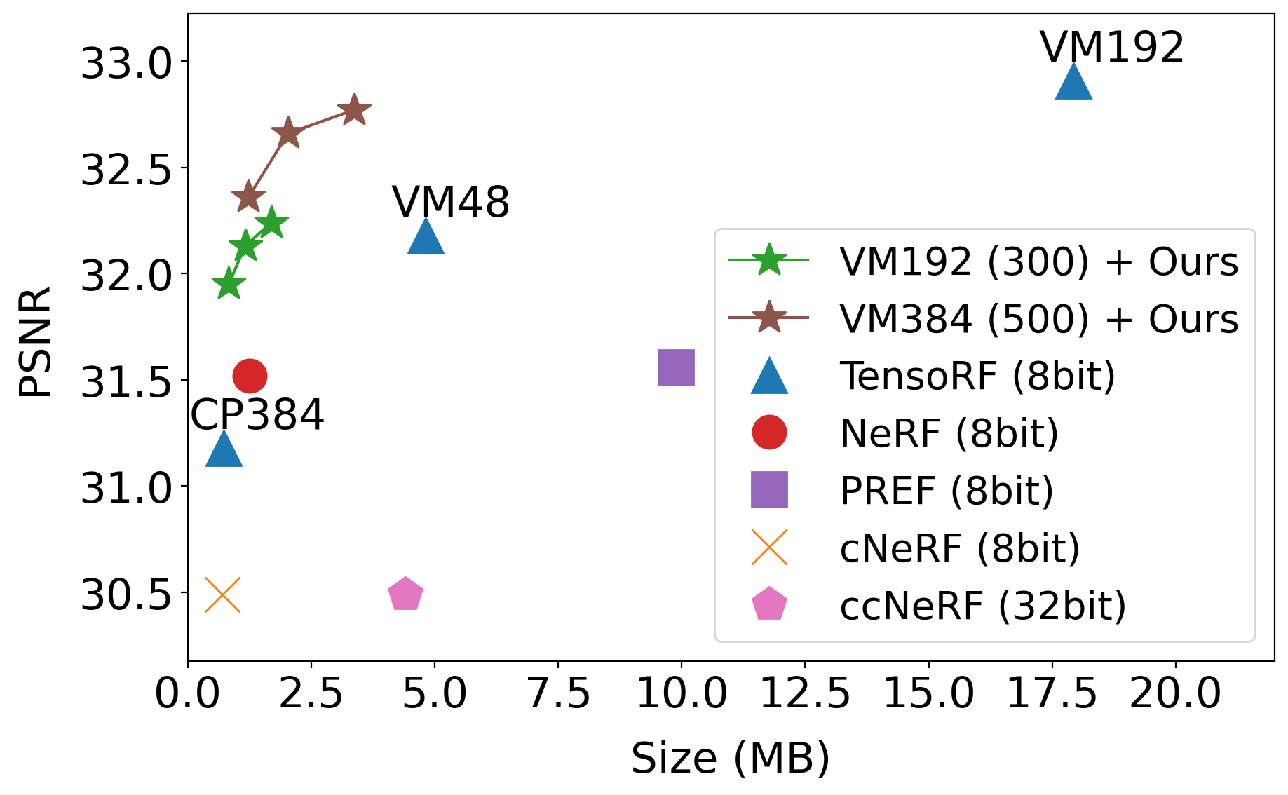
Figure 1: Rate-distortion curves on the NeRF synthetic dataset. The numbers inside parenthesis denote the axis resolution of grids.

Recent advances in coordinate-based neural representation (neural fields or implicit neural representation) have demonstrated remarkable performance in many applications. In particular, neural radiance fields (NeRF) have sparked interest by synthesizing high-quality images from novel viewpoints. It uses a multi-layer perceptron (MLP) with positional encoding to map coordinates to corresponding colors and opacities. Combined with the differentiable volumetric rendering and the neural network’s architectural priors, it has shown great potential to be a new representation paradigm. However, the high computational costs (in both training and inference) have been a significant bottleneck, often taking several days to converge.

Several follow-up studies have been proposed to accelerate training and inference times [33, 14, 41, 11, 45, 16, 5, 9, 32]. To speed up inference, KiloNeRF [33] proposed splitting a 3D scene into thousands of partial scenes, each of which is assigned a tiny, distinct neural network. While achieving impressive speed-up, it requires a massive amount of memory storage. On the other hand, FastNeRF [14] suggested caching and factorizing the NeRF network to reduce computational costs. Meanwhile, meta-learning algorithms [12, 26, 30] have also been applied to accelerate the training time, and they have shown faster convergence with the learned initialization [41, 35]. However, it requires well-organized large-scale datasets and a pre-training process. Furthermore, the rendering costs remain unchanged since they use the same network architecture [41], and meta-learning algorithms often suffer from poor out-of-distribution generalization performance.

Alternatively, there has been a surge of recent interest in incorporating classical data structures, such as grids or trees, into the NeRF framework [22, 13, 50, 24, 39, 40, 34]. Incorporating additional data structures has significantly reduced training and inference time (from days to a few minutes) without compromising reconstruction quality. However, the overall size dramatically increases due to these dense and volumetric structures. In order to reduce the spatial complexity, several methods have been proposed, including pruning areas [50, 38, 34], encodings [24, 39], and tensor decomposition [3, 4, 17].

This paper aims to further improve the spatial complexity while maintaining the rendering quality. Leveraging the decades of research on standard compression algorithms [36, 47, 37], we propose compressing grid-based neural fields using frequency-based transformations. In the frequency domain, a large portion of the coefficients can be discarded without considerably degrading the reconstruction quality, and most standard compression algorithms have exploited frequency domain representations. Thus, we propose using this property on grid-based neural fields to maximize parameter efficiency. Among other alternatives, we employ the discrete wavelet transform (DWT) due to its compactness and ability to efficiently capture both global and local information.

Once we obtain sparse representations via frequency domain representations, we can take advantage of the existing compression techniques. Unlike conventional media data (e.g., image and audio), however, no off-the-shelf compression tools exist that we can leverage without complicated engineering efforts. In addition, since NeRF, or neural rendering networks in general, is a relatively new data format, the characteristics or patterns of their coefficients have not been thoroughly investigated. Thus, we present a compression pipeline for our purposes. To automatically filter out unnecessary coefficients, we propose a trainable binary mask. For each 3D scene, we jointly optimize grid parameters and their corresponding masks. This per-scene optimization strategy can be more optimal than the global quantization table used in standard image compression codecs [44].

To compress sparse grid representations, we first merge masks with wavelet coefficients to zero out coefficients and then apply standard compression algorithms to masked coefficients. We utilize the run-length encoding to encode binary information about which coefficients are non-zero. For further compression, we apply one of the entropy coding algorithms, Huffman encoding [19], to these encoded outputs.

Our method incurs negligible computational costs at test time, requiring only one inverse DWT (IDWT) per grid. After the IDWT, the wavelet grids are transformed into spatial grids, eliminating the need for additional IDWT during rendering. As a result, the computing time and costs (including memory costs) are identical to the original spatial grid-based NeRF.

In summary, our contributions are as follows:

• We propose using wavelet coefficients to improve parameter sparsity and reconstruction quality. Through experiments, we show that the wavelet coefficients can be more compact than the spatial domain coefficients in neural radiance fields.

• We propose a trainable mask that can be applied to any grid-based neural representation. Experimental results demonstrate that our proposed masking method can zero out more than 95% of the total grid parameters while maintaining high reconstruction quality.

• We achieve state-of-the-art performance in novel view synthesis under a memory budget of 2 MB.

2 Related Works

2.1 Neural rendering

Neural radiance fields. NeRF [23] has demonstrated that 3D scenes and objects can be successfully represented using coordinate-based neural representation. NeRF renders a scene by casting a ray per pixel and sampling colors and opacity from points that lie on the ray. However, since this approach relies on the dense, point-wise sampling of color values and opacity, the computational costs are significant.

Due to this inefficiency, there has been considerable interest in improving computational efficiency. A plethora of methods propose to adopt data structures such as trees [50, 46], point clouds [49, 27, 51, 28], and grids [13, 15, 24, 39, 4, 38, 34] to efficiently represent 3D scenes and objects. PlenOctrees [50] use an octree structure for real-time rendering. Despite the reduced rendering costs, the increased size of more than ten times the size of standard MLP-based neural fields, such as NeRF [23], limits their wide application. Point cloud-based approaches [49, 27] reduce the number of points sampled per ray by utilizing the scene geometry of a point cloud. Lastly, a number of studies have demonstrated the efficiency of using grid structures, including vectors, matrices, and tensors, on neural fields [13, 24, 4, 38]. With the use of these grid structures, training iterations that once required tens of hours can now be completed in a matter of minutes. Furthermore, real-time rendering at inference time is also possible. However, dense 3D grid structures require substantial amounts of memory, often exceeding 1 GB. To alleviate this memory requirement, several methods have been proposed to reduce the size of grids [24, 39, 4, 43].

To achieve near-instant rendering with reasonable memory requirements, Instant-NGP [24] proposed using hash-based multi-resolution grids. Using hash functions, each grid maps input coordinates to corresponding feature vectors. Similarly, VQAD [39] proposed using codebooks and vector quantization rather than the hash function. This enables control over the overall size of the neural fields. However, during training, a sizable amount of memory is required to learn which code from the codebook to use for each point on the grid.

In order to alleviate the memory requirement of using 3D grids, another line of work decomposes 3D grids into lower dimensional representations, such as planes and vectors [3, 4, 17, 43]. EG3D [3] proposes a tri-plane approach, which represents a 3D scene with three perpendicular planes and uses feature vectors, extracted separately from each plane, as inputs for the following MLPs. TensoRF [4] is another parameter-efficient yet expressive method for decomposing dense three-dimensional grids into a smaller set of parameters, such as planes and lines. Although these methods dramatically reduce the time and space complexity of the 3D scene and object representation, their overall sizes are larger than those of MLP-only methods.

Frequency-based representation. Several studies have explored frequency-based parameterization for efficient neural field representations [46, 17, 48, 42]. Fourier PlenOctree [46] has demonstrated that the Fourier transform can improve both parameter efficiency and training speed of the PlenOctree structure [50]. Nevertheless, the overall size is larger than MLP-only methods. PREF [17] has also exploited the Fourier transform in 3D scene representation. It applies the Fourier transform to a tensor decomposition-based representation. However, it has not shown notable improvements in both the representation quality and the parameter efficiency compared to spatial grid representations.

Besides the Fourier transform, there is another line of signal representations in the frequency domain: the wavelet transform. The wavelet transform decomposes a signal using a set of basis functions called wavelets. The wavelet transform can extract both frequency and temporal information, in contrast to the Fourier transform, which can only capture frequency information. Because each coefficient covers a different frequency and period in time, it is known that the wavelet transform can represent transient signals more compactly than Fourier-based transforms. This compactness contributes to standard compression codecs, such as JPEG 2000 [36]. Motivated by the success of the standard codecs, we aim to mimic their compression pipeline and apply it to the neural radiance fields. One disadvantage of the wavelet transform is that it can be less efficient than Fourier-based transforms for smooth signals. However, we believe that most situations in grid-based neural fields are not the case, considering that each grid’s resolution is constrained to accurately depict detailed scenes and objects with limited memory budgets.

2.2 Model compression

In recent years, many works have studied to downsize neural networks through various techniques such as weight pruning and quantization.

Pruning. For efficient representations, pruning methods have been explored in neural fields. Point-NeRF [49] proposes a pruning strategy for point cloud representation by imposing a sparsity loss on point confidence. Re:NeRF [8] has validated that simply applying a general pruning technique, which gradually removes coefficients throughout the course of training, to grid-based neural representations results in a significant performance drop. It proposed iterative parameter removal and conditional parameter inclusion and demonstrated comparable compression performance. However, it has not shown desirable performance under limited memory budgets. Similarly, KiloNeRF [33] prunes out parameters for unused areas using a fixed threshold. Instead, we propose a trainable mask that can remove a large number of coefficients while causing only minor degradation in the reconstruction quality.

Quantization. In terms of neural network quantization, there are two main approaches: post-quantization (PTQ) [21, 25] and quantization-aware training (QAT) [18, 7, 52, 31]. Post-quantization methods quantize network parameters after training is finished. PTQ has the advantage that it does not require additional training iterations or datasets. Furthermore, it supports arbitrary-bit quantization. Performance, however, might degrade because the network parameters were not optimized for the target bit precision. Unlike post-quantization, QAT optimizes neural networks for a certain bit precision during training iterations. Since quantization is not differentiable, it usually relies on the straight-through estimator (STE) [1] for network optimization [7]. QAT has been validated for its effectiveness in neural representation models. However, PTQ has the disadvantage of requiring additional training samples and iterations when quantizing the weights of a pretrained network. Since we train neural fields from scratch, we use PTQ for weight quantization.

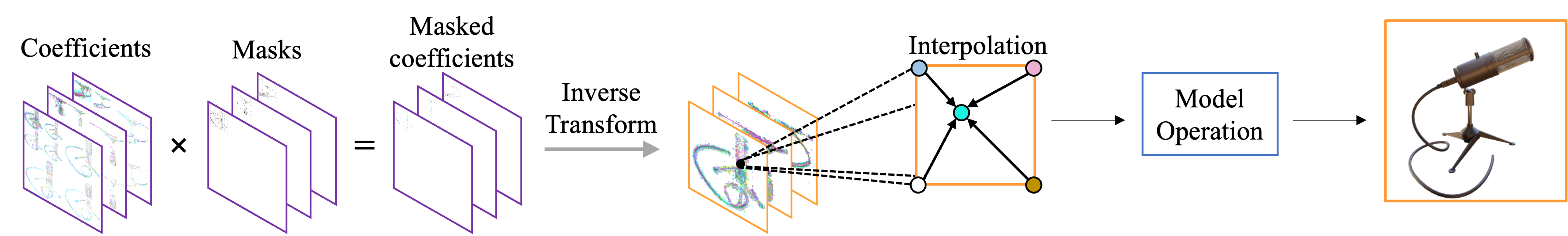
Figure 2: The overall architecture of our model. Images with purple borders illustrate wavelet coefficients, while those with orange borders visualize spatial coefficients. The wavelet coefficients in each 2D grid are multiplied with a binarized mask to form a masked wavelet coefficient grid. Masked wavelet coefficients are then inverse-transformed to spatial features. We sample feature vectors for input coordinates using bilinear interpolation on the grids. Then, opacity and color for each input coordinate are estimated using the sampled feature vectors following the defined model.

3 Methods

3.1 Neural radiance fields

We consider a neural radiance field leveraging grid representations. It takes an input coordinate $x\in\mathbb{R}^{3}$ and viewing direction, $d\in\mathbb{R}^{2}$, generating a four-dimensional vector consisting of a density and three-channel RGB colors, defined as follows.

$$\sigma(x)=f_{\sigma}(x;\gamma_{\sigma},\mathcal{M}_{\sigma}),$$ (1)

$$c(x,d)=f_{c}(x,d;\theta,\gamma_{c},\mathcal{M}_{c}),$$ (2)

where $\theta$ is the parameter of an MLP, $\gamma=\{\gamma_{\sigma},\gamma_{c}\}$ is a set of grid parameters, and $\mathcal{M}=\{\mathcal{M}_{\sigma},\mathcal{M}_{c}\}$ is a set of masks for grid parameters, which will be described shortly (Sec. 3.3). The following volumetric rendering equation is used to synthesize novel views:

$$C(r)=\int_{t_{n}}^{t_{f}}T(t)\sigma(r(t))c(r(t),d)dt,$$ (3)

$$T(t)=\text{exp}(-\int_{t_{n}}^{t}\sigma(r(s))ds),$$ (4)

where $r(t)$ is a ray from a camera viewpoint, and $C(r)$ is the expected color of the ray $r(t)$. Two integral bounds (near and far) are denoted as $t_{n}$ and $t_{f}$, respectively. Please refer to NeRF [23] for more details.

3.2 Wavelet transform on decomposed tensors

Frequency-based algorithms, such as discrete cosine transform (DCT) or discrete wavelet transform (DWT), have been developed and improved over the decades. For high compression performance, standard codecs have used them to make sparse representations. However, in the case of 3D grid representation, their computational complexity increases cubically with grid resolution, making high-resolution 3D scene and object representations impractical. In order to use frequency-based algorithms for compact representation, we need lower-dimensional data, such as 2D planes or 1D lines.

Recent studies have explored various decomposition methods to reduce the spatial complexity of 3D grid-based representations. Among them, plane-based representations have achieved remarkable success in reducing the number of parameters while maintaining the rendering performance [4, 3, 17]. They propose decomposing a 3D tensor into a set of 2D planes or 1D vectors.

To combine the best of both worlds, we propose using the wavelet transform on 2D plane-based neural fields [4]. We use the wavelet transform because of its compactness, especially for non-repeating, non-smooth signals.

For efficient 3D object and scene representation, recent studies proposed using a lower-dimensional grid (2D planes or 1D lines) [3, 4]. For example, EG3D [3] utilizes three 2D planes (tri-plane) and TensoRF [4] employs three sets, each consisting of a plane and a vector. We describe our method based on TensoRF. In detail, we use a set of 2D matrices and 1D vectors for grid representation, $\gamma_{\sigma}=\{\mathcal{W}_{\sigma,r}^{x},\mathcal{W}_{\sigma,r}^{y},\mathcal{W}_{\sigma,r}^{z},v_{\sigma,r}^{x},v_{\sigma,r}^{y},v_{\sigma,r}^{z}\}_{r=1}^{N_{\sigma,r}}$ ($\sigma$ denotes density, and we will omit the subscript $\sigma$ for brevity from now on) as proposed in TensoRF [4]. $N_{r}$ is the number of ranks in matrix-vector decomposition and $\mathcal{W}_{r}^{x}\in\mathbb{R}^{H\times W}$, $\mathcal{W}_{r}^{y}\in\mathbb{R}^{W\times D}$, $\mathcal{W}_{r}^{z}\in\mathbb{R}^{H\times D}$ are matrices, $v_{r}^{x}\in\mathbb{R}^{D}$, $v_{r}^{y}\in\mathbb{R}^{H}$, $v_{r}^{z}\in\mathbb{R}^{W}$, are vectors in $x,y,z$ directions, respectively. $H,W,D$ are the resolution of the grid. More formally, a 3D grid representation $G$ can be defined as follows.

$$G=\sum_{r=1}^{N_{r}}\sum_{d\in\{x,y,z\}}v_{r}^{d}\otimes\texttt{idwt}(\mathcal{W}_{r}^{d}),$$ (5)

where $\otimes$ denotes the outer product and $\texttt{idwt}(\cdot)$ is a two-dimensional inverse discrete wavelet transform (IDWT).

With a slight abuse of notation, a single level IDWT of a matrix $\mathcal{W}\in\mathcal{R}^{m\times n}$ can be written as follows.

$$\texttt{idwt}(\mathcal{W})=\Phi\star(\uparrow 2)(\mathcal{W}_{LL})+\Psi_{HL}\star(\uparrow 2)(\mathcal{W}_{HL})$$ (6)

$$+\Psi_{LH}\star(\uparrow 2)(\mathcal{W}_{LH})+\Psi_{HH}\star(\uparrow 2)(\mathcal{W}_{HH}),$$

where $\mathcal{W}_{LL},\mathcal{W}_{HL},\mathcal{W}_{LH},\mathcal{W}_{HH}\in\mathbb{R}^{m/2\times n/2}$ denote approximation, horizontal, vertical, and diagonal coefficients, respectively. $\star$ denotes 2D cross correlation and $(\uparrow 2):\mathbb{R}^{m/2\times n/2}\rightarrow\mathbb{R}^{m\times n}$ denotes (nearest neighbor) upscaling. $\Psi$ and $\Phi$ are wavelet function and scaling function, respectively. We use the biorthogonal 4.4 wavelet function and its corresponding scaling function [6]. Even though we follow the grid representation of TensoRF, our method is not limited to the existing 2D plane-based representations but can be applied to any other approaches that adopt 2D planes to represent higher-dimensional structures.

As shown in Eq. 5, we only apply IDWT over matrices $\mathcal{W}$ since we observed that IDWT to vectors resulted in significant quality degradation. As this transformation is differentiable, the model can be trained end-to-end. We can also obtain the 3D grid representation for appearance through the same process and provide all formulations in the supplementary material.

Our method incurs insignificant costs during inference. Once training is finished, only one IDWT per grid is needed to transform wavelet grids into spatial grids. Thus, the remaining computational costs and time are exactly the same as the original spatial grid-based neural fields.

3.2.1 Multi-level wavelet transform

To further improve parameter sparsity and reconstruction quality, we propose using a multi-level wavelet transform. We experimentally found that higher-level wavelet transformations result in higher sparsity in grids (Sec. 4.3.1). However, naively using a multi-level wavelet transform on grid parameters degrades the representation quality (Tab. 1). We hypothesize that this is because the range of wavelet coefficients and the range of their gradients vary depending on the level of decomposition. In more detail, high-pass coefficients typically have a larger gradient scale with a smaller weight range. Different weight scales and gradients for different frequencies seem to hinder the optimization process. As such, we propose multiplying wavelet coefficients by the scales proportional to the inverse of frequency. With our proposed scaling factors $s$, Eq. 5 can be rewritten as follows.

$$G=\sum_{r=1}^{N_{r}}\sum_{d\in\{x,y,z\}}v_{r}^{d}\otimes\texttt{idwt}(\mathcal{W}_{r}^{d}\odot s_{r}^{d}),$$ (7)

where $\odot$ denotes the Hadamard product. For example, a two-level DWT, as shown in Fig. 3, generates a total of seven groups of coefficients (LL2, HL2, LH2, HH2, HL1, LH1, HH1). The scaling factors $s$ for HL2, LH2, and HH2 will be set to 1/2, and for HL1, LH1, and HH1 to 1/3. This scaling method enhances the quality of the reconstruction; more experiments are described in Sec. 4.3.2.

3.3 Learning to mask

Even though Wavelet coefficients can be sparse, we need additional methods to attain higher sparsity. Thus, we propose using element-wise masks to increase the portion of zero elements in grids. By jointly optimizing binary masks and grid parameters, we aim to zero out the majority of coefficients without significantly degrading the rendering quality. As we defined earlier, we have a set of trainable element-wise masks, $\mathcal{M}=\{\mathcal{M}_{r}^{x},\mathcal{M}_{r}^{y},\mathcal{M}_{r}^{z},m_{r}^{x},m_{r}^{y},m_{r}^{z}\}_{r=1}^{N_{r}}$ (note that we omitted the subscript $\sigma$ for brevity). During training, the grid parameters and corresponding binarized masks are multiplied element by element. Since calculating gradients directly from binarized masks is not feasible, we used the straight-through-estimator technique [1] to train and use masks. Formally, the masked matrix parameters $\widehat{\mathcal{W}}_{r}$ for $\mathcal{W}_{r}$ can be expressed as follows,

$$\widehat{\mathcal{W}}_{r}=\texttt{sg}((\mathcal{H}(\mathcal{M}_{r})-\sigma(\mathcal{M}_{r}))\odot\mathcal{W}_{r})+\sigma(\mathcal{M}_{r})\odot\mathcal{W}_{r},$$ (8)

where $\texttt{sg}(\cdot)$ is the stop-gradient operator. $\sigma(\cdot)$ and $\mathcal{H}(\cdot)$ denote the element-wise sigmoid and Heaviside step function, respectively. We can also compute the masked vector parameters $\widehat{v}_{r}$ similarly. By replacing grid parameters ($\mathcal{W}_{r}$, $v_{r}$) from Eq. 7 with masked grid parameters ($\widehat{\mathcal{W}}_{r}$, $\widehat{v}_{r}$), we can represent a masked 3D grid representation as follows:

$$G=\sum_{r=1}^{N_{r}}\sum_{d\in\{x,y,z\}}\widehat{v}_{r}^{d}\otimes\texttt{idwt}(\widehat{\mathcal{W}}_{r}^{d}\odot s_{r}^{d})$$ (9)

To make binarized mask values sparse, we use the sum of all mask values as the additional loss term $\mathcal{L}_{m}$. The overall loss function is a sum of rendering loss $\mathcal{L}_{r}$ and the mask regularization term $\mathcal{L}_{m}$.

$$\mathcal{L}=\mathcal{L}_{r}+\lambda_{m}\mathcal{L}_{m}.$$ (10)

We use $\lambda_{m}$ to control the sparsity of the parameters of the grid representation.

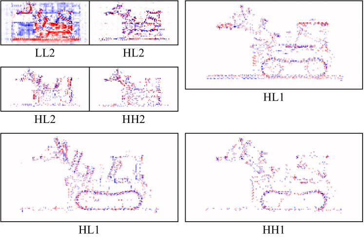
Figure 3: Multi-level discrete wavelet coefficients (2-level). LL, HL, LH, and HH denote approximation, horizontal, vertical, and diagonal coefficients, respectively. The numbers on the right denote the level of decomposition.

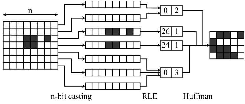
Figure 4: Proposed bitmap compression pipeline. RLE and Huffman denote run-length encoding and Huffman encoding, respectively.

3.4 Compression pipeline

With our proposed masking method and multi-level DWT, the ratio of zeros in grids can go up to more than 95%. However, sparse representations themselves do not reduce the total size. In this section, we describe our proposed compression pipeline for sparse grid parameters. Instead of storing grids as they are, we separately store non-zero coefficients and bitmaps (or masks) that indicate which coefficients are non-zero. Despite using 1-bit bitmaps, the overall bitmap size is large due to the large number of parameters. To reduce the bitmap sizes, we propose a compression pipeline with the following three stages: n-bit casting, run-length encoding (RLE), and the Huffman encoding [19]. The compression pipeline is illustrated in Fig. 4.

Before applying the compression pipeline, we split wavelet coefficient masks by level of decomposition. For the 2-level wavelet transform, for instance, we group HL1, LH1, and HH1, then HL2, LH2, and HH2, and finally LL2 (Fig. 3). This is based on our experimental results that wavelet coefficients with the same levels of sparsity have similar levels of sparsity (Fig. 6). We found that grouping coefficients with similar sparsity results in better compression performance. In addition, we found that directly applying RLE to 1-bit streams causes inefficient bit allocation due to the numerous repeating zeros. Therefore, we first cast the binary mask values to n-bit unsigned integers, and perform RLE afterward. In our experiments, we set n to 8. Finally, we apply the Huffman encoding algorithm to the RLE-encoded streams to map values with a high probability to shorter bits.

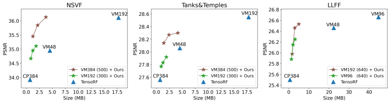
Figure 5: Rate distortion curves on the NSVF synthetic, TanksAndTemples, and LLFF dataset. We used 8-bit precision for every method.

4 Experiments

4.1 Experimental settings

We compared our proposed method with other baselines in four datasets; NeRF synthetic dataset [23], Neural Sparse Voxel Fields (NSVF) [22] dataset, TanksAndTemples dataset [20], and LLFF dataset [10].

We used TensoRF VM-192 as the baseline model and applied the proposed method. To control the size of our method, we adjusted the mask regularization weight $\lambda_{m}$, the number of grid channels (from VM-192 to VM-384), and the resolution of grids. Unless otherwise specified, we used 8-bit quantization for every method. We compared our method with quantized NeRF, TensoRF models (CP and VM), cNeRF [2] and CCNeRF [43]. We also tried to compare our approach with VQAD [39], which efficiently compresses 3D scene representations using codebooks and vector quantization. However, VQAD requires depth maps to prune out vacant areas in advance. Otherwise, the required memory exceeds the memory capacity of the Tesla A100 equipped with 40 GB of memory. Since the datasets we used do not provide depth maps, we did not compare VQAD with ours.

We followed the experimental settings of TensoRF [4]. We trained models for 30,000 iterations, each of which is a minibatch of 4,096 rays. We used the Adam optimizer and an exponential learning rate decay scheduler. Following TensoRF, the initial learning rates of grid-related parameters and MLP-related parameters were set to 0.02 and 0.001, respectively. Final learning rates were set at 1/10 of the initial learning rate. We updated the alpha masks at the 2000th, 4000th, 6000th, 11000th, 16000th, 21000th, and 26000th iterations. We set $\lambda_{m}$ in Eq. 10 to 1e-10 for high parameter sparsity and 5e-11 and 2.5e-11 for relatively lower sparsity. We set the initial values of masks $\mathcal{M}$ to one, and set their initial learning rate to the same learning rate as grid parameters $\phi$. As a reconstruction quality measurement, we used PSNR.

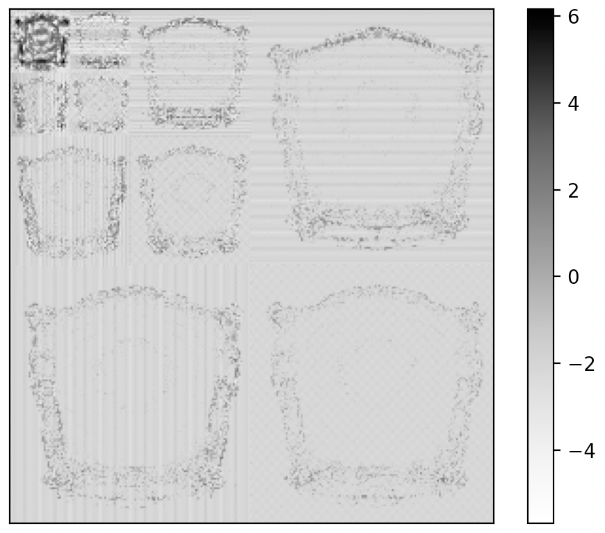
(a) Raw mask

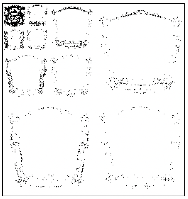
(b) Binarized mask

Figure 6: Qualitative analysis on mask $\mathcal{M}$ (Chair in the NeRF synthetic dataset).

4.2 Results

Figs. 1 and 5 show the quantitative performances of our method and the baselines on various datasets. Each graph displays the average PSNR and size of methods. More detailed numbers are available in the supplementary materials.

As the rate-distortion curves show, our method achieves higher efficiency than the baseline models and other methods. Even with the base network (VM-192), our method consistently outperforms other baselines on all novel view synthesis datasets, under a small memory budget of 2 MB. We adjusted both $\lambda_{m}$ and the network size to increase the output size. By adjusting $lambda_{m}$, we can control both size and quality while having no effect on computational costs, time, or memory requirements. Increasing network size (doubling the number of channels and increasing the resolution) can push the boundary even further. It is also worth mentioning that applying our method to a larger backbone model (VM-384) outperforms models with a smaller backbone model (VM-192), even with the same value of $\lambda_{m}$ or a similar model size. However, as the network grows in size, the computational costs and time required for training and testing increase. Therefore, it is still reasonable to use a small backbone model when using our proposed method.

Fig. 7 shows the qualitative results with and without our proposed masking method. Trainable masks removed more than 97% of the grid parameters; nevertheless, the rendered results are still accurate, and the qualitative difference is almost imperceptible. This demonstrates that our proposed method efficiently eliminates unnecessary wavelet coefficients by leveraging trainable masks.

Fig. 6 illustrates both raw and binarized masks after training. First of all, sparsity varies depending on the level of the wavelet transform. As shown in Fig. 6(b), coefficients with lower frequencies have lower sparsity, whereas coefficients with higher frequencies have higher sparsity. What is interesting is that the raw mask values seem to reflect the characteristics of corresponding wavelet coefficients. Vertical, horizontal, and diagonal patterns can be found in the raw mask values for the vertical, horizontal, and diagonal coefficients, respectively.

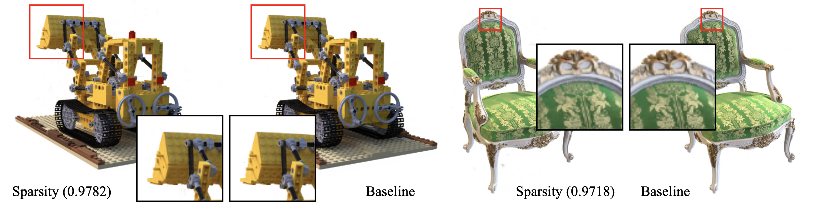
Figure 7: A qualitative analysis of grid sparsity. The sparsity refers to the ratio of zero elements in grids. With the help of trainable masks, removing more than 97% of grid parameters only results in an imperceptible difference.

4.3 Ablation studies

In this section, we analyze each component of our proposed method. Every experiment was conducted on the whole NeRF synthetic dataset, and we used the average PSNR as a measurement for representation quality. We used 4-level wavelet transform and set $\lambda_{m}$ to 1e-10, unless otherwise specified.

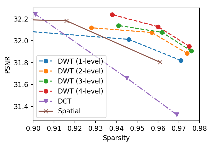
Figure 8: The rate distortion curves of different signal representation schemes (spatial, DWT, and DCT). Sparsity on the x axis refers to the ratio of zeros in grid parameters. The grid sparsity was controlled by $\lambda_{m}$. The numbers inside the parenthesis indicate the levels of the wavelet transform.

4.3.1 Discrete wavelet transform

In this section, we evaluate the compactness of wavelet coefficients and the performance improvements brought by the multi-level wavelet transform. Fig. 8 shows the rate-distortion curves of four different levels of wavelet transform and non-wavelet coefficients. As shown in the figure, wavelet-based grid representation outperforms the grid in the spatial domain, especially when the sparsity is high. Furthermore, rate-distortion curves demonstrate that higher level of wavelet transform improves visual quality and sparsity.

4.3.2 Level-wise wavelet coefficient scaling

As mentioned in Sec. 3.2.1, we proposed multiplying wavelet coefficients by the scales proportional to the inverse of frequency. Thus, we compared two versions of wavelet transform; one with our proposed weight scaling (Sec. 3.2.1) and the other without it. As Tab. 1 shows, scaling wavelet coefficients improves reconstruction performance.

Methods	PSNR
DWT	31.949
DWT w/o level-wise scaling	31.145
DCT	31.325

Table 1: Ablation study on level-wise scaling. Without our proposed scaling method, the performance of DWT is worse than DCT.

Wavelet Function	PSNR
Haar	31.889
Coiflets 1	31.846
Daubechies 4	31.734
biorthogonal 4.4 (default)	31.949
reverse biorthogonal 4.4	31.727

Table 2: Reconstruction performances of different wavelet functions.

4.3.3 Wavelet functions

In this section, we analyze how different wavelet functions affect reconstruction quality. For comparison, we selected several wavelet functions: Haar, Coiflet 1, Daubechies 4, and reverse biorthogonal 4.4. As shown in Tab. 2, the type of wavelet function has little effect on reconstruction quality. Even Haar, the simplest wavelet function, performs fairly well. Still, the biorthogonal 4.4 that we used shows the best performance among selected wavelet functions.

4.3.4 Discrete cosine transform

In this section, we compare the performance of DWT with that of DCT, which represents a signal with respect to the sum of cosine functions with different frequencies. DCT, similar to DWT, has an energy compaction property. That is, a small number of non-zero DCT coefficients are sufficient to represent a given signal. Because of its energy compactness, DCT or its variants are another widely used signal transformation for image, audio, and audio compression. However, as shown in Fig. 8 and Tab. 1, DWT shows superior compression and representation performance to DCT. We believe this is due to the non-repeating, non-smooth information in grids, for which DWT is more appropriate.

5 Conclusion

We propose a compact representation for grid-based neural fields, enabled by a novel masking strategy and multi-level wavelet transform. We demonstrate that these two components made it possible to remove more than 95% of grid parameters without a significant loss of visual quality. With our proposed compression pipeline and the sparse wavelet coefficients, we achieved state-of-the-art performance under a memory budget of 2 MB. We believe we can reduce the size further with more sophisticated compression pipelines.

Our proposed method is naturally constrained by the limitations of grid-based neural fields that are developed for bounded scenes or objects. We believe that expanding this grid-based representation to encompass unbounded or large scenes would be an intriguing direction, given that we can now compactly represent 3D objects with our proposed representation scheme.

Masked Wavelet Representation for Compact Neural Radiance Fields:
Supplementary Materials

Appendix A Qualitative Comparison

In this section, we visually demonstrate the qualities of neural fields with similar sizes. Fig. 9 shows the qualitative results of similar-sized representations: TensoRF-CP-384, NeRF, and Ours ($\lambda_{m}$=1e-10). The bit precision of each model was set to 8 bits. Even though they have similar overall sizes (less than 1 MB), ours shows the best qualitative results.

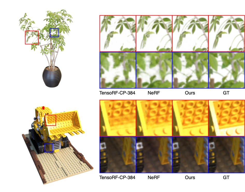
Figure 9: Qualitative analysis of similar-sized representations. Every method was quantized to 8 bits and less than 1 MB.

Appendix B Computational Costs

We also present the computational costs, particularly in terms of time, because we introduced learnable masks and DWT for efficient scene representation. First of all, as we explained in the main paper, we can ignore the computational costs at inference time. However, those two components incur non-negligible training time during training time. Tab. 3 shows the approximate training time to train a network (VM-192). It was evaluated using a 40 GB memory-equipped Tesla A100. Introducing masks increases the training time, but by a relatively insignificant amount of time. On the other hand, DWT increases training time more significantly. We believe that the increased training time is due to two factors: additional computational costs caused by DWT and not fully optimized DWT codes. As a result, we believe future DWT code optimization can help close this training time gap, especially given that current codes lower the GPU utilization rate from 80% (baseline) to 50% (4-level DWT with mask). Nevertheless, the time required by our proposed method is still far less than that of neural fields that exclusively use MLP, such NeRF.

	No Mask	Mask
Spatial	$\approx$ 8 min	$\approx$ 9 min
1-level DWT	$\approx$ 13 min	$\approx$ 14 min
2-level DWT	$\approx$ 15 min	$\approx$ 17 min
3-level DWT	$\approx$ 18 min	$\approx$ 20 min
4-level DWT	$\approx$ 23 min	$\approx$ 24 min

Table 3: Approximate training time

Appendix C Comparison on Masking Method

Methods	Sparsity	PSNR
Abs. Thres. ($\tau$=0.5)	0.8554	32.33
Abs. Thres. ($\tau$=1.0)	0.9385	28.95
Abs. Thres. ($\tau$=1.6)	0.9747	21.40
Ours ($\lambda_{m}$=2.5e-11)	0.9376	32.24
Ours ($\lambda_{m}$=1.0e-10)	0.9769	31.95

Table 4: Pruning on NeRF Synthetic dataset. The threshold of the absolute value-based method (Abs. Thres.), is denoted as $\tau$.

We also compared our masking method with a threshold-based pruning approach that removes grid coefficients whose absolute values are below a threshold $\tau$. As Tab. 4 shows, ours is more parameter-efficient than the threshold-based pruning method. It further supports the effectiveness of our proposed masking method in improving efficiency.

Appendix D Ablation Studies on Mask Compression

Lv. wise.	8-bit.	RLE	Huffman	Avg	Chair	Drums	Ficus	Hotdog	Lego	Materials	Mic	Ship
				2.07	1.96	2.01	2.07	2.24	1.99	2.37	1.91	2.02
		$\surd$		1.19 (1.75)	1.39 (1.41)	1.58 (1.27)	1.47 (1.41)	0.70 (3.21)	1.08 (1.84)	1.46 (1.62)	0.73 (2.62)	1.08 (1.87)
		$\surd$	$\surd$	0.45 (4.62)	0.52 (3.75)	0.59 (3.38)	0.55 (3.74)	0.26 (8.49)	0.41 (4.82)	0.55 (4.32)	0.28 (6.78)	0.41 (4.89)
	$\surd$	$\surd$	$\surd$	0.33 (6.24)	0.40 (4.88)	0.42 (4.41)	0.42 (4.93)	0.18 (12.71)	0.31 (6.48)	0.39 (6.05)	0.20 (9.50)	0.30 (6.68)
$\surd$	$\surd$	$\surd$	$\surd$	0.28 (7.39)	0.36 (5.47)	0.35 (5.60)	0.35 (5.91)	0.16 (13.92)	0.26 (7.61)	0.34 (6.97)	0.16 (12.13)	0.26 (7.88)

Table 5: The mask size and compression ratio at each stage of the compression pipeline evaluated on the NeRF synthetic dataset. Each number is in megabytes, and the number inside parenthesis indicates the compression ratio. RLE and Huffman indicate run-length and Huffman encoding, respectively. Level-wise encoding and 8-bit casting are denoted as “Lv. wise.” and “8-bit.”. The first row shows the original binarized mask size.

Methods	size(MB)	Avg	Chair	Drums	Ficus	Hotdog	Lego	Materials	Mic	Ship
Baseline	14.41	28.52	31.83	22.81	23.06	35.50	29.67	27.31	30.87	27.10
Ours ($\lambda_{m}$=1e-10)	0.71	27.91	30.69	23.18	23.22	33.18	38.85	27.09	30.29	26.79
Ours ($\lambda_{m}$=5e-11)	0.98	28.35	30.89	23.39	23.30	34.65	29.19	27.36	30.696	27.03
Ours ($\lambda_{m}$=2.5e-11)	1.38	28.39	31.07	23.18	23.27	34.78	29.18	27.44	31.05	27.14

Table 6: The performance of our proposed method with the tri-planar architecture on the NeRF synthetic dataset. Reconstruction quality was measured in PSNR. By setting $\lambda_{m}$ to 5e-11, our proposed method compresses the baseline model 14.70 times without significant PSNR loss.

	Plane	Lv. 1	Lv. 2	Lv. 3	Lv. 4 (precinct)	Lv. 4 (upper-left)
Density	YX	0.99	0.97	0.91	0.76	0.33
	ZX	0.99	0.96	0.91	0.82	0.36
	ZY	0.99	0.97	0.93	0.84	0.43
Appearance	YX	0.97	0.94	0.90	0.80	0.61
	ZX	0.98	0.96	0.93	0.87	0.63
	ZY	0.99	0.98	0.95	0.91	0.73

Table 7: Sparsity table of 4-level DWT with learnable mask ($\lambda_{m}$=1e-10) on Chair (from the NeRF dataset).

	no scan	zigzag	morton	spiral
Size (MB)	0.83	0.83	0.85	0.83

Table 8: Average size by scanning order on the NeRF synthetic dataset.

In this section, we analyze our proposed compression pipeline in more detail by demonstrating the compression ratio at each stage and outlining the rationale for our design decisions. Tab. 5 shows the compression ratios in the NeRF dataset. By incrementing each step, we demonstrate how each step contributes to the compression ratio. Keep in mind that we do not compress non-zero coefficients; we only compress information regarding which coefficients are non-zero (mask). We keep the non-zero coefficients that are not compressed as well as the compressed mask that shows where the non-zero components are located.

Run-length encoding (RLE) The RLE is effective for compressing data with repeating numbers. Instead of encoding raw repeating numbers, RLE encodes repeating numbers as a pair of the number and its count. This is why we adopt RLE in our mask compression pipeline. Our proposed method zeros out most grid coefficients. More specifically, by adopting our proposed method, the sparsity of grids can go up to 90% or even 99%. As shown in the second row of Tab. 5, adopting RLE can reduce the mask size by a factor of 1.75, on average.

Huffman encoding As shown in the third row of Tab. 5, we can raise the compression ratio to 4.62 by including Huffman encoding in our compression pipeline. We also compared adaptive arithmetic coding  [29] with Huffman encoding but did not observed meaningful improvements. As a result, we chose to use the less expensive Huffman encoding in our compression pipeline. We believe, however, that further improvements could be made by incorporating advanced compression techniques into the proposed method.

8-bit casting Packing the binarized mask values by 8 bits before applying RLE can further increase the compression ratio to 6.24 (Tab. 5). This is because the casting makes the length of the RLE code much shorter. For example, consider a thousand 0s. Without casting, we can represent a thousand 0s with three (0, 255) and one (0, 235). On the other hand, with the help of casting, we only need a pair of two numbers (0, 125). We use this method assuming most elements are zeros, and as shown in the table, it can really improve compression ratio.

Level-wise encoding We discovered that sparsity highly depends on the level of DWT, as shown in Tab. 7. More specifically, high-pass coefficients have higher sparsity. Based on the findings, we separate the mask at each level and compress separately. For the last level of DWT, we treat the upper left part (LL) and the remaining three parts (LH, HL, HH, also known as precincts) separately, as the former has much fewer zeros compared to the latter. As shown in Tab. 5, adding the level-wise encoding into the pipeline improves the compression ratio even further, resulting in an average size of 0.28 mb, which is 7.39 times smaller than the size of the original mask.

Scanning order Since scanning order before compression can affect the output size, we also tried different scanning orders and measure the output sizes. Tab. 8 shows the results on the NeRF synthetic dataset. As shown, scanning order did not affect the performance noticeably.

Appendix E Application to Other 2D Grid-based Neural Fields

Even though we only showed results using a TensoRF [4] model (VM-192), our proposed method is not confined to TensoRF. Only TensoRF was used in the main paper because it is currently the most effective method for plane-based neural fields.

To demonstrate that our method can be used with any grid-based neural representation, we apply it to additional plane-based neural fields in this section. We exclusively employed 2D grids, not 1D grids, as plane-based neural fields. This was only intended to demonstrate that our suggested method can be used with other 2D grid-based methods in addition to TensoRF. TriPlane from EG2D [3] served as the model for this design, which uses only 2D planes. The difference is that, like TensoRF, we separate the grids for density and appearance. For implementation, we removed 1D grids from the baseline model we used in the main paper.

As shown in Tab. 6, our proposed method can be successfully applied to other 2D grid-based representations and remove most of the coefficients without causing considerable quality degradation. When $\lambda_{m}$ was set to 5e-11, our proposed method reduced the size to less than 7% of its original size with negligible quality drops (0.17 drops measured in PSNR).

Appendix F Color Estimation in Detail

Following TensoRF [4], we use separate grids for density and appearance (color) estimation. In this section, we describe appearance grids in detail. Similar to density grids, we use three 2D matrices and three vectors, $\phi_{c}=\{\mathcal{W}_{c,r}^{x},\mathcal{W}_{c,r}^{y},\mathcal{W}_{c,r}^{z},v_{c,r}^{x},v_{c,r}^{y},v_{c,r}^{z}\}_{r=1}^{N_{c,r}}$ ($c$ denotes color, and we will omit the subscript $c$ for brevity from now on). $N_{r}$ is the number of ranks in matrix-vector decomposition and $\mathcal{W}_{r}^{x}\in\mathbb{R}^{H\times W}$, $\mathcal{W}_{r}^{y}\in\mathbb{R}^{W\times D}$, $\mathcal{W}_{r}^{z}\in\mathbb{R}^{H\times D}$ are matrices, $v_{r}^{x}\in\mathbb{R}^{D}$, $v_{r}^{y}\in\mathbb{R}^{H}$, $v_{r}^{z}\in\mathbb{R}^{W}$, are vectors in $x,y,z$ directions, respectively. $H,W,D$ denote the resolution of the grid. We employ DWT only over matrices, just as we did over density grids. Thus, $\mathcal{W}$ are wavelet coefficients, and $v$ are feature vectors in the spatial domain.

Density grids in TensoRF only generate a density value, while color grids generate a feature vector for each coordinate. These feature vectors are forwarded to MLP to estimate the colors. To extract a feature vector per coordinate, TensoRF uses additional vectors ($f^{x}$, $f^{y}$, $f^{z}$). More formally, a 3D grid representation $G_{c}$ can be defined as follows.

$$G_{c}=\sum_{r=1}^{N_{r}}\sum_{d\in\{x,y,z\}}v_{r}^{d}\otimes\texttt{idwt}(\mathcal{W}_{r}^{d})\otimes f_{r}^{d},$$ (11)

where $\otimes$ denotes the outer product and $\texttt{idwt}(\cdot)$ is a two-dimensional inverse discrete wavelet transform.

Appendix G Per-Scene Results

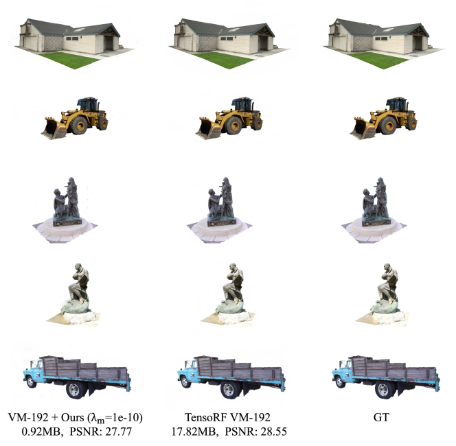
Figure 12: Qualitative results on the Tanks&Temples dataset.

In this section, we provide quantitative and qualitative results of each scene from NeRF synthetic, NSVF synthetic, TanksAndTemples, and LLFF dataset. Tabs. 9, 10, 11 and 12 show the quantitative results and Figs. 10, 11, 12 and 13 show the qualitative results on the four datasets.

Methods	size(MB)	Avg	Chair	Drums	Ficus	Hotdog	Lego	Materials	Mic	Ship
KiloNeRF ∘	$\leq$ 100	31.00	32.91	25.25	29.76	35.56	33.02	29.20	33.06	29.23
CCNeRF (CP) ∘	4.4	30.55	-	-	-	-	-	-	-	-
NeRF ∗	1.25	31.52	33.82	24.94	30.33	36.70	32.96	29.77	34.41	29.25
cNeRF ∙	0.70	30.49	32.28	24.85	30.58	34.95	31.98	29.17	32.21	28.24
PREF ∗	9.88	31.56	34.55	25.15	32.17	35.73	34.59	29.09	32.64	28.58
VM-192 ∗	17.93	32.91	35.64	25.98	33.57	37.26	36.04	29.87	34.33	30.64
VM-48 ∗	4.81	32.18	34.54	25.55	33.12	36.60	35.14	29.15	33.33	29.99
CP-384 ∗	0.72	31.18	33.49	25.11	29.86	35.97	33.26	29.56	33.56	28.59
VM-192 (300) + Ours ∗
$\lambda_{m}$=1e-10	0.83	31.95	34.14	25.53	32.87	36.08	34.93	29.42	33.48	29.15
$\lambda_{m}$=5e-11	1.16	32.13	34.52	25.66	33.03	36.20	35.16	29.58	33.68	29.19
$\lambda_{m}$=2.5e-11	1.69	32.24	34.68	25.56	33.17	36.37	35.50	29.56	33.74	29.34
VM-192 (500) + Ours ∗
$\lambda_{m}$=1e-10	1.02	32.14	34.64	25.55	33.04	35.85	35.15	29.54	33.91	29.41
$\lambda_{m}$=5e-11	1.55	32.37	34.90	25.69	33.25	36.13	35.50	29.63	34.21	29.65
$\lambda_{m}$=2.5e-11	2.36	32.46	35.16	25.77	33.34	36.26	35.74	29.65	34.19	29.57
VM-384 (300) + Ours ∗
$\lambda_{m}$=1e-10	0.99	32.08	34.32	25.50	33.28	36.22	34.83	29.91	33.36	29.20
$\lambda_{m}$=5e-11	1.50	32.23	34.59	25.55	33.41	36.35	35.13	29.95	33.47	29.42
$\lambda_{m}$=2.5e-11	2.42	32.38	34.84	25.58	33.59	36.66	35.46	29.94	33.56	29.43
VM-384 (500) + Ours ∗
$\lambda_{m}$=1e-10	1.23	32.36	34.85	25.75	33.49	36.05	35.11	29.86	34.16	29.65
$\lambda_{m}$=5e-11	2.03	32.66	35.35	25.75	33.71	36.55	35.69	29.91	34.46	29.89
$\lambda_{m}$=2.5e-11	3.36	32.77	35.49	25.78	33.78	36.79	35.85	29.94	34.56	30.01

Table 9: Performance on the NeRF synthetic dataset measured in PSNR. The performance of the 32-bit and 8-bit models described in the original paper are represented by the symbols ^∘ and ^∙, respectively. ^∗ denotes the performance of a quantized model with 8-bit precision. The number inside the parenthesis denotes the resolution of one axis of grids.

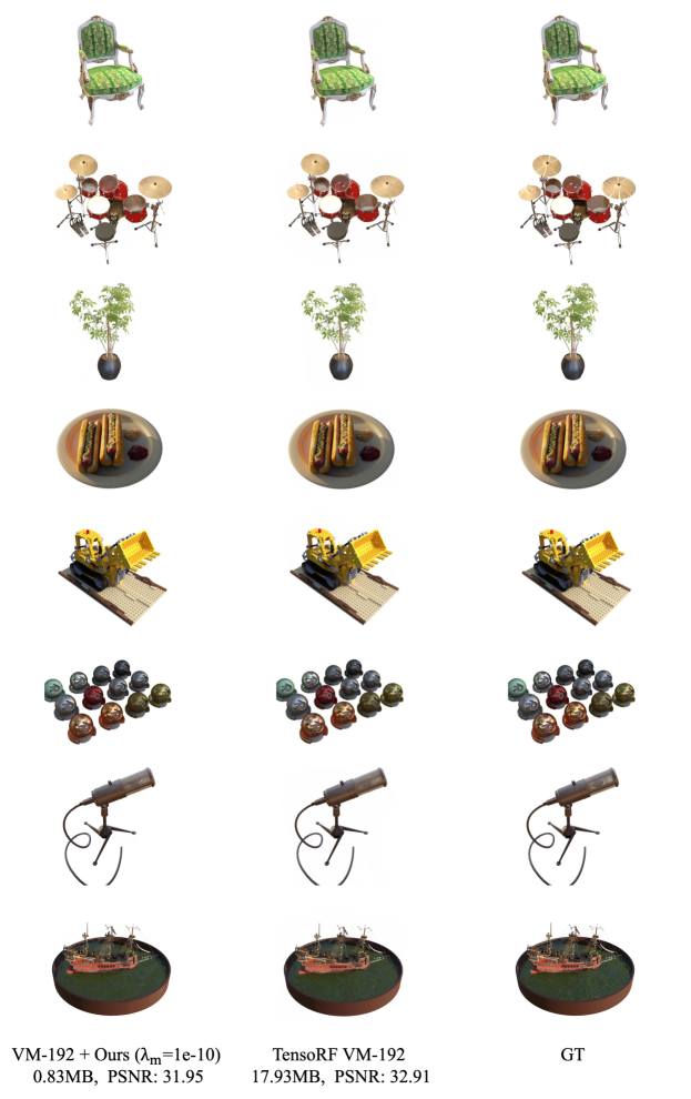
Figure 10: Qualitative results on the NeRF synthetic dataset.

Methods	size(MB)	Avg	Bike	Lifestyle	Palace	Robot	Spaceship	Steamtrain	Toad	Wineholder
KiloNeRF ∘	$\leq$ 100	33.37	35.49	33.15	34.42	32.93	36.48	33.36	31.41	29.72
VM-192 ∗	17.77	36.11	38.69	34.15	37.09	37.99	37.66	37.45	34.66	31.16
VM-48 ∗	4.53	34.95	37.55	33.34	35.84	36.60	36.38	36.68	32.97	30.26
CP-384 ∗	0.72	33.92	36.29	32.29	35.73	35.63	34.58	35.82	31.24	29.75
VM-192 (300) + Ours ∗
$\lambda_{m}$=1e-10	0.87	34.67	37.06	33.44	35.18	35.74	37.01	36.65	32.23	30.08
$\lambda_{m}$=5e-11	1.25	34.95	37.33	33.69	35.65	36.01	37.23	36.95	32.58	30.14
$\lambda_{m}$=2.5e-11	1.88	35.11	37.49	33.75	35.94	36.23	37.45	36.92	32.87	30.23
VM-192 (500) + Ours ∗
$\lambda_{m}$=1e-10	1.06	35.02	37.09	33.57	35.85	36.53	37.18	36.75	32.71	30.45
$\lambda_{m}$=5e-11	1.66	35.41	37.53	33.77	36.43	36.99	37.37	37.14	33.35	30.71
$\lambda_{m}$=2.5e-11	2.63	35.63	37.70	33.96	36.86	37.15	37.60	37.26	33.77	30.71
VM-384 (300) + Ours ∗
$\lambda_{m}$=1e-10	1.04	35.04	37.72	33.68	35.55	36.18	37.52	36.85	32.48	30.39
$\lambda_{m}$=5e-11	1.61	35.33	38.04	33.89	36.03	36.48	37.81	37.10	32.88	30.43
$\lambda_{m}$=2.5e-11	2.69	35.57	38.27	34.09	36.37	36.81	37.93	37.24	33.22	30.59
VM-384 (500) + Ours ∗
$\lambda_{m}$=1e-10	1.27	35.45	37.89	33.80	36.28	36.89	37.70	37.13	33.03	30.91
$\lambda_{m}$=5e-11	2.17	35.84	38.20	34.05	36.92	37.35	37.91	37.45	33.58	31.23
$\lambda_{m}$=2.5e-11	3.77	36.13	38.53	34.26	37.32	37.71	38.15	37.73	34.08	31.27

Table 10: Performance on the NSVF synthetic dataset measured in PSNR. The performance of the 32-bit models described in the original paper are represented by the symbols ^∘. ^∗ denotes the performance of a quantized model with 8-bit precision. The number inside the parenthesis denotes the resolution of one axis of grids.

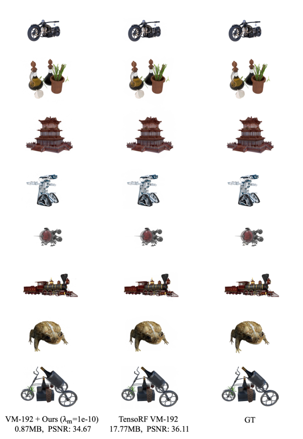
Figure 11: Qualitative results on the NSVF dataset.

Methods	size(MB)	average	Barn	Caterpillar	Family	Ignatius	Truck
KiloNeRF ∘	$\leq$ 100	28.41	27.81	25.61	33.65	27.92	27.04
CCNeRF (CP) ∘	4.4	27.01	-	-	-	-	-
VM-192 ∗	17.82	28.55	27.25	26.18	33.86	28.37	27.11
VM-48 ∗	4.52	28.06	26.77	25.46	33.06	28.24	26.77
CP-384 ∗	0.72	27.56	26.73	24.69	32.31	27.83	26.23
VM-192 (300) + Ours ∗
$\lambda_{m}$=1e-10	0.92	27.77	26.49	25.50	32.57	28.06	26.21
$\lambda_{m}$=5e-11	1.27	27.83	26.71	25.34	32.74	28.11	26.27
$\lambda_{m}$=2.5e-11	1.91	27.92	26.72	25.39	32.92	28.22	26.34
VM-192 (500) + Ours ∗
$\lambda_{m}$=1e-10	1.14	27.92	26.89	25.52	32.79	28.18	26.22
$\lambda_{m}$=5e-11	1.76	28.01	26.97	25.40	33.03	28.23	26.42
$\lambda_{m}$=2.5e-11	2.77	28.04	27.05	25.34	33.18	28.21	26.43
VM-384 (300) + Ours ∗
$\lambda_{m}$=1e-10	1.13	28.01	26.94	25.75	32.72	28.22	26.43
$\lambda_{m}$=5e-11	1.69	28.12	27.02	25.81	32.92	28.31	26.54
$\lambda_{m}$=2.5e-11	2.75	28.12	27.00	25.80	33.09	28.23	26.47
VM-384 (500) + Ours ∗
$\lambda_{m}$=1e-10	1.42	28.14	27.41	25.78	32.91	28.11	26.48
$\lambda_{m}$=5e-11	2.43	28.27	27.47	25.89	33.14	28.36	26.49
$\lambda_{m}$=2.5e-11	4.15	28.30	27.39	25.79	33.33	28.32	26.69

Table 11: Performance on the Tanks&Temples synthetic dataset measured in PSNR. The performance of the 32-bit models described in the original paper are represented by the symbols ^∘. ^∗ denotes the performance of a quantized model with 8-bit precision. The number inside the parenthesis denotes the resolution of one axis of grids.

Methods	size(MB)	Avg	Fern	Flower	Fortress	Horns	Leaves	Orchids	Room	T-Rex
cNeRF ∙	0.96	26.15	25.17	27.21	31.15	27.28	20.95	20.09	30.65	26.72
PREF ∗	9.34	24.50	23.32	26.37	29.71	25.24	20.21	19.02	28.45	23.67
VM-96 ∗	44.72	26.66	25.22	28.55	31.23	28.10	21.28	19.87	32.17	26.89
VM-48 ∗	22.40	26.46	25.27	28.19	31.06	27.59	21.33	20.03	31.70	26.54
CP-384 ∗	0.64	25.51	24.30	26.88	30.17	26.46	20.38	19.95	30.61	25.35
VM-96 (640) + Ours ∗
$\lambda_{m}$=1e-10	1.34	25.88	24.98	27.19	30.28	26.96	21.21	19.93	30.03	26.45
$\lambda_{m}$=5e-11	2.10	26.15	24.99	27.77	30.60	27.25	21.18	19.90	30.65	26.84
$\lambda_{m}$=2.5e-11	3.20	26.25	25.05	27.94	30.75	27.48	21.08	19.76	31.19	26.77
VM-96 (1000) + Ours ∗
$\lambda_{m}$=1e-10	1.75	25.82	24.97	27.44	30.29	26.92	21.11	20.09	29.27	26.47
$\lambda_{m}$=5e-11	3.01	26.17	25.05	27.70	30.71	27.29	21.09	20.01	30.91	26.62
$\lambda_{m}$=2.5e-11	4.76	26.30	25.08	27.76	30.89	27.49	21.14	19.99	31.23	26.85
VM-192 (640) + Ours ∗
$\lambda_{m}$=1e-10	1.73	25.98	25.18	27.47	29.66	27.47	21.11	19.71	30.47	26.79
$\lambda_{m}$=5e-11	3.01	26.46	25.12	28.16	30.81	27.88	21.07	19.77	31.61	27.28
$\lambda_{m}$=2.5e-11	5.04	26.53	25.05	28.15	30.99	28.09	20.97	19.75	31.85	27.40
VM-192 (1000) + Ours ∗
$\lambda_{m}$=1e-10	2.43	26.15	25.18	27.74	30.22	27.47	21.24	19.98	30.56	26.79
$\lambda_{m}$=5e-11	4.57	26.43	25.22	28.06	30.78	27.71	21.23	19.92	31.61	26.93
$\lambda_{m}$=2.5e-11	7.41	26.54	25.27	28.20	31.01	27.88	21.17	20.02	31.73	27.07

Table 12: Performance on the LLFF dataset measured in PSNR. The performance of the 8-bit models described in the original paper are represented by the symbol ^∙. ^∗ denotes the performance of a quantized model with 8-bit precision. The number inside the parenthesis denotes the resolution of one axis of grids.

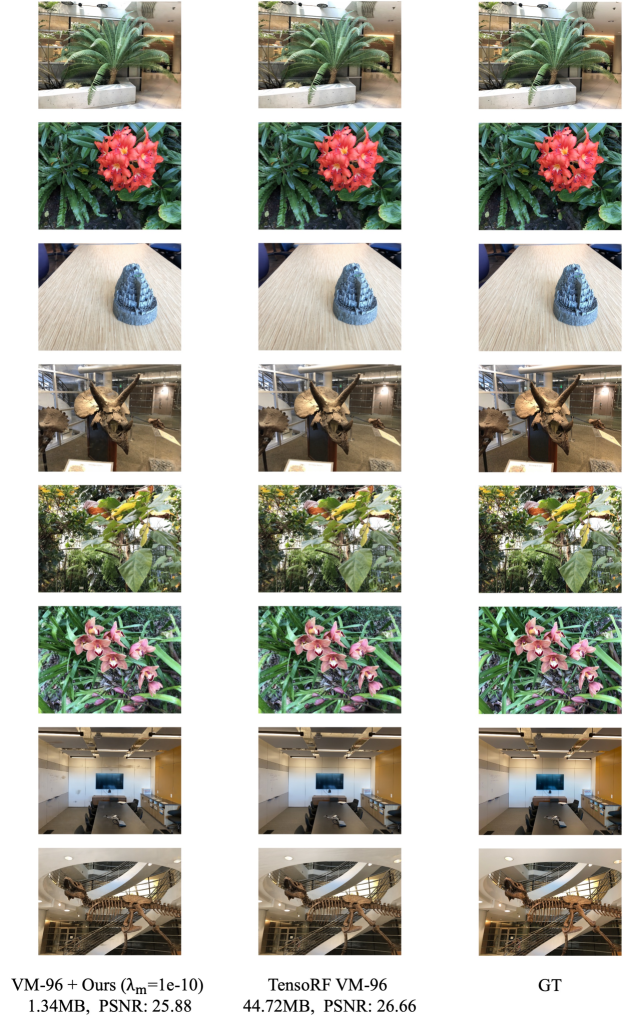
Figure 13: Qualitative results on the LLFF dataset.

References

- [1] Yoshua Bengio, Nicholas Léonard, and Aaron Courville. Estimating or propagating gradients through stochastic neurons for conditional computation. arXiv preprint arXiv:1308.3432, 2013.
- [2] Thomas Bird, Johannes Ballé, Saurabh Singh, and Philip A Chou. 3d scene compression through entropy penalized neural representation functions. In 2021 Picture Coding Symposium (PCS), pages 1–5. IEEE, 2021.
- [3] Eric R. Chan, Connor Z. Lin, Matthew A. Chan, Koki Nagano, Boxiao Pan, Shalini De Mello, Orazio Gallo, Leonidas J. Guibas, Jonathan Tremblay, Sameh Khamis, Tero Karras, and Gordon Wetzstein. Efficient geometry-aware 3d generative adversarial networks. In Proceedings of the IEEE/CVF Conference on Computer Vision and Pattern Recognition (CVPR), pages 16123–16133, June 2022.
- [4] Anpei Chen, Zexiang Xu, Andreas Geiger, Jingyi Yu, and Hao Su. Tensorf: Tensorial radiance fields. In European conference on computer vision. Springer, 2022.
- [5] Anpei Chen, Zexiang Xu, Fuqiang Zhao, Xiaoshuai Zhang, Fanbo Xiang, Jingyi Yu, and Hao Su. Mvsnerf: Fast generalizable radiance field reconstruction from multi-view stereo. In Proceedings of the IEEE/CVF International Conference on Computer Vision, pages 14124–14133, 2021.
- [6] Albert Cohen, Ingrid Daubechies, and J-C Feauveau. Biorthogonal bases of compactly supported wavelets. Communications on pure and applied mathematics, 45(5):485–560, 1992.
- [7] Matthieu Courbariaux, Yoshua Bengio, and Jean-Pierre David. Binaryconnect: Training deep neural networks with binary weights during propagations. In C. Cortes, N. Lawrence, D. Lee, M. Sugiyama, and R. Garnett, editors, Advances in Neural Information Processing Systems, volume 28. Curran Associates, Inc., 2015.
- [8] Chenxi Lola Deng and Enzo Tartaglione. Compressing explicit voxel grid representations: fast nerfs become also small. arXiv preprint arXiv:2210.12782, 2022.
- [9] Kangle Deng, Andrew Liu, Jun-Yan Zhu, and Deva Ramanan. Depth-supervised nerf: Fewer views and faster training for free. In Proceedings of the IEEE/CVF Conference on Computer Vision and Pattern Recognition, pages 12882–12891, 2022.
- [10] Ben Mildenhall et al. Local light field fusion: Practical view synthesis with prescriptive sampling guidelines. ACM Transactions on Graphics (TOG), 2019.
- [11] Jiemin Fang, Taoran Yi, Xinggang Wang, Lingxi Xie, Xiaopeng Zhang, Wenyu Liu, Matthias Nießner, and Qi Tian. Fast dynamic radiance fields with time-aware neural voxels. In SIGGRAPH Asia 2022 Conference Papers, SA ’22, New York, NY, USA, 2022. Association for Computing Machinery.
- [12] Chelsea Finn, Pieter Abbeel, and Sergey Levine. Model-agnostic meta-learning for fast adaptation of deep networks. In Doina Precup and Yee Whye Teh, editors, Proceedings of the 34th International Conference on Machine Learning, volume 70 of Proceedings of Machine Learning Research, pages 1126–1135. PMLR, 06–11 Aug 2017.
- [13] Sara Fridovich-Keil, Alex Yu, Matthew Tancik, Qinhong Chen, Benjamin Recht, and Angjoo Kanazawa. Plenoxels: Radiance fields without neural networks. In Proceedings of the IEEE/CVF Conference on Computer Vision and Pattern Recognition (CVPR), pages 5501–5510, June 2022.
- [14] Stephan J. Garbin, Marek Kowalski, Matthew Johnson, Jamie Shotton, and Julien Valentin. Fastnerf: High-fidelity neural rendering at 200fps. In Proceedings of the IEEE/CVF International Conference on Computer Vision (ICCV), pages 14346–14355, October 2021.
- [15] Peter Hedman, Pratul P. Srinivasan, Ben Mildenhall, Jonathan T. Barron, and Paul Debevec. Baking neural radiance fields for real-time view synthesis. pages 5875–5884, October 2021.
- [16] Tao Hu, Shu Liu, Yilun Chen, Tiancheng Shen, and Jiaya Jia. Efficientnerf efficient neural radiance fields. In Proceedings of the IEEE/CVF Conference on Computer Vision and Pattern Recognition (CVPR), pages 12902–12911, June 2022.
- [17] Binbin Huang, Xinhao Yan, Anpei Chen, Shenghua Gao, and Jingyi Yu. Pref: Phasorial embedding fields for compact neural representations. arXiv preprint arXiv:2205.13524, 2022.
- [18] Itay Hubara, Matthieu Courbariaux, Daniel Soudry, Ran El-Yaniv, and Yoshua Bengio. Binarized neural networks. In D. Lee, M. Sugiyama, U. Luxburg, I. Guyon, and R. Garnett, editors, Advances in Neural Information Processing Systems, volume 29. Curran Associates, Inc., 2016.
- [19] David A Huffman. A method for the construction of minimum-redundancy codes. Proceedings of the IRE, 40(9):1098–1101, 1952.
- [20] Arno Knapitsch, Jaesik Park, Qian-Yi Zhou, and Vladlen Koltun. Tanks and temples: Benchmarking large-scale scene reconstruction. ACM Trans. Graph., 36(4), jul 2017.
- [21] Yuhang Li, Ruihao Gong, Xu Tan, Yang Yang, Peng Hu, Qi Zhang, Fengwei Yu, Wei Wang, and Shi Gu. Brecq: Pushing the limit of post-training quantization by block reconstruction. arXiv preprint arXiv:2102.05426, 2021.
- [22] Lingjie Liu, Jiatao Gu, Kyaw Zaw Lin, Tat-Seng Chua, and Christian Theobalt. Neural sparse voxel fields. In H. Larochelle, M. Ranzato, R. Hadsell, M.F. Balcan, and H. Lin, editors, Advances in Neural Information Processing Systems, volume 33, pages 15651–15663. Curran Associates, Inc., 2020.
- [23] Ben Mildenhall, Pratul P Srinivasan, Matthew Tancik, Jonathan T Barron, Ravi Ramamoorthi, and Ren Ng. Nerf: Representing scenes as neural radiance fields for view synthesis. In European conference on computer vision, pages 405–421. Springer, 2020.
- [24] Thomas Müller, Alex Evans, Christoph Schied, and Alexander Keller. Instant neural graphics primitives with a multiresolution hash encoding. ACM Trans. Graph., 41(4), jul 2022.
- [25] Markus Nagel, Rana Ali Amjad, Mart Van Baalen, Christos Louizos, and Tijmen Blankevoort. Up or down? Adaptive rounding for post-training quantization. In Hal Daumé III and Aarti Singh, editors, Proceedings of the 37th International Conference on Machine Learning, volume 119 of Proceedings of Machine Learning Research, pages 7197–7206. PMLR, 13–18 Jul 2020.
- [26] Alex Nichol, Joshua Achiam, and John Schulman. On first-order meta-learning algorithms. arXiv preprint arXiv:1803.02999, 2018.
- [27] Julian Ost, Issam Laradji, Alejandro Newell, Yuval Bahat, and Felix Heide. Neural point light fields. pages 18419–18429, June 2022.
- [28] Songyou Peng, Chiyu Jiang, Yiyi Liao, Michael Niemeyer, Marc Pollefeys, and Andreas Geiger. Shape as points: A differentiable poisson solver. In M. Ranzato, A. Beygelzimer, Y. Dauphin, P.S. Liang, and J. Wortman Vaughan, editors, Advances in Neural Information Processing Systems, volume 34, pages 13032–13044. Curran Associates, Inc., 2021.
- [29] W. B. Pennebaker et al. An overview of the basic principles of the q-coder adaptive binary arithmetic coder. IBM Journal of Research and Development, 1988.
- [30] Aniruddh Raghu, Maithra Raghu, Samy Bengio, and Oriol Vinyals. Rapid learning or feature reuse? towards understanding the effectiveness of maml. arXiv preprint arXiv:1909.09157, 2019.
- [31] Mohammad Rastegari, Vicente Ordonez, Joseph Redmon, and Ali Farhadi. Xnor-net: Imagenet classification using binary convolutional neural networks. In Bastian Leibe, Jiri Matas, Nicu Sebe, and Max Welling, editors, Computer Vision – ECCV 2016, pages 525–542, Cham, 2016. Springer International Publishing.
- [32] Daniel Rebain, Wei Jiang, Soroosh Yazdani, Ke Li, Kwang Moo Yi, and Andrea Tagliasacchi. Derf: Decomposed radiance fields. In Proceedings of the IEEE/CVF Conference on Computer Vision and Pattern Recognition, pages 14153–14161, 2021.
- [33] Christian Reiser, Songyou Peng, Yiyi Liao, and Andreas Geiger. Kilonerf: Speeding up neural radiance fields with thousands of tiny mlps. In Proceedings of the IEEE/CVF International Conference on Computer Vision (ICCV), pages 14335–14345, October 2021.
- [34] Katja Schwarz, Axel Sauer, Michael Niemeyer, Yiyi Liao, and Andreas Geiger. VoxGRAF: Fast 3d-aware image synthesis with sparse voxel grids. In Alice H. Oh, Alekh Agarwal, Danielle Belgrave, and Kyunghyun Cho, editors, Advances in Neural Information Processing Systems, 2022.
- [35] Vincent Sitzmann, Eric Chan, Richard Tucker, Noah Snavely, and Gordon Wetzstein. Metasdf: Meta-learning signed distance functions. In H. Larochelle, M. Ranzato, R. Hadsell, M.F. Balcan, and H. Lin, editors, Advances in Neural Information Processing Systems, volume 33, pages 10136–10147. Curran Associates, Inc., 2020.
- [36] Athanassios Skodras, Charilaos Christopoulos, and Touradj Ebrahimi. The jpeg 2000 still image compression standard. IEEE Signal processing magazine, 18(5):36–58, 2001.
- [37] Gary J Sullivan, Jens-Rainer Ohm, Woo-Jin Han, and Thomas Wiegand. Overview of the high efficiency video coding (hevc) standard. IEEE Transactions on circuits and systems for video technology, 22(12):1649–1668, 2012.
- [38] Cheng Sun, Min Sun, and Hwann-Tzong Chen. Direct voxel grid optimization: Super-fast convergence for radiance fields reconstruction. In Proceedings of the IEEE/CVF Conference on Computer Vision and Pattern Recognition (CVPR), pages 5459–5469, June 2022.
- [39] Towaki Takikawa, Alex Evans, Jonathan Tremblay, Thomas Müller, Morgan McGuire, Alec Jacobson, and Sanja Fidler. Variable bitrate neural fields. In ACM SIGGRAPH 2022 Conference Proceedings, SIGGRAPH ’22, New York, NY, USA, 2022. Association for Computing Machinery.
- [40] Towaki Takikawa, Joey Litalien, Kangxue Yin, Karsten Kreis, Charles Loop, Derek Nowrouzezahrai, Alec Jacobson, Morgan McGuire, and Sanja Fidler. Neural geometric level of detail: Real-time rendering with implicit 3D shapes. arXiv preprint arXiv:2101.10994, 2021.
- [41] Matthew Tancik, Ben Mildenhall, Terrance Wang, Divi Schmidt, Pratul P. Srinivasan, Jonathan T. Barron, and Ren Ng. Learned initializations for optimizing coordinate-based neural representations. In CVPR, 2021.
- [42] Matthew Tancik, Pratul Srinivasan, Ben Mildenhall, Sara Fridovich-Keil, Nithin Raghavan, Utkarsh Singhal, Ravi Ramamoorthi, Jonathan Barron, and Ren Ng. Fourier features let networks learn high frequency functions in low dimensional domains. Advances in Neural Information Processing Systems, 33:7537–7547, 2020.
- [43] Jiaxiang Tang, Xiaokang Chen, Jingbo Wang, and Gang Zeng. Compressible-composable neRF via rank-residual decomposition. In Advances in Neural Information Processing Systems, 2022.
- [44] Gregory K. Wallace. The jpeg still picture compression standard. Commun. ACM, 34(4):30–44, apr 1991.
- [45] Huan Wang, Jian Ren, Zeng Huang, Kyle Olszewski, Menglei Chai, Yun Fu, and Sergey Tulyakov. R2l: Distilling neural radiance field to neural light field for efficient novel view synthesis. In Shai Avidan, Gabriel Brostow, Moustapha Cissé, Giovanni Maria Farinella, and Tal Hassner, editors, Computer Vision – ECCV 2022, pages 612–629, Cham, 2022. Springer Nature Switzerland.
- [46] Liao Wang, Jiakai Zhang, Xinhang Liu, Fuqiang Zhao, Yanshun Zhang, Yingliang Zhang, Minye Wu, Jingyi Yu, and Lan Xu. Fourier plenoctrees for dynamic radiance field rendering in real-time. In Proceedings of the IEEE/CVF Conference on Computer Vision and Pattern Recognition (CVPR), pages 13524–13534, June 2022.
- [47] Thomas Wiegand, Gary J Sullivan, Gisle Bjontegaard, and Ajay Luthra. Overview of the h. 264/avc video coding standard. IEEE Transactions on circuits and systems for video technology, 13(7):560–576, 2003.
- [48] Zhijie Wu, Yuhe Jin, and Kwang Moo Yi. Neural fourier filter bank. arXiv e-prints, pages arXiv–2212, 2022.
- [49] Qiangeng Xu, Zexiang Xu, Julien Philip, Sai Bi, Zhixin Shu, Kalyan Sunkavalli, and Ulrich Neumann. Point-nerf: Point-based neural radiance fields. In Proceedings of the IEEE/CVF Conference on Computer Vision and Pattern Recognition, pages 5438–5448, 2022.
- [50] Alex Yu, Ruilong Li, Matthew Tancik, Hao Li, Ren Ng, and Angjoo Kanazawa. Plenoctrees for real-time rendering of neural radiance fields. In Proceedings of the IEEE/CVF International Conference on Computer Vision (ICCV), pages 5752–5761, October 2021.
- [51] Qiang Zhang, Seung-Hwan Baek, Szymon Rusinkiewicz, and Felix Heide. Differentiable point-based radiance fields for efficient view synthesis. arXiv preprint arXiv:2205.14330, 2022.
- [52] Chenzhuo Zhu, Song Han, Huizi Mao, and William J. Dally. Trained ternary quantization. In International Conference on Learning Representations, 2017.