Searching for exotic Higgs bosons from top quark decays at the HL-LHC

Abstract

Exotic spin-$0$ states with unusual couplings with the gauge and matter fields of the Standard Model are worth exploring at the CERN LHC. Though our approach is largely model independent, we take inspiration from flavor models based on some discrete symmetries which predict a set of a scalar and a pseudoscalar having purely off-diagonal Yukawa interactions with quarks and leptons. In a previous paper, some of us explored how to decipher such exotic scalar and pseudoscalar states whose off-diagonal Yukawa couplings involve light quarks. In this work we follow a complementary path and focus on the Yukawa couplings that necessarily involve a top quark. If one such spin-$0$ state is lighter than the top quark, then the rare decay of the latter, on account of the high yield of the $t\bar{t}$ events, could provide a potential hunting ground of those exotic states particularly during the high luminosity phase of the LHC run. We carry out an exhaustive collider analysis of some promising signatures of those exotic states using sophisticated Machine Learning techniques and obtain considerable signal significance.

I Introduction

Nonobservation of any new particle so far at the CERN LHC, beyond those which constitute the Standard Model (SM), fuels speculation that our search strategies could be biased towards assuming standard conventional interactions for the nonstandard states. In a previous study Bhattacharyya:2022ciw , some of us explored how to decipher at the LHC the possible existence of light exotic neutral spin-$0$ states having unconventional gauge and Yukawa interactions. More specifically, we assumed that a relatively light pseudoscalar ($\chi$) and a scalar ($H$) exist with the following nonstandard properties:

• There are no $HVV$-type couplings, where $V\equiv W^{\pm},Z$. The $H\chi Z$ coupling takes the simple form ($q_{\mu}\equiv$ momentum transfer, $\theta_{W}\,\equiv$ weak angle):

  $$H\chi Z~{}:~{}\left(\frac{-ie}{2\sin\theta_{W}\cos\theta_{W}}\right)q_{\mu}$$

  .

• $H(\chi)$ has only flavor off-diagonal Yukawa couplings, with the Yukawa Lagrangian given by

  $$Y_{ff^{\prime}}\bar{f}\,(i\gamma^{5})\,f^{\prime}H\,(\chi)~{}+~{}{\rm h.c.}$$

  where, $f,f^{\prime}\equiv e\mu,\mu\tau,e\tau,uc,tc,ut,ds,db,sb$.

Although our approach would be sufficiently model independent, as also mentioned in Bhattacharyya:2022ciw , $\chi$ and $H$ with the above properties do emerge as byproducts in a wide class of flavor models which contain three Higgs doublets, e.g. those relying on flavor groups $S_{3}$ Bhattacharyya:2012ze ; Bhattacharyya:2010hp or $\Delta(27)$ Bhattacharyya:2012pi . Since there is no $HVV$ coupling and the Yukawa couplings of $H$ and $\chi$ remain purely off-diagonal, neither the LEP2 limit nor the electroweak precision constraints apply on the mass of $H$ or $\chi$. So both $H$ and $\chi$ can be light. Even though their charged Higgs partners are heavy (in TeV range), the presence of more than two Higgs doublets, in a broader perspective of the parent models, helps accommodate the mass splittings between the charged and neutral states within the acceptable range of the $T$ parameter.

The strategies for uncovering these exotic states were chalked out in Ref. Bhattacharyya:2022ciw when the relevant off-diagonal Yukawa couplings of $\chi$ and $H$ involved only the light quarks. It should be noted that such couplings trigger tree level meson mixing. To avoid stringent constraints from $K^{0}$–$\bar{K}^{0}$ mixing, the $\chi ds$ and $Hds$ couplings were set to zero. An approximate phenomenological relationship between the ratio of $\chi uc$ and $Huc$ couplings, as proportional to the $\chi$ and $H$ masses, was taken to remain consistent with the constraints from $D^{0}$–$\bar{D}^{0}$ mixing. On the leptonic side, the couplings involving the electrons were set to negligible values to avoid constraints from $e^{+}e^{-}\to\mu^{+}\mu^{-}(\tau^{+}\tau^{-})$, $\mu$–$e$ conversion and $\mu\to e\gamma$ processes. The only relevant leptonic Yukawa interactions involved were $\chi\mu\tau$ and $H\mu\tau$. It was assumed that $\chi$ weighs a few tens of a GeV and $H$ is at least 100 GeV heavier than that. The collider study involved production of $H$ dominantly from the parton level $uc$ fusion in $pp$ collision, followed by splitting of $H$ into $\chi$ and $Z$. Eventually, on-shell decays $\chi\to\mu\tau$ and $Z\to\ell^{+}\ell^{-}$ constituted the final states in Ref. Bhattacharyya:2022ciw .

In the present paper, we perform a complementary study by focusing on the Yukawa couplings involving the top quark, the relevant couplings being $\chi tj$ and $Htj$, where $j\equiv u,c$. We assume any other quark Yukawa couplings to be vanishing to evade stringent constraints from meson mixing. As regards the leptonic Yukawa couplings, we keep only $\chi(H)\mu\tau$ as nonvanishing to avoid stringent constraints on couplings involving electrons as stated in Ref. Bhattacharyya:2022ciw . Although we make these assumptions for phenomenological simplicity, $S_{3}$-symmetric flavor models require one of the flavors participating in Yukawa interactions to be necessarily from the third generation Bhattacharyya:2012ze ; Bhattacharyya:2010hp . The large production rate of the $t\bar{t}$ pair expected at the high luminosity run of the LHC (HL-LHC) at 14 TeV gives us motivation to carry out this exploration. For simplicity, we assume $m_{H}>m_{t}$ and $m_{\chi}\sim(20-100)$ GeV to focus on only one type of exotic state, namely $\chi$, being produced on-shell from top quark decays. Admittedly, our collider analysis is completely blind towards the CP nature of $\chi$. To be specific, we consider one of the pair produced top quarks to decay into $W$ and $b$, and the other to $\chi$ and $j$, followed by $\chi$ decaying to $\mu$ and $\tau$. Depending on the hadronic or leptonic decay mode of $W^{\pm}$, we focus on two possible signal channels: (a) $1b+3j+1\mu+1\tau_{h}$ and (b) $1b+1j+1\mu+1\ell~{}(\ell=e,\mu)+1\tau_{h}+/E_{T}$. We consider only the hadronic decay of $\tau$, denoted by $\tau_{h}$. We use sophisticated Machine Learning techniques for multivariate analysis (MVA) to obtain maximally enhanced signal significance.

The paper is structured as follows. In Section II, we show the Feynman diagrams contributing to our signal events, discuss the constraints on the relevant couplings and mention the benchmark points selected for our studies. Section III contains exhaustive collider analysis of the promising topologies using Machine Learning techniques. We summarize and draw our conclusion in Section IV.

II Selection of signal benchmark points

We probe light exotic spin-$0$ states coming from flavor violating top quark decays. We rely on the huge production of $t\bar{t}$ events during the HL-LHC run. We assume the CP-even state $H$ to be heavier than the CP-odd state $\chi$ and fix $m_{H}\,=\,200$ GeV throughout. The Yukawa couplings of $H$ remain largely irrelevant for our studies. Our primary focus is on the decay channel $t\to\chi j$.

Among the different possibilities regarding the signal final states, we analyze only two specific channels involving leptons due to their clean signatures. These are semi-leptonic (SL) and di-leptonic (DL) channels, described below. We focus on one top quark decaying to $W$ boson and $b$-tagged jets, and the other top quark decaying to $\chi$ and a light jet. Subsequently, $W$ can decay to one lepton + $/E_{T}$ or two light jets. To sum up, our final states are

• $b+3j+\mu+\tau_{h}$    (SL),

• $b+j+\mu+\tau_{h}+\ell(=e,\mu)+/E_{T}$    (DL).

The relevant Feynman diagrams are shown in Figure 1.

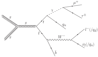
(a)

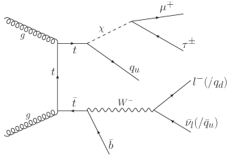
(b)

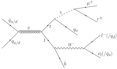
(c)

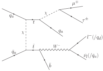
(d)

Figure 1: Feynman diagrams of the signal processes in the DL and SL channels.

What about the size of the off-diagonal Yukawa couplings of $\chi$? The Yukawa couplings when none of the associated quarks is $t$ are set to be vanishingly small. The $\chi tc$ coupling is varied in the range ($0.001-0.01$). This choice is consistent with the observation that $t$ almost invariably decays to $b$ and $W$ with a branching fraction of 0.998 Husemann:2017eka . If we turn on $\chi tu$ at the same time, $D^{0}$–$\bar{D}^{0}$ mixing is triggered through one loop box graph forcing the product of $\chi tc$ and $\chi tu$ couplings to be at most ${10}^{-6}$. The choices are consistent with the ATLAS and CMS searches for rare top decays TopQuarkWorkingGroup:2013hxj ; ATLAS:2015iqc ; CMS:2016uzc ; ATLAS:2017beb ; CMS:2017wcz ; ParticleDataGroup:2018ovx . In our scenario, $\chi$ decays to $\mu$ and $\tau$ with almost 100% branching ratio. As a result, though the exact choice of $\chi\mu\tau$ coupling does not matter much, nevertheless we fix it at $0.01$. The effective signal cross section can be expressed as: $\sigma_{\rm eff}=2\times\sigma(pp\rightarrow t\bar{t})\times{\rm Br}(t\rightarrow bW)\times{\rm Br}(t\rightarrow c\chi)\times{\rm Br}(\chi\rightarrow\mu\tau)\times{\rm Br}(W\rightarrow\ell\nu/jj)$. The overall factor 2 is a combinatoric factor arising from top (anti-top) decay. We summarize our benchmark values in Table. 1.

Parameter	Range
$m_{\chi}\,{\rm(GeV)}$	20, 60, 100
$m_{H}\,{\rm(GeV)}$	200
$Y^{\chi}_{\mu\tau}$	0.01
$Y^{\chi}_{ct}$	0.001 - 0.01

Table 1: Benchmark choices for masses and couplings.

III Collider Analysis

To perform the collider analysis, we first simulate the signal benchmark points (Table 1) and the samples of relevant SM backgrounds (Table 3). After applying a few pre-selection conditions on both signal and background events in order to select coarse signal regions, we proceed to perform MVA techniques. Finally, we estimate the required integrated luminosity to achieve a $5\sigma$ discovery and a $2\sigma$ exclusion. In the following Subsections, we shall present the details of MVA, which are performed to segregate the signal from corresponding backgrounds for each benchmark point.

III.1 Monte Carlo simulation of signal and background processes

We start our analysis by implementing the Yuakawa Lagrangian in FeynRules Alloul:2013bka to generate Universal FeynRules Output (UFO). In the next step, the UFO is interfaced with the event generator to simulate the signal. Both the signal and background events are generated using MadGraph5_aMC@NLO Alwall:2014hca , providing the cross sections at the leading order (LO). For the evaluation of both signal and background cross sections, we employ NN23LO1 as the parton distribution function (PDF) NNPDF:2014otw . The $\tau$ decays are simulated within the TAUOLA package integrated in the MadGraph. These parton level events are then passed through PYTHIA-8 Sjostrand:2014zea for showering and hadronization. To incorporate the detector effects, the resulting events are finally processed through the fast detector simulation package Delphes-3.4.2 deFavereau:2013fsa using the default CMS card. Within Delphes, we use the anti-$k_{T}$ jet clustering algorithm Cacciari:2008gp using the FastJet package Cacciari:2011ma . The respective tagging efficiencies for the $b$ and $\tau$-tagged jets have been parametrically incorporated within the default CMS card.

Among all relevant backgrounds corresponding to two different signal final states SL and DL, the most dominant is the $t\bar{t}$ pair production. This background sample is generated by matching up to two jets. Fully leptonic decays of $t\bar{t}$ pair introduce two leptons in the final state while only one lepton emerges from the semi-leptonic decay of $t\bar{t}$ pair. In addition, associated production of single top with $W$ boson is another significant contributor to the backgrounds. Sizable contributions also arise from $t\bar{t}h$, $t\bar{t}V$, $VV$, and the QCD-QED $b\bar{b}Z^{*}/\gamma^{*}\to b\bar{b}\tau^{+}\tau^{-}$ processes tabulated in Table 3.

III.2 Pre-selection criteria

Relevant acceptance cuts on some of the kinematic variables are required to be applied to identify different particles within the finite size of the detectors. For example, the transverse momentum of each particle ($p_{T}$) should be above a particular threshold to maintain optimum identification efficiency. Rejecting the particles with low $p_{T}$ helps suppress the huge background contributions coming from the QCD processes. Before performing an exhaustive collider analysis, we first apply a set of acceptance cuts (C0) on some of the pertinent kinematic variables as mentioned in Table 2. Although, for signal and for a few background processes (mentioned in Table 3), all these cuts are imposed at the generation level, for some background processes the same cuts are also applied at the analysis level during object selection to keep everything under the same roof. Next, we apply a few more cuts on the lepton and jet multiplicity to achieve the same topology as represented in Figure 1. Below, we describe all the pre-selection cuts (C0 - C5) applied to the signal and background events to select broad signal regions.

• C0 : The acceptance cuts consist of some basic selection criteria for leptons ($e,\mu,\tau$) and jets, imposed on the following set of kinematic variables: $(a)$ transverse momentum $p_{T}$, $(b)$ pseudo-rapidity $\eta$, and $(c)$ angular separation between $i$-th and $j$-th objects $\Delta R_{i,j}$ which is defined in terms of the azimuthal angular separation $(\Delta\phi_{ij})$ and pseudo-rapidity difference $(\Delta\eta_{ij})$ between two objects $i$ and $j$ as $\sqrt{(\Delta\eta_{ij})^{2}+(\Delta\phi_{ij})^{2}}$. The threshold values of these variables are quoted in Table 2.

  Objects	Selection cuts
  $e$	$p_{T}>10$ GeV, $~{}|\eta|<2.5$
  $\mu$	$p_{T}>10$ GeV, $~{}|\eta|<2.4$, $~{}\Delta R_{\mu e}>0.4$
  $\tau_{h}$	$p_{T}>20$ GeV, $~{}|\eta|<2.4$, $~{}\Delta R_{\tau_{h},e/\mu}>0.4$
  $light\,jet$	$p_{T}>20$ GeV, $~{}|\eta|<4.7$, $~{}\Delta R_{{\rm light\,jet},e/\mu}>0.4$
  $b\,jets$	$p_{T}>20$ GeV, $~{}|\eta|<2.5$, $~{}\Delta R_{{\rm b\,jet},e/\mu}>0.4$

  Table 2: Summary of the acceptance cuts.

• C1 : In both DL and SL channels, $\chi$ always decays to $\mu^{\pm}\tau^{\mp}$. But $W$ decays leptonically (hadronically) for the DL (SL) channel. We always identify $\tau$ through its hadronic decay. Thus for the DL channel, final states each with at least one $\mu$ ($e\mu/\mu\mu$) is ensured, whereas for the SL channel, we demand exactly one $\mu$ and no $e$ in the final state.

• C2 : In the final state we require exactly one $\tau$ jet, i.e. $\tau_{h}$, for both the SL and DL channels.

• C3 : One of the pair produced top quarks in the signal decays to $b(\bar{b})W^{-}(W^{+})$ and the other to $\chi$ and a light jet. So, one $b$ tagged jet is required to be present in the final states of both channels. Apart from that, we also apply a cut on the number of light jets. For the DL channel, we demand at least one light jet in the final state, but for the SL analysis, because of the hadronic decay of $W$, the final state consists of minimum three light jets.

• C4 : In the DL channel, the signal topology does not allow for a pair of opposite sign same flavor (OSSF) leptons in the final state arising out of the decay of $Z$-boson. Thus to exclude the $Z$-peak, we veto the events with a pair of OSSF leptons having an invariant mass $M_{\ell^{+}\ell^{-}}$ in the following window: $M_{Z}-10~{}{\rm GeV}\,<\,M_{\ell^{+}\ell^{-}}\,<\,M_{Z}+10$ GeV.

  Process	cross section (pb)	Yields (${\cal L}\,=\,3\,{\rm ab^{-1}}$)
  Signals
  ($m_{\chi},\,Y^{\chi}_{ct}$)	NLO  $[{\rm DL\,||\,SL}]$	DL	SL
  $20,\,0.005$	$0.007\,||\,0.022$	$630$	$2627$
  $20,\,0.01$	$0.028\,||\,0.086$	$2330$	$9385$
  $60,\,0.005$	$0.01\,||\,0.03$	$1977$	$7247$
  $60,\,0.01$	$0.04\,||\,0.12$	$7966$	$28892$
  $100,\,0.005$	$0.006\,||\,0.016$	$1364$	$4778$
  $100,\,0.01$	$0.023\,||\,0.07$	$5312$	$19330$
  SM Backgrounds
  $t\bar{t}\,\to\,2\ell\,+\,jets$	$107.65$ [NNLO]WinNT	$954005.17$	$3891518.73$
  $t\bar{t}\,\to\,1\ell\,+\,jets$	$437.14$ [NNLO]WinNT	$8445.99$	$8709994.85$
  $tW$	$34.81$ [LO]	$2463.11$	$23907.39$
  $Z\,\to\,\tau^{+}\tau^{-}\,+\,jets$	$803$ [NLO]	$419.76$	$20642.35$
  $t\bar{t}(W\,\to\,\ell\nu)\,+\,jets$	$0.25$ [NLO]	$2113.22$	$8566.4$
  $t\bar{t}(W\,\to\,qq)$	$0.103$ (∗) [LO]	$207.74$	$2410.91$
  $t\bar{t}(Z\,\to\,\ell^{+}\ell^{-})\,+\,jets$	$0.24$ [NLO]Kardos:2011na	$4228.31$	$11606.32$
  $t\bar{t}(Z\,\to\,qq)$	$0.206$ (∗) [NLO]Kardos:2011na	$404.22$	$4729.34$
  $WZ\,\to\,3\ell\nu\,+\,jets$	$2.27$ [NLO]Campbell:2011bn	$2404.83$	$2688.63$
  $WZ\,\to\,2\ell\,2q$	$4.504$ [NLO]Campbell:2011bn	$1275.99$	$13659.67$
  $ZZ\,\to\,4\ell$	$0.187$ [NLO]Campbell:2011bn	$169.42$	$95.15$
  $t\bar{t}(h\,\to\,\tau^{+}\,\tau^{-})$	$0.006$ (∗) [LO]	$254.85$	$661.17$
  $b\bar{b}\tau^{+}\tau^{-}$	$0.114$ (∗) [LO]	$36.89$	$728.65$
  $WWW$	$0.236$ [NLO]	$62.0$	$439.92$
  $WWZ$	$0.189$ [NLO]	$47.6$	$510.03$
  $WZZ$	$0.064$ [NLO]	$22.48$	$159.66$
  $ZZZ$	$0.016$ [NLO]	$3.42$	$18.83$
  ${\rm Total~{}background}$		$976565$	$12692338$

  Table 3: Event yields at ${\cal L}\,=\,3\,\rm ab^{-1}$ after applying the pre-selection criteria (C0 - C5) for the analyses in both the DL and SL decay channels.
  ($*$): Some selections are applied at the generation (i.e. Madgraph) level. $p_{T}$ of jets (j) and $b$ quarks (b) $>\,20$ GeV, $p_{T}$ of leptons ($\ell$) $>\,10$ GeV, $|\eta|_{j/b}\,<\,5$, $|\eta|_{\ell}\,<\,2.5$ and $\Delta R_{jj/\ell\ell/j\ell/b\ell}\,>\,0.4$.

• C5 : The next step is to select the leptons and the jets coming from $W$ boson in the DL and SL channels, respectively. As the decay of $\chi$ ensures the presence of one $\mu$, the two possible combinations of leptons in the final state are $\mu\mu$ or $\mu e$ where the second lepton originates from the decay of $W$ in DL channel. While the selection of the $\mu e$ final state is trivial, it is quite challenging to identify the muon is coming from $\chi$ or from $W$. We first check the distribution of $\Delta R$ between $\tau_{h}$ and $\mu$ for the $\mu e$ combination. We observe that in most of the signal events, spatial separation between $\mu$ (coming from $\chi$) and $\tau_{h}$ is smaller than that of $\tau_{h}$ and $e$ originating from $W$. Although this feature is most prominent for the benchmark with the lowest $m_{\chi}$, it persists for the other two benchmarks as well. For the $\mu\mu$ combination as well the same argument holds. First we choose the $\mu$ closer to the $\tau_{h}$. Then we check if the $\mu$ and the $\tau_{h}$ have opposite charges and if it is the case, we consider that $\mu$ to be the decay product of $\chi$. Conversely, if they have same charges, we do not reject the event just on that basis. We check if the $\tau_{h}$ and the distant $\mu$ have opposite charge. If so, we keep that second $\mu$ as the decay product of $\chi$ and the first $\mu$ as the one coming from $W$. This algorithm does not guarantee the selection of the perfect combination, still it makes the selection more efficient. The $\mu$ coming from $\chi$ is denoted by $\mu_{\chi}$ throughout the rest of the discussion.

  For the SL channel, we cannot differentiate whether the jets are coming from $t/\bar{t}$ or from $W$ at first sight. We first compute the invariant mass for each jet pair formed out of all three jets. Then for each event we choose the jet pair having invariant mass closest to $M_{W}$ (within a $30$ GeV window around $M_{W}$), and tag the corresponding jet pair as originated from $W$. From the remaining jets, the leading one is selected as the light jet coming from $t/\bar{t}$. At the end, like in the DL channel, we demand that the $\mu_{\chi}$ and $\tau_{h}$ must have opposite charges.

Apart from the pre-selection conditions, we mention about one particular kinematic variable which turns out to be very important in distinguishing the signal from the backgrounds, namely, the collinear mass of $\mu_{\chi}$-$\tau_{h}$ system, $M_{coll}$. Let us first construct $M_{coll}$ for the two channels. For the DL channel, there are two sources of missing transverse energy $/E_{T}$, i.e. the neutrinos generated in the hadronic decay of $\tau$ and those generated from the leptonic decay of $W$. For SL channel, the single source of $/E_{T}$ is the neutrinos generated from the hadronic decay of $\tau$. Using the collinear approximation ELLIS1988221 for $\tau$ decay, we reconstruct the four momentum of $\tau$. The fundamental assumption is that the decay products of $\tau$ are boosted in the direction of $\tau$ itself since $m_{\tau}\,\ll\,m_{\chi}$. Thus we take the projection of $~{}/E_{T}$ vector along the direction of $\tau_{h}$ which estimates the $p_{T}$ of $\nu_{\tau}$. Then we calculate the four momentum of the actual $\tau$ by modifying the transverse momentum ($p_{T}^{\tau_{h}}$) and energy ($E^{\tau_{h}}$) of the visible decay product $\tau_{h}$ by the factor $\beta\,\equiv\,p_{T}^{\tau_{h}}/(p_{T}^{\tau_{h}}\,+\,p_{T}^{\nu})$. The transverse momentum and energy of the actual $\tau$ can be written as :

$$~{}p_{T}^{\tau}=\frac{p_{T}^{\tau_{h}}}{\beta},~{}E^{\tau}=\frac{E^{\tau_{h}}}{\beta}$$ (1)

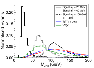
(a) DL

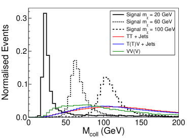
(b) SL

Figure 2: Normalised distributions of collinear mass ($M_{coll}$) for the DL and SL channels.

Although this approximation is not expected to yield the most accurate result for the DL channel because of two different sources for neutrinos, still we construct the collinear mass $M_{coll}$ of the $\mu_{\chi}$-$\tau_{h}$ system using collinear approximation. In Figure 2, we depict the normalised distributions of $M_{coll}$ for both DL and SL channels. For SL channel, the distributions for different benchmarks peak at $m_{\chi}=20$, $60$ and $100$ GeV, respectively. For the DL channel, the corresponding distributions peak around $m_{\chi}$, and not exactly at $m_{\chi}$, for reasons stated above.

A huge number of background events (Table 3) makes it quite challenging to classify the signal events efficiently from the SM backgrounds. Most of the distributions of various kinematic variables are overlapping for signals and backgrounds. So, we avoid the traditional cut based method and deploy several MVA techniques to maximize the sensitivity of the analysis. The cross sections of the signals (scaled at next to leading order by multiplying a $k$-factor of $1.5$ WinNT ) and the SM background along with their yields after the pre-selection at an integrated luminosity $\mathcal{L}\,=\,3\,{\rm ab^{-1}}$ are tabulated in Table 3. Next, we shall briefly describe three different MVA techniques that we employ to maximize the signal significance.

III.3 Multivariate Analysis

Mainly three different MVA techniques, namely, Decorrelated Boosted Decision Tree (BDTD) Roe:2004na , Extreme Gradient Boost (XGBoost) Chen:2016:XST:2939672.2939785 and Deep Neural Network (DNN) lecun2015deep algorithms have been employed to estimate the sensitivity of the signals over the SM backgrounds. For all the three types of MVA techniques, the same set of input variables as mentioned in Table 4 were used. Then we compare the performances of the three methods and use the best one to estimate the signal significance.

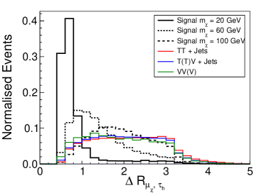
(a)

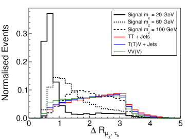
(b)

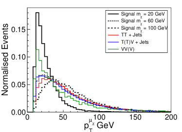
(c)

(d)

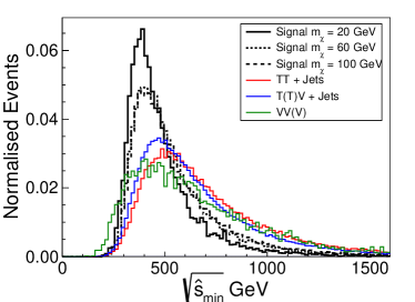
(e)

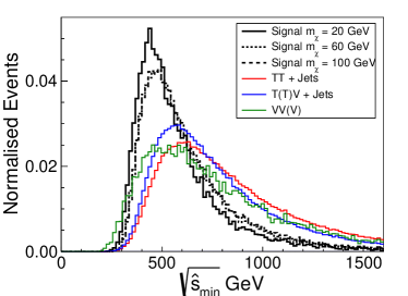
(f)

Figure 3: Distributions of some kinematic variables. Column on the left side is for DL channel and SL channel plots are on the right. The kinematic variables are: (a, b) $\Delta R$ between $\mu_{\chi}$ and $\tau_{h}$, (c, d) $p_{T}$ (in GeV) of $\mu_{\chi}$, and (e, f) $\sqrt{\hat{s}_{min}}$ i.e. minimum parton level center of mass energy.

Among all the input variables used for training the decision trees or neural network, $/E_{T}$, $p_{T}$ of $\mu_{\chi}$ and $\tau_{h}$, $\Delta\phi$ and $\Delta R$ between different final state particles, and the scalar sum of transverse momenta

Variables	Description	DL	SL
$p_{T}^{\tau_{h}},\,\eta^{\tau_{h}}$	$p_{T}$ and $\eta$ of $\tau_{h}$	✓	✓
$p_{T}^{bj},\,\eta^{bj}$	$p_{T}$ and $\eta$ of leading $b$ tagged jet	✓	✓
$/E_{T}$	Missing transverse energy	✓	✓
$p_{T}^{lj}\,\eta^{lj}$	$p_{T}$ and $\eta$ of light jet from $t/\bar{t}$	✓	✓
$p_{T}^{Wj1},\,\eta^{Wj1}$	$p_{T}$ and $\eta$ of leading jet from $W$	✘	✓
$p_{T}^{Wj2},\,\eta^{Wj2}$	$p_{T}$ and $\eta$ of sub leading jet from $W$	✘	✓
$p_{T}^{\mu_{\chi}},\,\eta^{\mu_{\chi}}$	$p_{T}$ and $\eta$ of $\mu$ coming from $\chi$	✓	✓
$p_{T}^{W_{\ell}},\,\eta^{W_{\ell}}$	$p_{T}$ of lepton coming from $W$	✓	✘
$\Delta R_{\mu_{\chi},W_{\ell}}$	$\Delta R$ between leptons coming from $\chi$ and $W$	✓	✘
$\Delta\phi_{\tau_{h},W_{\ell}}$	$\Delta\phi$ between lepton coming from $W$ and $\tau_{h}$	✓	✘
$\Delta\phi_{bj,W_{\ell}}$	$\Delta\phi$ between lepton coming from $W$ and lead $b$ jet	✓	✘
$H_{T}$	Scalar sum $p_{T}$ of all jets	✓	✓
$\Delta R_{\mu_{\chi},\tau_{h}}$	$\Delta R$ between $\mu$ and $\tau_{h}$ coming from $\chi$	✓	✓
$m_{T}^{/E_{T},W_{\ell}}$	$m_{T}$ of lepton from $W$ and $/E_{T}$	✓	✘
$\Delta\phi_{\,/E_{T},\mu_{\chi}}$	$\Delta\phi$ between $/E_{T}$ and the $\mu$ from $\chi$	✓	✓
$\Delta\phi_{\,/E_{T},W_{\ell}}$	$\Delta\phi$ between $/E_{T}$ and the lepton from $W$	✓	✘
$\Delta\phi_{\,/E_{T},bj}$	$\Delta\phi$ between $/E_{T}$ and leading $b$ jet	✘	✓
$\Delta\phi_{\,/E_{T},\tau_{h}}$	$\Delta\phi$ between $/E_{T}$ and $\tau_{h}$	✘	✓
$\Delta R_{Wj1,Wj2}$	$\Delta R$ between the two jets from $W$	✘	✓
$m^{inv}_{\mu,\tau,t_{\ell j}}$	Invariant mass of reconstructed $\tau$, $\mu$ and light jet from $t/\bar{t}$	✘	✓
$\sum\,p_{T}^{all}$	scalar sum $p_{T}$ of all the final state particles	✘	✓
$\Delta\phi_{\,lj,bj}$	$\Delta\phi$ between leading $b$ jet and leading light jet	✓	✓
$\Delta R_{\tau_{h},lj}$	$\Delta R$ between $\tau_{h}$ and leading light jet	✓	✓
$\sqrt{\hat{s}_{min}}$	Minimum parton level center-of-mass energy	✓	✓

Table 4: Some important input variables used(✓) or not(✘), after assessing feature importance Hocker:2007ht ; Breiman2001 , for all of three MVA methods.

of jets $(H_{T})$ turn out to be the most important ones. Figure 3 shows the normalised distributions of a few important kinematic variables for all three signal mass points and the backgrounds. Figures 3a and 3b show the normalised distributions of $\Delta R$ between the $\tau_{h}$ and $\mu$ coming from $\chi$ for DL and SL channels, respectively. The distributions look similar for both the channels as expected. For $m_{\chi}\,=\,20$ GeV, the decay products of $\chi$ are supposed to be more boosted and hence collimated than the other two benchmark points. That is why the distributions with lower $m_{\chi}$ peak at a lower value of $\Delta R$. Next we present the normalised distributions of another important variable $p_{T}$ of $\mu$ coming from $\chi$ for both decay channels in Figure 3c and 3d. The distributions peak towards higher values of $p_{T}$ for higher values of $m_{\chi}$ as expected. we now mention another important variable of importance : minimum parton level centre-of-mass energy i.e. $\sqrt{\hat{s}_{min}}$ Konar:2008ei . This is a global inclusive variable for determining the mass scale of any new physics in the presence of missing energy in the final states. Since the normalised distributions of this variable for signal and backgrounds shown in Figure 3e and 3f are non-overlapping, it has a good discriminating power to identify signals over backgrounds for both the DL and SL channels. We avoid using any kinematic variable related to the reconstructed mass of the yet unseen hypothesized particle to keep aside benchmark dependence. For all the three MVA techniques, $75\%$ of total signal and background events is used for training. Then we evaluate the performances of the respective models using the whole dataset since prior testing on a subset $({\rm remaining}~{}25\%)$ results in negligible over-training.

The entire algorithm of BDTD is executed within the Toolkit for Multivariate Data Analysis (TMVA) framework Hocker:2007ht . Here, Adaptive Boost FREUND1997119 plays a crucial role for robust and efficient classification. To achieve an optimum performance for each benchmark of both the DL and SL channels, we adjust the parameters of BDTD as described in Table 5.

Parameters	Description	Values/Choices
		$m_{\chi}=20$ GeV	$m_{\chi}=60$ GeV	$m_{\chi}=100$ GeV
n_trees	Number of tress	$250$	$250$	$250$
max_depth	Maximum depth of a Decision Tree	$2$	$2$	$2$
boost	Boosting mechanism for training	AdaBoost	AdaBoost	AdaBoost
n_cuts : SL/DL	Number of iteration to find the best split	$50/50$	$46/31$	$45/40$
min_node_size	Minimum events at each final leaf	$2.5\%$	$2.5\%$	$2.5\%$

Table 5: BDTD parameters used for three different mass benchmark points.

XGBoost is another tree based method like BDTD with some additional features. Unlike BDTD, it uses Gradient Boost for classification. To reduce over-training, some additional parameters are used for pruning a decision tree and regularizing the cost function defined as the difference between the true and predicted output – for details on XGBoost see Chen:2016:XST:2939672.2939785 . Table 6 shows the set of XGBoost parameters used for training the signal and background samples.

Parameters	Description	Values/Choices
booster	Tree based learner	$gbtree$
n_estimators	Number of decision trees	$auto$
max_depth	Maximum depth of a Decision Tree	$3$
$\eta$	Learning rate	$0.01$
$\lambda$	Regularization parameter	$0.01$

Table 6: Details of XGBoost parameters.

The third MVA technique that we have employed is Deep Neural Network (DNN). Unlike decision trees, DNN brings in several hidden layers with multiple nodes. Nonlinear activation functions at the nodes help draw nonlinear boundary on the plane of the DNN variables to separate signal from background. The complete DNN training has been performed using keras module of tensorflow-2.3.0 tensorflow2015-whitepaper . All the parameters used for DNN are in Table 7.

Parameters	Description	Values/Choices
n_hidden layers	Number of hidden layers	$5$
n_nodes	Number of neurons in hidden layers	$512$, $256$, $128$, $54$, $8$
activation_func	Function to modify outputs of every nodes	$LeakyRelu$
loss_function	Function to be minimised to get optimum model parameters	$binary\_crossentropy$
optimiser	Perform gradient descent and back propagation	$Adam$ Kingma:2014vow
eta	Learning rate	$0.001$
batch_len	Number of events in each mini batch	$3000$
batch_norm	Normalisation of activation output	$True$
dropout	Fraction of random drop in number of nodes	$20\%$
L2-Regularizer	Regularize loss to prevent overfitting	$0.001$

Table 7: Details of DNN parameters.

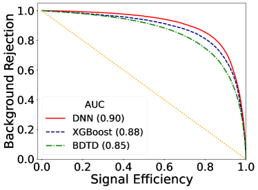
(a) DL ($m_{\chi}~{}=~{}60$ GeV)

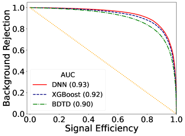
(b) SL ($m_{\chi}~{}=~{}60$ GeV)

Figure 4: ROCs of three MVA techniques for $m_{\chi}\,=\,60$ GeV.

These three MVA techniques discussed above deliver more or less similar performances. In order to compare their responses, we plot the receiver operating characteristic (ROC) curves for all the three methods and compute the area under the curve (AUC) of each ROC in Figure 4. The degree of performance of the MVA techniques increases with increasing AUC. The comparison shows that the DNN performs somewhat better than BDTD and XGBoost in both the DL and SL channels as reflected in Figure 4 for $m_{\chi}\,=\,60$ GeV. The other two choices of $m_{\chi}$ exhibit similar behavior. Next, we shall elaborate the final results only for the DNN technique since it performs the best.

III.4 Results

For evaluation of the signal significance using DNN, we apply suitable cuts on the respective DNN responses that maximize the significance. Then we try to find the required luminosity to achieve a $2\sigma$ exclusion and $5\sigma$ discovery by scanning over $Y^{\chi}_{ct}$. We also estimate the significance after introducing a $5\%$ systematic uncertainty in total number of background events.

Classifiers	Signal efficiency ($\%$)				Maximum significance
	$95$	$80$	$65$	$50$
	Background rejection ($\%$)				${\cal L}=3\,{\rm ab^{-1}}$
BDTD	$49$	$78$	$88$	$93$	$9.34$
XGBoost	$59$	$86$	$92$	$95$	$11.1$
DNN	$64$	$89$	$95$	$97$	$14.9$

Table 8: A quantitative comparison of the three MVA techniques for the DL channel with $m_{\chi}\,=\,60$ GeV and $Y^{\chi}_{ct}\,=\,0.01$.

The benchmark point with $m_{\chi}=20$ GeV still shows a good sensitivity after incorporating a $5\%$ systematic uncertainty in the background. The corresponding sensitivity significantly drops for higher $m_{\chi}$ benchmark points – see Figure 5. Lighter the choice of $\chi$ the more pronounced is the difference in kinematics of the signal compared to the background – a feature observed for all the three MVA techniques.

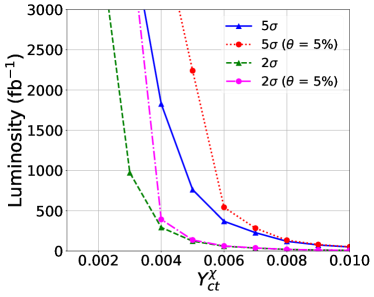
(a) DL : $m_{\chi}\,=\,20$ GeV

(b) SL : $m_{\chi}\,=\,20$ GeV

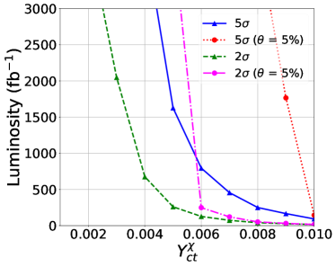
(c) DL : $m_{\chi}\,=\,60$ GeV

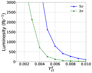
(d) SL : $m_{\chi}\,=\,60$ GeV

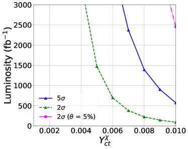
(e) DL : $m_{\chi}\,=\,100$ GeV

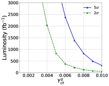
(f) SL : $m_{\chi}\,=\,100$ GeV

Figure 5: Required integrated luminosity to achieve a $2\sigma$ exclusion and $5\sigma$ discovery. The possible systematic uncertainties are expressed through $\theta$.

In Table 8, we have compared the performances of three analysis methods for $m_{\chi}=60$ GeV in the DL channel. We tabulate background rejections for four different signal efficiencies and notice that the DNN is able to reject more background events for a given signal efficiency. In addition, the right most column of Table 8 shows the maximum significance at ${\cal L}=3\,{\rm ab^{-1}}$. Looking at the signal significances one can conclude that the DNN performs somewhat better than the other two methods. This observation is in accordance with the performances based on the previously computed AUCs.

Now we comment on the search prospects of the three benchmark points at the HL-LHC. In Figure 5, we have drawn 2$\sigma$ and 5$\sigma$ contours in the integrated luminosity and $Y^{\chi}_{ct}$ plane with and without considering 5$\%$ linear-in-background systematic uncertainty. In Figure 5a and 5b, for $m_{\chi}=20$ GeV, the 2$\sigma$ and 5$\sigma$ contours drawn with 5$\%$ systematic uncertainty are shifted towards the higher values of $Y^{\chi}_{ct}$, thus requiring more luminosity, for the SL channel relative to the DL channel. Benchmarks with $m_{\chi}=60$ GeV and $m_{\chi}=100$ GeV are accessible to $2\sigma/5\sigma$ significances only with negligible systematic uncertainties. We thus conclude that low $m_{\chi}$ provides promising avenues for exploration both for the DL and SL channels at the HL-LHC. Increasing $m_{\chi}$ lowers the search prospect.

IV Summary and outlook

We have chalked out search strategies for a light exotic pseudoscalar which has only off-diagonal Yukawa interaction with the quarks ($tj$) and leptons ($\mu\tau$). For this, we have focused on the $t\bar{t}$ production and the subsequent decay channels at the 14 TeV HL-LHC with different luminosities. Large accumulation of $t\bar{t}$ events at the HL-LHC will be a gold mine to study such rare top quark decays. We have adopted a simplified scenario with a minor reference to the big picture based on flavor symmetry models that advocate such nonstandard interaction of the exotic spin-0 states.

The present analysis is complementary to a previous study Bhattacharyya:2022ciw where the off-diagonal couplings of the exotic scalar/pseudoscalar were assumed to involve only lighter quarks. The present analysis focuses on off-diagonal Yukawa couplings involving the top quark. It turns out that uncovering the signal processes from the background is more tricky. We have employed three different Machine Learning techniques to perform multivariate analyses and have found that DNN shows somewhat better performance compared to the other two.

We admit that our analysis does not take into consideration some technical nitty-gritties, e.g. jet faking as $\tau_{h}$ and/or leptons, lepton charge misidentification, photon conversions into lepton pairs, uncertainties on luminosity and trigger efficiencies. Once the real data come, the ATLAS and CMS experimentalists are urged to pursue deeper in this direction.

References

- (1) G. Bhattacharyya, S. Dwivedi, D.K. Ghosh, G. Saha and S. Sarkar, Searching for exotic Higgs bosons at the LHC, Phys. Rev. D 106 (2022) 055032 [2202.01068].
- (2) G. Bhattacharyya, P. Leser and H. Pas, Novel signatures of the Higgs sector from S3 flavor symmetry, Phys. Rev. D 86 (2012) 036009 [1206.4202].
- (3) G. Bhattacharyya, P. Leser and H. Pas, Exotic Higgs boson decay modes as a harbinger of flavor symmetry, Phys. Rev. D 83 (2011) 011701 [1006.5597].
- (4) G. Bhattacharyya, I. de Medeiros Varzielas and P. Leser, A common origin of fermion mixing and geometrical CP violation, and its test through Higgs physics at the LHC, Phys. Rev. Lett. 109 (2012) 241603 [1210.0545].
- (5) E. Arganda, X. Marcano, N.I. Mileo, R.A. Morales and A. Szynkman, Model-independent search strategy for the lepton-flavor-violating heavy Higgs boson decay to at the LHC, Eur. Phys. J. C 79 (2019) 738 [1906.08282].
- (6) R.K. Barman, P.S.B. Dev and A. Thapa, Constraining Lepton Flavor Violating Higgs Couplings at the HL-LHC in the Vector Boson Fusion Channel, 2210.16287.
- (7) U. Husemann, Top-Quark Physics: Status and Prospects, Prog. Part. Nucl. Phys. 95 (2017) 48 [1704.01356].
- (8) Top Quark Working Group collaboration, Working Group Report: Top Quark, in Community Summer Study 2013: Snowmass on the Mississippi, 11, 2013 [1311.2028].
- (9) ATLAS collaboration, Search for single top-quark production via flavour-changing neutral currents at 8 TeV with the ATLAS detector, Eur. Phys. J. C 76 (2016) 55 [1509.00294].
- (10) CMS collaboration, Search for anomalous Wtb couplings and flavour-changing neutral currents in t-channel single top quark production in pp collisions at 7 and 8 TeV, JHEP 02 (2017) 028 [1610.03545].
- (11) ATLAS collaboration, Search for flavour-changing neutral current top quark decays in proton-proton collisions at TeV with the ATLAS Detector, .
- (12) CMS collaboration, Search for associated production of a Z boson with a single top quark and for tZ flavour-changing interactions in pp collisions at TeV, JHEP 07 (2017) 003 [1702.01404].
- (13) Particle Data Group collaboration, Review of Particle Physics, Phys. Rev. D 98 (2018) 030001.
- (14) A. Alloul, N.D. Christensen, C. Degrande, C. Duhr and B. Fuks, FeynRules 2.0 - A complete toolbox for tree-level phenomenology, Comput. Phys. Commun. 185 (2014) 2250 [1310.1921].
- (15) J. Alwall, R. Frederix, S. Frixione, V. Hirschi, F. Maltoni, O. Mattelaer et al., The automated computation of tree-level and next-to-leading order differential cross sections, and their matching to parton shower simulations, JHEP 07 (2014) 079 [1405.0301].
- (16) NNPDF collaboration, Parton distributions for the LHC Run II, JHEP 04 (2015) 040 [1410.8849].
- (17) T. Sjöstrand, S. Ask, J.R. Christiansen, R. Corke, N. Desai, P. Ilten et al., An introduction to PYTHIA 8.2, Comput. Phys. Commun. 191 (2015) 159 [1410.3012].
- (18) DELPHES 3 collaboration, DELPHES 3, A modular framework for fast simulation of a generic collider experiment, JHEP 02 (2014) 057 [1307.6346].
- (19) M. Cacciari, G.P. Salam and G. Soyez, The anti- jet clustering algorithm, JHEP 04 (2008) 063 [0802.1189].
- (20) M. Cacciari, G.P. Salam and G. Soyez, FastJet User Manual, Eur. Phys. J. C 72 (2012) 1896 [1111.6097].
- (21) “Nnlo+nnll top-quark-pair cross sections.” https://twiki.cern.ch/twiki/bin/view/LHCPhysics/TtbarNNLO.
- (22) A. Kardos, Z. Trocsanyi and C. Papadopoulos, Top quark pair production in association with a Z-boson at NLO accuracy, Phys. Rev. D 85 (2012) 054015 [1111.0610].
- (23) J.M. Campbell, R.K. Ellis and C. Williams, Vector boson pair production at the LHC, JHEP 07 (2011) 018 [1105.0020].
- (24) R. Ellis, I. Hinchliffe, M. Soldate and J. Van Der Bij, Higgs decay to a possible signature of intermediate mass higgs bosons at high energy hadron colliders, Nuclear Physics B 297 (1988) 221.
- (25) B.P. Roe, H.-J. Yang, J. Zhu, Y. Liu, I. Stancu and G. McGregor, Boosted decision trees, an alternative to artificial neural networks, Nucl. Instrum. Meth. A 543 (2005) 577 [physics/0408124].
- (26) T. Chen and C. Guestrin, XGBoost: A scalable tree boosting system, in Proceedings of the 22nd ACM SIGKDD International Conference on Knowledge Discovery and Data Mining, KDD ’16, (New York, NY, USA), pp. 785–794, ACM, 2016, DOI.
- (27) Y. LeCun, Y. Bengio and G. Hinton, Deep learning, nature 521 (2015) 436.
- (28) A. Hocker et al., TMVA - Toolkit for Multivariate Data Analysis, physics/0703039.
- (29) L. Breiman, Random forests, Machine Learning 45 (2001) 5.
- (30) P. Konar, K. Kong and K.T. Matchev, : A Global inclusive variable for determining the mass scale of new physics in events with missing energy at hadron colliders, JHEP 03 (2009) 085 [0812.1042].
- (31) Y. Freund and R.E. Schapire, A decision-theoretic generalization of on-line learning and an application to boosting, Journal of Computer and System Sciences 55 (1997) 119.
- (32) M. Abadi, A. Agarwal, P. Barham, E. Brevdo, Z. Chen, C. Citro et al., TensorFlow: Large-scale machine learning on heterogeneous systems, 2015.
- (33) D.P. Kingma and J. Ba, Adam: A Method for Stochastic Optimization, 12, 2014 [1412.6980].
- (34) G. Cowan, K. Cranmer, E. Gross and O. Vitells, Asymptotic formulae for likelihood-based tests of new physics, Eur. Phys. J. C 71 (2011) 1554 [1007.1727].