Marginal-Certainty-aware Fair Ranking Algorithm

Abstract.

Ranking systems are ubiquitous in modern Internet services, including online marketplaces, social media, and search engines. Traditionally, ranking systems only focus on how to get better relevance estimation. When relevance estimation is available, they usually adopt a user-centric optimization strategy where ranked lists are generated by sorting items according to their estimated relevance. However, such user-centric optimization ignores the fact that item providers also draw utility from ranking systems. It has been shown in existing research that such user-centric optimization will cause much unfairness to item providers, followed by unfair opportunities and unfair economic gains for item providers.

To address ranking fairness, many fair ranking methods have been proposed. However, as we show in this paper, these methods could be suboptimal as they directly rely on the relevance estimation without being aware of the uncertainty (i.e., variance of the estimated relevance). To address this uncertainty, we propose a novel Marginal-Certainty-aware Fair algorithm named MCFair. MCFair jointly optimizes fairness and user utility, while relevance estimation is constantly updated in an online manner. In MCFair, we first develop a ranking objective that includes uncertainty, fairness, and user utility. Then we directly use the gradient of the ranking objective as the ranking score. We theoretically prove that MCFair based on gradients is optimal for the aforementioned ranking objective. Empirically, we find that on semi-synthesized datasets, MCFair is effective and practical and can deliver superior performance compared to state-of-the-art fair ranking methods. To facilitate reproducibility, we release our code.

1. INTRODUCTION

Advanced ranking techniques have led to improvements in AI-powered information services that significantly changed people’s lives. For example, search engines that rank documents according to their utilities to user’s queries have helped billions of people better finish their daily work; recommendation systems that rank products/movies/news according to the user’s interests have completely changed the way people obtain information every day. Therefore, how to construct and optimize ranking systems is one of the crucial research problems in Information Retrieval (IR) (Liu et al., 2009).

When considering the quality of result rankings in a ranking system, there are two important criteria: Ranking Effectiveness and Ranking Fairness (Morik et al., 2020; Singh and Joachims, 2018; Biega et al., 2018). Ranking Effectiveness refers to the ability of a ranking system to effectively put relevant results at the top ranks; by maximizing ranking effectiveness, we can help save users’ efforts as they only need to examine the top ranks to satisfy their information needs (Wang et al., 2018; Joachims et al., 2017). However, myopically optimizing ranking effectiveness according to relevance can lead to unfair ranking results. For example, in a hiring website, if a ranking system only considers ranking effectiveness and ranks candidates solely according to relevance, then a small number of top candidates will always be exposed to employers and dominate employers’ attention as employers usually only examine the top ranks (Joachims et al., 2017). In this case, other candidates will be unfairly treated and rarely have the chance to be hired even when they are also highly qualified for the job. Therefore, it is critical to jointly consider ranking fairness and ranking effectiveness. Formally, ranking fairness measures the ranking system’s ability to present fairly (Singh and Joachims, 2018). In this work, we focus on the important problem of Exposure Fairness, as exposure directly influences opinion (e.g., ideological orientation of presented news articles) or economic gain (e.g., revenue from product sales or streaming) for providers of items (Morik et al., 2020).

Relevance estimation serves as the foundation of the optimization of effectiveness and fairness. Specifically, optimizing effectiveness means putting more relevant items on top ranks, while optimizing fairness means letting items of similar relevance receive similar exposure. To jointly optimize ranking effectiveness and fairness, many fair ranking methods (Singh and Joachims, 2018; Biega et al., 2018; Yang et al., 2022b) adopt a post-processing setting that assumes that relevance is well estimated prior to the effectiveness-fairness joint optimization. However, such a post-processing setting seldom exists. In a real-world scenario, relevance estimation and ranking optimization are usually dynamically entangled with each other in an online way. Relevance estimation influences how the ranked lists are optimized, and the ranked lists will be later presented to users to collect their feedback, which will, in return, influence relevance estimation. From a statistical point of view, relevance estimation usually comes with uncertainty, i.e., variance and relevance estimations for different items are not equally trustworthy since their uncertainty is usually not the same. Optimizing ranking effectiveness and fairness without considering such differences in uncertainty will make existing post-processing fair methods suboptimal. It has come to our notice that although some methods (Morik et al., 2020; Yang and Ai, 2021) have been proposed to balance ranking effectiveness and fairness in an online setting, these methods overlook the uncertainty difference in relevance estimation. In this paper, we will show these uncertainty-oblivious ranking methods are suboptimal in the online setting.

In this paper, we propose a Marginal-Certainty-aware Fair ranking algorithm, or MCFair to jointly optimize effectiveness and fairness in an online setting. This algorithm addresses the dynamic nature of online setting where rank optimization is carried out while the relevance is still being learnt from users’ biased feedback. The core of our algorithm is to first formulate a ranking objective that includes effectiveness, fairness, and uncertainty, then take derivatives of the ranking objective with respect to exposure and directly use the gradients as ranking scores. The ranking scores from the gradients automatically include a marginal-certainty-aware exploration strategy to deal with the uncertainty in relevance estimation. We theoretically prove that the ranking scores, i.e., gradients, are optimal for the ranking objective. In addition to the theoretical justification of MCFair, we provide empirical results with two real-world datasets under both the post-processing setting and the online setting. We find that MCFair outperforms existing state-of-the-art methods significantly. Furthermore, MCFair is efficient, robust, and easy to implement.

2. RELATED WORK

Exposure Fairness in Ranking. Fairness has been a heated research topic in the IR community, especially in ranking (Zehlike et al., 2017, 2022; Zehlike and Castillo, 2020; Oosterhuis and de Rijke, 2020; Morik et al., 2020), There exist various definitions and criteria of ranking fairness (Mehrabi et al., 2021; Singh et al., 2021). In this work, we specifically focus on Exposure Fairness, which is crucial for ranking services. For exposure fairness, Biega et al. (2018) and Singh and Joachims (2018) independently propose the well-known amortized fairness principle where items’ exposure should be proportional to their relevance. Some prior works (Yang and Ai, 2021; Yang et al., 2022b; Biega et al., 2018; Singh and Joachims, 2018, 2019; Morik et al., 2020; Wu et al., 2021; Oosterhuis, 2021) have been proposed to address the amortized fairness. Among these works, (Yang and Ai, 2021; Morik et al., 2020) choose to first identify unfairly-treated items based on some predefined metrics, then boost these items’ ranking scores to gain more exposure and mitigate existing unfairness. However, these methods based on predefined metrics could be suboptimal because they don’t directly optimize fairness (more discussion in §4.1). Another line of works (Biega et al., 2018; Singh and Joachims, 2018) proposes to use linear programming (LP) methods to directly optimize fairness. However, the number of decision variables of these LP methods is $O(n^{2})$, which quadratically increases when the number of candidate items n increases. This $n$ can be a huge number in real-world ranking applications, and $O(n^{2})$ decision variables become the bottleneck of the LP methods.

Uncertainty in Ranking. Model Uncertainty has been widely studied in ML and Statistics community (Draper, 1995; Gal and Ghahramani, 2016). In IR literature, Zhu et al. (Zhu et al., 2009) propose to improve retrieval performance by utilizing the variance of a probabilistic language model as the risk-based factor. Some other works also make use of model uncertainty to improve query performance prediction (Roitman et al., 2017; Schuth et al., 2015), query cutoff prediction (Culpepper et al., 2016; Lien et al., 2019) as well as neural IR (Penha and Hauff, 2021; Cohen et al., 2021). However, the exploration of uncertainty in learning to rank has become popular recently. For example, Singh et al. (2021) proposed a new type of ranking fairness based on uncertainty. A most recent work from Yang et al. (2022a) proposes to use uncertainty to explore cold-start items in online ranking services. In this paper, unlike previous works which use uncertainty directly, we propose to use marginal (un)certainty to guide exploration.

Unbiased and Online LTR. Unbiased learning to rank focuses on training unbiased models with biased click signals (Ai et al., 2018b, 2021; Joachims et al., 2017), which have been a heated topic in recent years (Tran et al., 2022; Zhao et al., 2022). Offline LTR trains the unbiased model with offline click logs (Ai et al., 2018a; Joachims et al., 2017; Oosterhuis and de Rijke, 2021; Luo et al., 2022; Tran et al., 2021; Yang et al., 2020) while online LTR focuses on actively removing biases from labels via online interpolations (Yang et al., 2022a; Hofmann et al., 2013). Within online LTR, some works propose to explore the relevance of result rankings with bandit learning (Schuth et al., 2016; Wang et al., 2019; Yue and Joachims, 2009; Xu et al., 2022); Oosterhuis and de Rijke (2020) propose to dynamically estimate items’ relevance via stochastic ranking sampling. Yang et al. (2022a) analyze the effect of using behavior features (click data) as both features and labels for online LTR. However, most of the existing unbiased and online LTR methods only focus on estimating relevance and maximizing effectiveness. In this paper, following (Morik et al., 2020), we will explore an algorithm to jointly optimize ranking effectiveness (relevance) and fairness.

3. BACKGROUND

In this section, we give the background knowledge for this paper, which includes the workflow of ranking service (§1), metrics for ranking optimization (§3.2) and biased user feedback in ranking service (§3.3). A summary of notations is shown in Table 1.

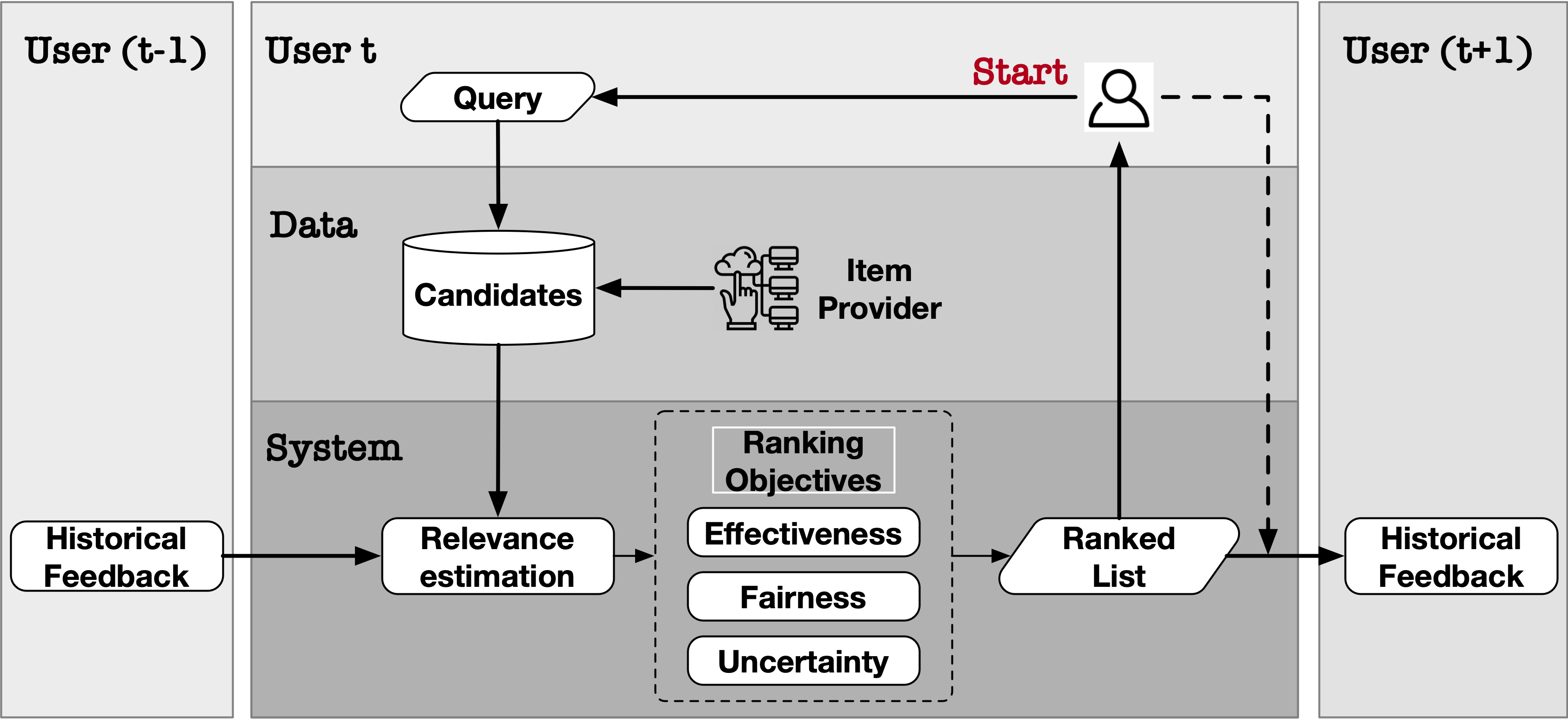
Figure 1. Workflow of ranking services.

3.1. The Workflow of Ranking Service

Table 1. A summary of notations.

$d,q,D(q)$	For a query $q$, $D(q)$ is the set of candidates items. $d\in D(q)$ is an item.
$e,r,c$	All are binary random variables indicating whether an item $d$ is examined ($e=1$), perceived as relevant ($r=1$) and clicked ($c=1$) by a user respectively.
$R,p_{i},E,\pi$	$R=p(r=1|d)$, is the probability of an item $d$ perceived as relevant. $p_{i}=p(e=1|rnk(d)=i,\pi)$ is the examination probability of item $d$ when it is put in $i^{th}$ rank in a ranklist $\pi$. $E$ is item’s accumulated examination probability (see Eq.7).
$k_{s},k_{c}$	Users will stop examining items lower than rank $k_{s}$ due to selection bias (see Eq. 11). $k_{c}$ is the cutoff prefix to evaluate cNDCG and $k_{c}\leq k_{s}$.

Here we introduce the workflow of ranking service in detail. Figure 1 is the flowchart of a ranking task. At time step $t$, a user issues a query, and there are several candidate items corresponding to this query. Then the relevance estimator predicts the relevance of each candidate item and the ranking optimization methods will generate the ranked list by optimizing the ranking objective based on relevance estimation. There are a few different ranking objectives can be adopted here. For example, the ranking objective can be to jointly optimize effectiveness and fairness (Yang et al., 2022b). After examining the ranked list, the user will provide their feedback, such as clicks. With user’s feedback, the relevance estimator will update relevance estimation for future ranking optimization. The generated ranked list will be evaluated by the ranking utility measurement.

3.2. Ranking Utility Measurement

Ranking is a two-sided market, from which users and item providers both draw utility. Here we introduce the concepts of user-side utility and provider-side utility, which provide guidance on how we optimize and evaluate ranked lists.

3.2.1. The User-side Utility (Effectiveness).

Before introducing the user-side utility, we define the relevance $R(d,q)$ in this paper as the probability of an item $d$ to be relevant to query $q$:

(1) $$\vspace{0pt}R(d,q)=P(r=1|d,q)\vspace{0pt}$$

where $r$ is a binary random variable indicating $d$ perceived by a user as relevant to query $q$ or not.

As users are the main clients of ranking systems, it is important to evaluate ranking performance from the user side. The user-side utility, also referred to as effectiveness, is usually used to measure a ranking system’s ability to put relevant items on top ranks. One widely-used user-side utility measurement is Discounted Cumulative Gain (Järvelin and Kekäläinen, 2002), denoted as DCG. For a ranked list $\pi$ corresponding to a query $q$, we define $\textit{DCG}@k_{c}$ as:

(2) $$\vspace{0pt}\textit{DCG}@k_{c}(\pi)=\sum_{i=1}^{k_{c}}R(\pi[i],q)\lambda_{i}\vspace{0pt}$$

where $\pi[i]$ indicates the $i^{th}$ ranked item in the ranked list $\pi$; $R(\pi[i],q)$ indicates item $\pi[i]$’s relevance to query $q$; cutoff $k_{c}$ indicates the top ranks we evaluate; $\lambda_{i}$ indicates the weight we put on $i^{th}$ rank. $\lambda_{i}$ usually monotonically decreases as rank $i$ increases since top ranks are generally more important. For example, $\lambda_{i}$ is sometimes set to $\frac{1}{\log_{2}(i+1)}$. In this paper, we follow (Singh and Joachims, 2018) and set $\lambda$ as the examining probability $p$:

(3) $$\vspace{0pt}\textit{DCG}@k_{c}(\pi)=\sum_{i=1}^{k_{c}}R(\pi[i],q)\cdot p_{i}\vspace{0pt}$$

where $p_{i}$ is users’ examining probability of the $i^{th}$ item in ranked list $\pi$, and we have:

(4) $$\vspace{0pt}p_{i}=P(e_{i}=1)$$

where $e_{i}$ is a binary variable indicating the $i^{th}$ item being examined or not. Then, we can define the normalized-DCG (NDCG) by normalizing $\textit{DCG}@k_{c}(\pi)$ with $\textit{DCG}@k_{c}(\pi^{*})$:

(5) $$\vspace{0pt}\textit{NDCG}@k_{c}(\pi)=\frac{\textit{DCG}@k_{c}(\pi)}{\textit{DCG}@k_{c}(\pi^{*})}\vspace{0pt}$$

where $\pi^{*}$ is the ideal ranked list constructed by arranging items by their true relevances and $\textit{NDCG}@k_{c}(\pi)\in[0,1]$. Furthermore, we could define Cumulative NDCG (cNDCG) as:

(6) $$\vspace{0pt}\begin{split}\textit{eff.}=\textit{cNDCG}@k_{c}=\sum_{\tau=1}^{t}\gamma^{t-\tau}\textit{NDCG}@k_{c}(\pi_{\tau})\end{split}\vspace{0pt}$$

where $0\leq\gamma\leq 1$ is the discounted factor, $t$ is the current time step. Note that $\gamma$ is usually set as a constant for all time steps. Compared to NDCG, cNDCG can better evaluate effectiveness for online ranking services  (Schuth et al., 2013). Since we mainly consider online ranking (as shown in Figure 1), we use cNDCG as the effectiveness objective and measurement in this work.

3.2.2. The Provider-side Utility (Fairness).

Since items’ rankings can determine their providers’ utility, it is also important to evaluate ranking performance from the provider perspective. In the literature, Provider-side Utility is used to measure a ranking system’s ability to create a fair environment for items and their providers. Since a fair environment should let similar items be treated similarly, items of similar relevance should get similar exposure in this fair ranking system, i.e., the amortized fairness principle (Singh and Joachims, 2018; Biega et al., 2018). Following existing works (Singh and Joachims, 2018; Biega et al., 2018; Yang and Ai, 2021; Singh and Joachims, 2019), item $d$’s exposure is defined as its accumulated examination probability:

(7) $$\vspace{0pt}\begin{split}E(d)&=\sum_{i=1}^{t}\sum_{j=1}^{k}p_{j}\mathbbm{1}_{\pi_{i}[j]==d}\end{split}\vspace{0pt}$$

where $\pi_{i}[j]$ indicates the $j^{th}$ item in ranked list $\pi_{i}$, $\mathbbm{1}$ is the indicator function which indicates that $p_{j}$ will contribute $E(d)$ only when $\pi_{i}[j]$ is item $d$. With items’ exposure, we follow (Oosterhuis, 2021) to define the unfairness as:

(8) $$\begin{split}\textit{unfairness}&=\frac{1}{n(n-1)}\sum_{d_{x}\in D(q)}\sum_{d_{y}\in D(q)}\bigg{(}E(d_{x})R(d_{y})-E(d_{y})R(d_{x})\bigg{)}^{2}\\ \textit{fairness}&=-\textit{unfairness}\vspace{0pt}\end{split}$$

where $D(q)$ is the set of candidate items for query $q$. This unfairness measures the average exposure disparity between item pairs, and the fairness is just the negative of unfairness. Besides, we use $R$ or $R(d)$ as $R(d,q)$ for simpler notation in later formulation.

3.3. Partial and Biased Feedback

As shown in the ranking service’s workflow in Figure 1, we rely on users’ feedback to update the relevance estimation. However, users’ feedback could be partial and biased indicator of relevance since users only provide meaningful feedback for items that they have examined, we have:

(9) $$\vspace{0pt}c=\begin{cases}r,&\text{if}\quad e=1\\ 0,&\textit{otherwise}\end{cases}\vspace{0pt}$$

where binary random variable $e$ indicates whether an item has been examined by the user or not; binary random variable $r$ indicates whether an item is perceived as relevant by the user; binary random variable $c$ indicates whether an item is clicked by the user. Following existing works on click model (Chuklin et al., 2015; Yang and Ai, 2021), we model the probability of click $c$ as:

(10) $$\vspace{0pt}p(c=1)=p(r=1)p(e=1)\vspace{0pt}$$

where $p(e=1)$ is users’ examination probability. Following existing works(Oosterhuis and de Rijke, 2021; Yang et al., 2022a), we assume two kinds of biases exist in examination probability.

Positional Bias (Craswell et al., 2008; Joachims et al., 2017): The examination probability drops along ranks (also called position), and we model it with $p(rank(d|\pi))$, where the examining probability only depends on the rank.

Selection Bias (Oosterhuis and de Rijke, 2021, 2020): This bias exists when not all of the items are selected to be shown to users or some lists are so long that no user will examine the entire lists. We model this by assuming that items ranked lower than rank $k_{s}$ won’t be examined by the user:

(11) $$\vspace{0pt}P(e=1|d,\pi)=\begin{cases}p(\textit{rank}(d|\pi)),&\text{if}\quad\textit{rank}(d|\pi)\leq k_{s}\\ 0,&\textit{otherwise}\end{cases}$$

4. PROPOSED METHOD

The challenge of optimizing fairness and effectiveness lies in the fact that the ranking optimization is being carried out based on relevance estimation while relevance estimation is still being learned. From a statistical point of view, an estimation such as relevance estimation mostly contains uncertainty, i.e., variance, and possibly some bias, which can make the optimization of fairness and effectiveness suboptimal. For example, an item with under-estimated relevance and high uncertainty might never get presented to users since both optimizing fairness and optimizing effectiveness will rank irrelevant items to the lower positions of the ranked lists. No presentation will make this item hard to collect feedback to effectively update its relevance estimation. However, this item might be actually relevant and we will know its relevance if more user feedbacks are collected to reduce the uncertainty in its relevance estimation. Although many existing methods can give an unbiased estimation of relevance (Oosterhuis and de Rijke, 2021; Yang et al., 2022a), the uncertainty (i.e., variance) in this estimation might still make the relevance estimation unreliable, which will make them deliver suboptimal ranking results. To address uncertainty, we propose a Marginal-Certainty-aware Fair ranking algorithm called MCFair, which jointly optimizes effectiveness and fairness.

For the rest of this section, we first propose a gradient-based ranking optimization framework to optimize fairness and effectiveness where we assume uncertainty does not exist (§4.1); then we further extend this framework to be uncertainty-aware (§4.2). Finally, we introduce the specific relevance estimator used for the proposed framework (§4.3).

4.1. Gradient-based Optimization Framework

In this section, we introduce a gradient-based ranking optimization framework. As shown in Figure 1, at time step $t$, one user issues a query $q$ and the objective of the framework is to find the optimum ranked list $\pi_{t}$ that jointly maximizes effectiveness and fairness:

(12) $$\max_{\pi_{t}}\quad\textit{Obj.}(q,t)=\textit{eff.}(q,t)+\alpha\textit{fair.}(q,t)$$

where $\alpha$ is the coefficient to balance the two utility. In this ranking objective, according to Eq. 5 and Eq. 6, we can reorganize the effectiveness as:

(13) $$\vspace{0pt}\textit{eff.}(q,t)=\textit{cNDCG}@k_{s}=\frac{1}{\textit{DCG}@k_{s}(\pi^{*})}\sum_{\tau=1}^{t}\gamma^{t-\tau}\textit{DCG}@k_{s}(\pi_{\tau})\vspace{0pt}$$

In this paper, we will adopt $k_{s}$ (defined in Eq. 11) as the cutoff for ranking effectiveness optimization unless explicitly specified. Besides the cutoff, we will set $\gamma=1$ in Eq. 13 for simplicity, and we will relax it to all $\gamma$ within $[0,1]$ in later discussion. By ignoring the constant $\textit{DCG}@k_{s}(\pi^{*})$, we can get the eff. as:

(14) $$\begin{split}\textit{eff.}(q,t)&=\textit{cNDCG}@k_{s}=\sum_{\tau=1}^{t}\textit{DCG}@k_{s}(\pi_{\tau})=\sum_{i=1}^{t}\sum_{j=1}^{k}p_{j}R(\pi_{i}[j])\\ &=\sum_{d\in D(q)}\big{(}\smash[lr]{\sum_{i=1}^{t}\sum_{j=1}^{k}p_{j}R(d)\mathbbm{1}_{\pi_{i}[j]==d}\big{)}}\\ &=\sum_{d\in D(q)}R(d)\big{(}\sum_{i=1}^{t}\sum_{j=1}^{k}p_{j}\mathbbm{1}_{\pi_{i}[j]==d}\big{)}\\ &=\sum_{d\in D(q)}R(d)E(d)\end{split}$$

where $p_{j}$ is the examination probability of $j^{th}$ rank and $\pi_{i}[j]$ indicates the $j^{th}$ item in user $i$’s ranked list $\pi_{i}$. $E(d)$ is the cumulative exposure defined Eq. 7. The above effectiveness formulation means that we should allocate more exposure $E(d)$ to items with greater relevance $R(d)$.

At time step $t$, the optimization goal defined in Eq. 12 is actually equivalent to finding $\pi_{t}$ to maximize the marginal objective, denoted as $\Delta\textit{Obj.}(q,t)$:

(15) $$\begin{split}\max_{\pi_{t}}\;\textit{Obj.}(q,t)&\equiv\max_{\pi_{t}}\quad\textit{Obj.}(q,t)-\textit{Obj.}(q,t-1)\\ &=\max_{\pi_{t}}\quad\Delta\textit{Obj.}(q,t)\\ &=\max_{\pi_{t}}\quad\Delta\textit{eff.}(q,t)+\alpha\Delta\textit{fair.}(q,t)\end{split}$$

where the marginal objective is the increment of objective at time step $t$. $\equiv$ means equivalence. The equivalence is due to the fact that the ranked list $\pi_{t}$ at time step $t$ won’t change $\textit{Obj.}(t-1)$ because $\pi_{t}$ cannot change history.

To optimize $\Delta\textit{Obj.}(q,t)$, we take the first order approximation of the above marginal objective $\Delta\textit{Obj.}(q,t)$ by considering marginal exposure $\Delta E$’s influence:

(16) $$\begin{split}\quad&\Delta\textit{Obj.}(q,t)\approx\sum_{d\in D(q)}\frac{\partial{\textit{eff.}}}{\partial E(d)}\Delta E(d)+\alpha\sum_{d\in D(q)}\frac{\partial{\textit{fair.}}}{\partial E(d)}\Delta E(d)\\ &=\sum_{d\in D(q)}R(d)\Delta E(d)\\ +&\alpha\sum_{d\in D(q)}\underbrace{\frac{4}{n(n-1)}\bigg{(}R(d)\sum_{l}E(l)R(l)-E(d)\sum_{h}R^{2}(h)\bigg{)}}_{\text{B(d)}}\Delta E(d)\\ &=\sum_{d\in D(q)}\underbrace{(R(d)+\alpha B(d))}_{g(d)}\Delta E(d)=\langle\vec{g}\;,\;\Delta\vec{E}\rangle\end{split}$$

where $\vec{g}$ is $[g(d)\>\forall d\in D(q)]$, the vector form of gradients, $\langle,\rangle$ denotes dot product. The marginal objective at time step $t$ can be approximated by the dot product of gradient $\vec{g}$ and marginal exposure $\Delta\vec{E}$ at time step $t$, i.e. $\langle\vec{g}\;,\;\Delta\vec{E}\rangle$. Actually, the gradient of effectiveness is $R(d)$, regardless of whether $\gamma=1$ or $0\leq\gamma\leq 1$, since $\gamma$ only affect how we weight the historical DCGs (see Eq. 13) in effectiveness and historical DCGs will not affect the current DCG at time step $t$, i.e., the marginal effectiveness. So, the above derivation still holds when $0\leq\gamma\leq 1$. The marginal exposure $\Delta\vec{E}$ is the exposure each item will get at time step $t$, i.e., $p_{j}$ in Eq. 14. Since $p_{j}\in(0,1)$ is relatively small, the objective’s first-order approximation should approximate $\Delta\textit{Obj.}(q,t)$ well. Furthermore, we can reformulate $\Delta\textit{Obj.}(q,t)$ as:

(17) $$\begin{split}\quad\Delta\textit{Obj.}(q,t)&\approx\sum_{d\in D(q)}g(d)\Delta E(d)=\sum_{k=1}^{|D(q)|}g(\pi_{t}[k])p_{k}\end{split}$$

where $\pi_{t}[k]$ is the $k^{th}$ item in the ranklist $\pi_{t}$. To maximize the above $\Delta\textit{Obj.}(q,t)$, we first introduce the Rearrangement Inequality (refer to Section 10.2, Theorem 368 in (Hardy et al., 1952)).

Lemma 4.1.

Given $0\leq x_{1}\leq x_{2}\leq...\leq x_{n}$ and $y_{1}\leq y_{2}\leq...\leq y_{n}$, we have:

(18) $$\sum_{i=1}^{n}x_{\sigma(i)}y_{i}\leq\sum_{i=1}^{n}x_{i}y_{i}\vspace{0pt}$$

where $\sigma$ can be any possible permutation.

According to the above rearrangement inequality, we should let item with greater gradient $g(d)$ get greater examination probability $p_{k}$ in order to maximize $\Delta\textit{Obj.}(q,t)$. By assuming that $p_{k}$ drops as rank $k$ increases, we can maximize $\Delta\textit{Obj.}(q,t)$ by generating a ranked list $\pi_{t}$ that arranges items according to their gradients $g$ in descending order:

(19) $$\pi_{t}=\arg_{\textit{topk}}\big{(}g(d)|\forall d\in D(q)\big{)}$$

where $k$ is the length of ranked list $\pi_{t}$.

Aside from optimization, in this paper, we also reveal an interesting relation between effectiveness and fairness. When fairness constraint is strictly satisfied and unfairness is reduced to zero, $\textit{cNDCG}@k_{s}$ is actually fixed. Then, according to Eq. 8, we can reduce the unfairness to zero when items get exposure as:

(20) $$\vspace{0pt}\bar{E}(d)=\frac{R(d)}{\sum_{h\in D}R(h)}E_{sum}\quad\forall d\in D(q)\vspace{0pt}$$

where the total exposure $E_{sum}=\sum_{d\in D}E(d)$. By setting ${E}(d)$ to $\bar{E}(d)$ in Eq. 14, we can get the $\textit{cNDCG}@k_{s}$ as:

(21) $$\vspace{0pt}\begin{split}\overline{cNDCG}@k_{s}&=\sum_{d\in D(q)}R(d)E(d)=\frac{\sum_{d\in D(q)}R^{2}(d)}{\sum_{h\in D}R(h)}E_{\textit{sum}}\end{split}\vspace{0pt}$$

where we still assume $\gamma=1$ and ignore the normalization. From the above derivation, we could know that $\textit{cNDCG}@k_{s}$ is fixed as long as the fairness constraint is strictly satisfied, no matter which algorithm we use to reach fairness. Although $\textit{cNDCG}@k_{s}$ is fixed, it still leaves us much freedom to improve the top ranks’ effectiveness $\textit{cNDCG}@k_{c}$ ($k_{c}<k_{s}$) as well as to improve effectiveness when some tolerance of fairness is allowed.

4.2. Uncertainty-aware Ranking Optimization

In this section, we will extend the above gradient-based ranking optimization framework to be uncertainty-aware.

In the above ranking optimization, we optimize ranking in a post-processing setting where relevance $R$ is already well-estimated prior to ranking optimization, and we can calculate $g$ in Eq. 16 as the ranking score based on the pre-estimated relevance. Such an assumption means we optimize ranking in a post-processing manner. However, in real-world applications, relevance estimation and ranking optimization are often entangled in an online setting, where ranking optimization takes place while relevance estimation is still being learned. The online setting brings us a problem relevance estimation is often not perfect and contains uncertainty (variance). In this section, we focus on the scenario where relevance is estimated online with uncertainty.

To analyze uncertainty, we first accumulate the uncertainty of all candidate items:

(22) $$\savestack{\tmpbox}{\stretchto{\scaleto{\scalerel*[width("\textit{uncert.}")]{\kern-0.6pt\bigwedge\kern-0.6pt}{\rule[-505.89pt]{4.30554pt}{505.89pt}}}{}}{0.5ex}}\stackon[1pt]{\textit{uncert.}}{\tmpbox}(q,t)=\sum_{d\in D(q)}\textit{Variance}(\hat{R}(d))$$

where $\hat{R}(d)$ is item $d$’s relevance estimation and $\textit{Variance}(\hat{R}(d))$ is the variance of $\hat{R}(d)$; we leave co-variance to future work. As for how to estimate relevance, we will discuss it in §4.3. Being uncertainty-aware, we formulate the ranking objective as:

(23) $$\max_{\pi_{t}}\quad\textit{Obj.}(q,t)=\savestack{\tmpbox}{\stretchto{\scaleto{\scalerel*[width("\textit{eff.}")]{\kern-0.6pt\bigwedge\kern-0.6pt}{\rule[-505.89pt]{4.30554pt}{505.89pt}}}{}}{0.5ex}}\stackon[1pt]{\textit{eff.}}{\tmpbox}(q,t)+\alpha\savestack{\tmpbox}{\stretchto{\scaleto{\scalerel*[width("\textit{fair.}")]{\kern-0.6pt\bigwedge\kern-0.6pt}{\rule[-505.89pt]{4.30554pt}{505.89pt}}}{}}{0.5ex}}\stackon[1pt]{\textit{fair.}}{\tmpbox}(q,t)-\beta\savestack{\tmpbox}{\stretchto{\scaleto{\scalerel*[width("\textit{uncert.}")]{\kern-0.6pt\bigwedge\kern-0.6pt}{\rule[-505.89pt]{4.30554pt}{505.89pt}}}{}}{0.5ex}}\stackon[1pt]{\textit{uncert.}}{\tmpbox}(q,t)$$

where $\savestack{\tmpbox}{\stretchto{\scaleto{\scalerel*[width("\textit{eff.}")]{\kern-0.6pt\bigwedge\kern-0.6pt}{\rule[-505.89pt]{4.30554pt}{505.89pt}}}{}}{0.5ex}}\stackon[1pt]{\textit{eff.}}{\tmpbox}$ and $\savestack{\tmpbox}{\stretchto{\scaleto{\scalerel*[width("\textit{fair.}")]{\kern-0.6pt\bigwedge\kern-0.6pt}{\rule[-505.89pt]{4.30554pt}{505.89pt}}}{}}{0.5ex}}\stackon[1pt]{\textit{fair.}}{\tmpbox}$ are the estimated effectiveness and fairness, calculated by substituting $R$ with $\hat{R}$ in Eq. 14 and Eq. 8. In this paper, we use the hatted notation, when it is calculated based on relevance estimation $\hat{R}$.

Although our goal is to jointly maximize effectiveness and fairness, we still include the negative $\savestack{\tmpbox}{\stretchto{\scaleto{\scalerel*[width("\textit{uncert.}")]{\kern-0.6pt\bigwedge\kern-0.6pt}{\rule[-505.89pt]{4.30554pt}{505.89pt}}}{}}{0.5ex}}\stackon[1pt]{\textit{uncert.}}{\tmpbox}$ as a third goal to decrease the uncertainty when optimizing $\pi_{t}$. We follow the assumption that decreasing uncertainty to get a more certain relevance estimation for candidate items can help better optimize effectiveness and fairness, which is later verified by our experimental results. To optimize the above ranking objective, we follow Eq. 15 and Eq. 16 to take the first order approximation of the marginal objective by considering marginal exposure $\Delta E(d)$,

(24) $$\begin{split}\quad\Delta\textit{Obj.}(t)&\approx\sum_{d\in D(q)}\bigg{(}\frac{\partial{\savestack{\tmpbox}{\stretchto{\scaleto{\scalerel*[width("\textit{eff.}")]{\kern-0.6pt\bigwedge\kern-0.6pt}{\rule[-505.89pt]{4.30554pt}{505.89pt}}}{}}{0.5ex}}\stackon[1pt]{\textit{eff.}}{\tmpbox}}}{\partial E(d)}+\alpha\frac{\partial{\savestack{\tmpbox}{\stretchto{\scaleto{\scalerel*[width("\textit{fair.}")]{\kern-0.6pt\bigwedge\kern-0.6pt}{\rule[-505.89pt]{4.30554pt}{505.89pt}}}{}}{0.5ex}}\stackon[1pt]{\textit{fair.}}{\tmpbox}}}{\partial E(d)}+\beta\underbrace{\frac{-\partial{\savestack{\tmpbox}{\stretchto{\scaleto{\scalerel*[width("\textit{uncert.}")]{\kern-0.6pt\bigwedge\kern-0.6pt}{\rule[-505.89pt]{4.30554pt}{505.89pt}}}{}}{0.5ex}}\stackon[1pt]{\textit{uncert.}}{\tmpbox}}}{\partial E(d)}}_{\textit{\savestack{\tmpbox}{\stretchto{\scaleto{\scalerel*[width("$MC$")]{\kern-0.6pt\bigwedge\kern-0.6pt}{\rule[-505.89pt]{3.01389pt}{505.89pt}}}{}}{0.5ex}}\stackon[1pt]{MC}{\tmpbox}}}\bigg{)}\Delta E(d)\\ &=\sum_{d\in D(q)}\underbrace{\bigg{(}\hat{R}(d)+\alpha\hat{B}(d)+\beta\savestack{\tmpbox}{\stretchto{\scaleto{\scalerel*[width("MC")]{\kern-0.6pt\bigwedge\kern-0.6pt}{\rule[-505.89pt]{4.30554pt}{505.89pt}}}{}}{0.5ex}}\stackon[1pt]{MC}{\tmpbox}(d)\bigg{)}}_{\savestack{\tmpbox}{\stretchto{\scaleto{\scalerel*[width("ug")]{\kern-0.6pt\bigwedge\kern-0.6pt}{\rule[-505.89pt]{3.01389pt}{505.89pt}}}{}}{0.5ex}}\stackon[1pt]{ug}{\tmpbox}(d)}\Delta E(d)\\ &=\langle\vec{\savestack{\tmpbox}{\stretchto{\scaleto{\scalerel*[width("ug")]{\kern-0.6pt\bigwedge\kern-0.6pt}{\rule[-505.89pt]{4.30554pt}{505.89pt}}}{}}{0.5ex}}\stackon[1pt]{ug}{\tmpbox}}\;,\;\Delta\vec{E}\rangle\end{split}$$

where $\savestack{\tmpbox}{\stretchto{\scaleto{\scalerel*[width("MC")]{\kern-0.6pt\bigwedge\kern-0.6pt}{\rule[-505.89pt]{4.30554pt}{505.89pt}}}{}}{0.5ex}}\stackon[1pt]{MC}{\tmpbox}$ denotes Marginal Certainty. Recall that in Eq. 19, directly using $\savestack{\tmpbox}{\stretchto{\scaleto{\scalerel*[width("ug")]{\kern-0.6pt\bigwedge\kern-0.6pt}{\rule[-505.89pt]{4.30554pt}{505.89pt}}}{}}{0.5ex}}\stackon[1pt]{ug}{\tmpbox}(d)$ as ranking scores to generate the ranklist $\pi_{t}$ can help optimize the ranking objective. By optimizing such ranking objective, we automatically get a marginal-certainty-aware exploration strategy. With this strategy, items bringing greater marginal certainty $\savestack{\tmpbox}{\stretchto{\scaleto{\scalerel*[width("MC")]{\kern-0.6pt\bigwedge\kern-0.6pt}{\rule[-505.89pt]{4.30554pt}{505.89pt}}}{}}{0.5ex}}\stackon[1pt]{MC}{\tmpbox}$ will be boosted in $\savestack{\tmpbox}{\stretchto{\scaleto{\scalerel*[width("ug")]{\kern-0.6pt\bigwedge\kern-0.6pt}{\rule[-505.89pt]{4.30554pt}{505.89pt}}}{}}{0.5ex}}\stackon[1pt]{ug}{\tmpbox}$ to increase their exposure. We refer to the marginal certainty based fairness optimization method as MCFair. We also notice a recent related work UCBRank (Yang et al., 2022a), which directly boosts items’ ranking scores with uncertainty for exploration. Our marginal-certainty-aware exploration strategy is different from UCBRank, as we consider marginal (un)certainty instead of the uncertainty itself. And we believe that marginal (un)certainty is more effective in terms of exploration. For example, if there exit some items of high uncertainty and such uncertainty cannot be reduced with more user interaction, i.e., low marginal certainty, we shouldn’t boost their scores because boosting them cannot reduce the uncertainty of the relevance estimation. Therefore we adopt marginal (un)certainty because we think it could better guide the exploration than the uncertainty itself.

4.3. Unbiased Relevance Estimator

The aforementioned gradient-based ranking optimization framework does not depend on the specific choice of relevance estimator. Here we introduce unbiased relevance estimator we adopt in this work. As user feedback could be biased relevance indicator, we follow previous works (Yang et al., 2022a; Oosterhuis and de Rijke, 2021) and use a unbiased estimator of the relevance:

(25) $$\vspace{0pt}\hat{R}(d)=\frac{\textit{cumC}(d)}{E(d)}\vspace{0pt}$$

where $\textit{cumC}(d)$ is the cumulative clicks computed by:

(26) $$\begin{split}\textit{cumC}(d)&=\sum_{i=1}^{t}\sum_{j=1}^{k}c_{i,j}\mathbbm{1}_{\pi_{i}[j]==d}\end{split}$$

The $\hat{R}(d)$ is an unbiased estimation of the relevance $R(d)$:

(27) $$\begin{split}\operatorname{\mathbb{E}}_{c}[\hat{R}(d)]&=\operatorname{\mathbb{E}}_{c}[\frac{\textit{cumC}(d)}{E(d)}]=\frac{\sum_{i=1}^{t}\sum_{j=1}^{k}\operatorname{\mathbb{E}}_{c}[c_{i,j}]\mathbbm{1}_{\pi_{i}[j]==d}}{\sum_{i=1}^{t}\sum_{j=1}^{k}p_{j}\mathbbm{1}_{\pi_{i}[j]==d}}\\ &=\frac{\sum_{i=1}^{t}\sum_{j=1}^{k}p_{j}\times p(R=1|d,q)\mathbbm{1}_{\pi_{i}[j]==d}}{\sum_{i=1}^{t}\sum_{j=1}^{k}p_{j}\mathbbm{1}_{\pi_{i}[j]==d}}\\ &=p(R=1|d,q)\times\frac{\sum_{i=1}^{t}\sum_{j=1}^{k}p_{j}\mathbbm{1}_{\pi_{i}[j]==d}}{\sum_{i=1}^{t}\sum_{j=1}^{k}p_{j}\mathbbm{1}_{\pi_{i}[j]==d}}\\ &=p(R=1|d,q)=R(d)\end{split}$$

And we can also compute $\hat{R}(d)$’s variance by:

(28a) $$\textit{Variance}[\hat{R}(d)] =\frac{\sum_{i=1}^{t}\sum_{j=1}^{k}\textit{Var}[c_{i,j}]\mathbbm{1}_{\pi_{i}[j]==d}}{E(d)^{2}}$$

(28b) $$=\frac{\sum_{i=1}^{t}\sum_{j=1}^{k}(\operatorname{\mathbb{E}}_{c}[c_{i,j}^{2}]-\operatorname{\mathbb{E}}_{c}^{2}[c_{i,j}])\mathbbm{1}_{\pi_{i}[j]==d}}{E(d)^{2}}$$

(28c) $$=\frac{\sum_{i=1}^{t}\sum_{j=1}^{k}(p(c_{i,j}=1)-p(c_{i,j}=1)^{2})\mathbbm{1}_{\pi_{i}[j]==d}}{E(d)^{2}}$$

(28d) $$=\frac{\sum_{i=1}^{t}\sum_{j=1}^{k}(p_{j}R-p_{j}^{2}R^{2})\mathbbm{1}_{\pi_{i}[j]==d}}{E(d)^{2}}$$

(28e) $$=\frac{\sum_{i=1}^{t}\sum_{j=1}^{k}(p_{j}R-p_{j}^{2}R^{2})\mathbbm{1}_{\pi_{i}[j]==d}}{E(d)^{2}}$$

(28f) $$<\frac{\sum_{i=1}^{t}\sum_{j=1}^{k}p_{j}R\mathbbm{1}_{\pi_{i}[j]==d}}{E(d)^{2}}=\frac{RE(d)}{E(d)^{2}}<\frac{1}{E(d)}\vspace{-5pt}$$

For simplicity, we use above upper bound as the variance. In Eq. 28a, we treat $\hat{R}(d)$ as a linear combination of $c_{i,j}$ to get the variance. In Eq. 28c, $c_{i,j}=c_{i,j}^{2}$ and $\operatorname{\mathbb{E}}_{c}[c_{i,j}]=p(c_{i,j}=1)$ since $c_{i,j}$ is binary random variable. With above variance, we could get the $\savestack{\tmpbox}{\stretchto{\scaleto{\scalerel*[width("MC")]{\kern-0.6pt\bigwedge\kern-0.6pt}{\rule[-505.89pt]{4.30554pt}{505.89pt}}}{}}{0.5ex}}\stackon[1pt]{MC}{\tmpbox}(d)$ as:

(29) $$\savestack{\tmpbox}{\stretchto{\scaleto{\scalerel*[width("MC")]{\kern-0.6pt\bigwedge\kern-0.6pt}{\rule[-505.89pt]{4.30554pt}{505.89pt}}}{}}{0.5ex}}\stackon[1pt]{MC}{\tmpbox}(d)=\frac{1}{E(d)^{2}}$$

By substituting $\savestack{\tmpbox}{\stretchto{\scaleto{\scalerel*[width("MC")]{\kern-0.6pt\bigwedge\kern-0.6pt}{\rule[-505.89pt]{4.30554pt}{505.89pt}}}{}}{0.5ex}}\stackon[1pt]{MC}{\tmpbox}(d)$ to Eq.  24, we will get ranking score $\savestack{\tmpbox}{\stretchto{\scaleto{\scalerel*[width("ug")]{\kern-0.6pt\bigwedge\kern-0.6pt}{\rule[-505.89pt]{4.30554pt}{505.89pt}}}{}}{0.5ex}}\stackon[1pt]{ug}{\tmpbox}(d)$. The ranked list is generated by $\pi_{t}=\arg_{topk}\big{(}\savestack{\tmpbox}{\stretchto{\scaleto{\scalerel*[width("ug")]{\kern-0.6pt\bigwedge\kern-0.6pt}{\rule[-505.89pt]{4.30554pt}{505.89pt}}}{}}{0.5ex}}\stackon[1pt]{ug}{\tmpbox}(d)|\forall d\in D(q)\big{)}$. In this paper, we only use non-parameterized relevance estimator in Eq. 25. Due to the space limit, we leave the analysis of parameterized relevance estimator and its marginal uncertainty to future work.

5. EXPERIMENTS

5.1. Experimental Setup

To evaluate our methods, we will conduct semi-synthetic experiments. We cover the experimental settings in this section.

5.1.1. Datasets

. In the experiment, we use two publicly available datasets, i.e., MQ2008 (Qin and Liu, 2013) and Istella-S (Lucchese et al., 2016). MQ2008 has three-level relevance judgments (from 0 to 2), and Istella-S has five-level relevance judgments (from 0 to 4). MQ2008 has about 800 queries and about 20 candidate documents for each query. Istella-S has about 33018 queries and about 103 candidate documents for each query. Queries in both datasets are divided into training, validation, and test partitions.

5.1.2. Baselines

. To evaluate the proposed method, we compare the following baselines,

• TopK. Sort items according to relevance $\savestack{\tmpbox}{\stretchto{\scaleto{\scalerel*[width("R")]{\kern-0.6pt\bigwedge\kern-0.6pt}{\rule[-505.89pt]{4.30554pt}{505.89pt}}}{}}{0.5ex}}\stackon[1pt]{R}{\tmpbox}(d)$, i.e., the first part of $\savestack{\tmpbox}{\stretchto{\scaleto{\scalerel*[width("ug")]{\kern-0.6pt\bigwedge\kern-0.6pt}{\rule[-505.89pt]{4.30554pt}{505.89pt}}}{}}{0.5ex}}\stackon[1pt]{ug}{\tmpbox}(d)$ in Eq. 24.

• FairK. Sort items according to the gradient of fairness $\savestack{\tmpbox}{\stretchto{\scaleto{\scalerel*[width("B")]{\kern-0.6pt\bigwedge\kern-0.6pt}{\rule[-505.89pt]{4.30554pt}{505.89pt}}}{}}{0.5ex}}\stackon[1pt]{B}{\tmpbox}(d)$, i.e., the second part of $\savestack{\tmpbox}{\stretchto{\scaleto{\scalerel*[width("ug")]{\kern-0.6pt\bigwedge\kern-0.6pt}{\rule[-505.89pt]{4.30554pt}{505.89pt}}}{}}{0.5ex}}\stackon[1pt]{ug}{\tmpbox}(d)$ in Eq. 24.

• ExploreK. Sort items according to marginal certainty $\savestack{\tmpbox}{\stretchto{\scaleto{\scalerel*[width("MC")]{\kern-0.6pt\bigwedge\kern-0.6pt}{\rule[-505.89pt]{4.30554pt}{505.89pt}}}{}}{0.5ex}}\stackon[1pt]{MC}{\tmpbox}(d)$, i.e., the third part of $\savestack{\tmpbox}{\stretchto{\scaleto{\scalerel*[width("ug")]{\kern-0.6pt\bigwedge\kern-0.6pt}{\rule[-505.89pt]{4.30554pt}{505.89pt}}}{}}{0.5ex}}\stackon[1pt]{ug}{\tmpbox}(d)$ in Eq. 24.

• FairCo (Morik et al., 2020). Fair ranking algorithm based on a proportional controller. $\alpha\in[0.0,1000.0]$

• ILP (Biega et al., 2018). Fair ranking algorithm based on Integer Linear Programming (ILP).$\alpha\in[0.0,1.0]$

• LP (Singh and Joachims, 2018). Fair ranking algorithm based on Linear Programming (LP).$\alpha\in[0.0,1000.0]$

• MMF (Yang and Ai, 2021). Similar to FairCo but focus on top ranks fairness. $\alpha\in[0.0,1.0]$

• PLFair (Oosterhuis, 2021). Fair ranking algorithm based on Placket-Luce optimization. $\alpha\in[0.0,1.0]$

• MCFair. Our method. Sort items according to the gradient of fairness $\savestack{\tmpbox}{\stretchto{\scaleto{\scalerel*[width("ug")]{\kern-0.6pt\bigwedge\kern-0.6pt}{\rule[-505.89pt]{4.30554pt}{505.89pt}}}{}}{0.5ex}}\stackon[1pt]{ug}{\tmpbox}(d)$ in Eq. 24. $\alpha\in[0.0,1000.0]$

Among the above ranking algorithm, TopK and ExploreK are unfair algorithms, while the others are fair algorithms. Among the fair algorithms, FairK directly uses fairness’s gradient to rank items and can be viewed as a reduced and degenerated version of MCFair when MCFair’s $\alpha$ is set to a large number. Please note that FairK is also our proposed method which is derived with the gradient-based optimization framework proposed in Sec 4.1. Except FairK, all other fair ranking algorithms have trade-off parameters to balance effectiveness and fairness, referred to as $\alpha$. Given a greater tradeoff parameter $\alpha$, the fair algorithms including FairCo, ILP, LP and MCFair care more about fairness, i.e., less tolerance for unfairness, which usually sacrificing effectiveness. For example, MCFair can increase $\alpha$ in Eq. 23 to give a higher weight to fairness during optimization. For different fair algorithms, $\alpha$ may lie in different range. For FairCo, LP, and MCFair, $\alpha$ are within $[0.0,+\infty]$, and we adopt $\alpha\in[0.0,1000.0]$ in our experiment. For ILP, $\alpha\in[0.0,1.0]$. In this paper, we do not tune and select one $\alpha$ for each baseline when comparing each baseline. The reason is that different ranking applications can have different fairness requirements, and one $\alpha$ for each baseline is not enough for covering different fairness requirements. To make a comprehensive comparison, we compare baselines for all $\alpha$ within each baseline’s respective ranges instead of one particular tuned $\alpha$ within its range. Detailed comparison method can be found at Sec 5.2.2. Besides, we limit our discussion within the scope of ranking fairness. UCBRank (Yang et al., 2022a) is not chosen as a baseline since it does not address the ranking fairness problem.

During implementation, we notice that methods LP and ILP are highly time-consuming as their decision variable quadratically increases with the number of candidates. Considering the time cost, we filtered out queries with more than 20 documents for MQ2008 and we didn’t evaluate ILP and LP on the larger dataset, i.e., the Istella-S dataset.

5.1.3. Ranking Service Simulation.

Following the workflow in Figure 1, at each time step, a simulated user will issue a query by randomly sampling a query from the training, validation, or test partition. Then a ranking algorithm will construct a ranklist $\pi$ of candidate items and present it to the simulated user. To simulate user’s click on the ranklist $\pi$, we need to simulate the relevance and examination (details in §3.3). Following (Ai et al., 2018b), the relevance probability of each document-query pair $(d,q)$ is simulated according to its relevance judgements $y$ as $P(r=1|d,q,\pi)=\epsilon+(1-\epsilon)\frac{2^{y}-1}{2^{y_{max}}-1}$ where $y_{max}$ is the maximum value of relevance judgement $y$. $y_{max}$ can be 2 or 4 depending on the datasets. Aside from relevance, following (Morik et al., 2020; Oosterhuis and de Rijke, 2021), we also simulate user’s examination probability on $\pi$ as, $P(e=1|d,\pi)=\frac{1}{\log_{2}(\textit{rank}(d|\pi)+1)}$. We only simulate users’ examination behavior on top ranks, and we set $k_{s}$ to 5 throughout the experiments. For simplicity, we follow existing works (Oosterhuis and de Rijke, 2021; Yang et al., 2022a; Yang and Ai, 2021; Morik et al., 2020) to assume that users’ examination $P(e=1|d,\pi)$ is known in experiment as many existing works (Ai et al., 2018b; Wang et al., 2018; Agarwal et al., 2019; Radlinski and Joachims, 2006) have been proposed for it. With simulated relevance and examination behavior, we sample and collect clicks with Eq. 10.

Aside from the simulated users’ behavior, we notice that LP and ILP methods were originally proposed with the assumption that relevance was already well-estimated prior to ranking optimization. However, in most real-world systems, ranking optimization and relevance learning are carried out at the same time. To give a comprehensive comparison of different methods, we will compare two settings. The first setting is the post-processing setting where true relevance $R$ is already given. The second one is the online setting where ranking optimization happens while relevance estimation is still being learned. In the post-processing setting, all the ranking methods in Section 5.1.2 are based on true relevance $R$, and we assume true relevance $R$ is known in advance. Our method MCFair will set $\beta$ as 0. In the online setting, all the ranking methods in Section 5.1.2 are based on the relevance estimation $\savestack{\tmpbox}{\stretchto{\scaleto{\scalerel*[width("R")]{\kern-0.6pt\bigwedge\kern-0.6pt}{\rule[-505.89pt]{4.30554pt}{505.89pt}}}{}}{0.5ex}}\stackon[1pt]{R}{\tmpbox}$ in Eq. 25 to perform ranking optimization, and we assume true relevance $R$ is not known at all. Our method MCFair will set $\beta$ to 100 unless otherwise explicitly specified, as 100 works well across all of our experiments. For MQ2008, we simulate $10^{4}$ and $10^{5}$ steps for post-processing and online settings, respectively. The online setting actually requires more iterations to learn relevance. For Istella-S, we simulate $10^{6}$ and $10^{7}$ steps for post-processing and online settings, respectively.

5.1.4. Evaluation

. We use the cumulative NDCG (cNDCG) in Eq. 6 with $\gamma=0.995$ to evaluate the effectiveness at different cutoffs, $1\leq k_{c}\leq 5$. Aside from effectiveness, unfairness defined in Eq. 8 is used for unfairness measurement. We run each experiment five times and report the average evaluation performance on the test partition of each dataset. Note that the test partition was used only for evaluation and not for optimization or validation. Actually, as we mentioned in Sec 5.1.2, we do not tune and select parameters (e.g., $\alpha$) in this paper. We compare baselines in a comprehensive way where performance within its whole parameter space is considered. Significant tests are conducted with the Fisher randomization test (Smucker et al., 2007) with $p<0.05$. Due to the time cost (see Table. 2), we do not run ILP and LP on the larger Istella-S dataset, and the performances are not available.

5.2. Results in the Post-processing Setting.

Table 2. Unfairness and average time for generating 1k ranklists during simulation in the post-processing setting, where $\alpha$, if available, are set to the maximum value. Standard deviation is in the parentheses. By setting $\alpha$ to the maximum value, we compare algorithms’ fairness capacity to mitigate unfairness. Time cost for ILP and LP on Istella-S are estimated by only run 1k steps instead of the total simulation steps indicated in Sec. 5.1.3. Due to the time cost, unfairness performance of ILP and LP on the larger Istella-S dataset are NA in Table.

Methods	Datasets
	MQ2008	Istella-S	MQ2008	Istella-S
Unfair algorithm	unfairness		Time (sec)
TopK	214.4(3.884)	19.45(0.047)	0.543(0.159)	0.572(0.131)
ExploreK	261.3(7.128)	3.452(0.040)	0.577(0.192)	0.700(0.053)
Fair algorithm
FairCo (Morik et al., 2020)	23.69(0.740)	0.038(0.005)	0.691(0.176)	0.607(0.015)
LP (Biega et al., 2018)	25.44(0.747)	NA	4.036(0.157)	$\geq$10 days
ILP (Singh and Joachims, 2018)	47.55(1.718)	NA	17.24(0.479)	1508.9(80.83)
MMF (Yang and Ai, 2021)	53.36(1.334)	0.154(0.007)	2.133(0.205)	6.876(0.475)
PLFair (Oosterhuis, 2021)	256.4(5.988)	3.700(0.062)	4.283(0.309)	4.366(0.080)
FairK(Ours)	23.16(0.742)	0.030(0.005)	0.627(0.201)	0.770(0.099)
MCFair(Ours)	22.68(0.735)	0.029(0.005)	0.631(0.195)	0.645(0.011)

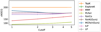
(a) MQ2008 dataset

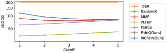
(b) Istella-S dataset

Figure 2. cNDCG of different prefix in the post-processing setting. FairK and MCFair overlap with each other, PLFair and ExploreK overlap.

In this section, we first compare fair methods’ fairness capacity, i.e., the maximum fairness a method can reach. Then we will discuss the effectiveness performance given different degree of fairness requirement.

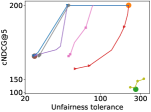
(a) MQ2008 (post-processing).

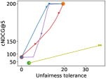
(b) Istella-S (post-processing).

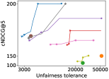
(c) MQ2008 (online).

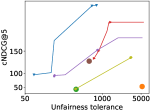
(d) Istella-S (online).

Figure 3. Effectiveness vs. unfairness tolerance in the post-processing setting (a,b) and the online setting (c,d). Given the same unfairness, the higher curves or points lie, the better their performances are.

5.2.1. Can MCFair reach fairness in the post-processing setting?

In Table 2, we compare different methods’ capacity to reach fairness, where we prioritize fairness by setting $\alpha$, if available, as the its maximum value. As shown in Table 2, fair ranking algorithms FairCo, LP, MCFair and FairK can significantly outperform unfair ranking algorithms in term of unfairness mitigation. The success of MCFair and FairK validates our assumption that fairness’s gradient can be directly used as ranking scores to optimize fairness. Besides, ILP and MMF show a slightly inferior fairness capacity and PLFair can not mitigate unfairness. More detail discussion and possible reason for their poor performance is in the next section.

Aside from unfairness, we also show the cNDCG performance of different prefixes in Figure 2 where $\alpha$ is set to the maximum for each method. In Table 2, unfair ranking method TopK can get the highest cNDCG performance as TopK only cares about effectiveness and sacrifices fairness. ExploreK only explores items and thus does not optimize fairness or effectiveness. All the fair algorithms except MMF and PLFair have very similar cNDCG@5 on both datasets which empirically shows that cNDCG@$k_{s}$ (here $k_{s}=5$) is fixed as we derived in Eq. 21. Although we use $\gamma=1$ for derivation in Eq. 21 while using $\gamma=0.995$ to calculate cNDCG@$k_{s}$, similar cNDCG@$k_{s}$ still holds. Despite similar cNDCG@5 and fairness, MCFair and FairK still significantly outperform other fair algorithms at the top ranks’ effectiveness. And we believe higher performance at top ranks’ is more important as users usually pay more attention (i.e., higher examining probability) to them.

Besides fairness capacity and effectiveness, we also empirically compare the time efficiency. In Table 2, ILP and LP are really time-consuming, while PLFair and MMF also need more time than other algorithms. While the other algorithms have similar time costs.

5.2.2. Can MCFair reach a better balance between fairness and effectiveness?

In the previous sections, we compare algorithms when they only care about fairness. However, such a comparison is not sufficient since different ranking systems may have different fairness and effectiveness requirements. To give a comprehensive comparison of different ranking methods, we compare ranking methods’ effectiveness-fairness balance given different fairness requirements.

In Figure 3(a) and Figure 3(b), we show the balance between fairness and effectiveness in the post-processing setting. To generate the balance curves, we incrementally sample $\alpha$ from the minimum value to the maximum value within $\alpha$’s ranges indicated in Section 5.1.2. After sampling, we carry out five independent experiments for each $\alpha$ to get the effectiveness and fairness pair based on the average performance of the five independent experiments. Then we connect different $\alpha$’s effectiveness-fairness pair to form a curve in Figure 3. The curves start from the right to the left as $\alpha$ increases, and we care more about fairness. Since TopK, ExploreK and FairK don’t have trade-off parameters, each one of them only have one single pair of effectiveness and fairness and their performances are shown as single points in Figure 3. Besides, the left bottom part of curves means caring fairness only, which corresponds to the results in Table 2 and Figure 2. All curves show a tradeoff between effectiveness and fairness, which means that mitigating more unfairness usually sacrifices effectiveness. The reason behind this tradeoff is that achieving fairness will bring constraints on optimizing effectiveness. Among all fair methods, our method MCFair significantly outperforms all other fair methods where MCFair reaches the best cNDCG given the same unfairness, i.e., MCFair’s curve lies higher. ILP, MMF, and PLFair can also show the tradeoff between effectiveness and fairness, although they have poor fairness capacities (discussed in Sec 5.2.1). As for the possible reason, the integer linear programming method used by ILP may not be effective in optimizing fairness. MMF actually follows a slightly different definition of fairness which require fairness at any cutoff should be fair. As for PLFair, PLFair tries to learn the ranking score that optimizes fairness based on the feature representation (the original setting in (Oosterhuis, 2021)). However, the feature representation is originally designed for relevance which makes PLFair suboptimal.

5.3. Results in the Online Setting.

In the above sections, we analyze the results in the post-processing setting where relevance is assumed to be given or already well-estimated. In this section, we will analyze the results in a more practical setting, i.e., the online setting, where ranking optimization and relevance estimation are carried out at the same time.

Figure 4. FairCo boosted by exploration with marginal certainty based exploration. (MQ2008)

Figure 5. Ablation study of MCFair with different combinations of the three parts in Eq. 23 on MQ2008. Only considering one part is shown as scatter point. When considering more than one part, we will get a curve which is generated by increasing weight of the last part. Arrow shows how curves develop when increasing the weight of the last part. For example, for Eff.+Uncert.+Fair. and Eff.+Fair., we increase the weights of Fair. i.e., fairness part, when optimizing a ranked list. With each different weight, we can get a (cNDCG@5, unfairness) pair when finishing experiments. And we connect pairs from different weights to form a curve. For Eff.+Uncert. and Fair.+Uncert., we increase the weights of uncertainty.

5.3.1. Can MCFair work in the online setting?

To study this problem, we show the balance between effectiveness and fairness of the online setting in Fig. 3(c) and Fig.  3(d). Similar to the post-processing setting, our method MCFair still outperforms all other baselines in the online setting. Since most of the results are similar to the post-processing setting in §5.2.2, we only discuss the difference. In Fig. 3(c) and Fig.  3(d), TopK cannot reach the highest effectiveness and FairK also can not reach the lowest unfairness in the online setting, which is different from the post-processing setting. We think the reason for the difference is that they naively trust the uncertain relevance estimation, which makes effectiveness optimization and fairness optimization fail (more discussion in §5.3.3).

5.3.2. Can marginal certainty help boost existing fair methods’ performance?

In this section, we investigate whether the marginal certainty-based exploration can boost existing fair methods. We mainly focus on how to boost FairCo and leave how to boost other fair methods for future study. Specifically, we directly add $\savestack{\tmpbox}{\stretchto{\scaleto{\scalerel*[width("MC")]{\kern-0.6pt\bigwedge\kern-0.6pt}{\rule[-505.89pt]{4.30554pt}{505.89pt}}}{}}{0.5ex}}\stackon[1pt]{MC}{\tmpbox}(d)$ (see Eq. 29), the marginal certainty, to FairCo’s ranking score, referred to as FairCo w/ Explor. As shown in Figure 4, FairCo w/ Explor. outperforms FairCo as it reaches better cNDCG given the same unfairness. FairCo w/ Explor.’s better performance shows marginal certainty can effectively boost FairCo. Our method MCFair still significantly outperforms FairCo w/ Explor.

5.3.3. Ablation study.

In this section, we conduct an ablation study to evaluate the significance of each part of MCFair. Since the ranking score of MCFair $\savestack{\tmpbox}{\stretchto{\scaleto{\scalerel*[width("ug")]{\kern-0.6pt\bigwedge\kern-0.6pt}{\rule[-505.89pt]{4.30554pt}{505.89pt}}}{}}{0.5ex}}\stackon[1pt]{ug}{\tmpbox}(d)$ in Eq. 24 has three parts, corresponding to effectiveness, fairness, and uncertainty respectively, there are a total of seven (${3\choose 1}+{3\choose 2}+{3\choose 3}=7$) combinations that need to be evaluated. The ablation results of each combination are shown in Figure 5. For the ablation results, considering more than two parts are shown as balance curves while considering only one part is shown as single points. In Figure 5, there is a very interesting cycle formed by the curves. In the cycle, considering all three parts, i.e., Eff.+Fair.+Uncer., outperform all other combinations since Eff.+Fair.+Uncer. can reach better effectiveness given the same unfairness.

6. Conclusions

In this work, we study the critical problem of relevance-fairness balance in online ranking settings. We propose a novel Marginal-Certainty-aware Fair Ranking algorithm named MCFair. MCFair jointly optimizes fairness and user utility while relevance estimation is constantly updated in an online manner. With extensive experiments on semi-synthesized datasets, MCFair shows its superior performance compared to other fair ranking algorithms.

References

- (1)
- Agarwal et al. (2019) Aman Agarwal, Ivan Zaitsev, Xuanhui Wang, Cheng Li, Marc Najork, and Thorsten Joachims. 2019. Estimating position bias without intrusive interventions. In Proceedings of the Twelfth ACM International Conference on Web Search and Data Mining. 474–482.
- Ai et al. (2018a) Qingyao Ai, Keping Bi, Jiafeng Guo, and W Bruce Croft. 2018a. Learning a deep listwise context model for ranking refinement. In The 41st international ACM SIGIR conference on research & development in information retrieval. 135–144.
- Ai et al. (2018b) Qingyao Ai, Keping Bi, Cheng Luo, Jiafeng Guo, and W Bruce Croft. 2018b. Unbiased learning to rank with unbiased propensity estimation. In SIGIR.
- Ai et al. (2021) Qingyao Ai, Tao Yang, Huazheng Wang, and Jiaxin Mao. 2021. Unbiased learning to rank: online or offline? TOIS (2021).
- Biega et al. (2018) Asia J Biega, Krishna P Gummadi, and Gerhard Weikum. 2018. Equity of attention: Amortizing individual fairness in rankings. In The 41st international acm sigir conference on research & development in information retrieval. 405–414.
- Chuklin et al. (2015) Aleksandr Chuklin, Ilya Markov, and Maarten de Rijke. 2015. Click models for web search. Synthesis lectures on information concepts, retrieval, and services 7, 3 (2015), 1–115.
- Cohen et al. (2021) Daniel Cohen, Bhaskar Mitra, Oleg Lesota, Navid Rekabsaz, and Carsten Eickhoff. 2021. Not All Relevance Scores are Equal: Efficient Uncertainty and Calibration Modeling for Deep Retrieval Models. In Proceedings of the 44th International ACM SIGIR Conference on Research and Development in Information Retrieval. 654–664.
- Craswell et al. (2008) Nick Craswell, Onno Zoeter, Michael Taylor, and Bill Ramsey. 2008. An experimental comparison of click position-bias models. In Proceedings of the 2008 international conference on web search and data mining. 87–94.
- Culpepper et al. (2016) J Shane Culpepper, Charles LA Clarke, and Jimmy Lin. 2016. Dynamic cutoff prediction in multi-stage retrieval systems. In Proceedings of the 21st Australasian Document Computing Symposium. 17–24.
- Draper (1995) David Draper. 1995. Assessment and propagation of model uncertainty. Journal of the Royal Statistical Society: Series B (Methodological) 57, 1 (1995), 45–70.
- Gal and Ghahramani (2016) Yarin Gal and Zoubin Ghahramani. 2016. Dropout as a bayesian approximation: Representing model uncertainty in deep learning. In international conference on machine learning. PMLR, 1050–1059.
- Hardy et al. (1952) Godfrey Harold Hardy, John Edensor Littlewood, George Pólya, György Pólya, et al. 1952. Inequalities. Cambridge university press.
- Hofmann et al. (2013) Katja Hofmann, Shimon Whiteson, and Maarten de Rijke. 2013. Balancing exploration and exploitation in listwise and pairwise online learning to rank for information retrieval. Information Retrieval 16, 1 (2013), 63–90.
- Järvelin and Kekäläinen (2002) Kalervo Järvelin and Jaana Kekäläinen. 2002. Cumulated gain-based evaluation of IR techniques. ACM Transactions on Information Systems (TOIS) (2002).
- Joachims et al. (2017) Thorsten Joachims, Laura Granka, Bing Pan, Helene Hembrooke, and Geri Gay. 2017. Accurately interpreting clickthrough data as implicit feedback. In ACM SIGIR Forum, Vol. 51. Acm New York, NY, USA, 4–11.
- Lien et al. (2019) Yen-Chieh Lien, Daniel Cohen, and W Bruce Croft. 2019. An assumption-free approach to the dynamic truncation of ranked lists. In Proceedings of the 2019 ACM SIGIR International Conference on Theory of Information Retrieval. 79–82.
- Liu et al. (2009) Tie-Yan Liu et al. 2009. Learning to rank for information retrieval. Foundations and Trends® in Information Retrieval 3, 3 (2009), 225–331.
- Lucchese et al. (2016) Claudio Lucchese, Franco Maria Nardini, Salvatore Orlando, Raffaele Perego, Fabrizio Silvestri, and Salvatore Trani. 2016. Post-learning optimization of tree ensembles for efficient ranking. In Proceedings of the 39th International ACM SIGIR conference on Research and Development in Information Retrieval. 949–952.
- Luo et al. (2022) Dan Luo, Lixin Zou, Qingyao Ai, Zhiyu Chen, Dawei Yin, and Brian D Davison. 2022. Model-based Unbiased Learning to Rank. arXiv preprint arXiv:2207.11785 (2022).
- Mehrabi et al. (2021) Ninareh Mehrabi, Fred Morstatter, Nripsuta Saxena, Kristina Lerman, and Aram Galstyan. 2021. A survey on bias and fairness in machine learning. ACM Computing Surveys (CSUR) 54, 6 (2021), 1–35.
- Morik et al. (2020) Marco Morik, Ashudeep Singh, Jessica Hong, and Thorsten Joachims. 2020. Controlling Fairness and Bias in Dynamic Learning-to-Rank. In Proceedings of the 43rd International ACM SIGIR Conference on Research and Development in Information Retrieval.
- Oosterhuis (2021) Harrie Oosterhuis. 2021. Computationally Efficient Optimization of Plackett-Luce Ranking Models for Relevance and Fairness. In SIGIR.
- Oosterhuis and de Rijke (2020) Harrie Oosterhuis and Maarten de Rijke. 2020. Policy-aware unbiased learning to rank for top-k rankings. In Proceedings of the 43rd International ACM SIGIR Conference on Research and Development in Information Retrieval. 489–498.
- Oosterhuis and de Rijke (2021) Harrie Oosterhuis and Maarten de Rijke. 2021. Unifying online and counterfactual learning to rank: A novel counterfactual estimator that effectively utilizes online interventions. In Proceedings of the 14th ACM International Conference on Web Search and Data Mining. 463–471.
- Penha and Hauff (2021) Gustavo Penha and Claudia Hauff. 2021. On the calibration and uncertainty of neural learning to rank models for conversational search. In Proceedings of the 16th Conference of the European Chapter of the Association for Computational Linguistics: Main Volume. 160–170.
- Qin and Liu (2013) Tao Qin and Tie-Yan Liu. 2013. Introducing LETOR 4.0 datasets. arXiv preprint arXiv:1306.2597 (2013).
- Radlinski and Joachims (2006) Filip Radlinski and Thorsten Joachims. 2006. Minimally invasive randomization for collecting unbiased preferences from clickthrough logs. In Proceedings of the national conference on artificial intelligence, Vol. 21. Menlo Park, CA; Cambridge, MA; London; AAAI Press; MIT Press; 1999, 1406.
- Roitman et al. (2017) Haggai Roitman, Shai Erera, and Bar Weiner. 2017. Robust standard deviation estimation for query performance prediction. In Proceedings of the ACM SIGIR International Conference on Theory of Information Retrieval. 245–248.
- Schuth et al. (2015) Anne Schuth, Robert-Jan Bruintjes, Fritjof Buüttner, Joost van Doorn, Carla Groenland, Harrie Oosterhuis, Cong-Nguyen Tran, Bas Veeling, Jos van der Velde, Roger Wechsler, et al. 2015. Probabilistic multileave for online retrieval evaluation. In Proceedings of the 38th international ACM SIGIR Conference on Research and Development in Information Retrieval. 955–958.
- Schuth et al. (2013) Anne Schuth, Katja Hofmann, Shimon Whiteson, and Maarten De Rijke. 2013. Lerot: An online learning to rank framework. In Proceedings of the 2013 workshop on Living labs for information retrieval evaluation. 23–26.
- Schuth et al. (2016) Anne Schuth, Harrie Oosterhuis, Shimon Whiteson, and Maarten de Rijke. 2016. Multileave gradient descent for fast online learning to rank. In Proceedings of the Ninth ACM International Conference on Web Search and Data Mining. 457–466.
- Singh and Joachims (2018) Ashudeep Singh and Thorsten Joachims. 2018. Fairness of exposure in rankings. In Proceedings of the 24th ACM SIGKDD International Conference on Knowledge Discovery & Data Mining. 2219–2228.
- Singh and Joachims (2019) Ashudeep Singh and Thorsten Joachims. 2019. Policy learning for fairness in ranking. Advances in Neural Information Processing Systems 32 (2019).
- Singh et al. (2021) Ashudeep Singh, David Kempe, and Thorsten Joachims. 2021. Fairness in ranking under uncertainty. Advances in Neural Information Processing Systems 34 (2021).
- Smucker et al. (2007) Mark D Smucker, James Allan, and Ben Carterette. 2007. A comparison of statistical significance tests for information retrieval evaluation. In Proceedings of the sixteenth ACM conference on Conference on information and knowledge management. 623–632.
- Tran et al. (2021) Anh Tran, Tao Yang, and Qingyao Ai. 2021. ULTRA: An Unbiased Learning To Rank Algorithm Toolbox. In Proceedings of the 30th ACM International Conference on Information & Knowledge Management. 4613–4622.
- Tran et al. (2022) Anh Tran, Tao Yang, and Qingyao Ai. 2022. UTIRL at the NTCIR-16 ULTRE Task. (2022).
- Wang et al. (2019) Huazheng Wang, Sonwoo Kim, Eric McCord-Snook, Qingyun Wu, and Hongning Wang. 2019. Variance reduction in gradient exploration for online learning to rank. In Proceedings of the 42nd International ACM SIGIR Conference on Research and Development in Information Retrieval. 835–844.
- Wang et al. (2018) Xuanhui Wang, Nadav Golbandi, Michael Bendersky, Donald Metzler, and Marc Najork. 2018. Position bias estimation for unbiased learning to rank in personal search. In Proceedings of the Eleventh ACM International Conference on Web Search and Data Mining. 610–618.
- Wu et al. (2021) Yao Wu, Jian Cao, Guandong Xu, and Yudong Tan. 2021. Tfrom: A two-sided fairness-aware recommendation model for both customers and providers. In Proceedings of the 44th International ACM SIGIR Conference on Research and Development in Information Retrieval. 1013–1022.
- Xu et al. (2022) Zhichao Xu, Anh Tran, Tao Yang, and Qingyao Ai. 2022. Reinforcement Learning to Rank with Coarse-grained Labels. arXiv preprint arXiv:2208.07563 (2022).
- Yang and Ai (2021) Tao Yang and Qingyao Ai. 2021. Maximizing Marginal Fairness for Dynamic Learning to Rank. In Proceedings of the Web Conference 2021. 137–145.
- Yang et al. (2020) Tao Yang, Shikai Fang, Shibo Li, Yulan Wang, and Qingyao Ai. 2020. Analysis of multivariate scoring functions for automatic unbiased learning to rank. In Proceedings of the 29th ACM International Conference on Information & Knowledge Management. 2277–2280.
- Yang et al. (2022a) Tao Yang, Chen Luo, Hanqing Lu, Parth Gupta, Bing Yin, and Qingyao Ai. 2022a. Can Clicks Be Both Labels and Features? Unbiased Behavior Feature Collection and Uncertainty-Aware Learning to Rank. In Proceedings of the 45th International ACM SIGIR Conference on Research and Development in Information Retrieval.
- Yang et al. (2022b) Tao Yang, Zhichao Xu, and Qingyao Ai. 2022b. Effective Exposure Amortizing for Fair Top-k Recommendation. arXiv preprint arXiv:2204.03046 (2022).
- Yue and Joachims (2009) Yisong Yue and Thorsten Joachims. 2009. Interactively optimizing information retrieval systems as a dueling bandits problem. In Proceedings of the 26th Annual International Conference on Machine Learning. 1201–1208.
- Zehlike et al. (2017) Meike Zehlike, Francesco Bonchi, Carlos Castillo, Sara Hajian, Mohamed Megahed, and Ricardo Baeza-Yates. 2017. Fa* ir: A fair top-k ranking algorithm. In Proceedings of the 2017 ACM on Conference on Information and Knowledge Management. 1569–1578.
- Zehlike and Castillo (2020) Meike Zehlike and Carlos Castillo. 2020. Reducing disparate exposure in ranking: A learning to rank approach. In Proceedings of The Web Conference 2020.
- Zehlike et al. (2022) Meike Zehlike, Tom Sühr, Ricardo Baeza-Yates, Francesco Bonchi, Carlos Castillo, and Sara Hajian. 2022. Fair Top-k Ranking with multiple protected groups. Information Processing & Management 59, 1 (2022), 102707.
- Zhao et al. (2022) Yurou Zhao, Zechun Niu, Feng Wang, Jiaxin Mao, Qingyao Ai, Tao Yang, Junqi Zhang, and Yiqun Liu. 2022. Overview of the NTCIR-16 Unbiased Learning to Rank Evaluation (ULTRE) Task. In Proceedings of the NTCIR-16 Conference on Evaluation of Information Access Technologies.
- Zhu et al. (2009) Jianhan Zhu, Jun Wang, Michael Taylor, and Ingemar J Cox. 2009. Risk-aware information retrieval. In European Conference on Information Retrieval. Springer.