AdaTranS: Adapting with Boundary-based Shrinking for End-to-End
Speech Translation

Abstract

To alleviate the data scarcity problem in End-to-end speech translation (ST), pre-training on data for speech recognition and machine translation is considered as an important technique. However, the modality gap between speech and text prevents the ST model from efficiently inheriting knowledge from the pre-trained models. In this work, we propose AdaTranS for end-to-end ST. It adapts the speech features with a new shrinking mechanism to mitigate the length mismatch between speech and text features by predicting word boundaries. Experiments on the MUST-C dataset demonstrate that AdaTranS achieves better performance than the other shrinking-based methods, with higher inference speed and lower memory usage. Further experiments also show that AdaTranS can be equipped with additional alignment losses to further improve performance.

1 Introduction

End-to-end speech translation (ST), which directly translates source speech into text in another language, has achieved remarkable progress in recent years Duong et al. (2016); Weiss et al. (2017); Berard et al. (2018); Wang et al. (2020); Xu et al. (2021); Ye et al. (2022). Compared to the conventional cascaded systems Ney (1999); Mathias and Byrne (2006), the end-to-end models are believed to have the advantages of low latency and less error propagation. A well-trained end-to-end model typically needs a large amount of training data. However, the available direct speech-translation corpora are very limited Di Gangi et al. (2019). Given the fact that data used for automatic speech recognition (ASR) and machine translation (MT) are much richer, the paradigm of “pre-training on ASR and MT data and then fine-tuning on ST” becomes one of the approaches to alleviate the data scarcity problem Bansal et al. (2019); Xu et al. (2021).

It has been shown that decoupling the ST encoder into acoustic and semantic encoders is beneficial to learn desired features Liu et al. (2020); Zeng et al. (2021). Initializing the two encoders by pre-trained ASR and MT encoders, respectively, can significantly boost the performance Xu et al. (2021). However, the modality gap between speech and text might prevent the ST models from effectively inheriting the pre-trained knowledge Xu et al. (2021).

The modality gap between speech and text can be summarized as two dimensions. First, the length gap – the speech features are usually much longer than their corresponding texts Chorowski et al. (2015); Liu et al. (2020). Second is the representation space gap. Directly fine-tuning MT parameters (semantic encoder and decoder) with speech features as inputs, which learned independently, would result in sub-optimal performance. Previous work has explored and proposed several alignment objectives to address the second gap, e.g., Cross-modal Adaption Liu et al. (2020), Cross-Attentive Regularization Tang et al. (2021a) and Cross-modal Contrastive Ye et al. (2022).

A shrinking mechanism is usually used to address the length gap. Some leverage Continuous Integrate-and-Fire (CIF) Dong and Xu (2020) to shrink the long speech features Dong et al. (2022); Chang and Lee (2022), but they mostly work on simultaneous ST and need extra efforts to perform better shrinking. Others mainly depend on the CTC greedy path Liu et al. (2020); Gaido et al. (2021), which might introduce extra inference cost and lead to sub-optimal shrinking results. AdaTranS uses a new shrinking mechanism called boundary-based shrinking, which achieves higher performance.

Through extensive experiments on the MUST-C Di Gangi et al. (2019) dataset, we show that AdaTranS is superior to other shrinking-based methods with a faster inference speed or lower memory usage. Further equipped with alignment objectives, AdaTranS shows competitive performance compared to the state-of-the-art models.

2 Proposed Model: AdaTranS

2.1 Architecture

Following previous studies Liu et al. (2020); Xu et al. (2021), AdaTranS decouples the ST encoder into an acoustic encoder and a semantic encoder. To bridge the modality gap between speech and text, an adaptor is usually needed before the semantic encoder. We choose the shrinking operation Liu et al. (2020); Zeng et al. (2021) as our adaptor, where the long speech sequences are shrunk to the similar lengths as the transcription based on designed mechanisms (details will be introduced in the next subsection). The shrunk representations are sent to the semantic encoder to derive the encoder output. Finally, the semantic output is fed into the ST decoder for computing the cross-entropy loss:

$$\mathcal{L}_{ST}=-\sum_{|\mathcal{D}_{ST}|}\,\sum_{t=1}^{T_{y}}\text{log}\,p(y_{t}|y_{<t},\bm{x})$$ (1)

To incorporate extra ASR and MT data, we use the pre-trained ASR encoder to initialize the ST acoustic encoder, and the pre-trained MT encoder and decoder to initialize the ST semantic encoder and decoder, respectively. Both pre-trained models are first trained with extra ASR (or MT) data and then fine-tuned with the in-domain data (the ASR part or MT part in the ST corpus). Figure 1 displays our architecture as well as the training process.

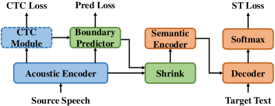
Figure 1: AdaTranS Architecture, where the blue modules are initialized with the ASR model and the orange modules are initialized with the MT model. The CTC module (dotted) can be removed during inference.

2.2 Boundary-based Shrinking Mechanism

Previous shrinking mechanisms Liu et al. (2020); Zeng et al. (2021) mostly depend on a CTC module Graves et al. (2006) to produce token-label probabilities for each frame in the speech representations. Then, a word boundary is recognized if the labeled tokens of two consecutive frames are different. There are two main drawbacks to such CTC-based methods. First, the word boundaries are indirectly estimated and potentially affected by error propagation from the token label predictions which are usually greedily estimated by the argmax operation on the CTC output probabilities. Second, the token labels are from a large source vocabulary resulting in extra parameters and computation cost in the CTC module during inference.

We introduce a boundary-based shrinking mechanism to address the two drawbacks. A boundary predictor is used to directly predict the probability of each speech representation being a boundary, which is then used for weighted shrinking. Since the boundary labels on the speech representations are unknown during training, we introduce signals from the CTC module to guide the training of the boundary predictor. The CTC module will be discarded during inference. Below shows the details.

CTC module.

We first briefly introduce the CTC module. It predicts a path $\bm{\pi}=(\pi_{1},\pi_{2},...,\pi_{T_{x}})$, where $T_{x}$ is the length of hidden states after the acoustic encoder. And $\pi_{t}\in\mathcal{V}\cup\{\phi\}$ can be either a token in the source vocabulary $\mathcal{V}$ or the blank symbol $\phi$. By removing blank symbols and consecutively repeated labels, denoted as an operation $\mathcal{B}$, we can map the CTC path to the corresponding transcription. A CTC loss is defined as the probability of all possible paths that can be mapped to the ground-truth transcription $\bm{z}$:

$$\mathcal{L}_{CTC}=-\sum_{|\mathcal{D}_{ST}|}\,\sum_{\bm{\pi}\in\mathcal{B}^{-1}(\bm{z})}\text{log}\,p(\bm{\pi}|\bm{H}^{A})$$ (2)

CTC-guided Boundary Predictor.

We propose to use a boundary predictor to replace the CTC module, which has a similar architecture but with only three labels. The three labels are <BK> (blank label), <BD> (boundary label) and <OT> (others), respectively. However, the ground-truth labels for training the predictor are unknown. Therefore, we introduce soft training signals based on the output probabilities of the CTC module. Specifically, the ground-truth probabilities of each frame $t$ to be labeled as the three labels are defined as:

$$\begin{split}&p^{\prime}_{t}(\text{<BK>})=p(\pi_{t}=\phi)\\ &p^{\prime}_{t}(\text{<BD>})=\sum\nolimits_{i\neq\phi}p(\pi_{t}=i)p(\pi_{t+1}\neq i)\\ &p^{\prime}_{t}(\text{<OT>})=1-p^{\prime}_{t}(\text{<BK>})-p^{\prime}_{t}(\text{<BD>})\\ \end{split}$$ (3)

Then, the objective for the boundary predictor is:

$$\mathcal{L}_{Pred}=-\sum_{|\mathcal{D}_{ST}|}\sum_{t=1}^{T^{\prime}_{x}}\sum_{i\in\Delta}p^{\prime}_{t}(i)\;\text{log}\,p_{t}(i)$$ (4)

where $\Delta=\{\text{<BK>},\text{<BD>},\text{<OT>}\}$. The CTC module is only used in the training process and can be discarded during inference. Since the number of labels in the predictor is significantly smaller than the size of the source vocabulary, the time and computation costs introduced by the predictor are negligible. Figure 2 shows an example to elaborate the advantage of such a predictor.

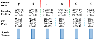
Figure 2: An example of CTC probabilities (we assume there are three tokens in vocabulary for simplification), together with the corresponding boundary predictor soft signals and ground labels. We will get different boundary detection results based on their label probabilities (the solid and dotted lines). CTC argmax path predicts the wrong boundaries and we can get correct boundaries if we set the threshold $\theta$ as 0.5 in boundary predictor.

Weighted Shrinking.

For shrinking, we define boundary frames as those with the probabilities of the <BD> label higher than a pre-defined threshold $\theta$. The frames between two boundary frames are defined as one segment, which can be aligned to one source token. Inspired by Zeng et al. (2021), we sum over the frames in one segment weighted by their probabilities of being blank labels to distinguish informative and non-informative frames:

$$\bm{h}^{A}_{t^{\prime}}=\sum_{t\in seg\,t^{\prime}}\bm{h}^{A}_{t}\frac{\exp(\mu(1-p_{t}(\text{<BK>})))}{\sum_{s\in seg\,t^{\prime}}\exp(\mu(1-p_{s}(\text{<BK>})))}$$ (5)

where $\mu\geq 0$ denotes the temperature for the Softmax Function.

Forced Training.

We introduce a forced training trick to explicitly solve the length mismatch between speech and text representations. During training, we set the threshold $\theta$ dynamically based on the length of $\bm{z}$ to make sure the shrunk representations have exactly the same lengths as their corresponding transcriptions. Specifically, we first sort the probabilities to be <BD> of all frames in descending order, and then select the $T_{z}$-th one as the threshold $\theta$.

2.3 Training Objectives

The total loss of our AdaTranS will be:

$$\mathcal{L}=\mathcal{L}_{ST}+\alpha\cdot\mathcal{L}_{CTC}+\beta\cdot\mathcal{L}_{Pred}$$ (6)

where $\alpha$, $\beta$ are hyper parameters that control the effects of different losses.

3 Experiments

3.1 Experimental Setup

Datasets.

We conduct experiments on three language pairs of MUST-C dataset Di Gangi et al. (2019): English-German (En–De), English-French (En–Fr) and English-Russian (En–Ru). We use the official data splits for train and development and tst-COMMON for test. We use LibriSpeech Panayotov et al. (2015) as the extra ASR data to pre-train the acoustic model. OpenSubtitles2018 or WMT14 are used to pre-train the MT model. The data statistics are listed in Table 3 of Appendix A.

Preprocessing.

We use 80D log-mel filterbanks as speech input features and SentencePiece Kudo and Richardson (2018) to generate subword vocabularies for each language pair. Each vocabulary is learned on all the texts from ST and MT data and shared across source and target languages, with a total size of 16000. More details please refer to the Appendix B.

Model Setting.

Conv-Transformer Huang et al. (2020) or Conformer Gulati et al. (2020) (results in Table 2 are achieved by AdaTranS with Conformer) is used as our acoustic encoder, both containing 12 layers. For the semantic encoder and ST decoder, we follow the general NMT Transformer settings (i.e., both contain 6 layers). Each Transformer layer has an input embedding dimension of 512 and a feed-forward layer dimension of 2048. The hyper-parameters in Eq. 6 are set as: $\alpha=1.0$ and $\beta=1.0$, respectively. The temperature of the softmax function in Eq. 5 ($\mu$) is $1.0$, while the threshold $\theta$ in the boundary predictor is set to $0.4$ during inference. All the above hyper-parameters are set through grid search based on the performance of the development set. Training details please refer to Appendix B.

We apply SacreBLEU for evaluation, where case-sensitive detokenized BLEU is reported.

3.2 Experiment results

Model	Diff$\leq$2	Speedup	Mem	BLEU
	(%)		Usage	En-De	En-Fr
No Shrink	–	1.00$\times$	1.00	26.0	36.8
Fix Shrink	36.7	1.06$\times$	0.74	25.4	36.0
CIF-Based	70.3	1.04$\times$	0.74	25.8	36.2
CTC-Based	80.2	0.76$\times$	1.77	26.4	36.9
Boundary-Based	81.9	1.06$\times$	0.78	26.7	37.4
- Forced Train				26.4	37.1
- Blank Label				26.3	36.6

Table 1: The results of shrinking-based methods and the corresponding shrinking quality, evaluated with length differences between the shrunk representations and transcriptions. Diff$\leq$2 means the length differences are less than or equal to 2. The speedup and memory usage are both tested with a batch size of 16, and we only display the relative values for clear comparison.

Table 1 compares different shrinking-based methods in terms of quality and efficiency. Besides translation quality, we use length differences between the shrunk representations and the corresponding transcriptions to evaluate shrinking quality following Zeng et al. (2021). We use inference speedup and memory usage to evaluate the efficiency.

For comparisons, the Fix-Shrink method shrinks the speech features with a fixed rate (e.g. every 3 frames). The CIF-Based method Dong et al. (2022) is based on a continuous integrate-and-fire mechanism. The CTC-Based method Liu et al. (2020) shrinks features based on CTC greedy paths. As can be seen, poor shrinking (Fix-Shrink and CIF-based) hurts the performance, although with better efficiency. The boundary-based shrinking used in AdaTranS and the CTC-based method achieve better shrinking quality, with performance improved. However, CTC-Based method hurts the inference efficiency (lower inference speed and higher memory usage) as they introduce extra computation cost producing greedy CTC path in a large source vocabulary. Our method performs the best in both shrinking and translation quality with nice inference efficiency. This demonstrates the effectiveness of our method.

On the other hand, we also notice that removing forced training trick (“-Forced Train”) or weighted-shrinking (i.e., “-Blank Label”, simply average the frame representations rather than use Eq. 5) will affects the translation quality, showing the effectiveness of these two components.

Adopting Alignment Objectives.

Model	BLEU
	En-De	En-Fr	En-Ru
MT	34.4	44.9	21.3
Cascaded Model	28.1	37.0	17.6
STPT† Tang et al. (2022)	29.2	39.7	–
SpeechUT† Zhang et al. (2022)	30.1	41.4	–
JT-S-MT Tang et al. (2021a)	26.8	37.4	–
Chimera Han et al. (2021)	27.1	35.6	17.4
XSTNet Ye et al. (2021)	27.1	38.0	18.5
SATE Xu et al. (2021)	28.1	–	–
STEMM Fang et al. (2022)	28.7	37.4	17.8
ConST Ye et al. (2022)	28.3	38.3	18.9
AdaTranS	28.7	38.7	19.0

Table 2: Comparisons with the SOTA models. The first two rows are results with our pre-trained MT model and ASR model. Models marked with ^† are trained with complex speech-text joint pre-training techniques.

AdaTranS can be further improved with objectives that aligning speech and text representations (i.e. bridging the representation space gap introduced in Section 1). Table 2 shows the results of AdaTranS equipped with Cross-model Contrastive Ye et al. (2022) and knowledge distillation guided by MT. The results show that AdaTranS achieves competitive results in all the three datasets compared to previous state-of-the-art models.

Influence of the Boundary Threshold.

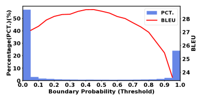
Figure 3: The distribution of probabilities for boundary prediction, and the corresponding model performance (BLEU) when using different values as threshold.

We also examine the effects of the threshold $\theta$ for the boundary predictor. Figure 3 shows the distribution of the predicted boundary probability (i.e. $p_{t}(\text{<BD>})$) for each frame in the MUST-C En–De test set. We find that the boundary predictor is confident ($<0.1$ and $>0.9$) in most cases. However, even though only a small portion of predictions are in the range of $[0.1,0.9]$, they significantly affect the BLEU scores when the threshold changes (the red line in Figure 3). The model achieves the best performance when the threshold is around $0.4$.

4 Conclusion

This work proposes a new end-to-end ST model called AdaTranS, which uses a boundary predictor trained by signals from CTC output probabilities, to adapt and bridge the length gap between speech and text. Experiments show that AdaTranS performs better than other shrinking-based methods, in terms of both quality and efficiency. It can also be further enhanced by modality alignment objectives to achieve state-of-the-art results.

Appendix A Data Statistics.

Table 3 shows the data statistics of the used datasets. ST datasets are all from MUST-C, and LibriSpeech serves as extra ASR data. MT data either comes from OpenSubtitles2018 or WMT14 following previous work settings.

Corpus	ST(Hours/#Sents)	ASR(Hours)	MT(#Sents)
En–De	408/234K	960	18M(OS)
En–Fr	492/280K	960	18M(WMT)
En–Ru	489/270K	960	2.5M(WMT)

Table 3: The statistics for the three language pairs. OS: OpenSubtiles2018. WMT: WMT14.

Appendix B Implementation Details.

Data Preprocessing.

We use 80D log-mel filterbanks as speech input features, which are calculated with 25ms window size and 10ms step size and normalized by utterance-level Cepstral Mean and Variance Normalization (CMVN). All the texts in ST and MT data are preprocessed in the same way, which are case-sensitive with punctuation preserved. We filter out samples with more than 3000 frames, over 256 tokens, or whose ratios of source and target text lengths are outside the range [2/3, 3/2]. We use SentencePiece Kudo and Richardson (2018) to generate subword vocabularies for each language pair. Each vocabulary is learned on all the texts from ST and MT data and shared across source and target languages, with a total size of 16000.

Training Details.

We train all the models using Adam optimizer Kingma and Ba (2015) with a 0.002 learning rate and 10000 warm-up steps followed by the inverse square root scheduler. Label smoothing and dropout strategies are used, both set to 0.1. The models are fine-tuned on 8 NVIDIA Tesla V100 GPUs with 40000 steps. The batch size is set to 40000 frames per GPU. We save checkpoints every epoch and average the last 10 checkpoints for evaluation with a beam size of 10.

Appendix C More Analysis.

Better Source-Target Alignment.

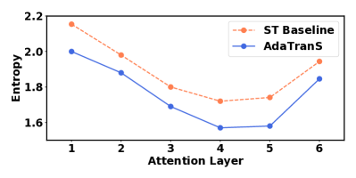
Figure 4: The attention entropy of each attention layer for end-to-end ST baseline and our model.

We evaluate the entropy of the cross attention from the ST baseline and AdaTranS. Let $\alpha_{ij}$ be the attention weight for a target token $y_{i}$ and a source speech feature (after shrinking) $x_{j}$, the entropy for each target token is defined as $E_{i}=-\sum\nolimits_{j=1}^{|x|}\alpha_{ij}\log\alpha_{ij}$. We then average the attention entropy of all target tokens in the test set. Lower entropy means the attention mechanism is more confident and concentrates on the source-target alignment. Figure 4 shows the entropy of different decoder layers. AdaTranS exhibits consistently lower entropy than the ST baseline. This means that our shrinking mechanism improves the learning of attention distributions.

Influence of Text Input Representations.

	SPM	SPM w/o Punct	Phoneme
MT
1. Only MUST-C Data	30.7	28.3	28.2
2. PT with Extra Data	34.4	31.6	29.5
ST
Initialized with Model 2	26.0	25.8	25.6

Table 4: BLEU scores of different text input representations in MUST-C En-De. SPM means using the subword units learned from a sentencepiece model, while “w/o Punct” indicates that punctuation is removed.

Representing text input with phonemes helps reduce the differences between speech and text Tang et al. (2021a, b). However, word representations and punctuation are important for learning semantic information, which are usually ignored when phonemes are used in prior works. Table 4 shows the MT results when using different text input representations, together with the ST performance that is initialized from the corresponding MT model. We can observe that the performance of downstream ST model is affected by the pre-trained MT model. Therefore, instead of following prior phoneme-level work for pre-training the MT, in this work we use subword units with punctuation and incorporate the shrinking mechanism to mitigate the length gap.

References

- Bansal et al. (2019) Sameer Bansal, Herman Kamper, Karen Livescu, Adam Lopez, and Sharon Goldwater. 2019. Pre-training on high-resource speech recognition improves low-resource speech-to-text translation. In Proceedings of the 2019 Conference of the North American Chapter of the Association for Computational Linguistics: Human Language Technologies, Volume 1 (Long and Short Papers), pages 58–68, Minneapolis, Minnesota. Association for Computational Linguistics.
- Berard et al. (2018) Alexandre Berard, Laurent Besacier, Ali Can Kocabiyikoglu, and Olivier Pietquin. 2018. End-to-end automatic speech translation of audiobooks. In 2018 IEEE International Conference on Acoustics, Speech and Signal Processing, ICASSP 2018, Calgary, AB, Canada, April 15-20, 2018, pages 6224–6228. IEEE.
- Chang and Lee (2022) Chih-Chiang Chang and Hung-yi Lee. 2022. Exploring continuous integrate-and-fire for adaptive simultaneous speech translation. In Interspeech 2022, 23rd Annual Conference of the International Speech Communication Association, Incheon, Korea, 18-22 September 2022, pages 5175–5179. ISCA.
- Chorowski et al. (2015) Jan Chorowski, Dzmitry Bahdanau, Dmitriy Serdyuk, Kyunghyun Cho, and Yoshua Bengio. 2015. Attention-based models for speech recognition. In Advances in Neural Information Processing Systems 28: Annual Conference on Neural Information Processing Systems 2015, December 7-12, 2015, Montreal, Quebec, Canada, pages 577–585.
- Di Gangi et al. (2019) Mattia A. Di Gangi, Roldano Cattoni, Luisa Bentivogli, Matteo Negri, and Marco Turchi. 2019. MuST-C: a Multilingual Speech Translation Corpus. In Proceedings of the 2019 Conference of the North American Chapter of the Association for Computational Linguistics: Human Language Technologies, Volume 1 (Long and Short Papers), pages 2012–2017, Minneapolis, Minnesota. Association for Computational Linguistics.
- Dong and Xu (2020) Linhao Dong and Bo Xu. 2020. CIF: continuous integrate-and-fire for end-to-end speech recognition. In 2020 IEEE International Conference on Acoustics, Speech and Signal Processing, ICASSP 2020, Barcelona, Spain, May 4-8, 2020, pages 6079–6083. IEEE.
- Dong et al. (2022) Qian Dong, Yaoming Zhu, Mingxuan Wang, and Lei Li. 2022. Learning when to translate for streaming speech. In Proceedings of the 60th Annual Meeting of the Association for Computational Linguistics (Volume 1: Long Papers), pages 680–694. Association for Computational Linguistics.
- Duong et al. (2016) Long Duong, Antonios Anastasopoulos, David Chiang, Steven Bird, and Trevor Cohn. 2016. An attentional model for speech translation without transcription. In Proceedings of the 2016 Conference of the North American Chapter of the Association for Computational Linguistics: Human Language Technologies, pages 949–959, San Diego, California. Association for Computational Linguistics.
- Fang et al. (2022) Qingkai Fang, Rong Ye, Lei Li, Yang Feng, and Mingxuan Wang. 2022. STEMM: Self-learning with speech-text manifold mixup for speech translation. In Proceedings of the 60th Annual Meeting of the Association for Computational Linguistics (Volume 1: Long Papers). Association for Computational Linguistics.
- Gaido et al. (2021) Marco Gaido, Mauro Cettolo, Matteo Negri, and Marco Turchi. 2021. CTC-based compression for direct speech translation. In Proceedings of the 16th Conference of the European Chapter of the Association for Computational Linguistics: Main Volume, pages 690–696, Online. Association for Computational Linguistics.
- Graves et al. (2006) Alex Graves, Santiago Fernández, Faustino J. Gomez, and Jürgen Schmidhuber. 2006. Connectionist temporal classification: labelling unsegmented sequence data with recurrent neural networks. In Machine Learning, Proceedings of the Twenty-Third International Conference (ICML 2006), Pittsburgh, Pennsylvania, USA, June 25-29, 2006, volume 148 of ACM International Conference Proceeding Series, pages 369–376. ACM.
- Gulati et al. (2020) Anmol Gulati, James Qin, Chung-Cheng Chiu, Niki Parmar, Yu Zhang, Jiahui Yu, Wei Han, Shibo Wang, Zhengdong Zhang, Yonghui Wu, and Ruoming Pang. 2020. Conformer: Convolution-augmented transformer for speech recognition. In Interspeech 2020, 21st Annual Conference of the International Speech Communication Association, Virtual Event, Shanghai, China, 25-29 October 2020, pages 5036–5040. ISCA.
- Han et al. (2021) Chi Han, Mingxuan Wang, Heng Ji, and Lei Li. 2021. Learning shared semantic space for speech-to-text translation. In Findings of the Association for Computational Linguistics: ACL-IJCNLP 2021, pages 2214–2225, Online. Association for Computational Linguistics.
- Huang et al. (2020) Wenyong Huang, Wenchao Hu, Yu Ting Yeung, and Xiao Chen. 2020. Conv-transformer transducer: Low latency, low frame rate, streamable end-to-end speech recognition. In Interspeech 2020, 21st Annual Conference of the International Speech Communication Association, Virtual Event, Shanghai, China, 25-29 October 2020, pages 5001–5005. ISCA.
- Kingma and Ba (2015) Diederik P. Kingma and Jimmy Ba. 2015. Adam: A method for stochastic optimization. In 3rd International Conference on Learning Representations, ICLR 2015, San Diego, CA, USA, May 7-9, 2015, Conference Track Proceedings.
- Kudo and Richardson (2018) Taku Kudo and John Richardson. 2018. SentencePiece: A simple and language independent subword tokenizer and detokenizer for neural text processing. In Proceedings of the 2018 Conference on Empirical Methods in Natural Language Processing: System Demonstrations, pages 66–71, Brussels, Belgium. Association for Computational Linguistics.
- Liu et al. (2020) Yuchen Liu, Junnan Zhu, Jiajun Zhang, and Chengqing Zong. 2020. Bridging the modality gap for speech-to-text translation. CoRR, abs/2010.14920.
- Mathias and Byrne (2006) Lambert Mathias and William Byrne. 2006. Statistical phrase-based speech translation. In 2006 IEEE International Conference on Acoustics Speech and Signal Processing, ICASSP 2006, Toulouse, France, May 14-19, 2006, pages 561–564. IEEE.
- Ney (1999) Hermann Ney. 1999. Speech translation: coupling of recognition and translation. In Proceedings of the 1999 IEEE International Conference on Acoustics, Speech, and Signal Processing, ICASSP ’99, Phoenix, Arizona, USA, March 15-19, 1999, pages 517–520. IEEE Computer Society.
- Panayotov et al. (2015) Vassil Panayotov, Guoguo Chen, Daniel Povey, and Sanjeev Khudanpur. 2015. Librispeech: An ASR corpus based on public domain audio books. In 2015 IEEE International Conference on Acoustics, Speech and Signal Processing, ICASSP 2015, South Brisbane, Queensland, Australia, April 19-24, 2015, pages 5206–5210. IEEE.
- Tang et al. (2022) Yun Tang, Hongyu Gong, Ning Dong, Changhan Wang, Wei-Ning Hsu, Jiatao Gu, Alexei Baevski, Xian Li, Abdelrahman Mohamed, Michael Auli, and Juan Pino. 2022. Unified speech-text pre-training for speech translation and recognition. In Proceedings of the 60th Annual Meeting of the Association for Computational Linguistics (Volume 1: Long Papers). Association for Computational Linguistics.
- Tang et al. (2021a) Yun Tang, Juan Pino, Xian Li, Changhan Wang, and Dmitriy Genzel. 2021a. Improving speech translation by understanding and learning from the auxiliary text translation task. In Proceedings of the 59th Annual Meeting of the Association for Computational Linguistics and the 11th International Joint Conference on Natural Language Processing (Volume 1: Long Papers), pages 4252–4261, Online. Association for Computational Linguistics.
- Tang et al. (2021b) Yun Tang, Juan Miguel Pino, Changhan Wang, Xutai Ma, and Dmitriy Genzel. 2021b. A general multi-task learning framework to leverage text data for speech to text tasks. In IEEE International Conference on Acoustics, Speech and Signal Processing, ICASSP 2021, Toronto, ON, Canada, June 6-11, 2021, pages 6209–6213. IEEE.
- Wang et al. (2020) Chengyi Wang, Yu Wu, Shujie Liu, Ming Zhou, and Zhenglu Yang. 2020. Curriculum pre-training for end-to-end speech translation. In Proceedings of the 58th Annual Meeting of the Association for Computational Linguistics, pages 3728–3738, Online. Association for Computational Linguistics.
- Weiss et al. (2017) Ron J. Weiss, Jan Chorowski, Navdeep Jaitly, Yonghui Wu, and Zhifeng Chen. 2017. Sequence-to-sequence models can directly transcribe foreign speech. CoRR, abs/1703.08581.
- Xu et al. (2021) Chen Xu, Bojie Hu, Yanyang Li, Yuhao Zhang, Shen Huang, Qi Ju, Tong Xiao, and Jingbo Zhu. 2021. Stacked acoustic-and-textual encoding: Integrating the pre-trained models into speech translation encoders. In Proceedings of the 59th Annual Meeting of the Association for Computational Linguistics and the 11th International Joint Conference on Natural Language Processing (Volume 1: Long Papers), pages 2619–2630, Online. Association for Computational Linguistics.
- Ye et al. (2021) Rong Ye, Mingxuan Wang, and Lei Li. 2021. End-to-end speech translation via cross-modal progressive training. In Interspeech 2021, 22nd Annual Conference of the International Speech Communication Association, Brno, Czechia, 30 August - 3 September 2021, pages 2267–2271. ISCA.
- Ye et al. (2022) Rong Ye, Mingxuan Wang, and Lei Li. 2022. Cross-modal contrastive learning for speech translation. In Proceedings of the 2022 Conference of the North American Chapter of the Association for Computational Linguistics: Human Language Technologies, pages 5099–5113. Association for Computational Linguistics.
- Zeng et al. (2021) Xingshan Zeng, Liangyou Li, and Qun Liu. 2021. RealTranS: End-to-end simultaneous speech translation with convolutional weighted-shrinking transformer. In Findings of the Association for Computational Linguistics: ACL-IJCNLP 2021, pages 2461–2474, Online. Association for Computational Linguistics.
- Zhang et al. (2022) Ziqiang Zhang, Long Zhou, Junyi Ao, Shujie Liu, Lirong Dai, Jinyu Li, and Furu Wei. 2022. Speechut: Bridging speech and text with hidden-unit for encoder-decoder based speech-text pre-training. In EMNLP2022. Association for Computational Linguistics.