Hyperbolic Hierarchical Contrastive Hashing

Abstract.

Hierarchical semantic structures, naturally existing in real-world datasets, can assist in capturing the latent distribution of data to learn robust hash codes for retrieval systems. Although hierarchical semantic structures can be simply expressed by integrating semantically relevant data into a high-level taxon with coarser-grained semantics, the construction, embedding, and exploitation of the structures remain tricky for unsupervised hash learning. To tackle these problems, we propose a novel unsupervised hashing method named Hyperbolic Hierarchical Contrastive Hashing (HHCH). We propose to embed continuous hash codes into hyperbolic space for accurate semantic expression since embedding hierarchies in hyperbolic space generates less distortion than in hyper-sphere space and Euclidean space. In addition, we extend the K-Means algorithm to hyperbolic space and perform the proposed hierarchical hyperbolic K-Means algorithm to construct hierarchical semantic structures adaptively. To exploit the hierarchical semantic structures in hyperbolic space, we designed the hierarchical contrastive learning algorithm, including hierarchical instance-wise and hierarchical prototype-wise contrastive learning. Extensive experiments on four benchmark datasets demonstrate that the proposed method outperforms the state-of-the-art unsupervised hashing methods. Codes will be released.

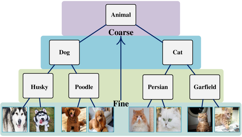
Figure 1. An illustration of a hierarchical semantic structure. Semantic hierarchy is an inherent property of real-world image datasets, e.g., ”image instance $\rightarrow$ husky $\rightarrow$ dog $\rightarrow$ animal” in the order from fine-grained to coarse-grained semantics.

1. Introduction

The explosive growth of multimedia data poses a huge challenge to large-scale information retrieval systems. Hashing-based methods (Cao et al., 2018; Tu et al., 2020; Yuan et al., 2020; Song et al., 2018; Yang et al., 2018; Shen et al., 2020; Wang et al., 2018), converting high-dimensional features to compact binary hash codes while preserving the original similarity information in Hamming space, have become the dominant solution due to their high computation efficiency and low storage cost. Recently, unsupervised hashing methods (Hansen et al., 2021; Song et al., 2018; Yang et al., 2018, 2019; Shen et al., 2020; Qiu et al., 2021; Tu et al., 2020; Li and van Gemert, 2021) have attracted increasing attention since they do not rely on expensive hand-crafted labels and can perceive the distribution of target datasets for real-world retrieval tasks.

Contrastive hashing (Luo et al., 2021; Qiu et al., 2021), as the state-of-the-art unsupervised hashing method, learns hash codes by maximizing the mutual information between different views augmented by an image. However, none of them explores how hierarchical semantics can be used to improve the quality of hash codes, even though the hierarchical semantic structure as an inherent property of image datasets can assist in capturing the latent data distribution. As shown in Figure 1, $Animal$ is a high-level taxon compared to $Dog$. We can obtain a tree-like hierarchical structure with an increasingly coarse semantic granularity from bottom to top. Recently, Lin et al. (Lin et al., 2022) use homology relationships over a two-layer semantic structure to learn hash codes. Although employing the two-layer structure achieves excellent results, there is still room for improvement in constructing and exploiting the hierarchical semantic structures, acquiring more accurate cross-layer affiliation and cross-sample similarity. In addition, embedding the hierarchies into Euclidean or hyper-sphere spaces may miss the optimal solution due to information distortion (Khrulkov et al., 2020; Ermolov et al., 2022; Peng et al., 2021).

To address these problems, we propose constructing hierarchical structures and learning hash codes in hyperbolic space (e.g., the Poincaré ball). Since hyperbolic space has exponential volume growth with respect to the radius (Ermolov et al., 2022; Khrulkov et al., 2020; Peng et al., 2021) and can use low-dimensional manifolds for embeddings without sacrificing the model’s representation power (Nickel and Kiela, 2017a; Ermolov et al., 2022), it results in a lower distortion for embedding hierarchical semantics than Euclidean space with polynomial growth (Sarkar, 2011). To achieve the construction of hierarchical semantic structures in hyperbolic space, we designed the hierarchical hyperbolic K-Means algorithm. The algorithm performs bottom-up clustering with instances over the bottom layer and with prototypes over other layers by the hyperbolic K-Means algorithm, where the hyperbolic K-Means algorithm is our extended K-Means algorithm (MacQueen, 1967) from Euclidean space to hyperbolic space (See $\S$ 3.3). In addition, referring to (Guo et al., 2022), we propose a hierarchical contrastive learning framework for hashing, including hierarchical instance-wise contrastive learning and hierarchical prototype-wise contrastive learning (See $\S$ 3.4). The former leverages hierarchical semantic structures to mine accurate cross-sample similarity, reducing the number of false negatives (Zhang et al., 2022; Cao et al., 2022; Xia et al., 2022) to improve the discriminating ability. The latter aligns the hash codes of image instances with the corresponding prototypes (hash centers (Yuan et al., 2020)) over different layers, mining accurate cross-layer affiliation.

Based on these improvements, we propose a novel unsupervised hashing method called Hyperbolic Hierarchical Contrastive Hashing (HHCH). In the HHCH framework, we learn continuous hash codes and embed them into hyperbolic space with a projection head (See $\S$ 3.2). Meanwhile, we perform hierarchical hyperbolic K-Means over the hyperbolic embeddings to construct hierarchical semantic structures before each training epoch. For hash learning within a mini-batch, we employ the proposed hierarchical contrastive learning under the SimCLR (Chen et al., 2020) framework with the captured hierarchies. Finally, we conducted extensive experiments on four benchmark datasets to verify the superiority of HHCH compared with several state-of-the-art unsupervised hashing methods. The experimental results demonstrate that learning hash codes with the construction, embedding, and exploitation of hierarchical semantic structures in hyperbolic space can significantly improve retrieval performance.

Our main contributions can be outlined as follows:

• We propose a novel contrastive hashing method named HHCH using the proposed hierarchical contrastive learning framework. The framework can benefit from the hierarchical semantic structures to improve the accuracy of cross-sample similarity and cross-layer affiliation for hash learning.

• We propose to project continuous hash codes into hyperbolic space (i.e., the Poincaré ball) for low information distortion. To this end, we designed the hierarchical hyperbolic K-Means algorithm that can work in hyperbolic space and adaptively construct hierarchical semantic structures from bottom to top.

• Extensive experiments on four benchmark datasets demonstrate that HHCH achieves superior retrieval performance compared with several state-of-the-art unsupervised hashing methods.

2. Related Work

Unsupervised Hashing. Existing unsupervised hashing methods mainly fall into two lines: reconstruction-based hashing methods and contrastive hashing methods. The former (Dai et al., 2017; Shen et al., 2020, 2019) mostly adopts an encoder-decoder architecture (Goodfellow et al., 2014; Kingma and Welling, 2014) to reconstruct original images from hash codes and others employ generative adversarial networks to maximize reconstruction likelihood via the discriminator (Song et al., 2018; Zieba et al., 2018; Dizaji et al., 2018). The latter can learn distortion-invariant hash codes, alleviating the problem of background noise caused by the reconstruction process and yielding state-of-the-art performance. Specifically, DATE (Luo et al., 2021) proposes a general distribution-based metric to depict the pairwise distance between images, exploring both semantic-preserving learning and contrastive learning to obtain high-quality hash codes. CIBHash (Qiu et al., 2021) learns hash codes under the SimCLR (Chen et al., 2020) framework and compresses the model by the Information Bottleneck (Tishby and Zaslavsky, 2015). Despite their contributions to learning compact hash codes in an unsupervised manner, they overlook rich information from hierarchical semantic structures inherent to the datasets. DSCH (Lin et al., 2022) is aware of hierarchical semantics and tries to exploit them using homology and co-occurrence relationships mined by its two-step iterative algorithm. There is still room for the exploration of hierarchical semantics. 1) The customized two-layer hierarchical structure can only represent limited hierarchical information. It lacks an effective learning mechanism to adaptively construct hierarchical structures and provide accurate cross-sample and cross-layer information. 2) Embedding the hierarchical semantic structures in hyper-sphere space is not the optimal solution due to information distortion (Khrulkov et al., 2020; Ermolov et al., 2022; Peng et al., 2021).

Hyperbolic Embedding. Recently, hyperbolic embedding technology has been successfully applied to CV (Khrulkov et al., 2020; Ermolov et al., 2022; Yan et al., 2021) and NLP (Nickel and Kiela, 2017b; Dhingra et al., 2018; Tifrea et al., 2019) tasks due to the distinctive property of hyperbolic space, i.e., the exponential volume growth with respect to the radius rather than the polynomial growth in Euclidean space. Although it has been proven to be suitable for embedding hierarchies (e.g., tree graphs) with low distortion (Ermolov et al., 2022; Peng et al., 2021), the algorithm for the construction of hierarchies in hyperbolic space has not been studied. We still need to explore construction schemes for hierarchical information in hyperbolic space for hashing tasks. For more details about hyperbolic embedding, we refer readers to (Peng et al., 2021) for a recent survey.

Contrastive Learning. Contrastive learning learns view-invariant representations by attracting positive samples and repelling negative samples. The instance-wise contrastive learning methods (Chen et al., 2020; He et al., 2020; Grill et al., 2020; Chen and He, 2021), e.g., SimCLR (Chen et al., 2020) and MoCo (He et al., 2020), maximize the identical representation between views augmented from the same instance. They highlight data-data correlations and neglect the global distribution of the whole dataset. To compensate for this, the prototype-wise contrastive learning methods (Li et al., 2021b; Caron et al., 2020; Rosa and Oliveira, 2022; Li et al., 2021a) explicitly exploit the semantic structure and learn the prototypes (i.e., the centers) of each cluster formed by semantically similar instances. Our HHCH benefits from both two kinds of contrastive learning methods as well as recent efforts in hierarchical representation learning (Guo et al., 2022; Xu et al., 2021).

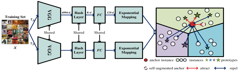
Figure 2. The framework of HHCH. $\tau_{A}$ and $\tau_{B}$ are augmentations used to transform an image. Each transformed view is encoded by VGG and transformed into a $K$-bit continuous hash code. Then, the code is projected into hyperbolic space by a projection head consisting of a fully connected layer and an exponential mapping function. HHCH captures the hierarchical semantic structures before each training epoch and conducts hierarchical contrastive learning to exploit hierarchical information in hyperbolic space. In hierarchical contrastive learning, the anchor sample will contrast with both instances and prototypes at different layers.

3. Methodology

3.1. Problem Definition and Overview

Given a training set $\mathcal{X}=\left\{x_{i}\right\}_{i=1}^{N}$ of $N$ unlabeled images, we aim to learn a nonlinear hash function $f_{\theta_{h}}:x\rightarrow h\in\left\{-1,1\right\}^{K}$ that maps the data from input space $\mathbb{R}^{D}$ to $K$-bit Hamming space. The learning procedure and details of HHCH are shown in Algorithm 1.

In the training phase, given an image $x_{i}$, our proposed $f_{\theta_{h}}$ extracts the feature vector using the VGG model (Simonyan and Zisserman, 2015) and generates the continuous hash code $h_{i}$ through the hash layer. Then, $h_{i}$ is projected to $z_{i}$, i.e., embedding the hash code into hyperbolic space (i.e., the Poincaré ball), with a projection head $Exp\_map_{\theta_{e}}$. The projection head contains a fully-connected layer followed by the exponential mapping function in Equation (3).

Input: Training data $\mathcal{X}$; batch size $B$; Hyper-parameters; Training epochs $T$; Hash function $f_{\theta_{h}}$ and projection head $Exp\_map_{\theta_{e}}$.

Output: Optimized hash function $f_{\theta_{h}}$

Initialize $\bm{\theta_{h}}$ and $\bm{\theta_{e}}$ randomly;

for $t$=1 to $T$ do

       $Z=Exp\_map_{\theta_{e}}(f_{\theta_{h}}(\mathcal{X}))$;

      /* Construct the hierarchical semantic structures and output prototypes $\mathcal{P}$ and connections $\mathcal{E}$. */

       $(\mathcal{P},\mathcal{E})$ $\leftarrow$ Hierarchical hyperbolic K-Means($Z$);

      for $b=1$ to $\frac{N}{B}$ do

            

            $X_{b}^{1}$, $X_{b}^{2}\leftarrow transformation(X_{b})$

            $H_{b}^{1},H_{b}^{2}$=$f_{\theta_{h}}(X_{b}^{1})$, $f_{\theta_{h}}(X_{b}^{2})$

            $Z_{b}^{1},Z_{b}^{2}$=$Exp\_map_{\theta_{e}}(H_{b}^{1})$, $Exp\_map_{\theta_{e}}(H_{b}^{2})$;

            Compute $L_{H-inst}$ and $L_{H-proto}$ with $(Z_{b}^{1},Z_{b}^{2},\mathcal{P},\mathcal{E})$;

            Compute $L_{Q}$ with $(H_{b}^{1},H_{b}^{2})$;

            Compute $\mathcal{L}$ with Equation (16);

            Update $\bm{\theta_{h}}$ and $\bm{\theta_{e}}$ with the Adam optimizer.

      

Algorithm 1 HHCH algorithm.

Before each training epoch, we generate the hyperbolic embeddings $Z=\left\{z_{i}\right\}_{i=1}^{N}$ of all training images and perform hierarchical hyperbolic K-Means to construct hierarchical semantic structures. For the hash learning within the $b$-th mini-batch, we transform every image into two views with various augmentation strategies. Then, we acquire the corresponding hash codes $H_{b}^{1}=\left\{h_{i}^{1}\right\}_{i=1}^{B}$ and $H_{b}^{2}=\left\{h_{i}^{2}\right\}_{i=1}^{B}$ as well as the hyperbolic embeddings $Z_{b}^{1}=\left\{z_{i}^{1}\right\}_{i=1}^{B}$ and $Z_{b}^{2}=\left\{z_{i}^{1}\right\}_{i=1}^{B}$, where $B$ denotes the batch size. Finally, we compute the hierarchical contrastive loss, including the hierarchical instance-wise contrastive loss and the hierarchical prototype-wise contrastive loss, with the hyperbolic embeddings and the captured hierarchies $(\mathcal{P},\mathcal{E})$, where $\mathcal{P}$ is the set of prototypes and $\mathcal{E}$ is the set of connections consisting of prototype-prototype and prototype-instance. In addition, we incorporate the quantization loss to reduce the quantization error.

In the test phase, we only use the well-trained hash function $f_{\theta_{h}}$, disabling the projection head and the hierarchical semantic structures. All the continuous hash codes will be constrained to $\left\{-1,1\right\}^{K}$ by the $sgn$ function for performance evaluation, where $K$ denotes the length of the hash code.

The framework of HHCH is shown in Figure 2. In the following subsections, we will specify HHCH by answering the questions below.

Q1: How can we bridge Euclidean space and hyperbolic space?

Q2: How to construct hierarchical semantic structures in hyperbolic space?

Q3: How to exploit hierarchical semantic structures for hash learning?

3.2. Hyperbolic Space Learning (RQ1)

Formally, $n$-dimensional hyperbolic space $\mathbb{H}^{n}$ is a Riemannian manifold of constant negative curvature rather than the constant positive curvature in Euclidean space. There exist several isomorphic models of hyperbolic space, we specialize in the Poincaré ball model $(\mathbb{D}^{n}_{c},g^{\mathbb{D}})$ with the curvature parameter $c$ (the actual curvature value is then $-c^{2}$) in this work. The model is defined by the manifold $\mathbb{D}^{n}=\{x\in\mathbb{R}^{n}\colon c\|x\|^{2}<1,c\geq 0\}$ endowed with the Riemannian metric $g^{\mathbb{D}}=\lambda_{c}^{2}g^{E}$, where $\lambda_{c}=\frac{2}{1-c\|x\|^{2}}$ is the conformal factor and $g^{E}=\mathbf{I}_{n}$ is the Euclidean metric tensor (Khrulkov et al., 2020; Peng et al., 2021; Ermolov et al., 2022).

Since hyperbolic space is not vector space in a traditional sense, we must introduce the gyrovector formalism (Ungar, 2009) to perform operations such as addition (Khrulkov et al., 2020). As a result, we can define the following operations in Poincaré ball:

Möbius addition. For a pair $\mathbf{x},\mathbf{y}\in\mathbb{D}^{n}_{c}$, their addition is defined below.

(1) $$\mathbf{x}\oplus_{c}\mathbf{y}=\frac{(1+2c\langle\mathbf{x},\mathbf{y}\rangle+c\|\mathbf{y}\|^{2})\mathbf{x}+(1-c\|\mathbf{x}\|^{2})\mathbf{y}}{1+2c\langle\mathbf{x},\mathbf{y}\rangle+c^{2}\|\mathbf{x}\|^{2}\|\mathbf{y}\|^{2}}.$$

Hyperbolic distance. The hyperbolic distance between $\mathbf{x},\mathbf{y}\in\mathbb{D}^{n}_{c}$ is defined below.

(2) $$D_{hyp}(\mathbf{x},\mathbf{y})=\frac{2}{\sqrt{c}}\mathrm{arctanh}(\sqrt{c}\|-\mathbf{x}\oplus_{c}\mathbf{y}\|).$$

Note that with $c\to 0$, the distance function (2) reduces to the Euclidean distance: $\lim_{c\to 0}D_{hyp}(\mathbf{x},\mathbf{y})=2\|\mathbf{x}-\mathbf{y}\|.$

Exponential mapping function. We also need to define a bijective map from Euclidean space to the Poincaré model of hyperbolic geometry. This mapping is termed exponential, while its inverse mapping from hyperbolic space to Euclidean is called logarithmic. For some fixed base point $\mathbf{x}\in\mathbb{D}^{n}_{c}$, the exponential mapping is a function $\exp_{\mathbf{x}}^{c}\colon\mathbb{R}^{n}\to\mathbb{D}_{c}^{n}$ that is defined as follows:

(3) $$\exp_{\mathbf{x}}^{c}(\mathbf{v})=\mathbf{x}\oplus_{c}\bigg{(}\tanh\bigg{(}\sqrt{c}\frac{\lambda_{\mathbf{x}}^{c}\|\mathbf{v}\|}{2}\bigg{)}\frac{\mathbf{v}}{\sqrt{c}\|\mathbf{v}\|}\bigg{)}.$$

Usually, the base point $\mathbf{x}$ is set to $\mathbf{0}$, making the above formulas simple but with little bias to the original results (Ermolov et al., 2022).

In hyperbolic space, the local distances are scaled by the factor $\lambda_{c}$, approaching infinity near the boundary of the ball. As a result, hyperbolic space has the “space expansion property”. While in Euclidean space, the volume of an object with a diameter of $r$ scales polynomially with $r$, in hyperbolic space, the counterpart scales exponentially with $r$. Intuitively, this is a continuous analog of trees: for a tree with a branching factor $k$, we obtain $O(k^{d})$ nodes on level $d$, which in this case serves as a discrete analog of the radius. This property allows us to efficiently embed hierarchical data even in low dimensions, which is made precise by embedding theorems for trees and complex networks (Sarkar, 2011; Ermolov et al., 2022).

3.3. Hierarchical Hyperbolic K-Means (RQ2)

We aim to construct hierarchical structures by capturing hierarchical relationships among semantic clusters in hyperbolic space. To this end, we propose the hierarchical hyperbolic K-Means algorithm in the Poincaré ball, constructing the structures in a bottom-up manner.

The details of hierarchical hyperbolic K-Means are shown in Algorithm 2. We define the number of prototypes at the $l$-th layer as $M_{l}$ and the total number of layers as $L$. First, we obtain the hyperbolic embeddings $Z=\{z_{i}\}_{i=1}^{N}$ of all images before each training epoch. Then, we perform hyperbolic K-Means with $Z$ to obtain the prototypes of the first/bottom layer, i.e., $\{p_{j}^{1}\}_{j=1}^{M_{1}}$. Similarly, the prototypes of each higher layer are derived by iteratively applying hyperbolic K-Means to the prototypes of the layer below (Guo et al., 2022). We record the hierarchical information by maintaining the prototype set $\mathcal{P}=\{\{p_{j}^{l}\}_{j=1}^{M_{l}}\}_{l=1}^{L}$ and the connection set $\mathcal{E}$.

In the above process, the hyperbolic K-Means algorithm is the key to achieving the construction in hyperbolic space. Although the K-Means algorithm optimizes the prototypes and the latent cluster assignments alternatively, existing variants of K-Means define the prototype by the Euclidean averaging operation over all embeddings within the cluster, which does not apply to hyperbolic space. To perform K-Means in hyperbolic space, we have to define 1) the distance metric in hyperbolic space and 2) the calculation of prototypes. The former has been solved in Equation (2). For the latter, we compute the Einstein midpoint as the prototype in hyperbolic space, referring to (Gülçehre et al., 2019), which has the most concise form with the Klein coordinates (Peng et al., 2021; Khrulkov et al., 2020) as follows:

Input: Image hyperbolic embedding $Z$; Number of hierarchies $L$, Number of clusters at the $l$-th hierarchy $M_{l}$.

Output: Hierarchical semantic structures $\left(\mathcal{P},\mathcal{E}\right)$.

$\{p_{j}^{1}\}_{j=1}^{M_{1}}\leftarrow$ Hyperbolic K-Means($Z$)

$\mathcal{E}=\{\left(z_{i},Parent(z_{i})\right)\}_{i=1}^{N}$

for $l$=2 to $L$ do

       $\{p_{j}^{l}\}_{j=1}^{M_{l}}\leftarrow$ Hyperbolic K-Means($\{p_{j}^{l-1}\}_{j=1}^{M_{l-1}}$)

      /* Update connections. $Parent(\cdot)$ means the parent node at a higher level. */

      

      $\mathcal{E}\leftarrow\mathcal{E}\cup\{(p_{j}^{l-1},Parent(p_{i}^{l-1}))\}_{j=1}^{M_{l-1}}$

/* More details about Hyperbolic K-Means */

Initial prototypes using K-Means++ in hyperbolic space with the distance calculated by Equation (2).

while not converged do

      

      calculate cluster assignments according to Equation (2);

      /* The following is the calculation of new prototypes. */

      

      Map all points to the Klein model with Equation (6);

      Compute Einstein midpoints with Equation (4);

      Project all midpoints (prototypes) back to the Poincaré ball;

Algorithm 2 Hierarchical Hyperbolic K-Means.

(4) $$Klein\_Proto(x_{1},...,x_{N})=\sum_{i=1}^{N}\gamma_{i}x_{i}/\sum_{i=1}^{N}\gamma_{i},$$

where $\gamma_{i}=\frac{1}{\sqrt{1-c||x_{i}||^{2}}}$ is the Lorentz factor (Peng et al., 2021). Since the Klein model and the Poincaré ball model are isomorphic (Khrulkov et al., 2020), we can transition between $x_{\mathbb{D}}$ in the Poincaré ball and $x_{\mathbb{K}}$ in the Klein model as follows:

(5) $$x_{\mathbb{K}}=\frac{2x_{\mathbb{D}}}{1+c||x_{\mathbb{D}}||^{2}},$$

(6) $$x_{\mathbb{D}}=\frac{x_{\mathbb{K}}}{1+\sqrt{1-c||x_{\mathbb{K}}||^{2}}}.$$

Based on these formulas, we can map all the points in the Poincaré ball to the Klein model, computing the prototypes via Equation (4) first and then projecting them back to the Poincaré model. As a result, we can conduct hyperbolic K-Means clustering via alternative optimization with the distance metric and the prototype calculation like the existing K-Means algorithms.

3.4. Hierarchical Contrastive Learning (RQ3)

Since the contrastive hashing methods (Qiu et al., 2021; Lin et al., 2022; Luo et al., 2021) have achieved satisfying retrieval performance without hand-crafted labels, we adopt the classic contrastive learning framework SimCLR (Chen et al., 2020) as our fundamental learning framework. To incorporate hierarchical information into the contrastive hashing framework, we propose hierarchical instance-wise contrastive learning and hierarchical prototype-wise contrastive learning, as well as extending them to work in hyperbolic space. We will elaborate on how contrastive hashing benefits from hierarchical semantic structures using both learning patterns.

Hierarchical instance-wise contrastive learning. Instance-wise contrastive learning pushes the embeddings of two transformed views of the same image (positives) close to each other and further apart from the embeddings of other images (negatives), where the instance-wise contrastive loss is defined as follows:

(7) $$\tilde{\ell}_{i}^{1}=-\log\frac{exp\left(-D\left(z_{i}^{1},z_{i}^{2}\right)/\tau\right)}{exp\left(-D\left(z_{i}^{1},z_{i}^{2}\right)/\tau\right)+\sum_{v,z_{n}\in\mathcal{N}(z_{i})}exp\left(-D\left(z_{i}^{1},z_{n}^{v}\right)/\tau\right)},$$

where $z_{i}^{v}$ is the representation of the $v$-th view of $x_{i}$, $\tilde{\ell}_{i}^{v}$ denotes the instance-wise contrastive loss of $z_{i}^{v}$, $\mathcal{N}(z_{i})$ is the negative set of $z_{i}$, $\tau$ is the temperature parameter (Chen et al., 2020; He et al., 2020), and $D$ is the distance metric. We can express $D$ by the cosine distance defined in hyper-sphere space, i.e.,

(8) $$D_{cos}\left(z_{i},z_{j}\right)=\frac{K}{2}\left(1-cos\left(z_{i},z_{j}\right)\right).$$

Similarly, $D$ can be defined as the hyperbolic distance in Equation (2). As a result, the instance-wise contrastive loss for all views of instance $z_{i}$ is formulated as

(9) $$L_{inst}\left(z_{i},\mathcal{N}(z_{i})\right)=\sum_{v=1}^{2}\tilde{\ell}_{i}^{v}.$$

Recent studies show that the selection of negative samples is critical for the quality of contrastive learning (Chen et al., 2020; Zhang et al., 2022; Cao et al., 2022; Xia et al., 2022). Existing contrastive hashing methods (Qiu et al., 2021; Luo et al., 2021; Lin et al., 2022) suffer from the false negative problem (Cao et al., 2022; Xia et al., 2022) since they treat all the remaining images $z_{j}^{v}$ within a mini-batch as negatives when given a random anchor image $z_{i}^{v}$, even if the negative images share the same semantic as the anchor image. We aim to sample distinctive negative samples according to the hierarchical semantic structure, alleviating the problem to achieve a solid discriminating ability for the contrastive hashing model.

Compared to flat structures, hierarchical structures can provide hierarchical similarity based on affiliation, resulting in accurate cross-sample similarity for negative sampling. Specifically, we sample negative samples according to the hierarchical structure constructed in $\S$ 3.3. Given the anchor sample $z_{i}$, the negative sample set $\mathcal{N}^{l}(z_{i})$ at the $l$-th layer can be defined by

(10) $$\mathcal{N}^{l}\left(z_{i}\right)=\left\{z_{j}\mid j=1,...,B\text{ and }\mathcal{P}^{l}(z_{j})\!\neq\!\mathcal{P}^{l}(z_{i})\right\},$$

where $\mathcal{P}^{l}(z_{i})$ is the ancestor of $z_{i}$ at the $l$-th layer. The above equation implies that the negative sample set of the anchor sample $z_{i}$ only contains samples with a different ancestor than $z_{i}$ at the $l$-th layer.

The negative sample sets at different levels in hierarchical contrastive hashing take on varying importance because the granularity of the hierarchical semantic structure decreases from fine to coarse as the level advances. As a result, the overall hierarchical instance-wise contrastive learning objective $\mathcal{L}_{H-inst}$ can be formulated as a weighted summation of contrastive loss in Equation (9) at different layers, i.e.,

(11) $$\mathcal{L}_{H-inst}=\frac{1}{B\cdot L}\sum_{i=1}^{B}\sum_{l=1}^{L}\frac{1}{l}L_{inst}\left(z_{i},\mathcal{N}^{l}(z_{i})\right).$$

Hierarchical prototype-wise contrastive learning. Compared to instance-wise contrastive learning methods (Chen et al., 2020; He et al., 2020; Grill et al., 2020) that learn data-data correlations, contrasting instance-prototype pairs can capture the global data distribution to acquire accurate cross-layer affiliation. To this end, we introduce prototype-wise contrastive learning (Li et al., 2021b), where we define the ancestor $\mathcal{P}^{l}(z_{i})$ of $z_{i}$ as the positive sample and all the remaining prototypes as negative samples. Analogous to Equation (7), the prototype-wise contrastive loss is defined below.

(12) $$\hat{\ell}_{i}^{v}\!\!=-\!\log\!\frac{exp\left(-\!D\left(z_{i}^{v},\mathcal{P}(z_{i})\right)\!/\tau\right)}{exp\left(-\!D\left(z_{i}^{v},\mathcal{P}(z_{i})\right)\!/\tau\right)\!+\!\!\sum_{p_{n}\in\mathcal{N}_{p}(z_{i})}\!exp\left(-\!D(z_{i}^{v},p_{n})\!/\tau\right)},$$

where $N_{p}(z_{i})$ is the negative prototypes set of $z_{i}$ and $p_{n}\in N_{p}(z_{i})$. The prototype-wise contrastive loss for all views can be defined as follows:

(13) $$L_{proto}(z_{i},\mathcal{N}_{p}(z_{i}))=\sum_{v=1}^{2}\hat{\ell}_{i}^{v}.$$

We employ a different negative sampling strategy for the hierarchical prototype-wise contrastive learning than for the hierarchical instance-wise learning for two reasons. On the one hand, since negative prototypes are usually distinct from the anchor image, prototype-wise contrastive learning suffers less from the false negative problem than instance-wise contrastive learning. On the other hand, since the number of prototypes is much less than the number of instances, the negative sampling strategy for hierarchical instance-wise contrastive learning will cause the problem of under-sampling for negatives in hierarchical prototype-wise contrastive learning.

By contrasting prototypes at different layers, we define the hierarchical prototype-wise contrastive loss as follows:

(14) $$\mathcal{L}_{H-proto}=\frac{1}{B\cdot L}\sum_{i=1}^{B}\sum_{l=1}^{L}\frac{1}{l}L_{proto}\left(z_{i},\mathcal{N}_{p}^{l}(z_{i})\right).$$

In addition, referring to (Zhu et al., 2016), we define the quantization loss to reduce the accumulated quantization error caused by the continuous relaxation, where the loss is defined below.

(15) $$\mathcal{L}_{Q}=\frac{1}{2}\sum_{i=1}^{B}\sum_{k=1}^{K}\sum_{v=1}^{2}\left(\log cosh(|h_{i,k}^{v}|-\mathbf{1})\right),$$

where $h_{i,k}$ is the $k$-th bit of $h_{i}$ and $\mathbf{1}\in\mathbb{R}^{K}$ is the vector of ones. Finally, the overall learning objective of hierarchical contrastive hashing can be formulated as follows:

(16) $$\mathcal{L}=\mathcal{L}_{H-inst}+\mathcal{L}_{H-proto}+\lambda\mathcal{L}_{Q}.$$

where $\lambda$ is the hyper-parameter to trade off different loss items.

Table 1. Comparison in mAP of Hamming Ranking for different bits on image retrieval.

Method	Reference	ImageNet			CIFAR-10			FLICKR25K			NUS-WIDE
		16-bit	32-bit	64-bit	16-bit	32-bit	64-bit	16-bit	32-bit	64-bit	16-bit	32-bit	64-bit
SGH (Dai et al., 2017)	ICML17	0.557	0.572	0.583	0.286	0.320	0.347	0.608	0.657	0.693	0.463	0.588	0.638
SSDH (Yang et al., 2018)	IJCAI18	0.604	0.619	0.631	0.241	0.239	0.256	0.710	0.696	0.737	0.542	0.629	0.635
BGAN (Song et al., 2018)	AAAI18	0.649	0.665	0.675	0.535	0.575	0.587	0.766	0.770	0.795	0.719	0.745	0.761
DistillHash (Yang et al., 2019)	CVPR19	0.654	0.671	0.683	0.547	0.582	0.591	0.779	0.793	0.801	0.722	0.749	0.762
ML$S^{3}$RDUH (Tu et al., 2020)	IJCAI20	0.662	0.680	0.691	0.562	0.588	0.595	0.797	0.809	0.809	0.730	0.754	0.764
TBH (Shen et al., 2020)	CVPR20	0.636	0.653	0.667	0.432	0.459	0.455	0.779	0.794	0.797	0.678	0.717	0.729
CIBHash (Qiu et al., 2021)	IJCAI21	0.719	0.733	0.747	0.547	0.583	0.602	0.773	0.781	0.798	0.756	0.777	0.781
DSCH (Lin et al., 2022)	AAAI22	0.749	0.761	0.774	0.624	0.644	0.670	0.817	0.827	0.828	0.770	0.792	0.801
HHCH	Ours	0.783	0.814	0.826	0.631	0.657	0.681	0.825	0.838	0.842	0.797	0.820	0.828

4. Experiments

In this section, we conduct experiments on four public benchmark datasets to evaluate the superiority of our proposed HHCH. More detailed experimental results and additional visualizations can be found in the supplementary material. Note that baseline results are reported from DSCH (Lin et al., 2022).

4.1. Dataset and Evaluation Metrics

The public benchmark datasets include ImageNet (Deng et al., 2009), CIFAR-10 (Krizhevsky et al., 2009), FLICKR25K (Huiskes and Lew, 2008), and NUS-WIDE (Chua et al., 2009).

ImageNet is a commonly used single-label image dataset. Following (Yuan et al., 2020; Cao et al., 2017, 2018), we randomly select 100 categories for the experiments. Besides, we use 5,000 images as the query set and the remaining images as the retrieval set, where we randomly select 100 images per category as the training set.

CIFAR-10 consists of 60,000 images containing 10 classes. We follow the common setting (Lin et al., 2022) and select 1,000 images (100 per class) as the query set. The remaining images are used as the retrieval set, where we randomly selected 1,000 images per class to form the training set.

NUS-WIDE is a multi-label dataset that contains 269,648 images from 81 classes. Following the commonly used setting (Lin et al., 2022; Qiu et al., 2021; Shen et al., 2020), we only use images selected from 21 most frequent classes. Besides, we sample 100 images per class as the query set and use the remaining as the retrieval set, where we randomly select 10,500 images (5,00 images per class) to form the training set.

FLICKR25K is a multi-label dataset containing 25,000 images from 24 categories. Following (Lin et al., 2022), we randomly sample 1,000 images as the query set, and the remaining images are left for the retrieval set. In the retrieval set, we randomly choose 10,000 images as the training set.

Evaluation Protocol. To evaluate retrieval quality, we follow (Shen et al., 2020; Yuan et al., 2020; Shen et al., 2019; Tu et al., 2020, 2021) to employ the following metrics: 1) Mean Average Precision (mAP), 2) Precision-Recall (P-R) curves, 3) Precision curves w.r.t. different numbers of returned samples (P@N), 4) Precision curves within Hamming radius 2 (P@H$\leq$2), 5) Mean intra-class distance $d_{intra}$, and 6) Mean inter-class distance $d_{inter}$. According to (Qiu et al., 2021; Shen et al., 2020), we adopt mAP@1000 for ImageNet and CIFAR-10, as well as mAP@5000 for FLICKR25K and NUS-WIDE.

Table 2. The $d_{intra}$ and $d_{inter}$ on ImageNet.

Method	$d_{intra}\downarrow$			$d_{inter}\uparrow$
	16-bit	32-bit	64-bit	16-bit	32-bit	64-bit
CIBHash	1.23	2.54	5.12	8.04	16.08	32.16
DSCH	1.03	2.24	4.59	8.06	16.12	32.24
HHCH (Ours)	0.81	1.88	3.88	8.08	16.15	32.31

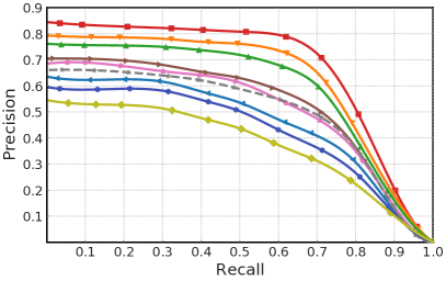
(a) P-R curve at ImageNet:64bits

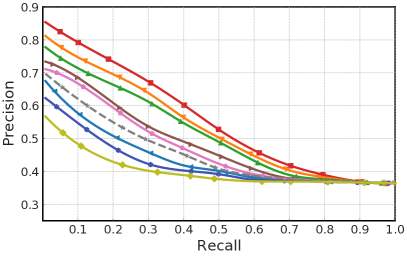
(b) P-R curve at NUS-WIDE:64bits

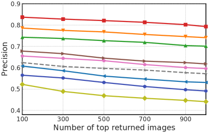
(c) P@N=5000 at ImageNet:64bits

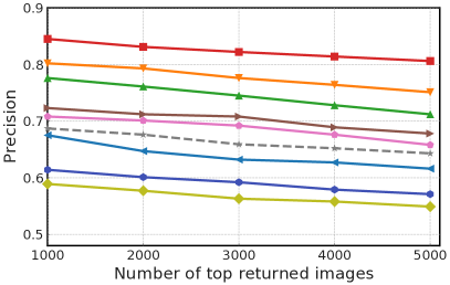
(d) P@N=5000 at NUS-WIDE:64bits

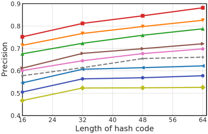
(e) P@H$\leq$2 on ImageNet

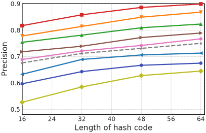
(f) P@H$\leq$2 on NUS-WIDE

Figure 3. P-R curves, P@N, and P@H$\leq$2 of HHCH and comparison methods on ImageNet and NUS-WIDE.

4.2. Implementation Details

Model details. For fair comparisons, we follow DSCH (Lin et al., 2022) to adopt VGG19 (Simonyan and Zisserman, 2015) pre-trained on ImageNet (Deng et al., 2009) as the backbone, and use the hash layer consisting of two fully-connected layers with $ReLU$ as the activation function for hash code projection (Lin et al., 2022). The $3\times 224\times 224$ image will be transformed to a $4096-d$ feature vector and then to the $K$-bit continuous hash code. In addition, we have an auxiliary projection head $Exp\_map$ parameterized by $\theta_{e}$ after the hash layer. The $K$-bit hash code will finally be projected to a 128-bit hyperbolic embedding in the Poincaré ball.

Training details. We implement HHCH in PyTorch (Paszke et al., 2019) and train the model with an NVIDIA RTX 3090 GPU. Following (Qiu et al., 2021; Shen et al., 2019, 2020), we freeze the backbone and only train the hash layer and the projection head. For data augmentation, we use the same strategy as CIBHash (Qiu et al., 2021) and DSCH (Lin et al., 2022). We set the curvature parameter $c=0.1$ for ImageNet and $c=0.01$ for other datasets (See $\S$ 4.5). The temperature parameter $\tau=0.2$ (Equations (7) and (12)). The default $M$ and $L$ are set to $[1500\rightarrow 1000\rightarrow 800]$ for ImageNet, $[100\rightarrow 80\rightarrow 50]$ for CIFAR-10, $[200\rightarrow 150\rightarrow 80]$ for FLICKR25K, and $[200\rightarrow 150\rightarrow 80]$ for NUS-WIDE (See $\S$ 4.5 for detailed investigation with different clustering settings). We set the batch size $B=64$ and adopt the Adam optimizer (Kingma and Ba, 2015) with a learning rate $lr=0.001$.

4.3. Comparison and Analysis

The mAP results on four benchmark datasets are shown in Table 1. It is clear that our proposed HHCH consistently achieves the best retrieval performance among the four image datasets, with an average increase of $4.5\%$, $1.6\%$, $1.3\%$, and $3.5\%$ on ImageNet, CIFAR-10, FLICKR25K, and NUS-WIDE compared with DSCH, respectively. We also report the mean intra-class distance $d_{intra}$ and mean inter-class distance $d_{inter}$ on ImageNet in Table 2. The results demonstrate that HHCH can learn more compact hash codes with greater disentangling ability than others. In addition, we report the P-R curves, P@N curves, and P@H$\leq 2$ curves at 64 bits in Figure 3. Obviously, HHCH outperforms all compared methods by large margins on both ImageNet and FLICKR25K w.r.t. the three metrics. These comparisons imply that HHCH can generate high-quality hash codes, leading to stable superior retrieval performance.

4.4. Ablation Study

To justify how each component of HHCH contributes to final retrieval performance, we conduct studies on the effectiveness of 1) the embedding of hash codes into hyperbolic space and 2) the utilization of hierarchical semantic structures.

Effect of hyperbolic embedding. We report the mAP performance of embedding in hyper-sphere space and hyperbolic space in Table 2. In hyper-sphere space, we disable the projection head, perform hierarchical K-Means directly on the continuous hash codes, and use Equation (8) as the distance metric to compute the contrastive loss. We observe that hyperbolic embedding can boost an average increase of $2.7\%$ and $1.6\%$ on ImageNet and FLICKR25K, respectively, which implies that hyperbolic space has superior expression ability with less distortion than hyper-sphere space.

Effect of hierarchical semantic structures. Table 4 reports the mAP results under different settings of hierarchical semantic structures. IC and PC denote the baseline models using instance-wise contrastive learning and prototype-wise contrastive learning, respectively. They have no perception of latent hierarchical semantic structures, resulting in sub-optimal retrieval performance. Comparing the third and first row of Table 4, we can observe respective $3.4\%$ and $1.5\%$ performance gains on ImageNet and NUS-WIDE after adding the hierarchical information to the instance-wise contrastive learning. This result verifies that hierarchies can effectively help instance-wise contrastive learning to sample more accurate negative samples and mine more accurate cross-sample similarity. In addition, comparing the fourth and second row of Table 4, we can achieve respective $4.2\%$ and $2.0\%$ performance improvements on ImageNet and NUS-WIDE when employing prototype-wise contrastive learning with hierarchies. It demonstrates that accurate cross-layer affiliation provided by hierarchical semantic structures is beneficial to contrastive hashing. Finally, HIC+HPC achieves the best performance, demonstrating that HHCH consisting of both hierarchical instance-wise contrastive learning and hierarchical prototype-wise contrastive learning promises the full utilization of the hierarchical information from both local and global perspectives.

Table 3. The mAP performance in different embedding space.

Space	ImageNet			NUS-WIDE
	16-bit	32-bit	64-bit	16-bit	32-bit	64-bit
Hyper-sphere	0.769	0.791	0.798	0.790	0.806	0.811
Hyperbolic	0.783	0.814	0.826	0.797	0.820	0.828

Table 4. Ablation studies on hierarchical semantic structures. IC: instance-wise contrastive learning without hierarchies; HIC: hierarchical instance-wise contrastive learning; PC: prototype-wise contrastive learning without hierarchies; HPC: hierarchical prototype-wise contrastive learning.

Setting	ImageNet			NUS-WIDE
	16-bit	32-bit	64-bit	16-bit	32-bit	64-bit
IC	0.735	0.758	0.763	0.755	0.781	0.789
PC	0.729	0.747	0.758	0.744	0.777	0.784
HIC	0.755	0.784	0.795	0.768	0.787	0.805
HPC	0.750	0.782	0.798	0.761	0.788	0.802
HIC+HPC	0.783	0.814	0.826	0.797	0.820	0.828

4.5. Sensitivity Analysis

In this section, we give a detailed analysis of the hyper-parameters in the model training phase, including the $M_{l}$ and $L$ of the hierarchical hyperbolic K-Means, the curvature parameter $c$ of the hyperbolic space, and the trade-off parameter $\lambda$. Since parameters like the batch size $B$ and the temperature parameter $\tau$, etc., have been analyzed in the related works (Chen et al., 2020; Qiu et al., 2021), we do not experiment on these parameters.

Sensitivity to $M_{l}$ and $L$. We test the model’s performance with a variation of the number of layers and the number of prototypes at each layer. As shown in Table 5, we can draw the following conclusions: 1) Deeper hierarchies can improve the retrieval performance. Compared with learning with only one layer, HHCH achieves $2.5\%$ and $4.3\%$ improvement on ImageNet and NUS-WIDE under the best settings, respectively. Nevertheless, the depth of the hierarchy is not linearly related to performance. There exists a trade-off between performance and computation overhead. 2) HHCH relies on sufficient prototypes to fully capture the latent distribution. In the setting of a three-level hierarchy, more prototypes bring more performance improvements. Similarly, excessive prototypes do not improve performance.

Table 5. Sensitivity analysis on the number of layers $L$ and the number of prototypes at different layers $M_{l}$. We present the configuration of $M_{l}$ and $L$ as $M_{1}\rightarrow M_{2}\rightarrow...,\rightarrow M_{L}$.

Dataset	Configuration of $M_{l}$ and $L$	mAP@64-bit
ImageNet	500	0.789
	1500	0.806
	$1500\rightarrow 1000$	0.817
	$2000\rightarrow 1500\rightarrow 800$	0.825
	$1500\rightarrow 1000\rightarrow 800$	0.826
	$1000\rightarrow 800\rightarrow 500$	0.822
	$1500\rightarrow 1000\rightarrow 800\rightarrow 500$	0.824
NUS-WIDE	100	0.798
	200	0.794
	$200\rightarrow 150$	0.817
	$300\rightarrow 120\rightarrow 100$	0.826
	$200\rightarrow 150\rightarrow 80$	0.828
	$100\rightarrow 80\rightarrow 50$	0.822
	$200\rightarrow 150\rightarrow 80\rightarrow 40$	0.827

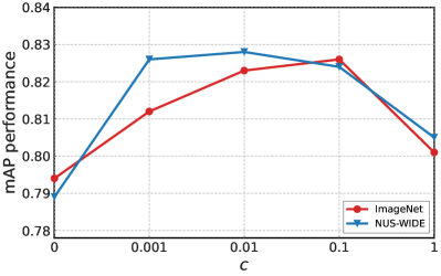
(a) Curvature parameter $c$

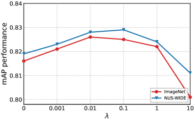
(b) Trade-off parameter $\lambda$

Figure 4. The mAP performance w.r.t. different $c$ and $\lambda$ at 64 bits on ImageNet and NUS-WIDE.

Sensitivity to $c$. We investigate the effect of the curvature parameter $c$. Intuitively, the smaller $c$ is, the flatter the Poincaré ball is. As shown in Figure 4 (a), mAP increases as $c$ at the beginning. It gets a peak value at $c=0.01$ or $c=0.1$ but drops off sharply after $c=0.1$. In addition, we find that the optimal mAP for ImageNet is higher than that for NUS-WDIE. We attribute it to the clear hierarchical semantic structures of the ImageNet dataset that are organized according to the WordNet (Miller, 1995) hierarchy.

Sensitivity to $\lambda$. We test the model’s performance depending on the trade-off parameter $\lambda$ at 64 bits on ImageNet and NUS-WIDE. As shown in Figure 4 (b), we can observe that both small and large $\lambda$ will decrease the mAP performance. A small $\lambda$ can not reduce the accumulated quantization error caused by the continuous relaxation, resulting in considerable information loss. In contrast, a large $\lambda$ will force the quantization loss item to dominate the overall learning objective, resulting in the difficulty of optimization. As a result, we opt for $\lambda=0.01$.

4.6. Visualization

Hash Codes Visualization. Figure 5 shows the t-SNE visualization (van der Maaten and Hinton, 2008) of the hash codes at 64 bits on CIFAR-10 and ImageNet. The hash codes generated by HHCH show favorable intra-class compactness and inter-class separability compared with the state-of-the-art hashing method DSCH. It demonstrates that HHCH can generate high-quality hash codes.

Hyperbolic Embeddings Visualization. We illustrate the hyperbolic embeddings of CIFAR-10 and ImageNet in the Poincaré ball using UMAP (McInnes et al., 2018) with the “hyperboloid” distance metric (Ermolov et al., 2022). We can see that the samples are clustered according to the labels, and each cluster is pushed to the border of the ball, indicating that the learned embeddings are distinguishable enough.

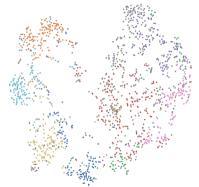
(a) CIFAR-10:DSCH

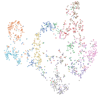
(b) CIFAR-10:HHCH

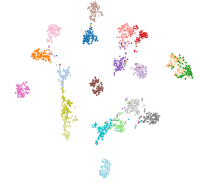
(c) ImageNet:DSCH

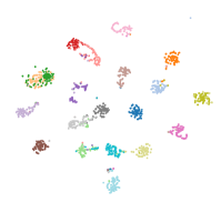
(d) ImageNet:HHCH

Figure 5. The t-SNE visualization of the learned 64-bit hash codes from the training sets. The scattered elements of the same color indicate the same category. Note that we only visualize the first 20 classes for ImageNet.

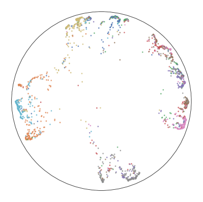
(a) CIFAR-10

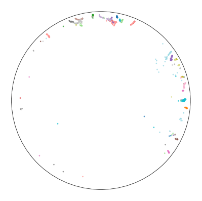
(b) ImageNet

Figure 6. The UMAP visualization of 128-d hyperbolic embeddings from ImageNet (The first 20 classes) and CIFAR-10 in the Poincaré ball.

5. Conclusion

In this paper, we propose to learn hash codes by exploiting the hierarchical semantic structures that naturally exist in real-world datasets. As a result, we proposed a novel unsupervised hashing method named HHCH. In HHCH, we embed the continuous hash codes into hyperbolic space (i.e., the Poincaré ball) to achieve less information distortion. Furthermore, we extend the K-Means algorithm to hyperbolic space and perform hierarchical hyperbolic K-Means to capture the latent hierarchical semantic structures adaptively. In addition, we designed hierarchical contrastive learning, including hierarchical instance-wise contrastive learning and hierarchical prototype-wise contrastive learning, to take full advantage of the hierarchies. Extensive experiments on four benchmarks demonstrate that HHCH can benefit from the hierarchies and outperforms the state-of-the-art unsupervised methods.

Appendix

Appendix A More details about the framework

Figure 2 shows the framework of HHCH. Following SimCLR (Chen et al., 2020), we adopt Siamese networks directly sharing parameters as our learning framework. We first augment the training images with a combination of different augmentation strategies to generate various views of the same image. The augmentation strategies include random crop, color jittering, Gaussian blur, etc. We can feed the $224\times 224\times 3$-d images to the VGG19 (Simonyan and Zisserman, 2015) backbone, and obtain the $4096$-d feature vectors. Then, we employ the hash layer, including two fully-connected layers with the ReLU function as the activation function, to transform them into $K$-d features. Furthermore, all these features will be constrained to $(-1,1)$ via the $tanh$ function for continuous relaxation. After that, the projection head, consisting of a fully connected layer and the exponential mapping function, will map all the continuous hash codes into the hyperbolic space (i.e., the Poincaré ball) with the hyperbolic embedding dimension of 128, where we perform hierarchical contrastive learning with the captured hierarchical semantic structures.

In the test phase, we disable the projection head and generate hash codes with the VGG backbone and the well-trained hash layer. We use the modified $sgn$ function for binarization:

(17) $$sgn(h_{k})=\begin{cases}-1,&\text{if }h_{k}\leq 0,\\ 1,&otherwise,\end{cases}$$

where $h_{k}$ is the $k$-th bit of the hash code $h$.

Appendix B More details about datasets

The details of the dataset setting can be found in Table 6. For ImageNet and NUS-WIDE, we follow (Yuan et al., 2020; Cao et al., 2018) to use the commonly adopted index files and compressed datasets from the repository of HashNet (Cao et al., 2017) to form the splits. Besides, we follow (Li and van Gemert, 2021) to implement CIFAR-10 and FLICKR25K.

Table 6. Experimental settings for all datasets.

Dataset	#Train	#Query	#Retrieval	#Class
ImageNet	1,3000	5,000	128,503	100
CIFAR-10	10,000	1,000	59,000	10
FLICKR25K	10,000	1,000	24,000	24
NUS-WIDE	10,500	2,100	193,734	21

Appendix C Top-10 Retrieved Results

Figure 8 illustrates the top-10 retrieved images and reports P@10 comparisons between HHCH and DSCH (Lin et al., 2022). Our proposed HHCH achieves $90\%$ and $100\%$ in terms of P@10 when given the query images labeled as “Norfolk terrier” and “Sky&Clouds” on ImageNet and NUS-WIDE, respectively. It can be seen that our proposed HHCH yields more relevant and accurate retrieval results than DSCH.

Appendix D Visualization of Hierarchical Semantics

In Figure 7, we visualize the partial results of the hierarchical hyperbolic K-Means. It is clear that images at low layers express finer-grained semantics and the high layers contain coarser-grained semantics, e.g., images at the bottom of the hierarchy are naturally more visually similar, while the images at the top of the hierarchy are more diverse. These results indicate that HHCH is capable of capturing the hierarchical semantics of the data very well.

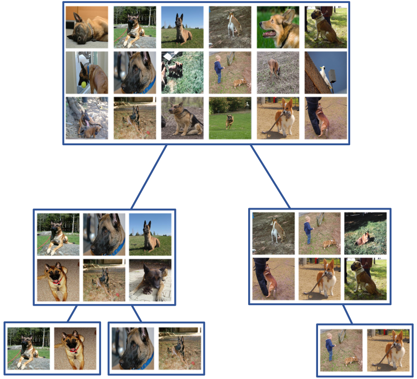
Figure 7. Visualization of a captured hierarchical semantic structure. Note that we only use a small part of the images for the visualization.

Appendix E Time Complexity Analysis

Since HHCH involves an extra hierarchical hyperbolic K-Means algorithm before each epoch for the training phase, we discuss the possible extra time overhead according to time complexity. Note that $N$, $M_{l}$, $L$, and $B$ denote the dataset size, number of prototypes at the $l$-th layer, number of layers, and the mini-batch size, respectively.

On the one hand, the time complexity of vanilla K-Means is $\mathcal{O}(NMt)$, where $t$ is the number of iterations in K-Means and we set $t=30$. For hierarchical hyperbolic K-Means, the extra time complexity of each training step is $\mathcal{O}(NM_{1}t+M_{1}M_{2}t+...+M_{L-1}M_{L}t)/(N/B)$. Since $M_{l}\ll N$, we can simplify it to $\mathcal{O}(BM_{1}t)$.

On the other hand, the time complexity of hierarchical instance-wise contrastive learning is $\mathcal{O}(B^{2})$, and the counterpart of hierarchical prototype-wise contrastive learning is $\mathcal{O}(BM_{1}+...+BM_{L})=\mathcal{O}(BM_{1})$. As a result, the time complexity of hierarchical contrastive loss computation is $\mathcal{O}(B^{2})+\mathcal{O}(BM_{1})$.

In conclusion, the complete time complexity of HHCH is $\mathcal{O}(B^{2})+\mathcal{O}(BM_{1})+\mathcal{O}(BM_{1}t)=\mathcal{O}(BM_{1}t)$, which is consistent with state-of-the-art contrastive hashing methods DSCH (Lin et al., 2022) but a little higher than CIBHash (Qiu et al., 2021) when $M_{1}t>B$.

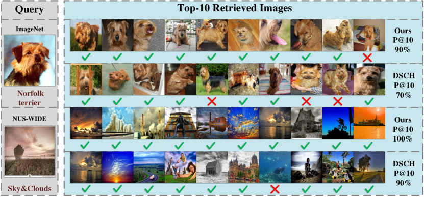
Figure 8. Retrieval comparisons to DSCH (Lin et al., 2022) at 64 bits on three datasets. The Top-10 retrieved images are returned according to the Hamming distance between the query image and the database images. We report precision within the top-10 retrieved images (P@10) and the results demonstrate that our proposed HHCH outperforms DSCH with more relevant and accurate returned images as well as fewer contradictions.

References

- (1)
- Cao et al. (2022) Rui Cao, Yihao Wang, Yuxin Liang, Ling Gao, Jie Zheng, Jie Ren, and Zheng Wang. 2022. Exploring the Impact of Negative Samples of Contrastive Learning: A Case Study of Sentence Embedding. In Findings of the Association for Computational Linguistics: ACL 2022, Dublin, Ireland, May 22-27, 2022, Smaranda Muresan, Preslav Nakov, and Aline Villavicencio (Eds.). Association for Computational Linguistics, 3138–3152.
- Cao et al. (2018) Yue Cao, Mingsheng Long, Bin Liu, and Jianmin Wang. 2018. Deep Cauchy Hashing for Hamming Space Retrieval. In 2018 IEEE Conference on Computer Vision and Pattern Recognition, CVPR 2018, Salt Lake City, UT, USA, June 18-22, 2018. Computer Vision Foundation / IEEE Computer Society, 1229–1237.
- Cao et al. (2017) Zhangjie Cao, Mingsheng Long, Jianmin Wang, and Philip S. Yu. 2017. HashNet: Deep Learning to Hash by Continuation. In IEEE International Conference on Computer Vision, ICCV 2017, Venice, Italy, October 22-29, 2017. IEEE Computer Society, 5609–5618.
- Caron et al. (2020) Mathilde Caron, Ishan Misra, Julien Mairal, Priya Goyal, Piotr Bojanowski, and Armand Joulin. 2020. Unsupervised Learning of Visual Features by Contrasting Cluster Assignments. (2020).
- Chen et al. (2020) Ting Chen, Simon Kornblith, Mohammad Norouzi, and Geoffrey E. Hinton. 2020. A Simple Framework for Contrastive Learning of Visual Representations. In Proceedings of the 37th International Conference on Machine Learning, ICML 2020, 13-18 July 2020, Virtual Event (Proceedings of Machine Learning Research, Vol. 119). PMLR, 1597–1607.
- Chen and He (2021) Xinlei Chen and Kaiming He. 2021. Exploring Simple Siamese Representation Learning. In IEEE Conference on Computer Vision and Pattern Recognition, CVPR 2021, virtual, June 19-25, 2021. Computer Vision Foundation / IEEE, 15750–15758.
- Chua et al. (2009) Tat-Seng Chua, Jinhui Tang, Richang Hong, Haojie Li, Zhiping Luo, and Yantao Zheng. 2009. NUS-WIDE: a real-world web image database from National University of Singapore. In Proceedings of the 8th ACM International Conference on Image and Video Retrieval, CIVR 2009, Santorini Island, Greece, July 8-10, 2009, Stéphane Marchand-Maillet and Yiannis Kompatsiaris (Eds.). ACM.
- Dai et al. (2017) Bo Dai, Ruiqi Guo, Sanjiv Kumar, Niao He, and Le Song. 2017. Stochastic Generative Hashing. In Proceedings of the 34th International Conference on Machine Learning, ICML 2017, Sydney, NSW, Australia, 6-11 August 2017 (Proceedings of Machine Learning Research, Vol. 70), Doina Precup and Yee Whye Teh (Eds.). PMLR, 913–922.
- Deng et al. (2009) Jia Deng, Wei Dong, Richard Socher, Li-Jia Li, Kai Li, and Li Fei-Fei. 2009. ImageNet: A large-scale hierarchical image database. In 2009 IEEE Computer Society Conference on Computer Vision and Pattern Recognition (CVPR 2009), 20-25 June 2009, Miami, Florida, USA. IEEE Computer Society, 248–255.
- Dhingra et al. (2018) Bhuwan Dhingra, Christopher J. Shallue, Mohammad Norouzi, Andrew M. Dai, and George E. Dahl. 2018. Embedding Text in Hyperbolic Spaces. In Proceedings of the Twelfth Workshop on Graph-Based Methods for Natural Language Processing, TextGraphs@NAACL-HLT 2018, New Orleans, Louisiana, USA, June 6, 2018, Goran Glavas, Swapna Somasundaran, Martin Riedl, and Eduard H. Hovy (Eds.). Association for Computational Linguistics, 59–69.
- Dizaji et al. (2018) Kamran Ghasedi Dizaji, Feng Zheng, Najmeh Sadoughi, Yanhua Yang, Cheng Deng, and Heng Huang. 2018. Unsupervised Deep Generative Adversarial Hashing Network. In 2018 IEEE Conference on Computer Vision and Pattern Recognition, CVPR 2018, Salt Lake City, UT, USA, June 18-22, 2018. Computer Vision Foundation / IEEE Computer Society, 3664–3673.
- Ermolov et al. (2022) Aleksandr Ermolov, Leyla Mirvakhabova, Valentin Khrulkov, Nicu Sebe, and Ivan V. Oseledets. 2022. Hyperbolic Vision Transformers: Combining Improvements in Metric Learning. CoRR abs/2203.10833 (2022). arXiv:2203.10833
- Goodfellow et al. (2014) Ian J. Goodfellow, Jean Pouget-Abadie, Mehdi Mirza, Bing Xu, David Warde-Farley, Sherjil Ozair, Aaron C. Courville, and Yoshua Bengio. 2014. Generative Adversarial Nets. (2014), 2672–2680.
- Grill et al. (2020) Jean-Bastien Grill, Florian Strub, Florent Altché, Corentin Tallec, Pierre H. Richemond, Elena Buchatskaya, Carl Doersch, Bernardo Ávila Pires, Zhaohan Guo, Mohammad Gheshlaghi Azar, Bilal Piot, Koray Kavukcuoglu, Rémi Munos, and Michal Valko. 2020. Bootstrap Your Own Latent - A New Approach to Self-Supervised Learning. (2020).
- Gülçehre et al. (2019) Çaglar Gülçehre, Misha Denil, Mateusz Malinowski, Ali Razavi, Razvan Pascanu, Karl Moritz Hermann, Peter W. Battaglia, Victor Bapst, David Raposo, Adam Santoro, and Nando de Freitas. 2019. Hyperbolic Attention Networks. In 7th International Conference on Learning Representations, ICLR 2019, New Orleans, LA, USA, May 6-9, 2019. OpenReview.net.
- Guo et al. (2022) Yuanfan Guo, Minghao Xu, Jiawen Li, Bingbing Ni, Xuanyu Zhu, Zhenbang Sun, and Yi Xu. 2022. HCSC: Hierarchical Contrastive Selective Coding. CoRR abs/2202.00455 (2022). arXiv:2202.00455
- Hansen et al. (2021) Christian Hansen, Casper Hansen, Jakob Grue Simonsen, Stephen Alstrup, and Christina Lioma. 2021. Unsupervised Multi-Index Semantic Hashing. In WWW ’21: The Web Conference 2021, Virtual Event / Ljubljana, Slovenia, April 19-23, 2021, Jure Leskovec, Marko Grobelnik, Marc Najork, Jie Tang, and Leila Zia (Eds.). ACM / IW3C2, 2879–2889.
- He et al. (2020) Kaiming He, Haoqi Fan, Yuxin Wu, Saining Xie, and Ross B. Girshick. 2020. Momentum Contrast for Unsupervised Visual Representation Learning. In 2020 IEEE/CVF Conference on Computer Vision and Pattern Recognition, CVPR 2020, Seattle, WA, USA, June 13-19, 2020. Computer Vision Foundation / IEEE, 9726–9735.
- Huiskes and Lew (2008) Mark J. Huiskes and Michael S. Lew. 2008. The MIR flickr retrieval evaluation. In Proceedings of the 1st ACM SIGMM International Conference on Multimedia Information Retrieval, MIR 2008, Vancouver, British Columbia, Canada, October 30-31, 2008, Michael S. Lew, Alberto Del Bimbo, and Erwin M. Bakker (Eds.). ACM, 39–43. https://doi.org/10.1145/1460096.1460104
- Khrulkov et al. (2020) Valentin Khrulkov, Leyla Mirvakhabova, Evgeniya Ustinova, Ivan V. Oseledets, and Victor S. Lempitsky. 2020. Hyperbolic Image Embeddings. In 2020 IEEE/CVF Conference on Computer Vision and Pattern Recognition, CVPR 2020, Seattle, WA, USA, June 13-19, 2020. Computer Vision Foundation / IEEE, 6417–6427.
- Kingma and Ba (2015) Diederik P. Kingma and Jimmy Ba. 2015. Adam: A Method for Stochastic Optimization. In 3rd International Conference on Learning Representations, ICLR 2015, San Diego, CA, USA, May 7-9, 2015, Conference Track Proceedings, Yoshua Bengio and Yann LeCun (Eds.).
- Kingma and Welling (2014) Diederik P. Kingma and Max Welling. 2014. Auto-Encoding Variational Bayes. (2014).
- Krizhevsky et al. (2009) Alex Krizhevsky, Geoffrey Hinton, et al. 2009. Learning multiple layers of features from tiny images. (2009).
- Li et al. (2021b) Junnan Li, Pan Zhou, Caiming Xiong, and Steven C. H. Hoi. 2021b. Prototypical Contrastive Learning of Unsupervised Representations. (2021).
- Li et al. (2021a) Yunfan Li, Peng Hu, Jerry Zitao Liu, Dezhong Peng, Joey Tianyi Zhou, and Xi Peng. 2021a. Contrastive Clustering. In Thirty-Fifth AAAI Conference on Artificial Intelligence, AAAI 2021, Thirty-Third Conference on Innovative Applications of Artificial Intelligence, IAAI 2021, The Eleventh Symposium on Educational Advances in Artificial Intelligence, EAAI 2021, Virtual Event, February 2-9, 2021. AAAI Press, 8547–8555.
- Li and van Gemert (2021) Yunqiang Li and Jan van Gemert. 2021. Deep Unsupervised Image Hashing by Maximizing Bit Entropy. In Thirty-Fifth AAAI Conference on Artificial Intelligence, AAAI 2021, Thirty-Third Conference on Innovative Applications of Artificial Intelligence, IAAI 2021, The Eleventh Symposium on Educational Advances in Artificial Intelligence, EAAI 2021, Virtual Event, February 2-9, 2021. AAAI Press, 2002–2010.
- Lin et al. (2022) Qinghong Lin, Xiaojun Chen, Qin Zhang, Shaotian Cai, Wenzhe Zhao, and Hongfa Wang. 2022. Deep Unsupervised Hashing with Latent Semantic Components. In Thirty-Sixth AAAI Conference on Artificial Intelligence, AAAI 2022, Thirty-Fourth Conference on Innovative Applications of Artificial Intelligence, IAAI 2022, The Twelveth Symposium on Educational Advances in Artificial Intelligence, EAAI 2022 Virtual Event, February 22 - March 1, 2022. AAAI Press, 7488–7496.
- Luo et al. (2021) Xiao Luo, Daqing Wu, Zeyu Ma, Chong Chen, Minghua Deng, Jianqiang Huang, and Xian-Sheng Hua. 2021. A Statistical Approach to Mining Semantic Similarity for Deep Unsupervised Hashing. In MM ’21: ACM Multimedia Conference, Virtual Event, China, October 20 - 24, 2021, Heng Tao Shen, Yueting Zhuang, John R. Smith, Yang Yang, Pablo Cesar, Florian Metze, and Balakrishnan Prabhakaran (Eds.). ACM, 4306–4314.
- MacQueen (1967) J. MacQueen. 1967. Some methods for classification and analysis of multivariate observations.
- McInnes et al. (2018) Leland McInnes, John Healy, Nathaniel Saul, and Lukas Großberger. 2018. UMAP: Uniform Manifold Approximation and Projection. J. Open Source Softw. 3, 29 (2018), 861.
- Miller (1995) George A Miller. 1995. WordNet: a lexical database for English. Commun. ACM 38, 11, 39–41.
- Nickel and Kiela (2017a) Maximilian Nickel and Douwe Kiela. 2017a. Poincaré Embeddings for Learning Hierarchical Representations. In Advances in Neural Information Processing Systems 30: Annual Conference on Neural Information Processing Systems 2017, December 4-9, 2017, Long Beach, CA, USA, Isabelle Guyon, Ulrike von Luxburg, Samy Bengio, Hanna M. Wallach, Rob Fergus, S. V. N. Vishwanathan, and Roman Garnett (Eds.). 6338–6347.
- Nickel and Kiela (2017b) Maximilian Nickel and Douwe Kiela. 2017b. Poincaré Embeddings for Learning Hierarchical Representations. In Advances in Neural Information Processing Systems 30: Annual Conference on Neural Information Processing Systems 2017, December 4-9, 2017, Long Beach, CA, USA, Isabelle Guyon, Ulrike von Luxburg, Samy Bengio, Hanna M. Wallach, Rob Fergus, S. V. N. Vishwanathan, and Roman Garnett (Eds.). 6338–6347.
- Paszke et al. (2019) Adam Paszke, Sam Gross, Francisco Massa, Adam Lerer, James Bradbury, Gregory Chanan, Trevor Killeen, Zeming Lin, Natalia Gimelshein, Luca Antiga, Alban Desmaison, Andreas Köpf, Edward Z. Yang, Zachary DeVito, Martin Raison, Alykhan Tejani, Sasank Chilamkurthy, Benoit Steiner, Lu Fang, Junjie Bai, and Soumith Chintala. 2019. PyTorch: An Imperative Style, High-Performance Deep Learning Library. In Advances in Neural Information Processing Systems 32: Annual Conference on Neural Information Processing Systems 2019, NeurIPS 2019, December 8-14, 2019, Vancouver, BC, Canada, Hanna M. Wallach, Hugo Larochelle, Alina Beygelzimer, Florence d’Alché-Buc, Emily B. Fox, and Roman Garnett (Eds.). 8024–8035.
- Peng et al. (2021) Wei Peng, Tuomas Varanka, Abdelrahman Mostafa, Henglin Shi, and Guoying Zhao. 2021. Hyperbolic Deep Neural Networks: A Survey. CoRR abs/2101.04562 (2021). arXiv:2101.04562
- Qiu et al. (2021) Zexuan Qiu, Qinliang Su, Zijing Ou, Jianxing Yu, and Changyou Chen. 2021. Unsupervised Hashing with Contrastive Information Bottleneck. In Proceedings of the Thirtieth International Joint Conference on Artificial Intelligence, IJCAI 2021, Virtual Event / Montreal, Canada, 19-27 August 2021, Zhi-Hua Zhou (Ed.). ijcai.org, 959–965.
- Rosa and Oliveira (2022) Laura Elena Cué La Rosa and Dário Augusto Borges Oliveira. 2022. Learning from Label Proportions with Prototypical Contrastive Clustering. In Thirty-Sixth AAAI Conference on Artificial Intelligence, AAAI 2022, Thirty-Fourth Conference on Innovative Applications of Artificial Intelligence, IAAI 2022, The Twelveth Symposium on Educational Advances in Artificial Intelligence, EAAI 2022 Virtual Event, February 22 - March 1, 2022. AAAI Press, 2153–2161.
- Sarkar (2011) Rik Sarkar. 2011. Low Distortion Delaunay Embedding of Trees in Hyperbolic Plane. In Graph Drawing - 19th International Symposium, GD 2011, Eindhoven, The Netherlands, September 21-23, 2011, Revised Selected Papers (Lecture Notes in Computer Science, Vol. 7034), Marc J. van Kreveld and Bettina Speckmann (Eds.). Springer, 355–366.
- Shen et al. (2019) Yuming Shen, Li Liu, and Ling Shao. 2019. Unsupervised Binary Representation Learning with Deep Variational Networks. Int. J. Comput. Vis. 127, 11-12, 1614–1628.
- Shen et al. (2020) Yuming Shen, Jie Qin, Jiaxin Chen, Mengyang Yu, Li Liu, Fan Zhu, Fumin Shen, and Ling Shao. 2020. Auto-Encoding Twin-Bottleneck Hashing. In 2020 IEEE/CVF Conference on Computer Vision and Pattern Recognition, CVPR 2020, Seattle, WA, USA, June 13-19, 2020. Computer Vision Foundation / IEEE, 2815–2824.
- Simonyan and Zisserman (2015) Karen Simonyan and Andrew Zisserman. 2015. Very Deep Convolutional Networks for Large-Scale Image Recognition. (2015). http://arxiv.org/abs/1409.1556
- Song et al. (2018) Jingkuan Song, Tao He, Lianli Gao, Xing Xu, Alan Hanjalic, and Heng Tao Shen. 2018. Binary Generative Adversarial Networks for Image Retrieval. In Proceedings of the Thirty-Second AAAI Conference on Artificial Intelligence, (AAAI-18), the 30th innovative Applications of Artificial Intelligence (IAAI-18), and the 8th AAAI Symposium on Educational Advances in Artificial Intelligence (EAAI-18), New Orleans, Louisiana, USA, February 2-7, 2018, Sheila A. McIlraith and Kilian Q. Weinberger (Eds.). AAAI Press, 394–401.
- Tifrea et al. (2019) Alexandru Tifrea, Gary Bécigneul, and Octavian-Eugen Ganea. 2019. Poincare Glove: Hyperbolic Word Embeddings. In 7th International Conference on Learning Representations, ICLR 2019, New Orleans, LA, USA, May 6-9, 2019. OpenReview.net.
- Tishby and Zaslavsky (2015) Naftali Tishby and Noga Zaslavsky. 2015. Deep learning and the information bottleneck principle. In 2015 IEEE Information Theory Workshop, ITW 2015, Jerusalem, Israel, April 26 - May 1, 2015. IEEE, 1–5.
- Tu et al. (2021) Rong-Cheng Tu, Xian-Ling Mao, Jia-Nan Guo, Wei Wei, and Heyan Huang. 2021. Partial-Softmax Loss based Deep Hashing. In WWW ’21: The Web Conference 2021, Virtual Event / Ljubljana, Slovenia, April 19-23, 2021, Jure Leskovec, Marko Grobelnik, Marc Najork, Jie Tang, and Leila Zia (Eds.). ACM / IW3C2, 2869–2878.
- Tu et al. (2020) Rong-Cheng Tu, Xianling Mao, and Wei Wei. 2020. MLS3RDUH: Deep Unsupervised Hashing via Manifold based Local Semantic Similarity Structure Reconstructing. In Proceedings of the Twenty-Ninth International Joint Conference on Artificial Intelligence, IJCAI 2020, Christian Bessiere (Ed.). ijcai.org, 3466–3472.
- Ungar (2009) Abraham Albert Ungar. 2009. A Gyrovector Space Approach to Hyperbolic Geometry. Morgan & Claypool Publishers.
- van der Maaten and Hinton (2008) Laurens van der Maaten and Geoffrey E. Hinton. 2008. Visualizing Data using t-SNE. Journal of Machine Learning Research 9 (2008), 2579–2605.
- Wang et al. (2018) Jingdong Wang, Ting Zhang, Jingkuan Song, Nicu Sebe, and Heng Tao Shen. 2018. A Survey on Learning to Hash. IEEE Trans. Pattern Anal. Mach. Intell. 40, 4 (2018), 769–790.
- Xia et al. (2022) Jun Xia, Lirong Wu, Ge Wang, Jintao Chen, and Stan Z. Li. 2022. ProGCL: Rethinking Hard Negative Mining in Graph Contrastive Learning. In International Conference on Machine Learning, ICML 2022, 17-23 July 2022, Baltimore, Maryland, USA (Proceedings of Machine Learning Research, Vol. 162), Kamalika Chaudhuri, Stefanie Jegelka, Le Song, Csaba Szepesvári, Gang Niu, and Sivan Sabato (Eds.). PMLR, 24332–24346.
- Xu et al. (2021) Minghao Xu, Hang Wang, Bingbing Ni, Hongyu Guo, and Jian Tang. 2021. Self-supervised Graph-level Representation Learning with Local and Global Structure. In Proceedings of the 38th International Conference on Machine Learning, ICML 2021, 18-24 July 2021, Virtual Event (Proceedings of Machine Learning Research, Vol. 139), Marina Meila and Tong Zhang (Eds.). PMLR, 11548–11558.
- Yan et al. (2021) Jiexi Yan, Lei Luo, Cheng Deng, and Heng Huang. 2021. Unsupervised Hyperbolic Metric Learning. In IEEE Conference on Computer Vision and Pattern Recognition, CVPR 2021, virtual, June 19-25, 2021. Computer Vision Foundation / IEEE, 12465–12474.
- Yang et al. (2018) Erkun Yang, Cheng Deng, Tongliang Liu, Wei Liu, and Dacheng Tao. 2018. Semantic Structure-based Unsupervised Deep Hashing. In Proceedings of the Twenty-Seventh International Joint Conference on Artificial Intelligence, IJCAI 2018, July 13-19, 2018, Stockholm, Sweden, Jérôme Lang (Ed.). ijcai.org, 1064–1070.
- Yang et al. (2019) Erkun Yang, Tongliang Liu, Cheng Deng, Wei Liu, and Dacheng Tao. 2019. DistillHash: Unsupervised Deep Hashing by Distilling Data Pairs. In IEEE Conference on Computer Vision and Pattern Recognition, CVPR 2019, Long Beach, CA, USA, June 16-20, 2019. Computer Vision Foundation / IEEE, 2946–2955.
- Yuan et al. (2020) Li Yuan, Tao Wang, Xiaopeng Zhang, Francis E. H. Tay, Zequn Jie, Wei Liu, and Jiashi Feng. 2020. Central Similarity Quantization for Efficient Image and Video Retrieval. In 2020 IEEE/CVF Conference on Computer Vision and Pattern Recognition, CVPR 2020, Seattle, WA, USA, June 13-19, 2020. Computer Vision Foundation / IEEE, 3080–3089.
- Zhang et al. (2022) Yanzhao Zhang, Richong Zhang, Samuel Mensah, Xudong Liu, and Yongyi Mao. 2022. Unsupervised Sentence Representation via Contrastive Learning with Mixing Negatives. In Thirty-Sixth AAAI Conference on Artificial Intelligence, AAAI 2022, Thirty-Fourth Conference on Innovative Applications of Artificial Intelligence, IAAI 2022, The Twelveth Symposium on Educational Advances in Artificial Intelligence, EAAI 2022 Virtual Event, February 22 - March 1, 2022. AAAI Press, 11730–11738.
- Zhu et al. (2016) Han Zhu, Mingsheng Long, Jianmin Wang, and Yue Cao. 2016. Deep Hashing Network for Efficient Similarity Retrieval. In Proceedings of the Thirtieth AAAI Conference on Artificial Intelligence, February 12-17, 2016, Phoenix, Arizona, USA, Dale Schuurmans and Michael P. Wellman (Eds.). AAAI Press, 2415–2421.
- Zieba et al. (2018) Maciej Zieba, Piotr Semberecki, Tarek El-Gaaly, and Tomasz Trzcinski. 2018. BinGAN: Learning Compact Binary Descriptors with a Regularized GAN. In Advances in Neural Information Processing Systems 31: Annual Conference on Neural Information Processing Systems 2018, NeurIPS 2018, December 3-8, 2018, Montréal, Canada, Samy Bengio, Hanna M. Wallach, Hugo Larochelle, Kristen Grauman, Nicolò Cesa-Bianchi, and Roman Garnett (Eds.). 3612–3622.