Exactly Solvable Spin Tri-Junctions

Abstract

We present a class of exactly solvable tri-junctions of one- and two-dimensional spin systems. Based on the geometric criterion for solvability, we clarify the sufficient condition for the junctions so that the spin Hamiltonian becomes equivalent to Majorana quadratic forms. Then we examine spin tri-junctions using the obtained solvable models. We consider the transverse magnetic field Ising spin chains and reveal how Majorana zero modes appear at the tri-junctions of the chains. Local terms of the tri-junction crucially affect the appearance of Majorna zero modes, and the tri-junction may support Majorana zero mode even if the bulk spin chains do not have Majorna end states. We also examine tri-junctions of two-dimensional SO(5)-spin lattices and discuss Majorana fermions along the junctions.

I Introduction

The Jordan-Wigner transformation (JWT) Jordan and Wigner (1928) maps spin operators into fermion ones. In the context of lower-dimensional exactly solvable models, the JWT has played an important role because this transformation helps solve a class of spin systems exactly Onsager (1944); Kaufman (1949); Kaufman and Onsager (1949); Nambu (1995); Lieb et al. (1961); Niemeijer (1967); Katsura (1962); Pfeuty (1970); Shankar and Murthy (1987); Minami (2016, 2017). For example, the JWT converts the transverse field Ising model or the one-dimensional (1D) XY model into a bi-linear of Majorana fermions, i.e., a Majorana quadratic form(MQF), enabling us to precisely calculate these models’ spectra, partition functions, phase transitions, and so on.

Whereas recent attempts have explored the generalization of fermionization in higher-dimensional spin systems Kitaev (2006); Kitaev and Laumann (2009); Ryu (2009); Wu et al. (2009); Bochniak and Ruba (2020); Bochniak et al. (2020); Po (2021); Li and Po (2022); Minami (2019); Nussinov and Ortiz (2009); Cobanera et al. (2011); Nussinov et al. (2012); Chen and Kapustin (2019); Chen (2020); Fendley (2019); Chapman and Flammia (2020); Prosko et al. (2017); Yu and Wang (2008); Lee et al. (2007); Shi et al. (2009), the critical difference from the low-dimensional JWT is that it generally brings additional $\mathbb{Z}_{2}$ gauge fields. For example, a $\mathbb{Z}_{2}$ gauge field accompanies the MQF of the Kitaev spin model in the honeycomb lattice, which originates from redundancy in the Majorana representation of the spin variables $\mathbb{Z}_{2}$. Nonetheless, the model’s ground state is solvable and reveals interesting quantum spin liquid phases.

In our previous paper Ogura et al. (2020), we developed a method unifying the above two techniques, which we call the single-point-connected simplicial complex (SPSC) method. The SPSC method gives a simple criterion for the solvability of lattice spin systems, based on the graph theory and the simplicial homology. Compared with the above two techniques, the SPSC method has three merits: First, it allows us to understand fermionization visually. Second, $\mathbb{Z}_{2}$ gauge degrees of freedom naturally emerge. Finally, this method covers many known solvable spin models and systematically gives novel ones. For example, it solves the transverse field Ising model, the XY model, and the Kitaev honeycomb spin lattice on equal footing. Moreover, we can construct new solvable spin models in higher dimensions or fractals.

In this paper, as a continuation of our previous paper, we construct exactly solvable spin junctions using the SPSC method. In particular, we examine the condition for the appearance of Majorana junction modes in exactly solvable spin tri-junctions of one- and two-dimensional spin systems. Such junctions naturally generalize boundary problems in spin systems, and recent experiments enable their fabrication, but they have rarely been studied systematically.

The rest of this paper is organized as follows. In Sec. II, we briefly review the SPSC method to construct exactly solvable models. In Sec. III, we present a class of exactly solvable tri-junctions of spin chains. We consider tri-junctions of the transverse field Ising chains and obtain the spectra. We reveal that local terms of tri-junctions significantly affect the presence of Majorana zero modes on the junctions. In Sec. IV, we generalize the argument in Sec.III to tri-junctions of two-dimensinal $SO(5)$-spin lattices. Finally, we give a discussion in Sec. V.

II SPSC method

In this section, we summarize the main results of the SPSC method. See Ref. Ogura et al. (2020) for detailed discussions and the proofs of theorems below. For the graph theory and simplicial homology theory, see also Refs. Godsil and Royle (2001); Bondy and Murty (2008), and Kozlov (2008); Nakahara (2003), respectively.

We start with a Hamiltonian $H$, which satisfies the following properties:

(a) $H$ has the form of $H=\sum_{j=1}^{n}\lambda_{j}h_{j}$ where $\lambda_{j}$’s are the real coefficients and $h_{j}$’s are operators.

(b) The operators $h_{j}$ satisfy

$$h_{j}^{\dagger}=h_{j},\quad h_{j}^{2}=1,\quad h_{j}h_{k}=\eta_{j,k}h_{j}h_{k},$$ (1)

where $\eta_{j,k}=\pm 1$.

From these operators $h_{1},\ldots,h_{n}$, we construct the commutativity graph (CG) of the Hamiltonian $H$ as follows:

(a) Put $n$ vertices in general position and place $h_{j}$ on the $j$-th vertex.

(b) When $\eta_{j,k}=-1$ ($\eta_{j,k}=1$), we draw (do not draw) an edge between $j$-th and $k$-th vertices.

Below, $\mathop{\mathrm{CG}}(H)$ denotes this graph. Note that if $\mathop{\mathrm{CG}}(H)$ is not connected, the Hamiltonian is divided into several parts that commute with each other. Since these parts are diagonalizable separately, we consider only the connected $\mathop{\mathrm{CG}}(H)$ without losing the generality.

A special class of simplicial complexes called single-point-connected simplicial complexes (SPSCs) is defined as follows. Let $S_{1},\ldots,S_{m}$ be simplices, and $V$ be a set consisting of all vertices in $S_{1},\ldots,S_{m}$. Then the set of these simplices $\{S_{1},\ldots,S_{m}\}$ are called single-point-connected if the following conditions are satisfied:

(a) If $S_{\alpha}\cap S_{\beta}\neq\emptyset$, $S_{\alpha}\cap S_{\beta}=\{v\}$ holds for some $v\in V$.

(b) For each vertex $v\in V$, exactly two simplices in $\{S_{1},\ldots,S_{m}\}$ include $v$.

The following simplicial complex under this condition

$$K(S_{1},\ldots,S_{m}):=\bigcup_{\alpha=1}^{m}\left\{s\subset S_{\alpha}\mathrel{}\middle|\mathrel{}\text{$s$ is a face of $S_{\alpha}$}\right\}$$ (2)

defines an SPSC. An example is described in Fig. 1.

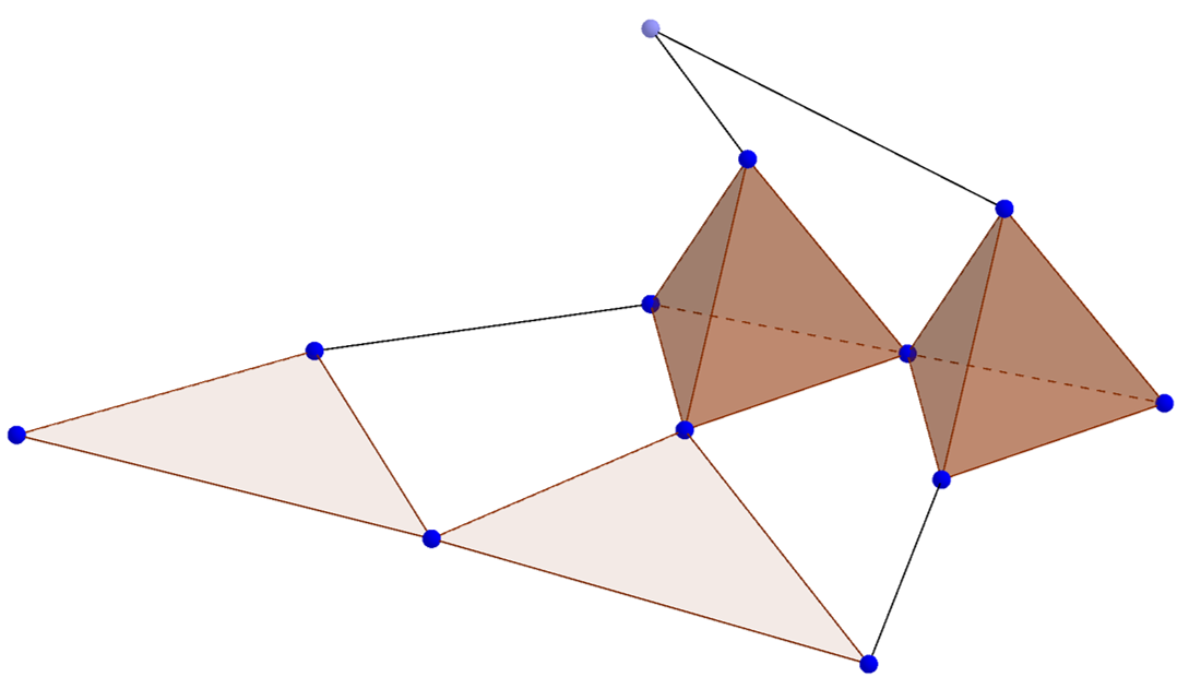
Figure 1: An example of an SPSC. This SPSC has $12$ vertices and $10$ generating simplices (two 3-simplices, two 2-simplices, four 1-simplices, and two 0-simplices.) Hence the dimension of its first homology group becomes $3$ by Theorem 2, which corresponds to the number of holes in it.

For a simplicial complex $K$, we also define the flame $\mathop{\mathrm{Fr}}(K)$ of $K$ as a graph whose vertices and edges are $0$-faces and $1$-faces in $K$, respectively.

Under the above preparation, we introduce an SPSC Hamiltonian. We call the Hamiltonian $H$ an SPSC Hamiltonian for $K$, if there exists an SPSC $K=K(S_{1},\ldots,S_{m})$ obeying $\mathop{\mathrm{Fr}}(K)=\mathop{\mathrm{CG}}(H)$. Now we explain the main theorem:

Theorem 1.

Let $H=\sum_{j=1}^{n}\lambda_{j}h_{j}$ be an SPSC Hamiltonian for a connected SPSC $K=K(S_{1},\ldots,S_{m})$. Then $H$ is mapped to a quadratic form of $m$ Majorana operators $\varphi_{1},\ldots,\varphi_{m}$ that are put on the simplices $S_{1},\ldots,S_{m}$, respectively. More precisely, if the $j$-th vertex is shared by $S_{\alpha}$ and $S_{\beta}$, $h_{j}$ is described as

$$h_{j}=-i\epsilon_{j}\varphi_{\alpha}\varphi_{\beta},$$ (3)

where $\epsilon_{j}=\pm 1$.

The sign factors $\epsilon_{j}$ above can be regarded as a $\mathbb{Z}_{2}$ gauge field and are determined as follows. Using the $\mathbb{Z}_{2}$ gauge transformation $\varphi_{\alpha}\to-\varphi_{\alpha}$, we can change the sign factor $\epsilon_{j}$ in Eq. (3) without changing (anti-)commutation relations of $h_{j}$s. While this procedure trivializes $m-1$ relative signs, $n-m+1$ sign factors remain unfixed. For the unfixed sign factors, we have the next theorem. .

Theorem 2.

Under the same assumption of Theorem 1,

$$\dim H_{1}(K;\mathbb{Z}_{2})=n-m+1$$ (4)

holds, i.e., there exist $n-m+1$ holes in $K$. Correspondingly, we obtain $n-m+1$ conserved quantities from $h_{j}$s on these holes, determining the unfixed sign factors.

From these two theorems, we can solve various spin systems exactly in terms of free fermion systems with $\mathbb{Z}_{2}$ gauge fields $\epsilon_{j}$ Ogura et al. (2020).

III Tri-Junctions of 1D spin chains

In this section, we construct exactly solvable tri-junctions of one-dimensional (1D) spin chains and examine their properties.

III.1 Transverse Field Ising Model

Before discussing junction models, we solve the transverse field Ising chain by the SPSC method. The Hamiltonian of the transverse field Ising chain reads

$$H=-J\sum_{j=1}^{\infty}\sigma^{z}(j)\sigma^{z}(j+1)-h\sum_{j=2}^{\infty}\sigma^{x}(j)-t\sigma^{x}(1),$$ (5)

where $\sigma^{z}(j)$ and $\sigma^{x}(j)$ are the $z$- and $x$-components of the Pauli matrices at site $j$, $J$ is the exchange constant, $h$ is the transverse magnetic field, and $t$ is a magnetic field at the endpoint of the chain. Assigning $h(j)$ as $h(1)=\sigma^{z}(1)$ and

$$h(2j)=\sigma^{z}(j)\sigma^{x}(j+1),\quad h(2j+1)=\sigma^{x}(j+1),$$ (6)

for $j=1,2,\dots$, we have the CG in Fig. 2.

Figure 2: The CG of the transverse field Ising chain.

Regarding each edge and vertex in the CG as a 1-simplex and a 0-simplex, we can identify the CG as an SPSC. Since there is no hole in the CG, the corresponding Hamiltonian with the Majorana operator $\varphi(j)$ reads

$$H= it\varphi(0)\varphi(1)+iJ\sum_{j=1}^{\infty}\varphi(2j-1)\varphi(2j)$$

$$+ih\sum_{j=1}^{\infty}\varphi(2j)\varphi(2j+1),$$ (7)

where we fix the $\mathbb{Z}_{2}$ gauge field as $+1$ by the gauge transformation. We represent this Hamiltonian in the matrix form,

$$H=\frac{i}{2}\vec{\varphi}^{\dagger}\mathcal{A}\vec{\varphi},$$ (8)

where

$$\vec{\varphi} =\begin{pmatrix}\varphi(0)&\varphi(1)&\varphi(2)&\varphi(3)&\cdots\end{pmatrix}^{T},$$

$$\mathcal{A} =\begin{pmatrix}0&t&&&&\\ -t&0&J&&&\\ &-J&0&h&&\\ &&-h&0&\ddots&\\ &&&\ddots&\ddots\end{pmatrix}.$$ (9)

For an eigenvalue $\lambda$ of $\mathcal{A}$ with an eigenvector

$$\vec{v}=\begin{pmatrix}v(0)&w(0)&v(1)&w(1)&\cdots\end{pmatrix}^{T},$$ (10)

the eigenequation is given by

$$tw(0) =\lambda v(0),$$ (11)

$$-tv(0)+Jv(1) =\lambda w(0),$$ (12)

$$-Jw(n-1)+hw(n) =\lambda v(n),$$ (13)

$$-hv(n)+Jv(n+1) =\lambda w(n),$$ (14)

with $n=1,2,\ldots$. Note that the eigenvalue $\lambda$ gives an energy $E$ of the system by $E=i\lambda$.

To solve the eigenequation, we define the generating functions:

$$V(z)=\sum_{n=1}^{\infty}v(n)z^{n},\quad W(z)=\sum_{n=1}^{\infty}w(n)z^{n}.$$ (15)

Then from Eqs. (12), (13) and (14), we get

$$\begin{pmatrix}\lambda&Jz-h\\ h-Jz^{-1}&\lambda\end{pmatrix} \begin{pmatrix}V(z)\\ W(z)\end{pmatrix}$$

$$=v(0) \begin{pmatrix}0\\ -t\end{pmatrix}+w(0)\begin{pmatrix}-Jz\\ -\lambda\end{pmatrix}.$$ (16)

Thus, $V(z)$ and $W(z)$ are given by

$$V(z)= \frac{1}{hJ}\frac{z}{z^{2}-2\kappa z+1}$$

$$\times\left[t\left(h-Jz\right)v(0)+h\lambda w(0)\right],$$

$$W(z)= \frac{1}{hJ}\frac{z}{z^{2}-2\kappa z+1}$$

$$\times\left[t\lambda v(0)-(J^{2}+\lambda^{2}-hJz)w(0)\right],$$ (17)

where

$$\kappa:=\frac{J^{2}+h^{2}+\lambda^{2}}{2Jh}.$$ (18)

Now we examine the spectrum of this Hamiltonian. Let $z_{\pm}$ be the roots of $z^{2}-2\kappa z+1$. Since they satisfy

$$z_{+}+z_{-}=2\kappa,\quad z_{+}z_{-}=1,$$ (19)

we have

$$\frac{z}{z^{2}-2\kappa z+1} =\frac{1}{z_{+}-z_{-}}\left(\frac{z_{+}z}{1-z_{+}z}-\frac{z_{-}z}{1-z_{-}z}\right)$$

$$=\sum_{n=1}^{\infty}\left(\frac{z_{+}^{n}-z_{-}^{n}}{z_{+}-z_{-}}\right)z^{n}.$$ (20)

We require $|z_{\pm}|=1$ in order to obtain the bulk spectrum. Setting $z_{\pm}=e^{ik}$ with $k\in(-\pi,\pi]$, then from Eq. (19), we obtain the bulk spectrum as

$$E=\pm\sqrt{J^{2}+h^{2}-2Jh\cos k}\quad(k\in(-\pi,\pi]),$$ (21)

which reproduces the result in Ref. Minami (2016). Remark that the bulk spectrum becomes gapless if $J=h$ holds.

In contrast, for $|z_{\pm}|\neq 1$, we have boundary modes. We focus on zero energy boundary modes with $\lambda=0$, then from Eq. (III.1), we obtain

$$V(z)=\frac{tz}{J-hz}v(0)=\frac{t}{h}v(0)\sum_{n=1}^{\infty}\left(\frac{hz}{J}\right)^{n},$$

$$W(z)=\frac{Jz}{h-Jz}w(0)=w(0)\sum_{n=1}^{\infty}\left(\frac{Jz}{h}\right)^{n}.$$ (22)

Moreover, we also get $w(0)=0$ from Eq. (11), which implies $W(z)=0$. So the boundary state becomes

$$v(0)\cdot\begin{pmatrix}1&0&\frac{t}{h}\cdot\frac{h}{J}&0&\frac{t}{h}\cdot\left(\frac{h}{J}\right)^{2}&0&\cdots\end{pmatrix}^{T},$$ (23)

which satisfies the $L^{2}$ condition for $h<J$. Therefore, under this condition, a zero energy boundary state appears.

In summary, we find a phase transition at $J=h$, and the transverse field Ising chain supports a zero energy boundary state for $h<J$.

III.2 Exactly Solvable Spin Tri-junctions

In this subsection, we discuss patterns of spin tri-junctions considered in this paper. We consider tri-junctions of the transverse field Ising chains, of which Hamiltonian is given by

$$H =\sum_{\mu=1}^{3}H_{\mu}^{\mathrm{bulk}}+H^{\mathrm{junc}}.$$ (24)

Here $H_{\mu}^{\mathrm{bulk}}$ is the semi-infinite bulk spin chain Hamiltonian

$$H_{\mu}^{\mathrm{bulk}}$$

$$=-\sum_{\mu=1}^{3}\left[J_{\mu}\sum_{j=1}^{\infty}\sigma_{\mu}^{z}(j)\sigma_{\mu}^{z}(j+1)+h_{\mu}\sum_{j=2}^{\infty}\sigma_{\mu}^{x}(j)\right],$$ (25)

with the index $\mu=1,2,3$ specifying the chains. Like Eq. (6), we assign $h_{\mu}(j)$ as

$$h_{\mu}(2j)=\sigma_{\mu}^{z}(j)\sigma_{\mu}^{z}(j+1),\quad h_{\mu}(2j+1)=\sigma_{\mu}^{x}(j+1),$$

$$(j=1,2,\dots).$$ (26)

Below, we determine the junction part $H^{\mathrm{junc}}$ so that the CG of $H$ becomes an SPSC. We do not treat a junction

$$H^{\mathrm{junc}}= -\sum_{\mu=1}^{3}h_{\mu}\sigma_{\mu}^{x}(1)-g_{12}\sigma_{1}^{z}(1)\sigma_{2}^{z}(1)$$

$$-g_{23}\sigma_{2}^{z}(1)\sigma_{3}^{z}(1)-g_{31}\sigma_{3}^{z}(1)\sigma_{1}^{z}(1),$$ (27)

with the interchain couplings $g_{\mu\nu}$ Tsvelik (2013); Giuliano et al. (2016, 2020). From the assignment, $h_{\mu,\nu}(0)=\sigma_{\mu}^{z}(1)\sigma_{\nu}^{z}(1),$ we obtain the CG in Fig. 3, but this is not an SPSC.

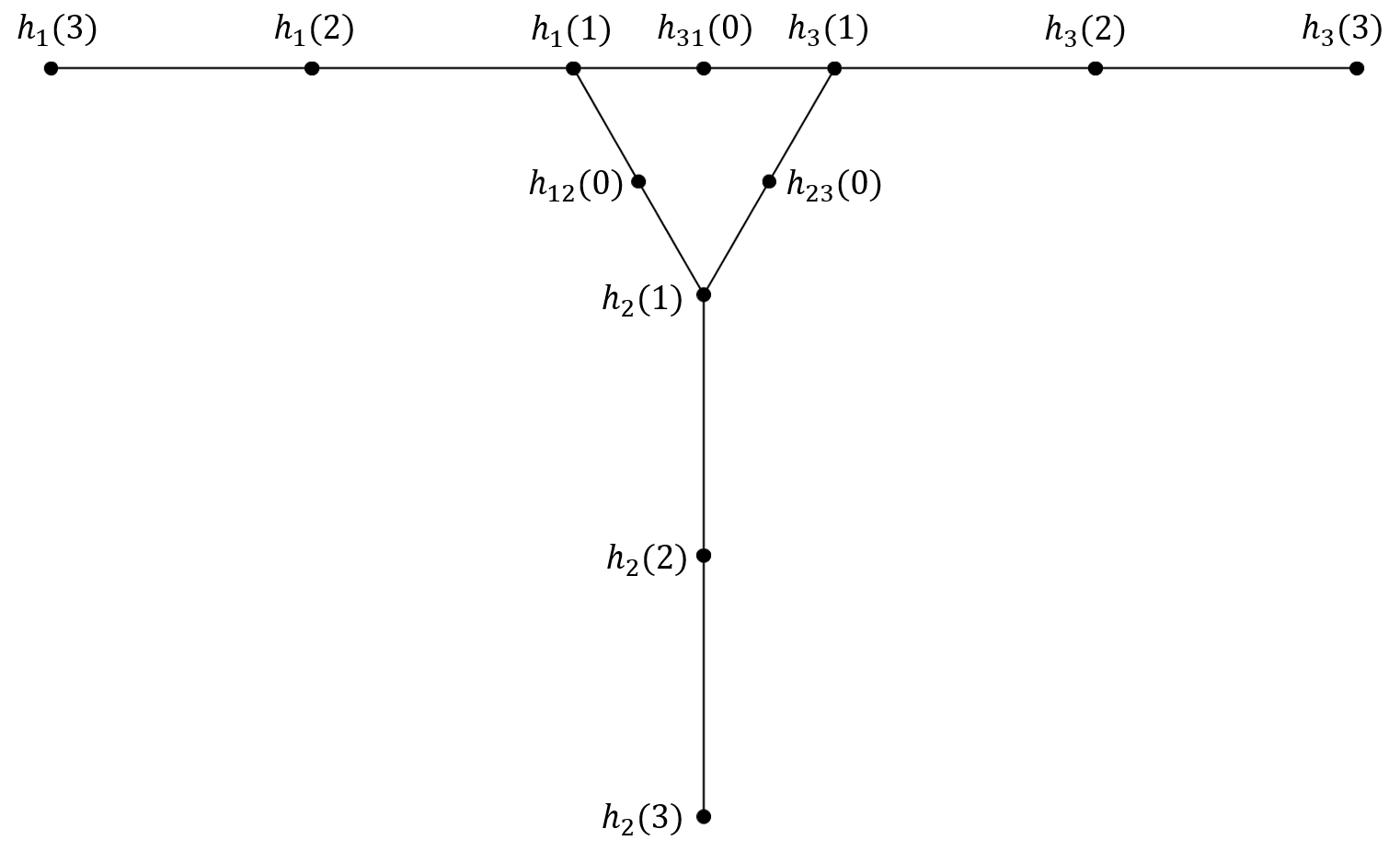
Figure 3: The CG of the tri-junction in Eq.(27). This CG is not an SPSC.

We find that the above requirement for $H^{\mathrm{junc}}$ is too general, allowing an infinite number of patterns of tri-junctions. To avoid the artificial complexity, we restrict the form of the junction as follows:

$$H^{\mathrm{junc}}=-\sum_{\mu=1}^{3}t_{\mu}h_{\mu}(1)-\sum_{\omega,\omega^{\prime}\in\Omega,\omega\neq\omega^{\prime}}g_{\omega,\omega^{\prime}}h_{\omega,\omega^{\prime}}(0),$$ (28)

where $\Omega$ is a set whose elements $\omega$ are subsets of $\{1,2,3\}$ and satisfy $\bigsqcup_{\omega\in\Omega}\omega=\{1,2,3\}$. More explicitly, $\Omega$ is one of the following sets

$$\{\{123\}\},\quad\{\{12\},\{3\}\},\quad\{\{1\},\{2\},\{3\}\},$$ (29)

and their permutations of the numbers. The first term in $H^{\mathrm{junc}}$ is the coupling to the spin chains, and the second term is the intra-junction coupling commuting with $H^{\mathrm{bulk}}$. We assume the simple coupling to the spin chains, $\{h_{\mu}(1),h_{\mu}(2)\}=0$, which satisfies the locality of the interaction and the connectivity in the resultant CG. This assumption also allows the mapping of the bulk spin chains to MQFs similar to Eq. (III.1):

$$H_{\mu}^{\mathrm{bulk}}=i\sum_{j=1}^{\infty} \left[J_{\mu}\varphi_{\mu}(2j-1)\varphi_{\mu}(2j)\right.$$

$$\left.+h_{\mu}\varphi_{\mu}(2j)\varphi_{\mu}(2j+1)\right].$$ (30)

For each $\Omega$, we specify the intra-junction coupling as follows: (i) $h_{\mu}(1)$ and $h_{\nu}(1)$ anti-commute with each other if there exists $\omega\in\Omega$ such that $\mu,\nu\in\omega$. (ii) $h_{\mu}(1)$ anti-commutes with $h_{\omega,\omega^{\prime}}(0)$ when $\mu\in\omega\cup\omega^{\prime}$. (iii) $h_{\omega,\omega^{\prime}}(0)$ and $h_{\omega^{\prime\prime},\omega^{\prime\prime\prime}}(0)$ anti-commutes with each other if they share a single subindex $\omega$. In other cases, we assume the commutation relations. The corresponding CGs show three patterns of SPSCs, as illustrated in Fig. 4.

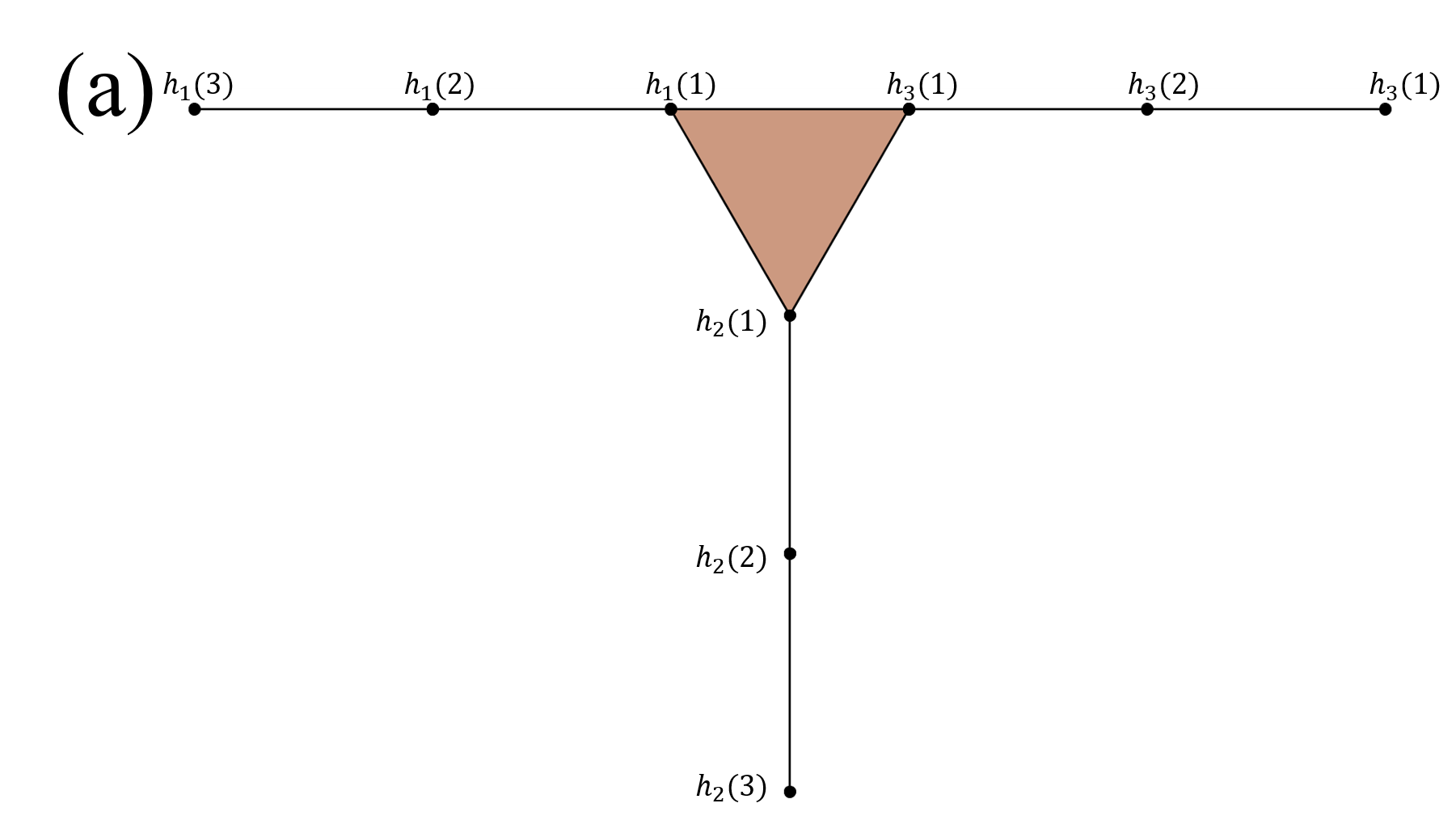
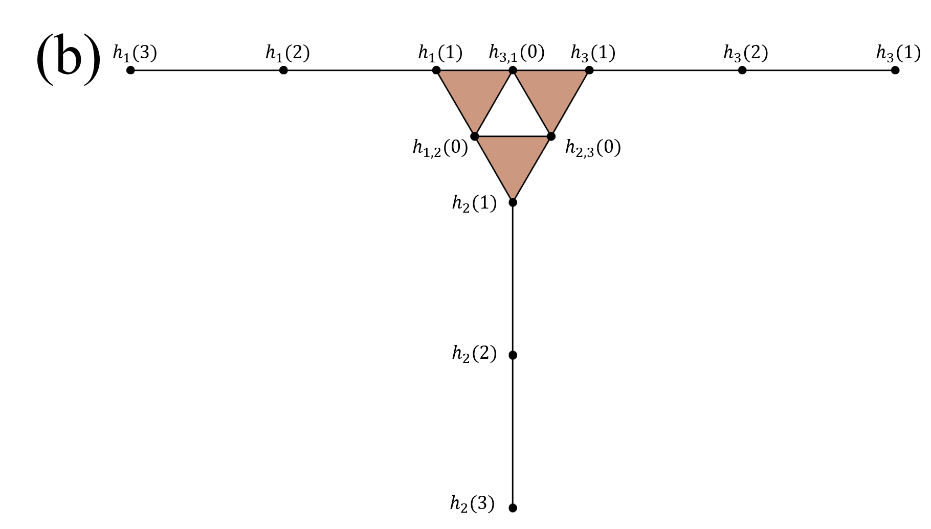
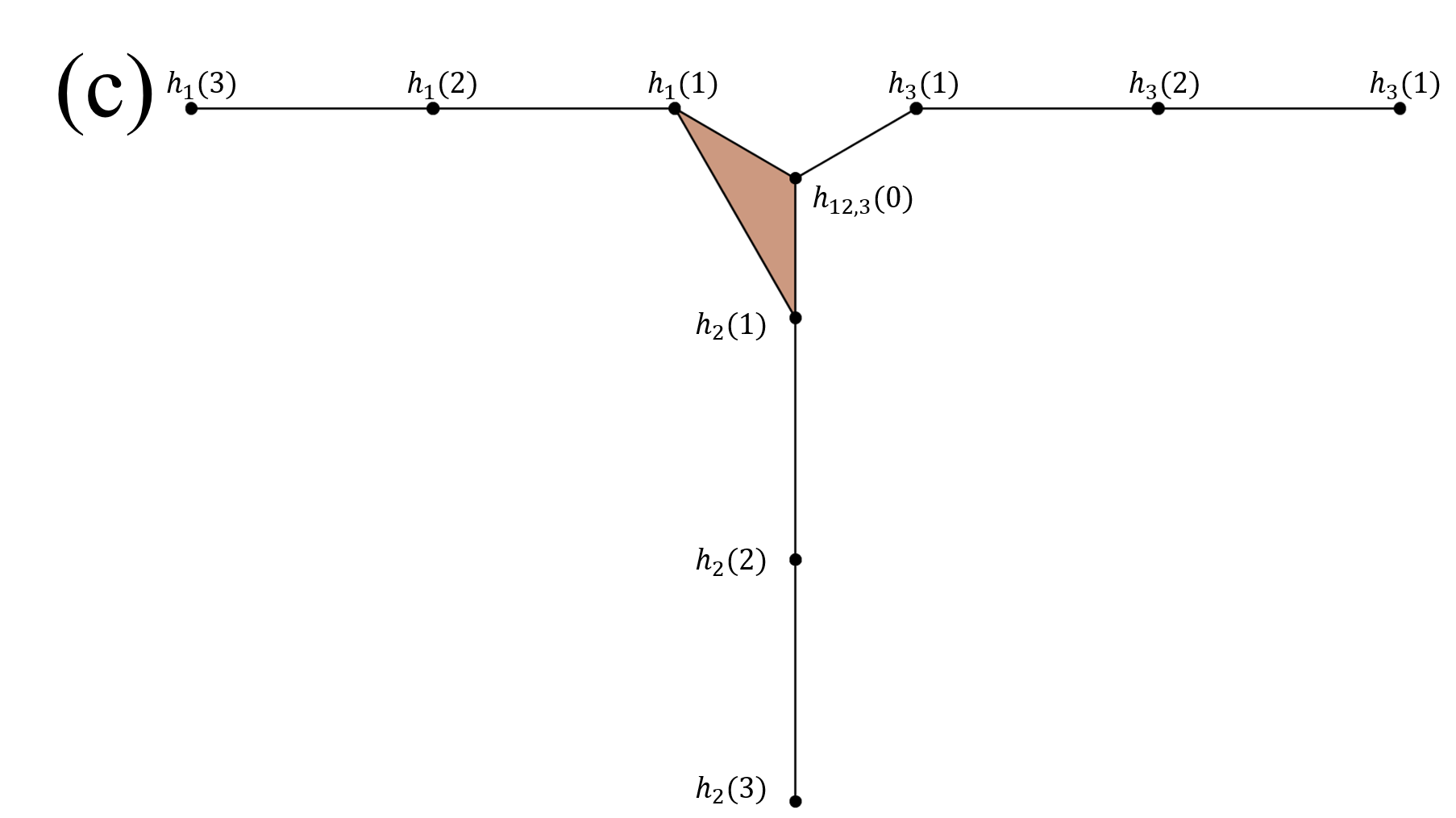
Figure 4: Three patterns of exactly solvable tri-junctions.(a) $(3)$-tri-junction. (b) $(1+1+1)$-tri-junction. (c) $(2+1)$-tri-junction.

These patterns can be understood as follows. Let $p(n)$ be the partition of a positive integer $n$, which is the number of possible divisions of $n$ into positive integers. Then, we have $p(3)=3$ as $3$ can be decomposed into positive integers in three different ways,

$$3 =3$$

$$=2+1$$

$$=1+1+1.$$ (31)

Because these divisions correspond to three patterns of tri-junctions, we call the tri-junctions in Fig 4 as $(3)$-, $(2+1)$-, and $(1+1+1)$-tri-junctions, respectively.

Similarly, we can easily obtain exactly solvable models for higher multi-junctions by using $H^{\mathrm{junc}}$ similar to Eq. (28). For example, because it holds $p(4)=5$,

$$4 =4$$

$$=3+1$$

$$=2+2$$

$$=2+1+1$$

$$=1+1+1+1,$$ (32)

we have five different patterns of exactly solvable tetra-junctions.

III.3 Majorana zero modes in tri-junctions

Here we examine various exactly solvable tri-junctions in Eq. (24). Since each bulk Hamiltonian $H_{\mu}^{\mathrm{bulk}}$ is essentially identical to Eq. (5), the bulk eigenequation for the spin chains is essentially the same as Eqs. (13) and (14),

$$-J_{\mu}w_{\mu}(n-1)+hw_{\mu}(n) =\lambda v_{\mu}(n),$$ (33)

$$-h_{\mu}v_{\mu}(n)+J_{\mu}v_{\mu}(n+1) =\lambda w_{\mu}(n),$$ (34)

with $n=1,2,\ldots$. Thus, in a manner similar to Sec.III.1, we can analyze the junctions by introducing the generating functions

$$V_{\mu}(z):=\sum_{n=1}^{\infty}v_{\mu}(n)z^{n},\quad W_{\mu}(z):=\sum_{n=1}^{\infty}w_{\mu}(n)z^{n},$$ (35)

The eigenequation for the junction part provides a boundary condition for the generating functions.

Table 1: The number of Majorana zero modes localized at the 1D $(3)$-, $(1+1+1)$-, and $(2+1)$-tri-junctions.

Conditions	$(3)$-tri-junction (I)	$(3)$-tri-junction (II)	$(1+1+1)$-tri-junction	$(2+1)$-tri-junction
$h_{1}<J_{1},h_{2}<J_{2},h_{3}<J_{3}$	1	2	1	0
$h_{1}>J_{1},h_{2}<J_{2},h_{3}<J_{3}$	0	1	0	1
$h_{1}<J_{1},h_{2}<J_{2},h_{3}>J_{3}$	0	1	0	1
$h_{1}>J_{1},h_{2}>J_{2},h_{3}<J_{3}$	1	0	1	2
$h_{1}>J_{1},h_{2}<J_{2},h_{3}>J_{3}$	1	0	1	0
$h_{1}>J_{1},h_{2}>J_{2},h_{3}>J_{3}$	2	1	0	1

III.3.1 $(3)$-Tri-Junction (I)

In the next two subsections, we analyse two different models for the $(3)$-tri-junction. First, in this subsection, we consider the following junction:

$$H^{\mathrm{junc}}= -t_{1}\sigma_{1}^{x}(1)\sigma_{2}^{z}(1)-t_{2}\sigma_{2}^{x}(1)\sigma_{3}^{z}(1)$$

$$-t_{3}\sigma_{3}^{x}(1)\sigma_{1}^{z}(3).$$ (36)

Defining $h_{\mu}(1)$ as

$$h_{1}(1)=\sigma_{1}^{x}(1)\sigma_{2}^{z}(1),\quad h_{2}(1)=\sigma_{2}^{x}(1)\sigma_{3}^{z}(1),$$

$$h_{3}(1)=\sigma_{3}^{x}(1)\sigma_{1}^{z}(1),$$ (37)

we have the CG in Fig. 4 (a). This CG is an SPSC by regarding each edge as a 1-simplex and the central triangle as a 2-simplex. As a result, we can map the Hamiltonian into a MQF:

$$H^{\mathrm{junc}}=i\sum_{\mu=1}^{3}t_{\mu}\varphi_{123}(0)\varphi_{\mu}(1),$$ (38)

where $\varphi_{123}(0)$ is a Majorana operator on the triangle. The corresponding eigenequation for the junction part is given by

$$\sum_{\mu=1}^{3}t_{\mu}w_{\mu}(0) =\lambda v_{123}(0),$$ (39)

$$-t_{\mu}v_{123}(0)+J_{\mu}v_{\mu}(1) =\lambda w_{\mu}(0)\quad(\mu=1,2,3).$$ (40)

From Eqs. (33), (34), and (40), the generating functions in Eq. (35) are determined as

$$V_{\mu}(z)= \frac{1}{h_{\mu}J_{\mu}}\frac{z}{z^{2}-2\kappa_{\mu}z+1}$$

$$\times\left[t_{\mu}\left(h_{\mu}-J_{\mu}z\right)v_{123}(0)+h_{\mu}\lambda w_{\mu}(0)\right],$$

$$W_{\mu}(z)= \frac{1}{h_{\mu}J_{\mu}}\frac{z}{z^{2}-2\kappa_{\mu}z+1}$$

$$\times\left[t_{\mu}\lambda v_{123}(0)-(J_{\mu}^{2}+\lambda^{2}-h_{\mu}J_{\mu}z)w_{\mu}(0)\right],$$ (41)

with

$$\kappa_{\mu}:=\frac{J_{\mu}^{2}+h_{\mu}^{2}+\lambda^{2}}{2J_{\mu}h_{\mu}}.$$ (42)

Now we focus on zero modes with $\lambda=0$. For zero modes, the generating functions read

$$V_{\mu}(z) =\frac{t_{\mu}}{h_{\mu}}v_{123}(0)\sum_{n=1}^{\infty}\left(\frac{h_{\mu}z}{J_{\mu}}\right)^{n},$$

$$W_{\mu}(z) =w_{\mu}(0)\sum_{n=1}^{\infty}\left(\frac{J_{\mu}z}{h_{\mu}}\right)^{n},$$ (43)

where $w_{\mu}(0)$ obeys Eq.(39) with $\lambda=0$,

$$\sum_{\mu=1}^{3}t_{\mu}w_{\mu}(0)=0.$$ (44)

To keep the $L^{2}$ condition of the corresponding eigenvectors, $v_{\mu}(n)$ and $w_{\mu}(n)$ must go to zero when $n\to\infty$. Thus, from Eq. (III.3.1), we have $w_{\mu}(0)=0$ ($v_{123}(0)=0$) if $h_{\mu}<J_{\mu}$ ($h_{\mu}>J_{\mu}$). Then, we have four different situations: (i) All the spin chains satisfy $h_{\mu}<J_{\mu}$. (ii) One of the spin chains, say the first one satisfies $h_{1}>J_{1}$, and the other chains satisfy $h_{2}<J_{2}$ and $h_{3}<J_{3}$. (iii) Two of the spin chains, say the first and the second ones satisfy $h_{1}>J_{1}$, and $h_{2}>J_{2}$, and the other satisfies $h_{3}<J_{3}$. (iv) All the spin chains satisfy $h_{\mu}>J_{\mu}$. For each of these cases, we can count the number of zero modes as follows.

For case (i), we have $w_{1}(0)=w_{2}(0)=w_{3}(0)$, which obeys Eq. (44). Thus, we have a single zero mode generated by $V_{\mu}(z)$ in Eq. (III.3.1) with $v_{123}(0)\neq 0$. For case (ii), we have $w_{2}(0)=w_{3}(0)$ and $v_{123}(0)=0$ from the $L^{2}$ condition. From Eq. (44), we also have $w_{3}(0)=0$. Hence $V_{\mu}(z)$ and $W_{\mu}(z)$ are identically zero, and thus no zero mode exists. For case (iii), the $L^{2}$ condition and Eq. (44) lead to $w_{3}(0)=v_{123}(0)=0$ and $t_{1}w_{1}(0)+t_{2}w_{2}(0)=0$. Thus, we have a single independent zero mode generated by $W_{1}(z)$ and $W_{2}(z)$ with $t_{1}w_{1}(0)+t_{2}w_{2}(0)=0$. Finally, for case (iv), a similar argument gives $v_{123}(0)=0$ and $t_{1}w_{1}(0)+t_{2}w_{2}(0)+t_{3}w_{3}(0)=0$, which lead to two independent zero modes generated by $W_{\mu=1,2,3}(z)$. All the obtained zero modes above are Majorana fermions localized at the junction. We summarize the number of Majorana junction modes in Table 1.

III.3.2 $(3)$-Tri-Junction (II)

Here we examine a different model for the $(3)$-tri-junction. The junction Hamiltonian is given by

$$H^{\mathrm{junc}}= -t_{1}\sigma_{1}^{x}(1)-t_{2}\sigma_{2}^{x}(1)-t_{3}\sigma_{3}^{x}(1)$$

$$-g_{1}\sigma_{1}^{z}(1)S^{x}-g_{2}\sigma_{2}^{z}(1)S^{y}-g_{3}\sigma_{3}^{z}(1)S^{z},$$ (45)

where $S^{a}$ $(a=x,y,z)$ is the Pauli matrix for an additional spin on the junction. Whereas the CG of this junction has the same form as Fig. 4(a), the properties of the junction are very different from those in Eq. (36) as we will show below.

Since this CG is an SPSC, the junction Hamiltonian can be rewritten in the form of MQFs by using the SPSC method,

$$H^{\mathrm{junc}}=i\sum_{\mu=1}^{3}\left[t_{\mu}\varphi_{\mu}(0)\varphi_{\mu}(1)+g_{\mu}\varphi_{123}(0)\varphi_{\mu}(0)\right],$$ (46)

where $\varphi_{\mu}(0)$ and $\varphi_{123}(0)$ are Majorana operators. The corresponding junction part of the eigenequation is

$$\sum_{\mu=1}^{3}g_{\mu}v_{\mu}(0) =\lambda v_{123}(0),$$

$$-g_{\mu}v_{123}(0)+t_{\mu}w_{\mu}(0) =\lambda v_{\mu}(0),$$

$$-t_{\mu}v_{\mu}(0)+J_{\mu}v_{\mu}(1) =\lambda w_{\mu}(0),$$ (47)

with $\mu=1,2,3$. Then, we find that the generating functions in Eq. (35) for zero modes with $\lambda=0$ become

$$V_{\mu}(z) =\frac{t_{\mu}}{h_{\mu}}v_{\mu}(0)\sum_{n=1}^{\infty}\left(\frac{h_{\mu}z}{J_{\mu}}\right)^{n},$$

$$W_{\mu}(z) =\frac{g_{\mu}}{t_{\mu}}v_{123}(0)\sum_{n=1}^{\infty}\left(\frac{J_{\mu}z}{h_{\mu}}\right)^{n},$$ (48)

with

$$\sum_{\mu=1}^{3}g_{\mu}v_{\mu}(0)=0.$$ (49)

In a manner similar to Sec. III.3.1, we can count the number of Majorana junction modes by demanding the $L^{2}$ condition. Note that the role of $V_{\mu}(z)$ and $W_{\mu}(z)$ is interchanged between Eqs.(III.3.1) and (III.3.2). Thus, the number of Majorana zero modes in the present junction does not coincide with that in the previous subsection. In particular, the parity of the Majorana mode number is opposite between these junctions. We summarize the obtained result in Table 1.

III.3.3 $(1+1+1)$-Tri-Junction

For a model of the $(1+1+1)$-tri-junction, we consider

$$H^{\mathrm{junc}}= -t_{1}\sigma_{1}^{x}(1)-t_{2}\sigma_{2}^{x}(1)-t_{3}\sigma_{3}^{x}(1)$$

$$-g_{12}\sigma_{1}^{z}(1)\sigma_{2}^{z}(1)S^{x}-g_{23}\sigma_{2}^{z}(1)\sigma_{3}^{z}(1)S^{y}$$

$$-g_{31}\sigma_{3}^{z}(1)\sigma_{1}^{z}(1)S^{z},$$ (50)

where $S^{a}$ is the Pauli matrix for an additional spin. The CG of this Hamiltonian is an SPSC in Fig. 4 (b). The Hamiltonian in an MQF is

$$H^{\mathrm{junc}}= i\sum_{\mu=1}^{3}t_{\mu}\varphi_{\mu}(0)\varphi_{\mu}(1)+ig_{12}\epsilon_{12}\varphi_{1}(0)\varphi_{2}(0)$$

$$+ig_{23}\epsilon_{23}\varphi_{2}(0)\varphi_{3}(0)+ig_{31}\epsilon_{31}\varphi_{3}(0)\varphi_{1}(0),$$ (51)

with $\epsilon_{\mu\nu}=\pm 1$. Here using the $\mathbb{Z}_{2}$ gauge transformation, we have set $\epsilon_{12}=\epsilon_{23}=1$. The remaining sign $\epsilon_{13}$ is determined by the conserved quantity of the hole in Fig. 4 (b). In the present case, the conserved quantity is $i$, which implies $\epsilon_{31}=1$.

The eigenequation for the junction is

$$t_{1}w_{1}(0)+g_{12}v_{2}(0)-g_{31}v_{3}(0) =\lambda v_{1}(0),$$

$$-g_{12}v_{1}(0)+t_{2}w_{2}(0)+g_{23}v_{3}(0) =\lambda v_{2}(0),$$

$$g_{31}v_{1}(0)-g_{23}v_{2}(0)+t_{3}w_{3}(0) =\lambda v_{3}(0),$$

$$-t_{\mu}v_{\mu}(0)+J_{\mu}v_{\mu}(1) =\lambda w_{\mu}(0),$$ (52)

with $\mu=1,2,3$. Equations. (33) and (34) still work as the bulk eigenequation for the spin chains, and hence we have the bulk generating functions in the form of Eq. (III.3.1) with replacing $v_{123}(0)$ by $v_{\mu}(0)$.

For zero modes with $\lambda=0$, we have Eq. (III.3.1) with replacing $v_{123}(0)$ by $v_{\mu}(0)$. We also have the constraint at the junction

$$t_{1}w_{1}(0)+g_{12}v_{2}(0)-g_{31}v_{3}(0) =0,$$

$$-g_{12}v_{1}(0)+t_{2}w_{2}(0)+g_{23}v_{3}(0) =0,$$

$$g_{31}v_{1}(0)-g_{23}v_{2}(0)+t_{3}w_{3}(0) =0.$$ (53)

Considering the $L^{2}$ condition, we can count Majorana junction modes. The result is summarized in Table 1.

III.3.4 $(2+1)$-Tri-Junction

An example of the $(2+1)$-tri-junction is

$$H^{\mathrm{junc}}= -t_{1}\sigma_{1}^{x}(1)-t_{2}\sigma_{2}^{x}(1)\sigma_{1}^{z}(1)-t_{3}\sigma_{3}^{x}(1)$$

$$-g_{12,3}\sigma_{1}^{z}(1)\sigma_{2}^{z}(1)\sigma_{3}^{z}(1).$$ (54)

The CG of this model is Fig. 4(c), which is an SPSC. The junction Hamiltonian in the form of an MQF is,

$$H^{\mathrm{junc}}= it_{1}\varphi_{12}(0)\varphi_{1}(1)+it_{2}\varphi_{12}(0)\varphi_{2}(1)$$

$$+it_{3}\varphi_{3}(0)\varphi_{3}(1)+ig_{12,3}\varphi_{12}(0)\varphi_{3}(0).$$ (55)

Hence the eigenequation for the junction becomes

$$t_{1}w_{1}(0)+t_{2}w_{2}(0)+g_{12,3}v_{3}(0) =\lambda v_{12}(0),$$

$$-g_{12,3}v_{12}(0)+t_{3}w_{3}(0) =\lambda v_{3}(0),$$

$$-t_{\mu}v_{\mu}(0)+J_{\mu}v_{\mu}(1) =\lambda w_{\mu}(0),$$ (56)

with $\mu=1,2,3$. For zero modes with $\lambda=0$, we have again Eq. (III.3.1) with replacing $v_{123}(0)$ by $v_{12}(0)$ ($v_{3}(0)$) in $V_{\mu=1,2}(z)$ ($V_{3}(z)$). We also have the boundary condition at the junction,

$$t_{1}w_{1}(0)+t_{2}w_{2}(0)+g_{12,3}v_{3}(0) =0,$$

$$-g_{12,3}v_{12}(0)+t_{3}w_{3}(0) =0.$$ (57)

In a manner similar to other junctions, we can count Majorana junction modes. The result is summarized in Table 1.

IV Tri-Junctions of 2D spin lattices

In this section, we construct exactly solvable tri-junctions of two-dimensional (2D) spin lattices and examine their properties.

IV.1 2D spin lattice

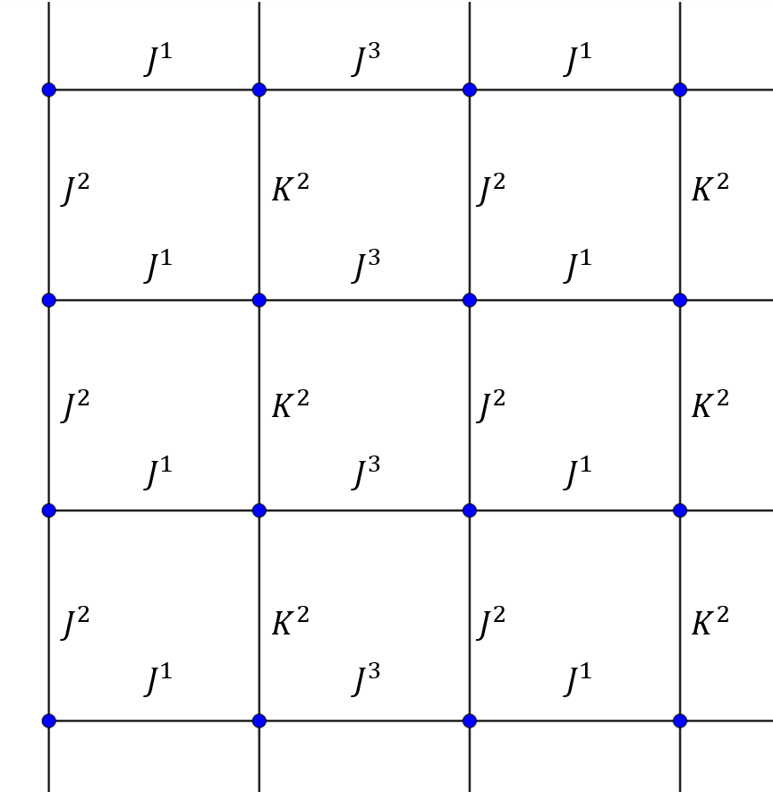
Figure 5: Half-plane square lattice. A $SO(5)$-spin is placed on each vertex. Labels on edges represent the exchange constants of spins.

As a 2D spin lattice system, we consider an $SO(5)$-spin model on the square lattice. We put the $SO(5)$ Dirac matrices

$$\alpha^{a}(m,n) =\sigma^{a}(m,n)\otimes\tau^{x}(m,n)\quad(a=1,2,3),$$

$$\alpha^{4}(m,n) =\sigma^{0}(m,n)\otimes\tau^{z}(m,n),$$

$$\alpha^{5}(m,n) =\sigma^{0}(m,n)\otimes\tau^{y}(m,n),$$ (58)

on each vertex of the half-plane square lattice in Fig. 5, and introduce the Hamiltonian as

$$H=-\sum_{m=1}^{\infty}\sum_{n\in\mathbb{Z}}[ J^{1}h^{1}(2m-1,n)+J^{3}h^{1}(2m,n)$$

$$+J^{2}h^{2}(2m-1,n)+K^{2}h^{2}(2m,n)$$

$$+J^{5}h^{\prime}(m,n)],$$

$$-t\sum_{n\in\mathbb{Z}} h^{3}(1,n),$$ (59)

where

$$h^{1}(2m-1,n) =\alpha^{1}(2m-1,n)\alpha^{1}(2m,n),$$

$$h^{1}(2m,n) =\alpha^{3}(2m,n)\alpha^{3}(2m+1,n),$$

$$h^{2}(2m-1,n) =\alpha^{2}(2m-1,n)\alpha^{4}(2m-1,n+1),$$

$$h^{2}(2m,n) =\alpha^{2}(2m,n)\alpha^{4}(2m,n+1),$$

$$h^{\prime}(m,n) =\alpha^{5}(m,n),\quad h^{3}(1,n)=\alpha^{3}(1,n).$$ (60)

The CG of this Hamiltonian is given by Fig. 6.

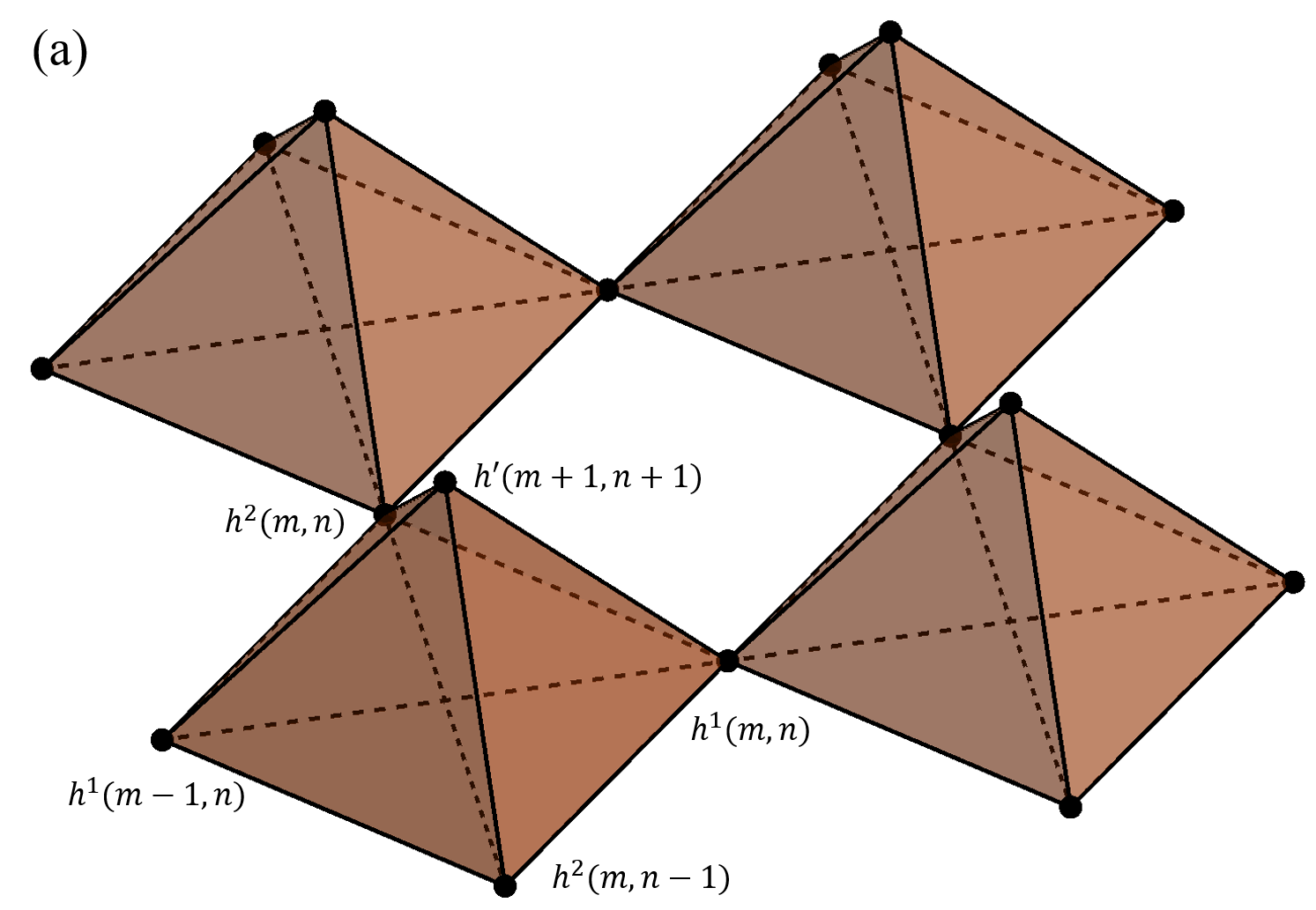
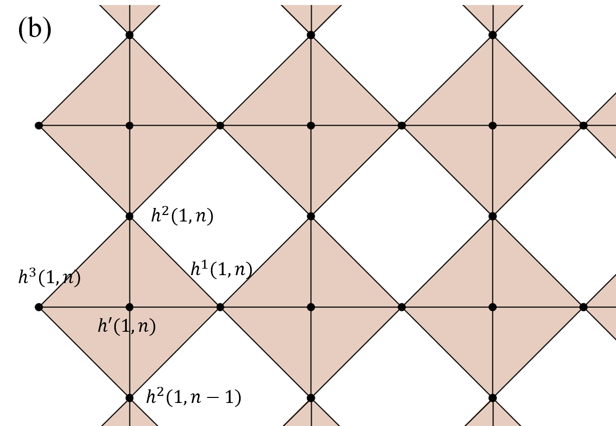
Figure 6: The CG of the $SO(5)$-spin square lattice. The right figure (b) is a simplified version of the left one (a), which we use in Fig.8.

Regarding each square pyramid and each endpoint in Fig. 6 as a 4-simplex and a 0-simplex, respectively, we can identify the CG as an SPSC. Thus, each term of the Hamiltonian is equivalent to an MQF:

$$h^{1}(m,n) =-i\epsilon^{1}(m,n)\varphi(m,n)\varphi(m+1,n),$$

$$h^{2}(m,n) =-i\epsilon^{2}(m,n)\varphi(m,n)\varphi(m+1,n),$$

$$h^{\prime}(m,n) =-i\epsilon^{\prime}(m,n)\varphi(m,n)\varphi^{\prime}(m,n),$$

$$h^{3}(1,n) =-i\epsilon^{3}(1,n)\varphi(0,n)\varphi(1,n),$$ (61)

where $\epsilon^{d}(m,n)$’s and $\epsilon^{\prime}(m,n)$’s are sign factors. Using the gauge transformation, we can set

$$\epsilon^{1}(m,n)=\epsilon^{2}(1,n)=\epsilon^{3}(1,n)=\epsilon^{\prime}(m,n)=1$$ (62)

for any $m=,1,2,\ldots$ and $n\in\mathbb{Z}$. The remaining factors are given by the conserved quantities on the holes in Fig. 6. Namely, we have the conserved quantity $c(m,n)$

$$c(m,n):= h^{2}(m,n)h^{1}(m,n+1)h^{2}(m+1,n)h^{1}(m,n)$$

$$= \epsilon^{2}(m,n)\epsilon^{2}(m+1,n),$$ (63)

which determine the remaining factors. From the Lieb’s theorem Lieb (2004); Macris and Nachtergaele (1996), we have $c(m,n)=-1$ for the ground state of this model, which fixes the remaining factors as

$$\epsilon^{2}(m,n)=(-1)^{m+1}.$$ (64)

Hereafter we set $J^{5}=0$ for simplicity.

Since our model has lattice translation symmetry in the $n$-direction, it is convenient to perform the Fourier transformation in the $n$-direction:

$$\varphi(m,n)=\frac{1}{\sqrt{\pi}}\int_{-\pi}^{\pi}dk_{y}a(m,k_{y})e^{-ik_{y}n}\quad(m=0,1,2,\ldots),$$ (65)

where $k_{y}$ is the momentum in the $n$-direction, and $a(m,k_{y})$ satisfies

$$a(m,k_{y})^{\dagger} =a(m,-k_{y}),$$

$$\{a(m,k_{y}),a(m^{\prime},k_{y}^{\prime})^{\dagger}\} =\delta_{m,m^{\prime}}\delta(k_{y}-k_{y}^{\prime}).$$ (66)

After the Fourier transformation, we get

$$H=\int_{-\pi}^{\pi}dk_{y}\vec{a}(k_{y})^{\dagger}\mathcal{H}(k_{y})\vec{a}(k_{y}),$$ (67)

where

$$\vec{a}(k_{y})=\begin{pmatrix}a(0,k_{y})&a(1,k_{y})&a(2,k_{y})&\cdots\end{pmatrix}^{T}$$ (68)

and

$$\mathcal{H}(k_{y})=$$

$$\begin{pmatrix}0&it\\ -it&2J^{2}\sin k_{y}&iJ^{1}&\\ &-iJ^{1}&-2K^{2}\sin k_{y}&iJ^{3}&\\ &&-iJ^{3}&2J^{2}\sin k_{y}&iJ^{1}\\ &&&-iJ^{1}&\ddots&\ddots\\ &&&&\ddots\end{pmatrix}.$$ (69)

We solve the energy eigenequation of $\mathcal{H}(k_{y})$. Let $E(k_{y})$ be an eigenenergy of $\mathcal{H}(k_{y})$ with an eigenvector

$$\vec{v}(k_{y})=\begin{pmatrix}v(0,k_{y})&w(0,k_{y})&v(1,k_{y})&w(1,k_{y})&\cdots\end{pmatrix}^{T}.$$ (70)

Then, the eigenequation gives

$$itw(0,k_{y})=Ev(0,k_{y}),$$ (71)

$$-itv(0,k_{y})+2J^{2}\sin k_{y}w(0,k_{y})$$

$$\quad+iJ^{1}v(1,k_{y})=Ew(0,k_{y}),$$ (72)

$$-iJ^{1}w(n-1,k_{y})-2K^{2}\sin k_{y}v(n,k_{y})$$

$$\quad+iJ^{3}w(n,k_{y})=Ev(n,k_{y}),$$ (73)

$$-iJ^{3}v(n,k_{y})+2J^{2}\sin k_{y}w(n,k_{y})$$

$$\quad+iJ^{1}v(n+1,k_{y})=Ew(n,k_{y}),$$ (74)

with $n=1,2,\ldots$. To solve the eigenequation, we introduce the generating functions,

$$V(z)=\sum_{n=1}^{\infty}z^{n}v(n,k_{y}),\quad W(z)=\sum_{n=1}^{\infty}z^{n}w(n,k_{y}).$$ (75)

Then, from Eqs. (72), (73) and (74), we get

$$\begin{pmatrix}E+2K^{2}\sin k_{y}&i(J^{1}z-J^{3})\\ i(J^{3}-iJ^{1}z^{-1}&E-2J^{2}\sin k_{y}\end{pmatrix}\begin{pmatrix}V\\ W\end{pmatrix}$$

$$=-w(0)\begin{pmatrix}iJ^{1}z\\ E-2J^{2}\sin k_{y}\end{pmatrix}-v(0)\begin{pmatrix}0\\ it\end{pmatrix}.$$ (76)

Hence we obtain

$$V(z) =\frac{-z}{J^{1}J^{3}(z^{2}-2\kappa z+1)}$$

$$\times\left[t(J^{1}z-J^{3})v(0,k_{y})\right.$$

$$\left.\quad+iJ^{3}(E-2J^{2}\sin k_{y})w(0,k_{y})\right],$$

$$W(z) =\frac{-z}{J^{1}J^{3}(z^{2}-2\kappa z+1)}$$

$$\times\left[it(E+2K^{2}\sin k_{y})v(0,k_{y})\right.$$

$$\left.\quad+(J^{3}-2J^{1}\kappa+J^{1}z)w(0,k_{y})\right],$$ (77)

where

$$\kappa:=\frac{1}{2J^{1}J^{3}}[ (J^{1})^{2}+(J^{3})^{2}$$

$$-(E-2J^{2}\sin k_{y})(E+2K^{2}\sin k_{y})].$$ (78)

We can obtain the bulk spectrum as follows. Let $z_{\pm}$ be the roots of $z^{2}-2\kappa z+1$. Then, in a manner similar to the transverse field Ising model, the bulk spectrum requires $|z_{\pm}|=1$, i.e. $z_{\pm}=e^{\pm ik_{x}}$ ($k_{y}\in(-\pi,\pi]$), which leads to

$$E=(J^{2}-K^{2})\sin k_{y}\pm \left[\{(J^{2}+K^{2})\sin k_{y}\}^{2}\right.$$

$$\left.+(J^{1})^{2}+(J^{3})^{2}-2J^{1}J^{3}\sin k_{x}\right].$$ (79)

For boundary zero modes with $E=0$, the generating functions become

$$V(z)= \frac{-z}{J^{1}J^{3}(z^{2}-2\kappa z+1)}$$

$$\times\left[t(J^{1}z-J^{3})v(0)-2iJ^{3}J^{2}\sin k_{y}w(0,k_{y})\right],$$

$$W(z)= \frac{-z}{J^{1}J^{3}(z^{2}-2\kappa z+1)}$$

$$\times\left[2itK^{2}\sin k_{y}v(0)\right.$$

$$\left.\quad+(J^{3}-2J^{1}\kappa+J^{1}z)w(0,k_{y})\right].$$ (80)

The terms involving $\sin k_{y}$ in Eq. (IV.1) requires $k_{y}=0,\pi$ to satisfy $|z_{\pm}|\neq 1$. Under this condition, we get

$$V(z) =\frac{tz}{J^{1}-J^{3}z}v(0,k_{0})=\frac{t}{J^{1}}v(0)\sum_{n=1}^{\infty}\left(\frac{J^{3}z}{J^{1}}\right)^{n},$$

$$W(z) =\frac{J^{1}z}{J^{3}-J^{1}z}w(0,k_{0})=w(0)\sum_{n=1}^{\infty}\left(\frac{J^{1}z}{J^{3}}\right)^{n},$$ (81)

with $k_{0}=0,\pi$. Moreover, Eq. (71) leads to $w(0,k_{0})=0$, which means $W(z)=0$. Then, from the $L^{2}$ condition for $v(n,k_{0})$ of $V(z)$, we find that a zero energy edge state exists at $k_{y}=0,\pi$ when $J^{1}>J^{3}$. In Fig. 7 (a), we show the spectrum of the system under the open boundary condition in the $m$-direction, which confirms the existence of the edge states for $J^{1}>J^{3}$.

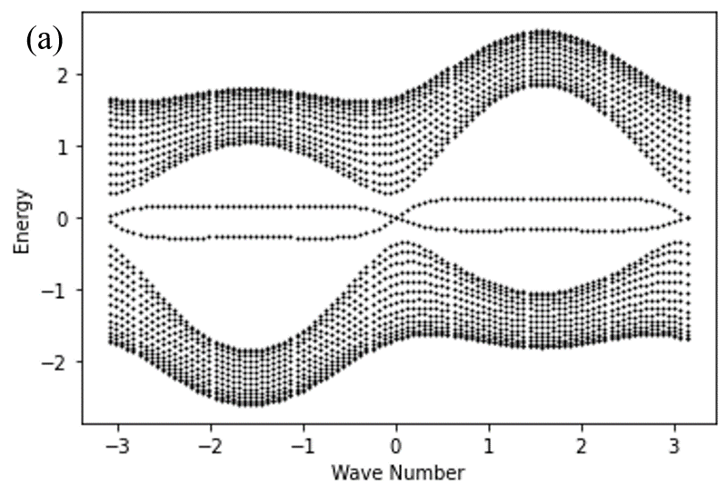
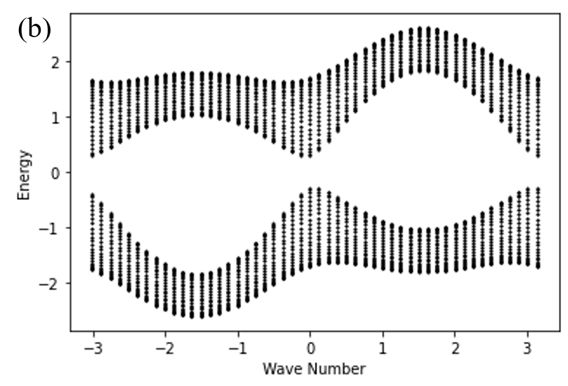
Figure 7: The energy spectra of the $SO(5)$-spin lattice under (a) the open boundary condition (OBC) and (b) the periodic boundary condition (PBC) in the $m$-direction. The horizontal axis is the wave number $k_{y}$ in the $n$-direction. Here we take the model parameters as $J^{1}=1,J^{2}=0.9,J^{3}=0.7,K^{2}=0.5$, and $t=0.7$. Majorana modes along the tri-junction appear under the OBC.

Note that if we replace $J^{1}$ and $J^{3}$ with $J$ and $h$ respectively and set $k_{y}=0,\pi$ (or $J^{2}=K^{2}=0$), $\mathcal{H}$ coincides with the Hamiltonian of the transverse field Ising model in Eq. (III.1).

IV.2 Exactly Solvable Tri-Junctions of 2D Spins

This section gives a class of exactly solvable tri-junctions of a 2D spin system by generalizing the arguments in Sec. III.2. The model we consider is

$$H=H^{\mathrm{junc}}+\sum_{\mu=1}^{3}H_{\mu}^{\mathrm{bulk}}.$$ (82)

Here $H^{\mathrm{bulk}}_{\mu}$ is the 2D $SO(5)$-spin lattice Hamiltonian, which is given by

$$H_{\mu}^{\mathrm{bulk}}=-\sum_{m=1}^{\infty}\sum_{n\in\mathbb{Z}}[ J_{\mu}^{1}h^{1}_{\mu}(2m-1,n)+J_{\mu}^{3}h_{\mu}^{1}(2m,n)$$

$$+J_{\mu}^{2}h_{\mu}^{2}(2m-1,n)+K_{\mu}^{2}h_{\mu}^{2}(2m,n)],$$ (83)

where

$$h_{\mu}^{1}(2m-1,n) =\alpha_{\mu}^{1}(2m-1,n)\alpha_{\mu}^{1}(2m,n),$$

$$h_{\mu}^{1}(2m,n) =\alpha_{\mu}^{3}(2m,n)\alpha_{\mu}^{3}(2m+1,n),$$

$$h_{\mu}^{2}(2m-1,n) =\alpha_{\mu}^{2}(2m-1,n)\alpha_{\mu}^{4}(2m-1,n+1),$$

$$h_{\mu}^{2}(2m,n) =\alpha_{\mu}^{2}(2m,n)\alpha_{\mu}^{4}(2m,n+1),$$ (84)

and the $SO(5)$ Dirac matrices are defined by

$$\alpha_{\mu}^{a}(m,n) =\sigma_{\mu}^{a}(m,n)\otimes\tau_{\mu}^{x}(m,n),\quad(a=1,2,3)$$

$$\alpha_{\mu}^{4}(m,n) =\sigma_{\mu}^{0}(m,n)\otimes\tau_{\mu}^{z}(m,n),$$

$$\alpha_{\mu}^{5}(m,n) =\sigma_{\mu}^{0}(m,n)\otimes\tau_{\mu}^{y}(m,n).$$ (85)

$H^{\mathrm{junc}}$ is the junction Hamiltonian determined below.

Like tri-junctions of spin chains, we determine $H^{\mathrm{junc}}$ as follows. Let $\Omega$ be a set whose elements $w$ are subsets of $\{1,2,3\}$ and satisfy $\bigsqcup_{\omega\in\Omega}\omega=\{1,2,3\}$. (See Eq. (29).) Then, we consider the junction in the form of

$$H^{\mathrm{junc}}= -t\sum_{\mu=1}^{3}\sum_{n\in\mathbb{Z}}h_{\mu}^{3}(1,n)$$

$$-\sum_{n\in\mathbb{Z}}\sum_{\omega,\omega^{\prime}\in\Omega,\omega\neq\omega^{\prime}}g_{\omega,\omega^{\prime}}h_{\omega,\omega^{\prime}}(n),$$ (86)

where the first term is the coupling to the 2D lattices, and the second is the intra-junction coupling that commutes with $H^{\mathrm{bulk}}$. We require that $h_{\mu}^{3}(1,n)$ and $h_{\omega,\omega^{\prime}}(n)$ satisfy the same anti-commuatation relation as those of $h_{\mu}(1)$ and $h_{\omega,\omega^{\prime}}(0)$ in Eq. (28) for each $n$, and all the other relations are commutative.

The resultant junction is exactly solvable. In Fig. 8, we show CGs of $H$ satisfying the condition above. Corresponding to three different $\Omega$ in Eq. (29), we obtain three different patterns of CGs, all of which are SPSCs.

In this method, we have the same MQF of $H_{\mu}^{\mathrm{bulk}}$ as Eq. (IV.1):

$$h_{\mu}^{1}(m,n) =-i\varphi_{\mu}(m,n)\varphi_{\mu}(m+1,n),$$

$$h_{\mu}^{2}(m,n) =-i(-1)^{m+1}\varphi_{\mu}(m,n)\varphi_{\mu}(m+1,n),$$ (87)

where we fix the sign factors using the Lieb’s theorem. As a result, we have the same eigenequation for each of the 2D spin lattices,

$$-iJ_{\mu}^{1}w_{\mu}(n-1,k_{y})-2K_{\mu}^{2}\sin k_{y}v_{\mu}(n,k_{y})$$

$$\quad+iJ_{\mu}^{3}w_{\mu}(n,k_{y})=Ev_{\mu}(n,k_{y}),$$

$$-iJ_{\mu}^{3}v_{\mu}(n,k_{y})+2J_{\mu}^{2}\sin k_{y}w_{\mu}(n,k_{y})$$

$$\quad+iJ_{\mu}^{1}v_{\mu}(n+1,k_{y})=Ew_{\mu}(n,k_{y}),$$ (88)

with $n=1,2,\ldots$. Thus we can solve the obtained junctions by using the generating functions in a manner similar to Sec. IV.1.

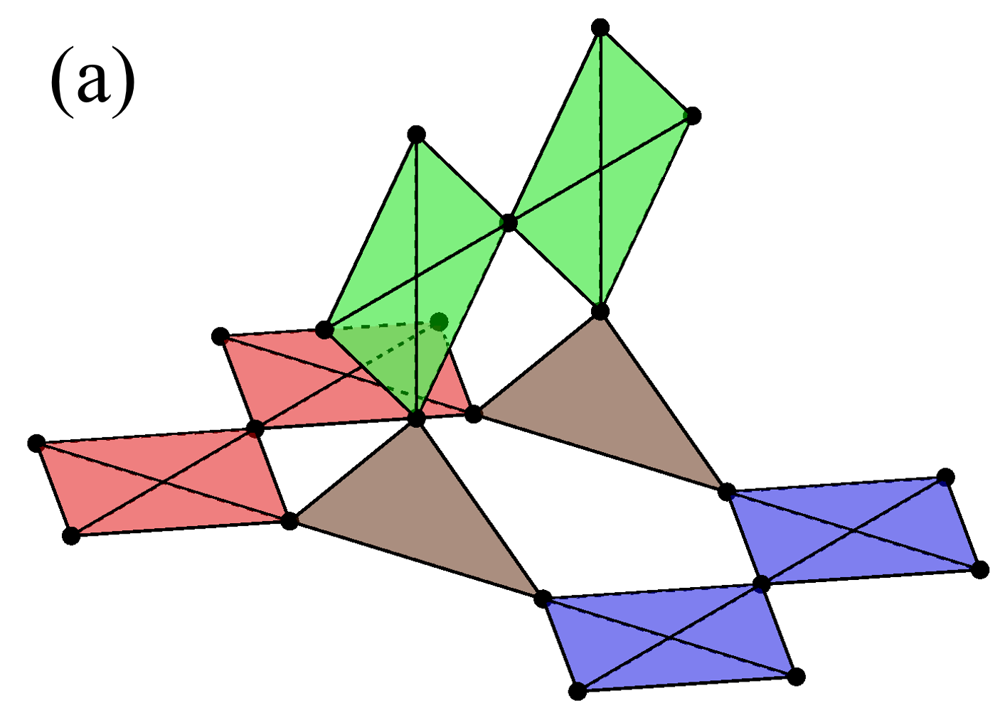
Figure 8: Three patterns of tri-junctions of 2D $SO(5)$-spin lattices. (a) (3)-tri-junction. (b) (1+1+1)-tri-junction. (c) (2+1)-tri-junction.

IV.3 Majorana junction states

Table 2: The number of Majorana modes along the 2D $(3)$-, $(1+1+1)$-, and $(2+1)$-tri-junctions of the 2D $SO(5)$ spin lattices.

Conditions	$(3)$-tri-junction	$(1+1+1)$-tri-junction	$(2+1)$-tri-junction
$J^{3}_{1}<J^{1}_{1},J^{3}_{2}<J^{1}_{2},J^{3}_{3}<J^{1}_{3}$	1	1	0
$J^{3}_{1}>J^{1}_{1},J^{3}_{2}<J^{1}_{2},J^{3}_{3}<J^{1}_{3}$	0	0	1
$J^{3}_{1}<J^{1}_{1},J^{3}_{2}<J^{1}_{2},J^{3}_{3}>J^{1}_{3}$	0	0	1
$J^{3}_{1}>J^{1}_{1},J^{3}_{2}>J^{1}_{2},J^{3}_{3}<J^{1}_{3}$	1	1	2
$J^{3}_{1}>J^{1}_{1},J^{3}_{2}<J^{1}_{2},J^{3}_{3}>J^{1}_{3}$	1	1	0
$J^{3}_{1}>J^{1}_{1},J^{3}_{2}>J^{1}_{2},J^{3}_{3}>J^{1}_{3}$	2	0	1

IV.3.1 $(3)$-Tri-Junction

First, we consider the $(3)$-tri-junction in Fig. 8(a) i.e., the tri-junction with $\Omega=\{123\}$. To realize this junction, we consider

$$h_{\mu}^{3}(1,n)=\alpha_{\mu}^{3}(1,n)\zeta_{\mu+1}^{3}(1,n),\quad h_{\omega,\omega^{\prime}}(n)=0$$ (89)

in Eq.(86), where

$$\zeta_{\mu}^{3}(1,n)=-\sigma_{\mu}^{3}(1,n)\otimes\tau_{\mu}^{z}(1,n)$$ (90)

with $\zeta_{4}^{3}(1,n)=\zeta_{1}^{3}(1,n)$. In an MQF, we have

$$h_{\mu}^{3}(1,n)=-i\epsilon_{\mu}(n)\varphi_{123}(0,n)\varphi_{\mu}(1,n),$$ (91)

where $\epsilon_{\mu}(n)$ is a sign factor, which we set $\epsilon_{\mu}(n)=1$ using the Leib’s theorem. After the Fourier transformation, the junction Hamiltonian is recast into

$$H^{\mathrm{junc}}=\sum_{\mu=1}^{3}it_{\mu}\int_{-\pi}^{\pi}dk_{y}a_{123}(0,k_{y})^{\dagger}a_{\mu}(1,k_{y})+\mathrm{h.c.}.$$ (92)

Thus, the eigenequation for the junction part is

$$\sum_{\mu=1}^{3}it_{\mu}w_{\mu}(0,k_{y})=Ev_{123}(0,k_{y}),$$

$$-it_{\mu}v_{123}(0,k_{y})+2J_{\mu}^{2}\sin k_{y}w_{\mu}(0,k_{y})+iJ_{\mu}^{1}v_{\mu}(1,k_{y})$$

$$\quad=Ew_{\mu}(0,k_{y}),$$ (93)

with $\mu=1,2,3$. From this equation and Eq. (88), the generating functions

$$V_{\mu}(z)=\sum_{n=1}^{\infty}v_{\mu}(n,k_{y})z^{n},\quad W_{\mu}(z)=\sum_{n=1}^{\infty}w_{\mu}(n,k_{y})z^{n}$$ (94)

are calculated as

$$V_{\mu}(z)= \frac{-z}{J_{\mu}^{3}(z^{2}-2\kappa_{\mu}z+1)}$$

$$\times\left[t_{\mu}(J_{\mu}^{1}z-J_{\mu}^{3})v_{\mu}(0,k_{y})\right.$$

$$\left.\quad+iJ_{\mu}^{3}(E-2J_{\mu}^{2}\sin k_{y})w(0,k_{y})\right],$$

$$W_{\mu}(z)= \frac{-z}{J_{\mu}^{1}(z^{2}-2\kappa_{\mu}z+1)}$$

$$\times\left[it_{\mu}(E+2K_{\mu}^{2}\sin k_{y})v(0,k_{y})\right.$$

$$\left.\quad+(J_{\mu}^{3}-2J_{\mu}^{1}\kappa_{\mu}+J_{\mu}^{1}z)w(0,k_{y})\right],$$ (95)

where

$$\kappa_{\mu}:=\frac{1}{2J_{\mu}^{1}J_{\mu}^{3}} \left[(J_{\mu}^{1})^{2}+(J_{\mu}^{3})^{2}\right.$$

$$\left.-(E-2J_{\mu}^{2}\sin k_{y})(E+2K_{\mu}^{2}\sin k_{y})\right].$$ (96)

To consider Majorana junction modes, we set $E=0$ and $k_{y}=0,\pi$. Under this condition, the generating functions read

$$V_{\mu}(z) =\frac{t_{\mu}}{J_{\mu}^{1}}v_{123}(0,k_{0})\sum_{n=1}^{\infty}\left(\frac{J_{\mu}^{3}z}{J_{\mu}^{1}}\right)^{n},$$

$$W_{\mu}(z) =w_{\mu}(0,k_{0})\sum_{n=1}^{\infty}\left(\frac{J_{\mu}^{1}z}{J_{\mu}^{3}}\right)^{n}\quad(k_{0}=0,\pi),$$ (97)

which coincide with $V_{\mu}(z)$ and $W_{\mu}(z)$ in Eq.(III.3.1) with $J_{\mu}=J_{\mu}^{1}$ and $h_{\mu}=J_{\mu}^{3}$. Moreover, for $E=0$ and $k_{y}=0,\pi$, Eq. (93) leads to the same constraint as Eq. (44). Thus, we can count the number of Majorna junction modes similarly. We summarize the result in Table 2.

IV.3.2 $(1+1+1)$-Tri-Junction

An example of the $(1+1+1)$-tri-junction in Fig. 8 (b), i.e., the tri-junction with $\Omega=\{\{1\},\{2\},\{3\}\}$, we consider

$$h_{\mu}^{3}(1,n)=\alpha^{3}_{\mu}(1,n),\quad h_{\mu,\nu}(n)=\zeta_{\mu}^{3}(1,n)S^{\rho}(n)\zeta_{\nu}^{3}(1,n),$$ (98)

where we take $\omega=\mu$ and $\omega^{\prime}=\nu$ in $h_{\omega,\omega^{\prime}}(b)$ and $S^{\rho}(n)$ is an additional spin. We find that the CG of this junction gives Fig. 8(b), and thus they are transformed into

$$h_{\mu}^{3}(1,n) =-i\varphi_{\mu}(0,n)\varphi_{\mu}(1,n),$$

$$h_{\mu,\nu}(n) =-i\epsilon_{\mu\nu}(n)\varphi_{\mu}(0,n)\varphi_{\nu}(0,n)$$ (99)

where we fix the sign factor in $h_{\mu}^{3}(1,n)$ using the gauge transformation.

In the present case, any choice of the remaining sign factor $\epsilon_{\mu\nu}$ does not satisfy the Leib’s theorem at holes of the junction. Thus, we just assume that $\epsilon_{12}(n)=\epsilon_{23}(n)=\epsilon_{31}(n)=1$. After the Fourier transformation, the junction is represented as

$$H^{\mathrm{junc}}=i\int_{-\pi}^{\pi}dk_{y} \left[\sum_{\mu=1}^{3}t_{\mu}a_{\mu}(0,k_{y})^{\dagger}a_{\mu}(1,k_{y})\right.$$

$$+g_{12}a_{1}(0,k_{y})^{\dagger}a_{2}(0,k_{y})$$

$$+g_{23}a_{2}(0,k_{y})^{\dagger}a_{3}(0,k_{y})$$

$$\left.+g_{31}a_{3}(0,k_{y})^{\dagger}a_{1}(0,k_{y})\right],+\mathrm{h.c.}$$ (100)

which gives the eigenequation of the junction part as

$$it_{1}w_{1}(0,k_{y})+ig_{12}v_{2}(0,k_{y})-ig_{31}v_{3}(0,k_{y})$$

$$=Ev_{1}(0,k_{y}),$$

$$-ig_{12}v_{1}(0,k_{y})+it_{2}w_{2}(0,k_{y})+ig_{23}v_{3}(0,k_{y})$$

$$=Ev_{2}(0,k_{y}),$$

$$ig_{31}v_{1}(0,k_{y})-ig_{23}v_{2}(0,k_{y})+it_{3}w_{3}(0,k_{y})$$

$$=Ev_{3}(0,k_{y}),$$

$$-it_{\mu}v_{\mu}(0,k_{y})+2J_{\mu}^{2}\sin k_{y}w_{\mu}(0,k_{y})+J_{\mu}^{1}v_{\mu}(1,k_{y})$$

$$=Ew_{\mu}(0,k_{y}).$$ (101)

with $\mu=1,2,3$. For $k_{y}=0,\pi$, the above equation coincides with Eq.(52) with $\lambda=-iE$, $J_{\mu}=J_{\mu}^{1}$ and $h_{\mu}=J_{\mu}^{3}$, Therefore, Majorana junction modes appear in a manner similar to the $(1+1+1)$-tri-junction in Sec.III.3.3.

Since Lieb’s theorem can not apply to the present model, we have also examined the case with a different sign factor

$$\epsilon_{12}(n)=\epsilon_{13}(n)=\epsilon_{23}(n)=(-1)^{n},$$ (102)

which gives the junction Hamiltonian as

$$H^{\mathrm{junc}}=\int_{-\pi}^{\pi}dk_{y} \left[\sum_{\mu,\nu}g_{\mu,\nu}a_{\mu}(0,k_{y}-\pi)^{\dagger}a_{\nu}(0,k_{y})\right.$$

$$\left.+\sum_{\mu}t_{\mu}a_{\mu}(0,k_{y})^{\dagger}a_{\mu}(1,k_{y})\right]+\mathrm{h.c.}.$$ (103)

Then, we find that Majorana junction modes appear in exactly the same manner as the above.

We summarize the result in Table 2.

IV.3.3 $(2+1)$-Tri-Junction

For the $(2+1)$-tri-junction in Fig.8 (c), that is, the tri-junction with $\Omega=\{\{12\},\{3\}\}$, we consider the following terms in the junction

$$h_{1}^{3}(1,n) =\alpha_{1}^{3}(1,n)\zeta_{2}^{3}(1,n),\quad h_{2}^{3}(1,n)=\alpha_{2}^{3}(1,n)$$

$$h_{3}^{3}(1,n) =\alpha_{3}^{3}(1,n),\quad h_{12,3}(n)=\zeta_{1}^{3}(1,n)\zeta_{2}^{3}(1,n)\zeta_{3}^{3}(1,n),$$ (104)

which reproduce the CG in Fig. 8 (c). In MQFs, they are given by

$$h_{1}^{3}(1,n) =-i\epsilon_{1}(n)\varphi_{12}(0,n)\varphi_{1}(1,n),$$

$$h_{2}^{3}(1,n) =-i\epsilon_{2}(n)\varphi_{12}(0,n)\varphi_{2}(1,n)$$

$$h_{3}^{3}(1,n) =-i\varphi_{3}(0,n)\varphi_{3}(1,n),$$

$$h_{12,3}(n) =-i\varphi_{12}(0,n)\varphi_{3}(0,n),$$ (105)

where the sign factors in $h_{3}^{3}(1,n)$ and $h_{12,3}(n)$ are fixed by the gauge transformation. The Lieb’s theorem implies that

$$\epsilon_{1}(n)=\epsilon_{2}(n)=(-1)^{n},$$ (106)

from which we have the junction

$$H^{\mathrm{junc}}=\int_{-\pi}^{\pi}[ t_{1}a_{12}(0,k_{y}-\pi)^{\dagger}a_{1}(1,k_{y})$$

$$+t_{2}a_{12}(0,k_{y}-\pi)^{\dagger}a_{2}(1,k_{y})$$

$$+t_{2}a_{3}(0,k_{y})^{\dagger}a_{3}(1,k_{y})$$

$$+g_{12,3}a_{12}(0,k_{y})^{\dagger}a_{3}(0,k_{y})]+\mathrm{h.c.},$$ (107)

after the Fourier transformation with respect to $n$. Then, repeating the same procedure as the other junction, we can examine how Majorna junction modes appear. We summarize the result in Table 2.

V Discussion

This paper studies tri-junctions of one- and two-dimensional spin systems through exactly solvable models. We map the spin-tri-junctions into free Majorana fermion systems and argue the condition for the appearance of Majorana zero modes on the junctions. Our analysis reveals that details of local terms in the junctions crucially affect the presence or absence of Majorana zero modes. In particular, we find that Majorana zero modes may appear at the junction even when the bulk spin system does not support any boundary Majorana fermions. For instance, the high magnetic field phase of the transverse field Ising spin chains hosts a Majorana zero mode when one considers the (3)-tri-junction (I) or the (2+1)-tri-junction. We also find that the tri-junctions of 2D spin systems exhibit the same phenomenon. We note that such a phenomenon never happens for the emergent Majorana fermions in topological phases. In the case of topological phases, the topological number ensures the presence and absence of Majorana fermions; thus, local terms do not affect them.

Whereas we consider the tri-junctions of the transverse field Ising spin chains and the 2D $SO(5)$-spin lattices, the generalization to other solvable spin systems, such as the XY model or the Kitaev spin model on the honeycomb lattice is straightforward. We can also generalize the argument to higher junctions, as discussed in Sec.III.2. We hope to report on the results in these directions in the future.

References

- Jordan and Wigner (1928) Pascual Jordan and Eugene Wigner, “Pauli’s equivalence prohibition,” Z. Physik 47, 631 (1928).
- Onsager (1944) Lars Onsager, “Crystal statistics. i. a two-dimensional model with an order-disorder transition,” Physical Review 65, 117 (1944).
- Kaufman (1949) Bruria Kaufman, “Crystal statistics. ii. partition function evaluated by spinor analysis,” Physical Review 76, 1232 (1949).
- Kaufman and Onsager (1949) Bruria Kaufman and Lars Onsager, “Crystal statistics. iii. short-range order in a binary ising lattice,” Physical Review 76, 1244 (1949).
- Nambu (1995) Yôichirô Nambu, “A note on the eigenvalue problem in crystal statistics,” Broken Symmetry: Selected Papers of Y Nambu 13, 1 (1995).
- Lieb et al. (1961) Elliott Lieb, Theodore Schultz, and D. Mattis, “Two soluble models of an antiferromagnetic chain,” Annals of Physics 16, 407–466 (1961).
- Niemeijer (1967) Th Niemeijer, “Some exact calculations on a chain of spins 12,” Physica 36, 377–419 (1967).
- Katsura (1962) Shigetoshi Katsura, “Statistical mechanics of the anisotropic linear heisenberg model,” Physical Review 127, 1508 (1962).
- Pfeuty (1970) Pierre Pfeuty, “The one-dimensional ising model with a transverse field,” ANNALS of Physics 57, 79–90 (1970).
- Shankar and Murthy (1987) R Shankar and Ganpathy Murthy, “Nearest-neighbor frustrated random-bond model in d= 2: Some exact results,” Physical Review B 36, 536 (1987).
- Minami (2016) Kazuhiko Minami, “Solvable hamiltonians and fermionization transformations obtained from operators satisfying specific commutation relations,” Journal of the Physical Society of Japan 85, 024003 (2016).
- Minami (2017) Kazuhiko Minami, “Infinite number of solvable generalizations of xy-chain, with cluster state, and with central charge c= m/2,” Nuclear Physics B 925, 144–160 (2017).
- Kitaev (2006) Alexei Kitaev, “Anyons in an exactly solved model and beyond,” Annals of Physics 321, 2–111 (2006).
- Kitaev and Laumann (2009) Alexei Kitaev and Chris Laumann, “Topological phases and quantum computation,” Exact methods in low-dimensional statistical physics and quantum computing,” Lecture Notes of the Les Houches Summer School 89, 101–125 (2009).
- Ryu (2009) Shinsei Ryu, “Three-dimensional topological phase on the diamond lattice,” Physical Review B 79, 075124 (2009).
- Wu et al. (2009) Congjun Wu, Daniel Arovas, and Hsiang-Hsuan Hung, “-matrix generalization of the kitaev model,” Physical Review B 79, 134427 (2009).
- Bochniak and Ruba (2020) Arkadiusz Bochniak and Błażej Ruba, “Bosonization based on clifford algebras and its gauge theoretic interpretation,” Journal of High Energy Physics 2020, 1–36 (2020).
- Bochniak et al. (2020) Arkadiusz Bochniak, Błażej Ruba, Jacek Wosiek, and Adam Wyrzykowski, “Constraints of kinematic bosonization in two and higher dimensions,” Physical Review D 102, 114502 (2020).
- Po (2021) Hoi Chun Po, “Symmetric jordan-wigner transformation in higher dimensions,” arXiv preprint arXiv:2107.10842 (2021).
- Li and Po (2022) Kangle Li and Hoi Chun Po, “Higher-dimensional jordan-wigner transformation and auxiliary majorana fermions,” Physical Review B 106, 115109 (2022).
- Minami (2019) Kazuhiko Minami, “Honeycomb lattice kitaev model with wen–toric-code interactions, and anyon excitations,” Nuclear Physics B 939, 465–484 (2019).
- Nussinov and Ortiz (2009) Zohar Nussinov and Gerardo Ortiz, “Bond algebras and exact solvability of hamiltonians: Spin s= 1 2 multilayer systems,” Physical Review B 79, 214440 (2009).
- Cobanera et al. (2011) Emilio Cobanera, Gerardo Ortiz, and Zohar Nussinov, “The bond-algebraic approach to dualities,” Advances in physics 60, 679–798 (2011).
- Nussinov et al. (2012) Zohar Nussinov, Gerardo Ortiz, and Emilio Cobanera, “Arbitrary dimensional majorana dualities and architectures for topological matter,” Physical Review B 86, 085415 (2012).
- Chen and Kapustin (2019) Yu-An Chen and Anton Kapustin, “Bosonization in three spatial dimensions and a 2-form gauge theory,” Physical Review B 100, 245127 (2019).
- Chen (2020) Yu-An Chen, “Exact bosonization in arbitrary dimensions,” Physical Review Research 2, 033527 (2020).
- Fendley (2019) Paul Fendley, “Free fermions in disguise,” Journal of Physics A: Mathematical and Theoretical 52, 335002 (2019).
- Chapman and Flammia (2020) Adrian Chapman and Steven T Flammia, “Characterization of solvable spin models via graph invariants,” arXiv preprint arXiv:2003.05465 (2020).
- Prosko et al. (2017) Christian Prosko, Shu-Ping Lee, and Joseph Maciejko, “Simple z 2 lattice gauge theories at finite fermion density,” Physical Review B 96, 205104 (2017).
- Yu and Wang (2008) Yue Yu and Ziqiang Wang, “An exactly soluble model with tunable p-wave paired fermion ground states,” EPL (Europhysics Letters) 84, 57002 (2008).
- Lee et al. (2007) Dung-Hai Lee, Guang-Ming Zhang, and Tao Xiang, “Edge solitons of topological insulators and fractionalized quasiparticles in two dimensions,” Physical review letters 99, 196805 (2007).
- Shi et al. (2009) Xiao-Feng Shi, Yue Yu, JQ You, and Franco Nori, “Topological quantum phase transition in the extended kitaev spin model,” Physical Review B 79, 134431 (2009).
- Ogura et al. (2020) Masahiro Ogura, Yukihisa Imamura, Naruhiko Kameyama, Kazuhiko Minami, and Masatoshi Sato, “Geometric criterion for solvability of lattice spin systems,” Physical Review B 102, 245118 (2020).
- Godsil and Royle (2001) Chris Godsil and Gordon Royle, Algebraic Graph Theory (Springer, 2001).
- Bondy and Murty (2008) John Adrian Bondy and Uppaluri Siva Ramachandra Murty, “Graph theory (graduate texts in mathematics),” Grad. Texts in Math 44 (2008).
- Kozlov (2008) Dimitry Kozlov, Combinatorial algebraic topology, Vol. 21 (Springer Science & Business Media, 2008).
- Nakahara (2003) Mikio Nakahara, Geometry, Topology, and Physics (Taylor and Francis Group, LLC, 2003).
- Note (1) We also present another theorem for the conserved quantities. See Ref.Ogura et al. (2020).
- Tsvelik (2013) AM Tsvelik, “Majorana fermion realization of a two-channel kondo effect in a junction of three quantum ising chains,” Physical review letters 110, 147202 (2013).
- Giuliano et al. (2016) Domenico Giuliano, Gabriele Campagnano, and Arturo Tagliacozzo, “Junction of three off-critical quantum ising chains and two-channel kondo effect in a superconductor,” The European Physical Journal B 89, 251 (2016).
- Giuliano et al. (2020) Domenico Giuliano, Andrea Trombettoni, and Pasquale Sodano, “Emerging majorana modes in junctions of one-dimensional spin systems,” arXiv preprint arXiv:2002.06677 (2020).
- Lieb (2004) Elliott H Lieb, “Flux phase of the half-filled band,” in Condensed Matter Physics and Exactly Soluble Models (Springer, 2004) pp. 79–82.
- Macris and Nachtergaele (1996) Nicolas Macris and Bruno Nachtergaele, “On the flux phase conjecture at half-filling: an improved proof,” Journal of statistical physics 85, 745–761 (1996).