mainMain References \newcitesotherBibliography
Enhancing the use of Galactic neutron stars as physical laboratories with precise astrometry
Abstract
Neutron stars (NSs) are extreme stellar remnants, whose central density is greater than that of nuclear matter and is exceeded only by gravitational singularities (black holes). Their combination of extreme magnetisation, rotation, and density produces effects that are observable across the electromagnetic spectrum, and with gravitational-wave (GW) detectors. NS observations not only offer the unique key to understanding the uncertain NS interior composition, studying high-energy activities involving NSs, and probing NS formation channels, but also supercharge the study of ionized interstellar medium (IISM), and the test of gravitational theories. However, many of these scientific motivations require precise astrometric information of NSs, especially NS distances and proper motions. To address this need, this thesis focuses on high-precision astrometry of three distinct NS divisions — magnetars, NS X-ray binaries (XRBs) and millisecond pulsars (MSPs). The thesis encompasses the whole project (including the re-analysis of a published MSP) — so far the largest astrometric survey of MSPs, and 2 of the 5 constant radio magnetars, and all (4) type I X-ray bursters with significant Gaia parallaxes.
Methodologically, magnetars and MSPs were astrometrically measured using the Very Long Baseline Array (VLBA), while a specific NS XRB sub-group known as type I X-ray bursters (bursters) were astrometrically studied with the data collected from the Gaia space telescope (Gaia). On the VLBI (very long baseline interferometry) side, numerous methodological advances were developed and implemented in this thesis to maximise the astrometric precision. In-beam calibration (which eliminates temporal interpolation) was available for all sources, but even better results were seen for some sources via the use of phase solution interpolation. VLBI data were reduced with the psrvlbireduce package, while the astrometric parameters for the pulsars were derived using the new sterne Bayesian astrometric inference package. On the Gaia side, a novel method was employed to estimate the parallax zero-point and its uncertainty for each burster using the background quasars.
Scientifically, the thesis obtained significant VLBI parallaxes for 15 MSPs and (for the first time) a magnetar. The median VLBI parallax uncertainty of all the 18 pulsars is 0.09 mas, which is improved to 0.07 mas when incorporating pulsar timing results. Based on the precise astrometric results of 16 MSPs, a multi-modal distribution of MSP transverse space velocities was revealed. Though overall smaller than the previous studies, the new distribution can likely address both Galactic centre -ray excess and the MSP retention problem in globular clusters. The precise astrometric parameters determined for the two radio magnetars can refine the poorly constrained magnetar distribution, which, as proposed in this thesis, can potentially probe the formation channels of magnetars. In addition, incorporating precise pulsar timing results, the new parallax-based distances refined 1) the orbital-decay test of general relativity (GR) using the double neutron star (DNS) PSR J15371155, and 2) the constraints on alternative theories of gravity with two white-dwarf-pulsars — PSR J10125307 and PSR J17380333. Among the other major scientific outputs, the thesis provides the road map for probing the simplistic model of photospheric radius expansion (PRE) bursts with the Gaia parallaxes of the bursters. The simplistic model stands the preliminary test from the Gaia Early Data Release 3, but may be falsified in the future as Gaia parallax precision improves.
The rich scientific outputs achieved in this thesis will motivate future astrometric survey of magnetars, MSPs and type I X-ray bursters. Particularly, VLBI astrometry of new MSPs can play an important part in enhancing the sensitivity of pulsar timing array that will likely directly detect the GW background in few years. Since these new MSPs will typically be fainter and more distant, the advanced calibration techniques detailed in this thesis will be crucial for studying these new sources.
Acknowledgements
This thesis cannot be possible without the continuous mentoring and supports from my star supervisors — Adam Deller, Ryan Shannon and Matthew Bailes, who have shown me the integrity, academic excellence and communication skills that a great astronomer should possess. My biggest and deepest thank belongs to my principal supervisor Adam, who brought me to the project he had been leading, and has been prioritizing the mentoring over other work. It is probably much easier to measure the parallax of a neutron star at the remote edge of the Galaxy than my gratitude to Adam, to whom I must have thanked hundreds of times throughout the PhD program, for the cheer-ups at my lows, for the countless productive discussions, for the tons of useful advice, etc.
During the PhD program, it is a privilege to work with and get to know so many friendly, encouraging and helpful colleagues (in addition to my supervisors). The papers presented in this thesis involve the efforts from all the collaborators (see the Declaration), from whom I have really learnt a lot. The progress review panel, which consists of Virginia Kilborn, Ivo Labbe, Alister Graham and Simon Stevenson, has reviewed this PhD program at four different stages, and provided helpful advice. Karl Glazebrook and Michael Murphy have offered valuable supports as the CAS guide and the PhD student coordinator, respectively. I appreciate the great administrative supports from Lisa and Erin, and the enlightening discussions with Chris Flynn, Marcus, Xingjiang, Harry, Poojan, Hannah, Rahul, Debatri, Ayushi, Cherie and Jacob.
The PhD journey would not be enjoyable without the wonderful persons I have encountered in Australia. Nick and Usman, I feel blessed to have you as my house mates and friends, especially during the difficult time of Covid lockdowns. I have really enjoyed our chats of broad topics, the countless foosball matches, the Xbox FIFA rivalries, the movie watching, the food sharing, and the state-wide and inter-state road trips. Mohsen, you are my longest office mate. The trip we made together in Tasmania adds to my best memories in Australia! Vivek, I will remember our fun bike rides to different venues around Melbourne, as well as the casual australian pool games. Jielei, you always have an upbeat vibe, and it is great joy to chat with you. Pravir and Wahl, I enjoyed the chats we had and the road trips we shared. The stargazing at Wilsons Promontory is truly magnificent! To the badminton/basketball friends, including Jacob, Morrison, Paul, William, thanks for the relaxing games in the lovely days!
My final rounds of thanks go to my biggest supporters — my family. Wei and Weilan, thanks for understanding and fully supporting my pursuit of PhD research overseas. Life in your vicinity is more meaningful and hence more satisfying. I will try to make up for my absence in the past few years. Huge thanks to my parents-in-law, Mum and Dad for the generous help while I was away.
This PhD program was financially supported by the ACAMAR scholarship (November 2018 – November 2021) and the OzGrav scholarship (December 2021 – June 2022).
Declaration
The work presented in this thesis has been carried out in the Centre for Astrophysics & Supercomputing at Swinburne University of Technology between November 2018 and July 2022. This thesis contains no material that has been accepted for the award of any other degree or diploma. To the best of my knowledge, this thesis contains no material previously published or written by another author, except where due reference is made in the text of the thesis. The content of the chapters listed below has appeared in refereed journals. Minor alterations have been made to the published papers in order to maintain argument continuity and consistency of spelling and style. The major contribution of each author for a given paper is also mentioned below. The author contribution percentages, evaluated by nominal working hours needed to fulfill one’s contribution, are summarized in the authorship indication forms that are attached to the thesis appendix (as requested).
-
•
Chapter 3 has been published as Ding H., et al., 2020, MNRAS, 498, 3736 with the title “A magnetar parallax”. The paper is authored by Hao Ding (HD), Adam T. Deller (ATD), Marcus E. Lower (MEL), Chris Flynn (CF), Shami Chatterjee (SC), Walter Brisken (WB), Natasha Hurley-Walker (NH), Fernando Camilo (FC), John Sarkissian (JS) and Vivek Gupta (VG). The publication is based on 14 new Very Long Baseline Array (VLBA) observations, and 2 archival ones. The initial 11 new VLBA observations and the 3 extended ones were led by ATD and HD, respectively. MEL, CF, SC and WB also contributed to the VLBA proposal drafting. The pulsar gating of the VLBA data makes use of the pulse ephemerides produced by MEL based on timing observations at the Parkes and the Molonglo telescopes. The Parkes-based observations were led by FC and supported by JS, while the Molonglo-based observations were assisted by CF and VG. HD carried out VLBA data reduction (which includes the implementation of 1D interpolation) and the follow-up analysis. All authors contributed to the paper preparation. Particularly, HD finished the first draft, and contributed to about 95% of the final draft. During the draft iterations, ATD provided most suggestions and comments. NH wrote the third paragraph for 3.6.1 that discusses the postulated magnetar-SNR association.
-
•
Chapter 4 has been accepted for publication in Proceedings of the International Astronomical Union as “Probing magnetar formation channels with high-precision astrometry: The progress of VLBA astrometry of the fastest-spinning magnetar Swift J1818.01607”. The conference paper, authored by HD, ATD, MEL and Ryan Shannon (RS), is the written submission for the IAU Symposium 363 — “Neutron Star Astrophysics at the Crossroads: Magnetars and the Multimessenger Revolution”. The astrometry of Swift J1818.01607 is based on the VLBA observations led predominantly by HD. All the 4 authors contributed to the VLBA proposal drafting. MEL provided the pulse ephemerides that were used for pulsar gating of the VLBA data. HD carried out VLBA data reduction and the follow-up analysis. All authors contributed to the conference paper preparation. In particular, HD completed the first draft, and contributed to about 95% of the accepted draft.
-
•
Chapter 5 has been published as Ding H., et al., 2021, PASA, 38, e048. The paper, entitled “Gaia EDR3 parallaxes of type I X-ray bursters and their implications on the models of type I X-ray bursts: A generic approach to the Gaia parallax zero point and its uncertainty”, is authored by HD, ATD and James C. A. Miller-Jones (JCAM). HD made data analysis, and wrote the first paper draft. ATD and JCAM offered equal amount of valuable comments during the draft iterations.
-
•
Chapter 6 involves the publication Ding H., et al., 2020, ApJ, 896, 85 as updated by the erratum Ding et al. 2020, ApJ, 900, 89. The paper, entitled “Very Long Baseline Astrometry of PSR J10125307 and its Implications on Alternative Theories of Gravity”, is authored by HD, ATD, Paulo C. C. Freire (PCCF), David L. Kaplan (DLK), T. Joseph W. Lazio (TJWL), RS and Benjamin W. Stappers (BWS). The publication is based on the VLBA data of the project led by ATD. All authors except for HD contributed to the observation proposal drafting. The VLBA observations were led predominantly by ATD. BWS provided the pulse ephemerides for the pulsar gating of the VLBA data. HD reduced the VLBA data. HD carried out the follow-up data analysis. All authors contributed to the paper preparation. In particular, HD finished the first paper draft, and addressed the comments from other authors during the draft iterations. ATD offered most comments on the paper, followed by PCCF. DLK added 6.5.2 to the manuscript.
-
•
Chapter 7 has been published as Ding H., et al., ApJ, 921, L19 with the title “The Orbital-decay Test of General Relativity to the 2% Level with 6 yr VLBA Astrometry of the Double Neutron Star PSR J1537+1155”. The authors of the paper are HD, ATD, Emmanuel Fonseca (EF), Ingrid H. Stairs (IHS), BWS and Andrew Lyne (AL). The paper is mainly based on the VLBA observations proposed by ATD (60%) and HD (40%). All authors contributed to observation proposal drafting. EF, BWS and AL provided the pulse ephemerides for the pulsar gating of the VLBA data. All authors contributed to the paper preparation. In particular, HD wrote the first draft, and addressed comments from other authors during draft iterations. ATD offered most comments on the manuscript. EF made 7.3 based on the new intrinsic orbital decay estimate.
-
•
Chapter 8 has been submitted to Monthly Notices of Royal Astronomical Society as “The catalogue: VLBA astrometry of 18 millisecond pulsars”. The paper is authored by HD, ATD, BWS, TJWL, DLK, SC, WB, James Cordes (JC), PCCF, EF, IHS, Lucas Guillemot (LG), AL, Ismaël Cognard (IC), Daniel J. Reardon (DJR) and Gilles Theureau (GT). The paper is mainly based on the VLBA data of the project proposed by ATD. All authors except for HD, DJR and GT contributed to the main VLBA proposal for the project. The VLBA scheduling was predominantly led by ATD. To enable the pulsar gating of the VLBA data, BWS, EF, LG, AL provided pulse ephemerides based on different pulsar timing facilities. Pulsar timing observations at the Nançay Radio Observatory were assisted by IC and GT. HD reduced the VLBA data, years after the epoch-to-epoch preliminary data examination by ATD. HD made the analysis based on the results of VLBA data reduction. All authors contributed to the paper preparation. In particular, HD wrote the first paper draft, and addressed the comments from other authors during the draft iterations. ATD offered most comments on the manuscript, and made small additions and/or re-wordings of the draft text (phrases to sentences long) during the draft iterations. Accordingly, ATD contributed to 10% of the paper preparation. TJWL analyzed the discrepancy between the parallax-based distance and the dispersion-measure-based distance of PSR J06102100, and wrote 8.9.1. DJR estimated the temporal scattering of PSR J16431224 and made 8.8.
Hao Ding
14 October 2022
Dedicated to my daughter Weilan
Chapter 1 Introduction
This chapter introduces the broad context (of this thesis) that interlinks the paper chapters, and sets up the stages for the upcoming chapters. 1.1 and 1.2 explain the basics and the scope of this thesis. 1.1 concisely introduces neutron stars from the perspectives of their discovery, formation, composition, observational properties and power sources (of electromagnetic radiation). 1.2 summarizes the approaches to achieve high-resolution astrometry, and points out the two pathways taken in this thesis; additionally, the project is highlighted following a review of previous large pulsar astrometry programs. Sec. 1.3 – Sec. 1.6 unfold the main scientific themes around high-resolution astrometry of Galactic neutron stars. 1.7 draws an end to this chapter with the structure and norms followed by this thesis.
1.1 A brief introduction to neutron stars
1.1.1 The discovery
Neutron stars (NSs) were first proposed by Baade34 to exist as the remaining cores of supernovae. In the following 3 decades, almost no attempt was made to find these hypothetical compact stars, as they were believed too small to be observed. The advancement of radio and space technology achieved during the second world war and the cold war opened up new windows of electromagnetic observations, including radio, X-ray and -ray. These new observational windows enabled the discovery of NSs.
In hindsight, the first NS was observed in the form of an X-ray binary (XRB) later known as Sco X1 (Giacconi62), though at that time the link between Sco X1 and XRB was not clear, let alone the nature of the XRB. The first proposal that solitary NSs can be directly observed was made by Chiu64: it is suggested the thermal radiation from NSs are observable at K surface temperature. Pacini67 put forward that a rapidly rotating neutron star inside the Crab Nebula has energized the environment and accelerated the expansion of the nebula. Not long after this accurate prediction, NSs made their debut, though at an unexpected wavelength — radio.
In 1967, a train of radio pulses with 1.3 s periodicity was distinguished by Jocelyn Bell from radio frequency interference (RFI), which led to the first discovery of a pulsar (i.e., PSR B191921) (Hewish69). Following this discovery, more pulsars were quickly identified (e.g. Lyne68), including the famous 89 ms Vela Pulsar (Large68) and the 33 ms Crab Pulsar (Staelin68). The short periods of pulsars must come from a relatively small emission region in either a rotating or an oscillating style. The steady changes in the pulse periods of pulsars (e.g. Richards69) favoured the rotation scenario over the oscillation one (Gold68; Pacini68). For a fast-spinning degenerate star (i.e., NS or a white dwarf), its self-gravity must be large enough to bind the star together against the centrifugal force. Namely,
| (1.1) |
where , , and stand for NS mass, radius, spin period and the Newton’s gravitational constant, respectively. Given the average density
| (1.2) |
| (1.3) |
The discovery of the Crab pulsar renders , which is 4 orders higher than the typical white dwarf (WD) density (Chandrasekhar31). Hence, WDs were ruled out as the pulsar counterparts, and the connection between NSs and pulsars had become solid by 1970. So far, the fastest-spinning pulsar has a spin period of only 1.4 ms (Hessels06), which corresponds to according to 1.3, comparable to the nuclear density.
1.1.2 The mainstream formation scenario
It is widely believed that NSs are the end products of massive ( ) stars (e.g. Lattimer04). When such a massive star runs out of hydrogen and helium fuel towards the end of its life, it starts to fuse heavier elements (Hoyle46) and segregates into different layers in the inner region. The deeper inside the star, the heavier elements are formed at higher temperatures (Woosley05). When an iron core is eventually formed at the centre, the fusion of stable iron nuclei into even heavier ones would consume more energy than what the fusion releases, causing a deficit of light pressure to counter-balance the gravity of the star. As a result, the core collapse begins. The release of massive neutrinos effectively (Hirata88; Bionta87) disperses huge gravitational energy and enables a quick collapse. When the infalling materials reach the nuclear density of about , the contraction is halted abruptly by neutron degeneracy pressure, leading to a shock wave that triggers the violent type II supernova (Janka96).
After a type II supernova, the majority of the progenitor star is thrown into space, which would be seen as a diffuse supernova remnant (SNR). At the centre of this SNR, the compressed core forms a NS. As the iron core contracts from km radius to only km, the magnetic field strength is intensified by times due to conservation of magnetic fluxes; likewise, the spin frequency would also be increased by a factor of owing to the conversion of angular momentum (Condon16). Should the progenitor star be more massive than 30 , the immense gravity would overcome the neutron degeneracy pressure, compressing the star into a black hole (BH). Apart from the main formation scenario described above, NSs may be born in other channels, which will be discussed in 1.3 and 4.
1.1.3 The constraints on the neutron star composition
NSs are the densest state of matter apart from BHs, with typically 1–2 mass (Shao20) and only km radius (e.g. Miller19; Capano20). For a typical 1.4 NS, its Schwarzschild radius is about 4 km, which is only a factor of 2.5 smaller than the nominal NS radius (i.e., km). Namely, NSs are close to collapsing into singularities under their own gravity. The interior of NSs is not homogeneous. A sudden increase of the NS spin frequency, aka. pulsar glitch, followed by slow recovery to the pre-glitch level, is a common phenomenon that has been observed from more than 200 pulsars (see the Jodrell bank glitch catalogue111https://www.jb.man.ac.uk/pulsar/glitches/gTable.html, Espinoza11; Basu22). The long relaxation after a pulsar glitch hints the existence of the neutron superfluid, while the pulsar glitches are interpreted as the unpinning and re-pinning of the superfluid to the NS crust, which is known as the two-component model (Baym69; Anderson75). 5 decades after the first pulsar glitch is recorded (Radhakrishnan69), the interior structure of NSs remains poorly understood (e.g. Andersson12). Pulsar glitches continue to serve as an essential probe of the superfluidity inside NSs (e.g. Link92; Gugercinoglu20), alongside other proposals aiming at the same goal (e.g., using NS precession, Link03).
Ultimately, the composition of NSs depends on the relation between pressure and density inside NSs (Oppenheimer39). This relation is known as the equation of state (EoS), which remains highly uncertain due to the inadequacy of both experimental techniques and nuclear-theory tools. Given a NS EoS, the NS mass, radius and moment of inertia can be derived. Conversely, the determination of at least two of the mass, radius and can in principle constrain the EoS of NSs (e.g. Lattimer01). While NS masses can be precisely determined for some binary pulsars using pulsar timing or spectroscopic observations of optically bright companions (see 1.5.1), estimating NS radius or in conjunction with NS mass is difficult, even for the most precisely timed pulsar systems (Kramer21a). This difficulty starts to be overcome recently for few nearby NSs using the Neutron Star Interior Composition ExploreR (NICER, Gendreau12) — an X-ray timing and spectroscopic device aboard the International Space Station. NICER observations can be used to model the rotation of the hot spots on the NS surface, which is complicated by the gravitational redshift and the light bending caused by the immense gravity of the NS. Nevertheless, the two post-Newtonian gravitational effects enable the determination of the NS mass and radius, as the two effects would change with the NS mass and radius (Miller19; Bogdanov19a). In parallel to the NICER breakthrough, gravitational-wave observations of NS-NS mergers and NS-BH mergers can reveal both the NS mass and its tidal deformability (i.e., the degree that the NS is tidally deformed), which can effectively truncate the phase space of the NS EoS (Read09; Annala18; Tan20). In light of these two recent developments, the observational constrains on the NS EoS will be substantially tightened in few years; a golden era of the NS EoS study may be right on the horizon.
1.1.4 Observational manifestations
The observations of solitary neutron stars have covered an unparalleled wide range of the electromagnetic spectrum, from low radio ( MHz, Bridle70) to high -ray frequencies ( GeV, VERITAS-collaboration11). As the first manifestation, pulsars can sometimes also be identified at optical (e.g. Davidsen72; Wallace77; Ambrosino17; Vigeland18), X-ray (e.g. Fritz69; Fahlman81) and -ray (e.g. Abdo09; Abdo13) wavelengths. The spin period of active pulsars ranges from 1.4 ms (Hessels06) to 18.18 min (Hurley-Walker22). Despite the beaming effect and limited observing sensitivity, pulsars have been detected so far (see the ATNF Pulsar Catalogue222https://www.atnf.csiro.au/research/pulsar/psrcat, Manchester05). Thanks to the large moment of inertia () of a neutron star, the pulses from a pulsar normally display high temporal stability, which makes it possible to carry out the so-called pulsar timing technique based on observed pulse time-of-arrivals (ToAs). Pulsar timing compares the observed ToAs against model predictions, and obtains estimates for a large number of model parameters (e.g., spin period, spin phase etc.) that minimize the residual ToAs (i.e., the observed ToAs subtracted by the model prediction) (e.g. Detweiler79; Helfand80). The list of model parameters should cover all physical effects that lead to observable changes in ToAs. Such model parameters would include basic astrometric parameters (reference position, proper motion and parallax), orbital parameters (for pulsars in binary systems) and post-Newtonian ones.
Many Galactic NSs are discovered in orbit with a companion, which can be either a main-sequence star or another degenerate star (i.e., white dwarf or NS). For a neutron star having a main-sequence-star companion, the outer layer of the companion could be accreted onto the surface of the NS. In this process, X-ray and -ray radiations are emitted when the accretion is congested, or when fast nuclear burning takes place on the NS surface. The latter case is also known as type I X-ray bursts, where the light pressure induced by fast nuclear burning can sometimes exceeds the gravity on the nuclear “fuel” (accumulated on the NS surface), causing the so-called photospheric expansion (PRE) bursts (see 1.6.1 and 5.2 for more explanations). Given the high-energy emissions, the binary systems in which a NS accretes from its “donor” star are called NS X-ray binaries (XRBs). Though BH XRBs bear observational similarities with NS XRBs, BHs do not host fast nuclear burning on the surface of their event horizons. Thus, fast nuclear burning serves as one way to distinguish NS XRBs from BH XRBs. To date, hundreds of NSs are found in XRB systems (Liu06; Liu07), which include some of the confirmed transitional pulsars (Deller12; Ambrosino17).
NSs accrete from their donor stars in different ways, which depend on the donor mass. Low-mass ( ) donors would gradually evolve and fill its Roche Lobe (Savonije78), due to the tidal force from the NS. Consequently, materials are accreted from these donors via an accretion disk. In contrast, high-mass ( ) main-sequence companion would blow out their outer materials in the form of stellar winds. Eventually, some of the blown-away materials are captured by the NS. While the NS in an XRB accretes from its donor star via an accretion disk, part of the orbital angular momentum would be converted to the spin angular momentum of the NS, causing the NS to spin up. At the end of this accretion process, a fully spun-up NS may likely reach a spin period as short as ms (Hessels06). If the electromagnetic beam of such a spun-up NS happens to sweep across the Earth-to-NS sightline, we would see a fast-rotating pulsar, known as a millisecond pulsar (MSP) or recycled pulsars. Most NSs studied in this thesis are MSPs. To be explicit, MSPs in this thesis refer to spun-up pulsars with ms spin periods and G surface magnetic strength. This criterion would capture most pulsars that have undergone any recycling process.
The standard formation scenario (of MSPs) described above (Alpar82) is supported by the discovery of transitional pulsars (e.g. PSR J10230038, Archibald09) in the X-ray binary systems. However, a number of MSPs are found to be solitary (i.e., not in orbit with a companion), such as PSR J00300451, PSR J17302304 and PSR B193721. This absence of companion is likely caused by the disintegration of the companion by the NS, or the disturbance by a third object. The discovery of the black widow pulsars burning away their companions (e.g. PSR J19592048, Fruchter88) reinforces the former explanation, while lone pulsars found in globular clusters are probably formed in the latter pathway (e.g., PSR J18242452A, Lyne87a). As an interesting exception, PSR J10240719 in an extremely wide ( kyr) orbit is found in a sparse stellar neighbourhood, which is also postulated to have been ejected from a dense region Bassa16; Kaplan16). Last but not least, despite the success of the standard MSP formation scenario that can explain the properties of almost all MSPs found in our vicinity, a small proportion of MSPs are hypothesized to follow different formation pathways (e.g. Michel87; Bailyn90; Freire13). This argument will be elaborated in light of the neutron star retention problems in 1.3.1.
NSs possess the strongest magnetic strength in the universe. At the most magnetized end of the NS family are magnetars. Without exception, magnetars display energetic emissions at X-rays and -rays. Their link to fast radio bursts (FRBs) has been strengthened with the detection of FRB-like bursts from the Galactic magnetar SGR J19352154 (Andersen20; Bochenek20). So far, about 30 magnetars have been discovered (see the McGill Online Magnetar Catalogue333http://www.physics.mcgill.ca/~pulsar/magnetar/main.html, Olausen14), but only 6 of them are seen at radio frequencies. Among the 6 radio magnetars, SGR J19352154 is a transient radio burster, from which only sparse and random-like radio bursts have been recorded; the other five are constant radio magnetars behaving similar to pulsars. Though radio magnetars can be considered a special kind of radio pulsars, their observational characteristics are alien to other radio pulsars. Compared to normal radio pulsars that display steep radio spectra, radio magnetars normally show flat radio spectra, which allows them to be observed at higher radio frequencies. The formation of magnetars is still poorly understood, and requires more observational constraints (e.g. Ding23a). No companion star has been found for any magnetar, which implies either a magnetar was formed in a violent binary merger, or the companion was disrupted at the birth of the magnetar.
Due to observing sensitivity limitations, most neutron stars are found in the Milky Way; a few are discovered inside the Large/Small Magellanic Clouds (Kaspi94a; Majid04; Ridley13; Titus20). However, at Mpc distances, violent NS-NS mergers have been identified with gravitational-wave (GW) detectors (see 1.5.2 for more description of GW events), accompanied by electromagnetic flares (e.g. Abbott17; Abbott17a; Goldstein17; Mooley18; Pozanenko19). In addition, there are strong indications that the observed short -ray bursts (SGRBs) at further distances are also originated from DNS mergers (e.g. Coward12), which is strongly supported by the GW170817 event (Goldstein17). Finally, the birth of a NS through core collapse is associated with neutrino events (Woosley05) that have been observed with neutrino observatories (Hirata88; Bionta87). Among the five aforementioned observational manifestations of NSs (i.e., pulsars, X-ray binaries, gravitational-wave events, SGRBs and neutrino events), pulsars and NS XRBs in the Galaxy will be the main focus of this thesis. Within the vast pulsar population, this thesis only covers two distinct (and probably the most interesting) pulsar divisions — millisecond pulsars and magnetars.
1.1.5 Two sources of neutron star electromagnetic emission
The radiation mechanism of NSs is not yet fully understood. As a general picture, the electromagnetic radiation (EMR) at different wavelengths is mostly generated from distinct regions of the NS magnetosphere (i.e., the NS surrounding filled with plasma). As NSs rotate, electrons and positrons in the magnetosphere are accelerated to relativistic velocities, then give away their momentum to photons. The consensus is that optical to -ray photons are generated by curvature and synchrotron radiation from an outer region of the magnetosphere (aka. the outer gap), while radio photons are emitted from an inner region of magnetosphere over the magnetic pole (aka. the polar gap) (Lyne12). In addition to the magnetosphere-born EMR, thermal radiation from the NS surface can be observed at X-rays (Chiu64; Bogdanov19; Riley19).
The ultimate sources of NS electromagnetic emissions include the rotational kinematic energy and the electromagnetic energy reservoir stored in the magnetosphere. Provided the moment of inertia of a NS, the NS rotational kinematic energy is
| (1.4) |
Hence, the upper limit of the EMR luminosity equals to
| (1.5) |
where represents the time derivative of the stored electromagnetic energy, and is known as the spin-down power. Recycled MSPs are all rotation-powered. Due to their fast spins, the spin-down power of MSPs are generally larger than other rotation-powered pulsars, and their magnetosphere inside the light cylinder is denser. As a result, MSPs amount to about half of the -ray pulsar population. Standing in contrast to the rotation-powered pulsars are magnetars. These exotic pulsars release EMR much higher than their (Duncan92; Woods06). Namely, for magnetars.
In the regime, the ensemble of EMR emitted from different regions of the magnetosphere can be approximated with a rotating magnetic dipole calculated from an evenly magnetized sphere, which renders
| (1.6) |
(Eq. 6.12 of Condon16), where and denote the sphere radius and surface magnetic field strength, respectively; is the included angle between the magnetic dipole moment and the rotation axis. Incorporating 1.6 with 1.5, we reach
| (1.7) |
Solving 1.7 gives the surface field strength
| (1.8) |
and the NS age can be approximated with the characteristic age
| (1.9) |
Both indicative and are formulated as functions of and . Hence, in a diagram of NSs (e.g. Fig. 1 of Caleb22), one can not only distinguish MSPs from other pulsars, but also separate highly magnetic magnetars from other NSs. It can be seen from a typical diagram (e.g. Fig. 6.3 of Condon16) that binary pulsars show larger variety of spin periods, which agrees with the scenario where NSs in binaries are spun up during the accretion from the companions.
1.2 Astrometry of Galactic neutron stars
1.2.1 Overview of high-spatial-resolution astrometry
Broadly speaking, astrometry is a sub-field of astronomy where astrometric parameters are determined with various methods (which include the pulsar timing technique). The astrometric parameters normally include (but are not limited to) reference position, proper motion, parallax, where parallax refers to the magnitude of the annual position oscillation (of the stellar object) due to the changing Earth-to-Sun vector. Based purely on geometry, astrometric parameters can be derived by modelling a time series of high-spatial-resolution sky locations (of a target stellar object). This theory-independent (or model-independent) approach is referred to as high-spatial-resolution (or simply high-resolution) astrometry. In this thesis, the spatial resolution at the 10 mas level is considered high spatial (or angular) resolution, which corresponds to mas positional precision for a compact source detected at 10 significance.
Facilities achieving high-spatial-resolution observations can be categorized into two groups — single telescopes and synthesized telescopes. The former group consists of infrared/optical space-based telescopes, such as the Hubble Space Telescope (HST), the Hipparcos space telescope and the Gaia space telescope. Both the Hipparcos space telescope (van-Leeuwen97) and the Gaia space telescope (Gaia-Collaboration16) are dedicated to astrometry. As the successor of Hipparcos, Gaia operates at optical and infrared bands, and can achieve higher spatial resolution than Hipparcos (Gaia-Collaboration16). On the other hand, the versatile HST remains highly useful for astrometry of individual sources (e.g. Deutsch99; Lyman22).
In the other facility group, synthesized telescopes refer to largely ground-based interferometers formed with an array of telescopes at a distance to each other. In the order of operating frequencies (low to high), famous high-resolution interferometers include the VLBA (Very Long Baseline Array), the EVN (European VLBI Network), the LBA (Long Baseline Array), the EHT (Event Horizon Telescope), the VLTI (Very Large Telescope Interferometer) and the CHARA (Center for High Angular Resolution Astronomy) array. Among these interferometers, the VLTI and the CHARA array are the only devices operating outside radio frequencies. Owing to the technical challenges to perform interferometry at infrared/optical bands, the separation between the constituent mirrors of the VLTI or the CHARA array is limited. Despite this, the VLTI and the CHARA array can achieve, respectively, 2 mas and sub-mas angular resolution thanks to the high operating frequencies. To help understand how other interferometers work at radio frequencies, the radio interferometry technique is concisely summarized in 2.1.
When positional precision allows, finer astrometry such as orbital motion inference becomes possible. This has been achieved at cm wavelengths using VLBA for pulsars at pc distances (Deller13; Deller16; Guo21). A better demonstration (of the power of fine astrometry) has been made for a close (merely 45 pc away) quadruple system HD 98800 (Zuniga-Fernandez21) with the VLTI. Incorporating radial-velocities (measured with spectroscopic observations), the authors are close to inferring the full orbital parameter space of the complicated quadruple system.
Depending on the type of neutron stars, observing setup for the astrometry of a neutron star differs. For example, radio pulsars are normally observed at low radio frequencies (around 1.5 GHz, e.g. Brisken02; Chatterjee09; Deller19; Ding21a), as they typically show steep radio spectra. In comparison, radio magnetars displaying flat radio spectra are normally astrometrically observed at higher radio frequencies (4 GHz to 15 GHz, e.g. Deller12a; Bower14; Bower15; Ding20c; Ding23a), in order to increase angular resolution and reduce propagation effects due to interstellar medium (see 1.4.2) and Earth atmosphere. Additionally, transient radio emissions can be occasionally observed from NS XRBs during their X-ray outbursts (e.g. Tudose09a; Miller-Jones10). At optical/infrared frequencies, non-thermal emissions have been observed from magnetars and other pulsars, which would potentially allow dedicated astrometric campaign with the HST (Tendulkar12a; Lyman22). In addition, some NSs relatively close to the Earth have optically bright companions (including white dwarfs and non-degenerate stars) that can be astrometrically measured with Gaia (Jennings18; Antoniadis21).
This thesis only involves two specific astrometry facilities — VLBA and Gaia. As mentioned in 1.1, three distinct types of NSs are studied in this thesis: millisecond pulsars, magnetars and NS X-ray binaries. The studies around MSPs and magnetars are carried out with VLBA at different radio frequencies (see 3, 4, 6, 7 and 8), while NS XRBs are investigated with Gaia data (see 5).
1.2.2 Pulsar astrometry with radio interferometers
Though the first pulsar parallax (Bailes90) was measured with pulsar timing, most pulsar parallaxes are determined with the very long baseline interferometry (VLBI) technique at radio frequencies (see the pulsar parallax catalogue444http://hosting.astro.cornell.edu/research/parallax/). The majority of VLBI parallaxes were measured with the Very Long Baseline Array (VLBA), followed by the Australian Long Baseline Array (LBA) and the European VLBI Network (EVN). Previous large VLBI pulsar astrometry programs are summarized in 1.1. As pulsars are generally steep-spectrum radio sources, all the large programs are conducted at low frequencies (around 1.6 GHz). Benefiting from the increasingly large bandwidth of telescope receivers, later VLBI programs can astrometrically measure fainter (and potentially further) pulsars.
| Program | Obs. time | Pulsar | Parallax | Obs. freq | bandwidth | VLBI | Polarization | Reference |
|---|---|---|---|---|---|---|---|---|
| name | number | number | (GHz) | (MHz) | array | |||
| — | 10/1999–10/2000 | 9 | 9 | 1.6 | 64 | VLBA | single | Brisken02 |
| — | 06/2002–03/2005 | 14 | 14 | 1.5 | 32 | VLBA | dual | Chatterjee09 |
| — | 08/2006–02/2008 | 8 | 7 | 1.6 | 64 | LBA | single | Deller09a |
| 2011–2013 | 60 | 57 | 1.66 | 64 | VLBA | dual | Deller19 | |
| 06/2015–2018 | 18 | 15 | 1.55 | 128 | VLBA | dual | Ding23 |
Chatterjee09 was the first pulsar astrometry program that systematically searched for and used in-beam phase calibrators (see 2.2.1 for explanation). The strategy to search for in-beam calibrators was optimized and streamlined for the project — the largest pulsar astrometry program (Deller19). This strategy was shared by the mJIVE-20 project dedicated to finding phase calibrators at 20 cm wavelength (Deller13a). The project capitalized on the improved VLBA capacity, and nearly tripled the number of pulsars with precise parallaxes.
1.2.3 The project
To follow on from the success of the project (Deller19) and to achieve the scientific goals to be outlined in coming sections, the program was conceived by the collaboration to systematically improve the astrometric precision of MSPs. Compared to the time of the program, the maximum recording bandwidth of VLBA had been further improved by the beginning of the program, allowing times as high image sensitivity to be achieved. This sensitivity enhancement paves the way for VLBA astrometry of MSPs, as MSPs are generally fainter than canonical pulsars. The program contains 18 MSPs (including 2 DNSs) with the highest scientific values. More descriptions of the program can be found in 8.2.3. The works detailed in 6, 7 and 8 are based on the datasets.
1.3 Probing neutron star formation theories with high-resolution astrometry
1.3.1 Neutron star kinematics and the retention problems
Due to the supernova asymmetry, a neutron star would receive a natal kick at its birth (e.g. Bailes89), which likely results in a high space velocity (i.e., the NS velocity with respect to its stellar neighbourhood). Hobbs05 compiled 233 pulsars with proper motion measurements, and found that pulsar velocity distribution is well described by a Maxwellian distribution. Hobbs05 estimates a 3-D birth velocity of for all pulsars. The 2-D velocity for canonical pulsars are , while recycled pulsars display lower ( ) 2-D velocity (Hobbs05). Though the overall pulsar velocity distribution by Hobbs05 is very useful, it runs into difficulties, at the low-velocity end, to address the globular-cluster retention problem (e.g. Pfahl02). In specific, more pulsars are found in globular clusters than expected with the globular cluster escape velocities (of only ) and the pulsar velocity distribution by Hobbs05.
In addition, the MSP transverse (or “2D”) space velocity distribution, estimated by Hobbs05; Gonzalez11 to be around , is challenged by another retention problem. MSPs are suspected to contribute to the excessive -ray emissions from the Galactic Centre (e.g. Abazajian12). However, Boodram22 suggests that the space velocities of MSPs have to be very small to explain the Galactic Centre -ray excess. Given that the transverse space velocities of MSPs are (Hobbs05; Gonzalez11), unless the velocity distribution of MSPs is bi-modal (or multi-modal) with one mode at near zero (see 8.7.2), the Galactic Centre -ray excess might be attributed to exotic sources, such as annihilating dark matter particles (e.g. Hooper18).
Conceivably, it is hard to render a bi-modal MSP velocity distribution with the combination of the standard MSP formation scenario (see 1.1.4) and the mainstream NS formation mechanism 1.1.2. In other words, the bi-modality implies another co-existing MSP formation channel and/or alternative NS formation channel that would lead to small kick velocities. One prime candidate for the additional MSP formation channel is the accretion-induced collapse (AIC) channel, where a super-Chandrasekhar WD (overfed by its non-degenerate companion) turns into an MSP via type Ia supernova (Bailyn90). Alternatively, WD-WD mergers (WDM) may also give birth to MSPs (Michel87). In either way, the kick velocity would be significantly smaller than the standard core-collapse supernovae (CCSN) scenario (Tauris13).
In addition, NSs born from electron-capture supernovae (ECSNe) of burnt-out transitional-mass (–10 ) stars (Miyaji80) would also have small kick velocities (Gessner18). Such NSs may likely eventually turn into MSPs, following the standard pathway of MSP formation. Therefore, a postulated MSP population born from the above alternative channels in the globular clusters (Bailyn90) and Galactic Centre can likely explain both aforementioned retention problems. This explanation is supported by a recent binary population synthesis study: Gautam22 shows that AIC-born MSPs can reproduce the Galactic Centre -ray excess signals. To sum up, despite few direct indications from pulsar timing (Freire13), the retention problems in the globular cluster and the Galactic centre indirectly suggest an MSP sub-population born from alternative NS and/or MSP formation channels, which is partly supported by recent binary population synthesis (Gautam22).
Another potential retention problem is related to double neutron stars (DNSs). DNSs are among the prime sources of r-process elements (Eichler89; Korobkin12). To account for the observed abundance of r-process elements in the ultra-dwarf galaxies (UDGs) that have escape velocities of only , a considerable fraction of DNSs should have space velocities of . Due to the small sample size, the velocity distribution for DNSs is yet not well defined, hence the UDG retention problem is only considered “potential”.
1.3.2 Probing magentar formation channels with VLBI astrometry
Similar to DNSs, few magnetars have been precisely measured astrometrically, owing to the small number of magnetars sufficiently bright at optical/infrared or radio (see 1.2.1 or 4.2). So far, proper motions have been determined for nine magnetars (Tendulkar13; Deller12a; Bower15; Ding20c; Ding23a; Lyman22), while only one has precise model-independent distance (see 3 or Ding20c). Despite the small sample size, no magnetar displays a space velocity higher than normal pulsars, which disfavors the scenario where magnetars have to be born with kick velocities (e.g. Duncan92).
As mentioned in 1.1, the formation of magnetars is poorly constrained. Abundant formation channels have been proposed for magnetars, including the core-collapse supernovae (CCSN) channel (Schneider19), the AIC channel (Duncan92), the WDM channel (Levan06), the NS-WD merger channel (Zhong20) and the DNS merger channel (Giacomazzo13; Xue19). It is likely that more than one formation channel contributes to the magnetar population. The DNS merger channel is supported by light-curve analysis of extragalatic short -ray bursts (Xue19). However, the low Galactic latitudes of all Galactic magnetars disfavor the DNS scenario that expects a kpc vertical distance from the Galactic plane (see 4.2 or Ding23a). On the other hand, the associations between magnetars and supernova remnants (SNRs) strongly reinforces the CCSN channel as a major formation channel for Galactic magnetars (Olausen14). To probe the formation mechanism of Galactic magnetars without solid SNR associations, magnetar astrometry can be used, as each channel would correspond to a different velocity distribution (see 4.2 or Ding23a). Specifically, the AIC and WDM channels may lead to a group of magnetars with kick velocities, similar to the discussion in 1.3.1.
Up till now, the median tangential velocity of magnetars is estimated to be around 150 (Lyman22) on the smaller side of the 2-D velocity of canonical pulsars ( , Hobbs05). Future magnetar astrometry based on a larger sample would determine the tangential space velocity distribution of Galactic magnetars, hence shedding light on their formation mechanism. This thesis involves VLBI astrometry of 2 (out of 5) constant radio magnetars. In 3, VLBI astrometry of the first discovered radio magnetar XTE J1810197 is detailed; the work leads to the first and the hitherto only significant parallax measurement for a magnetar. In 4.3, the progress of VLBI astrometry of Swift J1818.01607, the hitherto fastest-spinning magnetar, is provided.
1.4 Studying ionized interstellar media with VLBI
Cold ionized interstellar media (IISM) would slow electromagnetic waves (EMWs) at frequency to the group velocity
| (1.10) |
with the plasma frequency
| (1.11) |
(e.g. Condon16), where , , and stand for the speed of light, the electron charge, mass, and number density, respectively. The delay corresponding to is
| (1.12) |
for a source at distance (e.g. Lorimer12). The propagation effect described by 1.12 is known as dispersion, as EMWs with different wavelengths would arrive asynchronously. Accordingly, is also called dispersion delay. Though in principle other cold plasma can cause dispersion, cold free electrons are the dominant contributor, as they have the highest (hence the largest ). 1.12 can be simplified to
| (1.13) |
where
| (1.14) |
is the abbreviation for the dispersion measure, which denotes the column density integrated over the line of sight (e.g. Condon16).
As , the dispersion effect is commonly observed at cm wavelengths. The effect is typically seen from sources releasing short and powerful radio emissions, such as radio pulsars and fast radio bursts (FRBs). If a bright pulse is recorded across a wide radio band, the DM can be fitted with 1.13. Hence, almost all radio pulsars and wide-band FRBs have precisely determined DMs (see the ATNF Pulsar Catalogue2, Manchester05, and the FRB Catalogue555https://www.frbcat.org/, Petroff16).
1.4.1 Refining Galactic free-electron distribution models with pulsar astrometry
The knowledge of free-electron number density distribution in the Galaxy is essential for several reasons. Firstly, such an model can be used to roughly estimate the distance to a new Galactic pulsar with its DM (Taylor93; Cordes02; Yao17). Secondly, FRBs can be used as probes of intergalactic interstellar medium on a cosmological scale (Macquart20; Mannings21). This use demands the deduction of Galactic DM contribution from the total observed DM (of an FRB), which, again, requires a reasonable model.
Most constraints on are obtained with pulsar observations (Taylor93; Cordes02; Yao17). Using pulsar timing, DM of a pulsar can be precisely determined. Given an independent distance estimated for the pulsar, along the Earth-to-pulsar sightline (up to the distance of the pulsar) can be constrained using 1.14. Provided a large number of {DM, } pairs for pulsars across the sky, an model can be established. The quality of an model depends on the availability of pulsars with precise distance measurements. This availability changes with sky regions. As most pulsars sit around the Galactic plane (Manchester05), the high-Galactic-latitude areas are relatively sparsely sampled with pulsars, leading to worse constraints (in these sky regions).
In addition, most pulsars with precise distances are in the vicinity of the solar system (Yao17; Deller19). Hence, at larger distance, extrapolated from the measurements of nearby pulsars is increasingly affected by local inhomogeneities. The vast majority (%) of pulsars do not have precise , which is the main limiting factor against the establishment of a precise model. Hence, high-precision pulsar astrometry, in particular VLBI astrometry (see 1.2.2), plays a leading role in refining the model. In 8.7.1, the two prevailing models (Cordes02; Yao17) are tested with parallax-based distances of 15 MSPs. Further improvement on the model can be made with the independent distances of 15 MSPs (8) and a magnetar (3) provided in this thesis.
1.4.2 Constraining scattering screens with pulsar angular broadening
In parallel to dispersion, other propagation effects are also induced by IISM, which include the scattering of pulsar radio emissions due to the inhomogeneity of IISM (e.g. Lyne12). The scattering can be observed in two aspects — scintillation and multi-path propagation. Scintillation refers to the time variation of pulsar brightness (e.g. Romani86; Narayan92; Mall22), due to the changing Earth-to-pulsar sightline that passes through different parts of the inhomogeneous IISM. On the other hand, the multi-path propagation would lead to two observational phenomena — temporal pulse broadening and the image-domain angular broadening of apparent pulsar size (e.g. Lyne12). The former phenomenon is pronounced with a broadened pulse profile obtained with pulsar timing, while the latter one can only be detected with high-resolution VLBI observations (e.g. Bower14). Similar to scintillation, both temporal and angular broadening are found to fluctuate with time (e.g. Brisken09; Lentati17). In addition, both phenomena are frequency-dependent: they become more prominent at lower radio frequencies. Since both phenomena are caused by multi-path propagation, they can offer joint constraints on the geometry of scattering screens (e.g. Brisken09; Bower14). In 8.9.5, the mean angular broadening of PSR J16431224 is measured with VLBA at 1.55 GHz, and is used to test the scintillation model (Mall22) of the pulsar in conjunction with a temporal broadening estimate.
1.5 Enhancing studies of gravity with VLBI astrometry of millisecond pulsars
1.5.1 Probing gravitational theories using pulsar timing of millisecond pulsars
As a joint result of faster and more stable spin (Hobbs10) compared to other pulsars, MSPs are considered ideal testbeds for probing physical effects that would affect the pulse ToAs, particularly in the gravity-related aspects. As mentioned in 1.1, MSPs in this thesis refer to pulsars having spin periods of ms, which would include some intermediately spun-up pulsars like double neutron stars (e.g. Hulse75; Wolszczan91). Compared to other MSPs, pulsars in double neutron stars (DNSs) normally spin one order slower in more compact orbits. Due to much deeper gravitational potentials than other MSPs, DNSs offer one of the best tests of gravitational theories in the strong-field regime (e.g. Fonseca14; Weisberg16; Kramer21a).
The theory of general relativity (GR) (Einstein16) is derived from the theory of special relativity and the principle of equivalence. The theory deepens the understanding of gravity by interpreting gravity as the curvature of spacetime, and serves as a generalization of the Newtonian formalism of gravity. However, GR is not the only plausible post-Newtonian gravitational theory. Instead, GR takes the simplest form among a group of candidate post-Newtonian gravitational theories. Some GR alternatives suggest temporal variation of the Newton’s gravitational constant, which is usually associated with dipole gravitational wave radiation (Will93).
In testing GR and other alternative gravitational theories, MSPs have been playing a central role. In general, tests of gravitational theories are made with MSPs in orbit with either another NS or a white dwarf (WD). The first indirect evidence of gravitational-wave emissions came from the pulsar timing of the first discovered DNS system (Hulse75). The most precise GR test is achieved with the hitherto only double pulsar system (Lyne04; Kramer21a). Additionally, the most stringent constraint on dipole gravitational radiation (predicted by some alternative gravitational theories) is obtained with four pulsar-WD systems (Deller08; Freire12; Zhu19; Ding20). As another example, the sharpest test of the strong equivalence principle is provided by timing of a pulsar (i.e., PSR J03371715) in a triple star system (Archibald18).
To quantify post-Newtonian gravitational effects, the so-called post-Keplerian (PK) parameters are introduced, which include (but are not limited to) the intrinsic orbital decay (the intrinsic time derivative of orbital period), the advance of periastron longitude, the Doppler coefficient (related to the gravitational redshift) and the “range” and “shape” of the Shapiro delay effect (Damour92; Stairs03). In the context of testing gravitational theories with an MSP in a binary system (hereafter referred to as a binary MSP), each of the PK parameters is a theory-dependent function of the masses of the NS and its companion. This statement has two indications. Firstly, mass determination is the crux of testing gravitational theories with a binary MSP. Secondly, the masses of the NS and its companion can be inferred based on two PK parameters measured with pulsar timing (e.g. Damour91; Kramer06). Since the PK parameters are theory-dependent, the masses also rely on the underlying gravitational theory. Nevertheless, this underlying theory can be tested with more than two PK parameters. More explicitly, provided () known PK parameters, tests of the underlying gravitational theory can be made. Such PK-parameter-based tests of GR have been made with multiple DNSs (Fonseca14; Weisberg16; Kramer21a), where GR has largely passed all of the tests.
Pulsar timing is mostly self-sufficient for PK parameter estimation. As an exception, the determination of the intrinsic orbital decay requires precise distance to the pulsar, which is normally acquired elsewhere (though a small number of MSPs can achieve precise parallax with pulsar timing). The radial acceleration of a pulsar would give rise to an extrinsic orbital decay
| (1.15) |
where stands for the orbital period. The radial acceleration equals to
| (1.16) |
where , and refers to the Galactic potential, proper motion and distance, respectively. Namely, the first term of 1.16 represents the radial acceleration due to Galactic potential gradient; the second term stands for the the radial acceleration owing to tangential motion (Shklovskii70). Further explanations of orbital period decay contributions can be found in 6.5.3, 7.5 and 8.8.
Due to the much weaker constraints on the PK parameters compared to DNSs, the mass determination for the NS and its companion in a pulsar-WD system normally takes a different pathway. For a pulsar-WD system kpc away, the WD can be potentially observed at optical wavelengths. Hence, spectroscopic observations of the WD can reveal its radial velocity curve, which, combining the orbital period and the pulsar projected semi-major axis obtained with pulsar timing, can lead to a precise mass ratio determination (e.g. Antoniadis12). By comparing the observed spectral energy distribution (SED) against the theoretical one, the ratio between the WD radius and its distance from the Earth can be derived (e.g. Mata-Sanchez20). Given a precise distance to the WD, the WD radius can be calculated. Once a WD radius is acquired, the WD mass can be inferred with WD mass-radius relations (e.g. Nauenberg72; Suh00; Althaus05) or WD evolutionary models (e.g. Istrate16). Finally, combining the inferred WD mass and the mass ratio (between the NS and the WD), the NS mass can be obtained. Compared to the PK-parameter-based mass determination, the spectroscopy-based method does not depend on gravitational theories, but is more reliant on measurements extrinsic to the binary system, such as the distance to the binary.
1.5.2 Searching for gravitational-wave background with pulsar timing arrays
Gravitational waves (GWs), also termed Einstein–Rosen cylindrical waves, are a prediction of GR (Einstein37). GWs are produced when the fabric of spacetime is disturbed by a mass quadrapole moment. While rippling through spacetime at the speed of light, GWs carry away energy (and information) from their emitter. As mentioned in 1.5.1, the first strong confirmation of GWs came from the orbital decay (Taylor82) of PSR B191316, the first discovered pulsar in a DNS system (Hulse75). At the advent of mature laser interferometer techniques, the first direct GW event, indexed GW150914, was detected in 2015 (Abbott16) with the two detectors of the Laser Interferometer Gravitational-wave Observatory (LIGO). Modeling of GW150914 reveals 5% of the initial mass budget, equivalent to 3 worth of energy, is lost to GWs during the brief BH-BH coalescence (Abbott16). At the time of writing, individual GW events666https://www.ligo.org/detections.php have been detected (with GW observatories), the majority of which are originated from BH-BH mergers. Electromagnetic counterparts have only been identified conclusively for the GW170817 event associated with a NS-NS merger (Abbott17a; Drout17; Mooley18), and arguably for the GW190425 event (Abbott20; Pozanenko19).
Similar to the cosmic microwave background (CMB) observed at radio frequencies, a stochastic gravitational-wave background (GWB) that is anisotropic by a small fraction is expected, but has not yet been detected at any GW frequency band. The GWB is a superposition of historically emitted GWs. The detection of the first individual GW event (Abbott16) indicates that individual astrophysical events must at least partially contribute to the GWB. Apart from this contribution, it is postulated that GWB is partly of cosmological origin, as the so-called relic GWB is predicted with the inflation theory (Guth81; Turner97). Other theoretical possibilities, such as cosmic strings (Kibble76), may also contribute to the GWB (Damour01; Kuroyanagi12).
Across the electromagnetic spectrum, the furthest and earliest universe that mankind can observe is the CMB, which was released at the recombination epoch. Compared to the CMB emitted roughly 380 kyr after the Big Bang, the GWB can be used to probe the universe that was only s old (Guth81). Though the imprint left by the relic GWB into the CMB might be potentially observed with the B-mode of the CMB (Pagano16; Calabrese20), such an effort is limited predominantly by the contamination due to foreground Galactic dust (Ade16). As a result, no evidence of GWB has been confirmed from the CMB observations.
Besides the CMB approach, other methods have been employed to search for the GWB at different GW frequencies (see Lasky16 for a review). Among them, pulsar timing is thought to be sensitive for GWs at nano-Hz frequencies (Sazhin78; Detweiler79). When the light emitted from a pulsar is intercepted by a passing ultra-long-period GW before reaching the Earth, it becomes Doppler-shifted (Estabrook75), leading to delays (or advances) in the pulse ToAs. As the GW moves, the delay of the ToAs changes accordingly, leaving a GW signature into the residual ToAs. Likewise, the GWB would also be imprinted in the residual ToAs. At nHz, the GWB is probably dominated by the GWs generated by inspiraling supermassive black hole (SMBH) binaries (Sesana08). Therefore, pulsar timing can be used to potentially investigate the demography of SMBH binaries in the local universe (Jaffe03), and put upper limits to the strength of relic GWB at nHz. To directly extract the GWB signal (from the residual ToAs) in the time domain is difficult, as the tiny GW signals would be buried by other noises. Hence, one normally converts the residual ToAs into its power spectrum (in the frequency domain) with Fourier transform.
Assuming the GWB at nHz is generated by inspiraling SMBH binaries, the power spectrum of the GWB should obey (Phinney01). Hence, comparing this scaling relation to the observed power spectrum can test the origin of GWB at nHz. However, pulsar timing involves a wealth of model parameters, thus subject to complicated error estimation (Goncharov21a). Accordingly, searching for GWB with one pulsar is unreliable and impractical. In contrast, using a group of pulsars can increase redundancy and sensitivity of the GWB search. Furthermore, the GWB is not the only source that can cause secular changes of ToAs at nHz. To mitigate other factors such as clock errors, interstellar medium (ISM) variations (Lyne68) and solar-system ephemeris (SSE) errors (e.g. Champion10; Tiburzi16), a pulsar timing array (PTA) is proposed to capture spatially correlated GWB signals in the residual ToAs (see Foster90, and references therein) with an array of well timed MSPs scattered across the sky. It is timely to note that a PTA is only used to detect the GWs passing through the Earth. Otherwise, the GW signals in the residual ToAs cannot be spatially correlated. Since 2005 or so, three major regional PTA consortia have been running, including the NANOGrav (Alam20; Faisal-Alam20), the EPTA (Desvignes16) and the PPTA (Kerr20).
For the purpose of constraining the GWB, the cross power spectral density for any two different pulsars of a PTA is usually fitted to the GWB formalism (Phinney01)
| (1.17) |
where (known as the overlap reduction function) stands for spatial correlation factor provided the angular separation between the two pulsars; and represents the achromatic amplitude and spectral index, respectively; refers to the characteristic GW strain. It is easy to see that . Assuming the GWB (at nHz) is isotropic, the should follow the relation
| (1.18) |
(Hellings83). To sum up, to detect the GWB at nHz with a PTA requires the following conditions to be met:
-
•
the power spectral densities of all pulsars of a PTA have to follow the same scaling relation ;
-
•
should be largely consistent with 13/3 (Phinney01; Jaffe03);
-
•
should generally agree with .
So far, the first two conditions have been met, with a “common process” (i.e., common- steep-spectrum signals, or “red noise”, in the residual ToAs) identified by all major PTAs (Arzoumanian20; Goncharov21; Chen21; Antoniadis22). However, neither nor is suggested by any PTA analysis. In other words, a GWB detection with PTAs is not reached or ruled out.
1.5.3 Enhancing pulsar timing array sensitivities with VLBI astrometry of millisecond pulsars
Looking into the future, the prospects of detecting the stochastic GWB at nHz are bright. Pol21 projects that, in 2–5 years time, sufficient timing data might have been accumulated to claim the first detection of the GWB. The S/N of the GWB detection would then improve slowly with (Siemens13). To accelerate the PTA sensitivity enhancement, the best strategy is to keep adding newly discovered MSPs to the PTA (Siemens13). However, this strategy has a weak point. For an MSP with a short (i.e., days) time baseline, current timing fitting technique might be incapable of stopping the red noise (i.e., steep-spectrum timing noise) from being absorbed into the timing model (Madison13), which would not only bias the timing model, but also weaken the GWB signals residing in the red timing noise. One way to mitigate this unwanted absorption is to incorporate independent astrometric estimates (including proper motion and parallax) into timing fitting (Madison13).
Very long baseline interferometry (VLBI) can achieve mas level resolution at cm band and as level at sub-mm band. By sampling sky positions of an MSP and modeling its position variations, model-independent astrometric measurements (including reference position, proper motion and parallax) can be made. This method is known as VLBI astrometry. It takes a relatively short time (2 years) to acquire accurate VLBI astrometric parameters for Galactic pulsars (Chatterjee09; Deller19). In comparison, pulsar timing normally takes yr to acquire parallax as precise as that obtained with VLBI astrometry across 2 years. Hence, the proper motion and parallax determined for a new MSP with VLBI astrometry can be used in the timing analysis of the MSP, which can prevent its red noise from being absorbed into its timing model (Madison13), and accelerate the GWB S/N improvement (Siemens13). In light of the high-sensitivity radio telescopes that are either recently commissioned (e.g., the MeerKat telescope, Bailes20, and the FAST telescope, Nan11) or planned (e.g. the SKA, Dewdney09), more relatively faint MSPs will be discovered in the coming years, which will supercharge the PTA research. Accordingly, VLBI astrometry of these new MSPs will play a more important role in a PTA campaign based on a high-sensitivity telescope (e.g. Bailes20).
1.5.4 Testing Solar system ephemerides with VLBI astrometry of millisecond pulsars
In order to incorporate VLBI astrometric results into timing analysis, the offset between the reference frames used by pulsar timing and VLBI needs to be taken into account (Chatterjee09; Madison13). The radio telescopes on Earth are essentially in a non-inertial frame reference frame due to orbital motions around the Solar System Barycenter (SSB). To connect ToAs observed at different time, the ToAs need to be converted to the SSB frame. This conversion is made, to the first order, by calculating and correcting the Roemer delay (i.e., the light travel time difference between pulsar-Earth and pulsar-SSB). Unlike pulsar timing carried out in the SSB frame, VLBI astrometry is performed with respect to quasi-static quasars located in the International Celestial Reference Frame (ICRF, Charlot20) or the Radio Fundamental Catalogue777http://astrogeo.org/, both of which can be considered inertial reference frames.
Presumably, the offset between the SSB frame and the ICRF frame (or alternatively the RFC frame) is reasonably small. Therefore, VLBI astrometric results have been directly incorporated into timing analysis (Guo21; Kramer21a), and vice versa (e.g. Ding21a) for the long-timed MSPs. However, to have not considered the frame offset (in published pulsar astrometry work) is partly because the frame offset is still poorly constrained due to the less precise absolute VLBI position of MSPs (Wang17). A good understanding of the frame offset, or frame rotation, would be essential for quantifying and removing the error introduced by directly applying VLBI astrometric results to timing analysis (or vice versa).
In a similar vein, the conversion of ground-based ToAs to the SSB requires a solar-system ephemeris (SSE) to inform where the Earth is located with respect to the SSB. Various realizations of SSEs have been presented by different manufacturers, which normally give consistent relative positions. It is found that SSB-to-Earth positions predicted by recent SSEs only differ by m (Arzoumanian18), which corresponds to s time delay. However, the PTA has become sensitive enough to not tolerate the s time difference: it would significantly affect the constraints on the GWB (Arzoumanian18). At present, SSE is one of the limiting factors against the GWB search with PTAs (Tiburzi16; Vallisneri20). The median timing residual achieved for the 10 most prioritized NANOGrav MSPs is s (see Table 4 of Arzoumanian20), which implies that SSE-induced errors have to be suppressed to the s level for the detection of a GWB signature.
Recent NANOGrav works have largely taken into account the error in SSE with the pioneering BAYESEPHEM framework (Arzoumanian18), though unavoidably leading to larger parameter uncertainties (Arzoumanian20). Given the new framework, independent checks on various SSEs would provide the Bayesian analysis with extra information, thus reducing the timing parameter uncertainties. Such a check can be made with VLBI astrometry of MSPs, as the absolute pulsar positions (as well as other astrometric parameters) of MSPs can be compared to the timing counterparts based on a specific SSE, and judge the accuracy of the SSE. The results presented in 8 lay the foundation for an accurate frame rotation investigation in the near future, once the MSP absolute positions have been refined (see 9.2).
1.6 Advancing high-energy studies with neutron star astrometry
As is mentioned in 1.1, NSs are active X-ray and -ray sources. Precise astrometric information is important for high-energy studies of NSs in two aspects. Firstly, a precise distance is needed for calculating the luminosity at any frequency band or the fluence of a radio burst. Secondly, to estimate spin-down power (see 1.4) of a pulsar requires the determination of the intrinsic spin period decay , which demands the removal of the extrinsic spin period decay that can be calculated with
| (1.19) |
and 1.16. Hence, in conjunction with -ray observations, precise astrometry of NSs (made at radio or optical/infrared) can explore the lower limit of spin-down power that enables -ray radiation, which is known as the NS high-energy “death-line”. Examples of the two aspects can be found in 8.9.1 and 8.9.7. An extension of the first scientific aspect is the study of photospheric radius expansion bursts, which is outlined as follows.
1.6.1 Probing models of photospheric radius expansion bursts with model-independent astrometry
Low-mass X-ray binaries (LMXBs) consist of a compact object accreting material from a donor star (generally 1.5 ) via an accretion disk. Black hole LMXBs (BH LMXBs, also known as microquasars) can be considered as scaled-down versions of Active Galactic Nuclei (AGNs) that evolve on much shorter timescales, thus providing essential insights into the accretion physics. Neutron star LMXBs (NS LMXBs), though not as akin to AGNs as BH LMXBs, are also of fundamental importance. By comparing the observational behaviors of BH LMXBs and NS LMXBs, one can potentially discriminate accretor-related phenomena from non-accretor-related ones.
In the NS-LMXB family, there are hundreds of members (Liu07), which are sub-divided into two groups — atolls and Z sources, according to their trajectories in the diagnostic color-color diagram (CCD) over the course of an outburst. Compared to Z sources persistently emitting at around the Eddington luminosity, atoll sources have lower accretion rates. Radio observations of LMXBs provide knowledge of disc-jet coupling, jet morphology and astrometry (e.g. Miller-Jones10). The latter two motivations can be realized with VLBI observations. Extended radio features have only been confirmed in two of the bright Z sources, Sco X1 and Cir X1 (Fomalont01; Fender98), possibly due to their higher accretion rates and more powerful jets. Only one classical NS-LMXB, Sco X1, has a published trigonometric parallax (Bradshaw99).
Though various methods have been employed to infer the distances to NS-LMXBs (e.g., using main-sequence companion-star spectral type and luminosity, Chevalier99), most NS-LMXB distances are estimated by using PRE bursts (see 1.1) as standard candles. PRE bursts are a subset of type I X-ray bursts originated typically from NS X-ray binaries. The occurrence of PRE bursts requires matter from the outer layer of the donor star to be accreted onto the surface of the NS. When the base of the accumulated nuclear fuel is sufficiently hot, rapid nuclear burning is triggered. The local Eddington limit is met when the local radiation pressure outweighs gravity, leading to photospheric radius expansion (and contraction that follows). In the soft X-ray band, a PRE burst typically manifests itself as a double-peaked light curve (Lewin93). During the process of photospheric radius expansion and contraction, it is believed the luminosity stays roughly constant at the Eddington luminosity, thus making PRE bursts a useful tool for distance measurement. Not every NS-LMXB exhibits PRE bursts, such as Sco X1 (Galloway08). To date, PRE-based distances have been estimated for 73 out of the total 115 PRE bursters (see the MINBAR source catalog888https://burst.sci.monash.edu/sources, Galloway20).
The precision of PRE-based distances is mainly limited by two factors. Firstly, Galloway08 suggests a 5-10% variation in PRE luminosities in any individual source. Secondly, the Eddington luminosity varies with the composition of the “nuclear fuel” accumulated on the NS surface; it is a factor of 1.7 higher for pure helium than for the solar composition. This translates to a factor of 1.3 difference in distance. So the two uncertainty sources would jointly lead to 40% distance uncertainty. Therefore, a precise model-independent distance of a PRE burster holds the key to constraining the composition of accumulated nuclear fuel on the NS surface and checking the validity of the PRE-burst standard candle, as is investigated in 5.5 with the Gaia Early Data Release 3 (EDR3) data.
1.7 Thesis structure and norms
1.7.1 Thesis structure
This thesis entails 6 paper chapters submitted to journals at different time of the PhD program. These 6 chapters are grouped by the neutron star divisions into three — magnetars, neutron star X-ray binaries and MSPs. The three groups are arranged in the order of typical NS age. The first group (i.e., 3 and 4) presents VLBI astrometry of two radio magnetars. The second group (i.e., 5) delivers the study of PRE bursters using Gaia astrometry. The third group consists of three chapters (i.e., 6, 7 and 8) related to MSPs, based on the results from the project. The paper chapters follow this “Introduction” chapter and the “Methodology” chapter (see 2), and precede the “Conclusion” chapter (see 9). While both 1 and 2 essentially serve as introduction to the paper chapters, 1 provides the interconnected scientific context, and 2 describes the technical foundation of this thesis.
1.7.2 Thesis norms
-
•
As this thesis consists of paper chapters written at different stages of the PhD program, the mathematical symbols in the paper chapters are not unified. Hence, each chapter follows its own mathematical symbol system. In other words, no mathematical symbol is inherited from preceding chapters. The same rule applies to abbreviations.
-
•
To convenience readers, each chapter has its own list of references.
-
•
To better convey the logical flow between topics, a generalized title different from the original paper name is given to each paper chapter, which is clarified in the beginning (of each paper chapter).
Chapter 2 Methodology
This chapter expands upon 1.2, and briefly explains the procedure through which precise astrometry is realized. Arranged in the order of the astrometric workflow, the chapter involves both VLBI (very long baseline interferometry) and Gaia astrometry. The latter is not covered until 2.4, as Gaia astrometric parameters are directly offered in Gaia data releases. VLBI is a vast topic. Hence, only a small fraction of VLBI techniques directly relevant to this thesis is introduced in this chapter.
2.1 Radio interferometry
Radio interferometry is a technique to combine an array of radio telescopes into a synthesized one with a large radius (e.g. Ryle52), which is a development of the Michelson experiment at optical wavelengths (Michelson21). Thanks to the large radius of the synthesized telescope, the spatial resolution of ground-based very long baseline interferometry (VLBI) observations can reach as at mm-band (Akiyama19), where a baseline refers to the distance between two constituent telescopes of the VLBI array. The main challenge of VLBI synthesis is to align the wave fronts of electromagnetic signals received at different telescopes (which is a procedure technically referred to as phase calibration). Better alignment would achieve lower noise level and less distortion of the obtained synthesized image.
In theory, the wavefront alignment is achieved by estimating and compensating for the inter-telescope time delay of electromagnetic plane waves from a remote source. The time delay (between different telescopes) depends on the sky position , following the relation
| (2.1) |
where the first term can be understood as the light-travel time delay due to geometric path-length difference; and stand for the inter-telescope displacement and the unit vector pointing to a chosen reference sky position, respectively; represents a small angular displacement from ; accounts for additional error sources such as atmospheric propagation effects and clock errors. More specifically, can be considered a function of and time . As the only unknown parameter of that needs to be determined with phase calibration, fluctuates with time due to atmospheric turbulence and clock instabilities, and changes with direction due to anisotropic atmospheric effects (see 2.2.3). Apart from being time-varying, also changes with time as the Earth rotates, but in a predictable way.
Before the calibration, the first step is to measure the coherence between the radiation received at different telescopes using a correlator such as DiFX (Deller11a) and SFXC (Keimpema15), which is briefly explained as follows. For quasi-monochromatic electromagnetic plane waves from a remote radio source, the electric field component of the plane waves can be formulated as
| (2.2) |
where denotes the real part of a complex function; represents the frequency of the electromagnetic plane waves; is a complex random process (Romney95). Hence, the cross-correlation between and received at two telescopes equals to
| (2.3) |
where and denote the complex conjugates of and , respectively. The is known as the fringe term of the correlation function, which is proportional to the complex form of . The of the fringe term can be interpreted as the time delay between two telescopes, which is formulated as 2.1.
On the other hand, the power received from the radio sky is proportional to , where and stand for effective antenna collecting area and sky brightness distribution, respectively. As is expected to be proportional to both the received power and the fringe term (Thompson17),
| (2.4) |
where ; the operation of integration assumes that is not spatially coherent (which is a condition satisfied for almost all radio astronomy sources). In the calculation, is considered direction-independent, as the VLBI field of view is extremely small. In 2.4, the term represents the model geometric light-travel delay (towards the reference sky position ) that changes as the Earth rotates; the term stands for the additional time delay to be estimated and corrected in the post-correlation calibration; the other term, normally known as the visibility function, contains the sky brightness information. By defining the visibility as
| (2.5) |
(Thompson17), one obtains
| (2.6) |
where and are, respectively, the phase and amplitude of the visibility function; .
While calculating , a correlator usually simultaneously performs high speed digital signal processing to remove the changing geometric delay (i.e., ), hence providing an output proportional to . As can be seen from 2.5, the visibility function is the Fourier transform of . Hence, can be recovered via an inverse Fourier transform from the visibility data after this has been generated (with a correlator) and calibrated. Accordingly, the phase calibration discussed in this thesis refers to the calibration of the visibility phase (hereafter also simply referred to as phase). To make VLBI images , a deconvolution process is required to account for the limited sampling of the visibilities (see Lectures 7 and 8 of Taylor99 for a detailed description of VLBI imaging).
Apart from the basic functions, a correlator can potentially fulfill other tasks including pulsar gating (e.g. Benson95; Brisken10; Keimpema15; Smits17). Based on the pulse ephemeris of a pulsar, VLBI data for the pulsar can be folded using a correlator equipped with the pulsar gating feature. Subsequently, the off-pulse part (or sometimes the on-pulse part, depending on the scientific goal) of the VLBI data can be discarded, in order to increase the S/N of the pulsar (or to investigate the properties of the off-pulse emission, if present).
Following VLBI correlation, data reduction related to phase calibration estimates and removes from the correlator output in an incremental manner using tools like AIPS (Greisen03) and CASA (McMullin07), so that the corruption of the sky brightness information by can be minimized. The data reduction, though having a largely standard procedure, can be flexible to meet various observational needs, as long as it is in line with the observation setup. For high-precision VLBI astrometry, the calibration of visibility phase is the most crucial part of the data reduction. Therefore, this chapter would only focus on phase calibration. Other VLBI calibration steps adopted in this thesis are the same as Deller19, hence not reiterated any more.
2.2 Phase calibration strategies of VLBI astrometry
As aforementioned, phase calibration is a procedure to approach and remove phase offset incrementally, leaving only (in the visibility data) that is related to the sky brightness distribution. The total phase offset equals to
| (2.7) |
where is the phase offset increment corrected at the -th phase calibration step. In data reduction, the solutions of , its time derivative (aka. rate) and frequency derivative (aka. delay) can be derived for bright sources using the global fringe fitting technique (Schwab83). For a target that is not bright enough for global fringe fitting, the so-called phase referencing technique (e.g. Lestrade90; Beasley95) can be used to improve the image S/N of the target. In the phase referencing configuration, a bright phase calibrator close to the target (on the sky) is observed alongside the target. At data reduction, the phase solutions obtained with the calibrator is applied to the target. As the calibrator is close to the target, the solutions of the calibrator serve as good approximation to the solutions of the target, hence improving the imaging quality of the target.
Meanwhile, as the solutions are applied to both the calibrator and the target, the target becomes tied to the calibrator. Consequently, the target position (measured in this way) would reflect the relative position between the two sources (i.e., changing the reference position of the calibrator would shift the target position accordingly), which forms the basis of relative VLBI astrometry. Differently put, the target is phase-referenced (or simply referenced) to the phase calibrator, as sky position is equivalent to visibility phase. In relative astrometry, adopting different reference positions for a reference source would only affect the reference position of the target, but not other astrometric parameters such as proper motion and parallax. All the high-precision VLBI astrometric campaigns included in this thesis are variations of relative astromtry. It is noteworthy that a reference source is needed to carry out relative astrometry even when the target is already bright enough for global fringe fitting. However, the reference source would not be mandatory for the imaging of the bright target. Typical relative astrometry uses a remote quasar (whose position can be assumed to be constant on the sky, although breakdowns in this assumption are discussed below and explored in 8.6) as the reference source, while the target can be either an extragalactic source (such as a quasar, e.g. Hada11, or a fast radio burst, e.g. Marcote17) or a Galactic radio source (as is the focus of this thesis).
Phase referencing enables precise determination of the astrometric parameters for a Galactic source. However, the technique is not perfect: the astrometric precision is limited by two factors. Firstly, the astrometric uncertainties are dominated by systematic errors due to anisotropic propagation effects between the calibrator and the target. Accordingly, using a calibrator closer to the target (on the sky) can reduce the astrometric uncertainties (e.g. Chatterjee04; Kirsten15; Deller19). However, such a close and bright reference source may not be always available, especially when observing in scatter-broadened (see 1.4.2 for explanation) sky regions at relatively low frequencies ( GHz). Secondly, the phase calibrator needs to be compact and stable over the course of the astrometric campaign. Otherwise, additional astrometric uncertainties might be introduced into the astrometric parameters (see 2.4.2). These two limiting factors of astrometric precision motivate the advanced phase referencing strategies described as follows.
2.2.1 Phase calibration relay and in-beam astrometry
In a typical phase referencing experiment, the telescopes of the VLBI array observe the target and the phase calibrator in an alternating fashion. To further reduce the propagation-related systematic uncertainties due to relatively large angular separation between the reference source and the target, the strategy of phase calibration relay (or relayed phase calibration) can be adopted, where a relatively faint secondary phase calibrator that is closer to the target (compared to the primary calibrator) is used as the ultimate phase reference source. In the phase calibration relay, the residual phase , and are first obtained with the primary phase calibrator using global fringe fitting. The solutions are then applied to both the primary and the secondary phase calibrators. As the delay/rate difference between the primary and secondary phase calibrators is generally negligible, the secondary phase calibrator is normally used to only search for frequency-independent residual phase (where and ) using the self-calibration technique (also known as the hybrid mapping technique, e.g. Readhead78). Compared to the global fringe fitting that fits for each baseline separately, the self-calibration technique incorporates the data of all baselines for the search. As a result, secondary calibrator fainter than allowed by the global fringe fitting technique can be used, which is the crux of the phase calibration relay strategy.
When the target and the reference source are close enough to be contained in the primary beam of each constituent telescope of a VLBI array, the two sources can be observed simultaneously, which saves the overhead time required for slewing. This special observing tactic of phase referencing is known as in-beam phase referencing. Accordingly, astrometry carried out with in-beam phase referencing is referred to as in-beam astrometry. The main challenge of in-beam astrometry is to find suitable in-beam calibrators (IBCs). At the observing frequency of around 1.5 GHz, IBCs have been systematically searched and identified in previous pulsar astrometric surveys (Chatterjee09; Deller19, also see 1.2.2), and for individual targets (e.g. Li18; Kramer21a). Deller19 found that IBCs can be found for a vast majority of pulsars (or targets of any kind) at 1.5 GHz using the Very Long Baseline Array (VLBA) formed with 10 equally sized (25-m) radio telescopes. Suitable IBCs, identified in pilot observations using the multi-field observing tactic developed by Deller13a; Deller19, were found for all pulsars presented in this thesis.
Despite the great success of the 1.5 GHz VLBA in-beam astrometric surveys, the chance of finding suitable IBCs gets smaller at higher observing frequencies, as the telescope primary beams shrink. Even at low frequencies, in-beam astrometry becomes difficult when a large telescope or phased array (that has a relatively tiny field of view) joins the VLBI array, or when the sky region of interest is highly scatter-broadened (and hence all potential IBCs are angular-broadened and become fainter, see 1.4.2). In these challenging situations, alternatives to the in-beam phase-referencing strategy shall be considered.
2.2.2 Inverse phase referencing
Inverse phase referencing is a widely used strategy of relative astrometry (e.g. Imai12; Yang16; Deller19), which is applicable when the target is brighter (and ideally more compact) than the reference source. Unlike normal phase referencing (that uses the reference source to search for phase solutions), inverse phase referencing uses the bright target to fit for phase solutions, which allows the reference source to be much fainter (compared to normal phase referencing). Hence, the chance of finding faint in-beam reference source is much larger than normal in-beam phase referencing (e.g. Li18).
When the target is bright enough for self-calibration but not sufficiently bright for global fringe fitting, relayed phase calibration has to be applied, where the target serves as the second phase calibrator. When the phase solutions obtained with the target is applied to both the target and the reference source, the target is moved to the position of its assumed model, and the reference source position, again, reflects the relative position between the two sources. As a result, the reference source, which is normally a quasar, absorbs the unmodelled sky motion of the target. Assuming the reference source is static on the sky and does not have model evolution, the apparent sky motion of the reference source relative to the target can be fully attributed to the unmodelled target motion, which is the inverse of the apparent motion of the reference source. An example of relayed inverse phase referencing is the VLBA astrometry of PSR J19392134 detailed in 8.4.2. In the scenario where all the aforementioned advanced phase referencing strategies are not applicable, the generally more resource-consuming 1D/2D interpolation strategy is the final resort of high-precision relative astrometry.
2.2.3 1D/2D interpolation
1D/2D interpolation (hereafter referred to as interpolation) is an advanced observing and data reduction strategy of phase referencing that has only been realized in a few occasions (e.g. Fomalont03; Doi06; Rioja17; Ding20c; Ding23a; Hyland22, also see 8.4.1). Unlike the aforementioned advanced phase referencing strategies that can only phase-reference the target to one reference source each time, interpolation phase-reference the target to multiple phase calibrators. In its most basic and to-date used form, interpolation assumes that, in the sky region containing the target and the phase calibrators (used by interpolation), the residual phase solutions changes linearly with sky position, i.e., does not change with sky position (see 8.5.1 for the test of this assumption). Therefore, the phase solution at the rough position of the target can be interpolated from the phase solutions of at least 3 phase calibrators around the target, or from the phase solutions of 2 calibrators that are quasi-colinear with the target. The former and latter kind of interpolation is known as 2D and 1D interpolation, respectively. The mathematical formalism for 1D interpolation is detailed in 3.4.1. 2D interpolation can be considered two operations of 1D interpolation. In this regard, the mathematical formalism of interpolation is not reiterated.
Without exception, all previous realizations of interpolation were made by observing the phase calibrators and the target alternatively, which limits the observing time on each source, not to mention that a lot of time is used to switch sources. Hence, interpolation is traditionally the most observing-time-consuming phase-referencing strategy. Furthermore, a full target-calibrators cycle has to be completed within the coherence time limited by atmospheric turbulence evolution (e.g. Marti-Vidal10a), in order to make sure the phase solutions obtained with the calibrators are timely enough to approximate the target phase. This constraint limits the use of interpolation at GHz where the coherence time is typically min; in contrast, the coherence time at GHz is relaxed to around 4 min (e.g. Marti-Vidal10). To overcome the observing time shortage, the Multi-View observing strategy has been proposed (Rioja17) for interpolation to observe different sources simultaneously with different subsets of a VLBI array. Alternatively, arrays with beam-forming capability (such as the SKA-low, Dewdney09) can potentially serve as ideal Multi-View facilities, though demanding much higher computational costs.
2.3 Astrometric inference
After VLBI data reduction, the target position and its statistical uncertainty can be extracted from a model fitting in the image domain (using, for example, the JMFIT task of the AIPS package, Greisen03) or in the visibility domain (e.g. Marti-Vidal14). Compared to the fitting in the image domain, visibility-domain fitting offers theoretical advantages (since there is no need to approximate the interferometer point spread function with a 2D Gaussian distribution), but its uncertainty estimation depends sensitively on the data weights, which are difficult to calibrate accurately for VLBI data (leading to image plane fitting to be often preferred). From an astrometric campaign across years, a series of target positions would be collected, which reflect the sky position evolution due to proper motion, parallax, etc. Astrometric inference is a procedure to determine astrometric parameters (including reference position at a given reference epoch, proper motion and parallax) from the position series. Three inference methods are used in this thesis — least-square fitting, bootstrap and Bayesian inference, which are thoroughly introduced and discussed in 8.5.
In brief, the accuracy of parameter uncertainties inferred with least squares fitting is strongly dependent on the input positional uncertainties, while the other two methods can both potentially accommodate improper positional uncertainties and render astrometric parameters with reasonable uncertainties. Between bootstrap and Bayesian method, the latter shows better reliability in a statistical study (see 8.5.2), and is better at incorporating and utilizing complex information to constrain additional parameters beyond the “canonical” astrometric parameters. Particularly, the Bayesian method is the best way (among the three inference methods) to constrain orbital motion for applicable targets (e.g. Deller16; Guo21). In comparison, the astrometric inference of Gaia position series for a specific star used to not take into account the effect of orbital motion (Lindegren18; Lindegren21a), which has led to non-optimal astrometric fitting performance for Gaia sources with observable orbital motion. However, this issue starts to be addressed for the recent Gaia Data Release 3, as orbital parameters have been added to the astrometric solutions for many applicable sources (Halbwachs22).
2.4 Astrometric validation and correction using check sources
2.4.1 Gaia parallax zero point correction
Since the commissioning of the Gaia space telescope in July 2014 (Gaia-Collaboration16), Gaia has provided trigonometric parallaxes for almost 1478 million sources (Brown21). However, the parallax measurements made by Gaia are not perfect. Specifically, the variations in the “basic angle” between the pointing of the two constituent telescopes of Gaia cannot be singled out from the parallax determination (Butkevich17), which contributes to systematic errors in parallaxes. As a result of the imperfect instrument setup, the Gaia parallaxes for optical sources at infinity distance shift away from zero. In this thesis, we refer to such Gaia parallaxes (of sources at infinity) as parallax zero-points.
Parallax zero-points were first systematically studied with Gaia Data Release 2 (DR2) by Lindegren18. The authors determined the all-sky median parallax zero-point of DR2 to be as, and proposed that parallax zero-point depends on the three parameters – sky position, source magnitude and source color. The later Gaia Early Data Release 3 (EDR3) has linked the position dependence of parallax zero-point to dependence of parallax zero-point on the ecliptic latitude (Lindegren21). Furthermore, Lindegren21 offered an empirical solution for determining parallax zero-points, while humbly describing the derived parallax zero-point merely “indicative”. Though this empirical solution of parallax zero-points has been largely supported from independent distance measurements (Huang21; Ren21), there are implications that the empirical solutions are inaccurate around the Galactic plane (Ren21). Moreover, the uncertainty of the empirically derived parallax zero-point is still not available and hard to estimate. In 5.4.1, a novel method based solely on the nearby Gaia quasars (on the sky) will be introduced to not only determine the parallax zero-point, but also its uncertainty.
2.4.2 Probing reference source structure evolution with check sources
Unlike Gaia parallaxes, there is no indication that VLBI parallax (or proper motion) measurements are systematically biased. However, there are strong evidences suggesting secular radio structure evolution in a fraction of the quasar population (e.g. Kovalev17; Perger18). If a target happens to be phase-referenced to a quasar undergoing significant structure evolution, the resultant proper motion and parallax would likely be biased (e.g. Deller13). Such structure evolution in reference source can be astrometrically investigated with check sources, which is analogous to the Gaia parallax zero-point determination. To conduct the investigation, the target, the main reference source and the check sources should be ideally close to each other on the sky. Otherwise, the large propagation-related systematic errors would preclude the detection of any astrometric effect due to structure evolution. If multiple check sources show consistent (and significant) proper motions with respect to the main reference source, it would serve as a good indication for the structure evolution in the main reference source. Such an indication would become increasingly conclusive with larger number of check sources. In 8.6, the structure evolution in the main reference sources of the pulsars is probed with respective check sources (when available).
Chapter 3 The First Magnetar Parallax
This chapter is adapted from Ding20c entitled “A magnetar parallax”, where the studied magnetar is XTE J1810197. Along with the astrometry of another radio magnetar Swift J1818.01607 outlined in 4.3, this chapter enriches the small sample of magnetar space velocities, which is essential for probing magnetar formation channels (see 1.3.2 and 4.2). In addition, 3.4.1 outlines the 1D interpolation technique and lays out its mathematical formalism, which paves the way for other chapters using 1D interpolation (see 4.3 and 8.4.1). In response to the comments given by the thesis examiners, minor corrections are made to the text.
3.1 Abstract
XTE J1810197 (J1810) was the first magnetar identified to emit radio pulses, and has been extensively studied during a radio-bright phase in 2003–2008. It is estimated to be relatively nearby compared to other Galactic magnetars, and provides a useful prototype for the physics of high magnetic fields, magnetar velocities, and the plausible connection to extragalactic fast radio bursts. Upon the re-brightening of the magnetar at radio wavelengths in late 2018, we resumed an astrometric campaign on J1810 with the Very Long Baseline Array, and sampled 14 new positions of J1810 over 1.3 years. The phase calibration for the new observations was performed with two phase calibrators that are quasi-colinear on the sky with J1810, enabling substantial improvement of the resultant astrometric precision. Combining our new observations with two archival observations from 2006, we have refined the proper motion and reference position of the magnetar and have measured its annual geometric parallax, the first such measurement for a magnetar. The parallax of mas corresponds to a most probable distance kpc for J1810. Our new astrometric results confirm an unremarkable transverse peculiar velocity of for J1810, which is only at the average level among the pulsar population. The magnetar proper motion vector points back to the central region of a supernova remnant (SNR) at a compatible distance at kyr ago, but a direct association is disfavored by the estimated SNR age of kyr.
3.2 Introduction
Magnetars are a class of highly magnetized, slowly rotating neutron stars (NSs) with surface magnetic field strengths typically inferred in the range – G, making them the most magnetic objects in the known universe. They have been observed to emit high energy electromagnetic radiation, and to undergo powerful X-ray and gamma-ray outbursts. The high energy emission from these objects is thought to be powered by the decay of their magnetic fields (Thompson95) as opposed to dipole radiation for classical pulsars. To date, 29 magnetars and 6 magnetar candidates have been discovered (Olausen14)111Catalogue: http://www.physics.mcgill.ca/~pulsar/magnetar/main.html; however, only 6 magnetars have ever been observed to emit radio pulsations, partly due to a small birthrate for the class (Gill07). SGR J19352154 recently joined the other 5 magnetars that have been observed to emit radio pulses. Its radio emission was detected in the form of an unprecedented radio pulse with a fluence of MJy ms (Andersen20; Bochenek20). That burst is the highest-fluence radio pulse ever recorded from the Galaxy and confirms magnetars are plausible sources of extragalactic Fast Radio Bursts (FRBs). However, the mechanism by which such strong radio pulses are produced from magnetars is poorly understood (e.g. Margalit20), as is the birth mechanism of magnetars.
Multi-wavelength observations of Galactic magnetars, including long-term timing and Neutron Star Interior Composition Explorer (NICER) observations, allow us to study the morphology and evolution of their magnetic fields, and potentially probe their internal structure (Kaspi17). However, such studies are usually limited by the uncertainties in the underlying magnetar distances (and uncertain proper motions as well, in some cases). For instance, the X-ray spectrum fitting technique that has recently been made possible by observations with NICER requires a well-constrained, pre-determined distance to the target (which can be a magnetar) in order to infer its radius along with its mass (Bogdanov19). Besides, owing to the enormous instability in spin-down rates (period derivative ) of magnetars (e.g. Camilo07; Archibald15; Scholz17), measuring the proper motion (not to mention parallax) via timing is difficult for magnetars; as such, using an accurate, a priori proper motion and parallax in the timing analysis of a magnetar can improve the reliability of the timing model, thus facilitating the study of long-term evolution. Furthermore, an accurate distance would enable unbiased estimation of the absolute flux of X-ray flares or the absolute fluence of giant radio pulses. On top of the studies focusing on the magnetars, accurate distance and proper motion for a magnetar also enables constraints to be placed on the distance to the dominant foreground (scattering) interstellar-medium (ISM) screen (Putney06; see Bower14; Bower15 for an example).
Proper motion measurements for magnetars are significant in their own right. Both the space velocities of neutron stars and their surface magnetic field strengths have been connected to the progenitor stellar masses and the processes of core-collapse supernovae. Duncan92 suggested that the high magnetic fields of magnetars could be associated with very high space velocities of through e.g., asymmetric mass loss during core collapse or in the form of an anisotropic magnetized wind, or through a neutrino and/or photon rocket effect. Such processes would be ineffective for “ordinary” neutron star field strengths ( G), leading to great interest in magnetar velocity estimates as diagnostics of their natal processes. So far the transverse velocity measurements that have been made (modulo large uncertainties) do not support a higher-than-average kick velocity for magnetars, with transverse velocities around the range of 200 inferred for XTE J1810197, PSR J15505418, and PSR J17452900 (Helfand07; Deller12; Bower15, respectively). Additionally, the proper motion of a magnetar could provide a crucial test of its association with nearby supernova remnants (SNR), especially when the magnetar is outside the SNR. More importantly, the proper motion enables us to infer the kinematic age of the magnetar as well as the SNR from the underlying association, which is more reliable than the characteristic age of either.
Both distance and proper motion for a magnetar can be geometrically measured with VLBI (very long baseline interferometry) astrometry at radio wavelengths. Observations of magnetar radio pulses reveal that they are quite distinct from the radio emission seen in pulsars – most of them have flat radio spectra and their pulse profiles are highly variable on timescales ranging from seconds to years. Radio emission from magnetars is also a relatively short-lived phenomenon, generally starting out bright after an outburst, then fading over the following months to years. After radio emission ceases, they then spend long periods of time in a radio-silent, quiescent state before the next outburst. With a current sample size of only 3 magnetars with precise VLBI proper motions, the (re-)appearance of a radio-emitting magnetar offers a valuable opportunity, particularly for pulsar timing and astrometry, both of which can be performed much more precisely with radio observations than with X-rays.
XTE J1810197 (hereafter J1810) was discovered in 2003 due to an outburst at X-ray wavelengths (Ibrahim04), and was subsequently seen to be pulsating at radio wavelengths with a period of 5.4 seconds (Camilo06), the first time radio pulsations had been detected for a magnetar. During its brief period of radio brightness over a decade ago, two VLBA observations separated by 106 days were made, allowing the measurement of a proper motion of – also the first for a magnetar (Helfand07). The implied transverse velocity was km s-1 (assuming a distance of kpc) and was the first indication that magnetar velocities might be much lower than the expectations outlined earlier in this section. J1810 subsequently faded into a 10 year quiescence at radio wavelengths until 2018 December 8, when it was found to be radio bright (and pulsating) again at Jodrell Bank (Lyne18), Molonglo Radio Observatory (Lower18) and Effelsberg (Desvignes18). The flux density of the source ranged between 9 and 20 mJy from 835 MHz to 8 GHz, showing a flat spectrum.
Here we present new VLBI astrometric results for J1810 in 3.5, and lay out the direct indications of the results in 3.6. We also describe dual-calibrator phase calibration technique (also known as 1-D interpolation Fomalont03) and detail the relevant data analysis in 3.4 and 3.5. Throughout this paper, the uncertainties are provided at 68% confidence level unless otherwise stated.
3.3 Observations and correlation
After the re-activation of J1810 at radio wavelengths in December 2018, we observed the magnetar with the Very Long Baseline Array (VLBA) from January 2019 to November 2019 on a monthly basis (project code BD223). We re-visited J1810 with three consecutive VLBA observations in the same observing setup on 28 March, 6 April and 13 April 2020 (when J1810 was at its parallax maximum; project code BD231). Altogether there are 14 new VLBA observation epochs.
All the observations were carried out at around 5.7 GHz in astrometric phase referencing mode (where the pointing of the array alternates between the target and phase calibrator throughout the observation). Unlike typical astrometric observations, J1810 was phase-referenced to two phase calibrators: ICRF J175309.0-184338 (41 away from J1810, hereafter J1753) and VCS6 J1819-2036 (25 away from J1810, hereafter J1819), which are almost colinear with J1810 (see 3.1). Accordingly, the two phase calibrators and J1810 were observed in turn in cycles; in each cycle that is typically 5-minute-long, nearly 3 min are spent on J1810. The purpose of the non-standard astrometric setup is explained in 3.4.1. ICRF J173302.7130449 was observed as the fringe finder.
The data were correlated with the DiFX software correlator (Deller11a) in two passes, standard (ungated) and gated. For the gated pass, the off-pulse durations were excluded from the correlation in order to improve the signal-to-noise ratio (S/N) on the magnetar. For all the 14 observations, pulsar gating was applied based on the pulsar ephemerides obtained with our monitoring observations of the magnetar at the Parkes and Molonglo telescopes. The timing observations at Parkes were carried out under the project code P885; the relevant observing setup and data reduction are described in Lower et al. (in preparation). The timing observations at Molonglo were fulfilled as part of the UTMOST project (Jankowski19; Lower20).
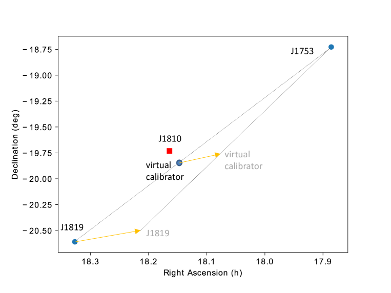
Apart from the 14 new VLBA observations, we re-visited two archival VLBA observations of J1810 taken in 2006 under the project code BH142 and BH145A (Helfand07). An overview of observation dates is provided in 3.2. The two observations in 2006 were carried out at both 5 GHz and 8.4 GHz, using J1753 as the only phase calibrator. More details of the observing setup for the two observations in 2006 can be found in Helfand07. Hereafter, where unambiguous, positions obtained from the two epochs in 2006 and the 14 new epochs are equally referred to, respectively, as the “year-2006 positions” and the “recent positions”.
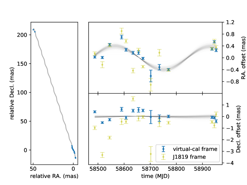
3.4 Data reduction
All VLBI data were reduced with the psrvlbireduce (https://github.com/dingswin/psrvlbireduce) pipeline written in python-based ParselTongue (Kettenis06). ParselTongue serves as an interface to interact with AIPS (Greisen03) and DIFMAP (Shepherd94). The pipeline has been incrementally developed for VLBI pulsar observations over the last decade, notably for the large VLBA programs (Deller19) and (e.g. Ding20).
For the two year-2006 epochs, only data taken at 5 GHz were reduced and analyzed, in order to avoid potential position uncertainties due to any frequency-dependent core shift in the phase calibrators (e.g. Bartel86; Lobanov98). All positions of J1810 were obtained from the gated J1810 data, the S/N of which exceed the ungated J1810 data by 40% on average.
Due to multi-path scattering caused by the turbulent ISM along the line of sight to J1810 or J1819, the deconvolved angular size of J1810 is mildly broadened by mas (detailed in the Appendix), and J1810 (as well as J1819) is fainter at longer baselines. In addition, J1819 exhibits intrinsic source structure, with a jet-like feature extending over 10 mas. Accordingly, J1819 is heavily resolved by the longest baselines of the VLBA, with a flux density of at most a couple of mJy on baselines longer than 50 M (mega-wavelength). The three stations furthest from the geographic centre of VLBA are MK (Mauna Kea), SC (St. Croix) and HN (Hancock), each of which only has 0–1 baselines shorter than 50 M. Unsurprisingly, we found that while valid solutions could still often be found, the phase solutions for HN, MK, and SC are much noisier than for the remainder of the array. On top of this, atmospheric fluctuation causes larger phase variation at longer baselines, which, combined with the worse phase solutions, makes phase wraps (to be explained in 3.4.1) at MK, SC and HN hard to determine. We found that the image S/N for J1810 generally improves when MK, SC and HN are excluded from the target field data, and as a result, taking the three stations out of the J1810 data leads to a statistical positional error comparable to that obtained when using the full array. Therefore, we consistently flagged the three stations from the final J1810 data for 14 recent epochs. However, we did not remove the three stations from any calibration steps, because we found the participation of the three stations allows better performance of self-calibration on J1819 at other stations.
The applied calibration steps in this work are largely the same as the project (Deller19) except for the phase calibration. For the two year-2006 epochs, the phase solutions obtained with J1753 were directly transferred to J1810; whereas, for the recent 14 epochs, phase solutions were corrected based on the positions of J1753 and J1819, before being applied to J1810. Such a technique, though previously adopted by other researchers (e.g. Fomalont03), is applied to a pulsar for the first time.
3.4.1 Dual-calibrator phase calibration
During the phase calibration of VLBI data, the calibration step provides an increment of the phase difference between the station and the reference station in the VLBI array at a given time (for simplicity, frequency-dependency is not accounted for), which is then added to the previous sum of the phase difference when the new solutions are applied. The phase calibration of the primary phase calibrator (J1753 for this work) is followed by the self-calibration of the secondary phase calibrator (J1819 for this work), the phase solutions of which are predominantly limited by anisotropic atmospheric (including ionosphere and troposphere) propagation effect. Accordingly, the position-dependent phase difference should be formulated as , where represents the 2-D sky position. In the normal phase calibration, the solutions obtained with the self-calibration of the secondary phase calibrator at are directly given to the target. The closer is to the target field, the better can approximate the unknown at the target field. In cases where is ∘ away from the target field, considerable offsets are expected between and (especially at lower frequencies), which are commonly treated as systematic errors when using the normal phase calibration. However, if the primary phase calibrator, secondary phase calibrator and the target happen to be quasi-colinear on the sky, can be well approximated by phase solutions corrected from (Fomalont03).
It is easy to prove that for three arbitrary different co-linear positions , and ,
| (3.1) |
assuming higher-than-first-order terms are negligible (as supported by Chatterjee04; Kirsten15). Specific to the self-calibration of the secondary phase calibrator, we have , where and refer to the position of the primary phase calibrator and secondary phase calibrator, respectively; this relation allows us to extrapolate to at any position colinear with J1753 and J1819 based on .
We calculated the closest position to J1810 on the J1753-to-J1819 geodesic line (an arc), where it can best approximate . Since it acts like a phase calibrator for J1810, hereafter we term it the “virtual calibrator” for J1810. The position of the virtual calibrator is , which is 125 away from J1810 (see 3.1). Accordingly, the phase solutions extrapolated to the virtual calibrator are ; using this relation, we corrected the phase solutions of J1819 obtained with its self-calibration. The correction was implemented with a dedicated module called calibrate_target_phase_with_two_colinear_phscals that was newly added to the vlbatasks.py, as a part of the psrvlbireduce package. One of the functions of the module is to solve the phase ambiguity of prior to multiplying by 0.62.
The biggest challenge of the dual-calibrator phase calibration is the phase ambiguity of , which can be equivalently expressed as . This phase ambiguity will not change the quality of solutions for the normal phase calibration, but will cause trouble for the dual-calibrator phase calibration, as the periodicity of the phase is broken when multiplied by a factor. The degree of phase ambiguity depends on observing frequency and angular distance between the main and secondary phase calibrator; for this work (5.7 GHz, 6.5∘), we run into mild phase ambiguity, mainly at the longest baselines (that we do not use anyway as mentioned earlier in this section). Among the recent epochs, the smallest size of the synthesized beam excluding MK, SC and HN is mas, more than two times larger than the level of the systematic uncertainties dominated by propagation effect (see 3.2). Therefore, for this work, we consider less likely to turn more than one wrap, and impossible to turn more than two wraps (i.e. ).
We resolved the phase ambiguity of in a semi-automatic and iterative manner. The pipeline would go though all values of at each station. If holds true throughout the observation, then the solutions are deemed phase-unambiguous, and no human intervention is needed for the station . Otherwise, solutions are plotted out for inspection and interactive correction. In most cases, no interactive correction is necessary after the inspection of the plot, as the solutions look continuous, oscillating around 0 within a reasonable range (e.g. between ). In the few cases where interactive corrections are needed, solutions are ambiguous in phase for at most 1 or 2 stations per observation. This enabled us to take a simple, brute-force approach to trialing the plausible possibilities for phase wraps (adding or subtracting an integer multiple by radians to the solution) with interactive correction. For every possibility, we implemented the dual-calibrator phase calibration using the resultant solution and ran through the complete (data-reduction and imaging) pipeline. The correct should outperform other possibilities in terms of the image S/N for J1810 (and the S/N difference is normally significant), as it better approximates the . This S/N criterium helps us find the “real” , thus the right . The obtained solutions were then transferred to J1810.
More generally, if no phase-calibrator pair quasi-colinear with the target is found, one can extrapolate to at any position with three non-colinear phase calibrators (also known as 2-D interpolation, Fomalont03; Rioja17). Despite the longer observing cycle and hence sparser time-domain sampling (unless using the multi-view observing setup, Rioja17), the tri-calibrator phase calibration can in principle remove all the first-order position-dependent systematics.
3.5 Systematic Errors and Astrometric Fits
3.5.1 Reference frames in relative VLBI astrometry
Similar to the way a reference frame is normally defined in non-relativistic (Cartesian) contexts, a reference frame in the context of relative VLBI astrometry (hereafter reference frame or frame) generally refers to a system of an infinite amount of sky positions that are tied to a phase calibrator (not necessarily a real one), in which positions are measured relative to the phase calibrator. In this work there are three different reference frames where we can measure the positions of J1810: the J1753 frame, the J1819 frame, and the virtual-calibrator frame. To be more specific, in the J1753/J1819 frame, the positions are measured relative to the brightest spot of the model image for J1753/J1819 respectively. By applying an identical model of J1753/J1819222available at https://data-portal.hpc.swin.edu.au/dataset/calibrator-models-used-for-vlba-astrometry-of-xte-j1810-197 during the fringe fitting and self-calibration steps, the J1753/J1819 images at different epochs are aligned, respectively, to and ; the virtual-calibrator frame is thus anchored to , determined by the relation . For the 14 recent epochs, the final positions of J1810 were measured in the virtual-calibrator frame, though the positions of J1810 were also measured in the other two frames for various purposes (see 3.5.2 and 3.2). The two year-2006 positions were merely measured in the J1753 frame, as J1753 is the only available phase calibrator for these observations.
3.5.2 Systematic errors and frame transformation
Similar to the way in which systematic positional errors for pulsars in the project were evaluated using Eqn 1 of Deller19 to account for both differential ionospheric propagation effects and thermal noise at secondary phase calibrators, the estimation of systematic uncertainty for the measured positions of J1810 is based on the mathematical formalism
| (3.2) |
where is the ratio of the systematic error to the synthesized beam size, stands for elevation angle, is the average for a given observation (over time and antennas), is the angular separation between J1810 and the calibrator of the frame, represents the image S/N of the calibrator of the frame, and and are coefficients to be determined. However, unlike Eqn 1 of Deller19, in 3.2 the two contributing terms on the right side are added in quadrature. Given that they should be uncorrelated, this is more appropriate than the linear summation in Eqn 1 of Deller19.
For this work, the second term of 3.2 is negligible for any of the three frames, as both J1753 and J1819 are strong sources, with a brightness 24 at our typical resolution (after MK, SC and HN have been removed from the array). In order to find a reasonable estimate of for this work, we measured the positions of J1810 consistently in the J1753 frame for all 16 epochs, and determined the value of that renders an astrometric fit (see “direct fitting” in 3.5.3) with unity reduced chi-square, or . We obtained . We note that, in principle, is invariant with respect to different reference frames. As is mentioned in 3.5.1, the final positions of J1810 were measured in the virtual-calibrator frame for the 14 recent epochs and in the J1753 frame for the two year-2006 epochs. Using and 3.2 without the second term, we acquired systematic errors for each epoch, which was then added in quadrature to the random errors.
After the determination of the systematic errors, the next step is to transform positions into the same reference frame. Since J1753 and J1819 are remote quasars almost static in the sky, the frame transformation is simply translational. We translated the two year-2006 positions measured from the J1753 to the virtual-calibrator frame. The translation is equivalent, but in the reverse direction, to translate from the virtual-calibrator frame to the J1753 frame, which is easier to comprehend. In order to translate the virtual-calibrator frame to the J1753 frame, the position of the virtual calibrator needs to be measured in the J1753 frame, which can be accomplished by measuring the position of J1819 in the J1753 frame. The method to estimate the position of J1819 and its uncertainty in the J1753 frame is detailed in Section 3.2 of Ding20.
As is shown in 3.1, once is measured in the J1753 frame, the new position of the virtual calibrator in the J1753 frame is also determined, the uncertainty of which is 0.62 times . The difference between and (or 0.62 times the difference between and ) was used to translate the two year-2006 positions of J1810 from the J1753 frame to the virtual-calibrator frame. The was added in quadrature to the error budget (already including systematic and random errors) of the two year-2006 positions.
3.5.3 Proper motion, parallax and distance
After including the systematic errors and unifying to the virtual-calibrator frame, the 16 positions of J1810 can be used for astrometric fitting. Astrometric fitting was performed using pmpar333https://github.com/walterfb/pmpar. The median among the 16 epochs, MJD 58645, was adopted as the reference epoch. The results out of direct fitting are reproduced in 3.1, the of which is 10.6. The large suggests the systematic errors for the recent 14 positions are probably under-estimated, and the actual uncertainty for either parallax or proper motion is about 3 times larger than the uncertainty from direct fitting.
Applying a bootstrap technique to astrometry can generally provide more conservative uncertainties, compared to direct fitting (e.g. Deller19). In the same way as is described in Section 3.1 on Ding20, we bootstrapped 100000 times, from which we assembled 100000 fitted parallaxes, proper motions and reference positions for J1810. The marginalized histograms for parallax and proper motion as well as their paired error “ellipses” are displayed in 3.3. We reported the most probable value at the peak of each histogram as the measured value; the most compact interval containing 68% of the sample was taken as the 68% uncertainty range of the measured value (see 3.3). The parallax and proper motion estimated with bootstrap are listed in 3.1, which are highly consistent with direct fitting while over 3 times more conservative (as is expected from the of direct fitting). Thus, the precision achieved for parallax and proper motion gauged with bootstrap can be deemed reasonable. The parallax corresponds to the distance kpc. Compared to the final 8 parallax, normal phase calibration (in the J1819 frame) would render a consistent parallax with only significance (see 3.2).
| method | References | ||||
|---|---|---|---|---|---|
| () | () | (mas) | (kpc) | ||
| direct fitting | this work | ||||
| bootstrap | this work | ||||
| Previous VLBI astrometry | Helfand07 | ||||
| red clump stars | Durant06 | ||||
| neutral hydrogen absorption | 3.14.0 | Minter08 |
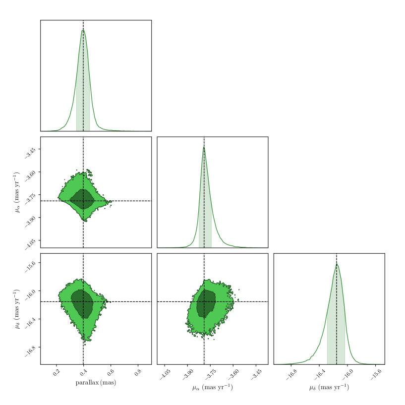
3.5.4 Absolute position
Along with proper motion and parallax, a reference position , mas at the reference epoch MJD 58645 was also obtained for J1810 with bootstrap. We note again the reference position was measured in the virtual-calibrator frame. According to the relation , change in or would cause the position shift of the virtual calibrator (hence the position of J1810), following the relation
| (3.3) |
Using 3.3 and the method outlined in Section 3.2 on Ding20, the reference position was shifted to align with the latest positions of J1753 and J1819444http://astrogeo.org/vlbi/solutions/rfc_2020b/rfc_2020b_cat.html. The shifted reference position mas is the absolute position of J1810 at MJD 58645, where the uncertainties of the J1753 and J1819 positions have been propagated onto the uncertainty budget. At 5.7 GHz, the effect of frequency-dependent core shift (e.g. Bartel86; Lobanov98) is at the mas level in each direction (Sokolovsky11), which makes unnoticeable difference to the uncertainty of the absolute position.
3.6 Discussion
As is shown in 3.1, our new proper motion significantly improves on the previous value inferred from the two year-2006 positions; the new distance kpc is consistent with kpc estimated using red clump stars (Durant06), while in mild tension with 3.14.0 kpc constrained with neutral-hydrogen absorption (Minter08), suggesting the distance to the neutral-hydrogen screen was over-estimated.
In models of NS kicks from the electromagnetic rocket effect (Harrison75) one might expect magnetars to have higher velocities (Duncan92). Our new parallax and proper motion corresponds to the transverse velocity . Using the Galactic geometric parameters provided by Reid19 and assuming a flat rotation curve between J1810 and the Sun, the peculiar velocity (with respect to the neighbourhood of J1810) perpendicular to the line of sight was calculated to be and . Our refined astrometric results consolidate the conclusion by Helfand07 that J1810 has a peculiar velocity typically seen in “normal” pulsars, unless its radial velocity is several times larger than the transverse velocity.
3.6.1 SNR Association
The closest cataloged SNR to J1810 is G11.00.0 (Green19)555http://www.mrao.cam.ac.uk/surveys/snrs/, a partial-shell SNR in size (Brogan04; Brogan06). The position of its geometric center is , away from J1810. The latest distance estimate of G11.00.0 by Shan18 is kpc, consistent with our new distance of J1810. Using our astrometric results, we find that the projected position at 70 kyr ago is , about east to the geometric center of G11.00.0. For the above geometric reasons, it is possible that J1810 is associated with G11.00.0.
The plausibility of this potential association can be tested by considering the ages of both J1810 and G11.00.0. The spin-down rate is erratic for J1810 (Camilo07) as well as other magnetars (Archibald15; Scholz17), making the characteristic age an unreliable estimate of the true age for J1810. Over the course of a decade, the changing value of for J1810 has led to the () increasing from 11 kyr (Camilo07) to 31 kyr (Pintore18). While the characteristic age is currently less than the tentative kinematic age that the tentative association would imply, the unreliability of the estimator in the case of magnetars suggests that the association cannot be ruled out on this basis.
From the perspective of G11.00.0, the compactness of the SNR (see Figure 1 of Castelletti16) suggests that it is probably in the Sedov-Taylor stage. In this stage, the relation between the SNR radius and its age can be rewritten from Sedov59 as
| (3.4) |
where the injected energy is expressed in a value typical of spherical SNRs expanding into the Galactic ISM, and the ambient ISM density for the -ray-emitting region including G11.00.0 was required to power the observed -ray emission above 1 TeV at a distance of 2.4 kpc (Castelletti16). At an SNR distance kpc (Shan18), 3.8 pc (corresponding to the angular size along the long axis), which yields kyr using 3.4, consistent with an SNR in the early part of the Sedov-Taylor phase. A of 70 kyr can be made possible with an injected energy 500 times smaller than the typically-assumed value of erg, which is extremely unlikely (Leahy17). Therefore, we conclude G11.00.0 is not directly associated with J1810. This is not too surprising, as less than half of the known magnetar population has a potential SNR association (Olausen14). Additionally, it has been proposed a strong post-birth magnetar wind can accelerate the dissipation of the SNR (Duncan92).
Though G11.00.0 is not directly associated with J1810, the 3-D geometric alignment might not be a coincidence. One explanation for the geometric alignment is: the progenitor star of J1810 has been in orbit with another supergiant companion; and G11.00.0 is the SNR for the “divorced” companion of J1810. In such a scenario, the progenitor of J1810 underwent a supernova explosion kyr ago and became unbound from its original companion. The companion star continued evolving in isolation before itself undergoing a supernova explosion at kyr ago. In this “companion SNR” scenario, assuming the components of the stellar system were formed at approximately the same time, the progenitor of J1810 should be slightly more massive than its companion (and hence evolve faster). However, given that this scenario would require that the companion underwent a supernova explosion only kyr (compared to the typical supergiant age of Myr) after the first supernova, the mass difference of the two progenitor stars would have to be small.
Assuming no peculiar velocity of the progenitor binary system (with regard to its neighbourhood mean) as well as a flat rotation curve between the Sun and J1810, the expected proper motion of the barycentre of the supergiant binary as observed from the Earth is only 1.2 . The additional proper motion of the companion due to the orbital motion at the moment of unbinding is even smaller for supergiant binaries. Thus, the accumulated position shift of the companion star after the unbinding is at the level across 67 kyr, which does not violate the premise of the “companion SNR” scenario.
In principle, given the large age scatter of supergiants, the “companion SNR” scenario allows J1810 to be indirectly associated with an SNR further away. For example, J1810 can be traced back to 17’ west to the centre of SNR G11.40.1 (which is though far from the boundary of the SNR) at kyr ago. However, the relatively small characteristic age –31 kyr favors the closer indirect association (or no association) with G11.00.0. Despite the “companion SNR” scenario, we note that it is highly possible that J1810 does not come from the G11.00.0 region; instead, it comes from an already dissipated SNR between J1810 and G11.00.0 (as supported by Duncan92). Longer-term monitoring with timing observations on J1810 will offer a more credible range of to be compared with the tentative kinematic age kyr suggested by the possible “indirect” association between G11.00.0 and J1810. Besides, a deeper search for SNR in the narrow region between J1810 and G11.00.0 might provide an alternative candidate for the SNR associated with J1810.
Acknowledgements
We thank Marten van Kerkwijk for his in-depth review and helpful comments on this paper. H.D. is supported by the ACAMAR (Australia-ChinA ConsortiuM for Astrophysical Research) scholarship, which is partly funded by the China Scholarship Council (CSC). A.T.D is the recipient of an ARC Future Fellowship (FT150100415). S.C. acknowledges support from the National Science Foundation (AAG 1815242). Parts of this research were conducted by the Australian Research Council Centre of Excellence for Gravitational Wave Discovery (OzGrav), through project number CE170100004. This work is based on observations with the Very Long Baseline Array (VLBA), which is operated by the National Radio Astronomy Observatory (NRAO). The NRAO is a facility of the National Science Foundation operated under cooperative agreement by Associated Universities, Inc. Data reduction and analysis was performed on OzSTAR, the Swinburne-based supercomputer. This work made use of the Swinburne University of Technology software correlator, developed as part of the Australian Major National Research Facilities Programme and operated under license.
Data and code availability
The pipeline for data reduction is available at https://github.com/dingswin/psrvlbireduce.
All VLBA data used in this work can be found at https://archive.nrao.edu/archive/advquery.jsp under the project codes bd223, bd231, bh142 and bh145a.
The calibrator models for J1753 and J1819 can be downloaded from
https://data-portal.hpc.swin.edu.au/dataset/calibrator-models-used-for-vlba-astrometry-of-xte-j1810-197.
Appendix: Measuring scatter-broadened size of XTE J1810–197
The angular size of a radio source can be measured from its image deconvolved by the synthesized beam. As magnetars are point-like radio sources, a non-zero deconvolved angular size of J1810 can be attributed to scatter-broadening effect caused by ISM. For each epoch, the deconvolved image of J1810 is obtained as an elliptical gaussian component; the mean of its major- and minor-axis lengths is used as the scatter-broadened size of J1810. Assuming the degree of scatter-broadening did not vary across the 14 recent epochs, the 14 measurements of scatter-broadened sizes yield a scatter-broadened size of mas for J1810.
Chapter 4 Probing magnetar formation channels with high-precision astrometry
This chapter is converted from Ding23a entitled “Probing magnetar formation channels with high-precision astrometry: The progress of VLBA astrometry of the fastest-spinning magnetar Swift J1818.01607”, which is the written submission for the International Astronomical Union Symposium 363 with the theme “Neutron Star Astrophysics at the Crossroads: Magnetars and the Multimessenger Revolution”. 4.2 lays out the main scientific motivation of high-precision magnetar astrometry for this thesis, which is to probe magnetar formation channels (also see 1.3.2). The new astrometric results measured for Swift J1818.01607 (see 4.3) and XTE J1810197 (see 4) mark two steps closer to fulfilling the scientific motivation. As an interesting analogy, the space velocity distribution of millisecond pulsars (MSPs) can likely be used to probe the formation channels of MSPs (see 8.7.2 and explanations in 1.3.1).
4.1 Abstract
Boasting supreme magnetic strengths, magnetars are among the prime candidates to generate fast radio bursts. Several theories have been proposed for the formation mechanism of magnetars, but have not yet been fully tested. As different magnetar formation theories expect distinct magnetar space velocity distributions, high-precision astrometry of Galactic magnetars can serve as a probe for the formation theories. In addition, magnetar astrometry can refine the understanding of the distribution of Galactic magnetars. This distribution can be compared against fast radio bursts (FRBs) localized in spiral galaxies, in order to test the link between FRBs and magnetars. Swift J1818.01607 is the hitherto fastest-spinning magnetar and the fifth discovered radio magnetar. In an ongoing astrometric campaign, we have observed Swift J1818.01607 for one year using the Very Long Baseline Array, and have determined a precise proper motion as well as a tentative parallax for the magnetar.
4.2 Introduction
As the most magnetized objects in the universe, magnetars may account for at least 12% of the neutron star population (Beniamini19). However, only roughly 30 magnetars have been identified (Olausen14) in our Galaxy or in the Magellanic Clouds. This discrepancy can be explained by short-lived energetic electromagnetic activities of magnetars.
Magnetars sit at the intersection of multiple research topics. Their postulated link to fast radio bursts (FRBs) has been strengthened by the FRB-like bursts recently observed from a Galactic magnetar (Andersen20; Bochenek20). But it remains unclear whether all FRBs are originated from magnetars. Magnetars are also strongly connected to -ray bursts (GRBs) through the detection of giant magnetar flares from nearby galaxies (e.g. the one in NGC 253, Roberts21; Svinkin21), and newborn magnetars from double neutron star mergers (e.g. Sarin21). On the other hand, the formation mechanism of magnetars is yet not well understood. A few distinct magnetar formation theories have been proposed, including normal core-collapse supernovae (CCSN) of magnetic massive stars (Schneider19), accretion-induced collapse (AIC) of white dwarfs (Duncan92) and double neutron star mergers (Giacomazzo13; Xue19). Most magnetar formation channels require magnetars to be born with millisecond spin periods. The only exception is the normal CCSN formation channel, where a new-born magnetar simply inherits the magnetic fields from its magnetic progenitor star (Schneider19).
While almost all magnetars are identified with their soft -ray and X-ray activities, % of them are also visible at optical/infrared or radio frequencies (Olausen14). This visibility allows precise astrometry for the magnetars. Historically, 7 magnetars have been precisely measured astrometrically, including 4 infrared-bright magnetars (Tendulkar13) and 3 radio magnetars (Deller12a; Bower15; Ding20c). The primary motivations of previous astrometric campaigns of magnetars are to 1) establish supernova remnant associations and 2) test whether magnetars receive extraordinary kick velocities ( ) as predicted by Duncan92. With growing numbers of Galactic magnetars precisely measured astrometrically, new research opportunities start to emerge.
The small sample studied by Tendulkar13, entailing 6 astrometrically measured magnetars, offers no indication that magnetar space velocities (magnetar velocity with respect to the neighbourhood of the magnetar) follow a distribution different from that of normal pulsars (Hobbs05). This rough consistency may imply that most magnetars in spiral galaxies are born in normal CCSN similar to the ones that create typical neutron stars. The CCSN origin of magnetars is also supported by few SNR associations of magnetars (e.g. Borkowski17, GCN circular 16533). On the other hand, the DNS merger origin is not favored by the Galactic magnetar sample, as all Galactic magnetars are found near the Galactic plane (see 4.1). For other formation channels (e.g., the AIC channel), it remains an open question if they contribute to the formation of the Galactic magnetar population, or more generally magnetars in spiral galaxies. This question can be approached with a refined magnetar space velocity distribution, to be established with 10 Galactic magnetars precisely measured astrometrically. As different formation channels may lead to distinct magnetar space velocity distributions (e.g., the AIC channel would probably give rise to relatively small magnetar space velocities), the averaged magnetar space velocity distribution could turn out to be bi-modal or even multi-modal (if there are more than one formation channel of magnetars).
Astrometry of Galactic magnetars would also play a role in the FRB study. On one hand, FRBs have been localized to specific environments (i.e., spiral arms) of spiral galaxies (Mannings21). On the other hand, magnetar astrometry could potentially pinpoint the 3-D magnetar location (Ding20c) in the Galaxy. Hence, comparing the Galactic magnetar distribution against FRB sites (localized to spiral galaxies) can test the link between FRBs and magnetars. However, Galactic magnetars precisely measured astrometrically are usually limited to the vicinity of the Solar system. To better infer magnetar distributions in spiral galaxies, one needs the knowledge of contributing formation channels of magnetars in the spiral galaxies (which, again, can be approached by magnetar astrometry). This is because magnetars formed in one channel are expected to follow a specific spatial distribution (e.g., magnetars born via the CCSN and DNS-merger channel are expected to be associated with, respectively, star-forming regions and stellar mass of a galaxy).
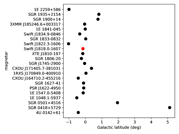
4.3 The progress of astrometry of Swift J1818.01607
Swift J1818.01607 is the fifth discovered radio-bright (Karuppusamy20) magnetar (GCN circular 27373), which is also the hitherto fastest-spinning magnetar with a spin period of 1.4 s (Enoto20). Its short spin period and high spin-down rate correspond to a characteristic age of around 500 yr (champion20a), implying its great youth. Right after the radio detection of Swift J1818.01607, we launched an astrometric campaign of the magnetar using the Very Long Baseline Array (VLBA). The first VLBA observation was made at 1.6 GHz on 20 April 2020, which did not lead to a detection (Ding20b). In response to the spectral flattening (of Swift J1818.01607) first noticed in July 2020 (e.g. Majid20), we raised the observing frequency to 8.8 GHz, and managed to detect Swift J1818.01607 with VLBA on 19 August 2020 (Ding20b).
At the time of writing, more than a year has passed since the first VLBA detection. During this period, 5 more VLBA observations have been made, all resulting in detections at sub-mas positional precision. We applied pulsar gating to improve image S/N, where the pulse ephemerides were generated from ongoing Parkes monitoring of Swift J1818.01607 (Lower20c). To enhance astrometric accuracy of our observations, we have employed the 1-D interpolation tactic (e.g. Fomalont03; Ding20c) for all the 6 VLBA observations. After data reduction and analysis, we obtained a compelling proper motion , , alongside a tentative (5 ) parallax (see 4.2). Here, in order to roughly account for the systematic errors caused by atmospheric propagation effects, the uncertainty of the proper motion (as well as parallax) has been scaled by , where stands for reduced chi-square of direct parallax fitting. The final astrometric results with thorough error estimation will be obtained and discussed in a future publication, following the completion of the whole astrometric campaign that spans at least 2 years.

4.4 Future prospects
For Swift J1818.01607, with 6 more VLBA observations to be made in the following year, the parallax measurement is likely to become substantial (), which would simplify the conversion of parallax to distance (without needing to take into account the Lutz-Kelker effect, Lutz73). With regard to the whole magnetar category, to establish the magnetar space velocity distribution is mainly limited by the small sample of (, Olausen14) radio or optical/infrared magnetars. To expand this sample and hence accelerate the establishment of the magnetar space velocity distribution, new candidates of radio or optical/infrared magnetars, such as the newly discovered ultra-long-period sources (e.g. Hurley-Walker22), are desired.
Chapter 5 Testing the models of photospheric radius expansion bursts with Gaia parallaxes
This chapter is transformed from Ding21 entitled “Gaia EDR3 parallaxes of type I X-ray bursters and their implications on the models of type I X-ray bursts: A generic approach to the Gaia parallax zero point and its uncertainty”. The type I X-ray bursters (bursters) studied in this chapter are a subset of the neutron star (NS) X-ray binary (XRB) population, and will eventually evolve into recycled pulsars (which are the focus of 6, 7 and 8) after the phase of active accretion (see 1.1.4).
This is the only paper chapter based on Gaia data (see 1.2.1 for a summary of methods of high-precision astrometry). The Gaia sources (see 5.1) identified for the 4 bursters are the optically bright donor stars of the XRB systems (see 1.1.4). Among the 4 bursters, radio emissions have only been reported for Cyg X2 (e.g. Hjellming90; Spencer13). Hence, Gaia astrometry serves as the major pathway to fulfilling the scientific goal of this chapter. Provided the relatively large distances to the 4 bursters, the position shift due to orbital motion is too small to affect the Gaia astrometric fitting performance (see 2.3).
5.1 Abstract
Light curves of photospheric radius expansion (PRE) bursts, a subset of type I X-ray bursts, have been used as standard candles to estimate the “nominal PRE distances” for 63% of PRE bursters (bursters), assuming PRE burst emission is spherically symmetric. Model-independent geometric parallaxes of bursters provide a valuable chance to test models of PRE bursts (PRE models), and can be provided in some cases by Gaia astrometry of the donor stars in bursters. We searched for counterparts to 115 known bursters in the Gaia Early Data Release 3, and confirmed 4 bursters with Gaia counterparts that have detected (, prior to zero-point correction) parallaxes. We describe a generic approach to the Gaia parallax zero point as well as its uncertainty using an ensemble of Gaia quasars individually determined for each target. Assuming the spherically symmetric PRE model is correct, we refined the resultant nominal PRE distances of three bursters (i.e. Cen X4, Cyg X2 and 4U 091954), and put constraints on their compositions of the nuclear fuel powering the bursts. Finally, we describe a method for testing the correctness of the spherically symmetric PRE model using parallax measurements, and provide preliminary results.
5.2 Introduction
A type I X-ray burst is rapid nuclear burning on the surface of a neutron star (NS) (e.g. Lewin93). Type I X-ray bursts happen when the accumulated “nuclear fuel” accreted from the donor star onto the surface of the NS is sufficiently hot. In some cases, the radiation pressure becomes large enough to overcome the gravity of the NS, causing the photosphere to expand. This is followed by fallback of the photosphere after extending to its outermost point. This process of expansion and contraction of the photosphere is well characterised by double-peaked soft X-ray light curves. These particular type I X-ray bursts are called photospheric radius expansion (PRE) bursts.
According to Galloway20, there are hitherto 115 recognized PRE bursters (see https://burst.sci.monash.edu/sources), which are all low mass X-ray binaries (LMXBs). PRE bursts can serve as standard candles (Basinska84) based on the assumption that the luminosity of PRE bursts stays at the Eddington limit throughout the photospheric expansion and contraction. We refer to the distances estimated in this way as PRE distances. Using the standard assumption of spherically symmetric PRE burst emission, Galloway20 constrained PRE distances for 73 PRE bursters (23 of which only have upper limits of PRE distances, see Table 8 of Galloway20) based on the theoretical Eddington luminosity calculated by Lewin93. Hereafter, we refer to this spherically symmetric model as the simplistic PRE model, and the simplistic-PRE-model-based PRE distances as nominal PRE distances. Besides PRE models, a Bayesian framework has been recently developed to infer parameters, including the distance and the composition of nuclear fuel on the NS surface, for the type I X-ray burster SAX J1808.43658 (Goodwin19), by matching the burst observables (such as burst flux and recurrence time) of non-PRE type I X-ray bursts with the prediction from a burst ignition model (Cumming00).
At least 43% of PRE bursters registered nominal PRE distances as their best constrained distances. The great usefulness of the simplistic PRE model calls for careful examination of its validity. There are several uncertainties in the simplistic PRE model. Firstly, according to Lewin93, the Eddington luminosity measured by an observer at infinity
| (5.1) |
depends on the NS mass and the gravitational redshift (where and stand for Newton’s gravitational constant and speed of light in vacuum, respectively) at the photosphere radius . To a greater degree, hinges on the hydrogen mass fraction of the nuclear fuel on the NS surface at the time of the PRE burst: hydrogen-free nuclear fuel corresponds to a 1.7 times higher than nuclear fuel of cosmic abundances (Lewin93). Secondly, the method assumes spherically symmetric emission. On one hand, PRE bursts per se are not necessarily spherically symmetric given that the NS in an LMXB is spinning and accretes via an accretion disk. On the other hand, even if PRE bursts are initially isotropic (assuming the nuclear fuel has spread evenly on the NS surface), propagation effects (such as the reflection from the surrounding accretion disk) would still potentially lead to anisotropy of PRE burst emission. Thirdly, for each PRE burster, the peak fluxes of its recognized PRE bursts vary, typically by 13% (Galloway08).
Provided the uncertainties of the simplistic PRE model as well as the resultant nominal PRE distances, independent distance measurements for PRE bursters hold the key to testing the simplistic PRE model. By 2003, 12 PRE bursters in 12 globular clusters (GCs) had distances determined from RR Lyrae stars residing in the GCs; incorporating the distances with respective peak bolometric fluxes derived from X-ray observations of PRE bursts, Kuulkers03 measured 12 observed Eddington luminosities, 9 of which are consistent with the theoretical value by Lewin93. The independent check by Kuulkers03 largely confirms the validity of the simplistic PRE model. The confirmation, however, is not conclusive due to the modest number of PRE bursters residing in GCs. Besides, this GC-only sample of PRE bursters might lead to some systematic offsets of the measured Eddington luminosities, as a result of potential systematic offsets of distances determined with RR Lyrae stars or X-ray flux decay that becomes more prominent in the dense regions of GCs.
Alternatively, geometric parallaxes of PRE bursters provided by the Gaia mission (Gaia-Collaboration16) can also be used to test the simplistic PRE model. This effort normally requires determination of Gaia parallax zero point for each PRE burster, as is found to be offset from 0 (Lindegren18; Lindegren21). Recently, Arnason21 (A21) has identified Gaia Data Release 2 (DR2) counterparts for 10 PRE bursters with Gaia parallaxes. After applying the Gaia DR2 global (Lindegren18), A21 converted these parallaxes into distances, incorporating the prior information described in Bailer-Jones18. A21 noted that the inferred distances of the 10 PRE bursters are systematically smaller than the nominal PRE distances estimated before 2008 (this discrepancy is relieved with the latest nominal PRE distances by Galloway20, see the discussion in 5.5.2). However, due to the predominance of low-significance parallax constraints, this discrepancy is strongly dependent on the underlying Galactic distribution of PRE bursters (as is shown in Figure 3 of A21), which is far from well constrained. Moreover, adopting the Gaia DR2 global , instead of one individually estimated for each source, would introduce an extra systematic error.
This work furthers the effort of A21 to test the simplistic PRE model with Gaia parallaxes of PRE bursters, making use of the latest Gaia Early Data Release 3 (EDR3, Brown21). Unlike A21, this work only focuses on the PRE bursters with relatively significant Gaia parallaxes; we apply a locally-determined for each PRE burster, and probe the simplistic PRE model as well as the composition of nuclear fuel.
In addition to the above-mentioned motivation, Gaia astrometry of PRE bursters (hereafter simplified as bursters, when unambiguous) can provide more than geometric parallaxes (and hence distances). A Gaia counterpart of a burster also brings a reference position precise to sub-mas level, and possibly a detected proper motion as well. The latter can be combined with the parallax-based or model-dependent distance estimates to yield the burster’s transverse space velocity (the transverse velocity with respect to its Galactic neighbourhood). The space velocity distribution of PRE bursters (or LMXBs) is important for testing binary evolution theories (see Tauris17 as an analogy). Both reference position and proper motion can be used to confirm or rule out candidate counterparts at other wavelengths, especially when the immediate neighbourhood of a burster is crowded on a 1” scale.
In this paper, all uncertainties are quoted at the confidence level unless otherwise stated; all sky positions are J2000 positions. As we mainly deal with Gaia photometric passbands (Jordi10) in this work, a conventional optical passband is referred to in the form of , while its magnitude is denoted by ; by contrast, a Gaia passband is referred to in the form of Y band, and its magnitude is denoted by .
5.3 Gaia counterparts of PRE bursters with detected parallaxes
To be able to effectively refine nominal PRE distances, constrain the composition of nuclear fuel on the NS surface and test the simplistic PRE model, we only search for Gaia counterparts with detected parallaxes (, a criterion we apply throughout this paper). This cutoff leads to a smaller sample of PRE bursters compared to A21, which included many marginal parallax detections. Our search is based on the positions of 115 PRE bursters compiled in Table 1 of Galloway20. For each PRE burster, we found its closest Gaia EDR3 source within 100 using TOPCAT111http://www.star.bris.ac.uk/~mbt/topcat/. From the resultant 110 candidates, we shortlisted 16 Gaia counterpart candidates with detected . Among the 16 Gaia counterpart candidates, the Gaia counterparts for Cyg X2, Cen X4 and 4U 091954 have been recognized by VizieR (Ochsenbein00) in an automatic manner, simply based on the mas angular distance (at the reference epoch year 2015.5 disregarding proper motion) that is comparable to the Gaia positional uncertainties (see 5.1); the Gaia counterpart for XB 212947 has been identified by A21.
To identify Gaia counterparts of PRE bursters from the remaining 12 candidates, we adopted a more complicated cross-match criterion, which requires the identification of an optical counterpart (either confirmed or potential) for the PRE burster. For an optical source that is a confirmed or potential counterpart, we consider it associated with the Gaia source if all the following conditions are met:
-
(i)
is sufficiently bright (222https://www.cosmos.esa.int/web/gaia/earlydr3) for Gaia detection; the conventional apparent magnitude measured closest to band is looked at if is not available (as compiled in 5.1);
-
(ii)
falls into the 1--radius circle around (where the position of a confirmed radio or infrared counterpart of would be adopted if it is more precise than the optical position);
-
(iii)
is the only Gaia source within the 5--radius circle around .
Here, to account for the effect of proper motion (and the smaller contribution of parallax), the position of the candidate has been extrapolated to the epoch at which the position of was measured, with the astrometric parameters of using the “predictor mode” of pmpar (available at https://github.com/walterfb/pmpar). This extrapolation allows the evaluation of the same-epoch , the separation between and , which is free from proper motion and parallax effects.
In principle, the apparent magnitude of should match that of the optical counterpart of . However, making such a comparison is complicated by 1) the wide photometric passbands designed for the in-flight Gaia (Jordi10) and 2) magnitude variability of stars.
On top of the 4 Gaia counterparts of PRE bursters (Cen X4, Cyg X2, 4U 091954 and XB 212947) already recognized by VizieR and A21, we identified one Gaia counterpart with detected (from the remaining 12 objects), which was NP Ser (see 5.1). However, as we will discuss in 5.5.1, NP Ser is not the optical counterpart of GX 172, meaning that our final sample consists of 5 Gaia sources with detected , of which 4 are PRE bursters.
Hereafter, the 5 Gaia sources are sometimes referred to as “targets”. The (Gaia) B band covers the conventional , , bands and part of the band. According to 5.1, the magnitude of NP Ser measured at conventional band generally agrees with of its Gaia counterpart. The 5 astrometric parameters of the Gaia counterparts for the 4 PRE bursters and NP Ser are summarized in 5.2.
| source name | Gaia EDR3 | associated | |||||
|---|---|---|---|---|---|---|---|
| (mag) | (”) | counterpart | (mag) | (”) | (”) | by? | |
| NP Ser | 0.5 | 4146621775597340544 | 17.72 | 0.3 | 12 | this work | |
| Cyg X2 | 1952859683185470208 | VizieRi | |||||
| Cen X4 | 6205715168442046592 | VizieRi | |||||
| 4U 091954 | 5310395631798303104 | VizieRi | |||||
| XB 212947 | 1978241050130301312 | A21k |
Apparent magnitude at a conventional passband; positional uncertainty (adding in quadrature uncertainties in both directions) of the source (see 5.3); apparent magnitude at the Gaia B band (Jordi10), which covers the conventional , , bands and part of the band; angular separation between the source and its Gaia counterpart, where and were extrapolated to the respective epoch of (and ) using the astrometric parameters in 5.2 (see 5.3 for more explanation); maximum search radius that contains only one Gaia source.
Deutsch96; Deutsch99, where 380, 14∘02’1134 out of R-band CCD observation, with uncertainty radius of 05 at 90% confidence, measured at MJD 50674.
iOchsenbein00; kArnason21.
| source name | |||||
|---|---|---|---|---|---|
| ( in mas) | (mas) | () | () | ||
| NP Ser | 0.69(8) | 3.35(8) | -6.97(6) | ||
| Cyg X2 | 0.068(19) | -1.79(2) | -0.32(2) | ||
| Cen X4 | 0.53(13) | 0.84(15) | -55.68(13) | ||
| 4U 091954 | 0.24(6) | -5.77(7) | 2.24(8) | ||
| XB 212947 | 0.50(8) | -2.34(8) | -4.23(8) |
5.4 Calibration of Gaia parallaxes
Before being applied for scientific purposes, each of the Gaia parallaxes needs to be calibrated by determining its (Gaia) parallax zero point , as has been shown to be systematically offset from zero (with an all-sky median of mas for EDR3; Lindegren21). Previous studies have revealed the dependence of on sky position, apparent magnitude and color (Lindegren18; Chen18; Huang21). Furthermore, Lindegren21 proposed that the position dependence of can be mostly attributed to the evolution of with respect to ecliptic latitude , and derived an empirical global solution for five-parameter (see Lindegren21a for explanation) Gaia EDR3 sources and another such solution for six-parameter sources. While this approach is convenient to use, the empirical solutions do not provide an estimate of the uncertainty of , and are only considered indicative (Lindegren21).
In this work, we attempted a new pathway of generic determination. Unlike the global empirical solutions, the new determination technique offers locally acquired , and provides the uncertainty of the determined . We estimated for the 5 targets using a subset of the agn_cross_id table publicized along with EDR3 (Klioner et al. in preparation). We selected 1,592,629 quasar-like sources (out of the 1,614,173 sources in the agn_cross_id table), which a) have (denoted as “bp_rp” in EDR3) values and b) show no detected ( level) proper motion in either direction. Hereafter, we refer to this subset of 1,592,629 sources as the quasar catalog, and its sources as background quasars or quasars (when unambiguous).
On the sky, spatial patterns of on angular scales of up to ∘ are seen in Figure 2 of Lindegren21. We attempted different radius cuts (around each of the 5 targets) of up to 40∘, but found no clear evidence showing quasar parallaxes representative of the target beyond a 10∘ radius cut. In most cases, a 10∘ radius cut provides a sufficiently large sample of quasars for estimation. Hence, we only present analysis of quasars within 10∘ around each target.
5.4.1 A new pathway to parallax zero points
Our determination is solely based on the quasar catalog (of 1,592,629 sources). The vital step of (Gaia) parallax calibration (or determination) is to select appropriate quasars in the same sky region with similar G-band apparent magnitudes and colors . We implemented this selection for each of the 5 targets by applying 4 filters to the quasar catalog: the angular-distance filter, the filter, the filter and the filter. Once appropriate background quasars are chosen for each target, one can calculate as the weighted mean parallax of this “sub-sample”, and the formal uncertainty of
| (5.2) |
(Equation 4.19 in Bevington03), where is the (Gaia) parallax error of each background quasar in the sub-sample.
We parameterized 1) the angular-distance filter using the search radius around the target, 2) the filter using , the half width of the filter centred about , 3) the filter using , which stands for the relative half width (or ) of the filter around , and 4) the filter using , the half width of the filter centred about .
Hence, the problem of determination using background quasars can be reduced to searching for optimal filter parameters (for each target), i.e. , , and . For this search, we investigated the marginalized relation between and each of the 4 parameters (see the top 4-panel block of 5.1), where stands for the weighted standard deviation of quasar parallaxes divided by its global value of 0.32 mas. To avoid small-sample fluctuations, 5.1 starts at , or , which can also prevent overly small-sized sub-samples. To start with, we first introduce the -to- relation and explain its implications. Relations between and other 3 parameters can be interpreted in the same way.
Unlike , if a sufficiently large () background-quasar sample had no dependence (as opposed to Lindegren18; Lindegren21), would be expected to be largely independent to , and to fluctuate around the global value 0. This is clearly not the case for all of the 5 targets. From 5.1, we found an obvious upward trend of with growing . This upward trend shows that background quasars with similar around tend to have similar parallaxes, which supports the -dependence of stated in Lindegren18; Lindegren21.
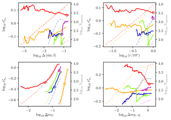
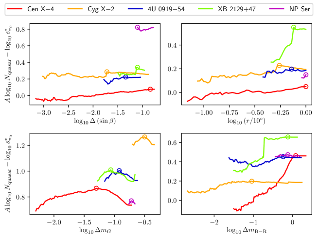
Using the same interpretation, we also investigated marginalized relations of with respect to each of the other 3 filter parameters. As can be seen in 5.1, most fields show a (weak) color dependence of . For the two sky-position-related filter parameters, dependence of is clearly found in the target fields of Cyg X2 and NP Ser, whereas the dependence of is hardly noticeable in any of the 5 target fields. This contrast reinforces the belief that the dependence of contributes considerably to the position dependence of (Lindegren21). Additionally, converges to at in all target fields, which roughly agrees with our assumption that the -dependence of becomes negligible beyond 10∘ search radius; in other words, quasar parallaxes at are almost not representative of the target .
Knowing the way to interpret the relation between and each of the filter parameters, we can proceed to choose the optimal filter parameters. In choosing filter parameters, one wants the filtered sub-sample to have a consistently low level of ; meanwhile, one prefers a filtered sub-sample as large as possible to achieve reliable and precise . To meet both demands is difficult when rises with a larger filter (as is the case for the filter). In this regard, we created an index , where is a scaling factor. Instead of the minimum of or the maximum of , we adopted the filter parameter at the peak of the index (see the bottom 4-panel block of 5.1), so that an optimized trade-off between and can be reached. Using this consistent standard, we reached the parameter of each filter for each target (see 5.3).
After applying the 4 filters, we acquired a quasar sub-sample of and for each target, and obtained of the target from this sub-sample (see 5.3). Due to the relative paucity of quasars identified at low Galactic latitudes (for the reasons discussed in Lindegren21), NP Ser, 4U 091954 and XB 212947 (all of which have ∘) receive relatively low values for compared to Cen X4 (∘), which partly lead to the relatively large . Nonetheless, we have shown that for targets at ∘ can be determined with nearby (on the sky) quasars. On the other hand, Cyg X2, despite being located at ∘, has the smallest and the largest among the 5 targets. This is mainly due to the relative rarity of bright quasars (Cyg X2 has mag).
The negative of the quasar sub-sample for each target indicates that the sub-sample of (closely located, like-, like- and like-) quasars are representative of the target source. Despite this good representativeness, the estimated with 5.2 is still an under-estimate for the uncertainty of , as the sub-sample has a spread in each parameter and does not represent the target perfectly. We estimated the weighted average , and of the quasar sub-sample (where the weighting is , see 5.2 for the definition of ), which are presented in 5.3 as , and , respectively. According to 5.3, there are residual offsets of , and between the target and the average level of the sub-sample, which would result in extra systematic error for the estimates. In order to estimate this systematic error of , we calculated the empirical parallax zero points for the targets (see 5.3) using zero_point.zpt (https://gitlab.com/icc-ub/public/gaiadr3_zeropoint, Lindegren21), noted as . In the same way, we also estimated the empirical parallax zero points for each quasar of the sub-sample, then derived the weighted average empirical parallax zero point of the sub-sample, noted as (see 5.3). The difference between and is taken as an estimate for the systematic error of , which is added in quadrature to the calculated with 5.2.
No uncertainties are yet available for . Regardless, all of our are consistent with the empirical counterparts at the confidence level. We note that is only used to estimate the systematic error of , and is not adopted in the discussions that follow. The calibrated parallaxes are summarized in 5.3.
Despite the overall consistency between and , it is noteworthy that all are larger than the counterparts, which can be a coincidence of small-number statistics. Alternatively, knowing that most of the targets are situated at low , it might indicate a systematic offset between quasar-sub-sample-based and at low . Interestingly, a recent parallax zero-point study based on 110,000 W Ursae Majoris variables showed that the W-Ursae-Majoris-variable-based are systematically larger than the counterparts at low (see Figure 3 of Ren21). Hence, a future quasar-sub-sample-based study involving a large sample of targets (and other parallax zero-point studies by different approaches) will be essential for probing at low . More specifically, if quasar-sub-sample-based at low are confirmed to be systematically larger than the counterparts, then it is likely that is systematically under-estimated at low .
| field | ||||||||||
|---|---|---|---|---|---|---|---|---|---|---|
| (∘) | (mag) | (mag) | (mag) | |||||||
| Cen X4 | 10 | 0.14 | 17.85 | 5.0% | 1.59 | 1.20 | 18.00 | 0.74 | -0.25 | |
| Cyg X2 | 5.5 | 0.74 | 0.02 | 14.70 | 31.6% | 0.71 | 0.09 | 18.19 | 0.74 | 0.74 |
| 4U 091954 | 7.2 | 0.05 | 17.15 | 12.0% | 1.19 | 0.58 | 18.23 | 0.94 | -0.93 | |
| XB 212947 | 7.6 | 0.84 | 0.08 | 17.58 | 8.7% | 1.29 | 0.76 | 18.49 | 1.01 | 0.79 |
| NP Ser | 10 | 0.16 | 0.08 | 17.01 | 19.1% | 1.51 | 0.76 | 17.61 | 1.57 | 0.16 |
| field | |||||||
|---|---|---|---|---|---|---|---|
| (mas) | (mas) | (mas) | (mas) | ||||
| Cen X4 | 772 | ||||||
| Cyg X2 | 32 | ||||||
| 4U 091954 | 91 | ||||||
| XB 212947 | 63 | ||||||
| NP Ser | 40 |
5.5 Discussion
In this section, we discuss the implications of the 5 calibrated parallaxes provided in 5.3.
5.5.1 NP Ser and GX 172 revisited
GX 172 is one of the brightest X-ray sources on the sky, from which 43 PRE bursts have been recorded (see Table 1 of Galloway20 and references therein); its distance was estimated to be 7.3–12.6 kpc by treating its PRE bursts as standard candles (as explained in 5.2), where the distance uncertainty is dominated by the uncertain composition of the nuclear fuel (Galloway20). The optical source NP Ser, away from GX 172, was initially considered the optical counterpart of GX 172 (Tarenghi72); but the association has been ruled out, based on its sky-position offset from GX 172 (Deutsch99) and its lack of optical variability (as expected for the optical counterpart of GX 172) (e.g. Davidsen76; Margon78). Despite this, NP Ser was initially treated as a potential counterpart and the Gaia properties of NP Ser were analysed. Regardless of the non-association of NP Ser and GX 172, the complex sky region around GX 172 for optical/infrared observations (see Figure 2 of Deutsch99 for example) merits high-precision Gaia astrometry of NP Ser, which will facilitate future data analysis of optical/infrared observations of GX 172.
Using the astrometric parameters of NP Ser in 5.2 and 5.3, we extrapolated the reference position of NP Ser (from the reference epoch 2016.0 yr, or MJD 57388) to MJD 47496, following the method described in Section 3.2 of Ding20. The projected Gaia position of NP Ser is offset from the VLA position of GX 172 (see Table 2 of Deutsch99) by 007 at MJD 47496. Considering the distances to GX 172 and NP Ser, nuclear fuel with cosmic abundances (73% hydrogen) corresponds to the smallest PRE distance of kpc for GX 172 (Galloway20); in comparison, the calibrated Gaia parallax of NP Ser is mas, corresponding to a distance of kpc, which establishes NP Ser as a foreground source of GX 172. The current sky-position offset between NP Ser and GX 172 depends on the proper motion of GX 172. Assuming GX 172 rotates around the Galactic centre in the Galactic disk with negligible peculiar velocity (with respect to the neighbourhood of GX 172), the apparent proper motion of GX 172 would be and given a distance of 8.5 kpc (from the Earth). Based on this indicative proper motion of GX 172 and the Gaia ephemeris of NP Ser, NP Ser is currently (at MJD 59394) 10 away from GX 172, and continues to move away from GX 172 on the sky; accordingly, it would become easier with time to resolve GX 172 from the foreground NP Ser in optical/infrared observations.
5.5.2 Posterior distances and compositions of nuclear fuel for Cen X4, Cyg X2 and 4U 091954
Among the (calibrated) parallaxes of the 4 PRE bursters (i.e. Cen X4, Cyg X2, 4U 091954 and XB 212947), for Cen X4, 4U 091954 and XB 212947 are detected, whereas of Cyg X2 is weakly constrained. All PRE bursters except XB 212947 have nominal PRE distances published that are inferred from their respective PRE bursts (see 5.4 for PRE distances and their references). Using Bayesian inference, we can incorporate the parallax of a PRE burster with its nominal PRE distance to constrain the composition of nuclear fuel and refine the nominal PRE distance.
In 5.2, we have mentioned that the Eddington luminosity (measured by an observer at infinity) varies with NS mass and photosphere radius (see 5.1). In practice, the bolometric flux at the “touchdown” (when the photosphere drops back to the NS surface) of a PRE burst is compared to the theoretical at (where stands for NS radius) to calculate the nominal PRE distance (Galloway20). Therefore, the theoretical should change with and , which is, however, not taken into account in this work. We note that, following Galloway20, we assume and km (Steiner18) for all PRE bursters.
Bayes factor between two ends of the composition of nuclear fuel
As mentioned in 5.2, the Eddington luminosity of PRE bursts depends on the composition of nuclear fuel (accreted onto the NS surface from its companion) at the time of the outburst. This composition is normally parameterized by , the mass fraction of hydrogen in nuclear fuel at the time of a PRE burst, which generally ranges from 0 to %, the cosmic mass fraction of hydrogen. As the result of the dynamic nucleosynthesis process during accretion, varies from one PRE burst to another, but is always smaller than the hydrogen mass fraction of the donor star. can be roughly predicted by the theoretical ignition models of X-ray bursts, and mainly depends on the local accretion rate (e.g. Fujimoto81).
Nominal PRE distances for , denoted as , are summarized in 5.4 along with their references. At any given , the nominal PRE distance (Lewin93). As the fractional uncertainty of a nominal PRE distance measurement is independent of , , where and represent the uncertainty of the nominal PRE distance at and at a given , respectively.
As our first attempt to constrain , we used the calibrated Gaia parallax of each PRE burster to determine which value of is more likely for the burster – 0.73 or 0. We calculated the Bayes factor using
| (5.3) |
where , and . For the calculation of , we did not use any Galactic prior (see 5.4 for explanation), as the extra constraint given by a Galactic prior is negligible when is fixed. The results of are presented in 5.4.
Among the three values, the one for Cen X4 is the most offset from 0, which suggests the calibrated parallax of Cen X4 substantially (when , Kass95) favors over . Merely 2 PRE bursts have ever been observed from Cen X4 in 1969 (Belian72) and 1979 (Matsuoka80). The long intervals between PRE bursts of Cen X4 imply small accretion rates and low at the time of PRE bursts, despite hydrogen signatures observed from its donor star (e.g. Shahbaz14). This expectation is confirmed by the of Cen X4.
It is noteworthy that hydrogen-poor nuclear fuel at the time of PRE bursts is also favored for Cyg X2 and 4U 091954. In fact, the previous independent test of the simplistic PRE model using GC PRE bursters also suggests hydrogen-poor nuclear fuel at the time of PRE bursts for the majority of the 12 GC PRE bursters (Kuulkers03). The statistical inclination towards low , if confirmed with a larger sample of PRE bursters, might be partly attributed to a selection effect explained as follows.
For each PRE burster, only the brightest PRE bursts are selected to calculate its nominal PRE distance (Galloway08; Galloway20; Chevalier89). This selection criterion results in a nominal PRE distance that tends to decrease with time as brighter bursts are discovered. This tendency is clearly shown by the fact that almost all the nominal PRE distances registered in Table 9 of Galloway08 are larger than their counterparts in Table 8 of Galloway20. If we assume the variability of observed fluxes of PRE bursts is mainly caused by the fluctuation of (at the time of different PRE bursts), the selection criterion of PRE bursters would lead to an increasingly biased PRE-burst sample that is more likely low-. This selection effect would have a big impact on the of the frequent PRE burster Cyg X2 (see in Table 1 of Galloway20), but less so for 4U 091954 and Cen X4. A low of 4U 091954 (if confirmed in the future) can be explained by the suggestion that the donor star of 4U 091954 is likely a helium white dwarf (int-Zand05). On the other hand, the revised nominal PRE distances of PRE bursters (Galloway20) relieve the tension between the pre-2008 nominal PRE distances (see the references in Table 1 of A21) and the Gaia DR2 distances (A21), as mentioned in 5.2.
| PRE | ||||
|---|---|---|---|---|
| burster | (kpc) | (kpc) | ||
| Cen X4 | 1.2(3) a | |||
| Cyg X2 | 11.6(9) b | |||
| 4U 091954 | 3.9(2) b |
a Chevalier89; b Galloway20.
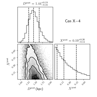 |
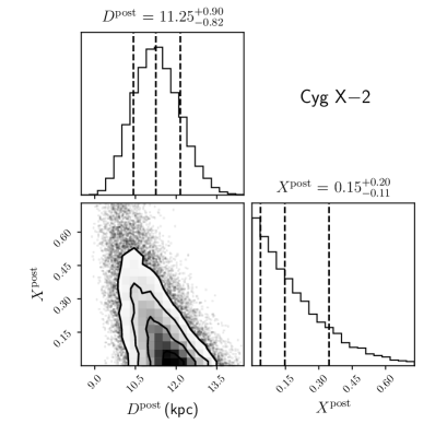 |
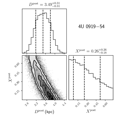 |
|
Refining nominal PRE distances and compositions of nuclear fuel
To better understand the statistical properties of (and to refine the PRE distance), we subsequently constrained both and the nominal PRE distance of each PRE burster with its calibrated parallax in a Bayesian way. The 2-D joint probability distribution (JPD) we applied is
| (5.4) |
where represents the Galactic prior term, i.e. the prior probability of finding a PRE burster at a distance along a given line of sight. We approached by the Galactic mass distribution of LMXBs, which can be calculated with Equation 5 of Atri19 using parameters provided by Grimm02; Atri19. Among the three components of the Galactic mass density (i.e. , and , see Grimm02 for explanations), the Galactic-disk component dominates the Galactic mass density budget for LMXBs at the light of sight to any of the three PRE bursters. Therefore, for this work alone, we adopted (see Equation 5 of Grimm02) as the Galactic prior term .
Following the JPD, we simulated posterior {, } pairs (hereafter referred to as and ), using bilby333https://lscsoft.docs.ligo.org/bilby/ (Ashton19). For this simulation, we adopted a uniform distribution between 0 and 0.73 for and a uniform distribution between 0 and 50 kpc for (where using a larger upper limit of does not change the result). Based on the marginalized probability density functions (PDFs) of the simulated {, } chain, we estimated and , which are presented in 5.2 and 5.4.
In general, the conversion of parallax to distance depends on the adopted Galactic prior (Bailer-Jones15). As an example, A21 found that the application of different Galactic priors (e.g. Bailer-Jones21; Atri19) results in inconsistent distances (see Figure 3 of A21). Unlike A21, we applied an extra constraint on provided by the PRE distance (see 5.4), which gives a handle on and improves the constraint on . With this extra constraint, the dependence on the Galactic prior becomes negligible for all of the three PRE bursters: their and stay almost the same without the term.
The PDFs of provide richer information on than . As expected from , the PDF of for Cen X4 favors a hydrogen-poor nature of nuclear fuel. In addition to the new constraint we put on , the nominal PRE distance of each PRE burster incorporating the parallax information is supposed to be more reliable (though not necessarily more precise). We note that the refined nominal PRE distances are still model-dependent; their accuracies are subject to the validity of the simplistic PRE model.
5.5.3 A roadmap for testing the simplistic PRE model with parallax measurements
The discussion in 5.5.2 is based on the correctness of the simplistic PRE model. Now we discuss the potential feasibility of using parallaxes (of PRE bursters) to test the simplistic PRE model. We first define the PRE distance correction factor () using the relation
| (5.5) |
where stands for the nominal PRE distance at (derived from the simplistic PRE model), and refers to the “true” distance. If the simplistic PRE model is correct, then . However, is possible due to various causes including the stochasticity of PRE burst luminosity and anisotropy of PRE burst emission (e.g. Sztajno87). The latter cause implies to be geometry-dependent (e.g. viewing-angle-related); if all PRE bursters have different geometry-dependent , a search for a global deviation of from unity with a sample of PRE bursters would be less practical. Nevertheless, it remains practical to constrain on an individual basis. One way to make this constraint is using the generalized , defined as
| (5.6) |
Accordingly, . Thanks to the same mathematical formalism, we can re-use 5.4 as the JPD for statistical analysis, except that the domain of is widened to .
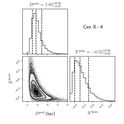 |
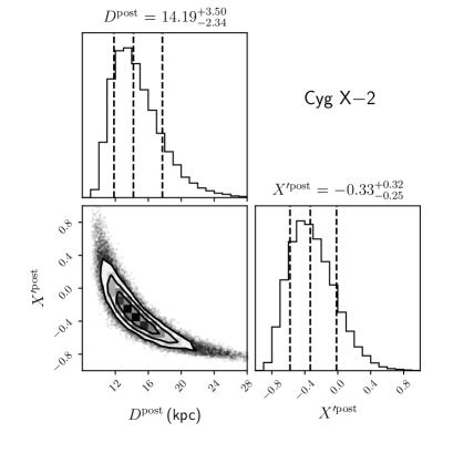 |
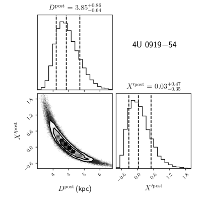 |
|
The simulated {, } chain (posterior and ) is depicted in 5.3. If the simplistic PRE model is correct, then ; as a result, is supposed to fall into the “standard” domain of [0, 0.73]. None of the three PDFs of decisively rules out from this standard domain. However, we notice at 90% confidence for Cen X4, which moderately disfavors the simplistic PRE model.
As the domain of is broadened from that of , the fractional precision of becomes predominantly reliant on that of the parallax. In this regime, and become more dependent on the adopted Galactic prior. To understand the degree of this dependence, we re-estimated and after resetting the Galactic prior to , which are summarized in 5.5. For Cyg X2 with insignificant , the dependence on the Galactic prior is evident, despite the consistency between the two sets of and . For Cen X4 and 4U 091954 both having relatively significant , the degree of the dependence varies with the Galactic coordinates of the targets. In particular, we found the and of Cen X4 are robust against the selection of Galactic priors in 5.4.
| PRE | ||||
|---|---|---|---|---|
| burster | (kpc) | (kpc) | ||
| Cen X4 | ||||
| Cyg X2 | ||||
| 4U 091954 |
Using as a probe of the simplistic PRE model has the advantage of being independent of the PDF for , which is usually not available. Future and measurements with higher precision will sharpen the above test of the simplistic PRE model. Lower fractional uncertainty of will not only reduce the strong correlation between and for Cyg X2 and 4U 091954 (shown in 5.3), but also lessen the dependence of inferred and on the adopted Galactic prior. On the other hand, constraining at PRE bursts independently (with, for example, ignition models of X-ray bursts) is the key to singling out . Given that the simplistic PRE model is not significantly disfavored by any of the 3 PRE bursters, the refined distances in 5.4 (based on the correctness of the simplistic PRE model) are still valid.
5.5.4 Future prospects
The potential of constraining and testing the simplistic PRE model using Gaia parallaxes of PRE bursters hinges on the achievable parallax uncertainties. Future Gaia data releases include Gaia Data Release 4 (DR4) (for the five-year data collection) and the data release after extended observations of up to 5.4 years (https://www.cosmos.esa.int/web/gaia/release). We predict the achievable parallax () and proper motion uncertainties of Cen X4 for future Gaia data releases using the simulation method detailed in the Appendix. In the same way, we estimated the predicted uncertainty of Cyg X2, 4U 091954 and XB 212947 for future data releases and DR2, which are listed in 5.6. The predicted uncertainties for DR2, denoted as , generally agree with the real values (see 5.6). In general, our simulation shows Gaia parallax and proper motion precision improves with observation time at roughly and , respectively.
| PRE | ∗ | ||||
|---|---|---|---|---|---|
| burster | (mas) | (mas) | (mas) | (mas ) | (mas) |
| Cen X4 | 0.16 | 0.15 | 0.13 | 0.10 | 0.07 |
| Cyg X2 | 0.024 | 0.024 | 0.019 | 0.014 | 0.010 |
| 4U 091954 | 0.08 | 0.07 | 0.06 | 0.05 | 0.03 |
| XB 212947 | 0.10 | 0.09 | 0.08 | 0.06 | 0.04 |
∗ we adopt an indicative 5-yr extension on top of the Gaia 5-yr mission.
According to 5.3, the future parallax uncertainty of Cyg X2 will be predominantly limited by the uncertainty of , or . For this target, improvement in the estimation of the zero-point parallax correction and its uncertainty – which is challenging due to the relative brightness of the source – is essential. In comparison, the of Cen X4, 4U 091954 and XB 212947 dominates the respective error budget of the calibrated parallax . Therefore, one can expect of Cen X4, 4U 091954 and XB 212947 to be potentially 1.9 times more precise (than EDR3) at the end of the extended Gaia mission (with 10-yr data), which would promise better constraints on and for Cen X4 and 4U 091954. On the other hand, to constrain and for XB 212947 with its already relatively precise Gaia parallax will require more PRE bursts to be detected from XB 212947. Apart from Gaia astrometry, radio observations of PRE bursters during their outbursts using very long baseline interferometry technique can also potentially measure geometric parallaxes of PRE bursters, hence serving the same scientific goals outlined in this paper.
This work only deals with the simplistic PRE model, the hitherto most impactful PRE model. As is mentioned in 5.2, PRE models are not the only pathway to the distances of type I X-ray bursters. Bayesian inference based on a burst ignition model (Cumming00) was recently realized to estimate parameters including and (Goodwin19). We believe such inferences will be made for more type I X-ray bursters in the near future. In Bayesian analysis based on burst ignition models (e.g. Cumming00; Woosley04), model-independent geometric parallaxes will serve as prior knowledge and help refine the inferred parameters including and ; the parallaxes can also judge which burst ignition model is more likely correct with a Bayes factor analysis.
Finally, we reiterate that we have assumed and km for all PRE bursters. Therefore, strictly speaking, should also reflect the deviation of and from their respective assumed values. Though a large deviation of from 1.4 is rare, it is not impossible (Shao20). In general, would increase with larger and (see 5.1). For example, is 40% greater than . Such a would correspond to assuming and the simplistic PRE model is correct. This value is consistent with for Cen X4. Given that the NS mass distribution is relatively well constrained compared to the NS radius distribution, it is possible to constrain the NS radius of a PRE burster in a Bayesian framework (slightly different from this work) provided prior knowledge of , and , assuming the simplistic PRE model is correct.
5.6 Conclusion
This work joins the few previous efforts to determine the Gaia parallax zero-point for a single source using nearby (on the sky) background quasars. We provide a new template for determination (which also includes the uncertainty) approached by the weighted standard deviation of quasar parallaxes with respect to the filter parameters (see 5.4). This work focuses on the small sample of PRE bursters with detected Gaia parallaxes . A future work will apply the new template to a larger sample of targets, which can enable a comprehensive comparison with zero-parallax points estimated in other ways.
We also introduce a Bayesian framework to test the simplistic PRE model with parallaxes of PRE bursters on an individual basis. Though no parallax of the PRE bursters decisively disfavours the simplistic PRE model, the model is disfavored by the current Cen X4 parallax at 90% confidence. At the end of the extended Gaia mission with 10-yr data, we expect the parallax precision to improve by a factor of 1.9, which will sharpen the test of the simplistic PRE model. This test will also considerably benefit from an independent determination of (hydrogen mass fraction of nuclear fuel), which we highly encourage.
Acknowledgements
The authors thank Ilya Mandel, Chris Flynn and Adelle Goodwin for useful discussions, and are grateful to the anonymous referee for the helpful comments on the manuscript. H.D. is supported by the ACAMAR (Australia-ChinA ConsortiuM for Astrophysical Research) scholarship, which is partly funded by the China Scholarship Council. A.T.D is the recipient of an ARC Future Fellowship (FT150100415). Parts of this research were conducted by the Australian Research Council Centre of Excellence for Gravitational Wave Discovery (OzGrav), through project number CE170100004. This work has made use of data from the European Space Agency (ESA) mission Gaia (https://www.cosmos.esa.int/gaia), processed by the Gaia Data Processing and Analysis Consortium (DPAC, https://www.cosmos.esa.int/web/gaia/dpac/consortium). Data analysis was partly performed on OzSTAR, the Swinburne-based supercomputer.
Appendix: Simulating the parallax precision of Cen X4 in future Gaia data releases
To simulate the uncalibrated parallax () precision of Cen X4 for a future Gaia data release, we made two assumptions: 1) Cen X4 is observed by Gaia at equal intervals; 2) , ( and ), where and stand for, respectively, the uncertainty of right ascension (RA) and declination at the -th observation.
The observation interval is determined with Table 1 of Gaia-Collaboration16. At the ecliptic latitude of Cen X4 (), the number of observations is 63 over 5 yr, corresponding to an interval of 29 d. It appears from 5.2 that, for a specific target, (where and represent uncertainty of and respectively), which implies the ratio of spatial resolution between RA and declination deviates slightly from unity and changes with pointing. Hence, we set to 1.21, which is the of Cen X4 from EDR3.
Simulated positions of Cen X4 were generated with pmpar (available at https://github.com/walterfb/pmpar) using the “predictor mode”, based on the astrometric parameters of Cen X4 in 5.2. We first simulated positions from MJD 56863 to MJD 57901 (the observing period of EDR3). The sole variable (and accordingly) was tuned to make the parallax precision equal to 0.13 mas, the current parallax precision of Cen X4. Subsequently, we stuck to the position uncertainties while extending the observing period to MJD 58689 (around the end day of the five-year period) and MJD 60516 (an indicative day 10 years after the first light of Gaia), which, respectively, yield parallax uncertainties of 0.095 mas and 0.067 mas. Thus, we predict the parallax precision of Cen X4 to improve by a factor of 1.3 and 1.9, respectively, with DR4 and 10-yr data. Besides, we expect the proper motion precision of Cen X4 to be enhanced by 2.7 and 6.7 times, respectively, with DR4 and 10-yr data.
Chapter 6 Probing Alternative Theories of Gravity with VLBI Astrometry of Pulsar-white-dwarf Systems
This chapter is converted from Ding20 and an erratum (Ding20d). Ding20, entitled “Very Long Baseline Astrometry of PSR J10125307 and its Implications on Alternative Theories of Gravity”, is the second publication (following Vigeland18) of the catalogue. This chapter and 7 focus on tests of gravitational theories in different regimes. 7 tests general relativity in the strong field regime using a double neutron star system, while this chapter constrains alternative theories of gravity with pulsar-white-dwarf systems that are potentially effective emitters of hypothetical dipole gravitational radiation (e.g. Eardley75). The astrometric inference of PSR J10125307 was revisited using Bayesian analysis in 8, as the Bayesian astrometric inference package sterne had not been developed by the publication of Ding20. In response to a minor comment by the thesis examiners, and at 95% confidence are added to 6.5.3.
6.1 Abstract
PSR J10125307, a millisecond pulsar in orbit with a helium white dwarf (WD), has been timed with high precision for about 25 years. One of the main objectives of this long-term timing is to use the large asymmetry in gravitational binding energy between the neutron star and the WD to test gravitational theories. Such tests, however, will be eventually limited by the accuracy of the distance to the pulsar. Here, we present VLBI (very long baseline interferometry) astrometry results spanning approximately 2.5 years for PSR J10125307, obtained with the Very Long Baseline Array as part of the project. These provide the first proper motion and absolute position for PSR J10125307 measured in a quasi-inertial reference frame. From the VLBI results, we measure a distance of kpc (all the estimates presented in the abstract are at 68% confidence) for PSR J10125307, which is the most precise obtained to date. Using the new distance, we improve the uncertainty of measurements of the unmodeled contributions to orbital period decay, which, combined with three other pulsars, places new constraints on the coupling constant for dipole gravitational radiation and the fractional time derivative of Newton’s gravitational constant in the local universe. As the uncertainties of the observed decays of orbital period for the four leading pulsar-WD systems become negligible in years, the uncertainties for and will be improved to and , respectively, predominantly limited by the distance uncertainties.
6.2 Introduction
6.2.1 Testing gravity theories with millisecond pulsars
When the beams of radiation emitted by rotating neutron stars (NSs) sweep across our line of sight, the result is a regular, lighthouse-like train of pulses. Thanks to their high rotational inertia, the spin period is extremely stable. The difference between observed pulse times of arrival (ToAs) and the model prediction for those ToAs is known as their residuals. The residuals are generally used to study unmodeled or imperfectly modeled physical process that would affect the ToAs (e.g. Lorimer12). Such processes include propagation through ionised material surrounding a binary companion (e.g. Lyutikov05) or through the interstellar medium (ISM; e.g. Lyne68; Bhat04) and gravitational phenomena.
Einstein’s theory of general relativity (GR) is the simplest possible form among a class of candidate gravitational theories. Some alternatives to general relativity suggest a time dependence of Newton’s gravitational constant , which in most cases also necessitates dipolar gravitational wave emission (Will93). There are several ways to test GR and constrain alternative theories of gravity with pulsars. Highly relativistic double neutron star systems (e.g. Damour92; Burgay03), pulsar-white dwarf binaries (e.g. Lazaridis09; Freire12; Antoniadis13; Zhu15) and triple stellar systems hosting pulsars (Archibald18) have probed different regions of phase space for deviations from the predictions of general relativity. Taken collectively, an ensemble of pulsars can be used as a Pulsar Timing Array (PTA) to search for spatially correlated ToA variations that would betray the presence of nanohertz gravitational wave, such as those generated by supermassive binary black holes (Detweiler79).
The pulsars used in these tests belong to a sub-group of pulsars called “recycled” or “millisecond” pulsars (MSPs). In this work, we use these two terms interchangeably to refer to pulsars spun up via accretion from a companion donor star (Alpar82). One of the reasons why MSPs are important for these experiments is that they exhibit less intrinsic timing noise compared to non-recycled pulsars (Shannon10), thus providing much better timing stability (e.g. Perera19) and higher timing precision; this is important for the detection of small relativistic effects in their orbits.
In addition to studies based on pulsar timing, Very Long Baseline Interferometry (VLBI) astrometric experiments are also carried out on both MSPs and normal pulsars (e.g. Chatterjee09; Deller16; Vigeland18; Deller19). By measuring annual geometric parallax and proper motion, VLBI astrometry can achieve model-independent estimates of distance, transverse velocity, and absolute positions for pulsars. It is significant not only in reducing the distance uncertainty and improving sensitivities of PTAs (Madison13), but also in various applications on a case by case basis.
6.2.2 The PSR J10125307 binary system
PSR J10125307 is a millisecond pulsar (MSP) with a 5.3 ms rotational period (Nicastro95). It has a helium white dwarf (WD) companion with mass (at 68% confidence level, as is any other quoted uncertainty in this paper unless otherwise stated, van-Kerkwijk96; Callanan98) in a 0.6-day-long (Lazaridis09) near-circular () orbit at a moderate inclination angle (Driebe98; Lange01). Spectroscopic observations of the WD were used to measure the mass ratio between PSR J10125307 and the WD companion to be by Callanan98 and by van-Kerkwijk04. A new spectroscopic study of PSR J10125307 by Mata-Sanchez20 further refines the mass ratio to . Antoniadis16 re-visited the Callanan98 data with an updated model for the helium WD, which resulted in an updated mass estimate of . In this paper, we will use the new mass ratio and WD mass , that corresponds to a mass estimate of 1.8 for the NS in PSR J10125307.
6.2.3 Motivations for improving the distance to PSR J10125307
The large difference in gravitational binding energy between the NS and WD in the PSR J10125307 system means that it would be an efficient emitter of dipolar gravitational waves in some alternate theories of gravity. Timing observations of such binary pulsars are able to offer experimental tests for those theories. Incorporating timing data from both PSR J10125307 and PSR J04374715, Lazaridis09 looked into the contributions to the time derivative of orbital period and use the difference between the modeled and observed value to constrain the coupling constant for dipole gravitational radiation to be and the fractional time derivative of Newton’s gravitational constant to be , both at 95% confidence. Using the same method but different pulsar-WD binaries, the best pulsar-based constraints, (at 68% confidence) and (at 95% confidence) are derived, respectively, by Freire12 and Zhu19.
For PSR J10125307 the precision of the constraints on and is dominated by the uncertainty in , and the distance to PSR J10125307 (Lazaridis09). Accordingly, improvements in the precision of distance estimates to pulsars such as PSR J10125307 have great potential to improve tests of alternate gravitational theories. Furthermore, as the uncertainty of decreases much faster than the uncertainty on the distance with pulsar-timing observations (Bell96), the latter will eventually dominate the error budget of and .
Improving the distance to PSR J10125307 will also benefit some other studies. Additionally, as one of the pulsars having reliable independent distance measurements, PSR J10125307 was used by Yao17 to derive the latest model of the Galactic free electron density distribution. Therefore a more accurate distance to PSR J10125307 would further refine such a model.
6.2.4 Measuring the distance to PSR J10125307
Several methods have been used in the past to estimate the distance to PSR J10125307, the results of which are summarized in 6.3. A measure of kpc was derived by Callanan98 using optical spectral-line observations of the WD companion. Pulsar timing is another way to measure the distance, as timing parallax is one of the outputs from parameter fits. PSR J10125307 is routinely timed by two PTAs, the European Pulsar Timing Array (EPTA) and the North American Nanohertz Observatory for Gravitational Waves (NANOGrav). To date, two timing parallaxes have been reported for PSR J10125307 utilizing solely EPTA data. Lazaridis09 reported a timing parallax of mas using 15 years of multi-telescope data, corresponding to a distance of kpc. A different timing parallax for PSR J10125307 mas is reached more recently in Desvignes16, showing tension with the previous timing result. The EPTA and NANOGrav data for PSR J10125307 are also combined and analysed collectively under the International Pulsar Timing Array (IPTA) collaboration, leading to a distance estimate kpc for PSR J10125307 (Verbiest16).
Apart from the above-mentioned methods, high-resolution trigonometric astrometry with VLBI or optical observations are able to provide model-independent distance estimation. A reliable distance to PSR J10125307 is essential for improving the uncertainty of and dipole gravitational wave emission (see 6.5.3 for explanation). As well as GR tests, a distance based on trigonometric parallax reinforces the estimation of the bolometric luminosity of the companion WD, which reveals the WD radius. The WD radius can be translated to the WD mass when the mass-radius relation is worked out. Incorporating the known NS-WD mass ratio (Mata-Sanchez20), we can estimate the NS mass.
Prior to this work, an optical counterpart for PSR J10125307 has been identified by Jennings18 in the Gaia second data release (DR2) (Gaia-Collaboration16; Gaia-Collaboration18), carrying a tentative parallax of mas. The parallax was then translated into a Gaia distance kpc for PSR J10125307 incorporating other prior information (Jennings18). In this work we focus on VLBI astrometry of PSR J10125307 as part of the project, which is the extension of project (Deller16; Vigeland18; Deller19) focusing exclusively on MSPs. Throughout this paper, parameter uncertainties are quoted to 68% confidence level unless stated otherwise.
6.3 Observations and data reduction
PSR J10125307 was observed at L band (central frequency 1550 MHz) with the Very Long Baseline Array (VLBA) in eight epochs between July 2015 and November 2017 under the observation codes BD179 and BD192. Each session was 1 h long, and the observations are summarized in 6.1. The observational setup is in general the same as other pulsars in and sample (refer to Deller19), while using J09585039 as phase reference calibrator and J11181234 to calibrate the instrumental bandpass. Four compact extragalactic radio sources within 9 arcminutes of PSR J10125307 were identified as suitable in-beam calibrators in early observations, from which J101307.3531234 is chosen as the primary in-beam calibrator due to its relative brightness (6.2). The data were correlated using the DiFX software correlator (Deller11a) in two passes - gated and ungated. After gating, the S/N increases by %. The gated visibility datasets are subsequently processed in a python-based ParselTongue (Kettenis06) pipeline calling AIPS (Greisen03) and DIFMAP (Shepherd94) functions, described in Deller19. The reduction pipeline is publicly available now at https://github.com/dingswin/psrvlbireduce. It is to be released incorporating better readability, configurability, some new functions and extended diagnostic tools. The data for PSR J10125307 were reduced using the pipeline versioned a6b666e. Multiple runs of the pipeline are made to iteratively flag bad visibility data (e.g., due to radio frequency interference), make uniform models for calibrators (including the phase calibrator, fringe finder and in-beam calibrators) and obtain reliable positions for PSR J10125307.
| yyyy-mm-dd | Project | S/N | RA | Dec |
|---|---|---|---|---|
| Code | (J2000) | (J2000) | ||
| 2015-07-16 | bd179e0 | 58.9 | 53∘07’0214401(916) | |
| 2015-11-15 | bd179e1 | 96.8 | 53∘07’0213524(616) | |
| 2016-11-11 | bd192e0 | 87.7 | 53∘07’0211042(616) | |
| 2016-11-19 | bd192e1 | 85.0 | 53∘07’0210984(820) | |
| 2017-05-10 | bd192e2 | 88.2 | 53∘07’0209865(719) | |
| 2017-05-29 | bd192e3 | 46.8 | 53∘07’0209682(1219) | |
| 2017-06-11 | bd192e4 | 31.0 | 53∘07’0209639(1923) | |
| 2017-11-26 | bd192e5 | 17.9 | 53∘07’0208382(3438) |
| Source | Name in data | Purpose | |
|---|---|---|---|
| PSR J10125307 | J10125307 | 0 | target |
| J11181234 | J11181234 | 426 | fringe finder/bandpass calibrator |
| J09585039 | J09585039 | 326 | phase calibrator |
| J101307.3531234 | IBC00462 | 751 | primary in-beam calibrator |
| J101307.4530423 | IBC00412 | 574 | in-beam calibrator |
| J101230.6525826 | IBC00421 | 862 | in-beam calibrator |
| J101204.0531332 | IBC00460 | 785 | in-beam calibrator |
6.4 Systematic errors and parallax fits
After data reduction, we determined positions of PSR J10125307 at eight epochs, which are summarized in 6.1. The statistical positional uncertainties obtained from an image-plane fit are reported to the left of the ”” symbol in 6.1. However, we expect a significant contribution from systematic position shifts, and the uncertainties in 6.1 to the right of ”” symbol incorporate both the statistical uncertainty already mentioned and an empirical estimate of systematic uncertainty. This estimate is made using the following empirical function rewritten from Deller19:
| (6.1) |
where is the ratio of the systematic error to the synthesized beam size, stands for elevation angle, is the average for a given observation (over time and antennas), is the angular separation in arcmin between J101307.3531234 and PSR J10125307, represents the signal-to-noise ratio of J101307.3531234, and and are empirically determined coefficients based on the sample. The first term in 6.1 represents propagation-related systematic errors, while the second term accounts for random errors resulting from the calibration solutions from the primary in-beam calibrator. In general, propagation-related systematic errors (proportional to the separation between calibrator and target) dominate the systematic (and indeed overall) error budget. This is still true in this work, even if the first term is significantly reduced by the usage of in-beam calibrators.
For PSR J10125307, the contribution from the first term is 3 times that of the second term. The full uncertainties are the addition in quadrature of statistical and systematic uncertainties. The inclusion of systematic uncertainties decreases the of least-squares astrometric fit from 7.9 to 1.9, which indicates that the uncertainty estimation is likely reasonable (although perhaps still modestly underestimated).
6.4.1 Astrometric fitting
We used pmpar111https://github.com/walterfb/pmpar to perform astrometric fitting for parallax, proper motion and reference position. As found by Deller19 for PSR B191316, using a bootstrap technique to estimate the astrometric parameters was consistent with but more conservative than a least-squares fit, and we followed this approach for PSR J10125307. We bootstrapped 130000 times from the 8 positions with full uncertainties (i.e., in every run we drew positions eight times with replacement from the set of positions and performed astrometric fitting on the drawn sample) for estimation of the astrometric parameters. It is possible that the eight draws contain fewer than three effective epochs, which is the minimum required for astrometric fitting. In order to limit the number of severely biased fits yielded by overly short time baselines or negligible variation in the contribution of parallax between epochs, we required at least 4 effective epochs for subsequent fitting in every bootstrap run. 6.1 shows the stacked position evolution removing best fitted proper motion. Each line is the fitting result out of one bootstrap run. The densest part corresponds to the estimated parallax, position and proper motion. Using the probability density functions of parallax and proper motion obtained from the bootstrap runs (see 6.2), we determined the measured value and corresponding uncertainty, which are summarized in 6.3 along with the results of a simple linear least squares fit. For each astrometric observable (i.e. parallax, proper motion, or reference position), its measured value corresponds to the peak of its probability density function; its uncertainty is given by the narrowest interval that encloses 68.3% of its 130000 bootstrapped results.
As is seen in 6.3, the uncertainties from bootstrap are much more conservative than direct fitting, and are possibly over-estimated since the for direct fitting is already close to unity. We use the bootstrap results in the following discussions. The histogram for is bimodal in 6.2, which is discussed in 6.5.1. Lutz-Kelker correction was not carried out since our significance of parallax is well over the critical value between 5.0 and 6.7, indicating a negligible Lutz-Kelker effect (Lutz73).
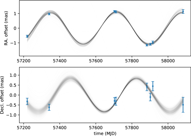
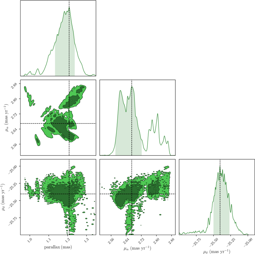
| method | references a | |||||
|---|---|---|---|---|---|---|
| (mas) | () | () | (kpc) | () | ||
| direct fitting | This work | |||||
| bootstrap | This work | |||||
| timing parallax (EPTA/2009) | b | (1) | ||||
| timing parallax (EPTA/2016) | c | (2) | ||||
| orbital parallax (EPTA/2016) | d | (2) | ||||
| timing (IPTA) | (3) | |||||
| timing (NANOGrav) | e | (4) | ||||
| Gaia DR2 | (5, 6, 7) | |||||
| spectroscopy | (8) |
a (1) Lazaridis09, (2) Desvignes16, (3) Verbiest16, (4) Arzoumanian18, (5) Gaia-Collaboration16, (6) Gaia-Collaboration18, (7) Jennings18, (8) Callanan98.
b Here, we have re-calculated using the parallax-based distance, rather than weighted distance for consistency (Lazaridis09).
c : Lutz-Kelker correction not applied for consistency.
d , distance derived from the (time derivative of orbital period) budget in GR regime.
e Classified by Arzoumanian18 as non-detection.
6.4.2 Absolute position for PSR J10125307
Absolute positions are of significance for comparing positions based on different reference frames. The position for PSR J10125307 that we obtain from bootstrapping is anchored to J101307.3531234, the primary in-beam calibrator. However, the absolute position of J101307.3531234 is not well determined, and we must estimate its position and uncertainty based on the observations. In order to derive the absolute position for PSR J10125307, we used J101307.3531234 to tie PSR J10125307 to J09585039. We used two methods to make this connection. In the first approach the calibration solutions derived by J09585039 were transferred to J101307.3531234, which was subsequently divided by the uniform J101307.3531234 model obtained from eight epochs; the centroid of the divided J101307.3531234 was located for each epoch; the average and scatter of the eight J101307.3531234 positions thus offer the information of the “real” J101307.3531234 position relative to J09585039 and the systematic uncertainty of this position. The second way is in principle the same while in the reverse direction: the final solution derived by J101307.3531234 was applied to J09585039. 6.3 shows the eight J101307.3531234 and J09585039 positions obtained in the two different ways. As is expected, from 6.3 we can conclude that 1) no time-dependence of position shifts is noticeable; 2) the scatter among the positions for the two objects, indicating the systematic errors around the mean position, is consistent in both RA and Dec. In each way we used the average position to tie J09585039 and J101307.3531234, thus anchoring PSR J10125307 to J09585039. The absolute positions derived from two ways are highly consistent; we proceed with their average position. Finally, we aligned PSR J10125307 to the latest J09585039 position222http://astrogeo.org/vlbi/solutions/rfc_2019a/rfc_2019a_cat.html, which is measured at higher radio frequencies based primarily on dual-band 2.3/8.4 GHz observations (Petrov08).
As the jet core of J09585039 is presumably the brightest spot in the J09585039 map, it is taken as the reference position for J09585039 after fringe fitting in AIPS. Since the jet core moves upstream towards the central engine with increasing frequency (e.g. Bartel86; Lobanov98), our presented absolute position is referenced to the jet core of J09585039 at L band, where its absolute position has not been determined. Sokolovsky11 compiled multi-band observations on 20 AGNs and reported the median core shift between X band and L band is 1.15 mas. A recent work by Plavin19 integrates long-term observations of 40 AGNs and concludes the core shift of AGNs between 8 GHz and 2 GHz is typically 0.5 mas. They additionally found time variability of core shift at an average level of 0.3 mas in 33 AGNs of the sample. With limited knowledge about the core shift of J09585039, we split the median core shift 1.15 mas evenly between the two axes and add them in quadrature to the errors of the absolute position of PSR J10125307.
The absolute position we obtained for PSR J10125307 is shown in 6.4. We chose the midpoint of the eight VLBI epochs as the reference time for astrometric fitting to obtain the highest precision for the absolute position of PSR J10125307, and note that extrapolating the position to earlier or later times will suffer progressively from the accumulation of proper motion uncertainty.
The uncertainty of the absolute position of PSR J10125307 comprises the bootstrap uncertainty of J09585039 position anchored to J101307.3531234 (i.e. the uncertainty derived from the normalized histogram of RAs/Decs as shown in 6.2), the systematic errors in J09585039J101307.3531234 connection (the scatter of eight positions) and the uncertainty of the absolute position of J09585039. These components are added in quadrature. In order to make comparison to timing results, we also extrapolated the timing positions for PSR J10125307 to our reference epoch MJD 57700 using the ephemerides of Lazaridis09; Desvignes16; Arzoumanian18 (see 6.4). Furthermore, we re-identified Gaia DR2 851610861391010944 as the optical counterpart for PSR J10125307: its predicted position at MJD 57700 is mas from our VLBI position (as shown in 6.4), while its proper motion and parallax are largely consistent with both the VLBI and timing results (6.3). The uncertainties of the timing and Gaia positions are estimated with Monte-Carlo simulation, assuming the astrometric parameters offered in literature (also reproduced in 6.3) follow a gaussian distribution.
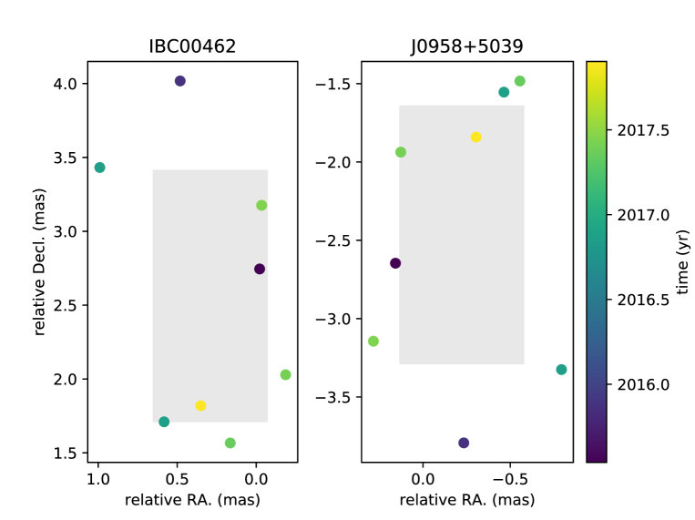
| This work | Lazaridis09 | Desvignes16 | Arzoumanian18 | Gaia DR2 | |
|---|---|---|---|---|---|
| RA | a | b | |||
| Dec. | 53∘07’02113(1) | 53∘07’021094(4) | 53∘07’021113(1) | 53∘07’0211090(9) | 53∘07’021098(9) |
aThe uncertainty for both R.A. or declination includes an estimate of the systematic error introduced by core shift in the reference source between 1.5 GHz and 8.4 GHz, taken as 0.8 mas in each axis as described in the text.
bGaia-Collaboration16; Gaia-Collaboration18; Jennings18
6.5 Discussion
6.5.1 Comparison to timing astrometry
There are two published parallaxes and three proper motions for PSR J10125307 based on timing astrometry (Lazaridis09; Desvignes16; Arzoumanian18). The timing proper motions disagree significantly, as shown in 6.3, indicating that the uncertainties have historically been somewhat underestimated. At the time of writing, the EPTA is the only PTA that detects a timing parallax for PSR J10125307 (Lazaridis09; Desvignes16). Given the additional data available to the 2016 work, we would expect this to be the more accurate of the two EPTA results. Our proper motion and reference position agree with both EPTA measurements, slightly favoring the 2016 measurement. Our measured parallax, on the other hand, agrees with the 2009 measurement but is in significant tension () to the 2016 result. 6.3 shows that the Desvignes16 result is also inconsistent with other independently derived distance measurements, but the cause of the discrepancy is unknown.
When we consider the VLBI results for proper motion, a bimodality is apparent in the probability density obtained for in 6.2. The sub-peak of at 2.8 is strongly disfavored by all timing results (cf. 6.3). We diagnosed the origin of this bimodality by removing one epoch at a time from our bootstrap procedure and found that the inclusion of the second epoch (BD179E1) is responsible for the sub-peak of the histogram. However, since there is no clear evidence of a bad measurement at the second epoch (cf. 6.1), we did not take any action such as removing this observation. The availability of pulsar timing proper motions does, however, offer the opportunity to study the effect of applying prior information when conducting the VLBI fitting.
VLBI astrometry is performed in a quasi-inertial reference frame, determined by numerous distant AGNs whose positions (as determined by VLBI observations) are assumed to be fixed. Examples of realizations of such a reference frame include the International Celestial Reference Frame version 3 (ICRF3333www.iers.org/IERS/EN/DataProducts/ICRF/ICRF3/icrf3.html) and the Radio Fundamental Catalog (RFC444astrogeo.org/rfc/). Timing astrometry, on the other hand, is performed after referencing the pulse ToAs to the barycenter of the solar system, making use of a solar system ephemeris (SSE). Due to the different nature of the reference frames used by VLBI and timing astrometry, a small-scale 3-dimensional rotation between the two types of reference frames is possible, and this rotation could be time-dependent. As a result, small differences in the reference position might be seen between quantities measured using VLBI versus those measured using pulsar timing. Unless the time dependence of the frame misalignment was extremely large, however, the effect on proper motion and (especially) parallax would be extremely small compared to current levels of precision.
The 3-dimensional transformation between ICRF and barycentric frame can be decomposed into a 2-d translation and a 1-d rotation as the displacement is only mas level (Wang17). This can be visualized as the translation and rotation of a local 2-d frame in its surface. The proper motions obtained from VLBI and timing astrometry differ only when there is a noticeable 1-d frame rotation. Under the safe assumption that the angle of the 1-d frame rotation is smaller than 1 arcmin, the effect of frame transformation on proper motion would be insignificant, and we can in principle make use of the timing proper motions as priors to the VLBI astrometric fitting. The longer time baseline of timing observations promises better precision of proper motion. Therefore if the assumption is met, the application of timing proper motion would potentially improve our parallax estimation.
We fixed to the 2009, 2016 and 2018 respectively (see 6.3) and ran bootstrapping again. The resultant parallax probability density functions are shown in 6.4. The peak of the normalized histogram of parallax changes slightly with , as a result of the correlation between parallax and (shown by the corresponding error “ellipse” in 6.2). In all cases, the effect of applying the timing proper motion prior is to reduce the most probable parallax value by a small fraction of a standard deviation, and for the most recent timing proper motion results (Desvignes16; Arzoumanian18) the overall parallax uncertainty is reduced.
However, the timing measurements of disagree by much more than their formal uncertainties, making it difficult to select the most accurate to impose as a prior. Therefore, for simplicity and self-consistency, we use the VLBI results obtained with no priors from the timing proper motion as shown in 6.3 in following discussion, but note that 1) the application of a well-motivated prior based on timing could further improve the VLBI parallax and hence distance precision, and 2) whichever timing proper motion is chosen, the effect is to reduce the VLBI parallax and hence increase the estimated distance to the pulsar.
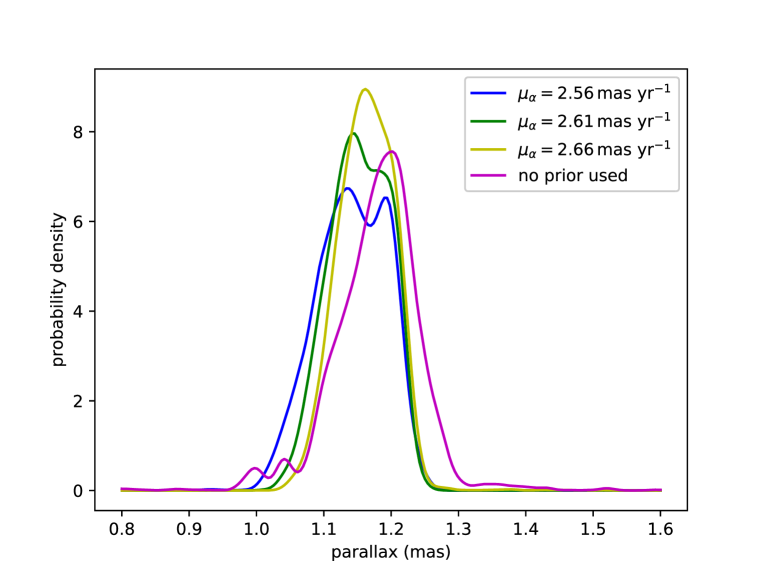
6.5.2 Galactic path from updated 3D velocity
The orbit of PSR J10125307 through the Galaxy was determined by Lazaridis09, who used their best-fit proper motion and distance along with a radial velocity of estimated by Callanan98. Tracing it back for 10 Gyr in a model for the Galactic potential they found that it is only rarely passes close to the Sun; rather it spends more time out at Galacto-centric distances of 30 kpc and oscillating vertically up to 7 kpc above/below the Galactic plane. However, Freire11 used the same data to find different conclusions. The Galacto-centric distances range from 4 kpc to 7 kpc, and the vertical oscillations go to 2 kpc above/below the Galactic plane.
With our new distance as well as the improved radial velocity (Mata-Sanchez20), we can once again repeat this exercise. We use the MWPotential2014 potential from galpy (Bovy15) for tracing the orbit of the pulsar. In contrast to Lazaridis09 and similar to Freire11, rather than spending little time near the Sun and orbiting out to 30 kpc, we find that PSR J10125307 orbits largely within the Solar circle, going from Galactocentric radii of 3.5–8.5 kpc on a timescale of Myr. Similarly, rather than oscillating to kpc in the vertical direction it only moves to kpc (the difference between our results and those of Freire11 are largely due to the different value of that we assumed). These results are robust to the choice of potential: using the same analytic potentials as Lazaridis09 gives essentially the same overall orbits. This is not surprising, as the 3D space velocity of PSR J10125307 of relative to the Local Standard of Rest (based on the Solar motion of Schonrich10) is largely consistent with the MSP distribution (Matthews16), or maybe a little high, and the current vertical location in the Galaxy pc is likewise consistent with the MSP distribution (Ng14), suggesting a vertical orbit that mimics the overall MSP population with a vertical scale height of kpc.
6.5.3 Constraints on and dipole gravitational radiation
Since Lazaridis09 constrained alternative theories of gravity using timing analysis on PSR J10125307, timing parameters including (the observed time derivative of orbital period) have been updated by Desvignes16. Despite the probable biased parallax presented by the 2016 work (as discussed in 6.5.1), improved measurements for a number of other parameters are expected as a result of longer observation time, most notably (for our purposes) the orbital period derivative and proper motion. The reported by Desvignes16 is consistent with the 2009 counterpart , but is 3 times more precise. The accuracy of reported by Desvignes16 is dominated by the precision of .
Besides the improved timing precision, the companion mass and mass ratio of PSR J10125307 are also better constrained to (Antoniadis16) and (Mata-Sanchez20) respectively. These, along with our new parallax, allows us to improve the constraints on the (time derivative of Newton’s gravitational constant) and dipole gravitational radiation. The method we adopt here has been developed by Damour88; Nordtvedt90; Damour91; Lazaridis09; Freire12; Zhu15.
Contributions to the time variation of orbital period of PSR J10125307 can be summarized as
| (6.2) |
where and are not intrinsic to the PSR J10125307 binary, representing the effect of radial acceleration of PSR J10125307 induced by Galactic gravitational potential (Damour91; Nice95) and transverse motion (Shklovskii70), respectively; , and are contributions intrinsic to the binary system resulting from gravitational-wave damping, mass loss of the binary (Damour91; Freire12) and a deformed companion (Smarr76; Freire12), respectively; stands for excess term of non-GR origins. As the non-intrinsic terms of are dependent on distance and proper motion, we are able to refine and with our new astrometric results.
The Shklovskii term can be calculated with
| (6.3) |
where , is the distance of PSR J10125307 from the Sun and is the speed of light. For the convenience of error propagation, the larger side of uncertainties for parallax and proper motion (6.3) are used as their symmetric uncertainties in the following calculation, i.e. mas, , . Our new parallax and proper motion render , the uncertainty of which is 63% of the counterpart in Lazaridis09. In the same way as Zhu15 (and references therein), we updated with our new parallax-based distance to PSR J10125307, taking the Sun-GC (Galactic Center) distance to be kpc (Gravity-Collaboration18) and circular speed of the local standard of rest to be (McGaugh18). Combining the new mass ratio (Mata-Sanchez20) into Equation (21) from Lazaridis09, we acquire , where the uncertainty is dominated by the WD mass.
These updated contributions of , along with negligible and (Lazaridis09), give , 2.6 times more precise than the counterpart in Lazaridis09. The contributions to as well as the derived for our work and Lazaridis09 are summarized in 6.5.
| This work | 61(4) a | 68.6(4.4) | -5.5(2) | -13(1) | 0 | 0 | 10.6(6.1) |
| Lazaridis09 | 50(14) | 70(7) | -5.6(2) | -11(2) | 0 | 0 | -4(16) |
aDesvignes16
As already noted, some alternative theories of gravity demand dipole gravitational radiation and/or a time-dependence to Newton’s gravitational constant in the local universe. The new , consistent with zero at 1.7 confidence level, does not support alternative theories to GR. Nevertheless, we can make use of this measurement to set new limits to dipole gravitational radiation and with
| (6.4) |
where and represent orbital change caused by and dipole gravitational radiation, respectively. The relation between and is rewritten from Damour88; Nordtvedt90; Lazaridis09 as
| (6.5) |
where (Mata-Sanchez20) is the mass ratio between the pulsar and the companion, stands for the “sensitivity” of the pulsar depending on its EoS, mass and the theory of gravity in concern (Will93). The connection between and , the putative coupling constant of dipole gravitational radiation, is reproduced from Lazaridis09 as
| (6.6) |
where s, (Antoniadis16) is the mass of the companion. Here we assume the higher-order terms of the “sensitivities” of the pulsar and the companion are negligible.
There are two ways to solve and from 6.4, 6.5, 6.6. They are both based on the universality of physical laws, i.e. and do not vary in the local universe. The first method is borrowing independent or from other measurements. The second one is using several well timed pulsars to solve or fit (when using more than 2 pulsars) and at the same time, introduced by Lazaridis09.
To date, the most stringent limits on are provided by lunar laser ranging (LLR), which yields (95% confidence level Hofmann18), and modelling of the orbit of Mercury , which yields (95% confidence level Genova18). The from LLR can be translated into , thus assisting us to gauge separately. We use the LLR constraint in preference to that from Genova18 due to the ambiguity of the sign of the latter. In order to solve in 6.6, we assume ) (where ), as proposed by Damour92a and adopted by Lazaridis09; Zhu15. We hence obtain and . The latter gives (95% confidence level), which is 3.6 times as precise as the previous effort with PSR J10125307 made utilising the same approach (Lazaridis09). This estimate of is, however, less precise than the (68% confidence level) by Freire12 acquired with the same method while using PSR J17380333.
As the second way to solve and , we combined PSR J10125307 with PSR J04374715, PSR J17380333 and PSR J17130747 to extract and , following the method introduced by Lazaridis09. The three other pulsars have been used to constrain and (Verbiest08; Deller08; Freire12; Zhu19). The parameters of the four pulsars we used to derive and are summarized in 6.6. We approach and by least-square fitting, and their uncertainties by Monte-Carlo simulation. The marginalized and we obtain are
| (6.7) |
| (6.8) |
at 68% confidence, and
| (6.9) |
| (6.10) |
at 95% confidence. These values are consistent with zero, and comparably precise to (and more conservative than) and measured at 95% confidence by Zhu19. We note that we have adopted the relation ), and hence these two estimates are dependent on this assumed relation. The mathematical formalism of hinges further on the EoS of NSs, which will be better constrained by NICER (Bogdanov19; Bogdanov19a) and the gravitational-wave observatories (Annala18) in the years to come.
| pulsar | references | |||||
|---|---|---|---|---|---|---|
| d | ||||||
| PSR J04374715 | 5.74 | 12(32) a | 1.44(7) | 0.224(7) | Reardon16; Deller08 | |
| PSR J10125307 (this work) | 0.60 | 10.6(6.1) | 0.174(11) | 10.44(11) | references in this paper | |
| PSR J17130747 | 67.83 | 30(150) | 1.33(10) | 0.290(11) | Zhu19 | |
| PSR J17380333 | 0.35 | 2.0(3.7) | 1.46(6) | 8.1(2) | Freire12 |
aWe derived for PSR J04374715 with the results from Reardon16; Deller08.
6.6 Conclusions and future prospects
-
1.
This paper reports new VLBI astrometry of PSR J10125307 (6.3). Our new distance to PSR J10125307, kpc, is the most precise to date and consistent with major measurements. We present the first VLBI-based absolute position for PSR J10125307, which paves the road for the frame link between the quasi-static International Celestial Reference Frame used by VLBI and the solar-system frame used by pulsar timing.
-
2.
Using our new distance and proper motion, we reduce the uncertainty of the Shklovskii term in 6.2. On top of that, we set new constraints on the fractional time derivative of the Newton’s gravitational constant for the local universe and the coupling constant for dipolar gravitational radiation , combining three other millisecond pulsars, PSR J04374715, PSR J17380333 and PSR J17130747. The new is comparable to the most stringent constraint.
-
3.
As is shown in 6.6, among the four pulsars, the of PSR J10125307 stands out with offset from zero, which effectively brings the best-fit away from zero. If we only use the other three pulsars and re-do the analysis, we obtain , where the uncertainty increases but the best-fit becomes more consistent with zero. Therefore, whether of PSR J10125307 will converge to zero with future timing and VLBI observations of PSR J10125307 is essential for the test using pulsar-WD binaries. Assuming GR is correct, the 1.7 offset of from zero implies that the value of either our VLBI parallax and/or is too high (given that the other contributing terms of vary marginally). This mild tension will be re-visited with a better based on longer timing observations. As noted in 6.5.1, we see that applying constraints to the proper motion of PSR J10125307 based on pulsar timing act to reduce the VLBI parallax, albeit within the current uncertainties, which would already mitigate the tension somewhat. It is likely that the timing proper motions of PSR J10125307 acquired independently with EPTA and NANOGrav will converge to a value with negligible uncertainty in the future, allowing us to confidently apply this as a prior to our VLBI fit and improve our parallax estimate for PSR J10125307. Furthermore, when the uncertainties of both and the distance to PSR J10125307 are improved by a factor of 4 with new timing and VLBI observations, we are able to estimate the next uncertainty contributor to - the WD mass (as well as the pulsar mass), assuming . This independent WD mass will help refine the relation between WD mass and WD atmospheric parameters in the helium-WD regime.
-
4.
Looking into the future, the uncertainty of for PSR J10125307 will quickly vanish (as , Bell96), reducing the uncertainty of to in years. At that time, the Shklovskii term would become the leading error source of for PSR J10125307. Inside the Shklovskii term, the distance (or parallax) dominates the error budget as the uncertainty of parallax improves as . That means distance uncertainty will eventually become the biggest barrier against better constraints on alternative theories of gravity. This will be the same for the analysis of most555For some systems, especially PSR J17380333, the relatively low precision on the mass measurements - not the uncertainty on the distance - will be the main barrier towards improvement of the test. other MSPs. If we reduce the uncertainty of to zero for each of the four above-mentioned pulsars (PSR J10125307, PSR J04374715, PSR J17380333 and PSR J17130747) and re-derive and , we find the uncertainty reduces to for and for . This simulation shows significantly better constraints on and can be made with continuous efforts on pulsar timing for years. Beyond that, in order to further this study, we need to focus on improving the precision of distances to the pulsars of use.
Acknowledgements
HD is supported by the ACAMAR (Australia-ChinA ConsortiuM for Astrophysical Research) scholarship, which is partly funded by the China Scholarship Council (CSC). DLK and TJWL were supported by the NANOGrav Physics Frontiers Center, which is supported by the National Science Foundation award 1430284. Part of this research was carried out at the Jet Propulsion Laboratory, California Institute of Technology, under a contract with the National Aeronautics and Space Administration. The authors thank Norbert Wex and the anonymous referee for their important comments on this paper. The data of this work come from the Very Long Baseline Array (VLBA), which is operated by the National Radio Astronomy Observatory (NRAO). The NRAO is a facility of the National Science Foundation operated under cooperative agreement by Associated Universities, Inc. This work made use of the Swinburne University of Technology software correlator, developed as part of the Australian Major National Research Facilities Programme and operated under license.
Softwares
DiFX (Deller11a), ParselTongue (Kettenis06), AIPS (Greisen03), DIFMAP (Shepherd94), psrvlbireduce (https://github.com/dingswin/psrvlbireduce), pmpar (https://github.com/walterfb/pmpar)
Chapter 7 The Orbital-decay Test of General Relativity
with VLBI
Astrometry of the Second
Discovered Double Neutron Star
.
This chapter is adapted from Ding21a entitled “The Orbital-decay Test of General Relativity to the 2% Level with 6 yr VLBA Astrometry of the Double Neutron Star PSR J1537+1155”, which is the third paper (following Vigeland18; Ding20), and the only paper that tests general relativity in the strong field regime. This chapter marks the first time that the Bayesian astrometric inference package sterne was used in this thesis. However, the Bayesian inference does not yet include the systematics-correcting parameter to be introduced in 8.
As is pointed out in 8, the Galactic-potential-induced orbital-decay term (see 7.5) is not correctly estimated due to a coding error. As a result, the ratio between the observed orbital decay and the theoretical prediction is changed by a small but important fraction (1.8%). The corrected values of and are presented in 8.
7.1 Abstract
PSR J15371155, also known as PSR B153412, is the second discovered double neutron star (DNS) binary. More than 20 years of timing observations of PSR J15371155 have offered some of the most precise tests of general relativity (GR) in the strong-field regime. As one of these tests, the gravitational-wave emission predicted by GR has been probed with the significant orbital decay () of PSR J15371155. However, compared to most GR tests provided with the post-Keplerian parameters, the orbital-decay test was lagging behind in terms of both precision and consistency with GR, limited by the uncertain distance of PSR J15371155. With an astrometric campaign spanning 6 years using the Very Long Baseline Array, we measured an annual geometric parallax of mas for PSR J15371155, corresponding to a distance of kpc. This is the most tightly-constrained model-independent distance achieved for a DNS to date. After obtaining (i.e., the orbital decay caused by Galactic gravitational potential) with a combination of 4 Galactic mass distribution models, we updated the ratio of the observed intrinsic orbital decay to the GR prediction to , three times more precise than the previous orbital-decay test () made with PSR J15371155.
7.2 Introduction
7.2.1 Pulsars in double neutron star systems
Double neutron stars (DNSs) are prized testbeds on which to evaluate theories of gravity and to probe the composition of neutron stars (NSs). The DNS merger event GW170817 has been recorded both by gravitational-wave (GW) observatories and electromagnetically (e.g. Abbott17; Abbott17a; Goldstein17; Mooley18), providing constraints on the interior composition of NSs (e.g. Annala18). The same merger event also strengthens the belief that short Gamma Ray Bursts (SGRBs) are generated by DNS mergers (e.g. Coward12), though most SGRBs are well beyond the horizon of the current ground-based GW detectors. In addition, DNS mergers are considered the prime sources of r-process elements (Eichler89; Korobkin12; Drout17). To test the connection between DNS mergers and the observed abundance of r-process elements in the local universe, an estimate of the DNS merger rate is required, which can be constrained with observations of the Galactic DNS population (e.g. Kim15; Pol19).
During their steady inspiral stage, DNS systems can be studied by measuring and modeling the pulse time-of-arrivals (ToAs) from a pulsar residing in a DNS system (hereafter referred to as a “DNS pulsar”). So far, 16 known DNS pulsars and 3 suspected ones have been discovered from pulsar surveys (see Table 1 of Andrews19), including two found in globular clusters. Though in shallower gravitational potentials compared to DNS mergers, DNS pulsars provide some of the most precise tests on gravitational theories in the strong-field regime with long-term timing observations (e.g. Stairs03; Kramer06; Deller09). Gravitational theories are tested with DNS pulsars by comparing observed post-Keplerian (PK) parameters, which quantify effects beyond a simple Keplerian model of motion, to the predictions of a specific gravitational theory, e.g., the general theory of relativity (GR). However, the theory-dependent prediction of each PK parameters relies on the masses of the two DNS constituents. Therefore, one needs at least three PK measurements to test a gravitational theory, as two of them have to be used to determine the two DNS constituent masses (based on the theory to be tested). The PK parameters include (but are not limited to) , , , and , which stand for, respectively, the orbital decay, the advance of periastron longitude, the Doppler coefficient, the “range” of the Shapiro delay effect and the “shape” of the Shapiro delay effect. To date, the best test of GR was provided with the double pulsar system PSR J07373039A/B (Kramer06), thanks to the extra independent mass ratio constraint (unavailable for other DNSs).
7.2.2 PSR J15371155
PSR J15371155 (also known as PSR B153412, hereafter referred to as J1537) is the second DNS system discovered (Wolszczan91) in a 10.1-hr orbit. J1537 shows an exceptionally high proper motion among DNS pulsars (see Table 3 of Tauris17), which has been explained with an unusually large kick of 175–300 received from the second supernova (in the evolution history of J1537) (Tauris17). Based on the timing observations of J1537, the combined – – test returned consistency with GR at the 0.17% level (Fonseca14). However, its observed intrinsic deviated from GR prediction, a result which was thought to be due partly or mostly to the poorly constrained distance to the pulsar (Stairs02; Fonseca14). Furthermore, due to the exceptionally high proper motion, the large uncertainty in the distance to J1537 has become the primary limiting factor of the test (Stairs98; Stairs02; Fonseca14, also explained in 7.5).
The hitherto most precise distance to J1537 is kpc (Fonseca14), obtained by solving for the distance that matches the orbital period derivative observed with pulsar timing, assuming the correctness of GR (Bell96). However, such “timing kinematic distances” (which, in case of confusion, are conceptually different from the distances derived with radial velocities and a Galactic rotation model, e.g. Kuchar94; Wenger18) cannot be used to test theories of gravity, as GR has been assumed to be correct. To carry out the test of GR with J1537, one has to have an independent measurement of its distance (Stairs02) in order to correct the distance-dependent terms from the observed orbital decay. Prior to this work, the best independent distance for J1537 has been based on its dispersion measurement (DM) along with a model of the distribution of Galactic free-electron density , i.e., kpc with the TC93 model (Taylor93). However, there are significant downsides with employing DM-based distances for this purpose. While generally reliable for the population as a whole, DM-based distances can be inaccurate for individual sources (e.g. Deller09a). This inaccuracy is more likely for sources at high Galactic latitudes , such as J1537 at , due to sparser pulsars (that allow DM measurements) in those directions. Moreover, the two more recent models (NE2001 and YMW16, Cordes02; Yao17) have been built using timing-derived distance of J1537, meaning the DM distance of J1537 is no longer independent for these two models.
Compared to the aforementioned ways to measure the distance to J1537, geometric measurements of the distance to J1537 (based on the change in angle or relative distance to the source as the Earth orbits the Sun) offer the ability to measure the source distance to higher precision and free of model dependency. Such geometric measurements can be realized with global fitting from pulsar timing or VLBI (very long baseline interferometry) observations in the radio band. Based on pulsar timing, the (timing) parallax of J1537 was measured to be mas (Fonseca14). However, as is pointed out in Fonseca14, precise determination of timing parallax is often hampered by the covariance between parallax and DM; the stochastic variations in the latter introduced by the changing sightline between the pulsar and Earth can corrupt the timing parallax. Therefore, VLBI astrometry remains the best way to obtain the most precise model-independent geometric distance to J1537.
In this letter, we present the astrometric results of J1537 obtained with VLBI observations spanning 6 years. Based on the new distance, we strengthen the test of GR with J1537. Throughout this letter, the uncertainties are provided at 68% confidence level unless otherwise stated.
7.3 Observations and data reduction
As part of the program (e.g. Ding20), J1537 was first observed with the Very Long Baseline Array (VLBA) at around 1.5 GHz from July 2015 to July 2017, which include 2 2-hr pilot observations under the project code BD179 and 9 1-hr observations under the project code BD192. The astrometric campaign was extended with 6 2-hr VLBA observations between August 2020 and July 2021 under the project code BD229. The observation and correlation strategy is identical to that of the program (Deller19). ICRF J150424.9102939 and ICRF J154049.4144745 were observed as the band-pass calibrator and the primary phase calibrator, respectively. FIRST J153746.2114215, 163 away from J1537, has been identified and adopted as the secondary phase calibrator. At correlation of each observation, pulsar gating, based on pulse ephemerides of J1537 monitored with our timing observations, was applied to increase the S/N of detection.
All correlated data were reduced with the psrvlbireduce (https://github.com/dingswin/psrvlbireduce) pipeline written in ParselTongue (Kettenis06), which bridges python users to the two data-reduction packages AIPS (Greisen03) and DIFMAP (Shepherd94). The final image-plane models of the two phase calibrators used for the data reduction can be found at https://github.com/dingswin/calibrator_models_for_astrometry.
The turbulent ionised interstellar medium between the Earth and J1537 leads to diffractive and refractive interstellar scintillation, which can increase or decrease the pulsar flux density (Stairs02). In four of the 17 VLBA epochs, scintillation reduced the brightness of J1537 below the detection threshold. For each of the remaining 13 epochs of detection, the pulsar position and its statistical (or random) uncertainty was obtained by fitting an elliptical gaussian to the deconvolved pulsar image. The acquired pulsar positions are provided in 7.1.
| project | obs. date | (RA.) | (Decl.) | b | b |
|---|---|---|---|---|---|
| code | (yr) | ||||
| bd179f0 | 2015.5153 | 21.9 | 270.0 | ||
| bd179f1 | 2015.5699 | 14.4 | 245.7 | ||
| bd192f0 | 2016.5875 | 9.6 | 125.9 | ||
| bd192f3 | 2017.1111 | 7.5 | 100.0 | ||
| bd192f4 | 2017.1820 | 6.8 | 199.4 | ||
| bd192f5 | 2017.2421 | 5.5 | 276.7 | ||
| bd192f8 | 2017.5755 | 5.3 | 293.3 | ||
| bd229a | 2020.6611 | 5.3 | 239.6 | ||
| bd229b | 2020.6693 | 7.5 | 230.1 | ||
| bd229c | 2021.0564 | 19.2 | 160.1 | ||
| bd229d | 2021.0646 | 25.1 | 174.5 | ||
| bd229e | 2021.4935 | 7.3 | 132.3 | ||
| bd229f | 2021.5019 | 8.1 | 123.7 |
aIn this table, the positional uncertainties have included both random and systematic errors (see 7.4). This table is available at https://github.com/dingswin/publication_related_materials, where the random errors for the positions can also be found.
b and stand for the image S/N of (gated) J1537 and that of the secondary phase calibrator FIRST J153746.2114215, respectively.
7.4 Astrometric results
Upon obtaining the 13 pulsar positions, we proceeded to estimate their systematic errors. This is because small residual calibration errors remain, even though direction-dependent calibration terms (of systematic errors) have been mitigated by the use of a close in-beam calibrator. We used the empirically derived expression from Deller19 to approach the systematic errors. For each epoch, the estimated systematic error was subsequently added in quadrature to the random error of the position. The positional uncertainties, including random and systematic errors, can be found in 7.1 alongside the pulsar positions. To make it easier for other researchers to reproduce the error budget, the image S/N for both J1537 and the secondary phase calibrator are also presented in 7.1. For the pulsar positions, the nominal systematic errors are around 0.14 mas and 0.33 mas in the right ascension (RA) and declination direction, respectively; in comparison, the median random errors are roughly twice the nominal systematic errors due to the faintness of J1537.
Based on the 13 pulsar positions and their associated positional uncertainties (including the systematic errors described above), we derived the astrometric results in three different methods: direct least-square fitting, bootstrap and Bayesian inference. Direct fitting was performed using pmpar (https://github.com/walterfb/pmpar). A bootstrap was implemented as described in Section 3.1 of Ding20. Compared to direct fitting and bootstrap, Bayesian analysis offers a simpler means to incorporate prior astrometric information (obtained elsewhere), and to infer extra orbital parameters (e.g., the longitude of ascending node and inclination angle) when positional precision allows (e.g. Deller13). We carried out Bayesian inference with sterne (aStromeTry bayEsian infeReNcE, https://github.com/dingswin/sterne). For the Bayesian inference, we assumed timing proper motion and parallax (reported in Fonseca14) follow Gaussian distributions, and used them as prior distributions for proper motion and parallax; the negligible (at the as level) reflex motion of J1537 (i.e., sky-position shifts due to the orbital motion) was not fitted. For both bootstrap and Bayesian analysis, we adopted the median value (of the marginalized sample) for an astrometric parameter as the estimate, and used the 16th and 84th percentiles to mark the uncertainty interval.
The astrometric results acquired with the three methods, as well as the three parallax-based distances, are summarized in 7.2. For comparison, the distances based on dispersion measure (DM) and pulsar timing are reproduced in 7.2. Here, the timing distance is quoted from the timing kinematic distance reported in Fonseca14, which is derived from the orbital decay of J1537 by assuming GR is correct. In addition, the parallax signature, revealed by the 13 pulsar positions, is shown in 7.1. 7.2 presents the posterior samples simulated with MCMC in the Bayesian analysis, which suggests negligible correlation in most (7 out of 10) pairs of astrometric parameters. However, small correlation is found between the three astrometric parameters having RA component, i.e., the reference RA , the RA proper motion component and the parallax . The largest correlation coefficient is 0.16 between and , while between and .
According to 7.2, the astrometric results obtained with the three methods agree with each other; the new model-independent distances are generally consistent with the DM-based distance and the timing kinematic distance. The consistency between the new model-independent distances and the timing kinematic distance will be further improved in 7.5 after updating the timing kinematic distance. The small reduced chi-square of 0.81 (for the method of direct fitting) implies that systematic errors for the 13 pulsar positions may have been slightly over-estimated. When applying the timing proper motion and parallax as prior information in the Bayesian analysis, only rises a little to 0.84, which indicates the timing proper motion and parallax (Fonseca14) are consistent with the VLBI data. Given a chi-square of for 21 degrees of freedom, we did not see sufficient evidence to revise our estimated systematic uncertainties (reducing the estimated systematic uncertainty would bring the closer to unity and increase the parallax significance).
In the following discussion, we adopt the astrometric results derived with Bayesian analysis, which incorporates the VLBI and timing measurements. For those who want to use VLBI-only results (such as pulsar timers of J1537), we recommend the bootstrap results in 7.2, as bootstrap can potentially correct improper error estimations to an appropriate level (see Ding20c as a good example), especially when the number of measurements is relatively large ( for VLBI astrometry).
| method | (RA.) a | (Decl.) a | |||||
| () | () | (mas) | (kpc) | ||||
| direct fitting | 0.81 | ||||||
| bootstrap | — | ||||||
| Bayesian inference b | 0.84 | ||||||
| dispersion measure | — | — | — | — | — | — | c |
| pulsar timing | — | — | — | d |
aAll reference positions in this table only indicate the relative positions with respect to the second phrase calibrator. Accordingly, the reference position errors do not take into account the position errors of the main and second phrase calibrators.
bIn the Bayesian analysis, we adopted the timing proper motion and parallax (Fonseca14) as priors (assuming Gaussian distribution).
cTaylor93. For the two newer Galactic free-electron distribution models (Cordes02; Yao17), timing-derived distances of J1537 have been incorporated into their establishment, thus becoming correlated to the associated DM-based distances.
dThe timing results are reported in Fonseca14; here, the quoted distance is the timing kinematic distance derived with the assumption that GR is correct (instead of with the timing parallax). We note that this timing kinematic distance is inferred with (see 7.3 and 7.5 for more details) based on the Galactic mass distribution model by Nice95.
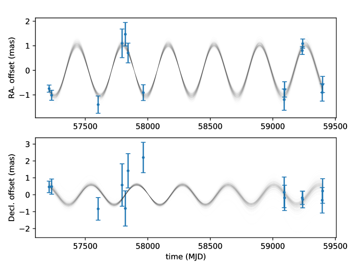
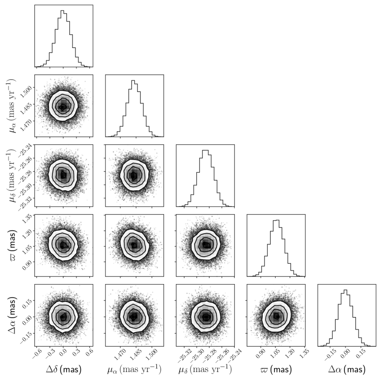
7.5 Testing GR with the orbital decay of PSR J15371155
The observed orbital decay (or the observed time derivative of the orbital period) of J1537 has been estimated to be (Fonseca14) from a global fit of the timing model, which can be attributed to
| (7.1) |
where and stand for the extrinsic orbital decay due to the apparent effect of radial acceleration caused, respectively, by Galactic gravitational potential (Damour91; Nice95) and by transverse motion (Shklovskii70); represents the intrinsic orbital decay as a result of the GW emissions from the inspiraling DNS. The estimation of the two extrinsic orbital-decay terms rely on the distance to J1537, while also depends on the proper motion. On the other hand, the GR-based can be calculated, provided the orbital period , the orbital eccentricity and the masses of the two DNS constituents (Peters63; Weisberg16), all of which have been precisely determined with pulsar timing (Fonseca14). Hence, one can test GR by comparing the observed intrinsic orbital decay with . For J1537, this test is the one (among the tests with PK parameters, see 7.2.1) that showed the largest discrepancy with GR (see Figure 9 of Fonseca14), possibly due to the unreliable DM-based distance used for the test.
Using Equation 22 of Weisberg16, we calculated . Using the proper motion and the distance acquired with Bayesian inference (see 7.2), we updated . The uncertainties for and were derived with error propagation, which were subsequently confirmed by Monte-Carlo simulations. In the error estimation, we did not take into account the small correlation between and (mentioned in 7.4). This is because the correlation between and is still negligible, as the declination component dominates the proper motion (see 7.2).
Following Zhu19, we estimated with different Galactic mass distribution models compiled in GalPot (https://github.com/PaulMcMillan-Astro/GalPot, McMillan17). The results are summarized in 7.3. The errors on can be attributed to two sources: the uncertainty in the measurements (such as distance and proper motion) and the inaccuracy of the Galactic mass distribution model. The former errors, at the level (see 7.3), were derived with Monte-Carlo simulations. We approached the latter errors with the standard deviation of the estimates listed in 7.3. For this calculation of the standard deviation, we do not include the based on the analytical model by Nice95, because 1) the analytical model is oversimplified (see the discussion in Appendix A of Zhu19) and 2) the resultant is inconsistent with other models (see 7.3). Accordingly, we adopted the average of the four remaining Galactic mass distribution models (Dehnen98; Binney11; Piffl14; McMillan17) as the estimate. In this way, we obtained , where the error budget has included the standard deviation (0.14 ) of . As Galpot was not available in 2014, Fonseca14 adopted the based on the Galactic mass distribution model of Nice95 (see 7.3) for the calculation of the timing kinematic distance. Provided our new , the timing kinematic distance of kpc (reported by Fonseca14 and quoted in 7.2) would decrease by 3% to kpc, thus becoming consistent with the new model-independent distance (see 7.2).
| Galactic mass | |||
|---|---|---|---|
| distribution model | () | () | () |
| Nice95 | |||
| Dehnen98 | |||
| Binney11 | |||
| Piffl14 | |||
| McMillan17 | |||
| — | — |
aFor the calculation, we adopted kpc (the distance from the Sun to the Galactic center) provided by Gravity-Collaboration18 and (the circular speed of the local standard of rest). We derived the with the proper motion of Sgr A* (Reid20), the aforementioned (Gravity-Collaboration18) and the velocity of the Sun with respect to the local standard of rest (Schonrich10).
bThere are 4 models discussed in Dehnen98. Here, we used the “model 3”, which falls into the middle of the models 1 to 4, and is generally consistent with the other 3 models.
Collectively, we reached , corresponding to
| (7.2) |
which is the third most precise orbital-decay test of GR in the strong-field regime according to Table 3 of Weisberg16. At the 2% precision level, the new observed intrinsic orbital decay is within of the GR prediction (see 7.3), which relieves the mild tension of the previous test ( at 1.7 agreement, Stairs02).
For visualisation, the mass-mass diagram of J1537 (updated from Figure 9 of Fonseca14) is presented in 7.3, which involves 6 PK parameters. Apart from the 5 PK parameters already mentioned in 7.2, stands for the precession rate of the pulsar. Each PK parameter is a function of the two DNS constituent masses. Therefore, each observed PK parameter (and its uncertainty) offers a constraint on the two masses. If GR is correct, all mass-mass constraints should converge at the “true” masses of the pulsar and its companion. In 7.3, this convergence is visible with the new .
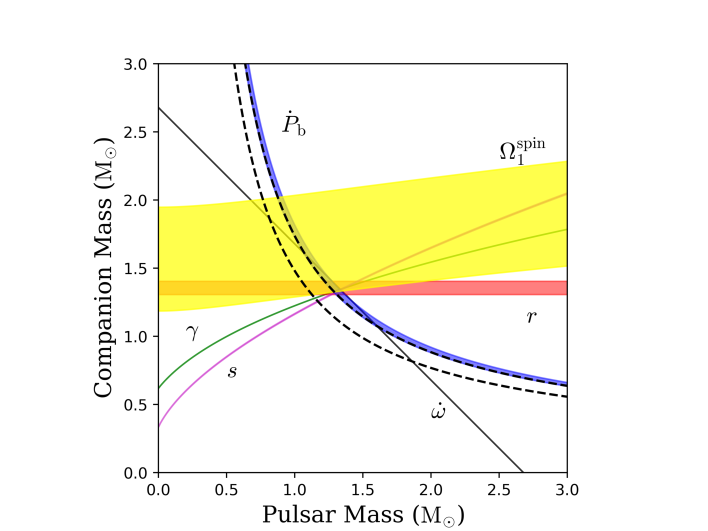
Looking into the future, the bottleneck of the orbital-decay test with J1537 will continue to be its parallax uncertainty, which would decrease with (e.g. Ding21; here, stands for the on-source time instead of the time span) in the long term despite fluctuations of J1537 brightness. This process of precision enhancement would be accelerated with high-sensitivity VLBI observations, as the VLBA observations of J1537 are generally sensitivity-limited, especially when J1537 is down-scintillated.
Acknowledgements
We are grateful to the anonymous referee for the swift and valuable comments, and appreciate the helpful discussions with Leonid Petrov, David Kaplan and Joseph Lazio. B.S. and A.L. thank Mitch Mickaliger for help with timing data acquisition and preparation. H.D. is supported by the ACAMAR (Australia-ChinA ConsortiuM for Astrophysical Research) scholarship, which is partly funded by the China Scholarship Council (CSC). A.T.D is the recipient of an ARC Future Fellowship (FT150100415). Pulsar research at UBC is supported by an NSERC Discovery Grant and by the Canadian Institute of Advanced Research. Pulsar research at JBCA is supported by a Consolidated Grant from STFC. Parts of this research were conducted by the Australian Research Council Centre of Excellence for Gravitational Wave Discovery (OzGrav), through project number CE170100004. This work is based on observations with the Very Long Baseline Array (VLBA), which is operated by the National Radio Astronomy Observatory (NRAO). The NRAO is a facility of the National Science Foundation operated under cooperative agreement by Associated Universities, Inc. Data reduction and analysis was performed on OzSTAR, the Swinburne-based supercomputer. This work made use of the Swinburne University of Technology software correlator, developed as part of the Australian Major National Research Facilities Programme and operated under license.
Chapter 8 VLBI Astrometry of 18 Millisecond Pulsars
This chapter is converted from Ding23 entitled “The catalogue: VLBA astrometry of 18 millisecond pulsars”, which includes the re-analysis of three previously published pulsars (see 6, 7 and Vigeland18). The chapter presents the results for the entire program, although additional observations (now underway) are necessary to achieve the sufficient absolute astrometric precision required for the study of solar system ephemerides (see 1.5.4).
This is the culmination of the thesis, serving a wide range of scientific motivations (see 1.3, 1.4, 1.5, 1.6). Methodologically, the chapter uses all the advanced phase referencing techniques mentioned in 2.2, presents the addition of the systematics-correcting parameter (see 8.5) to the Bayesian astrometric inference package sterne, and applies multi-source astrometric inference for PSR J19392134 (see 8.5.1) with sterne. For the sake of brevity, most figures and tables are submitted as supplementary materials, and meanwhile also made available online. A few minor corrections to this chapter, including the addition of 8.4 and 8.6, are made in response to the comments by the thesis examiners.
8.1 Abstract
With unparalleled rotational stability, millisecond pulsars (MSPs) serve as ideal laboratories for numerous astrophysical studies, many of which require precise knowledge of the distance and/or velocity of the MSP. Here, we present the astrometric results for 18 MSPs of the “” project focusing exclusively on astrometry of MSPs, which includes the re-analysis of 3 previously published MSPs. On top of a standardized data reduction protocol, more complex strategies (i.e., normal and inverse-referenced 1D interpolation) were employed where possible to further improve astrometric precision. We derived astrometric parameters using sterne, a new Bayesian astrometry inference package that allows the incorporation of prior information based on pulsar timing where applicable. We measured significant () parallax-based distances for 15 MSPs, including kpc for PSR J15184904 — the most significant model-independent distance ever measured for a double neutron star system. For each MSP with a well-constrained distance, we estimated its transverse space velocity and radial acceleration. Among the estimated radial accelerations, the updated ones of PSR J10125307 and PSR J17380333 impose new constraints on dipole gravitational radiation and the time derivative of Newton’s gravitational constant. Additionally, significant angular broadening was detected for PSR J16431224, which offers an independent check of the postulated association between the HII region Sh 2-27 and the main scattering screen of PSR J16431224. Last but not least, the upper limit of the death line of -ray-emitting pulsars is refined with the new radial acceleration of the hitherto least energetic -ray pulsar PSR J17302304.
8.2 Introduction
8.2.1 Millisecond pulsars: a key for probing theories of gravity and detecting the gravitational-wave background
Pulsars are an observational manifestation of neutron stars (NSs) that emit non-thermal electromagnetic radiation while spinning (Hewish69; Gold68; Pacini68). Over 3000 radio pulsars have been discovered to date throughout the Galaxy and the nearest members of the Local Group (Manchester05). Due to the large moment of inertia of pulsars, the pulses we receive on Earth from a pulsar exhibit highly stable periodicity. By measuring a train of pulse time-of-arrivals (ToAs) of a pulsar and comparing it against the model prediction, a long list of model parameters can be inferred (e.g. Detweiler79; Helfand80). This procedure to determine ToA-changing parameters is known as pulsar timing, hereafter referred to as timing.
In the pulsar family, recycled pulsars (commonly refereed to as millisecond pulsars, or MSPs), have the shortest rotational periods. They are believed to have been spun-up through the accretion from their donor stars during a previous evolutionary phase as a low-mass X-ray binary (LMXB) (Alpar82). As the duration of the recycling phase (and hence the degree to which the pulsar is spun-up) can vary depending on the nature of the binary, there is no clear cut spin period threshold that separates MSPs from canonical pulsars. In this paper, we define MSPs as pulsars with spin periods of ms and magnetic fields G. This range encompasses most partially recycled pulsars with NS companions, such as PSR J15371155 (aka. PSR B153412) and PSR J15184904. Compared to non-recycled pulsars, ToAs from MSPs can be measured to higher precision due to both the narrower pulse profiles and larger number of pulses. Additionally, MSPs exhibit more stable rotation (e.g. Hobbs10); both factors promise a lower level of random timing noise. Consequently, MSPs outperform non-recycled pulsars in the achievable precision for probing theories underlying ToA-changing astrophysical effects. In particular, MSPs provide the hitherto most precise tests for gravitational theories (e.g. Kramer21a; Zhu19; Freire12). Einstein’s theory of general relativity (GR) is the simplest form among a group of possible candidate post-Newtonian gravitational theories. The discovery of highly relativistic double neutron star (DNS) systems (e.g. Hulse75; Wolszczan91; Burgay03; Lazarus16; Stovall18; Cameron18) and their continued timing have resulted in many high-precision tests of GR and other gravity theories (Fonseca14; Weisberg16; Ferdman20, and especially Kramer21a). The precise timing, optical spectroscopy and VLBI observations of pulsar-white-dwarf (WD) systems have, in addition, achieved tight constraints on several classes of alternative theories of gravity (Deller08; Lazaridis09; Freire12; Antoniadis13; Ding20; Guo21; Zhao22).
Gravitational Waves (GWs) are changes in the curvature of spacetime (generated by accelerating masses), which propagate at the speed of light. Individual GW events in the Hz—kHz range have been detected directly with GW observatories (e.g. Abbott16; see the third Gravitational-Wave Transient Catalog111https://www.ligo.org/science/Publication-O3aFinalCatalog/), and indirectly using the orbital decay of pulsar binaries (e.g. Taylor82; Weisberg16; Kramer21a; Ding21a). Collectively, a gravitational wave background (GWB), formed with primordial GWs and GWs generated by later astrophysical events (Carr80), is widely predicted, but has not yet been confirmed by any observational means. In the range of Hz, supermassive blackhole binaries are postulated to be the primary sources of the GWB (Sesana08). In this nano-hertz regime, the most stringent constraints on the GWB are provided by pulsar timing (Detweiler79).
To enhance the sensitivity for the GWB hunt with pulsar timing, and to distinguish GWB-induced ToA signature from other sources of common timing “noise” (e.g., Solar-system planetary ephemeris error, clock error and interstellar medium, Tiburzi16), a pulsar timing array (PTA), composed of MSPs scattered across the sky (see Roebber19 for spatial distribution requirement), is necessary (Foster90). After 2 decades of efforts, no GWB has yet been detected by a PTA, though common steep-spectrum timing noise (in which GWB signature should reside) has already been confirmed by several major PTA consortia (Arzoumanian20; Goncharov21; Chen21; Antoniadis22).
8.2.2 Very long baseline astrometry of millisecond pulsars
In timing analysis, astrometric information for an MSP (reference position, proper motion, and annual geometric parallax) can form part of the global ensemble of parameters determined from ToAs. However, the astrometric signatures can be small compared to the ToA precision and/or covariant with other parameters in the model, especially for new MSPs that are timed for less than a couple of years (Madison13). Continuing to add newly discovered MSPs into PTAs is considered the best pathway to rapid PTA sensitivity improvement (Siemens13), and is particularly important for PTAs based around newly commissioned high-sensitivity radio telescopes (e.g. Bailes20). Therefore, applying priors to the astrometric parameters can be highly beneficial for the timing of individual MSPs (especially the new ones) and for enhancing PTA sensitivities (Madison13).
Typically, the best approach to independently determine precise astrometric parameters for MSPs is the use of very long baseline interferometry (VLBI) observations, which can achieve sub-mas positional precision (relative to a reference source position) for MSPs in a single observation. By measuring the sky position of a Galactic MSP a number of times and modeling the position evolution, VLBI astrometry can obtain astrometric parameters for the MSP. Compared to pulsar timing, it normally takes much shorter time span to reach a given astrometric precision (e.g. Brisken02; Chatterjee09; Deller19).
One of the limiting factors on searching for the GWB with PTAs is the uncertainties on the Solar-system planetary ephemerides (SSEs) (Vallisneri20), which are utilized to convert geocentric ToAs to ones measured in the (Solar-system) barycentric frame (i.e., the reference frame with respect to the barycentre of the Solar system). In pulsar timing analysis, adopting different SSEs (made by two main producers for various purposes) may lead to discrepant timing parameters (e.g. Wang17). On the other hand, VLBI astrometry measures offsets with respect to a source whose position is measured in a quasi-inertial (reference) frame defined using remote quasars (e.g. Charlot20). Although VLBI astrometry also relies on SSEs to derive annual parallax, it is robust against SSE uncertainties. In other words, for VLBI astrometry, using different SSEs in parameter inference would not lead to a noticeable difference (in the inferred parameters). Therefore, VLBI astrometry of MSPs can serve as an objective standard to be used to discriminate between various SSEs. Specifically, if an SSE is inaccurate, the barycentric frame based on the SSE would display rotation with respect to the quasar-based frame. This frame rotation can be potentially detectable by comparing VLBI positions of multiple MSPs against their timing positions (as measured using a common SSE) (Chatterjee09; Wang17). By eliminating inaccurate SSEs, VLBI astrometry of MSPs can suppress the SSE uncertainties, and hence enhance the PTA sensitivities.
Besides the GWB-related motivations, interferometer-based astrometric parameters (especially distances to MSPs) have been adopted to sharpen the tests of gravitational theories for individual MSPs (e.g. Deller09; Deller18; Guo21; Ding21a). Such tests are normally made by comparing the model-predicted and observed post-Keplerian (PK) parameters that quantify excessive gravitational effects beyond a Newtonian description of the orbital motion. Among the PK parameters is the orbital decay (or the time derivative of orbital period). The intrinsic cause of in double neutron star systems is dominated by the emission of gravitational waves, which can be predicted using the binary constituent masses and orbital parameters (e.g. Lazaridis09; Weisberg16). To test this model prediction, however, requires any extrinsic orbital decay due to relative acceleration between the pulsar and the observer to be removed from the observed . Such extrinsic terms depend crucially on the proper motion and the distance of the pulsar, however these (especially the distance) can be difficult to estimate from pulsar timing. Precise VLBI determination of proper motions and distances can yield precise estimates of these extrinsic terms and therefore play an important role in orbital-decay tests of gravitational theories.
Last but not least, pulsar astrometry is crucial for understanding the Galactic free-electron distribution, or the Galactic free-electron number density as a function of position. An model is normally established by using pulsars with well determined distances as benchmarks. As the pulsations from a pulsar allow precise measurement of its dispersion measure (DM), the average between the pulsar and the Earth can be estimated given the pulsar distance. Accordingly, a large group of such benchmark pulsars across the sky would enable the establishment of an model. In a relevant research field, extragalactic fast radio bursts (FRBs) have been used to probe intergalactic medium distribution on a cosmological scale (e.g. Macquart20; Mannings21), which, however, demands the removal of the DMs of both the Galaxy and the FRB host galaxy. The Galactic DM cannot be determined without a reliable model, which, again, calls for precise astrometry of pulsars across the Galaxy.
8.2.3 The project
Using the Very Long Baseline Array (VLBA), the project tripled the sample of pulsars with precisely measured astrometric parameters (Deller19), but included just three MSPs. The successor project, , is a similarly designed VLBA astrometric program targeting exclusively MSPs. Compared to canonical pulsars, MSPs are generally fainter. To identify MSPs feasible for VLBA astrometry, a pilot program was conducted, which found 31 suitable MSPs. Given observational time constraints, we selected 18 MSPs with the foremost scientific importance as the targets of the project, focusing primarily on sources observed by pulsar timing arrays. The 18 MSPs are listed in 8.1 along with their spin periods and orbital periods (if available) obtained with the ATNF Pulsar Catalogue222https://www.atnf.csiro.au/research/pulsar/psrcat/ (Manchester05). The results for 3 sources (PSR J10125307, PSR J15371155, PSR J16402224) involved in the project have been published (Vigeland18; Ding20; Ding21a). In this paper, we present the astrometric results of the remaining 15 MSPs studied in the project. We also re-derived the results for the 3 published MSPs, in order to ensure consistent and systematic astrometric studies.
| PSR | Gating | Project Codes | Primary phase calibrator | Secondary phase calibrator | IBC | |||||
| (ms) | (d) | gain | (deg) | code | (arcmin) | (mJy) | ||||
| J00300451 | 4.87 | — | 1.75 | BD179B, BD192B | ICRF J002945.8055440 | 0.97 | FIRST J003054.6045908 | 00027 | 10.1 | 20.6 |
| J06102100 | 3.86 | 0.29 | 1.85 | BD179C, BD192C | — | — | NVSS J061002211538 | 00238 | 15.4 | 112.8 |
| J06211002 | 28.85 | 8.3 | 2.15 | BD179D, BD192D | ICRF J061909.9073641 | 2.84 | NVSS J062153102206 | 00303 | 18.1 | |
| J10125307 ∗∗ | 5.26 | 0.60 | 1.43 | BD179E, BD192E | ICRF J095837.8503957 | 3.38 | NVSS J101307531233 | 00462 | 7.51 | 20.8 |
| J10240719 | 5.16 | — | 1.69 | BD179E, BD192E | ICRF J102838.7084438 | 1.59 | FIRST J102526.3072216 | 00529 | 12.2 | 11.7 |
| J15184904 | 40.93 | 8.6 | 2.27 | BD179F, BD192F | ICRF J150644.1493355 | 1.78 | NVSS J151733491626 | 00691 | 35.6 | |
| J15371155 ∗∗ | 37.90 | 0.42 | 1.62 | BD179F, BD192F, BD229 | ICRF J154049.4144745 | 3.18 | FIRST J153746.2114215 | 00840 | 16.3 | 19.2 |
| J16402224 ∗∗ | 3.16 | 175 | 1.90 | BD179G, BD192F | ICRF J164125.2225704 | 0.79 | NVSS J164018221203 | 00920 | 12.1 | 98.0 |
| J16431224 | 4.62 | 147 | 1.56 | BD179G, BD192G | ICRF J163845.2141550 | 2.49 | NVSS J164515122013 | 01120 | 24.3 | 6.0 |
| J17212457 | 3.50 | — | 1.78 | BD179H, BD192H | ICRF J172658.9225801 | 2.47 | NVSS J172129250538 | 01188 | 10.1 | 7.4 |
| J17302304 | 8.12 | — | 1.86 | BD179H, BD192H | ICRF J172658.9225801 | 0.76 | NVSS J172932232722 | 01220 | 25.5 | 37.9 |
| J17380333 | 5.85 | 0.35 | 1.98 | BD179I, BD192I | ICRF J174037.1031147 | 0.66 | NVSS J173823033305 | 01313 | 7.5 | 6.5 |
| J18242452A | 3.05 | — | 1.53 | BD179O, BD192O | ICRF J182057.8252812 | 0.61 | NVSS J182301250438 | 01433 | 3.3 | |
| J18531303 | 4.09 | 116 | 1.64 | BD179K, BD192K | ICRF J185250.5+142639 | 1.51 | NVSS J185456130110 | 01535 | 14.6 | 5.9 |
| J19101256 | 4.98 | 58.5 | 2.65 | BD179L, BD192L | ICRF J191158.2161146 | 3.16 | NVSS J190957130434 | 01769 | 8.7 | 4.9 |
| J19111114 | 3.63 | 2.7 | 1.67 | BD179M, BD192M | ICRF J190528.5115332 | 1.76 | NVSS J191233113327 | 01816 | 21.9 | 23.4 |
| J19180642 | 7.65 | 10.9 | 2.12 | BD179M, BD192M | ICRF J191207.1080421 | 2.14 | NVSS J191731062435 | 01846 | 26.1 | 50.7 |
| J19392134 | 1.56 | — | 1.35 | BD179K, BD192K | ICRF J193510.4203154 | 1.88 | NVSS J194104214913 | 01647 | 10.6 | |
| 1.94 | NVSS J194106215304 | 01648 | 1.8 | |||||||
| The image models for the primary and secondary calibrators listed here are publicly available6. | ||||||||||
| and stand for spin period and orbital period, respectively. | ||||||||||
| ∗ Unresolved flux intensity of the secondary phase calibrator at 1.55 GHz. | ||||||||||
| ∗∗ Published in Ding20; Ding21a; Vigeland18. | ||||||||||
| a Secondary phase calibrators are named IBCXXXXX in the BD179 and BD192 observing files, where “XXXXX” represents a unique 5-digit IBC code. | ||||||||||
| b Angular separation between target and secondary calibrator. | ||||||||||
| c NVSS J061002211538, close to the pulsar on the sky, is bright enough to serve as primary phase calibrator. | ||||||||||
| d As 1D interpolation is applied, the pulsar-to-virtual-calibrator separation is also provided after “” (see 8.4.1). | ||||||||||
| e Here, inverse phase referencing is adopted, where the “secondary phase calibrators” are ultimately the targets (see 8.4.2). | ||||||||||
| f Angular separation between primary and secondary calibrator. | ||||||||||
| g The NVSS J151815491105, a 4.5-mJy-bright source 65 away from the pulsar, is used as the final reference source (see 8.4). | ||||||||||
Along with the release of the catalogue results, this paper covers several scientific and technical perspectives. First, this paper explores novel data reduction strategies such as inverse-referenced 1D phase interpolation (see 8.4.2). Second, a new Bayesian astrometry inference package is presented (see 8.5). Third, with new parallax-based distances and proper motions, we discriminate between the two prevailing models (see 8.7.1), and investigate the kinematics of MSPs in 8.7.2. Fourth, with new parallax-based distances of two MSPs, we re-visit the constraints on alternative theories of gravity (see 8.8). Finally, discussions on individual pulsars are given in 8.9, which includes a refined “death line” upper limit of -ray pulsars (see 8.9.7). The study of SSE-dependent frame rotation, which depends on an accurate estimation of the reference points of our calibrator sources in the quasi-inertial VLBI frame, requires additional multi-frequency observations and will be presented in a follow-up paper.
Throughout this paper, we abide by the following norms unless otherwise stated. 1) The uncertainties are provided at 68% confidence level. 2) Any mention of flux density refers to unresolved flux density in our observing configuration (e.g., a 10-mJy source means mJy). 3) All bootstrap and Bayesian results adopt the 50th, 16th and 84th percentile of the marginalized (and sorted) value chain as, respectively, the estimate and its 1- error lower and upper bound. 4) Where an error of an estimate is required for a specific calculation but an asymmetric error is reported for the estimate, the mean of upper and lower errors is adopted for the calculation. 5) VLBI positional uncertainties will be broken down into the uncertainty of the offset from a chosen calibrator reference point, and the uncertainty in the location of that chosen reference point. This paper focuses on the relative offsets which are relevant for the measurement of proper motion and parallax, and the uncertainty in the location of the reference source is presented separately.
8.3 Observations and Correlation
All MSPs in the catalogue (see Table8.1) were observed at around 1.55 GHz with the VLBA at 2 Gbps data rate from mid-2015 to no later than early 2018. The observing and correlation tactics for the project are identical to those of the project (Deller19). The primary phase calibrators were selected from the Radio Fundamental Catalogue333astrogeo.org/rfc/. The secondary phase calibrators were identified from the FIRST (Faint Images of the Radio Sky at Twenty-cm) catalogue (Becker95) or the NVSS (NRAO VLA sky survey) catalogue (Condon98) (for sky regions not covered by the FIRST survey) using a short multi-field observation. Normally, more than one secondary phase calibrators are identified and observed together with the target. Among them, a main one that is preferably the brightest and the closest to the target is selected to carry out self-calibration; the rest secondary phase calibrators are hereafter referred to as redundant secondary phase calibrators. The primary and the main secondary phase calibrators for the astrometry of the 18 MSPs are summarized in 8.1, alongside the project codes. At correlation time, pulsar gating was applied (Deller11a) to improve the S/N on the target pulsars. The median values of the gating gain, defined as , are provided in 8.1.
8.4 Data Reduction and fiducial systematic errors
We reduced all data with the psrvlbireduce pipeline444available at https://github.com/dingswin/psrvlbireduce written in parseltongue (Kettenis06), a python-based interface for running functions provided by AIPS (Greisen03) and DIFMAP (Shepherd94). The procedure of data reduction is identical to that outlined in Ding20, except for four MSPs — PSR J15184904, PSR J06211002, PSR J18242452A and PSR J19392134. For PSR J15184904, the self-calibration solutions acquired with NVSS J151733491626, a 36-mJy secondary calibrator 138 away from the pulsar, are given to both the pulsar and NVSS J151815491105 — a 4.5-mJy source about a factor of two closer to PSR J15184904 than NVSS J151733491626. The positions relative to NVSS J151815491105 are used to derive the astrometric parameters of PSR J15184904. For the other exceptions, the data reduction procedures as well as fiducial systematics estimation are described in 8.4.1 and 8.4.2.
At the end of the data reduction, a series of positions as well as their random errors (where refers to right ascension or declination at different epochs) are acquired for each pulsar. For each observation, on top of the random errors due to image noise, ionospheric fluctuations would introduce systematic errors that distort and translate the source, the magnitude of which generally increases with the angular separation between a target and its (secondary) phase calibrator (e.g. Chatterjee04; Kirsten15; Deller19). We estimate fiducial values for these systematic errors of pulsar positions using the empirical relation (i.e., Equation 1 of Deller19) derived from the whole sample. While this empirical relation has proven a reasonable approximation to the actual systematic errors for a large sample of sources, for an individual observational setup may overstate or underestimate the true systematic error (see 8.5). We can account for our uncertainty in this empirical estimator by re-formulating the total positional uncertainty as
| (8.1) |
where is a positive correction factor on the fiducial systematic errors. In this work, we assume stays the same for each pulsar throughout its astrometric campaign. The inference of is described in 8.5. We reiterate that the target image frames have been determined by the positions assumed for our reference sources (or virtual calibrators, see 8.4.1), and that any change in the assumed reference source position would transfer directly into a change in the recovered position for the target pulsar. Accordingly, the uncertainty in the reference source position must be accounted for in the pulsar’s reference position error budget, after fitting the pulsar’s astrometric parameters.
All pulsar positions and their error budgets are provided in the online555https://github.com/dingswin/publication_related_materials “pmpar.in.preliminary” and “pmpar.in” files. The only difference between “pmpar.in.preliminary” and “pmpar.in” (for each pulsar) files are the position uncertainties: “pmpar.in.preliminary” and “pmpar.in” offer, respectively, position uncertainties and . As an example, the pulsar positions for PSR J17380333 are presented in 8.2, where the values on the left and right side of the “ — ” sign stand for, respectively, and . Additionally, to facilitate reproducibility, the image models for all primary and secondary phase calibrators listed in 8.1 are released666https://github.com/dingswin/calibrator_models_for_astrometry along with this paper.
| obs. date | (RA.) | (Decl.) |
|---|---|---|
| (yr) | ||
| 2015.6166 | ||
| 2015.8106 | ||
| 2016.6939 | ||
| 2017.1304 | ||
| 2017.2068 | ||
| 2017.2860 | ||
| 2017.2997 | ||
| 2017.7232 | ||
| 2017.7669 | ||
| This table is compiled for PSR J17380333. | ||
| The values on the left and the right side of “ — ” are, respectively, | ||
| statistical errors given in J1738+0333.pmpar.in.preliminary5, and | ||
| systematics-included errors provided in J1738+0333.pmpar.in5. | ||
8.4.1 1D interpolation on PSR J06211002 and PSR J18242452A
One can substantially reduce propagation-related systematic errors using 1D interpolation with two phase calibrators quasi-colinear with a target (e.g. Fomalont03; Ding20c). After 1D interpolation is applied, the target should in effect be referenced to a “virtual calibrator” much closer (on the sky) than either of the two physical phase calibrators, assuming the phase screen can be approximated by a linear gradient with sky position (Ding20c).
According to 8.1, 7 secondary phase calibrators (or the final reference sources) are more than 20’ away from their targets, which would generally lead to relatively large systematic errors (e.g. Chatterjee04; Kirsten15; Deller19). Fortunately, there are 3 MSPs — PSR J06211002, PSR J18242452A and PSR J19392134, for which the pulsar and its primary and secondary phase calibrators are near-colinear (see online5 calibrator plans as well as 8.1). Hence, by applying 1D interpolation, each of the 3 “1D-interpolation-capable” MSPs can be referenced to a virtual calibrator much closer than the physical secondary phase calibrator (see 8.1).
We implemented 1D interpolation on PSR J06211002 and PSR J18242452A in the same way as the astrometry of the radio magnetar XTE J1810197 carried out at 5.7 GHz (Ding20c). Nonetheless, due to our different observing frequency (i.e., 1.55 GHz), we estimated differently. The post-1D-interpolation systematic errors should consist of 1) first-order residual systematic errors related to the target-to-virtual-calibrator offset and 2) higher-order terms. Assuming negligible higher-order terms, we approached post-1D-interpolation with Equation 1 of Deller19, using as the calibrator-to-target separation. The assumption of negligible higher-order terms will be tested later and discussed in 8.5.1.
8.4.2 Inverse-referenced 1D interpolation on PSR J19392134
For PSR J19392134, normal 1D interpolation (Fomalont03; Ding20c) is still not the optimal calibration strategy. The 10-mJy (at 1.55 GHz) PSR J19392134 is the brightest MSP in the northern hemisphere and only second to PSR J04374715 on the whole sky. After pulsar gating, PSR J19392134 is actually brighter than the brightest secondary reference source NVSS J194104214913 (hereafter referred to as J194104). PSR J19392134 is unresolved on VLBI scales, and does not show long-term radio feature variations (frequently seen in quasars), which makes it an ideal secondary phase calibrator. Both factors encouraged us to implement the inverse-referenced 1D interpolation (or simply inverse 1D interpolation) on PSR J19392134, where PSR J19392134 is the de-facto secondary phase calibrator and the two “secondary phase calibrators” serve as the targets. To avoid confusion, we refer to the two “secondary phase calibrators” for PSR J19392134 (see 8.1) as secondary reference sources or simply reference sources.
Though inverse phase referencing (without interpolation) has been an observing/calibration strategy broadly used in VLBI astrometry (e.g. Imai12; Yang16; Li18; Deller19), inverse interpolation is new, with the 2D approach of Hyland22 at 8.3 GHz being a recent and independent development. We implemented inverse 1D interpolation at 1.55 GHz on PSR J19392134 in three steps (in addition to the standard procedure) detailed as follows.
Tying PSR J19392134 to the primary-calibrator reference frame
Inverse 1D interpolation relies on the residual phase solutions of self-calibration on PSR J19392134 (where , and refers to, respectively, sky position, time and the -th station in a VLBI array), which, however, change with — the displacement from the “true” pulsar position to its model position. When is much smaller than the synthesized beam size , the changes in would be equal across all epochs, hence not biasing the resultant parallax and proper motion. However, if , then the phase wraps of would likely become hard to uncover. The main contributor of considerable is an inaccurate pulsar position. The proper motion of the pulsar would also increase with time, if it is poorly constrained (or neglected). For PSR J19392134, the effect of proper motion across our observing duration is small compared to mas.
In order to minimize , we shifted the pulsar model position, on an epoch-to-epoch basis, by (which ideally should approximate ), to the position measured in the J1935 reference frame (see Section 4.1 of Ding20c for explanation of “reference frame”). This J1935-frame position was derived with the method for determining pulsar absolute position (Ding20) (where J194104 was used temporarily as the secondary phase calibrator) except that there is no need to quantify the position uncertainty. We typically found mas, which is well above mas. After the map centre shift, PSR J19392134 becomes tied to the J1935 frame.
1D interpolation on the tied PSR J19392134
The second step of inverse 1D interpolation is simply the normal 1D interpolation on PSR J19392134 that has been tied to the J1935 frame as described above (in 8.4.2). When there is only one secondary reference source, optimal 1D interpolation should see the virtual calibrator moved along the interpolation line (that passes through both J1935 and PSR J19392134) to the closest position to the secondary reference source (e.g. Ding20c). However, there are two reference sources for PSR J19392134 (see 8.1), and the virtual calibrator point can be set at a point that will enable both of them to be used.
After calibration, a separate position series can be produced for each reference source. While we used each reference-source position series to infer astrometric parameters separately, we can also directly infer astrometric parameters with the combined knowledge of the two position series (which can be realized with 777https://github.com/dingswin/sterne). If the errors in the two position series are (largely) uncorrelated, this can provide superior astrometric precision. Since position residuals should be spatially correlated, we would ideally set the virtual calibrator at a location such that the included angle between the two reference sources is . While achieving this ideal is not possible, we chose a virtual calibrator location that forms the largest possible included angle (657) with the two reference sources to minimise spatially correlated errors (see 8.1). This virtual calibrator is 1.2836 times further away from J1935 than PSR J19392134. Accordingly, the solutions (obtained from the self-calibration on the tied PSR J19392134) were multiplied by 1.2836, and applied to the two reference sources.
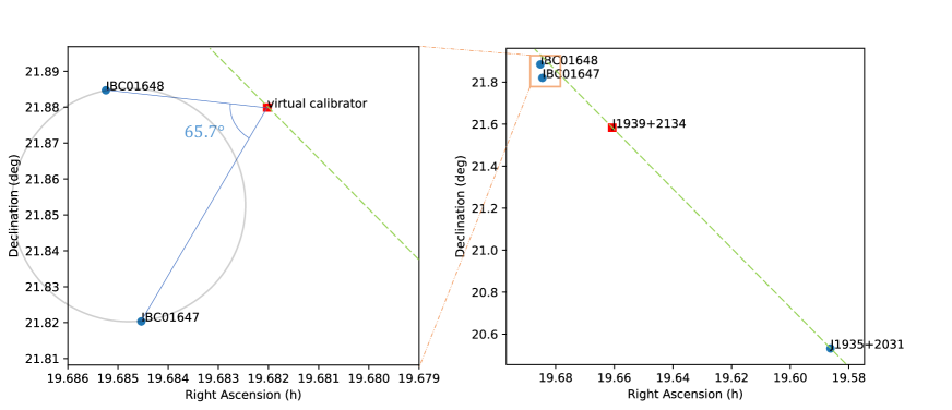
De-shifting reference source positions
After data reduction involving the two steps outlined in 8.4.2 and 8.4.2, one position series was acquired for each reference source. At this point, however, the two position series are not yet ready for astrometric inference, mainly because both proper motion and parallax signatures have been removed in the first step (see 8.4.2) when PSR J19392134 was shifted to its J1935-frame position. Therefore, the third step of inverse 1D interpolation is to cancel out the PSR J19392134 shift (made in the first step) by moving reference source positions by , where the multiplication can be understood by considering Figure 1 of Ding20c. This de-shifting operation was carried out separately outside the data reduction pipeline4. After the operation, we estimated of the reference sources (where refers to an individual reference source) following the method described in 8.4.1. The final position series of the reference sources are available online5. The astrometric parameter inference based on these position series is outlined in 8.5.
8.5 Astrometric inference methods and quasi-VLBI-only astrometric results
After gathering the position series5 with basic uncertainty estimation (see 8.4), we proceed to infer the astrometric parameters. The inference is made by three different methods: a) direct fitting of the position series with pmpar888https://github.com/walterfb/pmpar, b) bootstrapping (see Ding20) and c) Bayesian analysis using sterne7 (see Ding21a). The two former methods directly adopt as the position errors. In Bayesian analysis, however, we followed Lentati14 and inferred along with other model parameters using the likelihood terms
| (8.2) |
where obeys 8.1; refers to the model offsets from the measured positions. To prevent possible confusion, we note here that is defined differently from the “EFAC” specified by Equation 10 of Lentati14. As is discussed in 8.5.2, Bayesian inference outperforms the other two methods, and is hence consistently used to present final results in this work. In all cases, the uncertainty in the reference source position should be added in quadrature to the uncertainty in the pulsar’s reference position acquired with any method (of the three), in order to obtain a final estimate of the absolute positional uncertainty of the pulsar.
To serve different scientific purposes, we present two sets of astrometric results in two sections (i.e., 8.5 and 8.6), which differ in whether timing proper motions and parallaxes are used as prior information in the inference.
Priors of canonical model parameters used in Bayesian analysis
To facilitate reproduction of our Bayesian results, the priors (of Bayesian inference) we use for canonical model parameter are detailed as follows. Priors for the two orbital parameters can be found in 8.5.3. We universally adopt the prior uniform distribution (0, 15) (i.e., uniformly distributed between 0 and 15) for . This prior distribution can be refined for future work with an ensemble of results across many pulsars. With regard to the canonical astrometric parameters (7 parameters for PSR J19392134 and 5 for the other pulsars), we adopt for each , where refers to one of , , , and . Here, stands for the direct-fitting estimate of ; represents the direct-fitting error corrected by the reduced chi-square (see 8.3) with . The calculation of prior range of is made with the function 7.
8.5.1 Astrometric inference disregarding orbital motion
Single-reference-source astrometric inferences
All MSPs (in this work) excepting PSR J19392134 have only one reference source. For each of these single-reference-source MSPs, we fit for the five canonical astrometric parameters, i.e., reference position ( and ), proper motion ( and ) and parallax (). In the Bayesian analysis alone, is also inferred alongside the astrometric parameters. At this stage, we neglect any orbital reflex motion for binary pulsars – the effects of orbital reflex motion are addressed in 8.5.3. The proper motions and parallaxes derived with single-reference-source astrometry and disregarding orbital motion are summarized in 8.3. The reference positions are presented in 8.5.4.
| PSR | |||||||||||||
| () | () | (mas) | () | () | (mas) | () | () | (mas) | (d) | ||||
| Non-1D-interpolated results | |||||||||||||
| J00300451 | -6.13(4) | 0.33(9) | 3.02(4) | 1.4 | -6.1(1) | -6.13(7) | 3.02(7) | — | — | ||||
| J06102100 | 9.11(8) | 15.9(2) | 0.74(7) | 1.0 | 15.9(2) | 9.1(1) | 0.73(10) | 0.29 | |||||
| J06211002 | 3.51(9) | -1.32(16) | 0.88(7) | 3.7 | -1.3(2) | 3.4(2) | -1.3(5) | 0.85(21) | 0.4 | 8.3 | |||
| J10125307 | 2.68(3) | -25.38(6) | 1.17(2) | 1.9 | -25.39(12) | 2.67(5) | 0.1 | 0.60 | |||||
| J10240719 | -35.32(4) | -48.2(1) | 0.94(3) | 1.1 | -48.2(1) | -35.32(7) | -48.1(2) | 0.94(6) | — | — | |||
| J15184904 | -0.69(2) | -8.54(4) | 1.24(2) | 1.2 | -0.69(3) | 1.25(3) | -0.69(3) | -8.52(7) | 1.24(3) | 4.9 | 8.6 | ||
| J15371155 | 1.51(2) | -25.31(5) | 1.06(7) | 0.81 | 1.51(2) | 1.51(3) | 0.24 | 0.42 | |||||
| J16402224 | 2.199(56) | -11.29(9) | 0.676(46) | 1.1 | - | 2.20(9) | 0.68(7) | 3.1 | 175 | ||||
| J16431224 | 6.2(2) | 3.3(5) | 1.3(1) | 0.8 | 3.3(4) | 6.2(2) | 3.3(6) | 1.33(18) | 1.1 | 147 | |||
| J17212457 | 2.5(1) | -1.9(3) | 0.02(7) | 4.4 | 2.5(6) | 2.5(3) | -1.9(9) | 0.0(2) | — | — | |||
| J17302304 | 20.3(1) | -4.79(26) | 1.56(9) | 1.7 | 20.3(2) | -4.8(5) | — | — | |||||
| J17380333 | 6.97(4) | 5.18(7) | 0.51(3) | 1.8 | 5.2(1) | 6.98(8) | 5.18(16) | 0.50(6) | 0.02 | 0.35 | |||
| J18242452A | -0.03(49) | -6.6(1.2) | -0.25(37) | 0.8 | -0.1(6) | -6.6(1.5) | -0.22(48) | — | — | ||||
| J18531303 | -1.37(9) | -2.8(2) | 0.49(6) | 1.0 | -2.8(2) | -1.36(10) | -2.8(2) | 0.50(6) | 1.4 | 116 | |||
| J19101256 | 0.49(8) | -6.85(15) | 0.26(7) | 0.15 | -6.85(6) | 0.50(4) | -6.85(9) | 0.25(3) | 0.87 | 58.5 | |||
| J19111114 | -13.8(1) | -10.3(2) | 0.38(9) | 0.9 | 0.36(8) | -13.8(2) | -10.3(4) | 2.7 | |||||
| J19180642 | -7.12(8) | -5.7(2) | 0.60(7) | 1.1 | -7.1(1) | -7.1(1) | -5.7(3) | 0.60(12) | 0.27 | 10.9 | |||
| J19392134 | 0.07(14) | -0.24(24) | 0.35(10) | 0.2 | 0.08(10) | 0.34(7) | — | — | |||||
| Single-reference-source 1D-interpolated results | |||||||||||||
| J06211002 | 3.68(6) | -1.33(9) | 0.94(4) | 6.3 | -1.3(2) | 3.5(2) | -1.37(35) | 0.86(15) | 0.4 | 8.3 | |||
| J18242452A | 0.3(3) | -3.7(6) | 0.1(3) | 1.5 | 0.3(6) | 0.1(5) | — | — | |||||
| J19392134 | 0.08(4) | -0.45(6) | 0.38(3) | 1.3 | 0.08(7) | -0.44(11) | — | — | |||||
| J19392134 | 0.3(3) | -0.3(2) | 0.36(19) | 1.3 | -0.3(4) | 0.3(4) | -0.3(4) | — | — | ||||
| Multi-reference-source 1D-interpolated results | |||||||||||||
| J19392134 | — | —- | — | — | — | — | — | 0.08(7) | -0.43(11) | — | — | ||
| “DF”, “Bo” and “Ba” stands for, respectively, direct fitting, bootstrap and Bayesian inference. is the reduced chi-square of direct fitting using pmpar8. | |||||||||||||
| The middle and top block presents, respectively, 1D-interpolated (see 8.4.1 and 8.4.2) and non-1D-interpolated results. | |||||||||||||
| The bottom entry for PSR J19392134 shows the result of multi-reference-source astrometry inference (see 8.5.1). | |||||||||||||
| represents orbital period (see Table 4 for their references). is defined in 8.3. | |||||||||||||
| ∗ Already published in Vigeland18; Ding20; Ding21a. | |||||||||||||
| (i) Based on (non-1D-interpolated) J194104 positions inverse-referenced to PSR J19392134. | |||||||||||||
| (ii) Using 1D-interpolated J194104 positions inverse-referenced to PSR J19392134. | |||||||||||||
| (iii) Using 1D-interpolated J194106 positions inverse-referenced to PSR J19392134. | |||||||||||||
| (iv) Based on 1D-interpolated J194104 and J194106 positions inverse-referenced to PSR J19392134 (see 8.4.2). | |||||||||||||
Multi-source astrometry inferences
When multiple sources share proper motion and/or parallax (while each source having its own reference position), a joint multi-source astrometry inference can increase the degrees of freedom of inference (i.e., the number of measurements reduced by the number of parameters to infer), and tighten constraints on the astrometric parameters. Multi-source astrometry inference has been widely used in maser astrometry (where maser spots with different proper motions scatter around a region of high-mass star formation, Reid09a), but has not yet been used for any pulsar, despite the availability of several bright pulsars with multiple in-beam calibrators (e.g., PSR J03325434, PSR J11361551) in the project (Deller19).
PSR J19392134 is the only source (in this work) that has multiple (i.e., two) reference sources, which provides a rare opportunity to test multi-reference-source astrometry. We assumed that the position series of J194104 is uncorrelated with that of NVSS J194106215304 (hereafter J194106), and utilized sterne7 to infer the common parallax and proper motion, alongside two reference positions (one for each reference source). The acquired proper motion and parallax are listed in 8.3. As inverse phase referencing is applied for PSR J19392134, the parallax and proper motion of PSR J19392134 are the inverse of the direct astrometric measurements. For comparison, the proper motion and parallax inferred solely with one reference source are also reported in 8.3. Due to the relative faintness of J194106 (see 8.1), the inclusion of J194106 only marginally improves the astrometric results (e.g., ) over those inferred with J194104 alone.
The constraints on the parallax (as well as the proper motion) are visualized in 8.2. The best-inferred model (derived from the J194104 and J194106 positions) is illustrated with a bright magenta curve, amidst two sets of Bayesian simulations — each set for a reference source. Each simulated curve is a time series of simulated positions, with the best-inferred reference position ( and , where refers to either J194104 or J194106) and proper-motion-related displacements (i.e., and , where is the time delay from the reference epoch) subtracted. As the simulated curve depends on the underlying model parameters, the degree of scatter of simulated curves would increase with larger uncertainties of model parameters. Though sharing simulated parallaxes and proper motions with J194104, the simulated curves for J194106 exhibits broader scatter (than the J194104 ones) owing to more uncertain reference position (see 8.5.4 for and ). The large scatter implies that the J194106 position measurements impose relatively limited constraints on the common model parameter (i.e., parallax and proper motion), which is consistent with the findings from 8.3.
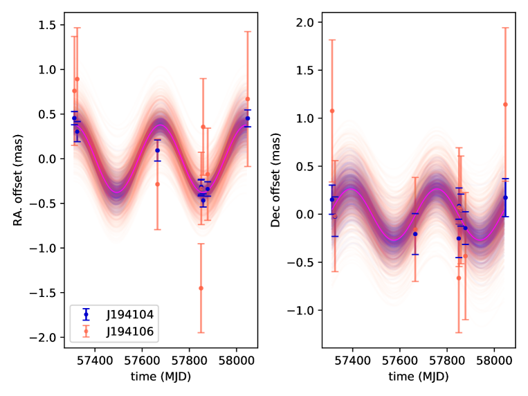
Implications for 1D/2D interpolation
On the three 1D-interpolation-capable MSPs, we compared astrometric inference with both the 1D-interpolated and non-1D-interpolated position series (one at a time). For PSR J19392134, the of the three 1D-interpolated realizations are consistent with each other, but larger than the non-1D-interpolated counterpart. This post-1D-interpolation inflation of also occurs to the other two 1D-interpolation-capable pulsars (see 8.3), which suggests the post-1D-interpolation fiducial systematic errors might be systematically under-estimated. One obvious explanation for this under-estimation is that the higher-order terms of systematic errors are non-negligible (as opposed to the assumption we started with in 8.4.1): they might be actually comparable to the first-order residual systematic errors (that are related to ) at the GHz observing frequencies.
On the other hand, the astrometric results based on the non-1D-interpolated J194104 positions inverse-referenced to PSR J19392134 are less precise than the 1D-interpolated counterpart by % , as is also the case for PSR J06211002 (see 8.3). Moreover, the post-1D-interpolation parallax of PSR J18242452A becomes relatively more accurate than the non-1D-interpolation negative counterpart. All of these demonstrate the utility of 1D/2D interpolation, even in the scenario of in-beam astrometry that is already precise. In the remainder of this paper, we only focus on the 1D-interpolated astrometric results for the three 1D-interpolation-capable MSPs.
8.5.2 Bayesian inference as the major method for
We now compare the three sets of astrometric parameters (in 8.3) obtained with different inference methods, and seek to proceed with only one set in order to simplify the structure of this paper. Among the three inference methods we use in this work, direct least-square fitting is the most time-efficient, but is also the least robust against improperly estimated positional uncertainties. Conversely, the other two methods (i.e., bootstrap and Bayesian methods) do not rely solely on the input positional uncertainties, and can still estimate the model parameters and their uncertainties ( or ; “Bo” or “Ba”) more robustly in the presence of incorrectly estimated positional errors.
Generally speaking, inferred from a pulsar position series are expected to change with the corresponding -corrected direct-fitting error . In order to investigate the relation between and , we divided by for each pulsar entry in the top block of 8.3. The results are displayed in 8.3. For the convenience of illustration, we calculated the dimensionless defined as (where represents the standard deviation of over the group ), which allows all the three sets (i.e., , and ) of dimensionless to be horizontally more evenly plotted in 8.3.
Across the entire sample, we see that scales with in a near-linear fashion. The mean scaling factors across all of the three parameter groups (i.e., , and ) are and (see 8.3). The two mean scaling factors show that parameter uncertainties inferred using either a bootstrap or Bayesian approach will be slightly higher (and on average, consistent between the two approaches) than would be obtained utilising direct-fitting (illustrated with the cyan dashed line in 8.3).
The more optimistic uncertainty predictions of can be understood as resulting from two causes: first, it neglects both the finite width and the skewness of the distribution, and second, to achieve the expected it scales the total uncertainty contribution at each epoch, rather than the systematic uncertainty contribution alone. When (as is typical for pulsar observations) the S/N and hence statistical positional precision can vary substantially between observing epochs, this simplified approach preserves the relative weighting between epochs, whereas increasing the estimated systematic uncertainty contribution acts to equalise the weighting between epochs (by reducing the position precision more for epochs where the pulsar was bright and the statistical precision high, than for epochs where the pulsar was faint and the statistical precision is already low).
While the consistency between and suggests that both approaches can overcome this shortcoming in the direct fitting method, shows a much larger scatter (3.5 times) compared to (see 8.3). To determine which approach best represents the true (and unknown) parameter uncertainties, it is instructive to consider the outliers in the bootstrap distribution results.
First, consider cases where the bootstrap results in a lower uncertainty than . For the reasons noted above, we expect to yield the most optimistic final parameter uncertainty estimates, and yet the bootstrap returns a lower uncertainty than in a number of cases. Second, the cases with the highest values of reach 3 on a number of occasions, which imply an extremely large (or very non-Gaussian) systematic uncertainty contribution, which would lead (in those cases) to a surprisingly low reduced for the best-fitting model. Given the frequency with which these outliers arise, we regard it likely that bootstrap approach mis-estimates parameter uncertainties at least occasionally, likely due to the small number of observations available.
Therefore, we consider the Bayesian method described in this paper as the preferred inference method for the sample, and consistently use the Bayesian results in the following discussions. We note that as continued VLBI observing campaigns add more results, the systematic uncertainty estimation scheme applied to Bayesian inference can be further refined in the future.
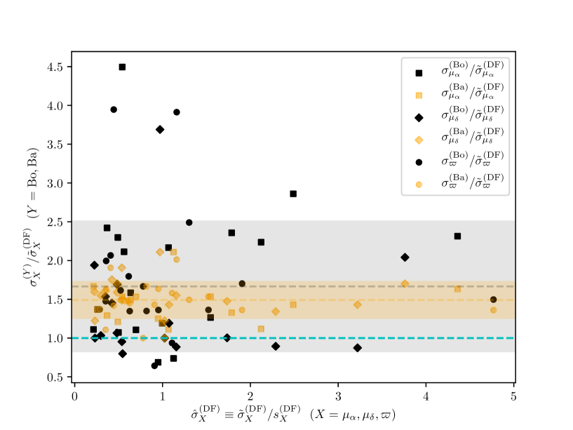
8.5.3 Astrometric inference accounting for orbital motion
For some binary pulsars, VLBI astrometry can also refine parameters related to the binary orbit, on top of the canonical astrometric parameters. The orbital inclination and the orbital ascending node longitude have been previously constrained for a few nearby pulsars, such as PSR J10221001, PSR J21450750 and PSR J22220137 (Deller13; Deller16; Guo21). To assess the feasibility of detecting orbital reflex motion with VLBI, we computed
| (8.3) |
where and stands for, respectively, the distance (to the pulsar) and the orbital semi-major axis projected onto the sightline. On the other hand, reflects the apparent angular size of orbit. Provided the parallax uncertainty , quantifies the detectability of orbital parameters using VLBI astrometry. Hence,
| (8.4) |
Since is usually unknown, the defined in 8.3 serves as a lower limit for , and is used in this work to find out pulsar systems with and potentially measurable with VLBI observations. In general, the orbital reflex motion should be negligible when , easily measurable when , and difficult to constrain (but non-negligible) when . By way of comparison, Guo21 were able to firmly constrain and for PSR J22220137 (), while Deller16 could place weak constraints for PSR J10221001 and PSR J21450750 ( and 1.6, respectively)
Accordingly, in this work, we fit for orbital reflex motion if all the following conditions are met:
-
(i)
is well determined with pulsar timing;
-
(ii)
;
-
(iii)
the orbital period yr, where 2 yr is the nominal time span of an astrometric campaign.
For the calculation of , we simply use the direct-fitting parallax for , and its -corrected uncertainty for (see 8.3). The calculated as well as are summarized in 8.3. Among the 18 pulsars, PSR J15184904, PSR J16402224, PSR J16431224 and PSR J18531303 meet our criteria (see 8.3). Hereafter, the 4 pulsars are referred to as the “8P” pulsars for the sake of brevity, as we would perform 8-parameter (i.e., the 5 canonical astrometric parameters and plus and ) inference on them.
For the 8-parameter inference, prior probability distributions of the canonical parameters and are described in 8.5. Both and are defined in the TEMPO2 (Edwards06) convention. The prior probability distribution of follows (0, 360∘). Sine distribution (0, 180∘) is used for of the four 8P pulsars (i.e., the probability density , ). Where available, tighter constraints are applied to in accordance with 8.4 (also see the descriptions in 8.9).
Moreover, extra prior constraints can be applied to and based on , the time derivative of (e.g. Nice01; Deller16; Reardon21). As ,
| (8.5) |
Here, the term reflects the intrinsic variation of the semi-major axis due to GR effects (Peters64), which is however 8 and 5 orders smaller than for the 8P WD-pulsar systems and the DNS system PSR J15184904, respectively (see Nice01 for an analogy). Accordingly, the apparent is predominantly caused by apparent change as a result of the sightline shift (Kopeikin96). When proper motion contributes predominantly to the sky position shift (as is the case for the 8P pulsars),
| (8.6) |
where refers to the position angle (east of north) of the proper motion (Kopeikin96; Nice01). We incorporated the measurements (with 8.5 and 8.6) on top of other prior constraints, and inferred , , and the canonical five astrometric parameters for the 8P pulsars with sterne7, following similar approaches taken by Deller16; Guo21.
While we ultimately did not significantly constrain or for any pulsars, including their non-negligible reflex motion in the inference is still necessary for correctly inferring the uncertainties of the non-orbital model parameters. The non-orbital inferred parameters are provided in 8.5.4 below, along with all the non-8P pulsars. As we found minimal differences between the constraints obtained on orbital parameters with or without the adoption of priors based on pulsar timing, we defer the presentation of the posterior constraints on orbital inclinations and ascending node longitudes (of the 8P pulsars) to 8.6 in order to avoid repetition.
| PSR | ||||
| () | () | (deg) | ||
| J15184904 | -11(3) | -0.55(15) | — | |
| J16402224 | 12(1) d | 0.22(2) | d | — |
| J16431224 | -49.7(7) c | -1.98(3) | — | — |
| J18531303 | 14(2) d | 0.34(5) | 85(14)∘ b | — |
| Janssen08; inferred from the non-detection of Shapiro delay effects. | ||||
| b based on Shapiro delay measurements (Faisal-Alam20). | ||||
| cReardon21; dPerera19. | ||||
8.5.4 The quasi-VLBI-only astrometric results
To wrap up this section, we summarize in 8.5 the full (including and ) final astrometric results obtained with no exterior prior proper motion or parallax constraints, which we simply refer to as quasi-VLBI-only astrometric results (we add “quasi” because timing constraints on two orbital parameters, i.e., and , have already been used for the 8P pulsars). These quasi-VLBI-only results are mainly meant for independent checks of timing results (which would enable the frame connection mentioned in 8.2.2), or as priors for future timing analyses. For the most precise possible pulsar parallaxes and hence distances, we recommend the use of the “VLBI timing” results presented in 8.6.
| PSR | (J2000) ∗ | (J2000) ∗ | |||||||||
| (MJD) | (mas) | (mas) | () | () | (mas) | ||||||
| J00300451 | 57849 | -6.13(7) | 3.02(7) | 0.39 | 0.08 | ||||||
| J06102100 | 57757 | 9.1(1) | 0.73(10) | 0.51 | 0.05 | ||||||
| J06211002 | 57685 | 3.5(2) | -1.37(35) | 0.86(15) | 0.60 | -0.01 | |||||
| J10125307 | 57700 | 2.67(5) | 0.37 | -0.06 | |||||||
| J10240719 | 57797 | -35.32(7) | -48.1(2) | 0.94(6) | 0.23 | ||||||
| J15184904 b | 57795 | 1.238(36) | -0.19 | -0.68 | |||||||
| J15371155 | 57964 | 1.51(3) | -0.17 | 0.04 | |||||||
| J16402224 b | 57500 | 2.19(9) | 0.68(8) | -0.57 | -0.02 | ||||||
| J16431224 b | 57700 | 6.2(2) | 3.3(6) | -0.43 | 0.04 | ||||||
| J17212457 | 57820 | 2.5(3) | -1.9(9) | 0.0(2) | -0.13 | -0.01 | |||||
| J17302304 | 57821 | 20.3(2) | -4.8(5) | -0.38 | 0.01 | ||||||
| J17380333 | 57829 | 6.98(8) | 5.18(16) | 0.50(6) | -0.53 | ||||||
| J18242452A | 57836 | 0.3(6) | 0.1(5) | -0.65 | |||||||
| J18531303 b | 57846 | -1.4(1) | -2.8(2) | 0.49(7) | -0.37 | 0.26 | |||||
| J19101256 | 57847 | 0.50(4) | -6.85(9) | 0.254(35) | -0.48 | 0.03 | |||||
| J19111114 | 57768 | -13.8(2) | -10.3(4) | -0.39 | -0.02 | ||||||
| J19180642 | 57768 | -7.1(1) | -5.7(3) | 0.60(12) | -0.39 | -0.01 | |||||
| J19392134 a | 57850 | 0.08(7) | -0.43(11) | -0.62 | -0.06 | ||||||
| ∗ and refer to the reference position at reference epoch . The error budgets of the reference positions are provided in the adjacent columns, which include, from left to right, the error of relative | |||||||||||
| reference position with respect to the reference point, the uncertainty of the reference point with regard to the main phase calibrator (estimated with Equation 1 of Deller19), the position uncertainty | |||||||||||
| of the main phase calibrator, and the typical (0.8 mas in each direction, Sokolovsky11) frequency-dependent core shift (e.g. Bartel86; Lobanov98) between 1.55 GHz and GHz. | |||||||||||
| We note that the errors outside “[ ]” are obtained with Bayesian inference, while the errors inside “[ ]” are only indicative. To properly determine the absolute pulsar position and its uncertainty requires | |||||||||||
| the procedure described in Section 3.2 of Ding20. This analysis will be made and presented in an upcoming paper. | |||||||||||
| and stand for correlation coefficients between and the two proper motion components. | |||||||||||
| The special parameter (that has been provided in 8.3 and 8.4) is not reiterated in this table. | |||||||||||
| a Since inverse referencing is applied for PSR J19392134, the two reference sources are the de-facto targets. Accordingly, the proper motion and parallax are the negative values of the direct measurements out | |||||||||||
| of inverse referencing. For the original astrometric model, the reference positions for the two reference sources J194104 and J194106 are, respectively, and | |||||||||||
| , where the uncertainties do not contain those of the reference point (i.e. the inside-the-bracket terms of and ). The reference position of PSR J19392134 | |||||||||||
| presented in the table is estimated using normal phase referencing with respect to J194104. | |||||||||||
| b Results of the 8-parameter Bayesian inference are reported here; the constraints on and are described in 8.6 (see 8.5.3 for explanations). | |||||||||||
The reference positions and we provide in 8.5 are precisely measured, but only with respect to the assumed location of the in-beam calibrator source for each pulsar. In all cases, the uncertainties on the in-beam source locations (also shown in 8.5) dominate the total uncertainty in the pulsar’s reference position. A future work, incorporating additional multi-frequency observations of the in-beam calibrations, will enable significantly more precise pulsar reference positions to be obtained, as is discussed in 8.2.3.
8.6 VLBI+timing astrometric results
In Bayesian inference, the output of a model parameter (where refers to various model parameters) hinges on its prior probability distribution: generally speaking, tighter prior constraints (on ) that are consistent with data (in the sense of Bayesian analysis) would sharpen the output . In cases where a strong correlation between and another model parameter is present, tighter prior constraints consistent with the data would potentially sharpen both the output and the output .
As noted in 8.2.2, VLBI astrometry serves as the prime method to measure parallaxes of Galactic pulsars. A VLBI astrometric campaign (on a Galactic pulsar) normally spans years, as a substantial parallax can likely be achieved in this timespan. On the other hand, most pulsars have been timed routinely for years, which allows their proper motions to be precisely determined, as the precision on proper motion grows with for a regularly observed pulsar. In 8.6, we collect one timing proper motion (denoted as and ) and one timing parallax () for each pulsar. Among the published timing results, we select the timing proper motions measured over the longest timespan, and the having the smallest uncertainties. 8.4 is produced to visualize the difference between the quasi-VLBI-only proper motions and the timing ones. According to 8.5, 8.6 and 8.4, most timing proper motions are more precise than the quasi-VLBI-only counterparts. On the other hand, timing parallaxes are mostly less precise than the quasi-VLBI-only counterparts. Nevertheless, adopting appropriate timing parallaxes as priors can still effectively lower parallax uncertainties.
The precisely measured and provide the opportunity to significantly refine the quasi-VLBI-only proper motions. Furthermore, as shown with the Pearson correlation coefficients (Pearson95) and that we summarized in 8.5, large correlation between parallax and proper motion is not rare for VLBI astrometry. Therefore, using the and measurements as the prior proper motion constraints in Bayesian inference can potentially refine both proper motion and parallax determination.
The astrometric results inferred with timing priors, hereafter referred to as VLBI+timing results, are reported in 8.6. To differentiate from the notation of quasi-VLBI-only astrometric parameter , we denote a VLBI+timing model parameter in the form of . Comparing 8.5 and 8.6, we find almost all VLBI+timing proper motions and parallaxes more precise than the quasi-VLBI-only counterparts; the most significant parallax precision enhancement occurs to PSR J19180642 (by 42%), followed by PSR J19392134 (by 36%) and PSR J15371155 (by 33%). Hence, we use the VLBI+timing results in the remainder of this paper.
In 7 cases (i.e., PSR J06102100, PSR J16431224, PSR J17302304, PSR J17380333, PSR J18531303, PSR J18242452A, PSR J19101256), one of , or is more than 2 discrepant from the quasi-VLBI-only counterpart. Using such timing priors may widen the uncertainties of resultant model parameters, as would be lifted to counter-balance the increased . Without any indication that the discrepant timing values are less reliable, we use them as priors regardless. However, we caution the use of these 7 sets of VLBI+timing results, and would recommend the quasi-VLBI-only results to be considered if our adopted timing priors are proven inaccurate in future.
We also now consider any possible effects that could, despite our best efforts to characterise all sources of position noise, bias the fitted VLBI positions. For any given VLBI calibrator source, evolution in the source structure can lead to a detectable position offset (e.g. Perger18; Zhang20c) that is then transferred to the target pulsar. Due to the long timescales of AGN structure evolution, over the -year timescale of the observations, this error may be quasi-linear in time and be absorbed into the pulsar proper motion (e.g. Deller13). Redundant secondary calibrators can be used to probe the astrometric effect of structure evolution. However, with small numbers of redundant calibrator sources, such probes are hardly conclusive, as the structure evolution of the redundant calibrators would also be involved. Among the 7 pulsars showing discrepancy between quasi-VLBI-only and timing results (see 8.6), PSR J00300451, PSR J16431224, PSR J17302304, PSR J17380333 and PSR J18242452A either display no relative motion between the redundant secondary calibrators and the main secondary calibrators or do not have any redundant calibrator (i.e. PSR J16431224), although the sub-optimal main secondary calibrators of PSR J16431224 and PSR J18242452A (see 8.9.5 and 8.9.9) may likely affect the astrometric performance. For PSR J18531303, the main secondary calibrator has a clear jet aligned roughly with the right ascension (RA) direction, and thus source structure evolution is potentially significant. The two redundant calibrators for PSR J18531303 do display a relative proper motion of up to 0.2 mas/yr with respect to the main secondary calibrator, so while the mean relative motion seen between the two redundant secondary calibrators is small, calibrator structure evolution remains a possible explanation for the VLBI-timing discrepancy. Finally, the main secondary calibrator of PSR J19101256 also exhibits a jet structure at a position angle of ∘. When using the only redundant calibrator of PSR J19101256 as the reference source, we obtained the VLBI-only result , and mas with Bayesian inference, where becomes consistent with but and are further away from the timing counterparts. The consistency between VLBI and timing indicates that structure evolution in our chosen calibrator is likely contributing to the VLBI-timing discrepancy. However, as the redundant calibrator is both fainter and further away from PSR J19101256 (compared to the main secondary calibrator), we do not use this source as the final reference source.
| PSR | DM | ∗ | ∗ | ∗∗ | |||||||||
| () | () | (mas) | () | () | (mas) | () | (kpc) | (kpc) | (deg) | (kpc) | () | ||
| J00300451 | -6.2(1) | 0.5(3) d | 3.08(8) d | -6.15(5) | 0.37(14) | 3.04(5) | 4.3 | 0.32(6) | 0.35(7) | -57.6 | 15.4(2) | ||
| J06102100 | 9.04(8) | !!16.7(1) c | — | 9.06(7) | 16.6(1) | 0.72(11) | 60.7 | 3.5(7) | 3.3(7) | -18.2 | |||
| J06211002 | c | — | 3.27(9) | -1.1(3) | 0.74(14) | 36.5 | 1.4(3) | 0.42(8) | -2.0 | ||||
| J10125307 | c | !0.9(2) c | 2.61(1) | -25.49(1) | 1.14(4) | 9.02 | 0.41(8) | 0.8(2) | 50.9 | 0.877(35) | 95(4) | ||
| J10240719 | -35.270(17) | -48.22(3) b | 0.83(13) b | -35.27(2) | -48.22(3) | 0.93(5) | 6.5 | 0.39(8) | 0.38(8) | 40.5 | 1.08(6) | 300(20) | |
| J15184904 | h | — | -0.683(26) | -8.528(36) | 11.61 | 0.6(1) | 1.0(2) | 54.3 | 0.81(2) | 16.0(6) | |||
| J15371155 | 1.482(7) | -25.285(12) g | 0.86(18) g | 1.484(7) | -25.286(11) | 1.07(7) | 11.62 | 1.0(2) | 0.9(2) | 48.3 | |||
| J16402224 | 2.08(1) | -11.34(2) c | 0.6(4) c | 2.08(1) | -11.34(2) | 0.73(6) | 18.43 | 1.2(2) | 1.5(3) | 38.3 | |||
| J16431224 | 3.77(8) b | !!0.82(17) b | 5.97(2) | 3.76(8) | 1.1(1) | 62.3 | 2.4(5) | 0.8(2) | 21.2 | ||||
| J17212457 | 1.9(1.2) | f | — | 2.5(3) | -1.9(9) | 0.0(2) | 48.3 | 1.3(3) | 1.4(3) | 6.8 | ▲ | — | |
| J17302304 | -4(2) b | !!2.11(11) b | 20.1(1) | -4.7(6) | 2.0(1) | 9.62 | 0.5(1) | 0.5(1) | 6.0 | 0.51(3) | |||
| J17380333 | 7.037(5) | 5.073(12) e | !!0.68(5) e | 7.036(5) | 5.07(1) | 0.589(46) | 33.8 | 1.4(3) | 1.5(3) | 17.7 | |||
| J18242452A | -0.25(4) | b | — | -0.25(4) | -7.8(8) | 0.4(5) | 119.9 | 3.1(6) | 3.7(7) | -5.6 | ▲ | — | |
| J18531303 | -2.96(4) c | 0.48(14) a | -1.62(2) | -2.96(4) | 0.53(7) | 0.9(5) | 30.6 | 2.1(4) | 1.3(3) | 5.4 | 2.0(3) | ||
| J19101256 | c | 0.1(3) c | 0.24(3) | -7.03(5) | 0.36(6) | 38.1 | 2.3(5) | 1.5(3) | 1.8 | ||||
| J19111114 | -13.7(2) | c | — | -13.7(1) | 31.0 | 1.2(2) | 1.1(2) | -9.6 | ▲ | — | |||
| J19180642 | -7.15(2) | -5.94(5) c | !0.8(1) c | -7.15(2) | -5.93(5) | 0.71(7) | 6.1 | 1.2(2) | 1.0(2) | -9.1 | |||
| J19392134 | 0.074(2) | -0.410(3) c | !0.28(5) a | 0.074(2) | -0.410(3) | 0.35(3) | 1.2(6) | 71.1 | 3.6(7) | 2.9(6) | -0.3 | ||
| “Ti” denotes historical pulsar timing results. stand for correlation coefficients of Bayesian inference without using timing proper motion priors. | |||||||||||||
| The “!”s before , and convey the significance of the offset from the quasi-VLBI-only counterparts. In specific, the “!” repetition number means the offset significance is between | |||||||||||||
| and . VLBI+timing results obtained with timing proper motion or parallax priors that are more than 2 away from the quasi-VLBI-only counterparts (i.e., , and | |||||||||||||
| marked with “!”s) should be used with caution. | |||||||||||||
| , and designate results of Bayesian inference using timing proper motion priors. | |||||||||||||
| For each pulsar, we present the most precise timing estimates published in aFaisal-Alam20, bReardon21, cPerera19, dArzoumanian18a, eFreire12, | |||||||||||||
| fDesvignes16, gFonseca14 and hJanssen08. | |||||||||||||
| For comparison, we list and derived with pygedm9 given the sky position and the DM of a pulsar, based on the two latest models (Cordes02; Yao17). | |||||||||||||
| ∗20% relative uncertainties are assumed for all DM-based distances (i.e., and ). | |||||||||||||
| ∗∗Tangential space velocities corrected for the differential rotation of the Galaxy (see 8.7.2). | |||||||||||||
| ▲The reciprocal of the 3 upper limit of the parallax is adopted as the lower limit of the distance. | |||||||||||||
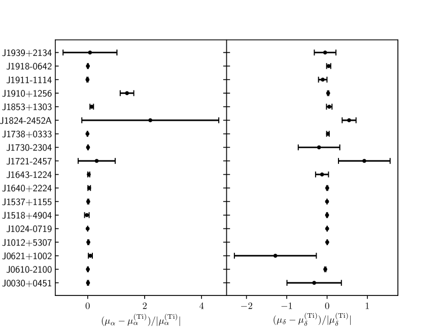
8.6.1 The posterior orbital inclinations and ascending node longitudes
For the four 8P pulsars, orbital inclinations and ascending node longitudes are also inferred alongside the five canonical parameters and (see 8.5.3). The full 8D corner plots out of the 8-parameter inferences are available online5. Prior constraints on and have been provided in 8.5. Owing to bi-modal features of all 1D histograms of , no likelihood component is substantially favored over the other. Hence, no tight posterior constraint on is achieved for any 8P pulsar. Likewise, all 1D histograms of show multi-modal features, which precludes stringent constraints on .
8.6.2 Comparison with Gaia results
From the Gaia Data Release 2 (Gaia-Collaboration18a), Gaia counterparts for pulsars with optically bright companions have been identified and studied by Jennings18; Mingarelli18; Antoniadis21. In the sample, PSR J10125307 and PSR J10240719 have secure Gaia counterparts, while PSR J19101256 has a proposed Gaia counterpart candidate (Mingarelli18). In 8.7, we updated the Gaia results for these three Gaia sources to the Gaia Data Release 3 (DR3, Gaia Collaboration et al. A&A in press).
For PSR J10240719, the Gaia proper motion {, } and parallax are highly consistent with the VLBI+timing ones, which further strengthens the proposal that PSR J10240719 is in an ultra-wide orbit with a companion star (Bassa16; Kaplan16, also see 8.7.2 and 8.8.2). The Gaia proper motion and parallax of PSR J10125307 is largely consistent with the VLBI+timing counterparts. The discrepancy between and and the respective VLBI+timing counterparts can be explained by non-optimal goodness of (Gaia astrometric) fitting (GoF) (see 8.7). On the other hand, the Gaia counterpart candidate for PSR J19101256 (proposed by Mingarelli18) possesses a 4 discrepant from the VLBI+timing one. Though this discrepancy is discounted by the relatively bad GoF by roughly a factor of 1.9 (see 8.7), the connection between the Gaia source and PSR J19101256 remains inconclusive. We note that the parallax zero-points (Lindegren21) of the three Gaia sources are negligible and hence not considered, as is small ( mas, Ding21) compared to the uncertainty of (see 8.7).
| PSR | Gaia DR3 | GoF.∗ | |||
|---|---|---|---|---|---|
| source ID | () | () | (mas) | ||
| J10125307 | 851610861391010944 | 2.7(3) | !-25.9(3) | !1.7(3) | -1.5 |
| J10240719 | 3775277872387310208 | -35.5(3) | -48.35(36) | 0.86(28) | 0.4 |
| J19101256 | 4314046781982561920? | !!!!-2.3(6) | !-6.1(6) | -0.1(8) | 1.9 |
| Sources marked with “?” are tentative Gaia counterpart candidates. | |||||
| Values marked with “!”s are offset from the VLBI+timing counterparts | |||||
| ∗ Goodness of fitting, a parameter (of Gaia data releases) approximately following | |||||
| distribution. A GoF closer to zero indicates better fitting performance. | |||||
8.7 Distances and Space velocities
In this section, we derive pulsar distances from parallaxes (see 8.6), and compare them to the dispersion-measure-based distances. Incorporating the proper motions (see 8.6), we infer the transverse space velocity (i.e., the velocity with respect to the stellar neighbourhood) for each pulsar, in an effort to enrich the sample of 40 MSPs with precise (Hobbs05; Gonzalez11) and refine the distributions of MSP subgroups such as binary MSPs and solitary MSPs.
8.7.1 Parallax-based distances
Inferring a source distance from a measured parallax requires assumptions about the source properties, for which a simple inversion implicitly makes unphysical assumptions (e.g. Bailer-Jones21). Various works (e.g. Lutz73; Verbiest12; Bailer-Jones15; Igoshev16) have contributed to developing and consolidating the mathematical formalism of parallax-based distance inference, which we briefly recapitulate as follows, in order to facilitate comprehension and ready the mathematical formalism for further discussion.
A parallax-based distance can be approached from the conditional probability density function (PDF)
| (8.7) |
where and stands for Galactic longitude and latitude, respectively; . The first term on the right takes the form of
| (8.8) |
assuming is Gaussian-distributed, or more specifically, . The second term on the right side of 8.7 can be approximated as , when the parent population of the target celestial body is uniformly distributed spatially (Lutz73). Given a postulated (Galactic) spatial distribution of , . Hence,
| (8.9) |
We join Verbiest12 and Jennings18 to adopt the (of the “Model C”) determined by Lorimer06a for Galactic pulsars. While calculating the with Equations 10 and 11 of Lorimer06a, we follow Verbiest12 and Jennings18 to increase the scale height (i.e., the parameter “” of Lorimer06a) to 0.5 kpc to accommodate the MSP population. In addition, the distance to the Galactic centre (GC) in Equation 10 of Lorimer06a is updated to kpc (Gravity-Collaboration18). We do not follow Verbiest12; Igoshev16 to use pulsar radio fluxes to constrain pulsar distances, as pulsar luminosity is relatively poorly constrained.
Using the aforementioned mathematical formalism, we calculated for each pulsar, and integrated it into the cumulative distribution function (CDF) . The and is plotted for each pulsar and made available online5. An example of these plots are presented in 8.5. The median distances corresponding to are taken as the pulsar distances, and summarized in 8.6. The distances matching and are respectively used as the lower and upper bound of the 1 uncertainty interval.
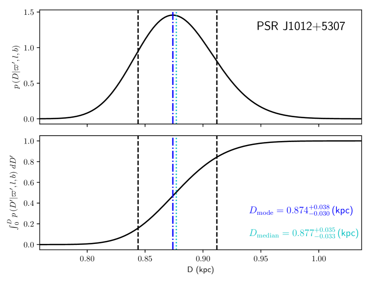
Comparison with DM distances
As mentioned in 8.2.2, the precise DM measured from a pulsar can be used to assess the pulsar distance, provided an model. Using pygedm999https://github.com/FRBs/pygedm, we compile into 8.6 the DM distances (i.e., and ) of each pulsar based on the two latest realisations of model — the NE2001 model (Cordes02) and the YMW16 model (Yao17). For all the DM distances, we adopt typical 20% fractional uncertainties. We have obtained significant () parallax-based distances for 15 out of 18 pulsars. These distances enable an independent quality check of both models.
As is shown with 8.6 and illustrated by 8.6, among the 15 pulsars with parallax-based distance measurements, YMW16 is more accurate than NE2001 in three cases (i.e., PSR J10125307, PSR J16431224 and PSR J19392134), but turns out to be the other way around in four cases (i.e. PSR J06211002, PSR J18531303, PSR J19101256 and PSR J19180642). In other 8 cases, the cannot discriminate between the two models. The small sample of 15 measurements shows that NE2001 and YMW16 remain comparable in terms of outliers. In 2 (out of the 15) cases (i.e., PSR J06102100, PSR J10240719), is about and away from either DM distance, which reveals the need to further refine the models. Such a refinement can be achieved with improved pulsar distances including the ones determined in this work.
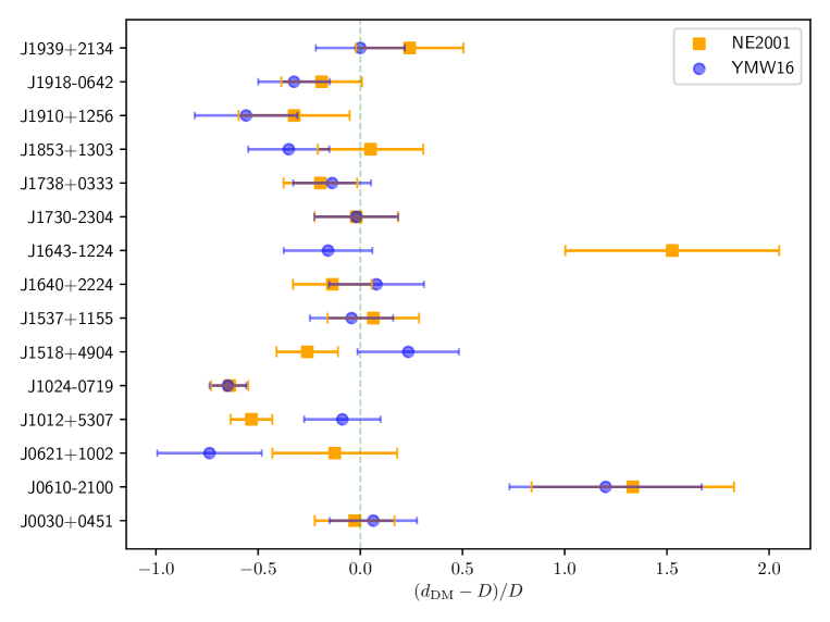
8.7.2 Transverse space velocities
Having determined the parallax-based distances and the proper motions , we proceed to calculate transverse space velocities for each pulsar, namely the transverse velocity with respect to the neighbouring star field of the pulsar. In estimating the transverse velocity of a pulsar neighbourhood, we assume the neighbourhood observes circular motion about the axis connecting the North and South Galactic Poles, which is roughly valid given that all pulsars with significant () share a median of 0.3 kpc. Using the Galactic rotation curve from Reid19 and the full circular velocity of the Sun , we derived the apparent transverse velocity of the neighbourhood , thus obtaining by subtracting the apparent transverse velocity of the pulsar by . Here, the full circular velocity (denoted as in Reid19) is calculated with kpc (Gravity-Collaboration18) and the proper motion of Sgr from Reid19.
To estimate the uncertainty of , we simulated a chain of 50,000 distances for each pulsar based on the that we have obtained in 8.7.1. Besides, we also acquired chains of 50,000 and given the VLBI+timing proper motions of 8.6, assuming and follow Gaussian distributions. With these chains of , and , we calculated 50,000 values, which form a PDF of for each pulsar. The inferred from the PDFs are summarized in 8.6.
In 8.7, we illustrate the in relation to for 16 pulsars with precise distance estimates. Among the 16 pulsars, only PSR J18242452A does not have a significant parallax-based distance. Nevertheless, its can be inferred by incorporating its proper motion with the astrometric information (i.e., distance and proper motion) of its host globular cluster (see 8.9.9). No clear correlation is revealed between and , which reinforces our decision to treat all pulsars across the kpc regime equally. By concatenating the simulated chains, we acquired the PDF for the 16 MSPs (see 8.7), which gives .
Amongst the sources, PSR J10240719 is an obvious outlier, with a velocity of 300 km s-2 that is 3 above the mean. As proposed by Bassa16 and Kaplan16, PSR J10240719 is theorized to have been ejected from a dense stellar region, thus possibly following a different distribution from typical field MSPs (isolated along with their respective companions throughout their lives). In this regard, we turn our attention to the binary sample of pulsars with well determined orbital periods (see of 8.3), and obtain for field binary MSPs. Based on this small sample, we do not find the of the three solitary MSPs (i.e., PSR J00300451, PSR J17302304 and PSR J19392134) to be inconsistent with . Neither are the two DNSs (i.e., PSR J15184904 and PSR J15371155). If we exclude the two DNSs from the binary sample, we would come to for the pulsars with WD companions, which is highly consistent with and .
Compared to previously estimated for a sample of MSPs (Gonzalez11), our is largely consistent but on the smaller side. Boodram22 recently shows that MSP space velocities have to be near zero to explain the Galactic Centre -ray excess (e.g. Abazajian12). Interestingly, the PDF based on our small sample of 16 shows a multi-modal feature, with the lowest mode consistent with zero. Specifically, the 7 pulsars with the smallest share an equally weighted mean of only 25 , which suggests MSPs with extremely low space velocities are not uncommon. Accordingly, we suspect the MSP origin of the GC -ray excess can still not be ruled out based on our sample of .
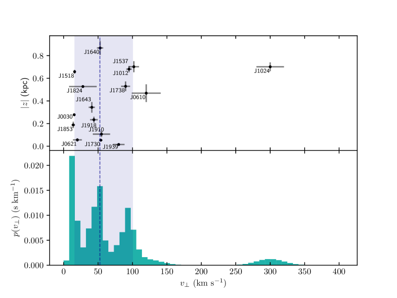
8.8 Radial accelerations of pulsars and orbital-decay tests of gravitational theories
As described in 8.2.2, VLBI astrometry of pulsars, in conjunction with pulsar timing, can enhance the orbital-decay tests of gravitational theories. For binary systems involved in this work, the observed orbital decay has three significant components:
| (8.10) |
where reflects the effect of gravitational-wave damping intrinsic to a binary system, while and are both extrinsic contributions caused, respectively, by relative line-of-sight accelerations (of pulsars) and . Specifically, (where ) is the radial acceleration caused by the tangential motion of pulsars (Shklovskii70), which becomes increasingly crucial for pulsars with larger (e.g. PSR J15371155, Ding21a), as . On the other hand,
| (8.11) |
is a consequence of the gravitational pull (or push) exerted by the Galaxy. Here, and are, respectively, the Galactic gravitational potential (as a function of Galactic position ) and the unit vector in the Earth-to-pulsar direction.
In order to test any theoretical prediction of , it is necessary to estimate and and remove their effect on . Besides this impact, the radial accelerations and would, more generally, affect the time derivative of all periodicities intrinsic to a pulsar system, which include the pulsar spin period derivative . Similar to and , and (where stands for the spin period of a pulsar). As MSPs consist of nearly half of the -ray pulsar population, determining the extrinsic terms of and the intrinsic spin period derivative is essential for exploring the “death line” (i.e., the lower limit) of high-energy emissions from pulsars (e.g. Guillemot16). In 8.8.1 and 8.8.2, we evaluate and one after another. The evaluation only covers pulsars with significant , as both and are distance-dependent.
8.8.1 Shklovkii effects
We estimate the model-independent in a way similar to the estimation of (see 8.7.2). Three chains of 50,000 , and were simulated from their respective PDFs. Using the relation , 50,000 were calculated to assemble the PDF of for each pulsar with significant . The inferred from the PDFs are compiled in 8.8 along with their resultant and .
| PSR | ||||||||||||
| () ∗ | () | (ms) | () ∗ | () | () | () | () | () ∗ | () | () | () | |
| J00300451 | 9.1(2) | -33.0(3.7) | 4.87 | 0.148(3) | -0.54(6) | 10.2 | 10.59(6) | — | — | — | — | — |
| J06102100 | -9(2) | 3.86 | -0.12(3) | 12.3 a | 7.4(9) | -0.72(17) | a | -101(31) | a | |||
| J06211002 | 23.8(4.5) | 28.85 | 2.3(4) | 47.3 | 43.7(6) | 57(11) | — | — | — | |||
| J10125307 | -23.5(2.4) | 5.26 | 7.3(3) | -0.41(4) | 17.1 | 10.2(3) | 73(3) | -4.1(4) | 61(4) | -7.9(5.0) | -13(1) b | |
| J10240719 | -40(3) | 5.16 | 48(3) | -0.69(5) | 18.6 | -29(3) ∗∗ | — | — | — | — | — | |
| J15184904 | 43(1) | -48.5(3.2) | 40.93 | 5.9(2) | -6.6(4) | 27.2 | 27.9(5) | 107(3) | -120(8) | e | ||
| J15371155 | -42(3) | 37.90 | -5.3(4) | 2422.5 | 2372(4) | -5.1(4) | -136.6(3) | -185(4) | -192.45(6) c | |||
| J16402224 | -48.5(4.3) | 3.16 | 1.4(1) | -0.51(5) | 2.8 | 1.9(1) | — | — | — | |||
| J16431224 | 1.0(1.7) | 4.62 | 18.5 | 17.95(7) | 41(72) | — | — | — | ||||
| J17302304 | 11.7(9) | 8.12 | 4.3(2) | 0.32(2) | 20.2 | 15.6(2) | — | — | — | — | — | |
| J17380333 | -6.2(1.6) | 5.85 | -0.12(3) | 24.1 | 22.4(2) | -0.64(16) | -17(3) | -26.1(3.1) | d | |||
| J18531303 | -16(5) | 4.09 | -0.22(7) | 8.7 | 8.69(8) | — | — | — | ||||
| J19101256 | -35(17) | 4.98 | -0.6(3) | 9.7 | 8.3(6) | — | — | — | ||||
| J19180642 | 6.8(1.5) | 7.65 | 0.17(4) | 25.7 | 23.1(3) | 21(5) | — | — | — | |||
| J19392134 | -60(10) | 1.56 | -0.31(5) | 105.1 | 105.41(5) | — | — | — | — | — | ||
| Unless otherwise specified, we adopted , , and from the ATNF Pulsar Catalogue2. | ||||||||||||
| Other references: avan-der-Wateren22; bDing20 and references therein; cDing21a and references therein; dFreire12; eJanssen08. | ||||||||||||
| ∗ “zs” means zeptosecond, which is s. Besides, “pm” and “fs” represent m and s, respectively. | ||||||||||||
| ∗∗ The negative is the result of the radial acceleration caused by a far-away companion (Bassa16; Kaplan16). | ||||||||||||
8.8.2 Relative radial accelerations due to Galactic gravitational pull
We estimate in the same way as Ding21a, following the pioneering work of Zhu19. To briefly demonstrate this method, we present, in 8.9, the based on five different models for the 15 pulsars with significant measurements. The five models are denoted as NT95 (Nice95), DB98 (Dehnen98), BT08 (Binney11), P14 (Piffl14) and M17 (McMillan17) in this paper. The results obtained with NT95, which uses a simple analytical approach, are frequently discrepant compared to the other 4 models. Accordingly, and following Ding21a, we exclude it and use the remaining 4 models to derive the estimate for and its uncertainty, which we present in 8.8 (along with and ).
Incorporating the derived in 8.8.1, we calculated the intrinsic spin period derivative . We note that the negative of PSR J10240719 is probably the consequence of radial acceleration induced by a putative companion in an extremely wide orbit with PSR J10240719 (Bassa16; Kaplan16, also see 8.6.2). In addition to , are estimated for four pulsar systems with reported . The improved PSR J17380333 parallax as well as the re-assessed PSR J10125307 parallax calls for an update to the constraint on alternative theories of gravity (e.g. Freire12; Zhu19; Ding20), which is discussed in 8.8.3.
While performing the analysis, we found an error in the code that had been used to implement the calculation of 8.11 for the Ding21a work (which, to be clear, is not an error in the GalPot101010https://github.com/PaulMcMillan-Astro/GalPot package that provides the models). Therefore, we note that the of PSR J15371155 in 8.8 is a correction to the Ding21a counterpart. Further discussions on PSR J15371155 can be found in 8.9.3.
Last but not least, assuming GR is correct, the approach taken above can be inverted to infer , which can be used to constrain Galactic parameters for the local environment (of the Solar system) (Bovy20), or probe the Galactic dark matter distribution in the long run (Phillips21). The for the three viable pulsars are listed in 8.9.
| PSR | ∗ | |||||
| () | () | () | () | () | () | |
| J00300451 | -29(3) | !-37.0(2) | !-27.3(2) | -35.3(2) | -32.5(3) | — |
| J06102100 | !-12(1) | ! | — | |||
| J06211002 | 24(4) | 23(5) | 24(5) | 24(5) | 25(5) | — |
| J10125307 | !!!-32.0(6) | -24.0(2) | !-19.44(9) | -24.80(9) | -25.80(6) | 05(29) |
| J10240719 | !-45.1(9) | -38.5(6) | !-35.6(9) | -42(1) | -43(1) | — |
| J15184904 | -47.5(5) | -48.1(5) | !-44.8(7) | -50.4(7) | !-51.9(7) | — |
| J15371155 | !!!!-29(1) | -42(1) | -39(2) | -43(2) | -45(2) | |
| J16402224 | !!!-33(1) | -46(3) | -45(3) | -50(3) | -52(4) | — |
| J16431224 | !!10(3) | ! | ! | — | ||
| J17302304 | 13.2(8) | 10.8(6) | 12.1(6) | 11.5(6) | 12.5(7) | — |
| J17380333 | !!!!!!10.1(1.8) | 9(35) | ||||
| J18531303 | -13(3) | — | ||||
| J19101256 | -35(13) | — | ||||
| J19180642 | !!14(2) | 5.9(5) | !8.7(5) | !5.0(2) | 7.4(3) | — |
| J19392134 | -64(8) | -53(8) | -56(8) | -67(9) | -63(9) | — |
| NT95, DB98, BT08, P14 and M17 refer to five different models (see 8.8.2 for | ||||||
| the references). | ||||||
| The “!”s indicate, in the same way as 8.6, the significance of the offset between the | ||||||
| in 8.8 and that of each model. | ||||||
| ∗ is based on the assumption that GR is correct. | ||||||
8.8.3 New constraints on alternative theories of gravity
In the GR framework, the excess orbital decay is expected to agree with zero. However, some alternative theories of gravity expect otherwise due to their predictions of non-zero dipole gravitational radiation and time-varying Newton’s gravitational constant . Both phenomena are prohibited by GR. Namely, in GR, the dipole gravitational radiation coupling constant , and . The large asymmetry of gravitational binding energy of pulsar-WD systems makes them ideal testbeds for dipole gravitational emissions (e.g. Eardley75). In an effort to test (and possibly eliminate) alternative theories of gravity, increasingly tight constraints on and have been placed using multiple pulsar-WD systems (Deller08; Freire12; Zhu19; Ding20).
With the reassessed astrometric results of PSR J10125307, the of PSR J10125307 changes from in Ding20 to . This change is mainly caused by three reasons: 1) priors are placed on the proper motion during inference in this work (but not in Ding20); 2) a Bayesian framework is applied in this work (while Ding20 reported bootstrap results); 3) this work adopts PDF medians as the estimates (while Ding20 used PDF modes). Though barely affecting this work (see 8.5), the choice between PDF mode and median makes a difference to Ding20 given that their parallax PDF is more skewed (see Figure 4 of Ding20). After employing the new VLBI+timing distance, the of PSR J17380333 has shifted from (Freire12) to . More discussions on PSR J17380333 can be found in 8.9.8.
With the new of PSR J10125307 and PSR J17380333, we updated the constraints on and in exactly the same way as Ding20. The prerequisites of this inference are reproduced in 8.10, where the two underlined are the only difference from the Table 6 of Ding20. We obtained
| (8.12) |
Compared to Ding20, becomes more consistent with zero, while the new uncertainties of and remain at the same level.
| PSR | |||||
|---|---|---|---|---|---|
| (d) | () | () | () | ||
| J04374715 | 5.74 | 12(32) | 1.44(7) | 0.224(7) | — |
| J10125307 | 0.60 | 5.1(5.1) | — | 0.174(11) | 10.44(11) |
| J17130747 | 67.83 | 30(150) | 1.33(10) | 0.290(11) | — |
| J17380333 | 0.35 | 1.6(3.5) | 1.46(6) | — | 8.1(2) |
| , and stand for, respectively, pulsar mass, companion mass and | |||||
| mass ratio (i.e., ). See Ding20 for their references. | |||||
8.9 Individual pulsars
In this section, we discuss the impacts of the new astrometric measurements (particularly the new distances) on the scientific studies around individual pulsars. Accordingly, special attention is paid to the cases where there is no published timing parallax . In addition, we also look into the two pulsars (i.e. PSR J17212457 and PSR J18242452A) that have consistent with zero, in an effort to understand the causes of parallax non-detection.
8.9.1 PSR J06102100
PSR J06102100 is the third black widow pulsar discovered (Burgay06), which is in a 7-hr orbit with an extremely low-mass ( , Pallanca12) star. Adopting a distance of around 2.2 kpc, van-der-Wateren22 obtained a -ray emission efficiency in the range of 0.5–3.7, where and are, respectively, the intrinsic NS spin-down power and the -ray flux above 100 MeV.
In addition, van-der-Wateren22 estimated a mass function
| (8.13) |
of for the PSR J06102100 system (where ). Besides, they determined the irradiation temperature (of the companion) K as well as the projected orbital semi-major axis lt-s. Combining these three estimates, we calculated the heating luminosity
| (8.14) |
where represents the Stefan-Boltzmann constant.
Our new distance kpc to PSR J06102100 is less than half the DM-based distances (see 8.6), and significantly below that assumed by van-der-Wateren22. Assuming a NS moment of inertia , the of PSR J06102100 (see 8.8) corresponds to an intrinsic spin-down power
| (8.15) |
of , which is roughly twice as large as the range calculated by van-der-Wateren22. In conjunction with a smaller -ray luminosity (due to closer distance), the reduced to around 0.37 (from estimated by van-der-Wateren22), disfavoring unusually high -ray beaming towards us. Moreover, the heating efficiency drops to (from evaluated by van-der-Wateren22), disfavoring the scenario where the NS radiation is strongly beamed towards the companion.
On the DM discrepancy
In 8.7.1, we noted that our VLBI parallax-derived distance and the DM model-inferred distance to this pulsar differed substantially. Specifically, PSR J06102100 has a measured pc cm-3 while the NE2001 model predicts 27.5 pc cm-3 for a line of sight of length 1.5 kpc. We attribute this discrepancy to thermal plasma or “free electrons” along the line of sight that is not captured fully by a “clump” in the NE2001 model. The NE2001 model includes this “clump” to describe the effects due to the Mon R2 H II region, centered at a Galactic longitude and latitude of (214∘, -12.6∘), located at an approximate distance of kpc (Herbst75). However, the WHAM survey shows considerable H in this direction, extending over tens of degrees. Lines of sight close to the pulsar show changes in the H intensity by factors of two, but an approximate value toward the pulsar is roughly 13 Rayleighs, equivalent to an emission measure pc cm-6 (for a temperature K). Using standard expressions, as provided in the NE2001 model, to convert EM to DM, there is sufficient H intensity along the line of sight to account for the excess DM that we infer from the difference between our parallax-derived distance and the NE2001 model distance.
8.9.2 PSR J15184904
The 41-ms PSR J15184904, discovered by Sayer97, is one of the only two DNSs in the current sample. According to Janssen08, the non-detection of Shapiro delay effects suggests at 99% confidence level. Accordingly, we adopted 0.73 as the upper limit of , and carried out 8-parameter Bayesian inference, which led to a bi-modal posterior PDF on and a multi-modal PDF on (see the online corner plot5). The predominant constraints on both and come from the measurement (Janssen08 or see 8.4). Though there are 3 major likelihood peaks for the , two of them gather around 171∘, making the PDF relatively more concentrated. When a much more precise measurement is reached with new timing observations, the existing VLBI data will likely place useful constraints on and . So will additional VLBI observations.
In addition to and , the 8-parameter Bayesian inference also renders a parallax , which becomes the most significant parallax achieved for a DNS. In contrast, to detect a timing parallax for PSR J15184904 would take years (Janssen08), due to its relatively high ecliptic latitude of 63∘.
8.9.3 PSR J15371155
PSR J15371155, also known as PSR B153412, is the second discovered DNS (Wolszczan91). The DNS displays an exceptionally high proper motion amongst all Galactic DNSs (see Table 3 of Tauris17), leading to an unusually large Shklovskii contribution to observed timing parameters. Therefore, precise astrometry of the DNS plays an essential role in its orbital decay test of GR. The most precise astrometric parameters of PSR J15371155 are provided by Ding21a based on the same dataset used in this work, which result in . Subsequently, Ding21a estimated , and concluded .
In this work, we inferred on top of the canonical astrometric parameters, which is the only difference from the Bayesian method of Ding21a. Despite this difference, our astrometric results of PSR J15371155 remain almost the same as Ding21a. So is our re-derived . However, as is mentioned in 8.8.2, the estimated by Ding20c is incorrect due to a coding error. After correction, drops to (see 8.8). Consequently, we obtained .
As Ding21a have pointed out, the limiting factor of the GR orbital decay test using PSR J15371155 remains the distance precision, which generally improves as with additional observations, but can be accelerated if more sensitive instrumentation can be deployed. On the other hand, the extremely high braking index of 157 (two orders higher than the normal level) calculated from the rotational frequency , its first derivative and its second derivative (Fonseca14) indicate likely timing noise contributions that may affect the observed orbital period derivative to some degree. This will be clarified with continued timing observations and refined timing analysis.
8.9.4 PSR J16402224
PSR J16402224 is a 3.2-ms MSP (Foster95) in a wide ( d) orbit with a WD companion (Lundgren96). The results for PSR J16402224 have been published in Vigeland18, which are highly consistent with our re-assessed quasi-VLBI-only results (see Table 2 of Vigeland18 and 8.5). Our 8-parameter Bayesian inference renders a 1D histogram of with 4 likelihood components at 0∘, 140∘, 200∘ and 320∘, which is predominantly shaped by the prior on from pulsar timing (see 8.4).
8.9.5 PSR J16431224
PSR J16431224 is a 4.6-ms pulsar in a 147-d orbit with a WD companion (Lorimer95a). As a result of multi-path propagation due to inhomogeneities in the ionised interstellar medium (IISM), the pulse profiles of PSR J16431224 are temporally broadened (e.g. Lentati17). As the Earth-to-pulsar sightline moves through inhomogeneous scattering “screen(s)” (in the IISM), the temporal broadening varies with time; at 1 GHz, fluctuates up and down by s on a yearly time scale (Lentati17). Meanwhile, the moving scattering “screen(s)” would also change the radio brightness of the pulsar. This effect, as known as pulsar scintillation, is used to constrain the properties of both PSR J16431224 and the scattering screen(s) between the Earth and the pulsar (Mall22). The scintillation of PSR J16431224 has previously been modelled with both isotropic and anisotropic screens (Mall22). The isotropic model renders a pulsar distance kpc and locates the main scattering screen at kpc; in comparison, the anisotropic model yields a pulsar distance kpc, and necessitates a secondary scattering screen kpc away (from the Earth) in addition to a main scattering screen at kpc distance (Mall22). On the other hand, the HII region Sh 2-27 in front of PSR J16431224 is suspected to be associated with the main scattering screen of the pulsar. This postulated association is strengthened by the agreement between the distance to the main scattering screen (based on the two-screen anisotropic model, Mall22) and the distance to the HII region (i.e., pc, Ocker20).
Independent check on the postulated association between the HII region Sh 2-27 and the main scattering screen
Besides the pulse broadening effect, the scattering by the IISM would lead to apparent angular broadening of the pulsar, which has been detected with VLBI at GHz (e.g. Bower14). By the method outlined in Appendix A of Ding20c, we measured a semi-angular-broadened size mas for PSR J16431224, which is the only significant determination in the catalogue. Likewise, the secondary in-beam calibrator of PSR J16431224 is also scatter-broadened, which may likely introduce additional astrometric uncertainties (see more explanation in 8.9.6).
As both pulse broadening and angular broadening are caused by the IISM deflection, , , the pulsar distance , and the distance(s) to the scattering screen(s) are geometrically related. Assuming there is one dominant thin scattering screen, we make use of following approximate relation
| (8.16) |
where stands for the speed of light in vacuum.
To estimate the unknown at our observing frequency of 1.55 GHz, we used the data spanning MJD 54900—57500 from the PPTA second data release (Kerr20). We analysed the dynamic spectra of observations centred around 3.1 GHz and recorded with the PDFB4 processor, using the scintools111111https://github.com/danielreardon/scintools package (Reardon20). A model was fit to the auto-correlation function of each dynamic spectrum, which has an exponential decay with frequency (Reardon19). The characteristic scintillation scale (in frequency) is related to the scattering timescale with . We found the mean temporal broadening ns at 3.1 GHz, with fluctuations of ns (see 8.8). To convert this to our observing frequency 1.55 GHz, we compare the maximum degree (i.e., 60 ns) of fluctuations at 3.1 GHz to that (i.e., s, Lentati17) at 1 GHz, and acquired an indicative scaling relation
| (8.17) |
where is the observing frequency. This relation reasonably agrees with the scaling relation associated with the Kolmogorov turbulence (e.g. Armstrong95). With the indicative scaling relation, we calculated s. It is timely to note that (on the left side of 8.16) is frequency-independent. By combining 8.16 and 8.17, we come to another equivalent indicative scaling relation
| (8.18) |
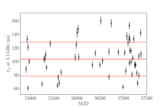
Substituting s, mas and kpc into 8.16, we obtained pc, where the uncertainty is derived with a Monte-Carlo simulation. This is consistent with the distance to the HII region Sh 2-27 (Ocker20), hence independently supporting the association between the HII region and the main scattering screen of PSR J16431224.
Probing scintillation models
Apart from the above check on the connection between the HII region Sh 2-27 and the main scattering screen, the angular broadening of PSR J16431224 also promises a test of the aforementioned isotropic scintillation model proposed by Mall22. To do so, we changed the pulsar distance to the one inferred with the model (i.e., kpc). With this change, we derive pc, which disagrees with kpc based on the isotropic model. To investigate the impact of a different scaling relation , we inferred s with both and based on the isotropic model (Mall22), which corresponds to an unreasonably large . Hence, we conclude that our and cannot easily reconcile with the one-screen isotropic model proposed by Mall22.
Fundamentally, the irreconcilability implies a one-screen model might be incapable of describing both scintillation and angular broadening effects of PSR J16431224. In principle, it is possible to analyse a multi-screen model with a series (at various time ) and its associated , instead of only using their mean values. However, this analysis is not feasible for this work, as and were not measured on the same days. Nonetheless, we can still investigate whether our observations of PSR J16431224 can reconcile with the scintillation observations (Mall22) in the context of a two-screen model.
In the scenario of two thin scattering screens, we derived the more complicated relation
| (8.19) |
where and are the distance to the first and the second scattering screen, respectively; represents a half of the opening angle of the second scattering screen (closer to the pulsar) as seen from the pulsar. As a side note, 8.16 can be considered a special case (i.e., ) of 8.19. In 8.19, all parameters except are known, either determined with the anisotropic two-screen model or obtained in this work. Hence, it is feasible to constrain the geometric parameter with the known parameters.
However, 8.19 can yield unphysical solutions (i.e., ). We applied the simple condition
| (8.20) |
to ensure 8.19 gives physical solutions of . This equation is equivalent to , where corresponds to the one-screen solution of 8.16. This is because would always lead to longer routes, thus exceeding the budget. It is important to note that 8.20 is valid for a model with any number of scattering screens. Hence, we recommend to use 8.20 in scintillation model inferences as a prior condition, to cater for the constraints imposed by and (and thereby truncate the parameter space of a scintillation model).
To test the anisotropic two-screen model (Mall22) with our and , we calculated pc with the pulsar distance (i.e., kpc) based on the anisotropic two-screen model. This is consistent with pc (Mall22) (therefore not ruling out ). That is to say, our and measurements can loosely reconcile with the anisotropic two-screen model (Mall22). In comparison, we reiterate our finding that a one-screen model is difficult to describe both scintillation and angular broadening effects of PSR J16431224.
8.9.6 PSR J17212457
PSR J17212457 is a 3.5-ms solitary MSP discovered at intermediate Galactic latitudes Edwards01. The main secondary phase calibrator of PSR J17212457 (and indeed, all the sources near it on the plane of the sky) is heavily resolved due to IISM scattering, which leads to non-detections on the longest baselines and a lack of calibration solutions for some antennas, reducing the spatial resolution of the VLBI observations. The non-uniform IISM distribution also leads to refractive image wander as the line-of-sight to the pulsar changes (e.g., Kramer21a), which is most pronounced for heavily scatter-broadened sources such as the calibrator for PSR J17212457 . In conjunction with the lower spatial resolutions, which reduces positional precision to begin with, this additional noise term likely results in the parallax non-detection (see 8.5).
8.9.7 PSR J17302304
PSR J17302304 is a solitary pulsar spinning at ms (Lorimer95a). Being so far the least-energetic (in terms of ) -ray pulsar (Guillemot16), the pulsar plays a key role in exploring the death line of NS high-energy radiation. Substituting and of 8.15 with values listed in 8.8, we substantially refined the death line (of all -ray-emitting pulsars) to
| (8.21) |
which is consistent with (but on the higher side of) the previous estimate by Guillemot16 (assuming the same ). On the other hand, we updated the -ray luminosity (above 100 MeV) to , where the precision is limited by the less precise (Guillemot16). Accordingly, we obtained .
8.9.8 PSR J17380333
PSR J17380333, discovered from a 1.4-GHz high-Galactic-latitude survey with the 64-m Parkes radio telescope (Jacoby09), is a 5.85-ms pulsar in a 8.5-hr orbit with a WD companion. Thanks to the relatively short , the WD-pulsar system plays a leading role in constraining alternative gravitational theories that predict dipole gravitational radiation (Freire12; Zhu15).
Our VLBI-only is away from the most precise (see 8.5 and 8.6). After adopting timing priors, mas becomes closer to mas (Freire12), meaning that is only 1.2 times larger than the previous estimate. On the other hand, our re-assessed , based on more realistic models, is smaller than that estimated with the NT95 model (Freire12). Combining the unchanged the re-derived is almost the same as the previous estimate, as the change of happens to nearly cancels out that of .
Future pulsar timing or VLBI investigation into the discrepancy between (Freire12) and is merited by the importance of the pulsar system. Specifically, if the true parallax turns out to be around 0.5 mas, it would not only mean that is 1.4 times higher than the estimate by Freire12, but also suggest the WD radius to be 1.4 larger (as according to Equation 1 of Antoniadis12). A higher would lead to lighter WD and NS (as the mass ratio is well determined), thus smaller .
8.9.9 PSR J18242452A
PSR J18242452A is a 3-ms solitary pulsar discovered in the Globular cluster M28 (NGC 6626) (Lyne87a). The calibration configuration for this pulsar was sub-optimal, as the best in-beam phase calibrator for PSR J18242452A was both resolved and faint (3.3 mJy, see 8.1), leading to noisy solutions, especially on the longest baselines. This is likely responsible for the parallax non-detection (see 8.5), and indicates that higher sensitivity to enable improved calibration solutions would be advantageous in any future VLBI campaign.
The proper motion of M28 is estimated to be and (Vasiliev21) with Gaia Early Data Release 3 (EDR3). Hence, the relative proper motion of PSR J18242452A with respect to M28 is and . Combining the M28 distance kpc estimated by Baumgardt21, we obtained the transverse space velocity for PSR J18242452A, which is smaller than the typical escape velocity ( ) of a globular cluster. Therefore, the pulsar is probably (as expected) bound to M28.
8.10 Summary and Future prospects
In this release paper, we have presented VLBI astrometric results for 18 MSPs, including a re-analysis of three previously published sources. From the 18 sources, we detect significant parallaxes for all but three. For each pulsar, at least one self-calibratable in-beam calibrator was identified to serve as the reference source of relative astrometry. In three cases, 1D interpolation, a more complex observing and data reduction strategy, is adopted to further suppress propagation-related systematic errors. Among the three pulsars, PSR J19392134 is the brightest MSP in the northern hemisphere. Hence, we took one step further to perform inverse-referenced 1D interpolation using PSR J19392134 as the in-beam calibrator. Compared to the pioneering Multi-View study of Rioja17 at 1.6 GHz, the larger number of observations and targets here provides more opportunities to characterise the interpolation performance, which is crucial for ultra-precise astrometric calibration schemes proposed for future VLBI arrays incorporating the Square Kilometre Array (SKA). Based on a small sample of three, we found that has consistently inflated after applying 1D interpolation (see 8.5.1). This inflation implies that the higher-order terms of in the phase screen approximation may not be negligible, and could become the limiting factor of the ultra-precise SKA-based astrometry using the Multi-View strategy. Further investigations of the same nature, especially using temporally simultaneous (in-beam) calibrators, at low observing frequencies are merited and encouraged.
In this paper, we present two sets of astrometric results – the quasi-VLBI-only results (see 8.5) and the VLBI+timing results (see 8.6). Both sets of astrometric results are inferred with the astrometry inference package sterne7. The former set of results is largely independent of any input based on pulsar timing, making use only of orbital parameters as priors in the inference of orbital reflex motion, which affects only four pulsars from our sample and is near-negligible in any case. The latter, however, additionally adopts the latest available timing parallaxes and proper motions as priors of inference wherever possible, affecting all pulsars in our sample. While the latter approach typically gives more precise results, we note that this is dependent on the accuracy of the timing priors, and identify seven pulsars (PSR J06102100, PSR J16431224, PSR J17302304, PSR J17380333, PSR J18242452A, PSR J18531303 and PSR J19101256) for which disagreement between the quasi-VLBI-only and the timing priors mean that the VLBI+timing results should be treated with caution. From the VLBI perspective, we looked into possible causes of additional astrometric uncertainties, including non-optimal calibrator quality (see 8.9.6 and 8.9.9) and calibrator structure evolution (see 8.6). In future, proper motion uncertainties (including any unaccounted systematic error due to calibrator structure evolution) can be greatly reduced with only extra observations per pulsar. For example, a 10-yr time baseline can improve the current VLBI-only proper motion precision by roughly a factor of 8.
From the VLBI+timing parallaxes , we derived distances using 8.9. Incorporating the PDFs of and proper motions {, }, we estimated the transverse space velocities for 16 pulsars with significant distance determination, and found their to be generally on the smaller side of the previous estimates (Hobbs05; Gonzalez11). Boodram22 propose that MSPs must have near-zero space velocities in order to explain the Fermi Galactic centre excess. Our relatively small space velocities inferred for 16 MSPs suggest that MSPs may not be ruled out as the source of the Galactic -ray centre excess. Moreover, smaller space velocities of MSPs would also potentially address the globular cluster retention problem outlined in 1.3.1. If the multi-modal feature of the is confirmed with a sample of MSPs, it may serve as a kinematic evidence for alternative formation channels of MSPs (Bailyn90; Gautam22, also see Ding23a as an analogy).
In addition, we estimated the radial accelerations of pulsars with their distances and proper motions (see 8.8), which allows us to constrain the intrinsic spin period derivative and the intrinsic orbital decay (see 8.8). We used the improved of PSR J17302304 to place a refined upper limit to the death line of -ray pulsars (see 8.9.7), and the (of PSR J10125307 and PSR J17380333) to constrain alternative theories of gravity (see 8.8.3). As already noted by Ding20, the orbital decay tests (of gravitational theories) with the three viable systems (i.e., PSR J10125307, PSR J15371155 and PSR J17380333) will be limited by the distance uncertainties, as parallax precision improves much slower than the precision (Bell96).
Moreover, we detected significant angular broadening of PSR J16431224, which we used to 1) provide an independent check of the postulated connection between the HII region Sh 2-27 and the main scattering screen of PSR J16431224, and 2) test the scintillation models proposed by Mall22. In future scintillation model inferences, angular broadening and temporal broadening measurements, where available, are suggested to be used as priors using 8.20, in order to achieve more reliable (and potentially more precise) scintillation model parameters. Such an inference would also complete the geometric information of the deflection routes (using 8.19, for example, in the two-screen case).
Acknowledgements
The authors thank Y. Kovalev, L. Petrov and N. Wex for useful discussions. HD is supported by the OzGrav scholarship through the Australian Research Council project number CE170100004. PF thanks the continued support by the Max-Planck-Gesellschaft. SC, JMC, EF, DK and TJWL are members of the NANOGrav Physics Frontiers Center, which is supported by NSF award PHY-1430284. This work is based on observations with the Very Long Baseline Array (VLBA), which is operated by the National Radio Astronomy Observatory (NRAO). The NRAO is a facility of the National Science Foundation operated under cooperative agreement by Associated Universities, Inc. Pulsar research at Jodrell Bank Observatory is supported by a consolidated grant from STFC. Pulsar research at UBC is supported by an NSERC Discovery Grant and by the Canadian Institute for Advanced Research. The Nançay Radio Observatory is operated by the Paris Observatory, associated with the French Centre National de la Recherche Scientifique (CNRS). We acknowledge financial support from the “Programme National de Cosmologie et Galaxies” (PNCG) and “Programme National Hautes Energies” (PNHE) of CNRS/INSU, France. The Parkes radio telescope (Murriyang) is part of the Australia Telescope, which is funded by the Commonwealth Government for operation as a National Facility managed by CSIRO. The Wisconsin Mapper and its Sky Survey have been funded primarily by the National Science Foundation. The facility was designed and built with the help of the University of Wisconsin Graduate School, Physical Sciences Lab, and Space Astronomy Lab. NOAO staff at Kitt Peak and Cerro Tololo provided on-site support for its remote operation. Data reduction and analysis was performed on OzSTAR, the Swinburne-based supercomputer. This work made use of the Swinburne University of Technology software correlator, developed as part of the Australian Major National Research Facilities Programme and operated under license. sterne as well as other data analysis involved in this work made use of numpy (Harris20), scipy (Virtanen20), astropy (The-Astropy-Collaboration18) and the bilby package (Ashton19).
Data and Code Availability
-
•
The VLBA data can be downloaded from the NRAO Archive Interface at https://data.nrao.edu with the project codes in 8.1.
-
•
Image models of phase calibrators are provided at https://github.com/dingswin/calibrator_models_for_astrometry.
-
•
Supplementary materials supporting this paper can be found at https://github.com/dingswin/publication_related_materials.
-
•
The data reduction pipeline psrvlbireduce is available at https://github.com/dingswin/psrvlbireduce (version ID: b8ddafd).
-
•
The astrometry inference package sterne can be accessed at https://github.com/dingswin/sterne.
Chapter 9 Conclusion
9.1 Thesis summary
This thesis presents precise astrometric results for three classes of Galactic neutron stars (NSs) — NS X-ray binaries (XRBs), magnetars and recycled pulsars (including double neutron stars and other millisecond pulsars), using either the Very Long Baseline Array (VLBA) or the Gaia space telescope (Gaia-Collaboration16). Observationally, the thesis obtains 15 significant () parallaxes of millisecond pulsars (MSPs) from the project — the largest ever astrometric survey of MSPs (see 8.2.3), and determined the first two magnetar parallaxes including a 5 preliminary parallax for the fastest-spinning magnetar Swift J1818.01607 (see 4.3).
Methodologically, this thesis involves the development of two new packages — the psrvlbireduce111https://github.com/dingswin/psrvlbireduce VLBI data reduction pipeline and the sterne222https://github.com/dingswin/sterne astrometric Bayesian inference package. Using the two packages, the thesis made the first realizations of 1D interpolation (see 3.4.1, 4.3 and 8.4.1), inverse-referenced 1D interpolation (see 8.4.2) and multi-source astrometric inference (see 8.5.1) on pulsars. Based on a small sample of 3 pulsars astrometrically measured using 1D interpolation, the thesis reveals that the higher-order term of interpolation might be non-negligible at 1.5 GHz (see 8.5.1), which may become the limiting factor of the Multi-View observing strategy (Rioja17) designed for the Square Kilometre Array. Additionally, a generic quasar-based method to estimate parallax zero-points is proposed for Gaia astrometry (see 5.4.1).
Using the precise astrometric results, the thesis fulfills abundant scientific motivations (outlined in 1), which are categorized into 4 perspectives. Firstly, based on 16 pulsars with significant distance estimation, a multi-modal transverse space velocity distribution was determined for MSPs (see 8.7.2). One mode of this distribution can be approximated by a normal distribution that is consistent with zero, which may potentially observationally resolve the two retention problems described in 1.3.1 — the globular cluster retention problem (e.g. Pfahl02) and the observed Galactic Centre -ray excess (e.g. Abazajian12; Boodram22). The low mode also agrees with the prediction of alternative MSP and NS formation channels mentioned in 1.3.1. In a similar vein, this thesis proposes to use the distribution of magnetars as the probe of magnetar formation channels (see 4.2). Previous study of magnetar distribution based on a sample of 8 objects has shown a mean of around 150 (Tendulkar13; Lyman22) that is consistent with normal pulsars (Hobbs05). This thesis determined the astrometry of 2 of the 5 constant radio magnetars, and hence increased the sample of magnetars with precise velocities (see 1.3.2), and further confirms the relatively small as opposed to the earlier postulate of Duncan92 (which suggested magnetars might be very high-velocity objects).
Secondly, the significant proper motions and parallaxes measured for pulsars enable precise determination of the extrinsic time derivatives of pulsar spin periods and orbital periods (where applicable) (see 1.5.1 and 1.6). By deducting the extrinsic terms from the observed values, the intrinsic spin period derivatives and intrinsic orbital decays are estimated. The allow precise estimation of the spin-down power (see 1.1.5), which refines the death line of -ray pulsars using PSR J17302304 (see 1.6 and 8.9.7) — the -ray pulsar with the smallest spin-down power (Lorimer95a; Guillemot16). The improves the orbital-decay test of general relativity (GR) with the double neutron star system PSR J15371155 (see 7.5 and 8.9.3), and tightens the constraints on alternative gravitational theories (that predict time variation of the Newton’s gravitational constant and dipolar gravitational radiation) using four pulsar-WD systems (see 6.5.3 and 8.8.3).
Thirdly, 4 photospheric radius expansion (PRE) bursters (explained in 1.6.1 and 5.2) with significant parallaxes from the Gaia Early Data Release 3 (EDR3) are used to refine the PRE burster distances, and constrain the composition of the nuclear fuel accumulated on the NS surface at the time of PRE bursts, assuming that the simplistic PRE model is correct. Furthermore, by relaxing the prior (of Bayesian inference) to include unphysical ranges, the thesis novelly probes the simplistic PRE burst model that has been used to estimate the distances to most PRE bursters (see 5.5.3). It is found that the simplistic PRE burst model largely stands the test by the PRE burster parallaxes, at the Gaia EDR3 parallax uncertainty level.
Last but not least, this thesis also constrains the distribution of ionised interstellar medium (IISM) in different ways. The parallax-based distances of 15 pulsars are used to test the two prevailing models (Cordes02; Yao17) of Galactic free-electron distribution , which shows that the two models have comparable reliability. In addition, the angular-broadened size (see 1.4.2) of PSR J16431224 is precisely determined with VLBA observations at 1.55 GHz. Incorporating a temporal broadening estimate , the 1) independently supports the association between the main scattering screen of PSR J16431224 emission and the HII region Sh 2-27, and 2) favors the two-screen scintillation model over the one-screen one (both proposed by Mall22). Where and are known, the thesis proposes to use 8.20 to restrict the parameter space of viable scintillation models.
9.2 Future prospects
Although a good amount of scientific outputs have been derived from the catalogue (see 9.1), a few further studies promised by the data are not covered by this thesis. Specifically, the solar system ephemerides (SSEs) can be examined using the absolute positions of MSPs (see 1.5.4), which can potentially refine the prior knowledge of SSEs for the BAYESEPHEM framework (Arzoumanian18) or other frameworks of its kind, then improve the pulsar timing array (PTA) sensitivities. This work of SSE examination is underway. The absolute MSP positions will be estimated in the same way as 6.4.2, but based on refined phase calibrator positions determined at 1.5 GHz with a parallel project. This incorporated effort will likely achieve mas precision for each MSP position, enabling the most sensitive SSE examination.
On another line of research, the novel quasar-based method proposed to estimate Gaia parallax zero-points has so far only been used on five sources (see 5.4.1). To increase the statistical importance of the estimation method, future work will optimize the method, and apply it to a larger sample covering both low and high Galactic latitudes , which may further examine the excess (compared to the empirical of Lindegren21) at low found by Ren21 (and supported by Ding21 or 5).
Meanwhile, many of the studies presented in this thesis are limited by their small sample sizes, hence prioritizing increases in the dimension of the astrometric sample. For example, the establishment of a statistically significant magnetar distribution requires dozens of magnetars precisely measured astrometrically. However, only about a dozen magnetars are sufficiently bright at optical/infrared or radio (see the McGill Online Magnetar Catalogue333http://www.physics.mcgill.ca/~pulsar/magnetar/main.html, Olausen14), which limits the sample size of magnetars that can be precisely measured astrometrically. Until very recently, magnetars were believed to be short-lived electromagnetic sources that quickly exhaust their energy sources and become invisible, which is consistent with the small () number of magetars ever identified (Olausen14). Nevertheless, the recent discovery of ultra-long period pulsars (Hurley-Walker22; Caleb22) suggests a potentially previously overlooked radio magnetar population, which may supercharge the investigation of the magnetar distribution that would shed more light on the magnetar formation channels (see 4.2).
Likewise, the tentative multi-modal distribution of MSPs revealed by 16 pulsars merits a larger astrometric survey of MSPs. The multi-modal feature, if confirmed with MSPs carefully and systematically studied astrometrically, would strongly indicate alternative formation channels (Michel87; Bailyn90; Tauris13; Gautam22; Miyaji80, also see 1.3.1). Furthermore, an extended astrometric survey focusing on newly discovered MSPs is essential for the PTA research. As mentioned in 1.5.3, VLBI astrometry of newly discovered MSPs can potentially maximize the pace of PTA sensitivity improvement (Siemens13; Madison13), assuming that the new MSPs are added to the PTA.
As newly discovered MSPs tend to be fainter than historical MSPs (not to mention that MSPs are already generally fainter than canonical pulsars), MSP astrometry would become increasingly limited by the sensitivity of a VLBI array. A high-sensitivity VLBI array, e.g. FAST-VLBI (Zhang17; Chen20), SKA-VLBI (Paragi14) and ngVLA (McKinnon19), would enable precise astrometry of further-away ( kpc) MSPs, which are often more important for refining the model. Alongside the sensitivity improvement is the demand for advanced calibration techniques (see 2.2). Specifically, in-beam phase referencing (see 2.2.1) would be the optimal strategy for FAST-VLBI due to its relatively long slewing time, while the interpolation strategy would be less effective (see 2.2.3). In comparison, interpolation may potentially serve as the standard phase calibration strategy for SKA-VLBI (Rioja17), capitalizing on the beamforming capacity of the SKA (and ideally other components of the SKA-VLBI array). As the parallaxes to be measured get smaller, the calibration techniques have to keep developing.
Apart from the use of high-sensitivity arrays, astrometry spanning a long time (e.g. 3.3) can also greatly improve astrometric precision, especially for the proper motion. This “long-haul” astrometry can be realized with two groups of VLBI observations many years apart. Specifically, the pulsars were astrometrically measured roughly 6 years ago. Adding long-haul VLBI observations per source can substantially reduce the proper motion uncertainties, which may resolve the discrepancy between the VLBI-only and the timing proper motions of some of the pulsars (see 8.6).
To improve the astrometric precision of Gaia sources also requires continued observations. This is particularly important for probing the simplistic PRE model using the Gaia parallaxes of the few PRE bursters (see 5.5.3), but would be ultimately limited by the lifespan of the Gaia mission. In comparison, VLBI astrometry of PRE bursters with relatively frequent outbursts (e.g. Aql X1) would potentially achieve better astrometric precision in the long run, therefore being essential for the study of PRE models.