Pilot Reuse in Cell-Free Massive MIMO Systems: A Diverse Clustering Approach

Abstract

Distributed or Cell-free (CF) massive Multiple-Input, Multiple-Output (mMIMO), has been recently proposed as an answer to the limitations of the current network-centric systems in providing high-rate ubiquitous transmission. The capability of providing uniform service level makes CF mMIMO a potential technology for beyond-5G and 6G networks. The acquisition of accurate Channel State Information (CSI) is critical for different CF mMIMO operations. Hence, an uplink pilot training phase is used to efficiently estimate transmission channels. The number of available orthogonal pilot signals is limited, and reusing these pilots will increase co-pilot interference. This causes an undesirable effect known as pilot contamination that could reduce the system performance. Hence, a proper pilot reuse strategy is needed to mitigate the effects of pilot contamination. In this paper, we formulate pilot assignment in CF mMIMO as a diverse clustering problem and propose an iterative maxima search scheme to solve it. In this approach, we first form the clusters of User Equipments (UEs) so that the intra-cluster diversity maximizes and then assign the same pilots for all UEs in the same cluster. The numerical results show the proposed techniques’ superiority over other methods concerning the achieved uplink and downlink average and per-user data rate.

I Introduction

Distributed or Cell-free (CF) massive Multiple-Input, Multiple-Output (mMIMO) [1, 2, 3, 4, 5, 6, 7] has been considered as one of the potential technologies for beyond-5G (B5G) and 6G wireless networks thanks to its capability of providing relatively uniform service to the User Equipments (UEs) in the coverage area. As the name implies, CF systems, unlike traditional cellular networks, do not consider the concepts of cell or cell boundaries, where a Base Station (BS) serves multiple UEs within its cell coverage. In CF mMIMO, UEs are jointly served by a relatively larger number of geographically distributed Access Points (APs) over the same time-frequency resource. CF mMIMO lies at the intersection of different technologies like mMIMO [8, 9, 10, 11], Coordinated MultiPoint (CoMP) [12, 13] and Ultra Dense Network (UDN) [14, 15], combing the best of each technology, while eliminating their deficiencies [4]. CF mMIMO adopts its physical layer from cellular mMIMO, which brings 10x Spectral Efficiency (SE) improvement over legacy cellular networks [4]. This gain comes from deploying a massive number of antennas at each BS, that provide spatial multiplexing for many UEs by digital beamforming. CF mMIMO is inherently a distributed implementation of co-located mMIMO, where densely developed APs provide service for a smaller number of UEs with a coherent joint transmission and Time Division Duplexing (TDD) operation. The procedure takes place in a user-centric (as opposed to network-centric) fashion, where the UEs are surrounded and served by several APs. The APs are connected to one or multiple central processing units (CPUs), i.e., edge-cloud processors or cloud radio access network (C-RAN) [16] data centers [17], by high-capacity fronthaul links where data precoding/decoding operations, synchronization, and other network management operations take place. The acquisition of accurate Channel State Information (CSI) is critical for different CF mMIMO operations. Hence, it employs Uplink (UL) pilots to estimate the channel at the AP while eliminating the Downlink (DL) pilot training phase by considering channel reciprocity. However, due to the limited number of channel uses in each coherence interval, only a limited number of orthogonal pilots are available, typically smaller than the number of UEs. The number of available pilots is independent of the number of UEs and is limited due to the natural channel variation in the time and frequency domains [18]. Hence, reusing the same pilot for different UEs is inevitable, which introduces undesirable effects known as pilot contamination: due to the co-pilot interference among UEs, the fading channel at the APs can not be accurately estimated.

I-A Related Works

Different pilot assignment strategies have already been proposed in the literature to solve this issue. The most straightforward approach is random pilot assignment [2], where each AP independently assigns a random pilot to its associated UEs. This is a fully distributed procedure and requires a minimum degree of centralization and knowledge of the pilots of other UEs, but has the worst performance among different pilot reuse strategies. Hence, a better pilot assignment policy needs to know other UEs’ (at least its neighbors) pilots to reduce the effects of pilot contamination. A greedy pilot assignment is proposed in [2], that iteratively updates the pilot of the UE with minimum rate. A structured pilot assignment scheme is proposed in [19], that maximizes the minimum distance of the co-pilot UEs. The location information of the UEs is utilized in location-based greedy pilot assignment [20] to improve the initial pilot assignment. The pilot assignment is also considered as an interference management problem with multiple group-casting messages in [21] and then solved by topological pilot assignments where both known and unknown UE/AP connectivity patterns are considered.

Graph theory has also been used to model pilot assignment in CF mMIMO, where graph coloring [22] and weight graphic [23] schemes created and employed an interference graph to assign pilots to different UEs. The authors in [24, 25] used tabu search pilot assignment in CF mMIMO. Pilot assignment can also be considered as a graph matching problem and then solved by the Hungarian algorithm [26]. A weighted count-based pilot assignment is presented in [27], that uses the UEs prior geographic information and pilot power to maximize the pilot reuse weighted distance. A scalable pilot assignment scheme is presented in [28] to grant massive access in CF mMIMO. Another scalable pilot assignment algorithm based on deep learning is presented in [29], that uses UEs geographical locations as an input. The authors in [30] presented a pursuit learning approach for joint pilot allocation and AP association. A pilot assignment strategy based on quantum bacterial foraging optimization is proposed in [31]. The pilot assignment is also considered as a balanced diverse clustering problem in [32] and solved by a repulsive clustering approach.

I-B Motivation and Contributions

The co-pilot interference, in principle, is caused by pilot reuse for similar UEs, i.e., in terms of geographical proximity and/or similar channel coefficient. Hence, an intelligent pilot assignment scheme could employ the similarity information to avoid pilot reuse for similar UEs. Motivated by this consideration, in this paper, we consider pilot assignment as a Diverse Clustering Problem (DCP), which forms the clusters of UEs with maximized intra-cluster diversity. We then propose an iterative maxima search method to solve this problem. These clusters are then used for pilot assignments.

The main contributions of this paper are summarized as follows:

• We formulated the pilot assignment as a DCP: a clustering problem with arbitrary capacity constraints on cluster size, aiming to maximize the intra-cluster heterogeneity and inter-cluster homogeneity.

• We propose an iterative maxima search approach composed of a local search and weak and robust perturbation procedures to sufficiently cover the search space and balance between quality and diversity of solutions.

• We evaluate and compare the performance of the proposed approach under different situations and scenarios with respect to average and per-user UL and DL rates.

I-C Paper Outline and Notation

The remainder of this paper is summarized as follows. Section II provides the system model for the CF mMIMO. We formulate the pilot assignment problem in Section III and then propose the iterative maxima search procedure in Section IV. The numerical results are presented in Section V, and finally, Section VI concludes the paper.

Notation

Boldface letters denote column vectors. The superscripts $(\cdot)^{*}$, $(\cdot)^{T}$, and $(\cdot)^{H}$ indicate the conjugate, transpose, and conjugate-transpose, respectively. The Euclidean norm and the expectation operators are denoted by $\|\cdot\|$ and $\mathbb{E}\{\cdot\}$, respectively. A capital calligraphic letter specifies a set. Finally, $z\sim\mathcal{CN}(0,\sigma^{2})$ represents a circularly symmetric complex Gaussian random variable $z$ with zero mean and variance $\sigma^{2}$, and $z\sim\mathcal{N}(0,\sigma^{2})$ denotes a real valued Gaussian random variable.

II System Model

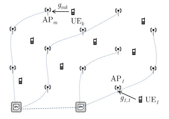
(a)

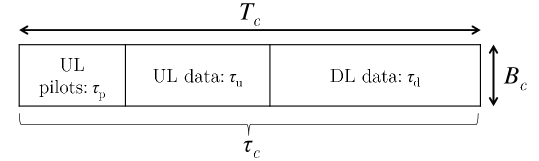
(b)

Figure 1: (a) A CF mMIMO system, where $M$ distributed APs jointly serve $K$ UEs ($K\ll M$). (b) A coherence block with UL pilot training, and UL and DL data transmission phases.

We consider a typical CF mMIMO system, where $K$ single-antenna UEs are jointly served by $M$ geographically distributed APs each equipped with $L$ antennas ($K\ll M$), as shown in Figure 1(a). The APs are connected to one or multiple CPUs by unlimited and error-free fronthaul channels. The CPUs are connected through very fast optical fibers and share the information, and every time one arbitrary CPU is responsible for the pilot assignment. So, our approach is fully centralized, and the study of distributed pilot assignments is left for future work.

The channel coefficient $\textbf{g}_{mk}\in\mathbb{C}^{L\times 1}$ between the $m$-th AP and the $k$-th UE is given as

$$\textbf{g}_{mk}=\beta_{mk}^{1/2}\textbf{h}_{mk},$$ (1)

where $\{\beta_{mk}\}$ represent the large-scale fading (LSF) coefficients, i.e., pathloss and shadowing, and $\{\textbf{h}_{mk}\}$ indicate the small-scale fading coefficients which are assumed to be independent and identically distributed (i.i.d.) normal random variables $\mathcal{CN}(0,\textbf{I}_{L})$. We adopt the block fading model, shown in Figure 1(b), where time-frequency resources are divided into coherence intervals of $\tau_{c}$ channel uses in which the channel can be approximately considered as static. The duration of the intervals is defined based on propagation environment, UEs mobility, and carrier frequency.

Each interval is further divided into three sub-intervals such that: $\tau_{c}=\tau_{p}+\tau_{u}+\tau_{d}$, where $\tau_{p}$ is used for UL pilot training, and $\tau_{u}$ and $\tau_{d}$ are used for UL and DL data transmission, respectively. We assume that $\textbf{h}_{mk}$ stays constant during a coherence interval and is independent in different coherence intervals. We eliminate the DL pilot training phase by assuming channel reciprocity, i.e., the same channel coefficients for the UL and DL transmissions.

II-A Uplink Pilot Training

We assume that there are only $\tau_{p}$ mutually orthogonal pilot sequences with length $\tau_{p}$ each represented as a column $\boldsymbol{\phi}\in\mathbb{C}^{\tau_{p}\times 1}$ of a matrix $\mathbf{\Phi}$, for which we have $\|\boldsymbol{\phi}_{p_{k}}^{H}\boldsymbol{\phi}_{p_{k^{\prime}}}\|=1$ if $p_{k}=p_{k^{\prime}}$, and $\|\boldsymbol{\phi}_{p_{k}}^{H}\boldsymbol{\phi}_{p_{k^{\prime}}}\|=0$, otherwise, and $p_{k}\in\{1,\ldots,\tau_{p}\}$ indicates the index of the pilot assigned to the $k$th UE.

In the UL pilot training phase, all UEs simultaneously transmit their pilots. The $m$-th AP receives

$${\textbf{Y}}_{m}^{\mathrm{p}}=\sqrt{\tau_{p}\rho^{\mathrm{p}}}\sum_{k=1}^{K}\textbf{g}_{mk}\boldsymbol{\boldsymbol{\phi}}_{p_{k}}^{H}+\textbf{W}_{m}^{\mathrm{p}},$$ (2)

where $\rho^{\mathrm{p}}$ is the normalized Signal-to-Noise Ratio (SNR) of a pilot sequence with respect to the noise power, and $\textbf{W}_{m}^{\mathrm{p}}$ is the $L\times\tau_{c}$ additive noise matrix with elements following i.i.d. $\sim\mathcal{CN}(0,1)$ random variables.

As shown in [2, 33], the effective channel coefficients between UE $k$ and AP $m$ can be estimated employing the Minimum Mean Square Error (MMSE) estimator after projecting $\textbf{Y}_{m}^{\mathrm{p}}$ onto $\boldsymbol{\phi}_{k}^{H}$ as

$$\hat{\textbf{g}}_{mk}\!=\mathbb{E}\left\{\textbf{g}_{mk}\check{\textbf{y}}^{\mathrm{p}H}_{mk}\right\}\!\Big{(}\mathbb{E}\left\{\check{\textbf{y}}_{mk}^{\mathrm{p}}\check{\textbf{y}}^{\mathrm{p}H}_{mk}\right\}\Big{)}^{-1}\check{\textbf{y}}_{mk}^{\mathrm{p}}=c_{mk}\check{\textbf{y}}_{mk}^{\mathrm{p}},$$ (3)

where $\check{\textbf{y}}_{mk}^{\mathrm{p}}\triangleq\textbf{Y}^{\mathrm{p}}_{m}\boldsymbol{\phi}_{p_{k}}$, and

$$c_{mk}\triangleq\frac{\sqrt{\tau_{p}\rho^{\mathrm{p}}}\beta_{mk}}{\tau_{p}\rho^{\mathrm{p}}\sum_{k^{\prime}=1}^{K}\beta_{mk^{\prime}}\left|\boldsymbol{\phi}_{p_{k}}^{H}\boldsymbol{\phi}_{p_{k^{\prime}}}\right|^{2}+1}.$$ (4)

The $l$-th component’s mean-square of the estimated channel vector $\hat{\textbf{g}}_{mk}$ can be calculated as

$$\gamma_{mk}\triangleq\mathbb{E}\left\{\left|\left[\hat{\textbf{g}}_{mk}\right]_{l}\right|^{2}\right\}=\sqrt{\tau_{p}\rho^{\mathrm{p}}}\beta_{mk}c_{mk}.$$ (5)

II-B Uplink Data Transmission

In CF mMIMO, all APs and UEs share the same time-frequency resources for data transmission. In the UL, all UEs simultaneously transmit their data to the APs. The AP $m$ receives

$${\textbf{y}}_{m}^{\mathrm{u}}=\sqrt{\rho^{\mathrm{u}}}\sum_{k=1}^{K}\textbf{g}_{mk}\sqrt{\eta_{k}}q_{k}+\textbf{w}_{m}^{\mathrm{u}},$$ (6)

where $q_{k}$ is the signal transmitted by UE $k$ with power $\mathbb{E}\left\{\left|q_{k}\right|^{2}\right\}=1$, $\eta_{k}\in\left[0,1\right]$ shows the power control coefficient, $\rho^{\mathrm{u}}$ indicates the normalized UL SNR and $w_{m}^{\mathrm{u}}\sim\mathcal{CN}(0,1)$ is the additive noise at the receiver.

The Maximal Ratio (MR) combining scheme can be applied to decode the desired signal for a certain UE $k$. AP $m$ sends $\hat{\textbf{g}}^{*}_{mk}\textbf{y}^{\mathrm{u}}_{m}$ to the CPU for data detection. The CPU combines all the received signals for UE $k$ as

$$r^{\mathrm{u}}_{k}=\sum_{m=1}^{M}\sum_{l=1}^{L}\left[\hat{\textbf{g}}_{mk}\right]^{*}_{l}\left[\textbf{y}^{\mathrm{u}}_{m}\right]_{l}.$$ (7)

Following the same procedure as in [2], the signal then can be decomposed at the CPU as

$$r_{k}^{\mathrm{u}}= \underbrace{\sqrt{\rho^{\mathrm{u}}\eta_{k}}q_{k}\mathbb{E}\left\{\sum_{m=1}^{M}\sum_{l=1}^{L}\left[\hat{\textbf{g}}_{mk}\right]^{*}_{l}\left[\textbf{g}_{mk}\right]_{l}\right\}}_{\texttt{DS}_{k}}$$ (8)

$$+\underbrace{\sqrt{\rho^{\mathrm{u}}\eta_{k}}q_{k}\left(\sum_{m=1}^{M}\sum_{l=1}^{L}\left[\hat{\textbf{g}}_{mk}\right]^{*}_{l}\left[\textbf{g}_{mk}\right]_{l}-\mathbb{E}\left\{\sum_{m=1}^{M}\sum_{l=1}^{L}\left[\hat{\textbf{g}}_{mk}\right]^{*}_{l}\left[\textbf{g}_{mk}\right]_{l}\right\}\right)}_{\texttt{BU}_{k}}$$

$$+\underbrace{\sqrt{\rho^{\mathrm{u}}}\sum_{m=1}^{M}\sum_{k^{\prime}\neq k}^{K}\sum_{l=1}^{L}\sqrt{\eta_{k^{\prime}}}\left[\hat{\textbf{g}}_{mk}\right]^{*}_{l}\left[\textbf{g}_{mk^{\prime}}\right]_{l}q_{k^{\prime}}}_{\texttt{CPI}_{k}}+\sum_{m=1}^{M}\sum_{l=1}^{L}\left[\hat{\textbf{g}}_{mk}\right]^{*}_{l}\left[\textbf{w}_{m}^{\mathrm{u}}\right]_{l},$$

where $\texttt{DS}_{k}$, $\texttt{BU}_{k}$ and $\texttt{CPI}_{k}$ denoted the desired signal (DS), beamforming uncertainty (BU) and co-pilot interference (CPI), respectively.

The UL achievable rate for UE $k$ can be calculated as

$$\operatorname{R}_{k}^{\mathrm{u}}=\log_{2}\left(1+\frac{L^{2}\rho^{\mathrm{u}}\eta_{k}\left(\sum_{m=1}^{M}\gamma_{mk}\right)^{2}}{L^{2}\rho^{\mathrm{u}}\sum_{k^{\prime}\neq k}^{K}\eta_{k^{\prime}}\left(\sum_{m=1}^{M}\gamma_{mk}\frac{\beta_{mk^{\prime}}}{\beta_{mk}}\right)^{2}\left|\boldsymbol{\phi}_{p_{k}}^{H}\boldsymbol{\phi}_{p_{k^{\prime}}}\right|+L\rho^{\mathrm{u}}\sum_{k^{\prime}=1}^{K}\eta_{k^{\prime}}\sum_{m=1}^{M}\gamma_{mk}\beta_{mk^{\prime}}+L\sum_{m=1}^{M}\gamma_{mk}}\right).$$ (9)

II-C Downlink Data Transmission

In DL, APs receive encoded data from their CPUs and carry out the transmit precoding, based on the local CSI. The $k$th UE receives signal

$$r_{k}^{\mathrm{d}}=\sqrt{\rho^{\mathrm{d}}}\sum_{m=1}^{M}\sum_{k^{\prime}=1}^{K}\eta_{mk^{\prime}}^{1/2}\textbf{g}^{T}_{mk}\hat{\textbf{g}}^{*}_{mk^{\prime}}q_{k^{\prime}}+w_{k}^{\mathrm{d}},$$ (10)

where $\rho^{\mathrm{d}}$ is the normalized UL SNR, and $w_{k}^{\mathrm{d}}\sim\mathcal{CN}(0,1)$ is the additive noise at the $k$th UE. Then $q_{k}$ will be detected from $r_{k}^{\mathrm{d}}$.

Employing a similar methodology as in the UL, the achievable DL rate for the $k$th UE can be derived from

$$\operatorname{R}_{k}^{\mathrm{d}}=\log_{2}\left(1+\frac{L^{2}\rho^{\mathrm{d}}\left(\sum_{m=1}^{M}\eta_{mk}^{1/2}\gamma_{mk}\right)^{2}}{\rho^{\mathrm{d}}\sum_{k^{\prime}\neq k}^{K}\left(\sum_{m=1}^{M}\eta_{mk^{\prime}}^{1/2}\gamma_{mk^{\prime}}\frac{\beta_{mk}}{\beta_{mk^{\prime}}}\right)^{2}\left|\boldsymbol{\phi}_{k^{\prime}}^{H}\boldsymbol{\phi}_{k}\right|^{2}+L\rho^{\mathrm{d}}\sum_{k^{\prime}=1}^{K}\sum_{m=1}^{M}\eta_{mk^{\prime}}\gamma_{mk^{\prime}}\beta_{mk}+1}\right).$$ (11)

III Pilot Assignment in CF mMIMO

III-A Problem formulation

The goal of the UL pilot training phase is to increase the number of effectively estimated channels or to improve the quality of the UL channel estimation, which can be interpreted as a UL rate maximization problem. So, an efficient pilot reuse scheme should assign pilots to UEs so that the sum of the UL rates is maximized. Mathematically the pilot reuse problem in CF mMIMO can be formulated as

—s—[1] p ∑_k=1^K R_k^u p=[p_1,…,p_K]^T ϕ_p_k=col_p_k(Φ) p_k∈{1,…,τ_p}, where the p is the pilot assignment vector and $\mathrm{col}_{i}(\boldsymbol{\Phi})$ indicates the $i$th column of matrix $\boldsymbol{\Phi}$.

The co-pilot interference originated from reusing the same pilot for similar UEs, i.e., geographical closeness, common serving APs, and similar channel coefficients. So, an intelligent pilot assignment scheme should consider the similarity among the UEs and reuse the same pilot $\boldsymbol{\phi}$ in UEs that have higher dissimilarities, i.e., geographically far apart or with fewer common serving APs. We hence formulate the pilot assignment in CF mMIMO as a diverse clustering problem, where we form $\tau_{p}$ (number of available orthogonal pilots) clusters in such a way that UEs belonging to the same cluster have a high “dissimilarity” or “diversity”. In the following subsection, we formulate and discuss the problem.

III-B Diverse Clustering Problem

The DCP consists of the assigning of a set of $K$ elements, i.e., UEs, into $\tau_{p}$ mutually disjoint subsets or clusters, i.e., pilots, while the diversity among the elements in each subset, i.e., intra-cluster diversity, and inter-cluster similarity is maximized. The inter-cluster diversity is calculated as the sum of the individual distances between each pair of elements in clusters, where the concept of distance depends on the specific application context. The objective is to maximize the overall diversity, i.e., the sum of the diversity of all subsets. From the graph theory perspective, DCP can be considered as partitioning the vertices of a complete weighted undirected graph into $\tau_{p}$ subgraphs in such a way that the total weight of the subgraphs is maximized while applying optional constraints on the number of nodes in each subgraph.

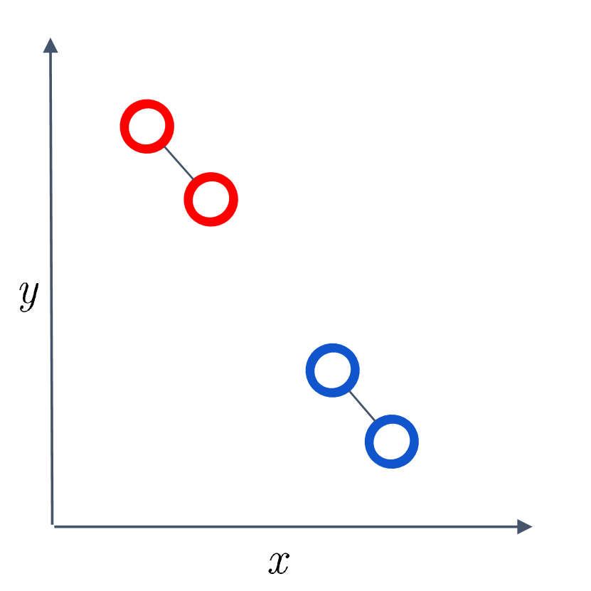
(a)

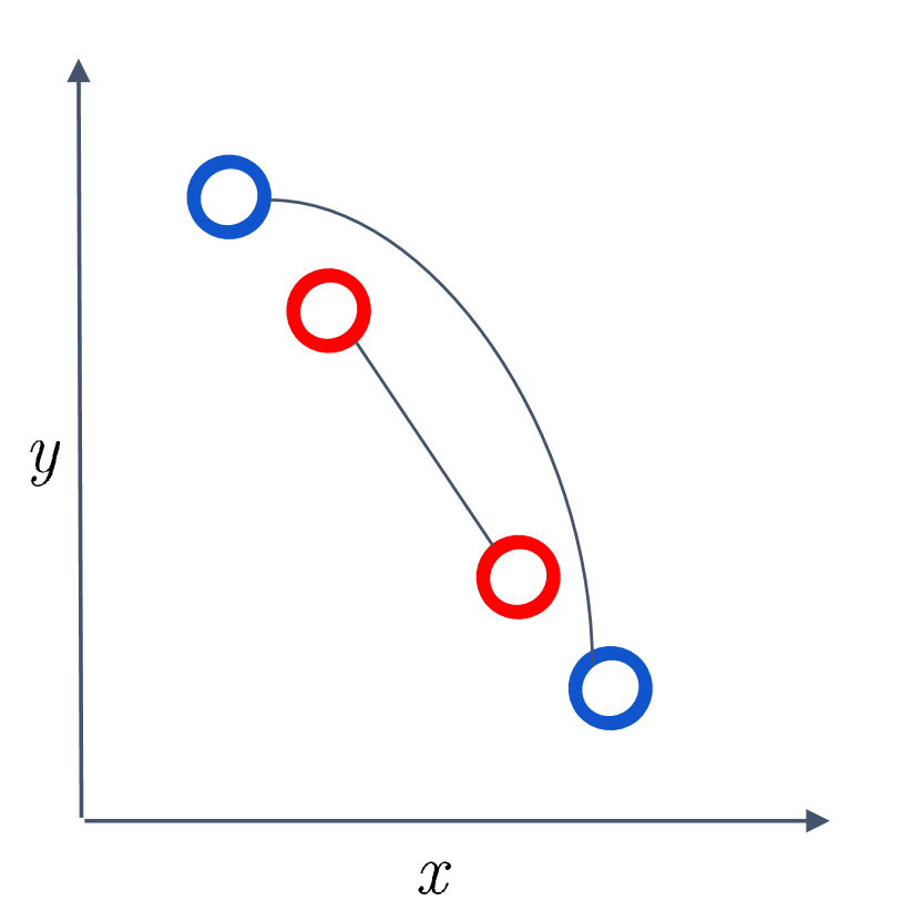
(b)

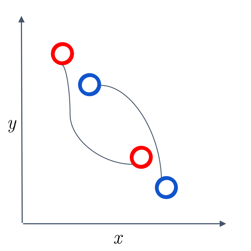
(c)

Figure 2: Illustrated example and comparison of the conventional clustering (a), and feasible (b) and optimal (c) solutions for diverse clustering, with four data points and two clusters.

An illustration of DCP and of the conventional clustering problem is presented in Figure 2 for a small configuration with four data points and two clusters. Figure 2(a) shows a conventional clustering problem, where clusters are formed in such a way to minimize inter-cluster similarity (intra-cluster diversity).

In contrast, Figure 2b-c show two DCPs, where data points with higher dissimilarities are joining the same cluster. Figure 2(b) represents a feasible solution for DCP, in which the diversity score of one cluster (blue data points) is relatively higher than the other, while in the optimal solution, all clusters should have relatively similar diversity score, as it is the case in Figure 2(c).

In general DCP can be considered as a capacitated clustering [34, 35] or maximally diverse grouping problem [36, 37] and then formulated as a quadratic integer program as —s—[1] X ∑_p=1^τ_p ∑_k=1^K-1∑_k′=k+1^K x_k,px_k’,pd_k,k’ ∑_p=1^τ_px_k,p=1,  k=1,…,K L_k ≤∑_k=1^K x_k,p≤U_k, p=1,…,τ_p x_k,p∈{0,1},   k=1,…,K, p=1,…,τ_p, where $\textbf{X}\in\{0,1\}^{K\times\tau_{p}}$ is a binary association matrix, and $x_{k,p}=1$ if element (UE) $k$ belongs to cluster (pilot) $p$, and $x_{k,p}=0$ otherwise. $d_{k,k^{\prime}}$ is the diversity measure between $k$ and $k^{\prime}$ elements, and $L_{b}$ and $U_{b}$ show the minimum and maximum size of each set, respectively. The constraint (2) guarantees that each element is assigned to only one cluster, and (2) forces the size of the clusters to be in the specified range. The diversity measure can be a predefined distance function, i.e., Euclidean distance and cosine similarity, or can be defined as a parameterized kernel and then learned by, e.g., neural networks.

This formulation favors forming fewer large-size clusters against many small-size clusters. Considering the full interference among the nodes in each cluster (orthogonal pilot), in the pilot reuse problem, fewer large-size clusters increase the co-pilot interference among the co-cluster UEs. So we multiply a regularization term by the objective of the optimization problem to penalize the large-size clusters by dividing their score by the size of clusters. This will avoid wasteful growth of the size of some clusters. Adding a new node to a $N$-size cluster is interpreted as interference with all $N$ nodes and penalized. Hence, the new formulation will be

—s—[1] X ∑_p=1^τ_p 1—Cp—∑_k=1^K-1∑_k′=k+1^K x_k,px_k’,pd_k,k’ (2) - (2) where $\mathcal{C}_{p}$ is the cluster set $p$, and $|\cdot|$ shows the size of a set.

DCP is a combinatorial optimization problem and is proved to be NP-hard [38]. Typically finding the exact solution for these problems is not computationally possible, at least when $K$ is large.

DCP has already been investigated in the literature under different names, such as maximally diverse grouping problem  [36] and anticlustering [39, 40]. Several algorithms have already been proposed to solve DCP, including tabu search with strategic oscillation [41], genetic algorithm [42, 43], artificial bee colony [44], variable neighborhood search [37]. In this paper, we propose an iterative maxima search method, adopted from [45], for pilot reuse in CF mMIMO based on DCP problem.

IV Iterative Maxima Search for Pilot Reuse

The proposed approach employs an iterative maxima search procedure that integrates a local neighborhood search procedure with a weak perturbation operator to improve the intensity or quality of solutions and a robust perturbation operator to improve the diversity of the solutions by moving the search to a distant region to avoid local optimum solutions. Before going to the details of the proposed scheme, some concepts need to be defined.

Definition of neighborhoods

We define two different types of neighborhood: OneMove ($N_{1}$) neighborhood and SwapMove ($N_{2}$) neighborhood. Given the pilot assignment vector p, $N_{1}$ returns all possible solutions obtained by changing the assigned pilot of a single UE (OneMove) in such a way that the pilot reuse capacity constraints are satisfied, while $N_{2}$ returns the possible solutions obtained by exchanging the pilots of a pair of UEs (SwapMove).

M matrix

To improve the computational efficiency of the local search procedure, we employ a $K\times\tau_{p}$ matrix M, where $m_{k,p}\in\textbf{M}$ shows the sum of diversity between UE $k$ and all UEs with pilot index $p$, and having the pilot assignment vector p, calculates as $m_{k,p}=\sum_{\begin{subarray}{c}k,k^{\prime}=1,\\ p_{k^{\prime}}=p\end{subarray}}^{K}d_{k,k^{\prime}}$. Calculation of this matrix can be done in order of $\mathcal{O}(K^{2})$.

Definition of a solution

The tuple $<\textbf{p},\mathbf{c},\mathbf{s}>$ refers to a solution in search space, where $\mathbf{c}$ is a vector that saves the diversity index of each cluster, and $\mathbf{s}$ is a vector that stores the size of each cluster for a given solution. Basically, for each solution in the search space, we save and update the tuple where the two last elements are used to speed up the search procedure, as we will discuss later.

The overall procedure is presented in Algorithm 1. The algorithm starts by generating $I_{s}$ random initial feasible solutions (Algorithm 2), followed by a local neighborhood search procedure (Algorithm 3). The best solution among the initial solutions is then saved for later use. It then repeats a maxima search procedure (lines 9-20) followed by a robust perturbation procedure until a certain time budget is exceeded. This iterative maxima search procedure is composed of a weak perturbation procedure (Algorithm 4) followed by a local search procedure (Algorithm 3), which will be discussed in the following subsections. In each iteration, after employing the weak perturbation and local search procedures, the quality or fitness of the current solution p ($f(\textbf{p})$) is compared and used to replace the incumbent solution $\textbf{p}^{*}$ in case of improvement (lines 14-19). The fitness of a solution is calculated as:

$$f(\textbf{p})=\sum_{p=1}^{\tau_{p}}\frac{1}{|\mathcal{C}_{p}|}\sum_{\begin{subarray}{c}p_{k}=p_{k^{\prime}},\\ k<k^{\prime}\end{subarray}}d_{kk^{\prime}},$$ (12)

where, $d_{kk^{\prime}}$ represents the diversity among $k$ and $k^{\prime}$ UEs. This fitness function basically is a weighted average of the diversity score of different clusters, where the weight is the inverse of the cluster size.

Algorithm 1 Iterative Maxima Search for Pilot Reuse

Input: $I_{s}$, $t_{max}$, $\alpha$  
Output: Pilot assignment vector $\textbf{p}^{*}$

1:Initialize empty set $\mathcal{P}_{0}$

2:for $i=1\ \textbf{to}\ I_{s}$ do

3:     Generate initial solution $\textbf{p}^{0}$ employing Algorithm 2.

4:     Update $\textbf{p}^{0}$ employing the local search in Algorithm 3.

5:     Add $\textbf{p}^{0}$ to $\mathcal{P}_{0}$.

6:end for

7:Get the best solution from $\mathcal{P}_{0}$ and save it in p

8:$\textbf{p}^{*}\leftarrow\textbf{p}$

9:while $Time()\leq t_{max}$ do

10:     Set $ctr\leftarrow 0$

11:     while $ctr<\alpha$ do

12:         Apply weak perturbation operator in Algorithm 4 on p.

13:         Update p employing local search Algorithm 3.

14:         if $f(\textbf{p})>f(\textbf{p}^{*})$ then

15:              $\textbf{p}^{*}\leftarrow\textbf{p}$

16:              Reset $ctr\leftarrow 0$

17:         else

18:              Increase $ctr\leftarrow ctr+1$

19:         end if

20:     end while

21:     Update p employing the robust perturbation in Algorithm 5.

22:end while

23:Return $\textbf{p}^{*}$

IV-A Initial Feasible Solution

The Initial feasible solution procedure is presented in Algorithm 2. The procedure starts by randomly assigning each pilot to $L_{b}$ UEs and then for the remaining UEs assigns a random pilot $p$ while being sure that the number of UEs with pilot $p$, $|\mathcal{C}_{p}|$, is less than an upper bound $U_{b}$. The complexity of this algorithm is $\mathcal{O}(K+\tau_{p})$.

Algorithm 2 Initial Feasible Solution

Input: Set of Pilots $\mathcal{P}$, Set of UEs $\mathcal{K}$, $L_{b}$, $U_{b}$ 
Output: Initial Pilot Assignment Vector p

1:for $p\in\mathcal{P}$ do

2:     Randomly select $L_{b}$ UEs from $\mathcal{K}$ and name it $\mathcal{K^{\prime}}$ 

3:     Assign pilot $p$ to UEs in $\mathcal{K^{\prime}}$ and update $\mathcal{K}=\mathcal{K}\setminus\mathcal{K^{\prime}}$ 

4:end for

5:while $\mathcal{K}\neq\emptyset$ do

6:     Get $k\in\mathcal{K}$ and randomly select pilot $p\in\mathcal{P}$ 

7:     if $|\mathcal{C}|_{p}<U_{b}$ then

8:         Assign pilot $p$ to $k$ and update $\mathcal{K}=\mathcal{K}\setminus\{k\}$ 

9:     end if

10:end while

11:Return assignment vector p.

IV-B Local Neighborhood Search

The local neighborhood search procedure is presented in Algorithm 3. Given the current assignment p, the procedure probes $N_{1}(\textbf{p})$ (lines 3-11) and $N_{2}(\textbf{p})$ (lines 12-19) neighborhoods and iteratively updates the incumbent solution with the better neighbor solution. The procedure repeats until the incumbent solution finds the local optimum and can not be further improved. Given a solution $<\textbf{p},\mathbf{c},\mathbf{s}>$, the fitness of a neighbor solution can be easily computed using the defined above matrix M. For $N_{1}$ neighbors, changing the pilot index of UE $k$ from $i$ to $j$ does not change the diversity values of the UEs, except those with pilot index $i$ and $j$. Here the value of a OneMove can be determined by

$$\Delta f=\frac{c_{j}+m_{kj}}{s_{j}+1}-\frac{c_{j}}{s_{j}}+\frac{c_{i}-m_{ki}}{s_{i}-1}-\frac{c_{i}}{s_{i}},$$ (13)

where $m_{k,i}$ and $m_{k,j}$ are the entries of matrix M and $c$, and $s$ are the elements of vectors c and s, respectively.

Also for $N_{2}$ neighbors, the value of a SwapMove (exchanging the pilot index of UEs $k$ and $k^{\prime}$) is determined by

$$\Delta f=(m_{k,p_{k^{\prime}}}-m_{k,p_{k})+(m_{k^{\prime},p_{k}}-m_{k^{\prime},p_{k^{\prime}}})-2d_{kk^{\prime}}}.$$ (14)

Algorithm 3 Local Search Procedure

Input: Set of Pilots $\mathcal{P}$, Set of UEs $\mathcal{K}$, p, $L_{b}$, $U_{b}$ 
Output: Local optimum assignment $\textbf{p}^{*}$

1:$\textbf{p}^{*}\leftarrow\textbf{p}$

2:Initialize $\textbf{M}\in\mathbb{R}^{K\times\tau_{p}}$ 

3:while solution improves do

4:     for $k\in\mathcal{K}\land p\in\mathcal{P}$ do

5:         if $(p^{*}_{k}\neq p)\land(\mathcal{C}_{p^{*}_{k}}>L_{b})\land(\mathcal{C}_{p}<U_{b})$ then

6:              Calculate $\Delta f$ by (13)

7:              if $\Delta>0$ then

8:                  Set $p^{*}_{k}\leftarrow p$ and update M

9:              end if

10:         end if

11:     end for

12:     for $k,k^{\prime}\in\mathcal{K}\land k^{\prime}>k$ do

13:         if $p^{*}_{k}\neq p^{*}_{k^{\prime}}$ then

14:              Calculate $\Delta f$ by (14)

15:              if $\Delta f>0$ then

16:                  Swap the pilots of $k$ and $k^{\prime}$ and update M

17:              end if

18:         end if

19:     end for

20:end while

21:Return $\textbf{p}^{*}$

IV-C Weak and robust perturbation

The weak and robust perturbation procedures are presented in Algorithm 4 and Algorithm 5, respectively. The weak perturbation operator aims to jump out of the current local optimum within the iterative search procedure by applying some assignment deterioration. The strength of the weak perturbation is controlled by $\eta_{w}$, representing the number of random neighbor solutions to be checked by this operator. For each perturbation step, the best solution among $\eta_{w2}$ randomly selected neighbors is compared, and the incumbent solution is replaced in case of improvement (lines 3-7). This incumbent solution is used for the next iteration of perturbation. The large values of $\eta_{w2}$ cause less deterioration of the current sample and can be set to $K$ to adjust the problem size.

Algorithm 4 Weak Perturbation

Input: Pilot assignment vector p, $\eta_{w}$, $\eta_{w}2$
Output: Perturbed assignment p

1:for $i=1\ \textbf{to}\ \eta_{w}$ do

2:      Randomly select a neighbor solution $\textbf{p}^{\prime}\in N_{1}(\textbf{p})\cup N_{2}(\textbf{p})$

3:     for $j=1\ \textbf{to}\ \eta_{w2}$ do

4:          Randomly select a neighbor solution $\textbf{p}^{\prime\prime}\in N_{1}(\textbf{p})\cup N_{2}(\textbf{p})$

5:         if $f(\textbf{p}^{\prime\prime})>f(\textbf{p'})$ then

6:              $\textbf{p}^{\prime}\leftarrow\textbf{p}^{\prime\prime}$

7:         end if

8:     end for

9:     $\textbf{p}\leftarrow\textbf{p}^{\prime}$

10:end for

11:Return assignment vector p.

The weak perturbation helps the search procedure discover the neighborhood of the current area better, while it is still possible that the search is trapped in a deep local optimum that weak perturbation can not jump out of. The robust perturbation procedure consequently performs $\eta_{s}$ moves regardless of their values. $\eta_{s}$ controls the strength of the robust perturbation and is empirically set to $\eta_{s}=\theta\times\frac{K}{\tau_{p}}$, from [45], where $\theta$ is chosen from $\{1,1.5\}$.

Algorithm 5 Robust Perturbation

Input: Pilot assignment vector p, $\eta_{s}$
Output: Perturbed assignment p

1:for $i=1\ \textbf{to}\ \eta_{w}$ do

2:      Randomly select a neighbor solutions $\textbf{p}^{\prime}\in N_{1}(\textbf{p})\cup N_{2}(\textbf{p})$

3:     $\textbf{p}\leftarrow\textbf{p}^{\prime}$

4:end for

5:Return assignment vector p.

V Numerical results

V-A Simulation setup

Let us consider $M$ APs with $L$ antennas and $K$ single antenna UEs that are independently and uniformly distributed in a $1\times 1$ km² square area. The wraparound technique is adopted to mitigate the network edge and boundary effects and to model the network as if operating over an unlimited area. The large-scale fading coefficient $\beta_{mk}$ in (1) is calculated by $\beta_{mk}=\mathrm{PL}_{mk}\cdot 10^{\sigma_{sh}z_{mk}}/10$, where $10^{\sigma_{sh}z_{mk}}/10$ represents the shadow fading with standard deviation $\sigma_{sh}$ and $z_{mk}\sim\mathcal{N}(0,1)$ and $\mathrm{PL}_{mk}$ represents the pathloss from UE $k$ to AP $m$. In this paper, we use the three-slope path loss model presented in [2] as

$$\mathrm{PL}_{mk}=\left\{\begin{array}[]{l}-L-15\log_{10}\left(d_{1}\right)-20\log_{10}\left(d_{0}\right),\text{ if }d_{mk}\leq d_{0}\\ -L-15\log_{10}\left(d_{1}\right)-20\log_{10}\left(d_{mk}\right)\\ \text{ if }d_{0}<d_{mk}\leq d_{1}\\ -L-35\log_{10}\left(d_{mk}\right),\text{ if }d_{mk}>d_{1}\par\end{array}\right.$$ (15)

where $d_{mk}$ indicates the distance between AP $m$ and UE $k$, $d_{0}$ and $d_{1}$ are the distance thresholds, and $L$ is given by

$$L\triangleq \quad 46.3+33.9\log_{10}(f)-13.82\log_{10}\left(h_{\mathrm{AP}}\right)$$ (16)

$$\quad-\left(1.1\log_{10}(f)-0.7\right)h_{\mathrm{u}}+\left(1.56\log_{10}(f)-0.8\right),$$

where $f$ (MHz) is the carrier frequency, and $h_{\mathrm{u}}$ (m) and $h_{\mathrm{AP}}$ (m) indicate the UE and AP height respectively.

Noise power is calculated by $P_{n}=Bk_{B}T_{0}W$, where $B$ is the bandwidth, $k_{B}$ denotes the Boltzmann constant, $T_{0}$ is the noise temperature and $W$ represents the noise figure. The transmission powers of the uplink pilot and the uplink data and downlink data are set to $\rho^{\mathrm{p}}=100$ (mW), $\rho^{\mathrm{u}}=100$ (mW), and $\rho^{\mathrm{d}}=200$ (mW), respectively. The channel estimation overhead has been taken into account in defining the per-user uplink throughput as $T_{k}^{\mathrm{u}}=B\frac{1-\tau_{p}/\tau_{c}}{2}\log_{2}(1+\operatorname{SINR}^{\mathrm{u}}_{k})$, where $\tau_{c}=200$ samples. The $1/2$ in the above equation is due to the co-existence of the uplink and downlink traffic. We also employed max-min power control [2] to further improve the sum throughput.

In this paper we consider the Euclidean distance for the diversity measure as $d_{k,k^{\prime}}=\sqrt{\sum_{i=1}^{|F|}(U_{k}[i]-U_{k^{\prime}}[i])^{2}}$, where $F$ is the feature set (e.g., geographical coordinates) of the UEs. The definition and analysis of more sophisticated repulsive functions are left for future work.

TABLE I: Simulation setup.

Parameter	Value	Definition
$B$	20 MHz	Bandwidth
$h_{\mathrm{u}}$	1.65 m	UE height
$h_{\mathrm{AP}}$	15 m	AP height
$d_{0}$, $d_{1}$	10 m, 50 m	Path loss distance thresholds
$k_{B}$	$1.381\times 10^{-23}$ (Joule per Kelvin)	Boltzmann constant
$T_{0}$	290 (Kelvin)	Noise temperature
$W$	9	Noise figure
$\rho^{\mathrm{p}}$	100 mW	Pilot transmission power
$\rho^{\mathrm{u}}$	100 mW	Uplink transmission power
$\rho^{\mathrm{d}}$	200 mW	Downlink transmission power

V-B Result and discussion

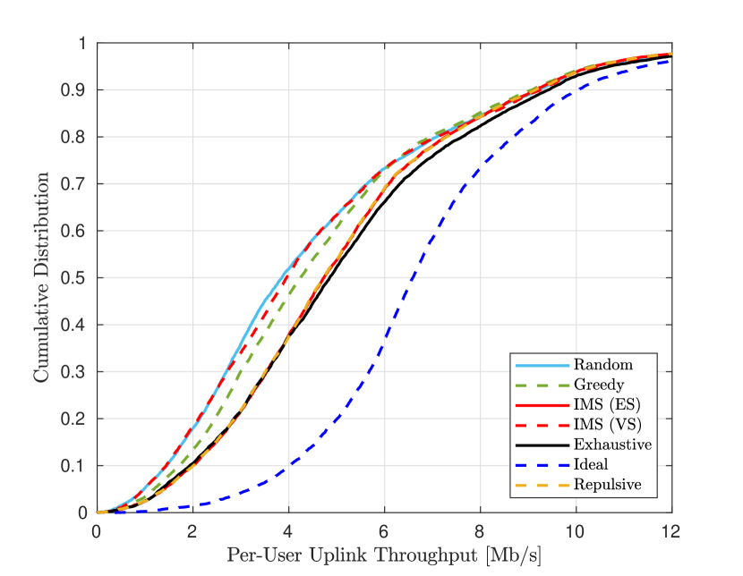
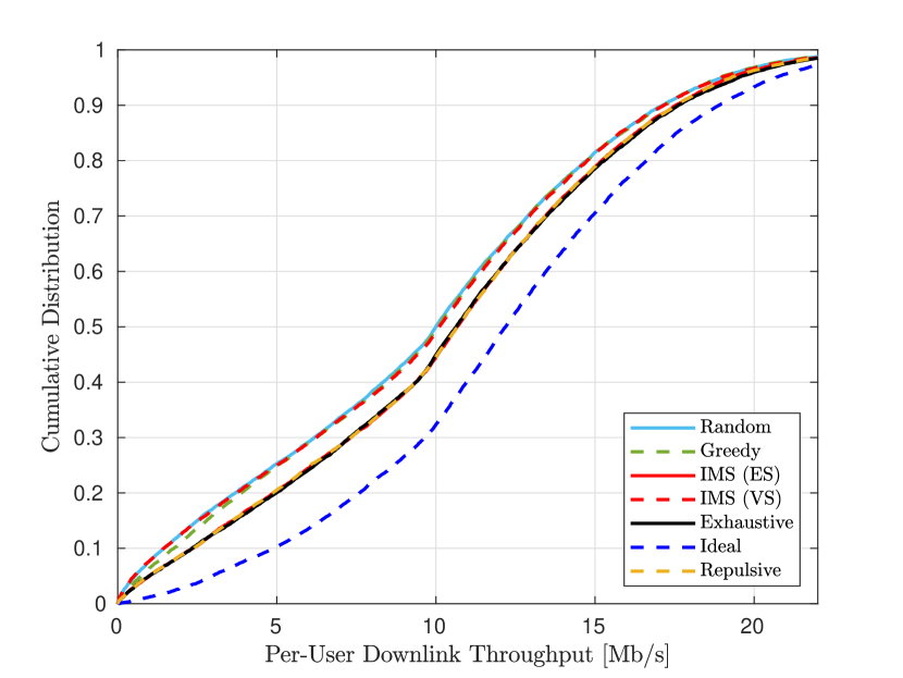
Figure 3: Cumulative distribution of the per-user uplink and downlink throughput for different pilot assignment strategies for a small-scale scenario, $M=50$, $K=12$, $L=1$, and $\tau_{p}=3$.

This section compares the result of the proposed Iterative Maxima Search (IMS) scheme against different pilot assignment strategies. In particular, the random and greedy pilot assignments from [2], the repulsive clustering [32] and the Ideal solution are chosen for evaluation. The ideal solution represents the unreachable upper bound, where there is no pilot contamination (i.e., $\mathrm{CPI}_{k}=0$ in (8)) and the channels can be perfectly estimated only having one single pilot. Two different variants of our algorithm are considered: equal size (ES) clusters and variable size (VS) clusters. The former keeps $L_{b}=U_{b}$, while the latter does not have such constraint, and the algorithm can form clusters of any size.

Figure 3 shows the per-user throughput Cumulative Distribution Function (CDF) of different pilot reuse policies for the small-scale scenario for the sake of comparison with the exhaustive search. (As the complexity of exhaustive search grows exponentially with the number of UEs, calculating its performance for large $M$ is not possible.) The figure shows that the proposed method outperforms other approaches both in UL and DL and works almost as well as the optimal pilot reuse obtained by exhaustive search, but with far less complexity.

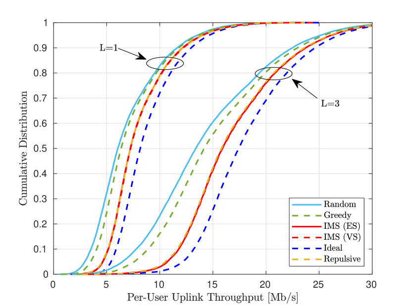
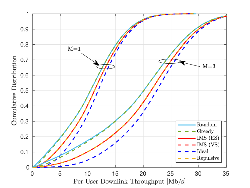
Figure 4: Cumulative distribution of the per-user uplink and downlink throughput for different pilot assignment strategies, $K=40$, $\tau_{p}=10$, and $M=200$.

The cumulative distribution of the per-user uplink and downlink throughput of different pilot assignment strategies for different numbers of antennas $L$ is shown in Figure 4. The superiority of the proposed scheme against other approaches is evident from the figure. It can also be seen from the figure that increasing the number of antennas per AP will increase the rate in all schemes while the gap between the proposed scheme and other algorithms also increases, which is reasonable as our scheme generates less co-pilot interference by properly utilizing the available resources.

TABLE II: 95th percentile of per-user uplink and downlink throughput for different values of $L$, when $K=40$, $\tau_{p}=10$, and $M=200$.

Approach	UL		DL
	L=1	L=3	L=1	L=3
Random	2.93	6.49	1.43	3.31
Greedy	3.49	7.59	1.68	4.16
Repulsive	4.59	10.52	2.69	6.80
IMS (ES)	4.62	10.71	2.73	6.90
IMS (VS)	4.63	10.68	2.72	6.88
Ideal	5.40	12.20	4.18	10.09

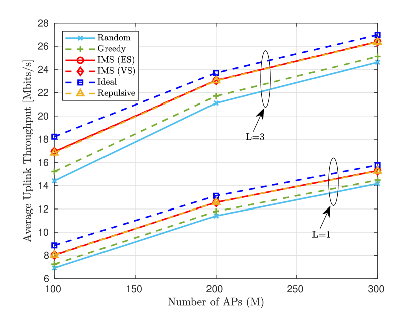
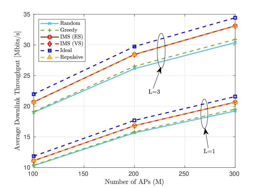
Figure 5: Average uplink and downlink throughput for different pilot assignment strategies, $K=40$, $\tau_{p}=10$.

Table II shows the 95th percentile of the per-user throughput extracted from Figure 4, where it can be seen that increasing the number of APs’ antennas from $L=1$ to $L=3$ increases the 95th percentile by 2.3x for uplink and 2.5x for downlink. Compared to other schemes, our approach performs slightly better than repulsive clustering, but it improves the 95th percentile rate by 1.13 Mbps ($\approx 32\%$) in uplink and 1.05 Mbps ($\approx 62\%$) in downlink over a greedy pilot assignment scheme, when $L=1$. These values for $L=3$ are 3.12 Mbps ($\approx 38\%$) and 2.74 Mbps ($\approx 65\%$).

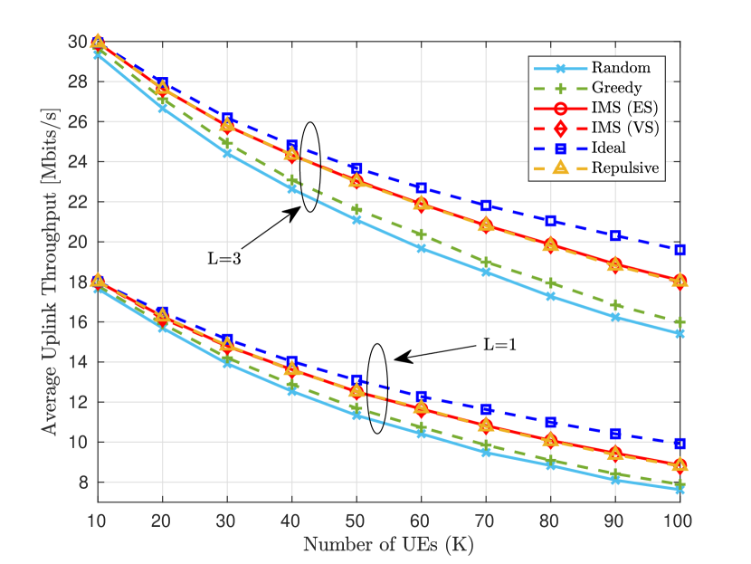
Figure 6: Average uplink throughput for different numbers of UEs, $M=100$ and $\tau_{p}=10$.

Figure 5 compares the average uplink and downlink throughput against different numbers of APs for different pilot reuse schemes. By increasing the number of APs, the average throughput increases in both uplink and downlink. Also, the performance of the multiple-antenna APs is always better than that of single-antenna APs. For example, having 100 APs with three antennas (300 antennas in total) performs better than 300 single-antenna APs. This comes from the fact that increasing $L$ makes the channel more favorable [46] and reduces inter-user interference. It also increases the array gain, which has already been discussed and analyzed in [47].

The average uplink and downlink throughput of different pilot assignment schemes against the number of UEs is illustrated in Figure 6. It can be seen from the figure that increasing the number of UEs in the network, while the number of APs is fixed, will decrease the average throughput. The throughput reduction ratio is different for the pilot assignment policies, and in our approach it is lower than in the random and greedy schemes. This shows the reliability of our approach in large-scale scenarios.

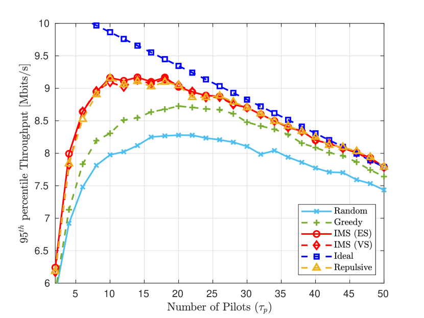
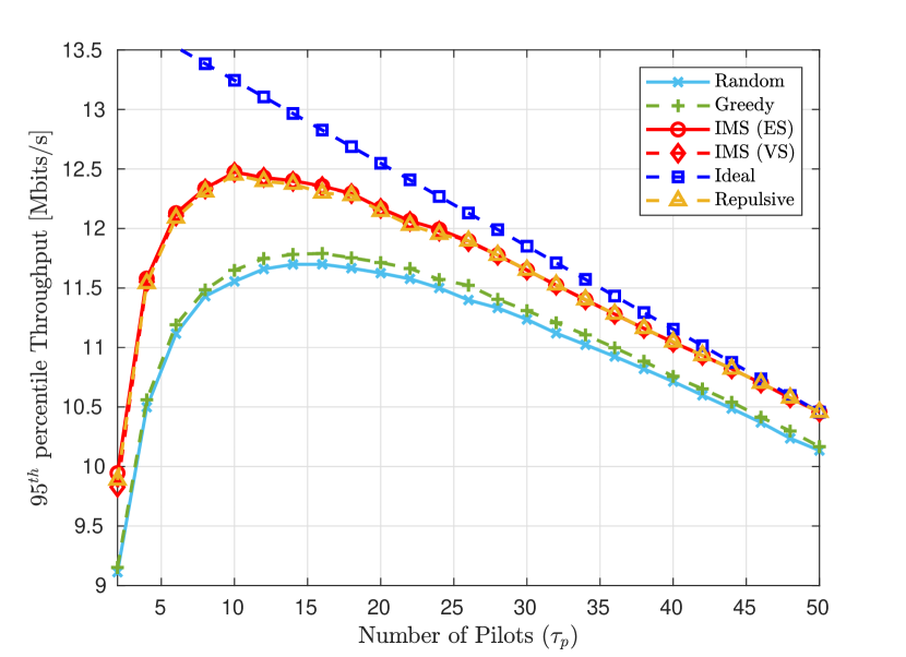
Figure 7: Average the per-user uplink and downlink throughput for different numbers of orthogonal pilots, $M=100$, $L=1$, and $K=50$.

Figure 7 presents the average uplink and downlink throughput with respect to the number of orthogonal pilots ($\tau_{p}$) for different pilot assignment schemes, while the size of the coherence block is fixed. An interesting fact that can be seen in the figures is that increasing the number of pilots increases the performance only up to a certain point, after which the performance starts decreasing. This shows the necessity of finding the optimal number of pilots, which is outside this paper’s scope and is left for future research.

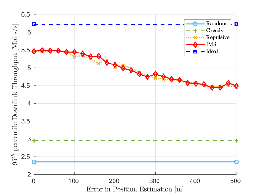
Figure 8: Average uplink and downlink throughput for different values of error in location estimation, $M=120$, $K=50$, $K=10$, and $L=1$.

Figure 8 shows the 95^th percentile rate of the proposed schemes in the presence of errors in the UEs locations estimation. As seen in the figure, the proposed algorithms, until a certain level, are robust against errors, and the system performance is not affected much when the error in the location estimation is less than 100 meters. Even after that, the rate is higher than in random and greedy schemes.

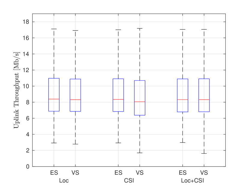
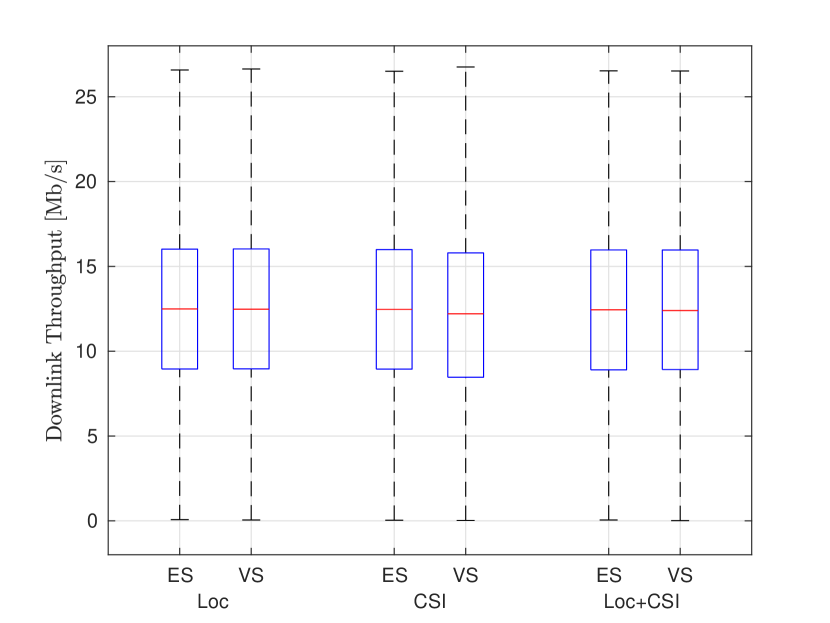
Figure 9: Uplink and downlink throughput when location and/or CSI is used as input feature for clustering.

Figure 9 shows the uplink and downlink throughput for UEs when the CSI (LSF) and/or UE’s locations are considered as input features in our clustering algorithm. The figure shows that both features provide relatively similar results, so each can be used as input when the other feature’s data is unavailable. It can also be seen that combining both features does not provide better solutions, and considering only one feature space is enough.

VI Conclusion

CF mMIMO will be an essential part of future wireless communication systems, given its capability of providing uniform service for the UEs. The performance of these systems can still be further improved before it becomes a functional and operational technology. Pilot contamination is recognized as an undesirable effect that can highly degrade the performance of CF mMIMO when the UEs share the same pilot. In this paper, we formulated pilot assignment in CF mMIMO systems as a DCP problem and proposed an iterative maxima search approach to solve it. Numerical results show the proposed scheme’s effectiveness compared to other approaches from the literature. In future works, we will expand our approach by replacing the Euclidean distance with more sophisticated and parameterized diversity functions, i.e., Deep Neural Networks (DNNs) that consider different networking factors such as AP locations, and the density of UEs and APs. Another extension will consider pilot assignment jointly with pilot power control, which can further improve the channel estimation performance. The scalability of different pilot assignment strategies is another factor that should be considered in future research.

References

- [1] H. Q. Ngo, A. Ashikhmin, H. Yang, E. G. Larsson, and T. L. Marzetta, “Cell-Free Massive MIMO: Uniformly great service for everyone,” in IEEE 16th International Workshop on Signal Processing Advances in Wireless Communications (SPAWC), 2015, pp. 201–205.
- [2] H. Q. Ngo, A. Ashikhmin, H. Yang, E. G. Larsson, and T. L. Marzetta, “Cell-Free Massive MIMO Versus Small Cells,” IEEE Transactions on Wireless Communications, vol. 16, no. 3, pp. 1834–1850, March 2017.
- [3] J. Zhang, S. Chen, Y. Lin, J. Zheng, B. Ai, and L. Hanzo, “Cell-Free Massive MIMO: A New Next-Generation Paradigm,” IEEE Access, vol. 7, pp. 99 878–99 888, August 2019.
- [4] Ö. T. Demir, E. Björnson, L. Sanguinetti et al., “Foundations of User-Centric Cell-Free massive MIMO,” Foundations and Trends® in Signal Processing, vol. 14, no. 3-4, pp. 162–472, 2021.
- [5] G. Interdonato, E. Björnson, H. Quoc Ngo, P. Frenger, and E. G. Larsson, “Ubiquitous Cell-free Massive MIMO Communications,” EURASIP Journal on Wireless Communications and Networking, vol. 2019, no. 1, pp. 1–13, August 2019.
- [6] S. Elhoushy, M. Ibrahim, and W. Hamouda, “Cell-Free Massive MIMO: A Survey,” IEEE Communications Surveys & Tutorials, vol. 24, no. 1, pp. 492–523, First Quarter 2022.
- [7] E. Björnson and L. Sanguinetti, “Scalable Cell-Free Massive MIMO Systems,” IEEE Transactions on Communications, vol. 68, no. 7, pp. 4247–4261, July 2020.
- [8] L. Lu, G. Y. Li, A. L. Swindlehurst, A. Ashikhmin, and R. Zhang, “An Overview of Massive MIMO: Benefits and Challenges,” IEEE Journal of Selected Topics in Signal Processing, vol. 8, no. 5, pp. 742–758, October 2014.
- [9] T. L. Marzetta, “Massive MIMO: An Introduction,” Bell Labs Technical Journal, vol. 20, pp. 11–22, 2015.
- [10] T. L. Marzetta and H. Yang, Fundamentals of massive MIMO. Cambridge University Press, 2016.
- [11] E. G. Larsson, O. Edfors, F. Tufvesson, and T. L. Marzetta, “Massive MIMO for Next Generation Wireless Systems,” IEEE Communications Magazine, vol. 52, no. 2, pp. 186–195, February 2014.
- [12] M. Sawahashi, Y. Kishiyama, A. Morimoto, D. Nishikawa, and M. Tanno, “Coordinated Multipoint Transmission/Reception Techniques for LTE-Advanced [Coordinated and Distributed MIMO],” IEEE Wireless Communications, vol. 17, no. 3, pp. 26–34, June 2010.
- [13] R. Irmer, H. Droste, P. Marsch, M. Grieger, G. Fettweis, S. Brueck, H.-P. Mayer, L. Thiele, and V. Jungnickel, “Coordinated Multipoint: Concepts, Performance, and Field Trial Results,” IEEE Communications Magazine, vol. 49, no. 2, pp. 102–111, February 2011.
- [14] M. Kamel, W. Hamouda, and A. Youssef, “Ultra-Dense Networks: A Survey,” IEEE Communications Surveys & Tutorials, vol. 18, no. 4, pp. 2522–2545, Fourth Quarter 2016.
- [15] S. Chen, F. Qin, B. Hu, X. Li, and Z. Chen, “User-Centric Ultra-Dense Networks for 5G: Challenges, Methodologies, and Directions,” IEEE Wireless Communications, vol. 23, no. 2, pp. 78–85, April 2016.
- [16] J. Wu, Z. Zhang, Y. Hong, and Y. Wen, “Cloud Radio Access Network (C-RAN): a Primer,” IEEE Network, vol. 29, no. 1, pp. 35–41, January 2015.
- [17] E. Björnson and L. Sanguinetti, “Making Cell-Free Massive MIMO Competitive With MMSE Processing and Centralized Implementation,” IEEE Transactions on Wireless Communications, vol. 19, no. 1, pp. 77–90, January 2020.
- [18] S. Chen, J. Zhang, J. Zhang, E. Björnson, and B. Ai, “A Survey on User-Centric Cell-Free massive MIMO Systems,” Digital Communications and Networks, December 2021.
- [19] M. Attarifar, A. Abbasfar, and A. Lozano, “Random vs Structured Pilot Assignment in Cell-Free Massive MIMO Wireless Networks,” in IEEE International Conference on Communications Workshops (ICC Workshops), 2018, pp. 1–6.
- [20] Y. Zhang, H. Cao, P. Zhong, C. Qi, and L. Yang, “Location-Based Greedy Pilot Assignment for Cell-Free Massive MIMO Systems,” in IEEE 4th International Conference on Computer and Communications (ICCC), 2018, pp. 392–396.
- [21] H. Yu, X. Yi, and G. Caire, “Topological Pilot Assignment in Large-Scale Distributed MIMO Networks,” IEEE Transactions on Wireless Communications, vol. 21, no. 8, pp. 6141–6155, August 2022.
- [22] H. Liu, J. Zhang, S. Jin, and B. Ai, “Graph Coloring Based Pilot Assignment for Cell-Free Massive MIMO Systems,” IEEE Transactions on Vehicular Technology, vol. 69, no. 8, pp. 9180–9184, August 2020.
- [23] W. Zeng, Y. He, B. Li, and S. Wang, “Pilot Assignment for Cell Free Massive MIMO Systems Using a Weighted Graphic Framework,” IEEE Transactions on Vehicular Technology, vol. 70, no. 6, pp. 6190–6194, June 2021.
- [24] H. Liu, J. Zhang, X. Zhang, A. Kurniawan, T. Juhana, and B. Ai, “Tabu-Search-Based Pilot Assignment for Cell-Free Massive MIMO Systems,” IEEE Transactions on Vehicular Technology, vol. 69, no. 2, pp. 2286–2290, February 2020.
- [25] J. Ding, D. Kong, and D. Qu, “Improved Tabu-Search Preamble Assignment in Cell-Free Massive MIMO Systems,” in International Wireless Communications and Mobile Computing (IWCMC), 2021, pp. 718–723.
- [26] S. Buzzi, C. D’Andrea, M. Fresia, Y.-P. Zhang, and S. Feng, “Pilot Assignment in Cell-Free Massive MIMO Based on the Hungarian Algorithm,” IEEE Wireless Communications Letters, vol. 10, no. 1, pp. 34–37, January 2021.
- [27] W. Li, X. Sun, and D. Chen, “Pilot Assignment Based on Weighted-Count for Cell-Free Massive MIMO Systems,” in Asia-Pacific Conference on Communications Technology and Computer Science (ACCTCS), 2021, pp. 258–261.
- [28] M. Sarker and A. O. Fapojuwo, “Granting Massive Access by Adaptive Pilot Assignment Scheme for Scalable Cell-free Massive MIMO Systems,” in IEEE 93rd Vehicular Technology Conference (VTC2021-Spring), 2021, pp. 1–5.
- [29] J. Li, Z. Wu, P. Zhu, D. Wang, and X. You, “Scalable Pilot Assignment Scheme for Cell-Free Large-Scale Distributed MIMO With Massive Access,” IEEE Access, vol. 9, pp. 122 107–122 112, September 2021.
- [30] N. Raharya, W. Hardjawana, O. Al-Khatib, and B. Vucetic, “Pursuit Learning-Based Joint Pilot Allocation and Multi-Base Station Association in a Distributed Massive MIMO Network,” IEEE Access, vol. 8, pp. 58 898–58 911, April 2020.
- [31] C. Zhu, Y. Liang, T. Li, and F. Li, “Pilot Assignment in Cell-Free Massive MIMO based on Quantum Bacterial Foraging Optimization,” in 13th International Conference on Wireless Communications and Signal Processing (WCSP), 2021, pp. 1–5.
- [32] S. Mohebi, A. Zanella, and M. Zorzi, “Repulsive Clustering Based Pilot Assignment for Cell-Free Massive MIMO Systems,” in 30th European Signal Processing Conference (EUSIPCO), 2022, pp. 717–721.
- [33] T. C. Mai, H. Q. Ngo, M. Egan, and T. Q. Duong, “Pilot Power Control for Cell-Free Massive MIMO,” IEEE Transactions on Vehicular Technology, vol. 67, no. 11, pp. 11 264–11 268, November 2018.
- [34] Q. Zhou, U. Benlic, Q. Wu, and J.-K. Hao, “Heuristic Search to the Capacitated Clustering Problem,” European Journal of Operational Research, vol. 273, no. 2, pp. 464–487, March 2019.
- [35] J. Brimberg, N. Mladenović, R. Todosijević, and D. Urošević, “Solving the Capacitated Clustering Problem with Variable Neighborhood Search,” Annals of Operations Research, vol. 272, no. 1, pp. 289–321, August 2019.
- [36] A. Schulz, “The Balanced Maximally Diverse Grouping Problem with Block Constraints,” European Journal of Operational Research, vol. 294, no. 1, pp. 42–53, October 2021.
- [37] J. Brimberg, N. Mladenović, and D. Urošević, “Solving the Maximally Diverse Grouping Problem by Skewed General Variable Neighborhood Search,” Information Sciences, vol. 295, pp. 650–675, 2015.
- [38] T. A. Feo and M. Khellaf, “A Class of Bounded Approximation Algorithms for Graph Partitioning,” Networks, vol. 20, no. 2, pp. 181–195, 1990.
- [39] M. Papenberg and G. W. Klau, “Using Anticlustering to Partition Data Sets into Equivalent Parts,” Psychological Methods, vol. 26, no. 2, p. 161, April 2021.
- [40] M. J. Brusco, J. D. Cradit, and D. Steinley, “Combining Diversity and Dispersion Criteria for Anticlustering: A Bicriterion Approach,” British Journal of Mathematical and Statistical Psychology, vol. 73, no. 3, pp. 375–396, September 2020.
- [41] M. Gallego, M. Laguna, R. Martí, and A. Duarte, “Tabu Search with Strategic Oscillation for the Maximally Diverse Grouping Problem,” Journal of the Operational Research Society, vol. 64, no. 5, pp. 724–734, December 2013.
- [42] Z. Fan, Y. Chen, J. Ma, and S. Zeng, “Erratum: A Hybrid Genetic Algorithmic Approach to the Maximally Diverse Grouping Problem,” Journal of the Operational Research Society, vol. 62, no. 7, pp. 1423–1430, December 2011.
- [43] K. Singh and S. Sundar, “A New Hybrid Genetic Algorithm for the Maximally Diverse Grouping Problem,” International Journal of Machine Learning and Cybernetics, vol. 10, no. 10, pp. 2921–2940, January 2019.
- [44] F. J. Rodriguez, M. Lozano, C. García-Martínez, and J. D. González-Barrera, “An Artificial Bee Colony Algorithm for the Maximally Diverse Grouping Problem,” Information Sciences, vol. 230, pp. 183–196, May 2013.
- [45] X. Lai and J.-K. Hao, “Iterated Maxima Search for the Maximally Diverse Grouping Problem,” European Journal of Operational Research, vol. 254, no. 3, pp. 780–800, November 2016.
- [46] Z. Chen and E. Björnson, “Channel Hardening and Favorable Propagation in Cell-Free Massive MIMO With Stochastic Geometry,” IEEE Transactions on Communications, vol. 66, no. 11, pp. 5205–5219, November 2018.
- [47] T. C. Mai, H. Quoc Ngo, and T. Q. Duong, “Cell-Free massive MIMO Systems with Multi-Antenna Users,” in IEEE Global Conference on Signal and Information Processing (GlobalSIP), 2018, pp. 828–832.