A surgery approach to abelian quotients of the level 2 congruence group and the Torelli group

Abstract.

The purpose of this paper is to give new, elementary proofs of the key properties of two families of maps: the Birman–Craggs maps of the Torelli group, and Sato’s maps of the level $2$ congruence subgroup of the mapping class group. We use $3$-manifold techniques that enable us to avoid referring to deep results in $4$-manifold theory as in the original constructions. Our constructive method provides a unified framework for studying both families of maps and allows us to relate Sato’s maps directly to the Birman–Craggs maps when restricted to the Torelli group. We obtain straightforward calculations of Sato’s maps on elements given in terms of Dehn twists, and we give an alternative description of the abelianization of the level $2$ mapping class group.

1. Introduction

Background

Let $\Sigma_{g,1}$ denote an orientable surface of genus $g$ with one boundary component and let $\operatorname{\mathrm{Mod}}_{g,1}=\pi_{0}(\operatorname{\mathrm{Diff}}^{+}(\Sigma_{g,1},\partial\Sigma_{g,1}))$ denote the mapping class group of $\Sigma_{g,1}$. Let $\mathcal{I}_{g,1}$ denote the Torelli group, that is, the kernel of the action of $\operatorname{\mathrm{Mod}}_{g,1}$ on $H_{1}(\Sigma_{g,1};\mathbb{Z})$. The Torelli group arises in algebraic geometry as the fundamental group of Torelli space: the moduli space of genus $g$ Riemann surfaces $C$ with one boundary component, together with a symplectic basis of $H_{1}(C;\mathbb{Z})$. Hence the abelianization of this subgroup is the first homology of this moduli space. The Torelli group is also of interest in the theory of $3$- and $4$-manifolds. For example, Morita showed that the tools developed by Johnson in his papers on the abelianization of the Torelli group have deep implications for the topology of homology $3$-spheres [Mor89, Proposition 2.3]. More recently, Lambert used Johnson’s tools to obstruct intersection forms of smooth $4$-manifolds, via trisections [Lam20].

Johnson found that all torsion in the abelianization of $\mathcal{I}_{g,1}$ is characterised by the Birman–Craggs homomorphisms [Joh85]. The Rochlin invariant of a spin $3$-manifold $M$ is defined as the signature modulo $16$ of a spin $4$-manifold spin bounding $M$ (see Section $2$). The Birman–Craggs homomorphisms are a family of maps $\mu_{h}:\mathcal{I}_{g,1}\rightarrow\mathbb{Z}/2$, indexed by a Heegaard embedding $h:\Sigma_{g}\rightarrow S^{3}$. These maps are constructed by cutting $S^{3}$ along the Heegaard surface $h(\Sigma_{g})$, regluing the two handlebodies via an element of $\mathcal{I}_{g,1}$ to get a homology sphere, and then taking the Rochlin invariant [BC78], [Joh80].

Let $\operatorname{\mathrm{Mod}}_{g,1}[L]$ denote the level $L$ congruence subgroup of the mapping class group, that is, the kernel of the action of $\operatorname{\mathrm{Mod}}_{g,1}$ on $H_{1}(\Sigma_{g,1};\mathbb{Z}/L)$, note that $\mathcal{I}_{g,1}<\operatorname{\mathrm{Mod}}_{g,1}[L]$. The subgroup $\operatorname{\mathrm{Mod}}_{g,1}[L]$ arises in algebraic geometry as the orbifold fundamental group of the moduli space of genus $g$ Riemann surfaces with one boundary component and a level $L$ structure. Farb posed the fundamental question of computing the abelianizations of these subgroups [Far06, Problem 5.23]. Our focus in this paper will be on the level $2$ subgroup $\operatorname{\mathrm{Mod}}_{g,1}[2]$; this case often requires separate techniques. The level $2$ subgroup is of particular interest in the theory of $3$-manifolds due to its connections with rational homology spheres [PR21, Corollary 1.1].

Sato was able to compute the abelianization of $\operatorname{\mathrm{Mod}}_{g,1}[2]$ by defining a family of maps to abelian groups, using a construction that is similar to the Birman–Craggs maps [Sat10, Part II]. Sato’s maps $\beta_{\sigma,x}:\operatorname{\mathrm{Mod}}_{g,1}[2]\rightarrow\mathbb{Z}/8$ are defined using the Rochlin invariant of mapping tori (see Section $2$), as opposed to using the Heegaard splitting construction in Birman–Craggs. This is because the natural extension of the Birman–Craggs maps to the subgroup $\operatorname{\mathrm{Mod}}_{g,1}[2]$ is no longer a homomorphism [BC78, p. 284]. Sato was able to show that $\beta_{\sigma,x}$ is a homomorphism by using deep results on the signature of $4$-manifolds, such as Rochlin’s theorem and Novikov additivity. He then took direct summands of a certain subfamily of the $\beta_{\sigma,x}$, and found that those maps alone were enough to compute the abelianization of $\operatorname{\mathrm{Mod}}_{g,1}[2]$ [Sat10, Lemma 2.2, Propositions 5.2 and 7.1]. His computation has applications in algebraic geometry. For example, Putman was able to build on Sato’s work and compute the Picard groups of moduli spaces of curves with level structures in many cases; see his paper [Put12] for a more algebraic approach to computing abelianizations of congruence subgroups.

Outline and main results

In Section $2$ we give an overview of spin structures and Sato’s definition of his maps $\beta_{\sigma,x}$. The main steps in our reconstruction of both maps are contained in Sections $3$, $4$, and $5$.

In Section $3$ we use the theory of framed links in $S^{3}$, tangle diagrams and ribbon graphs as in [RT91, Section 4] and [KM94, Appendix] to describe an algorithm which gives framed link diagrams of mapping tori and Heegaard splittings. For all these framed links, fiber surfaces for the mapping tori (resp. Heegaard surfaces for the Heegaard splittings) lie in these surgery diagrams as the standard embedding of a surface into $S^{3}$.

In Section $4$ we give a new definition of Sato’s maps $\theta:\operatorname{\mathrm{Spin}}(\Sigma_{g})\rightarrow\operatorname{\mathrm{Spin}}(M_{\varphi})$, where $[\varphi]\in\operatorname{\mathrm{Mod}}_{g,1}[2]$ and $M_{\varphi}$ denotes the mapping torus of the map $\varphi:\Sigma_{g}\rightarrow\Sigma_{g}$. Here, we fix a disk $D\subset\Sigma_{g}$, and think of representatives of elements in $\operatorname{\mathrm{Mod}}_{g,1}[2]$ as diffeomorphisms of $\Sigma_{g}$ fixing $D$ pointwise. The framed links $L$ obtained in Section $3$ give manifolds $M_{L}$ representing $M_{\varphi}$, along with fixed a embedding $\Sigma_{g}\rightarrow S^{3}\setminus L\rightarrow M_{L}$ representing fiber surfaces, and a fixed embedding $D\times S^{1}\rightarrow S^{3}\setminus L\rightarrow M_{L}$. For a spin structure $\sigma$ on $\Sigma_{g}$, the spin structure $\theta(\sigma)$ on $M_{L}$ is characterised by the fact that it restricts to $\sigma$ on the fiber surface, and restricts to a fixed spin structure on the embedding of $D\times S^{1}$. This spin structure on $M_{L}$ gives an obstruction class $\omega_{2}(W_{L},M_{L})$ (see [KM91, Lemma C.1]) corresponding to a characteristic sublink $C$ of $L$, characterised by the condition $C\cdot L_{i}=L_{i}\cdot L_{i}\pmod{2}$ for all components $L_{i}$ of $L$. We define $\theta(\sigma)$ to be the spin diffeomorphism class of the spin manifold $(M_{L},C)$. We then give a new definition of Sato’s maps $\beta_{\sigma,x}$ in terms of the characteristic sublinks obtained from our version of the map $\theta$, using a combinatorial formula for the Rochlin invariant found in [KM91, Appendix C.3]. Our definition involves the Arf invariant; the Arf invariant is a $\mathbb{Z}/2$-valued invariant of knots in $S^{3}$, which can be extended to an invariant of proper links in $S^{3}$. The main result is then given as follows:

Main Theorem.

For $g\geq 1$ let $\sigma\in\operatorname{\mathrm{Spin}}(\Sigma_{g})$, and let $x\in H^{1}(\Sigma_{g};\mathbb{Z}/2)$. Then Sato’s maps $\beta_{\sigma,x}:\operatorname{\mathrm{Mod}}_{g,1}[2]\rightarrow\mathbb{Z}/8$ can be evaluated as:

$$\beta_{\sigma,x}(f)=(\theta(\sigma+x)\cdot\theta(\sigma+x)-\theta(\sigma)\cdot\theta(\sigma)+8(\operatorname{\mathrm{Arf}}(\theta(\sigma))-\operatorname{\mathrm{Arf}}(\theta(\sigma+x))))/2\pmod{8}.$$

Here $\theta(\sigma)\cdot\theta(\sigma)$ and $\operatorname{\mathrm{Arf}}(\theta(\sigma))$ denote the total linking number and the Arf invariant of the characteristic sublink specified by $\theta(\sigma)$(see Section 4.2), and we use the affine action of $H^{1}(\Sigma_{g};\mathbb{Z}/2)$ on the set of spin structures.

One advantage of our main result is that we obtain a direct mechanism for evaluating Sato’s maps on any product of Dehn twists that lie in $\operatorname{\mathrm{Mod}}_{g,1}[2]$. One step in Sato’s calculation was to find a formula for evaluating his maps on squares of Dehn twists. It is often difficult to evaluate Sato’s maps on other mapping classes using just this formula because it requires that the mapping class be factored as a product of squares of Dehn twists, which can become very intricate; see Section $6.1$ for example.

Applications to the Birman–Craggs maps and the Torelli group

In Section $5$ we use the methods of Section $3$ to give certain framed link presentations of Heegaard splittings of homology spheres, and we use the combinatorial formula for the Rochlin invariant of [KM91, Appendix C.3] to give a framework for studying the Birman–Craggs maps. It is remarkable that the Birman–Craggs maps are homomorphisms [BC78, Theorem 8]. The techniques used in Section $4$ to show that Sato’s maps are homomorphisms can also be applied to give a new proof that the Birman–Craggs maps are homomorphisms (see Lemma 4.3 and Theorem 5.1). For both proofs, we fix a generating set for $\operatorname{\mathrm{Mod}}_{g,1}[2]$ and $\mathcal{I}_{g,1}$, in our case we take squares of Dehn twists on non-separating curves [Hum92] and bounding pair maps [Joh83a] respectively. We then use induction on the word length. The basic idea of both inductive steps is that composition of diffeomorphisms can be understood as concatenation of certain tangle diagrams for framed links representing the Heegaard splitting or mapping torus constructions. We then conclude Section $5$ by calculating Sato’s maps on bounding pairs and separating twists in Corollaries 2 and 3. This allows us to relate Sato’s maps to the Birman–Craggs maps using direct methods, without using relations in $\operatorname{\mathrm{Mod}}_{g,1}$. We get the following:

Main Corollary.

Let $a,b$ be a pair of simple closed curves on $\Sigma_{g,1}$ that bound a subsurface, and let $\iota:\Sigma_{g}\hookrightarrow S^{3}$ denote the standard embedding. If we have that $\sigma=f^{*}(\eta)$ and $\sigma+x=g^{*}(\eta)$ for $f,g\in\operatorname{\mathrm{Mod}}_{g,1}$ with $\eta$ the spin structure giving the minimal number of components for the characteristic sublink of $\theta(\eta)$ (see Section $5.3$) then

$$\beta_{\sigma,x}(t_{a}t_{b}^{-1})=\mu_{\iota}(t_{f(a)}t_{f(b)}^{-1})-\mu_{\iota}(t_{g(a)}t_{g(b)}^{-1})\pmod{2}.$$

In particular, we have that $\beta_{\sigma,x}=\mu_{\iota\circ f}-\mu_{\iota\circ g}\pmod{2}$.

Johnson asks in his survey on the Torelli group if there is a definition of the Birman–Craggs homomorphisms that does not involve the implicit construction of a $4$-manifold [Joh83, p.177]. Our definition uses a formula computed from framed link diagrams of a $3$-manifold [KM91, Appendix C.3 and C.4]. Proving that this formula is well-defined is done via the fundamental theorem of Kirby calculus and there is no dependence on Rochlin’s theorem (see remark under [KM91, Corollary C.5]). Furthermore, there are proofs of the fundamental theorem of Kirby calculus that just use a presentation of the mapping class group [Lu92], [MP94]. We have given a definition of the Birman-Craggs maps that uses $3$-manifold topology and knot theory, which removes the logical dependence on Rochlin’s theorem. One question, then, is whether it is possible to push the $3$-manifold techniques down a dimension and give an inherently $2$-dimensional description of the Birman-Craggs maps. This would give a group theoretic description of the Rochlin invariant, as Johnson pointed out.

Abelianization of the level 2 congruence group

In Section $6$ we will give an alternative calculation of the image of Sato’s homomorphisms when viewed as maps $\beta_{\sigma}:\operatorname{\mathrm{Mod}}_{g,1}[2]\rightarrow\operatorname{\mathrm{Map}}(H^{1}(\Sigma_{g}),\mathbb{Z}/8)$. This approach gives a slightly different description of the abelianization $H_{1}(\operatorname{\mathrm{Mod}}_{g,1}[2];\mathbb{Z})$. Our key observation here is that we can equip $\operatorname{\mathrm{Map}}(H^{1}(\Sigma_{g}),\mathbb{Z}/8)$ with its standard algebra structure and repeatedly apply a single relation that holds in the algebra (see discussion above Proposition 6.2). In Section $6.1$ we use the above observation to analyse the images of the maps $\beta_{\sigma}$, giving a description of a family of abelian quotients of the Torelli group.

Relations between Rochlin invariants

Our computations in Corollaries 2 and 3 of Sato’s maps on separating twists and bounding pairs imply that $\beta_{\sigma,x}(\mathcal{I}_{g,1})$ has image in $\mathbb{Z}/2$ for all $g\geq 2,\>\sigma\in\operatorname{\mathrm{Spin}}(\Sigma_{g})$ and $x\in H^{1}(\Sigma_{g})$. It follows from Johnson’s work that $\operatorname{\mathrm{Hom}}(\mathcal{I}_{g,1},\mathbb{Z}/2)$ is spanned by the Birman–Craggs homomorphisms [Joh80, Section 9]. Since Sato’s construction is given by taking the Rochlin invariant of mapping tori, we know that we should be able to write relations between Rochlin invariants of mapping tori and Rochlin invariants of homology spheres. Section $5$ contains examples of some of these relations. Exploiting the fact that the maps $\beta_{\sigma,x}$ are homomorphisms then gives many more relations. Hence we can ask: is there a sensible way to enumerate these relations? How do these relations depend on the intial choice of Heegaard embedding in $S^{3}$?

Acknowledgments

The author thanks Prof. Tara Brendle for the guidance, encouragement and advice she has given him. The author also thanks Dr. Brendan Owens, Dr. Vaibhav Gadre, and Prof. Dan Margalit for useful discussions and feedback.

2. Overview of Sato’s homomorphisms

In this section we give Sato’s construction of his homomorphisms as well as review the relevant material on spin structures on manifolds.

We fix an embedded disc $D\subset\Sigma_{g}$, and from now on we think of $\operatorname{\mathrm{Mod}}_{g,1}$ as the group of orientation-preserving diffeomorphisms fixing $D$ pointwise, modulo isotopies through maps of the same form. We will also assume that all homology groups are taken with $\mathbb{Z}/2$ coefficients unless specified otherwise and abuse notation for maps induced by functoriality of homology. Sato’s idea is to take the mapping torus $M_{\varphi}=\Sigma_{g}\times I/(x,1)\sim(\varphi(x),0)$ for $[\varphi]\in\operatorname{\mathrm{Mod}}_{g,1}$ and analyze the spin structures on $M_{\varphi}$ induced by a given spin structure on $\Sigma_{g}$. We will begin the description by recalling equivalent definitions of a spin structure.

Spin structures on manifolds

Let $f:E\rightarrow V$ be a smooth oriented real vector bundle of rank $n\geq 2$ equipped with a metric and denote by $SO(n)\overset{i}{\rightarrow}P(E)\overset{f}{\rightarrow}V$ the oriented orthonormal frame bundle associated to this bundle. When the second Stiefel-Whitney class $\omega_{2}(E)$ vanishes, we have the short exact sequence

(1) $$0\rightarrow H_{1}(SO(n))\overset{i}{\rightarrow}H_{1}(P(E))\overset{f}{\rightarrow}H_{1}(V)\rightarrow 0.$$

A spin structure $\tau$ on $E$ is a right inverse homomorphism of the homomorphism $f$ in the sequence (1). We denote by $\operatorname{\mathrm{Spin}}(E)$ the set of all spin structures on $E$.

By the splitting lemma the existence of a right inverse homomorphism as above is equivalent to the existence of a left inverse homomorphism of $i:H_{1}(SO(n))\rightarrow H_{1}(P(E))$. Using the fact that $H^{1}(P(E))=\operatorname{\mathrm{Hom}}(H_{1}(P(E),\mathbb{Z}),\mathbb{Z}/2)$ and $H_{1}(SO(n))\simeq\mathbb{Z}/2$, we can equivalently think of a spin structure as a cohomology class $\tau\in H^{1}(P(E))$. This class $\tau$ can often be evaluated on framed curves in $V$ and the left inverse condition can be thought of as saying that $\tau$ evaluates to one on a trivial loop in $V$ with zero framing.

Note that if we identify $H_{1}(SO(n))$ with $\mathbb{Z}/2$ there is a simply transitive action of $H^{1}(V)=\operatorname{\mathrm{Hom}}(H_{1}(V),\mathbb{Z}/2)$ on $\operatorname{\mathrm{Spin}}(E)$ given by taking a homomorphism $c:H_{1}(V)\rightarrow\mathbb{Z}/2$ and $\tau\in\operatorname{\mathrm{Spin}}(E)$ and constructing another right splitting $\tau+i\circ c$. It follows that the number of spin structures for the oriented frame bundle $P(E)\overset{f}{\rightarrow}V$ is given by $|H^{1}(V)|$. We will refer to a smooth manifold $M$ as spin if there exists a spin structure on the stable tangent bundle $TM$ (see e.g. [[GS99], Section 5.6]). From now on we will denote by $\operatorname{\mathrm{Spin}}(M)$ the set of all spin structures on the tangent bundle $TM$ of $M$, whenever $M$ is a spin manifold.

It is also important to note that $\operatorname{\mathrm{Diff}}^{+}(M)$ acts on $\operatorname{\mathrm{Spin}}(M)$ in the following way. For a diffeomorphism $g\in\operatorname{\mathrm{Diff}}^{+}(M)$ and spin structure $\sigma\in\operatorname{\mathrm{Spin}}(M)$ given as a right splitting, we get the spin structure $g^{*}(\sigma)\coloneqq dg\circ\sigma\circ g^{-1}\in\operatorname{\mathrm{Spin}}(M)$.

Sato’s construction.

To define the homomorphisms $\beta_{\sigma,x}$ we must define a map $\theta:\operatorname{\mathrm{Spin}}(\Sigma_{g})\rightarrow\operatorname{\mathrm{Spin}}(M_{\varphi})$ for every given $[\varphi]\in\operatorname{\mathrm{Mod}}_{g,1}[2]$. We use the homotopy long exact sequence for the fibration $\Sigma_{g}\rightarrow M_{\varphi}\rightarrow S^{1}$ and the fact that the abelianization functor is a right exact functor as well as a natural transformation between $\pi_{1}$ and $H_{1}$. If we combine this with the Wang exact sequence (see [Hat02], Example 2.48), we get that the following sequence is exact:

(2) $$0\rightarrow H_{1}(\Sigma_{g})\rightarrow H_{1}(M_{\varphi})\rightarrow H_{1}(S^{1})\rightarrow 0,$$

where the homomorphisms are induced by the inclusion and projection to $S^{1}$ respectively. Since $\varphi$ fixes $D\subset\Sigma_{g}$ pointwise we have an embedding $l:D\times S^{1}\rightarrow M_{\varphi}$, giving a right splitting of the short exact sequence (2). By the splitting lemma this is equivalent to an isomorphism $H_{1}(M_{\varphi})\overset{h}{\rightarrow}H_{1}(\Sigma_{g})\bigoplus H_{1}(S^{1})$. We will construct a right splitting of the sequence (1) for $V=M_{\varphi}$ using this splitting isomorphism $h$.

Choose $p\in\mathrm{int}(D)$ and an arbitrary orthonormal frame $\{b_{0},b_{1}\}$ for $T_{p}(D)$. Pick a non-zero tangent vector field $v$ of $TS^{1}$ and denote by $v_{t}\in T_{t}S^{1}$ the value of $v$ at $t\in S^{1}$. For $D\times S^{1}\subset M_{\varphi}$ define the framing $\hat{l}:S^{1}\rightarrow P(D\times S^{1})$ by

$$\hat{l}(t)=(b_{0}\cos(2\pi t)+b_{1}\sin(2\pi t),b_{1}\cos(2\pi t)-b_{0}\sin(2\pi t),v_{t}).$$

For a curve in $M_{\varphi}$ representing a basis of the $S^{1}$ factor in the splitting of (2), this framing keeps the tangent vector field on the curve fixed, but rotates the two transverse vector fields by a total of $2\pi$ in one traverse of the curve. This framing induces the homomorphism

(3) $$\hat{l}:H_{1}(S^{1})\overset{\hat{l}}{\rightarrow}H_{1}(P(D\times S^{1}))\overset{\mathrm{inc}}{\rightarrow}H_{1}(P(M_{\varphi})).$$

For the $\Sigma_{g}$ factor we consider the smooth map $P(\Sigma_{g}\times(-\epsilon,\epsilon))\rightarrow P(M_{\varphi})$ induced by the inclusion of a tubular neighbourhood $\Sigma_{g}\times(-\epsilon,\epsilon)$ of the fiber into $M_{\varphi}$ for small $\epsilon>0$. We think of a spin structure $\sigma$ of $\Sigma_{g}$ as a right splitting of the sequence (1) with $V=\Sigma_{g}\times(-\epsilon,\epsilon)$, then we let $\overline{\sigma}:H_{1}(\Sigma_{g})\rightarrow H_{1}(P(M_{\varphi}))$ denote the following composition

(4) $$\overline{\sigma}:H_{1}(\Sigma_{g})\overset{\mathrm{inc}}{\rightarrow}H_{1}(\Sigma_{g}\times(-\epsilon,\epsilon))\overset{\sigma}{\rightarrow}H_{1}(P(\Sigma_{g}\times(-\epsilon,\epsilon)))\overset{\mathrm{inc}}{\rightarrow}H_{1}(P(M_{\varphi})).$$

Then we can construct the homomorphism $H_{1}(M_{\varphi})\rightarrow H_{1}(P(M_{\varphi}))$ by combining (3) and (4), obtaining a map $\theta:\operatorname{\mathrm{Spin}}(\Sigma_{g})\rightarrow\operatorname{\mathrm{Spin}}(M_{\varphi})$. In summary the map $\theta$ inputs a spin structure $\sigma$ of $\Sigma_{g}\times(-\epsilon,\epsilon)$ as a right splitting and outputs a right splitting $\overline{\sigma}\oplus\hat{l}\circ h$ of the sequence (1) with $V=M_{\varphi}$. This is summarised in the following commutative diagram.

Now we are ready to describe the homomorphisms $\beta_{\sigma,x}:\operatorname{\mathrm{Mod}}_{g,1}[2]\rightarrow\mathbb{Z}/8$ for $\sigma\in\operatorname{\mathrm{Spin}}(\Sigma_{g}),x\in H^{1}(\Sigma_{g})$. Recall that Rochlin’s Theorem states that every spin $3$-manifold bounds a spin $4$-manifold. Fix a spin structure $\tau$ on $M_{\varphi}$ and choose a compact spin $4$-manifold $V$ spin bounding $(M_{\varphi},\tau)$ and define the Rochlin invariant

$$R(M_{\varphi},\tau)=\mathrm{Sign}(V)\pmod{16},$$

where $\mathrm{Sign}(V)$ is the signature of the intersection form of $V$. This is well-defined by Novikov additivity and another of Rochlin’s results, that a closed spin $4$-manifold has signature divisible by $16$ (see [GS99, Section 5.7] for more details).

Let $\sigma\in\operatorname{\mathrm{Spin}}(\Sigma_{g})$ and $x\in H^{1}(\Sigma_{g})$, define the map $\beta_{\sigma,x}:\operatorname{\mathrm{Mod}}_{g,1}[2]\rightarrow\mathbb{Z}/8$ to be

$$\beta_{\sigma,x}([\varphi])=(R(M_{\varphi},\theta(\sigma))-R(M_{\varphi},\theta(\sigma+x)))/2\pmod{8}.$$

Sato showed that these maps are homomorphisms and that they have image in $\mathbb{Z}/8$ [Sat10, Lemmas 2.2 and 4.3]. He then examined the Brown invariant of a $Pin^{-}$ bordism class represented by a surface embedded in $M_{\varphi}$ to arrive at a formula for the homomorphisms $\beta_{\sigma,x}$ on squares of Dehn twists [Sat10, Proposition 5.2]. To describe the formula we will need the following.

Spin structures and quadratic forms

There is a bijective correspondence between $\operatorname{\mathrm{Spin}}(\Sigma_{g})$ and the set of quadratic forms of $H_{1}(\Sigma_{g})$ (see [Joh80a]). We will sketch this correspondence below.

Let $\sigma\in\operatorname{\mathrm{Spin}}(\Sigma_{g})$ and for $x\in H_{1}(\Sigma_{g})$ pick a simple closed curve $\alpha\subset\Sigma_{g}$ representing $x$. Let $N(\alpha)$ denote the normal bundle of $\alpha$ in $\Sigma_{g}$. Pick a unit tangent vector field $s:\alpha\rightarrow T(\alpha)$ and a nonzero section $X:\alpha\rightarrow N(\alpha)$. Viewing $\sigma\in\operatorname{\mathrm{Spin}}(\Sigma_{g})$ as a left splitting of the short exact sequence (1) gives us a homomorphism $k_{\sigma}:H_{1}(P(\Sigma_{g}))\rightarrow\mathbb{Z}/2$. We define the associated quadratic form $q_{\sigma}$ as follows:

$$q_{\sigma}(x)=k_{\sigma}(X\oplus s)+1.$$

This makes sense since $T(\Sigma_{g})|_{\alpha}=N(\alpha)\bigoplus T(\alpha)$ and it allows us to think of a spin structure as a quadratic form. Note that quadratic forms are completely determined by their values on a symplectic basis for $H_{1}(\Sigma_{g})$, so this allows us to specify an arbitrary spin structure through this construction.

We will need another function to be able to state Sato’s formula for $\beta_{\sigma,x}(t_{C}^{2})$. For a homology class $z\in H_{1}(\Sigma_{g,r})$, define the map $i_{z}:H_{1}(\Sigma_{g,r})\rightarrow\mathbb{Z}/8$ by

$$i_{z}(y)=\left\{\begin{array}[]{ll}1,&z\cdot y=1\pmod{2}\\ 0,&z\cdot y=0\pmod{2}\end{array}\right.$$

where $z\cdot y$ denotes the algebraic intersection number of z and y.

Proposition 2.1.

[Sat10, Proposition 5.2] For a non-separating simple closed curve $C\subset\Sigma_{g}\setminus D$, we have

$$\beta_{\sigma,x}(t_{C}^{2})=(-1)^{q_{\sigma}(C)}i_{[C]}(PD(x)),$$

where $q_{\sigma}:H_{1}(\Sigma_{g})\rightarrow\mathbb{Z}/2$ is the quadratic form associated to $\sigma\in\operatorname{\mathrm{Spin}}(\Sigma_{g})$ and $PD(x)$ is the Poincare dual of $x\in H^{1}(\Sigma_{g})$.

Since $\operatorname{\mathrm{Mod}}_{g,1}[2]$ is generated by squares of Dehn twists about non separating simple closed curves this formula is enough to calculate the abelianization of $\operatorname{\mathrm{Mod}}_{g,1}[2]$ (see [Hum92, Proposition 2.1]). We give an alternative description of $\beta_{\sigma,x}$ that allows us to directly evaluate these maps. To find this formula we need to write mapping tori as surgery diagrams.

3. Surgery diagrams and ribbon graphs

In this section we describe an algorithm which finds a surgery diagram for $M_{\varphi},[\varphi]\in\operatorname{\mathrm{Mod}}_{g,1}$ which works whenever we have $[\varphi]$ written as a product of Dehn twists. We do this by defining ribbon graphs of Heegaard splittings and giving a procedure which allows us to go from a ribbon graph to a surgery diagram of $M_{\varphi}$. For more information about the $3$-manifold constructions used here see [KM94, Appendix], [RT91, Section 4] and [Wri94, Section 2.2]. The terminology in the next paragraph is consistent with that used in [GS99].

From now on an $n$-dimensional $k$-handle attached to a smooth manifold $M$ will be a copy of $D^{k}\times D^{n-k}$ attached to $\partial M$ via an embedding $(\partial D^{k})\times D^{n-k}\rightarrow\partial M$. For a handlebody decomposition of a smooth $4$-manifold $M$ we can assume that there is one $0$-handle and any $4$-dimensional $1$-handles attached to the boundary $S^{3}$ of this $0$-handle can be pictured as two copies of $D^{3}$ identified to each other via a reflection. Any $4$-dimensional $2$-handles $D^{2}\times D^{2}$ attached to the manifold can be specified by drawing the attaching circle $(\partial D^{2})\times\{0\}$ along with a framing of the normal bundle for this attaching circle in $\partial M$. There is a bijective correspondence between these framings and the integers which will be explained below. From now on we will call such a diagram a Kirby diagram for $M$.

If we have that $M$ has only $4$-dimensional $2$-handles attached to the $0$-handle we will call $M$ a $2$-handlebody. Note that every $2$-handle $D^{2}\times D^{2}$ is attached along an embedding $\eta:(\partial D^{2})\times D^{2}\rightarrow S^{3}$ and so the $D^{2}\times(\partial D^{2})$ factor changes the boundary $3$-manifold. On the boundary it is equivalent to removing a tubular neighbourhood of the attaching circle and gluing in a solid torus $D^{2}\times(\partial D^{2})$ by sending the meridian curves $\partial D^{2}\times\{pt\}$ to their images under the embedding $\eta$. This is referred to as Dehn surgery and the corresponding Kirby diagram for $M$ will also be a surgery diagram for $\partial M$. It is a well known theorem of Dehn-Lickorish that any closed orientable $3$-manifold can be described by such a surgery diagram [Lic62].

Framings of $2$-handles

Suppose we have an embedding $\widetilde{\varphi}:\partial D^{2}\rightarrow\partial M$ with trivial normal bundle in $\partial M$. Pick an orthonormal frame $\{s_{1},s_{2}\}$ which gives a global trivialization of this normal bundle and pick a tubular neighbourhood $N:\nu(\partial D^{2})\rightarrow\partial M$, where $\nu(\partial D^{2})$ is the disc bundle associated to the normal bundle. Then we can construct a gluing map $\varphi:\partial(D^{2})\times D^{2}\rightarrow\partial M$ for the $2$-handle by setting $\varphi(x,a,b)=N(as_{1}(\widetilde{\varphi}(x))+bs_{2}(\widetilde{\varphi}(x)))$. Then as described above, the meridians $\partial(D^{2})\times\{pt\}$ are glued to pushoffs of the attaching circle $\widetilde{\varphi}$ along these frames. It will be useful for later on to note that the core $\{0\}\times\partial D^{2}$ of this added solid torus is sent to a meridian of the attaching circle $\widetilde{\varphi}$ in the Kirby diagram.

Suppose we have that the $4$-dimensional $2$-handles are attached to $\partial D^{4}=S^{3}$ in the notation above; there is a bijective correspondence between framings of a $4$-dimensional $2$-handle $D^{2}\times D^{2}$ and $\pi_{1}(SO(2))=\mathbb{Z}$ but realizing this correspondence requires a choice of an arbitrary framing. We define the $0$-framing to be the non-zero transverse vector field to the attaching circle $\varphi(\partial D^{2}\times\{0\})=K$ in $S^{3}$ induced from the collar of any Seifert surface for $K$. Then for the pushoff $K^{\prime}$ of $K$ in the direction of the $0$-framing we have that $lk(K,K^{\prime})=0$ and so the bijective correspondence between framings and $\mathbb{Z}$ is realised by linking numbers of pushoffs. Any vector field corresponding to $k\in\mathbb{Z}$ corresponds to the vector field which deviates from the $0$-framing by $k$ full twists (right handed twist is +1). Note that this framing integer is independent of the orientation chosen for the attaching circle $K$, since reversing $K$ also reverses the pushoff $K^{\prime}$ in the direction of the vector field.

Surgery diagrams for mapping tori

We will use the notion of a tangle diagram to aid in the constructions below. A tangle is an embedding of an oriented $1$-manifold in the unit cube $I^{3}$ such that its boundary is contained in $1/2\times I\times\{0,1\}$ up to isotopy keeping the endpoints fixed. A tangle is equipped with a framing of its normal bundle that is standard on the boundary and is specified in the usual way via the correspondence given by linking number. It will be convenient for us to allow coupons in our tangle diagrams. A coupon is an embedding of $I^{2}$ in $I^{3}$ and tangles are allowed to be connected to the boundary of this coupon. We will call a tangle diagram with coupons a ribbon graph. An example of a ribbon graph we will use often is given in Figure 1. From now on we will refer to this ribbon graph as $\Delta_{g}$ and denote by $-\Delta_{g}$ its inversion.

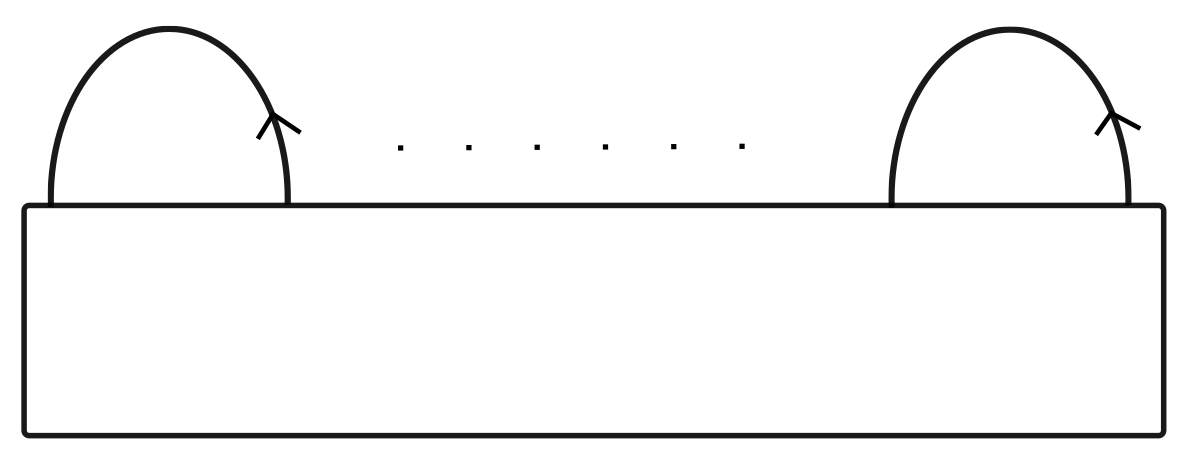
Figure 1. The ribbon graph $\Delta_{g}$, where all tangles are given the $0$-framing

Let $H_{g}$ be an oriented handlebody of genus $g$; we will assume that $H_{g}$ has one $0$-handle $D^{3}$ and $g$ $3$-dimensional $1$-handles all attached to the $0$-handle. Let $-H_{g}$ denote the handlebody $H_{g}$ with opposite orientation. We will fix our model of $\pm H_{g}$ to be a regular neighbourhood of $\pm\Delta_{g}$ in $S^{3}$, and we will fix $\partial(H_{g})=\Sigma_{g}$ as our model for a surface of genus $g$. Given an element $[f]\in\operatorname{\mathrm{Mod}}_{g,1}$ we can form the following closed $3$-manifold

$$S_{g}(f)=H_{g}\cup_{f}-H_{g}=H_{g}\sqcup\Sigma_{g}\times I\sqcup-H_{g}/\sim,$$

where $(x,0)\in\Sigma_{g}\times 0\sim x\in\partial(H_{g})$ and $(x,1)\in\Sigma_{g}\times 1\sim f(x)\in\partial(-H_{g})$. We will refer to the manifold $S_{g}(f)$ as a Heegaard splitting of genus $g$, and if the genus is clear from the context then we will abbreviate $S_{g}(f)$ to $S(f)$. There is an embedding of $\Sigma_{g}$ in this manifold given by $\partial(H_{g})$ that we refer to as the Heegaard surface.

Suppose we choose a framed link $L$ in $S^{3}-\pm\Delta_{g}$ such that Dehn surgery along $L$ produces $S(f)$ with $\pm\Delta_{g}$ embedded in $S^{3}\setminus L$ as in Figure 1. Then we get the ribbon graph $L\cup\Delta_{g}\cup-\Delta_{g}$ representing the manifold $S(f)$, which we think of as a Kirby diagram for $S(f)$ with added data. To get a framed link $L$ representing $S(f)$ in this way we begin by noting that $\#_{g}S^{1}\times S^{2}=S(\mathrm{id})$ has a surgery diagram given by $g$ disjoint unknots with framing $0$, and $H_{g},-H_{g}$ are given by tubular neighbourhoods of the copies of $\pm\Delta_{g}$ in Figure 2 .

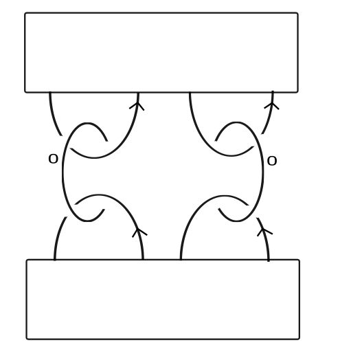
Figure 2. $\#_{g}S^{1}\times S^{2}=H_{g}\bigcup_{id}-H_{g}$ with $\pm\Delta_{g}$ embedded in them.

Take a positive normal to $\Sigma_{g}$ in $S^{3}$ and take an embedding of $\Sigma_{g}\times I$ into $S^{3}$ specified by this framing. Think of $\Sigma_{g}\times 0$ as $\partial(H_{g})$ and $\Sigma_{g}\times t$ as a pushoff of $\Sigma_{g}$ in the direction of the positive normal(pointing out of the page). Denote the image of this embedding of $\Sigma_{g}\times I$ into $S^{3}$ by $\nu(\Sigma_{g})$. We make sure that $\nu(\Sigma_{g})$ does not intersect any of the tangles in the diagram. Now we wish to modify the gluing map from $S(id)$ to $S(f)$ using the neighbourhood $\nu(\Sigma_{g})$.

Suppose we want to modify $S(id)$ using Dehn surgery to get $S(t_{c}^{i})$ for $i\in\{\pm 1\}$, where $c$ is a simple closed curve in $\Sigma_{g}\setminus D$. Pick a fiber $\Sigma_{g}\times\{pt\}:=F$ in $\nu(\Sigma_{g})$ and choose an embedding of $c$ in $F$, then let $A$ be an annular neighbourhood of $c$ in $F$ and write $N$ for the solid torus obtained by thickening $A$ to one side of $F$ in $\Sigma_{g}\times I\simeq\nu(\Sigma_{g})$. Now we remove $N$ and reglue it by the map of Figure 3; by construction this is Dehn surgery. Away from $N$ the fibering is the same, but as we pass across $N$ a Dehn twist about $c$ occurs. This changes the gluing from the identity to a Dehn twist about $c$. This Dehn surgery corresponds to adding a $4$-dimensional $2$-handle to the Kirby diagram with framing coefficient specified by the map of Figure 3.

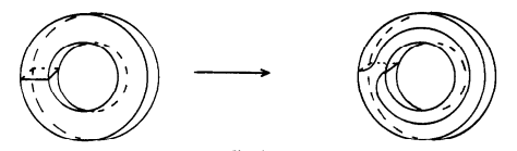
Figure 3. Figure taken from [Har82]

Next suppose we have $f$ written as a product of Dehn twists $t_{c_{n}}\cdot\cdot\cdot t_{c_{1}}$. Since $\nu(\Sigma_{g})=\Sigma_{g}\times I$, we pick $t_{1}<t_{2}<\cdot\cdot\cdot<t_{n}\in I$ and place the curve $c_{i}$ in the Kirby diagram at $\Sigma_{g}\times t_{i}$. Performing Dehn surgery along these curves by the map given by Figure 3 will give us $S(f)$. The framings on these curves in the Kirby diagram along with how these curves link will be captured by Seifert’s linking form, which will be described in the next section. An example of the tangle diagrams obtained from this method is given in Figure 4.

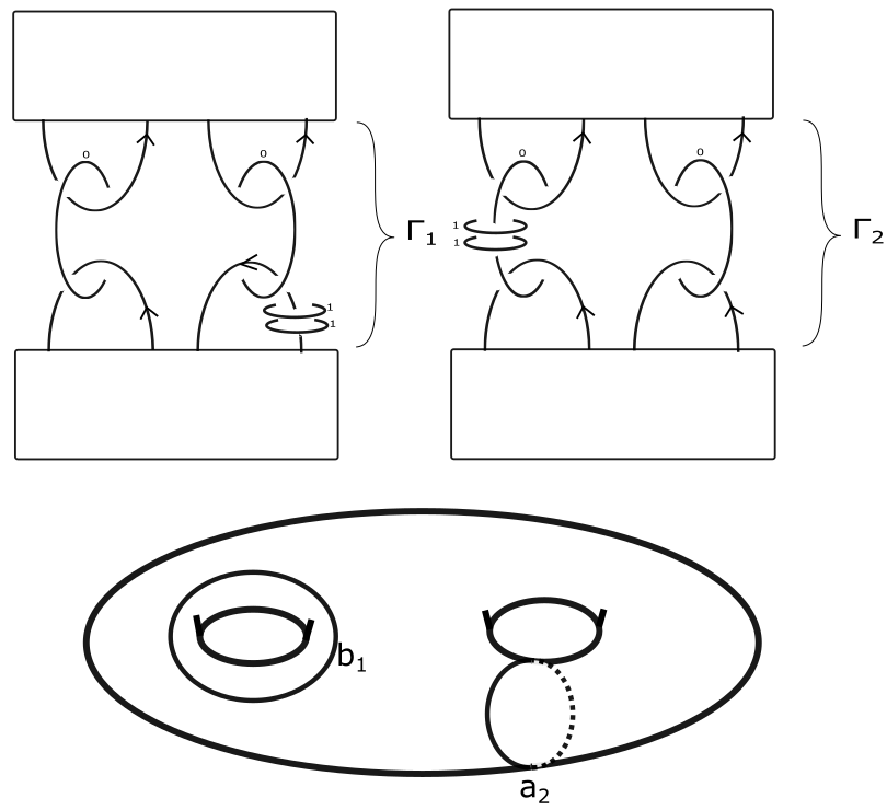
Figure 4. Tangle diagrams for $S(t_{a_{2}}^{2})$ (left) and $S(t_{b_{1}}^{2})$(right).

Now we explain how to go from the ribbon graphs of $S(f)$ described above to a framed link presentation of the mapping torus $M_{f}$. If we remove regular neighbourhoods $\nu(\pm\Delta_{g})$ in $S^{3}$ of the copies of $\pm\Delta_{g}$ in our ribbon graph for $S(f)$ we get a manifold diffeomorphic to $\Sigma_{g}\times I$ cut open along $\Sigma_{g}\times pt$ and reglued via $f$. So if we identify the remaining boundary surfaces via the identity we get $M_{f}$. Suppose we specify the manifold $S(f)$ by a ribbon graph in $S^{3}$ as above. Then identifying the two boundary surfaces is equivalent to adding a copy of $D^{1}\times H_{g}$ by gluing $-1\times H_{g}$ to $\nu(-\Delta_{g})$ and $1\times H_{g}$ to $\nu(\Delta_{g})$ in the Kirby diagram of the corresponding $2$-handlebody.

We assume that $H_{g}$ has one $0$-handle $D^{3}$, so we add one $4$-dimensional $1$-handle $D^{1}\times D^{3}$ to the Kirby diagram, along with $g$ $4$-dimensional $2$-handles $D^{1}\times D^{1}\times D^{2}$ coming from the $g$ $3$-dimensional $1$-handles of $H_{g}$. These $4$-dimensional $2$-handles are attached with framing $0$ (draw the relevant portion $\partial(D^{1}\times D^{1})\times\{pt\}$ for $pt\in\partial D^{2}$ that is visible in the Kirby diagram). This gives us a Kirby diagram for a $4$-manifold with boundary $M_{f}$.

Now we think of the two $3$-balls $\partial{D}^{1}\times D^{3}$ of the $4$-dimensional $1$-handle attached in Figures 2, 4 as tubular neighbourhoods of the coupons of $\pm\Delta_{g}$ in $S^{3}$. The $4$-dimensional $2$-handles are given by the tangles attached to the coupons (these $2$-handles run over the $1$-handle). Here the endpoints of the strands of the tangle of the bottom coupon are identified with the endpoint of the strand of the tangle of the top coupon which is directly above it. We call the corresponding $4$-manifold given by this Kirby diagram $X_{f}$.

Seifert pairing

Suppose that an oriented surface $F$ has been embedded in $S^{3}$; given a curve $a$ on $F$ representing a cycle, let $a^{+}$ denote the pushoff of $a$ in the direction of the positive normal to $F$. We define Seifert’s linking pairing

$$\lambda:H_{1}(F;\mathbb{Z})\times H_{1}(F;\mathbb{Z})\rightarrow\mathbb{Z}$$

by the formula $\lambda(a,b)=lk(a,b^{+})$. It turns out that $\lambda$ is a well-defined bilinear pairing and is an invariant of the ambient isotopy class of the embedding of $F$ into $S^{3}$. (See [Kau87, Chapter VII] for more details). Note that in our setup we orient $S^{3}$ and $F$ so that the positive normal points out of the page, toward the reader.

On the boundary, attaching a $4$-dimensional $2$-handle with framing $n$ along a knot $K$ is equivalent to removing a solid torus neighbourhood of $K$ and gluing a solid torus back in by sending a meridian to the pushoff $K^{\prime}$ of $K$ in the direction of the transverse vector field of the framing.

For a curve $c$ on a surface $F$ embedded in $S^{3}$, the self-linking form $\lambda(c,c)$ can be computed by $lk(c,c^{*})$, where $c^{*}$ is a parallel copy of $c$ along the surface $F$. We want to remove a torus neighbourhood of $c$ and reglue by the map of Figure 3 and the discussion above implies that this is equivalent to attaching a $4$-dimensional $2$-handle along $c\subset F$ with framing $\lambda(c,c)\pm 1$, where the $\pm 1$ comes from the gluing being $t_{c}^{\pm 1}$.

3.1. Dotted circle notation

We are now able to find the Kirby diagram of a $4$-manifold with the boundary being $M_{f}$, where $f:\Sigma_{g}\rightarrow\Sigma_{g}$ is a diffeomorphism. Next we will describe dotted circle notation, due to Akbulut [Akb77].

If we smooth corners so that $D^{2}\times D^{2}=D^{4}$ we have a diffeomorphism $(D^{2}\setminus\nu\{0\})\times D^{2}=(S^{1}\times D^{1})\times D^{2}=S^{1}\times D^{3}$, where $\nu\{0\}$ is a tubular neighbourhood of $0\in D^{2}$. From this we see that adding a $1$-handle is the same as removing an open tubular neighbourhood of a properly embedded $2$-disc $\{0\}\times D^{2}$, whose boundary $\{0\}\times\partial D^{2}$ is visible in the Kirby diagram as a dotted circle as in Figure 5.

The $\nu\{0\}\times\partial D^{2}$ part of the tubular neighbourhood is visible in $\partial D^{4}=S^{3}$ as a solid torus and the annulus $(D^{2}\setminus\nu\{0\})\times\{pt\}$ allows us to isotope a curve running through the $1$- handle to $\partial\nu\{0\}\times pt$, which links once with the removed solid torus in $\partial D^{4}$.

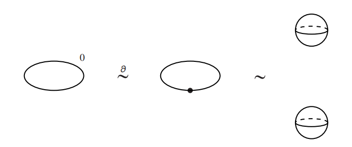
Figure 5. Figure taken from [GS99] Section 5.4

Note that $\partial(S^{1}\times D^{3})=S^{1}\times S^{2}=\partial(D^{2}\times S^{2})$, where the Kirby diagram of $D^{2}\times S^{2}$ is given by a $0$-framed unknot. Moving from the dotted circle to the $0$-framed unknot as in Figure 5 is done via surgery in the interior of the $4$-manifold, and the symbol $\overset{\partial}{\sim}$ denotes that there is a diffeomorphism between the two boundary $3$-manifolds.

Given a Kirby diagram with $1$-handles, we can switch to dotted circle notation by isotoping the attaching circles of any $2$-handles so that they avoid the regions between the attaching balls of the $1$-handles. Then we can push the balls together and switch to dotted circle notation. In doing this we must remember that curves running through the $4$-dimensional $1$-handle are linked with the dotted circle and are joined together by the gluing data of the $4$-dimensional $1$-handles. We will use the convention of drawing dotted lines to indicate the paths taken to push any balls together (For more information see [GS99, Section 5.4]). Applying this operation to the Kirby diagram of the $4$-manifold $X_{f}$ we have found with $\partial X_{f}=M_{f}$, then changing the dotted circles to $0$-framed unknots gives us a surgery diagram for $M_{f}$. The framings are well-defined once we have drawn the dotted lines.

Note that there is a natural way to switch to dotted circle notation using the ribbon graphs above; we simply push the two balls given by the coupons together along a dotted line running to the right. An example is given by Figure 6.

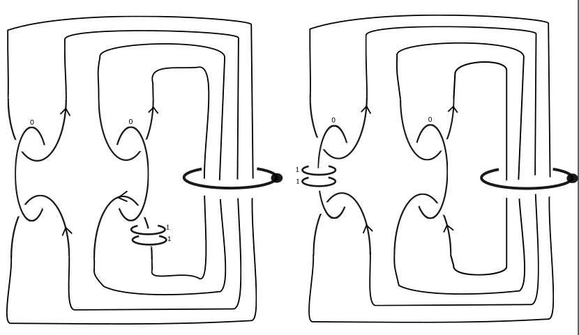
Figure 6. Surgery diagrams for $M_{t_{a_{2}}^{2}}$ and $M_{t_{b_{1}}^{2}}$ obtained from Figure 4

Surgery diagrams from composing tangles

We can also construct surgery diagrams for mapping tori by concatenating tangle diagrams; this will be useful later on for showing that Sato’s maps $\beta_{\sigma}$ are in fact homomorphisms.

Recall that we can think of the ribbon graphs obtained as in Figure 4 as surgery diagrams for $S(f)\coloneqq H_{g}\bigcup_{f}-H_{g}$ if we surger along the closed components of the tangle diagram. The handlebodies $\pm H_{g}$ are viewed as tubular neighbourhoods in $S^{3}$ of the $\pm\Delta_{g}$. This breaks $S(f)$ into three pieces, $\nu(\pm\Delta_{g})$ and a copy of $\Sigma_{g}\times I$ cut open along a $\Sigma_{g}\times\{pt\}$ and reglued via $f$. If we remove tubular neighbourhoods in $S^{3}$ of the $\pm\Delta_{g}$ we get tangle diagrams for the relevant mapping cylinders $C_{f}=\Sigma_{g}\times I\bigsqcup\Sigma_{g}/\sim$ where $(x,1)\sim f(x)$. Given such a ribbon graph of $S(f)$ corresponding to $C_{f}$, we denote by $\Gamma_{f}$ the tangle diagram obtained by deleting the top and bottom coupons. The following useful result is due to Reshetikhin-Turaev [RT91, Lemma 4.4].

Lemma 3.1.

Let $\Gamma_{f},\Gamma_{g}$ be two tangle diagrams as above representing $C_{f},C_{g}$. Then the composition $\Gamma_{f}\circ\Gamma_{g}$ obtained by stacking $\Gamma_{f}$ on top of $\Gamma_{g}$ and then putting coupons on the ends gives a ribbon graph for $S(f\circ g)$.

In Lemma 3.1 the unknotted components coming from the tangles with endpoints on the coupons are given the $0$-framing. After composing the tangle diagrams and putting coupons on the two opposite ends, the resulting copies of $\pm\Delta_{g}$ in our ribbon graph have regular neighbourhoods in $S^{3}$ corresponding to $\pm H_{g}$. Removing these copies of $\pm H_{g}$ gives us the mapping cylinder $C_{f\circ g}$ so the ribbon graph obtained gives a surgery diagram for $S(f\circ g)$.

For example the tangle diagram for $C_{t_{a_{2}}^{2}t_{b_{1}}^{2}}$ given in Figure 7 is obtained using the tangle diagrams for $C_{t_{a_{2}}^{2}}$ and $C_{t_{b_{1}}^{2}}$ given in Figure 4. Now, thinking of the coupons attached to $\Gamma_{t_{a_{2}}^{2}t_{b_{1}}^{2}}$ as $4$-dimensional $1$-handles again and changing to dotted circle notation gives a surgery diagram for $M_{t_{a_{2}}^{2}t_{b_{1}}^{2}}$.

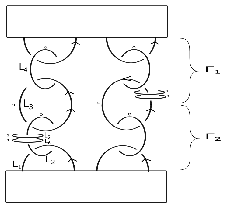
Figure 7. Another surgery diagram for $M_{t_{a_{2}}^{2}t_{b_{1}}^{2}}$, obtained by concatenating the tangles of Figure 4

4. Rewriting Sato’s maps

From now on we write $M_{L}$ for the $3$-manifold obtained via Dehn surgery on the oriented, framed link $L$ in $S^{3}$, and we assume that $M_{L}$ is diffeomorphic to the mapping torus $M_{\varphi}$. We denote by $W_{L}$ the corresponding $2$-handlebody with Kirby diagram given by the framed link $L$. The linking matrix of $L$ is also the matrix of the intersection form of $W_{L}$ with respect to the basis given by the components $L_{i}$ of $L$. We use the symbol $\cdot$ to denote this intersection form.

4.1. Rewriting the map $\theta:\operatorname{\mathrm{Spin}}(\Sigma_{g})\rightarrow\operatorname{\mathrm{Spin}}(M)$

The aim of this section is to rewrite the map $\theta$ so that it outputs a framed link diagram for the mapping torus, along with a characteristic sublink (defined below). This allows us to evaluate the Rochlin invariant of a given spin structure from the link diagram. To do this we first describe two ways in which spin structures can be defined for a $3$-manifold given by a surgery diagram.

First note that since $H^{1}(S^{1})\cong\mathbb{Z}/2$, we have that for a knot $\gamma$ in $S^{3}$ there are two homotopy classes of spin structures on $\gamma$. One is the bounding spin structure induced by the unique spin structure on $D^{2}$, the other is the Lie group structure. If we use the correspondence given above between framings and linking number, it turns out that the Lie group structure corresponds to the $0$-framing.

Suppose the framed link $L$ has $n$ components, let $L_{i}$ denote a component and let $p_{i}$ denote the framing coefficient of $L_{i}$. Suppose we fix an orientation of $L$ and let the pairs $(\mu_{i},\lambda_{i})$ denote a choice of right-handed meridian and $0$-framed longitude for $L_{i}$. We have that $H_{1}(S^{3}\setminus L;\mathbb{Z})\simeq\mathbb{Z}^{n}$ with generators being the $\mu_{i}$ and $H_{1}(M_{L};\mathbb{Z})$ is a quotient of $H_{1}(S^{3}\setminus L;\mathbb{Z})$ by the relations

$$p_{i}\mu_{i}+\lambda_{i}=p_{i}\mu_{i}+\sum_{j\neq i}lk(L_{i},L_{j})\mu_{j}=0.$$

In the splitting $H_{1}(M_{L})=H_{1}(\Sigma_{g})\bigoplus H_{1}(S^{1})$ given by the exact sequence (2), we see that we can represent a basis for the $H_{1}(\Sigma_{g})$ factor of $H_{1}(M_{L})$ by placing the canonical curves of the basis for $H_{1}(\Sigma_{g})$ in a fiber. Comparing with our diagram for $S^{1}\times\Sigma_{g}$ coming from Figure 2, these curves go to meridians of the components in our fixed diagram. A curve representing a generator for the $H_{1}(S^{1})$ factor given by the embedding $l:D\times S^{1}\rightarrow M_{\varphi}=M_{L}$ goes to a meridian of the $0$-framed unknot component coming from the dotted circle. Here we always join the two $3$-balls together along a dotted line running to the right of the tangle diagram.

For $\sigma\in\operatorname{\mathrm{Spin}}(\Sigma_{g})$, we have that $\theta(\sigma)$ is a right splitting of the short exact sequence

(5) $$0\rightarrow H_{1}(SO(3))\overset{i}{\rightarrow}H_{1}(P(M_{L}))\overset{p}{\rightarrow}H_{1}(M_{L})\rightarrow 0$$

of the oriented frame bundle of $M_{L}$, and under the splitting of $H_{1}(M_{L})$ it is given by $\sigma\oplus\hat{l}$. We can equivalently think of a spin structure as a trivialization over the $1$-skeleton that extends over the $2$-skeleton, and by functoriality any such trivialization will give a right splitting of (5). So we can think of $\sigma\oplus\hat{l}$ as framing the canonical curves in the basis for $H_{1}(M_{L})$. For any $\widetilde{b}\in H_{1}(P(M_{L}))$ we have that $\widetilde{b}=(\widetilde{b}-\sigma\oplus\hat{l}(p(\widetilde{b})))+\sigma\oplus\hat{l}(p(\widetilde{b}))$ with $\widetilde{b}-\sigma\oplus\hat{l}(p(\widetilde{b}))\in\operatorname{\mathrm{ker}}(p)=\operatorname{\mathrm{im}}(i)=\mathbb{Z}/2$. So this sum realises the splitting of $H_{1}(P(M_{L}))$ into $H_{1}(SO(3))\bigoplus H_{1}(M_{L})$.

Think of $\widetilde{b}\in H_{1}(P(M_{L}))$ as a framed curve $b$ in $M_{L}$, then the map
$k_{\theta(\sigma)}:H_{1}(P(M_{L}))\rightarrow H_{1}(SO(3))=\mathbb{Z}/2$ given by

$$k_{\theta(\sigma)}(\widetilde{b})=\widetilde{b}-\sigma\oplus\hat{l}(p(\widetilde{b}))$$

is a left splitting of (5). By homotopy invariance of homology we have that $k_{\theta(\sigma)}(\widetilde{b})$ is $0$ if the homotopy class of the framing given by $\widetilde{b}$ agrees with the homotopy class of the framing of $b$ given by the spin structure, and is $1$ otherwise. We also have that $k_{\theta(\sigma)}(i(1))=1$ always and $i(1)$ can be thought of as an unknot in $M_{L}$ with $0$-framing (Lie group framing).

We have a smooth map $\mathrm{inc}:P(S^{3}\setminus L)\rightarrow P(M_{L})$ induced by the inclusion of $S^{3}\setminus L$ into $M_{L}$ that induces a homomorphism $\mathrm{inc}*:H^{1}(P(M_{L}))\rightarrow H^{1}(P(S^{3}\setminus L))$. As noted in Section $3$, the oriented core of the torus surgered along $L_{i}$ is always a negatively oriented meridian $\mu_{i}$ of $L_{i}$. Suppose we give this meridian the framing induced from the product framing on the $2$-handle in $W_{L}$ attached along $L_{i}$, call it $\widetilde{\mu_{i}}$. Then we have that $\mathrm{inc}*(k_{\theta(\sigma)}(\widetilde{\mu_{i}}))=k_{\theta(\sigma)}(\mathrm{inc}(\widetilde{\mu_{i}}))$ is $0$ if the spin structure extends across the $2$-handle in $W_{L}$ attached along $L_{i}$, and is $1$ otherwise. In other words $k_{\theta(\sigma)}(\mathrm{inc}(\widetilde{\mu_{a}}))$ is $0$ if the spin structure $\theta(\sigma)$ extends over $L_{i}$ and is $1$ otherwise.

Let $\mu_{0}$ be the meridian of the $0$-framed unknot which came from the dotted circle; in Sato’s construction of $\theta(\sigma)$ we have that $\sigma\oplus\hat{l}(\mu_{0})$ has been framed using $\hat{l}$ which corresponds to $1$ under linking number. We will always set $\mathrm{inc}*(k_{\theta(\sigma)})(\mu_{0})=0$. Now we relate this construction purely to cohomology classes of $S^{3}\setminus L$.

Spin structures on $S^{3}\setminus L$ are classified by $H^{1}(S^{3}\setminus L)=\operatorname{\mathrm{Hom}}(H_{1}(S^{3}\setminus L;\mathbb{Z}),\mathbb{Z}/2)$, where we choose the zero element to correspond to the restriction of the unique spin structure on $S^{3}=\partial D^{4}$ to $S^{3}\setminus L$. By our description above, $\omega\in\operatorname{\mathrm{Hom}}(H_{1}(S^{3}\setminus L;\mathbb{Z}),\mathbb{Z}/2)$ is completely determined by its values on the $\mu_{i}$. We will also have that $\omega(\mu_{i})=0$ if and only if the spin structure given extends over the $2$-handle in $W_{L}$ attached along $L_{i}$.

For the following correspondence see [FFU01, Proposition 1].

Proposition 4.1.

There is a bijective correspondence between spin structures on $M_{L}$ and elements $\omega\in\operatorname{\mathrm{Hom}}(H_{1}(S^{3}\setminus L;\mathbb{Z}),\mathbb{Z}/2)$ satisfying the following relations

$$p_{i}\omega(\mu_{i})+\sum_{j\neq i}lk(L_{i},L_{j})\omega(\mu_{j})=p_{i}\pmod{2},$$

for $1\leq i\leq n$.

To determine a spin structure on a surface, it is enough to specify which simple closed curves in a canonical basis are spin bounding and which are not (see [Joh80a]). Using the canonical basis placed in the Kirby diagram and the discussion above, this translates to defining an $\omega\in\operatorname{\mathrm{Hom}}(H_{1}(S^{3}\setminus L;\mathbb{Z}),\mathbb{Z}/2)$ by setting its values to be either $0$ or $1$ on the meridians of the components of our fixed diagram for $\Sigma_{g}\times S^{1}$ coming from Figure 2. We will always set $\omega(\mu)=0$ for $\mu$ being the meridian of the $0$-framed component coming from the dotted circle. The correspondence in Proposition 4.1 gives us relators which we can use to deduce what the values of $\omega$ must be on the meridians of the components coming from modifying the monodromy of the mapping torus. These relations are enough because if $c$ is one such component, we cannot have that $c$ links evenly with every other component, as then $c$ would represent a non-primitive homology class in the fiber surface, contradicting the fact that $c$ is simple.

This description rewrites $\theta$ as a map $\operatorname{\mathrm{Spin}}(\Sigma_{g})\rightarrow\operatorname{\mathrm{Hom}}(H_{1}(S^{3}\setminus L;\mathbb{Z}),\mathbb{Z}/2)$.

Now we describe how to go from $\operatorname{\mathrm{Hom}}(H_{1}(S^{3}\setminus L;\mathbb{Z}),\mathbb{Z}/2)$ to a characteristic sublink in the link diagram. We begin by defining a characteristic sublink.

Definition 4.2.

For a $3$-manifold $M_{L}$, a sublink $C$ of $L$ is called characteristic if $C\cdot L_{i}=L_{i}\cdot L_{i}\pmod{2}$ for all components $L_{i}$ of $L$.

There is a bijective correspondence between the spin structures on $M_{L}$ and the characteristic sublinks of $L$ (see [KM91] Appendix C for a proof). The correspondence is given by taking a spin structure $s$ of $M_{L}$ and defining the sublink $C$ of $L$ to consist of all components $L_{i}$ of $L$ such that the spin structure $s$ does not extend over the $2$-handle in $W_{L}$ attached to $L_{i}$.

We noted just before Proposition 4.1 that for any $\sigma\in\operatorname{\mathrm{Spin}}(\Sigma_{g})$,
$\theta(\sigma)\in\operatorname{\mathrm{Hom}}(H_{1}(S^{3}\setminus L;\mathbb{Z}),\mathbb{Z}/2)$ has the property that $\theta(\sigma)(\mu_{i})=0\mod 2$ if and only if the spin structure extends over $L_{i}$. So we define the associated characteristic sublink of $L$ to be all components $L_{i}$ of $L$ such that $\theta(\sigma)(\mu_{i})=1\pmod{2}$.

One way to see this is to note that if we take the components with $\theta(\sigma)(\mu_{i})=1\pmod{2}$ and plug into the relators of Proposition 4.1, we are simply writing out the defining condition of a characterstic sublink. This map

$$\operatorname{\mathrm{Hom}}(H_{1}(S^{3}\setminus L;\mathbb{Z}),\mathbb{Z}/2)\rightarrow\{\mathrm{Characteristic\>sublinks\>of\>L}\}$$

allows us to rewrite $\theta$ as a map

$$\theta:\operatorname{\mathrm{Spin}}(\Sigma_{g})\rightarrow\{\mathrm{Characteristic\>sublinks\>of\>L}\}.$$

Summary

We take a collection of simple closed curves $a_{1},b_{1},...,a_{g},b_{g}$ representing a basis for the fiber homology and assign these curves values in $\{0,1\}$ to get $\sigma\in\operatorname{\mathrm{Spin}}(\Sigma_{g})$. These curves $a_{i},b_{i}$ go to meridians of components $L_{a_{i}},L_{b_{i}}$ in our surgery diagram and $\theta(\sigma)$ is the union of all the components whose corresponding curves were assigned the value $1$. The relation of Proposition 4.1 then finds the full characteristic sublink.

Note that the action of $H^{1}(\Sigma_{g})$ on $\operatorname{\mathrm{Spin}}(\Sigma_{g})$ is by function addition, and in our setup this corresponds to changing the values of $\theta(\sigma)$ on the meridians of the components present in our diagram for $\Sigma_{g}\times S^{1}$. In other words suppose $a$ is a simple closed curve representing a basis vector in $H_{1}(\Sigma_{g})$ in the fiber, which goes to a meridian of a closed component $L_{a}$ in our diagram. Suppose that $x\in H^{1}(\Sigma_{g})$ has $x([a])=1$, then for the characteristic sublink $\theta(\sigma+x)$ we switch whether $L_{a}\in\theta(\sigma+x)$. We then have to use the relations in Proposition 4.1 to deduce how the values change on the meridians of the components associated with the monodromy.

Remark on well-definedness

Note that we have two methods for finding the surgery diagram of a mapping torus $M_{f}$ where $f$ is a product of squares of Dehn twists. One is to simply modify the monodromy by Dehn surgery in a single tubular neighbourhood $\Sigma_{g}\times I$ of the Heegaard surface. An example of this was given by starting from Figure 2 and adding pushoffs of curves on the Heegaard surface to modify monodromy from the identity to $f\in\operatorname{\mathrm{Mod}}_{g,1}[2]$ as in Figure 8. The other method for describing the mapping torus is to use Lemma 3.1 and compose tangle diagrams individually to get a surgery diagram as in Figure 7. Suppose we denote by $\Gamma_{f},\Gamma_{g}$ two tangle diagrams representing $M_{f}$ and $M_{g}$ respectively, where $f$ and $g$ are squares of Dehn twists. The concatenation $\Gamma_{f}\circ\Gamma_{g}$ represents $M_{f\circ g}$ and for the framed link presentations from both methods, we have a fixed embedding of a surface into $S^{3}$ representing the fiber, and a fixed embedding for the dotted circle component. So we can use our map $\theta$ on both diagrams. It does not matter which method we choose since both diagrams with the characteristic sublinks given by $\theta(\sigma)$ are spin diffeomorphic. This can be seen using Kirby calculus, and keeping track of how the characteristic sublink changes as in [KM91, Appendix C, Moves 1 and 2] [MP94, Fig. 3 (K3 move)]; an example for genus $1$ is given in Figure 9. This argument can be generalised as in Figure 10; isotope the components corresponding to Dehn twists so that they lie as in Figure 10, then slide each strand over $L^{\prime}$. There are an even number of strands so the characteristic sublink changes accordingly, then use [MP94, K3 move]. The same argument works for concatenating tangle diagrams of $\Gamma_{f}$, where $f$ is a bounding pair map or a separating twist (see Section $5$).

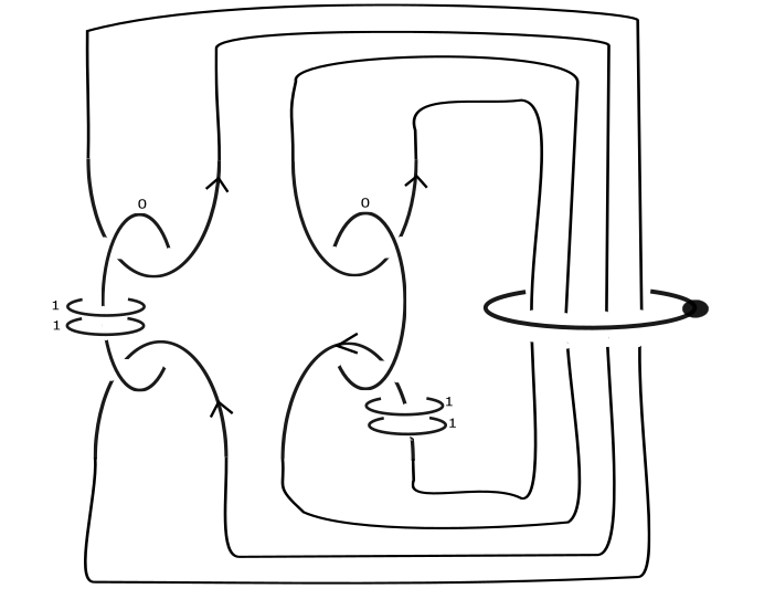
Figure 8. A surgery diagram for $M_{t_{a_{2}}^{2}t_{b_{1}}^{2}}$, where $a_{2}$ and $b_{1}$ are the curves of Figure 4

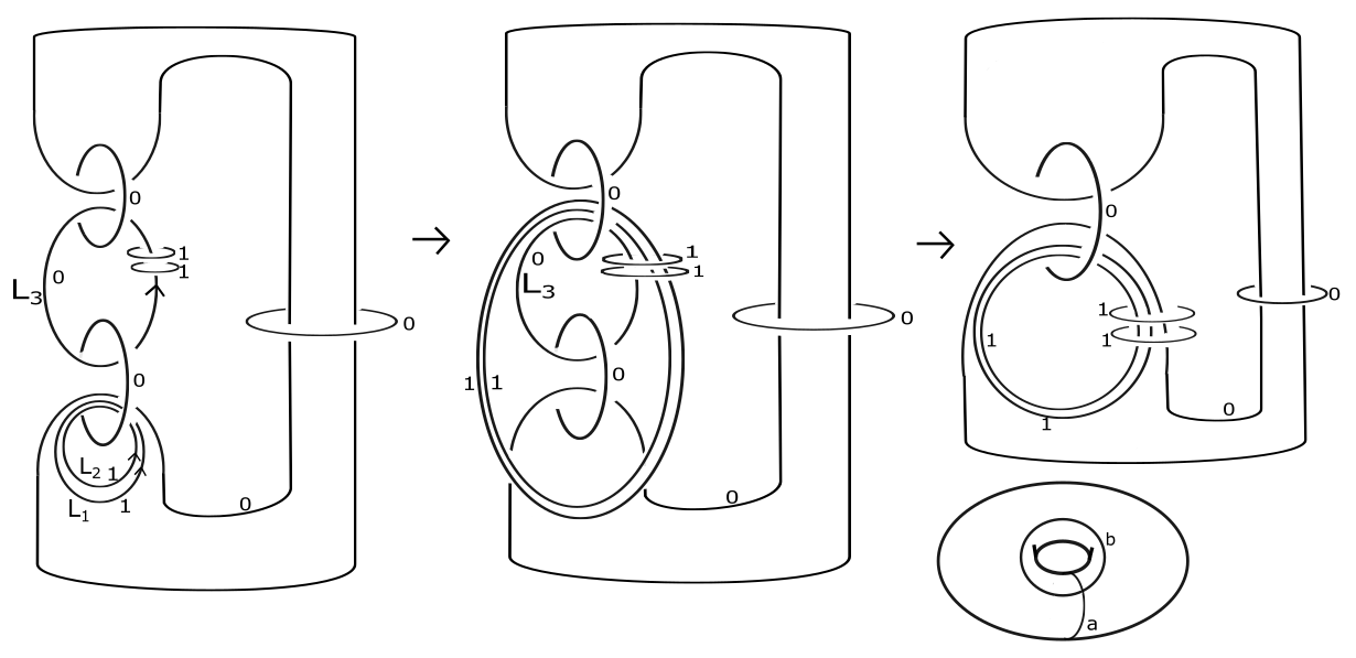
Figure 9. Two (spin)-diffeomorphic surgery diagrams for $M_{t_{a}^{2}t_{b}^{2}}$. The first move is to slide the components $L_{1},L_{2}$ corresponding to $t_{b}^{2}$ over $L_{3}$. Since they come in pairs, the characteristic sublink changes accordingly. The second move is [MP94, K3 move]. A similar argument works for diagrams of $M_{t_{b}^{2}t_{a}^{2}}$; the order of concatenation matters.

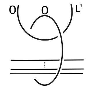
Figure 10. General case.

4.2. $\beta_{\sigma}$ is a homomorphism

Now we give a proof that Sato’s maps

$$\beta_{\sigma}:\operatorname{\mathrm{Mod}}_{g,1}[2]\rightarrow\operatorname{\mathrm{Map}}(H_{1}(\Sigma_{g}),\mathbb{Z}/8)$$

are in fact homomorphisms by using a formula for computing the Rochlin invariant from a surgery diagram with a labelled characteristic sublink. The proof will make it intuitively clear why it is a homomorphism on the subgroup generated by squares of Dehn twists.

From now on we will think of $\theta$ as a map from $\operatorname{\mathrm{Spin}}(\Sigma_{g})$ to framed links $(L,C)$ such that $(M_{L},C)$ is spin diffeomorphic to $(M_{\varphi},\theta(\sigma)$), where these links $(L,C)$ are obtained using the methods of Section $3$. We can write the Rochlin invariant of $M_{L}$ with spin structure corresponding to $\theta(\sigma)$ as

(6) $$R(M_{L},\theta(\sigma))=\Lambda_{L}-\theta(\sigma)\cdot\theta(\sigma)+8\operatorname{\mathrm{Arf}}(\theta(\sigma))\pmod{16}.$$

In this formula $\Lambda_{L}$ is the signature of the linking matrix of $L$, $\theta(\sigma)\cdot\theta(\sigma)$ is the sum of all the entries in the linking matrix of the characteristic sublink of $\theta(\sigma)$, and $\operatorname{\mathrm{Arf}}(\theta(\sigma))\in\{0,1\}$ is the Arf invariant of the characteristic sublink of $\theta(\sigma)$, which we now define (see [KM91, (C.3), Corollary C.5]).

The Arf invariant of a proper link

We will call a link $L$ proper if $lk(K,L-K)$ is even for every component $K$ of $L$. For any proper link $L$ we will say that the knot $K$ is related to $L$ if there exists a smoothly and properly embedded disk with holes $D$ in $S^{3}\times I$ with $D\cap(S^{3}\times\{0\})=K$ and $D\cap(S^{3}\times\{1\})=-L$. We define the Arf invariant $\operatorname{\mathrm{Arf}}(L)$ of $L$ to be the standard Arf invariant in $S^{3}$ of any knot $K$ related to $L$ (See [Rob65] or [Hos84] for more details). One point to note is that for a proper link $L$, we can produce a knot $K$ related to $L$ by just band connecting together all the components of $L$, as long as the bands respect the orientations chosen for the components of $L$. This can be seen by taking $L\times I$; the band sum corresponds joining the boundary components of the disjoint annuli at one end by bands to get a disk with holes.

Let $F$ be Seifert surface for $L$, and let $i:L\rightarrow\partial F$ denote the inclusion. Then $\operatorname{\mathrm{im}}(i_{*})$ is the radical of the intersection form on $H_{1}(F)$ and the Seifert self linking form $\lambda:H_{1}(F)\rightarrow\mathbb{Z}/2$ satisfies $\lambda|_{\operatorname{\mathrm{im}}(i_{*})}=0$ if and only if $L$ is a proper link. We can also define $\operatorname{\mathrm{Arf}}(L)$ to be the Arf invariant of the form on $H_{1}(F)/\operatorname{\mathrm{im}}(i_{*})$ induced by $\lambda$.

Another definition of Sato’s maps

Plugging formula (6) into Sato’s definition of the homomorphisms, we get

(7) $$\beta_{\sigma,x}([\varphi])=(\theta(\sigma+x)\cdot\theta(\sigma+x)-\theta(\sigma)\cdot\theta(\sigma)+8(\operatorname{\mathrm{Arf}}(\theta(\sigma))-\operatorname{\mathrm{Arf}}(\theta(\sigma+x))))/2\pmod{8}$$

We can take the above formula as another definition of $\beta_{\sigma,x}$ (see [KM91, Theorem C.4]). The fact that this is a spin diffeomorphism invariant means that it is invariant under changing the orientations of the individual components of any framed link diagram representing $M_{\varphi}$. We will often choose orientations so as to simplify calculations for the linking matrix sum in the above formula; examples of these orientation choices are given in Sections $4.3$ and $5$.

By our description of $\theta$ from the previous section a spin structure for these surgery diagrams is given by specifying which simple closed curves in the standard basis for the homology of this fiber surface are spin bounding and which are not. For Figures 8 and 7 the standard curves $a_{1},b_{1}$ for the genus part on the bottom left go to meridians of the components $L_{1},L_{2}$ respectively. So giving this diagram a spin structure is equivalent to declaring whether or not $L_{1},L_{2}$ are in the characteristic sublink (and doing so for all holes in $\Delta_{g}$). As before we then use the relations in Proposition 4.1 to find the full characteristic sublink. We declare that the dotted circle component is never in the characteristic sublink when defining our map $\theta:\operatorname{\mathrm{Spin}}(\Sigma_{g})\rightarrow\operatorname{\mathrm{Spin}}(M_{t_{a_{2}}^{2}t_{b_{1}}^{2}})$.

Lemma 4.3.

Sato’s maps $\beta_{\sigma}:\operatorname{\mathrm{Mod}}_{g,1}[2]\rightarrow\operatorname{\mathrm{Map}}(H_{1}(\Sigma_{g}),\mathbb{Z}/8)$ are homomorphisms.

Proof.

We will prove that $\beta_{\sigma}(t_{b}^{2}t_{a}^{2})=\beta_{\sigma}(t_{b}^{2})+\beta_{\sigma}(t_{a}^{2})$. The general proof will follow by induction on word length with respect to the generating set of squares of Dehn twists, with the inductive step given below. We illustrate the proof by example; the basic idea is that the characteristic sublink obtained from $\theta$ in Figure 7 is almost the union of the characteristic sublinks given by $\theta$ in Figure 4.

To find the characteristic sublink in Figure 7 we use the relations

(8) $$w\left(p_{i}\mu_{i}+\sum_{i\neq j}lk(L_{i},L_{j})\mu_{j}\right)=p_{i}\pmod{2}$$

of Proposition 4.1. We note that the surgery curves coming from the Dehn twist factorisation come in pairs and since they are isotopic on the Heegaard surface and have the same framing, the relations imply they are either both in, or both out of the characteristic sublink. But then using the relations of (8) for $i=2$ in Figure 7 imply that $w(\mu_{1})=w(\mu_{3})$, similarly using (8) for $i=3$ imply $w(\mu_{2})=w(\mu_{4})$. Doing so for all genus parts of the tangle diagram implies that the components for $\theta(\sigma)$ in Figure 7 which come from the Dehn twist factorisation is just the disjoint union of the charactersitic sublinks for $\theta(\sigma)$ coming from the two diagrams of Figure 4.

Now write all the diagrams given by Figures 4 and 7 in dotted circle notation (keeping in mind we have set the dotted circle to never be in $\theta(\sigma)$). After doing the band sums indicated in Figure 11 we see that $\theta(\sigma)\cdot\theta(\sigma)$ for Figure 7 is just the sum of the two $\theta(\sigma)\cdot\theta(\sigma)$ coming from the surgery diagrams of Figure 4. This follows because in our framed link diagrams, the components which pass through the dotted circle all have framing zero.

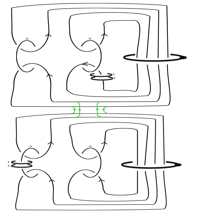
Figure 11.

Figure 12.

Comparing this with the surgery diagram of Figure 12 (where dotted path indicates how to join the $3$-balls to form the dotted circle), we see that after band summing we have same diagram as the one obtained for $M_{t_{b_{1}}^{2}t_{a_{2}}^{2}}$ except with one additional dotted circle. The fact that $\beta_{\sigma}$ is a homomorphism then follows from the fact that $\operatorname{\mathrm{Arf}}(L_{1}\cup L_{2})=\operatorname{\mathrm{Arf}}(L_{1})+\operatorname{\mathrm{Arf}}(L_{2})$ for the disjoint union of $L_{1}$ and $L_{2}$ and the fact that the Arf invariant can be calculated by band summing the components. ∎

4.3. Evaluation on squares

We can now use our definition to give a formula for $\beta_{\sigma}$ on squares of Dehn twists on nonseparating curves analogous to that of Sato’s [Sat10, Proposition 5.2].

Corollary 1.

Let $c$ be a nonseparating simple closed curve in $\Sigma_{g,1}$ then we have that

$$\beta_{\sigma,x}(t_{c}^{2})=\left\{\begin{array}[]{ll}0,&c_{1}\cup c_{2}\in\theta(\sigma)\>\mathrm{and}\>\in\theta(\sigma+x)\\ 0,&c_{1}\cup c_{2}\notin\theta(\sigma)\>\mathrm{and}\>\notin\theta(\sigma+x)\\ 1,&c_{1}\cup c_{2}\in\theta(\sigma+x)\>\mathrm{and}\>\notin\theta(\sigma)\\ -1,&c_{1}\cup c_{2}\in\theta(\sigma)\>\mathrm{and}\>\notin\theta(\sigma+x),\end{array}\right.$$

where $c_{1}$ and $c_{2}$ are pushoffs of $c$ in the fiber surface, framed using the Seifert pairing, and $c_{i}\in\theta(\sigma)$ denotes that $c_{i}$ is in the characteristic sublink.

Proof.

We take the Seifert linking form $\lambda$ for the fiber surface $\Sigma_{g,1}$ visible in the Kirby diagram as in Figure 6 and set $m=\lambda(c,c)$. Note that by our construction we can take the components $L_{c_{1}}$ and $L_{c_{2}}$ corresponding to the monodromy to lie on the same fiber surface, isotoped to be disjoint from each other. We orient these components oppositely on the fiber surface.

Now we recall the formula for $\beta_{\sigma,x}$ given in (7)

$$\beta_{\sigma,x}([\varphi])=(\theta(\sigma+x)\cdot\theta(\sigma+x)-\theta(\sigma)\cdot\theta(\sigma)+8(\operatorname{\mathrm{Arf}}(\theta(\sigma))-\operatorname{\mathrm{Arf}}(\theta(\sigma+x))))/2\pmod{8}.$$

To calculate the Arf invariant terms note that since $c_{1}$ and $c_{2}$ are isotopic and oppositely oriented they bound an annulus on the fiber surface. Since they are isotopic the formula of Proposition 4.1 implies that $L_{c_{1}}$ and $L_{c_{2}}$ are either both in or both out of the characteristic sublink for any spin structure. Suppose they are both in, then we can band sum in this annulus to get an unknot disjoint from the rest of the characteristic sublink. If we compare with Figure 6 we see that in any case, after band summing we have a disjoint union of unknots (the dotted circle component is not in the characteristic sublink) so the Arf invariant term vanishes.

Now we are left to calculate $\beta_{\sigma,x}(t_{c}^{2})=(\theta(\sigma+x)\cdot\theta(\sigma+x)-\theta(\sigma)\cdot\theta(\sigma))/2$. By our chosen orientations we have that the linking matrix for our framed link diagram of $M_{t_{c}^{2}}$ takes the form

$$\begin{bmatrix}0&\dots&\dots&0&0&0\\ 0&\dots&\dots&0&a_{1}&-a_{1}\\ 0&\dots&\dots&0&a_{2}&-a_{2}\\ 0&\ddots&\dots&0&\vdots&\vdots\\ 0&\dots&\dots&0&a_{2g}&-a_{2g}\\ 0&a_{1}&\dots&a_{2g}&m+1&-m\\ 0&-a_{1}&\dots&-a_{2g}&-m&m+1\\ \end{bmatrix}.$$

This means that $\theta(\sigma)\cdot\theta(\sigma)$ is $0$ or $2$ depending on whether $L_{c_{1}}\cup L_{c_{2}}\in\theta(\sigma)$. ∎

5. The Birman–Craggs maps

In this section we use our framework to calculate the Birman–Craggs maps and give a proof that these maps are homomorphisms. After doing this we calculate Sato’s maps on elements of the Torelli group and find that the $C\cdot C$ terms vanish and so for $g\geq 2$ we have that Sato’s maps have image in $\mathbb{Z}/2$ when restricted to the Torelli group. Our formulas allow us to relate Sato’s maps to the Birman–Craggs maps.

5.1. The Birman–Craggs homomorphisms.

Birman and Craggs [BC78] associated to every element $k\in\mathcal{I}_{g,1}$ a $3$-manifold $M(k)$ defined via a Heegaard splitting. They proved that taking the Rochlin invariant produces a family of homomorphisms from the Torelli group to $\mathbb{Z}/2$. Johnson then refomulated the family of homomorphisms in the following way [Joh80, Section 5 and 6].

Let $h:\Sigma_{g}\rightarrow S^{3}$ be a Heegaard embedding. Split $S^{3}$ along $h(\Sigma_{g})$ into two handlebodies $A$ and $B$. Take $k\in\mathcal{I}_{g,1}$ and reglue $A$ to $B$ along their boundaries by the map $k$ to get the closed $3$-manifold $M(h,k)$. Since $k$ acts trivially on the homology of the Heegaard surface we have that $M(h,k)$ is a homology $3$-sphere, we then take the Rochlin invariant of the unique spin structure

$$\mu(h,k)=R(M(h,k))\pmod{2}.$$

This rewrites every Birman–Craggs homomorphism in the form $\mu(h,-):\mathcal{I}\rightarrow\mathbb{Z}/2$. Johnson was able to enumerate all the Birman–Craggs homomorphisms using the Seifert pairing induced by the Heegaard embedding $h$. He collected all these homomorphisms into one homomorphism, often referred to as the Birman–Craggs–Johnson homomorphism [Joh80, Section 9]. It turns out that this homomorphism is enough to calculate the torsion part of the abelianization of the Torelli group. We begin our discussion by writing a model for computing the Birman–Craggs maps using the formula [KM91, Appendix C.3, C.4]

(9) $$\mu(L,C)=\Lambda_{L}-C\cdot C+8\operatorname{\mathrm{Arf}}(C)\pmod{16},$$

where $L$ is a framed link for $M(h,k)$ and $C$ is the unique characteristic sublink.

A model for calculating the Birman–Craggs maps.

First we describe a Heegaard splitting of $S^{3}$. Take a handlebody $H_{g}$ standardly embedded in $S^{3}$ with boundary $\Sigma_{g}$ and let $\{a_{i},b_{i}\}$ denote the standard symplectic basis for $H_{1}(\Sigma_{g};\mathbb{Z})$, as pictured in Figure 13. We then orient the handlebody $H_{g}$ and denote by $-H_{g}$ a copy of $H_{g}$ with opposite orientation. We will fix our Heegaard splitting for $S^{3}$ to be

$$S^{3}=H_{g}\bigcup_{i_{g}}-H_{g}=S(i_{g}),$$

where $i_{g}\coloneqq\prod_{j=1}^{g}t_{b_{j}}t_{a_{j}}t_{b_{j}}$. Then for our model we will have that for any $k\in\mathcal{I}_{g,1}$

$$M(h,k)=H_{g}\bigcup_{i_{g}\circ k}-H_{g}=S(i_{g}\circ k),$$

where $h:\Sigma_{g}\rightarrow S^{3}$ denotes the inclusion map. Since we fix our Heegaard embedding $h$ to be the inclusion from now on, we simplify the notation by letting $V(k)$ denote the $3-$manifold $M(h,k)$ described above.

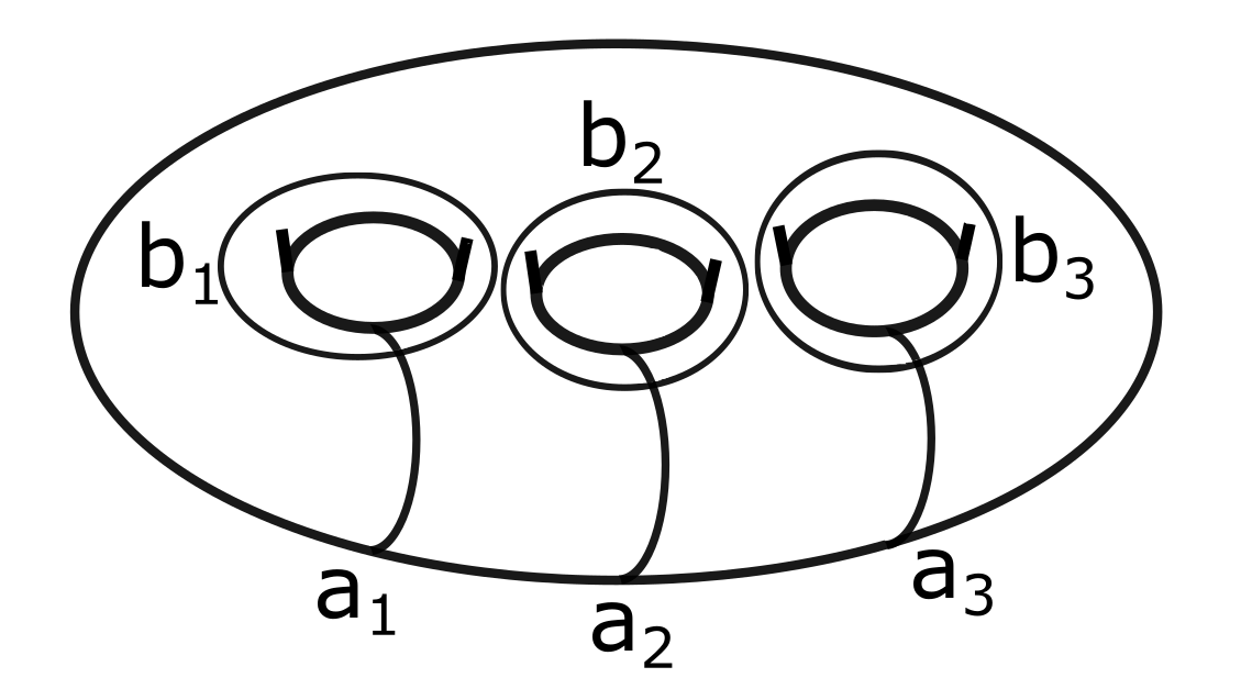
Figure 13.

In the setting of tangle diagrams given in Section $3$, if we start from Figure 2 we find that our model for $S^{3}$ is given by Figure 14. We know from Johnson that the Torelli group $\mathcal{I}_{g,1}$ is generated by bounding pair maps [Joh83a]. Here a bounding pair $d_{1},d_{2}$ is a pair of simple closed curves on the surface which bound a nontrivial subsurface, and the bounding pair map is given by $t_{d_{1}}t_{d_{2}}^{-1}$.

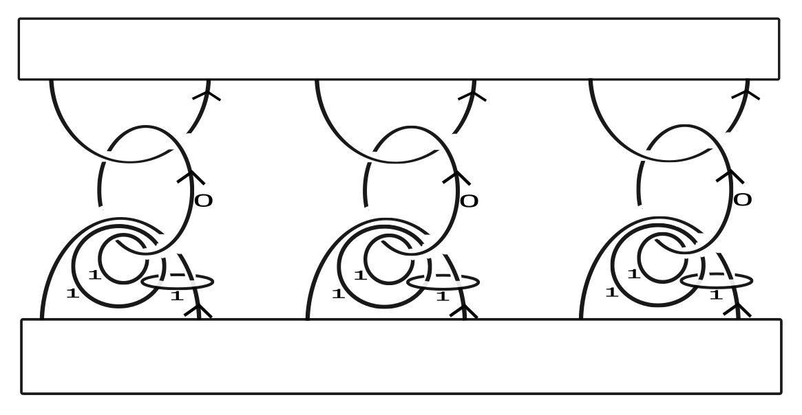
Figure 14.

From now on we suppose that $k\in\mathcal{I}_{g,1}$ is given as a product of bounding pair maps. We wish to use tangle diagrams and the method of composing tangles as in Lemma 3.1 to compute $\mu(V(k))$. To do this we will start by using simpler notation for the tangle diagrams we use, which is defined using Figure 15.

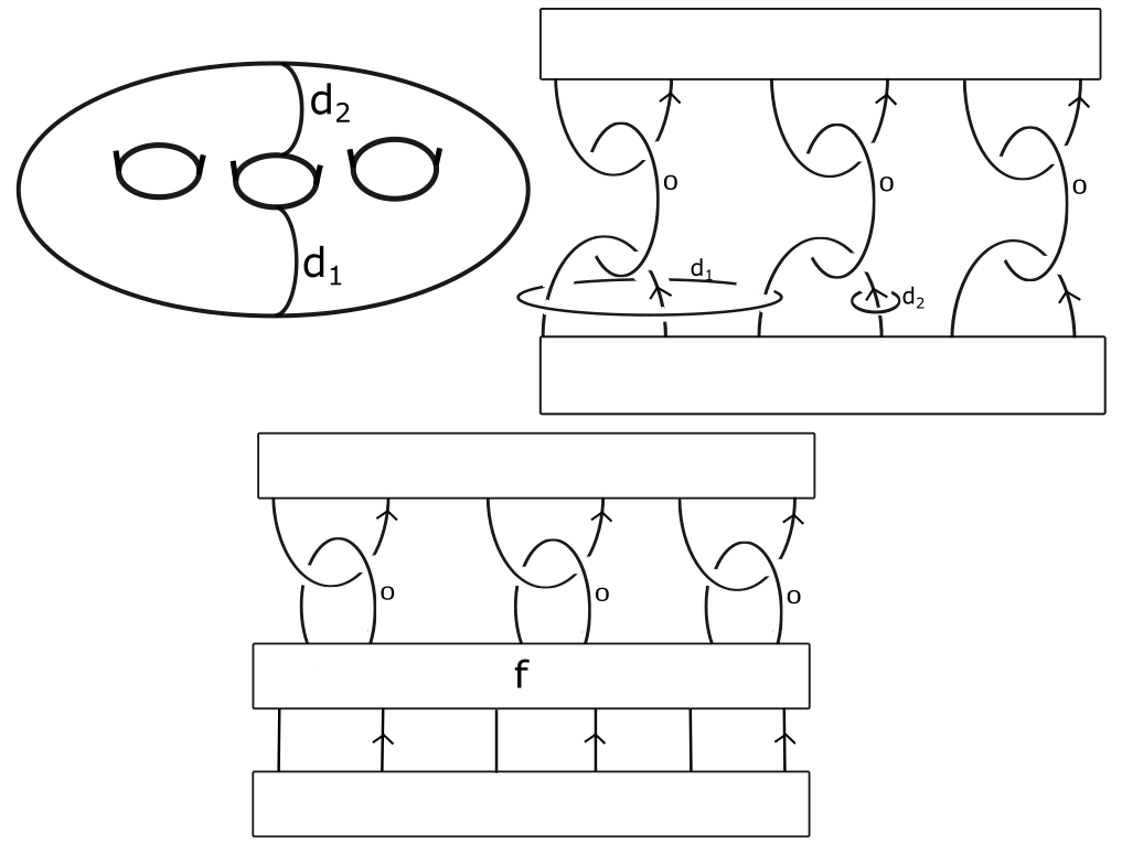
Figure 15. Simplified notation for a tangle diagram of $S(f)$ where $f=t_{d_{1}}t_{d_{2}}^{-1}$, where the framing of $d_{1},d_{2}$ giving the correct gluing has been suppressed.

Our notation works for concatenating tangle diagrams and will allow us to give a proof that the map $\mu:\mathcal{I}_{g,1}\rightarrow\mathbb{Z}/2$ given by sending $k\in\mathcal{I}_{g,1}$ to $\mu(V(k))$ is a homomorphism. Note that all our models for $V(k)$ give homology spheres which implies that the spin structure is unique. This implies that the characteristic sublink of the closed components of the tangle diagram is unique once we give orientations. We begin by showing that the characteristic sublink has a strightforward description in terms of the tangle diagrams. This description leads to a proof that the maps are homomorphisms and will be illustrated by an example.

First note that a sublink $C$ of a framed link $L$ is characteristic if $C\cdot L_{i}=L_{i}\cdot L_{i}\pmod{2}$. If we define the matrix of the linking form to be $A=(a_{ij})$ where

$$a_{ij}=\left\{\begin{array}[]{ll}lk(L_{i},L_{j}),&i\neq j\\ fr(L_{i}),&i=j\end{array}\right.$$

then the characteristic sublink condition becomes

(10) $$\sum_{L_{i}\in C}a_{ij}=a_{jj}\pmod{2},$$

for all $j$. We have that $V(k)$ has a unique characteristic sublink when written by a framed link and we will use (10) to find this sublink. The proof that the map $\mu$ is a homomorphism is by induction on the length of a word in bounding pair maps. The inductive step will be illustrated by the example given by Figure 16. We are now ready to give our new proof.

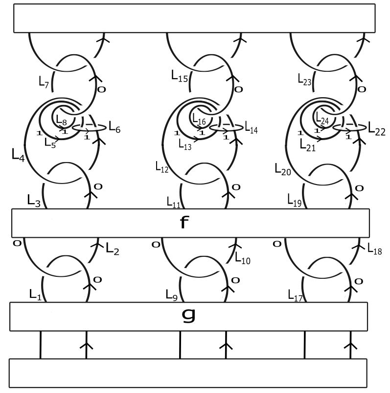
Figure 16. Simplified notation for a tangle diagram of $V(f\circ g)$ obtained by concatenation.

Theorem 5.1.

[BC78, Theorem 8] The map $\mu:\mathcal{I}_{g,1}\rightarrow\mathbb{Z}/2$ given above is a homomorphism.

Proof.

We illustrate the proof by using Figure 16 with $f=t_{d_{1}}t_{e_{1}}^{-1}$ and $g=t_{d_{2}}t_{e_{2}}^{-1}$ bounding pair maps. Let $\lambda$ denote the Seifert linking form for the standard embedding $h:\Sigma_{g}\rightarrow S^{3}$ given above.

The linking matrix for the closed components in the tangle diagram can be written as

$$R=\begin{bmatrix}B&\dots&\dots&0&0&A_{1}&D_{1}\\ 0&\ddots&\dots&\dots&0&A_{2}&D_{2}\\ 0&\dots&\ddots&\dots&0&\vdots&\vdots\\ 0&0&\dots&\ddots&0&\vdots&\vdots\\ 0&\dots&\dots&\dots&B&A_{n}&D_{n}\\ A_{1}^{\prime}&A_{2}^{\prime}&\dots&\dots&A_{n}^{\prime}&A&0\\ D_{1}^{\prime}&D_{2}^{\prime}&\dots&\dots&D_{n}^{\prime}&0&D\\ \end{bmatrix}.$$

Here $B$ is the linking matrix of the components $(L_{i})_{i=1}^{8}$, $(L_{i})_{i=9}^{16}$ and $(L_{i})_{i=17}^{24}$ from Figure 16 and the columns and rows coming from the $2\times 2$ matrices $A$ and $D$ come from the bounding pairs $d_{i}\cup e_{i}$. In general if our mapping class is a product of $n$ bounding pairs, the linking matrix $B$ is a $(2n+4)\times(2n+4)$ matrix with signature $2$, and there are $g$ copies of the matrix $B$ along the diagonal.

Since the $d_{i}\cup e_{i}$ are bounding pairs, they have the same linking number with the components $L_{i}$ up to signs. As they come in pairs the condition (10) for the characteristic sublink $C$ implies that they have no effect on whether $L_{i}\in C$ for $i=1,..,24$ and that the $d_{i}\cup e_{i}$ are either both in or both out of $C$. If we calculate using (10) we get that $L_{5}\cup L_{8}\cup L_{13}\cup L_{16}\cup L_{21}\cup L_{24}\in C$ always and $L_{i}\notin C$ for $i\neq 5,8,13,16,21,24,1\leq i\leq 24$. This pattern holds for any such framed link description of $V(k)$ obtained from tangle diagrams as above, and it is independent of the genus $g$ and the product of bounding pairs we start with. We also compute that $d_{i}\cup e_{i}\in C$ if $\lambda(d_{i},d_{i})$ is even and $d_{i}\cup e_{i}\notin C$ if $\lambda(d_{i},d_{i})$ is odd. Hence additivity of the $8\operatorname{\mathrm{Arf}}(C)$ terms in formula (9) follows because the $d_{i}\cup e_{i}$ are disjoint from each other.

To complete the proof we will show that if we orient each bounding pair $d_{i}\cup e_{i}$ oppositely then the $\Lambda_{L}-C\cdot C$ terms in formula (9) is always zero. To deal with the signature term of formula (9) for our chosen tangle diagrams, we use Sylvester’s law of inertia. Suppose we orient the $d_{i}\cup e_{i}$ so that the linking numbers have opposite signs. If the matrix $A$ corresponds to the bounding pair $d_{i}\cup e_{i}$ then $A$ has the form

$$\begin{bmatrix}\lambda(d_{i},d_{i})+1&-\lambda(d_{i},d_{i})\\ -\lambda(d_{i},d_{i})&\lambda(d_{i},d_{i})-1\end{bmatrix},$$

the matrices $A_{i}$ have identical columns but with opposite signs and the $A_{i}^{\prime}$ have identical rows but with opposite signs. Recall that if $E$ is an elementary matrix for a row operation then the matrix $ERE^{T}$ is obtained from the matrix $R$ by a simultaneous row and column operation. Then Sylvester’s law of inertia tells us that the signatures of $R$ and $ERE^{T}$ are equal. We can then repeatedly apply these operations to get a matrix of the form

$$R^{\prime}=\begin{bmatrix}B&\dots&\dots&0&0&0&0\\ 0&\ddots&\dots&\dots&0&0&0\\ 0&\dots&\ddots&\dots&0&\vdots&\vdots\\ 0&0&\dots&\ddots&0&\vdots&\vdots\\ 0&\dots&\dots&\dots&B&0&0\\ 0&0&\dots&\dots&0&A^{\prime}&0\\ 0&0&\dots&\dots&0&0&D^{\prime}\\ \end{bmatrix}.$$

Here the signature of the matrices $A^{\prime}$ and $D^{\prime}$ is the same as the signature of the matrices $A$ and $D$ respectively. Since the signature of any matrix of the form

$$\begin{bmatrix}m+1&-m\\ -m&m-1\end{bmatrix}$$

is zero, we get that

$$\Lambda_{L}-C\cdot C=2g-2g=0.$$

∎

As an aside we note that the signature calculation given in the previous proof along with the proof of Lemma 4.3 imply that the assignment $\mu_{\sigma}:\operatorname{\mathrm{Mod}}_{g,1}[2]\rightarrow\mathbb{Z}/8$ given by $\mu(f)=R(M_{f},\theta(\sigma))$ is also a homomorphism.

5.2. Evaluation on separating twists

The aim of the rest of this section is to refine formulas for evaluating Sato’s maps on elements of the Torelli group such as separating twists and bounding pair maps. The homological conditions that define separating curves and bounding pairs will be translated into statements about linking numbers in tangle diagrams. In some cases we will then be able to relate Sato’s maps to the Birman–Craggs maps.

We will need the following evaluation of $\mu(h,-)$ where $h$ is the inclusion, so we think of the Heegaard surface as being in $S^{3}$ [Joh80, Theorem 1].

Theorem 5.2.

Let $\gamma$ be a separating simple closed curve on the Heegaard surface, then

$$\mu(h,t_{\gamma})=\operatorname{\mathrm{Arf}}(\gamma).$$

Here $\operatorname{\mathrm{Arf}}(\gamma)$ can be evaluated by taking the subsurface $S\subset\Sigma_{g}$ which $\gamma$ bounds and calculating the Arf invariant of the quadratic form induced by the Seifert pairing on the Heegaard surface.

We can now begin relating Sato’s maps to the Birman–Craggs maps.

Corollary 5.3.

Let $\gamma$ be a separating simple closed curve in $\Sigma_{g}$, then

$$\beta_{\sigma,x}(t_{\gamma})=4(\operatorname{\mathrm{Arf}}(\theta(\sigma))-\operatorname{\mathrm{Arf}}(\theta(\sigma+x))).$$

Proof.

Since $\gamma$ is a separating simple closed curve we have that $\gamma=0\in H_{1}(\Sigma_{g};\mathbb{Z})$. For a fiber surface as pictured in Figure 2, the components coming from this diagram can all be isotoped in $S^{3}$ onto the canonical basis for $H_{1}(\Sigma_{g};\mathbb{Z})$ in the fiber. This means that the linking number of $\gamma$ with these components is the same as taking the algebraic intersection of $\gamma$ with the corresponding basis vector. Since $\gamma$ is separating this implies that $\gamma$ has linking number $0$ with all these components. This implies that the linking matrix of $L$ described by the methods of Section $3$, with $M_{L}\cong M_{t_{\gamma}}$, is zero everywhere except for one entry on the main diagonal, which is the framing of the curve $\gamma$. We compute that this framing is given by $\lambda(\gamma,\gamma)-1=\lambda(0,0)-1=-1$

For any spin structure $\sigma\in\operatorname{\mathrm{Spin}}(\Sigma)$, using the relators of Proposition 4.1 we have that

$$\theta(\sigma)(-1\mu)+0=1\pmod{2},$$

where $\mu$ is the meridian of the link component coming from $\gamma$ (and we abuse notation for the maps defined in Section $4.1$). Using our description of $\theta$, this implies that the link component corresponding to $\gamma$ is always in the characteristic sublink. This gives us that $\theta(\sigma+x)\cdot\theta(\sigma+x)-\theta(\sigma)\cdot\theta(\sigma)=0$ always, so we have that

$$\beta_{\sigma,x}(t_{\gamma})=4(\operatorname{\mathrm{Arf}}(\theta(\sigma))-\operatorname{\mathrm{Arf}}(\theta(\sigma+x))).$$

∎

Note that as a consequence of the proof just given we have the following relation between the Rochlin invariant and the Arf invariant:

$$R(M_{t_{\gamma}},\theta(\sigma))=8\operatorname{\mathrm{Arf}}(\theta(\sigma))\pmod{16},$$

when $\gamma$ is separating.

Next, we note that for $g\in\operatorname{\mathrm{Mod}}_{g,1}[2]$ and $f\in\operatorname{\mathrm{Mod}}_{g,1}$ we have that the diffeomorphism $f^{-1}\times id$ descends to a diffeomorphism $M_{fgf^{-1}}\rightarrow M_{g}$ of mapping tori. Under this diffeomorphism the spin structure $\theta(\sigma)$ on $M_{fgf^{-1}}$ is sent to the spin structure $\theta(f^{*}\sigma)$ on $M_{g}$. This implies that

$$R(M_{fgf^{-1}},\theta(\sigma))=R(M_{g},\theta(f^{*}\sigma)),$$

for all $f\in\operatorname{\mathrm{Mod}}_{g,1}$ and $g\in\operatorname{\mathrm{Mod}}_{g,1}[2]$.

If we set $\theta(\sigma)$ to contain none of the components coming from the chosen diagram for $\Sigma_{g}\times S^{1}$ we get that

$$R(M_{t_{\gamma}},\theta(\sigma))=8\operatorname{\mathrm{Arf}}(\gamma)\pmod{16}$$

which can be computed using the cut surface of $\gamma\subset\Sigma_{g,1}$ and the quadratic form on $H_{1}(\Sigma_{g})$ induced by the Seifert pairing on $\Sigma_{g,1}\subset S^{3}$. Johnson proved that $\operatorname{\mathrm{Spin}}(\Sigma_{g})$ is in bijective correspondence with quadratic forms induced by the intersection from on $H_{1}(\Sigma_{g})$ (see [Joh80a]). It is one of Arf’s theorems that two symplectic quadratic forms are in the same Sp-orbit if and only if they have the same Arf invariant. This implies that there are exactly two $\operatorname{\mathrm{Mod}}_{g,1}$ orbits of $\operatorname{\mathrm{Spin}}(\Sigma_{g})$. Suppose we picked an $x\in H^{1}(\Sigma_{g})$ such that $\sigma+x\in\operatorname{\mathrm{Spin}}(\Sigma_{g})$ is in the same orbit as $\sigma$, then we can write $\sigma+x=f^{*}\sigma$ for some $f\in\operatorname{\mathrm{Mod}}_{g,1}$ and we have that

$$\beta_{\sigma,x}(t_{\gamma})=(R(M_{t_{\gamma}},\theta(\sigma))-R(M_{t_{\gamma}},\theta(f^{*}\sigma)))/2=(R(M_{t_{\gamma}},\theta(\sigma))-R(M_{ft_{\gamma}f^{-1}},\theta(\sigma)))/2,$$

where $ft_{\gamma}f^{-1}=t_{f(\gamma)}$ and $f(\gamma)$ is also a separating curve of the same genus, on the fiber surface. So we have that

$$\beta_{\sigma,x}(t_{\gamma})=4(\operatorname{\mathrm{Arf}}(\gamma)-\operatorname{\mathrm{Arf}}(f(\gamma)))\pmod{8}.$$

Note that surgery along $\gamma\subset\Sigma_{g,1}$ with framing $-1$ is equivalent to cutting $S^{3}$ open along a Heegaard surface and regluing by $t_{\gamma}$, since $t_{\gamma}$ acts trivially on homology this gives a homology sphere. So the formulas given above relate the Rochlin invariant of mapping tori to the Rochlin invariant of homology spheres and Johnson’s description of the Birman-Craggs homomorphisms [Joh80]. In summary, if we combine Theorem 5.2 and Corollary 5.3 with the discussion above we get the following.

Corollary 2.

If we have that $\sigma=f^{*}(\eta)$ and $\sigma+x=g^{*}(\eta)$ for $f,g\in\operatorname{\mathrm{Mod}}_{g,1}$ with $\eta$ the spin structure giving minimal number of components for the characteristic sublink $\theta(\eta)$, then

$$\beta_{\sigma,x}(t_{c})=\mu(t_{f(c)})-\mu(t_{g(c)})\pmod{2},$$

where $\mu$ denotes the Birman-Craggs homomorphism for the standard embedding $\Sigma_{g}\hookrightarrow S^{3}$.

5.3. Evaluation on bounding pairs

By definition, a bounding pair is a pair of disjoint, homologous, non-separating simple closed curves on $\Sigma_{g}$ and the bounding pair map is $t_{a}t_{b}^{-1}$. Firstly we place the bounding pair $a,b$ in a fiber in the Kirby diagram. A similar argument to the previous section implies that for any component $L_{i}$ we have that $lk(L_{i},a)=lk(L_{i},b)$. Suppose we have that $\lambda(a,a)=\lambda(b,b)=\lambda(a,b)=lk(a,b)=m$, we will inspect the linking matrix terms in the formula

$$\beta_{\sigma,x}([\varphi])=(\theta(\sigma+x)\cdot\theta(\sigma+x)-\theta(\sigma)\cdot\theta(\sigma)+8(\operatorname{\mathrm{Arf}}(\theta(\sigma))-\operatorname{\mathrm{Arf}}(\theta(\sigma+x))))/2\pmod{8}.$$

Write $L_{a},L_{b}$ for the components coming from the bounding pair, with meridians $\mu_{a},\mu_{b}$ respectively. Using Proposition 4.1 we must have that

$$w((m+1)\mu_{a}+\sum_{j\neq a,b}lk(L_{a},L_{j})\mu_{j}+m\mu_{b})=w((m-1)\mu_{b}+\sum_{j\neq b,a}lk(L_{b},L_{j})\mu_{j}+m\mu_{a})=m+1\pmod{2},$$

which simplifies to

(11) $$w((m+1)\mu_{a}+m\mu_{b})=w((m-1)\mu_{b}+m\mu_{a})=m+1-\sum_{j\neq a,b}lk(L_{a},L_{j})w(\mu_{j})\pmod{2}.$$

From this we see that $L_{a}$ and $L_{b}$ are always either both in, or both out of any characteristic sublink of $L$. Now reverse the orientation on the component $L_{b}$, this does not change the framing of $L_{b}$ but changes the sign of the linking number of $L_{b}$ with every other component, the characteristic sublink is also the same as before. This means that up to the ordering of the indices for the components of the link, we have the following linking matrix for the surgery diagram for $M_{L}\cong M_{t_{a}t_{b}^{-1}}$ obtained from our ribbon graph for $\#_{g}S^{1}\times S^{2}$

$$\begin{bmatrix}0&\dots&\dots&0&0&0\\ 0&\dots&\dots&0&a_{1}&-a_{1}\\ 0&\dots&\dots&0&a_{2}&-a_{2}\\ 0&\ddots&\dots&0&\vdots&\vdots\\ 0&\dots&\dots&0&a_{2g}&-a_{2g}\\ 0&a_{1}&\dots&a_{2g}&m+1&-m\\ 0&-a_{1}&\dots&-a_{2g}&-m&m-1\\ \end{bmatrix}.$$

Suppose we have that $L_{a}\cup L_{b}\in\theta(\sigma)$, then since $\theta(\sigma)\cdot\theta(\sigma)$ is the sum of the entries in the linking matrix of the characteristic sublink $\theta(\sigma)$ we have that

$$\theta(\sigma)\cdot\theta(\sigma)=m+1+m-1-2m=0,$$

similarly if $L_{a}\cup L_{b}\notin\theta(\sigma)$ then $\theta(\sigma)\cdot\theta(\sigma)=0$. By the discussion above these are all the cases and so we have that

$$\beta_{\sigma,x}(t_{a}t_{b}^{-1})=4(\operatorname{\mathrm{Arf}}(\theta(\sigma))-\operatorname{\mathrm{Arf}}(\theta(\sigma+x)))\pmod{8}.$$

Since the Torelli group is generated by bounding pair maps this describes the homomorphisms $\beta_{\sigma,x}$ on the Torelli group fully.

From now on let $\eta\in\operatorname{\mathrm{Spin}}(\Sigma_{g})$ denote the spin structure with the characteristic sublink of $\theta(\eta)$ containing none of the components coming from the chosen diagram for $\Sigma_{g}\times S^{1}$. If we use the relations of (11) we have that if $m=lk(a,b)$ is even then

$$w(\mu_{a})=w(\mu_{b})=1\pmod{2},$$

so $L_{a}\cup L_{b}\in\theta(\eta)$ and we have that

$$R(M_{t_{a}t_{b}^{-1}},\theta(\eta))=\Lambda_{L}+8\operatorname{\mathrm{Arf}}(a\cup b)=8\operatorname{\mathrm{Arf}}(a\cup b),$$

where $\Lambda_{L}$ is the signature of the linking matrix given above. Here $\operatorname{\mathrm{Arf}}(a\cup b)$ can be computed using the cut surface of $a\cup b\subset\Sigma_{g,1}$ and the quadratic form induced by the Seifert pairing of $\Sigma_{g,1}\subset S^{3}$.

If $m$ is odd then we compute that

$$m\omega(\mu_{b})=0\pmod{2},$$

so $L_{a}\cup L_{b}\notin\theta(\eta)$ and we have that

$$R(M_{t_{a}t_{b}^{-1}},\theta(\eta))=\Lambda_{L}=0.$$

Notice that for $a\cup b\subset\Sigma_{g,1}$, surgery with coefficients $m\pm 1$ is equivalent to cutting $S^{3}$ open along a Heegaard surface and regluing by $t_{a}t_{b}^{-1}$. Since $t_{a}t_{b}^{-1}$ acts trivially on homology the resulting space is a homology sphere. So we have found a relation between the Rochlin invariants of a mapping tori and a homology spheres.

Now we relate Sato’s maps on bounding pairs to the Birman–Craggs maps using the same method as in the case of separating curves. Suppose we have a spin structure $\sigma\in\operatorname{\mathrm{Spin}}(\Sigma_{g})$ and a class $x\in H^{1}(\Sigma_{g})$ such that there exists mapping classes $f,g\in\operatorname{\mathrm{Mod}}_{g,1}$ with $\sigma=f^{*}(\eta)$ and $\sigma+x=g^{*}(\eta)$. We have

$$\beta_{\sigma,x}(t_{a}t_{b}^{-1})=(R(M_{t_{a}t_{b}^{-1}},\theta(f^{*}(\eta)))-R(M_{t_{a}t_{b}^{-1}},\theta(g^{*}(\eta))))/2\\ =(R(M_{t_{f(a)}t_{f(b)}^{-1}},\theta(\eta)))-R(M_{t_{g(a)}t_{g(b)}^{-1}},\theta(\eta)))/2.$$

We will also need the following calculation of the Birman–Craggs maps, due to Johnson. Note that this calculation will also follow from the proof of Theorem 5.1.

Lemma 5.4.

[Joh80, Theorem 1] Let $a,b$ be a pair of simple closed curves on $\Sigma_{g,1}$ that bound a subsurface, and let $\lambda:H_{1}(\Sigma_{g};\mathbb{Z})\times H_{1}(\Sigma_{g};\mathbb{Z})\rightarrow\mathbb{Z}$ denote the Seifert linking form for the standard embedding $\Sigma_{g}\hookrightarrow S^{3}$. Then for the Birman-Craggs map $\mu:\mathcal{I}_{g,1}\rightarrow\mathbb{Z}/2$ corresponding to the embedding $\Sigma_{g}\hookrightarrow S^{3}$ we have that:

1. $\mu(t_{a}t_{b}^{-1})=0$ if $\lambda(a,a)$ is odd,

2. $\mu(t_{a}t_{b}^{-1})=8\operatorname{\mathrm{Arf}}(a\cup b)$ if $\lambda(a,a)$ is even.

In summary if we combine Lemma 5.4 with the calculations of this subsection we have the following result.

Corollary 3.

Let $a,b$ be a pair of simple closed curves on $\Sigma_{g,1}$ that bound a subsurface. If we have that $\sigma=f^{*}(\eta)$ and $\sigma+x=g^{*}(\eta)$ for $f,g\in\operatorname{\mathrm{Mod}}_{g,1}$ with $\eta$ the spin structure giving the minimal number of components for the characteristic sublink $\theta(\eta)$, then

$$\beta_{\sigma,x}(t_{a}t_{b}^{-1})=\mu(t_{f(a)}t_{f(b)}^{-1})-\mu(t_{g(a)}t_{g(b)}^{-1}),$$

where $\mu$ denotes the Birman–Craggs homomorphism for the standard embedding $\Sigma_{g}\hookrightarrow S^{3}$.

6. The abelianization of $\operatorname{\mathrm{Mod}}_{g,1}[2]$

In this section we give an alternative description of $H_{1}(\operatorname{\mathrm{Mod}}_{g,1}[2];\mathbb{Z})$ by defining a family of polynomial algebras indexed by a spin structure $\sigma\in\operatorname{\mathrm{Spin}}(\Sigma_{g})$. We rewrite Sato’s homomorphisms as maps from $\operatorname{\mathrm{Mod}}_{g,1}[2]$ to this algebra. We can then use a single relation in this polynomial algebra repeatedly to calculate the image of Sato’s maps on certain subgroups. Let us begin by recalling some of the results in Sato’s paper [Sat10].

We have the following function $i_{z}:H_{1}(\Sigma_{g})\rightarrow\mathbb{Z}/8$ ($H_{1}(\Sigma_{g})$ always assumed with $\mathbb{Z}/2$ coefficients unless specified otherwise)

$$i_{z}(y)=\left\{\begin{array}[]{ll}1,&z\cdot y=1\mod 2\\ 0,&z\cdot y=0\mod 2\end{array}\right.$$

This function is not a homomorphism but we have the following two identities

(12) $$i_{a}(x)+i_{b}(x)-2i_{a}(x)i_{b}(x)=i_{a+b}(x),$$

(13) $$((-1)^{q_{\sigma}(C)}i_{C}(x))^{2}=(-1)^{q_{\sigma}(C)}((-1)^{q_{\sigma}(C)}i_{C}(x))$$

where $q_{\sigma}$ is a quadratic form. Both identities are checked by comparing both sides of the equation elementwise.

We will need to make use of the following results of Sato.

Corollary 6.1.

[Sat10, Lemma 2.2, Propositions 5.2 and 7.1] Fix a spin structure $\sigma\in Spin(\Sigma_{g})$ and let $q_{\sigma}$ be the associated quadratic form on $H_{1}(\Sigma_{g})$. The map $\beta_{\sigma}:\operatorname{\mathrm{Mod}}_{g,1}[2]\rightarrow\operatorname{\mathrm{Map}}(H_{1}(\Sigma_{g}),\mathbb{Z}/8)$ given by $\beta_{\sigma}(t_{C}^{2})=(-1)^{q_{\sigma}(C)}i_{[C]}$ is a homomorphism and $|H_{1}(\operatorname{\mathrm{Mod}}_{g,1}[2];\mathbb{Z})|\leq|\mathbb{Z}/8^{2g}\bigoplus\mathbb{Z}/4^{2g\choose 2}\bigoplus\mathbb{Z}/2^{2g\choose 3}|$.

Note that $\operatorname{\mathrm{Map}}(H_{1}(\Sigma_{g}),\mathbb{Z}/8)$ is thought of as a $\mathbb{Z}/8$-module under function addition and scaling. If we add the operation function multiplication, this turns $\operatorname{\mathrm{Map}}(H_{1}(\Sigma_{g}),\mathbb{Z}/8)$ into a $\mathbb{Z}/8$-algebra. Using the identity given by (12), motivated by the formula of Corollary 6.1, we compute that

(14) $$(-1)^{q_{\sigma}(C_{1}+C_{2})}i_{C_{1}+C_{2}}(x)=(-1)^{q_{\sigma}(C_{1}+C_{2})}(i_{C_{1}}(x)+i_{C_{2}}(x)-2i_{C_{1}}(x)i_{C_{2}}(x))\\ =(-1)^{q_{\sigma}(C_{2})+C_{1}\cdot C_{2}}((-1)^{q_{\sigma}(C_{1})}i_{C_{1}}(x))+(-1)^{q_{\sigma}(C_{1})+C_{1}\cdot C_{2}}((-1)^{q_{\sigma}(C_{2})}i_{C_{2}}(x))\\ -2(-1)^{q_{\sigma}(C_{1}+C_{2})}i_{C_{1}}(x)i_{C_{2}}(x).$$

We also have that

(15) $$(-1)^{q_{\sigma}(C_{1})}i_{C_{1}}(x)(-1)^{q_{\sigma}(C_{2})}i_{C_{2}}(x)=(-1)^{q_{\sigma}(C_{1}+C_{2})-C_{1}\cdot C_{2}}i_{C_{1}}(x)i_{C_{2}}(x),$$

if we set $\overline{C}=(-1)^{q_{\sigma}(C)}i_{C}$ and plug (15) into the last line of (14), we get that,

(16) $$\overline{C_{1}+C_{2}}=(-1)^{q_{\sigma}(C_{2})+C_{1}\cdot C_{2}}\overline{C_{1}}+(-1)^{q_{\sigma}(C_{1})+C_{1}\cdot C_{2}}\overline{C_{2}}-2(-1)^{C_{1}\cdot C_{2}}\overline{C_{1}}\overline{C_{2}}\\ =(-1)^{C_{1}\cdot C_{2}}((-1)^{q_{\sigma}(C_{2})}\overline{C_{1}}+(-1)^{q_{\sigma}(C_{1})}\overline{C_{2}}-2\overline{C_{1}}\overline{C_{2}}).$$

We summarise equations (13) and (16) by the following two relations between the $\overline{C_{i}}$’s as functions.

Let $\sigma\in Spin(\Sigma_{g})$ and denote by $q_{\sigma}$ the associated quadratic form. Then in the subalgebra $Z_{\sigma}$ of $\operatorname{\mathrm{Map}}(H_{1}(\Sigma_{g}),\mathbb{Z}/8)$ generated by $\overline{C}$ for all $C\in H_{1}(\Sigma_{g})$, the following relations hold:

(17) $$\overline{C_{1}+C_{2}}=(-1)^{C_{1}\cdot C_{2}}((-1)^{q_{\sigma}(C_{2})}\overline{C_{1}}+(-1)^{q_{\sigma}(C_{1})}\overline{C_{2}}-2\overline{C_{1}}\overline{C_{2}}),$$

for all $C_{1}\neq C_{2}\in H_{1}(\Sigma_{g})$.

(18) $$\overline{C}^{2}=(-1)^{q_{\sigma}(C)}\overline{C},$$

for all $C\in H_{1}(\Sigma_{g})$.

Fix a symplectic basis $B=\{A_{1},B_{1},....,A_{g},B_{g}\}$ for $H_{1}(\Sigma_{g})$ with $A_{i}\cdot B_{j}=\delta_{ij}$, $A_{i}\cdot A_{j}=0$ and $B_{i}\cdot B_{j}=0$.

Since we have that any $C\in H_{1}(\Sigma_{g})$ can be written uniquely as a linear combination of the $A_{i},B_{i}$’s so iteratively applying the defining relations (17) and (18) of $Z_{\sigma}$ implies that any element in the $\mathbb{Z}/8$-submodule $\operatorname{\mathrm{im}}{\beta_{\sigma}}$ spanned by the $\overline{C_{i}}$’s can be written as a linear combination of elements of the form

(19) $$\overline{X_{i}},2\overline{X_{i}}\overline{X_{j}},4\overline{X_{i}}\overline{X_{j}}\overline{X_{k}},$$

where $X_{i},X_{j}$ and $X_{k}$ are distinct elements from $B$. We wish to prove that

$$\operatorname{\mathrm{im}}{\beta_{\sigma}}=\mathbb{Z}/8^{2g}\bigoplus 2\mathbb{Z}/8^{2g\choose 2}\bigoplus 4\mathbb{Z}/8^{2g\choose 3}$$

as a submodule, this will follow from the following result.

Proposition 6.2.

If a $\mathbb{Z}/8$-linear combination of elements of the form (19) is equal to zero, then the coefficients of the monomial terms must be $0$ and the coefficients of the $2\overline{X_{i}}\overline{X_{j}},4\overline{X_{i}}\overline{X_{j}}\overline{X_{k}}$ terms must be either $0$ or zero divisors.

Proof.

Suppose that we had such a linear combination $f\in\operatorname{\mathrm{Map}}(H_{1}(\Sigma_{g}),\mathbb{Z}/8)$ that was equal to the constant zero function. Since $B$ is a symplectic basis, the definition of the functions $i_{[C]}$ gives us the following.

(i) If $X_{i}\in B$ then $i_{X_{i}}(X_{j})=1$ for the unique $X_{j}\in B$ with $X_{i}\cdot X_{j}=\pm 1$, and it is $0$ on every other element of $B$. This implies that for distinct $X_{i},X_{j},X_{k}$ in $B$ we have that $i_{X_{i}}(X_{l})i_{X_{j}}(X_{l})=i_{X_{i}}(X_{l})i_{X_{j}}(X_{l})i_{X_{k}}(X_{l})=0$ for any $X_{l}\in B$.

Using (i), if we evaluate $f$ on all elements of $B$ we must have that all the monomial coefficients are zero as $\overline{C}(X_{i})$ can only take values $0,\pm 1$. So we must have that $f$ has no monomial terms.

(ii) Similarly we have that if $X_{i},X_{j},X_{k},X_{l}\in B$ with $X_{i},X_{j}$ distinct, then $i_{X_{i}}(X_{l}+X_{k})i_{X_{j}}(X_{l}+X_{k})$ can only be nonzero if up to reordering indices we have that $X_{i}\cdot X_{l}=\pm 1$ and $X_{j}\cdot X_{k}=\pm 1$. Since $B$ is a symplectic basis this tuple $(X_{l},X_{k})$ is unique and from this we get that for $X_{i},X_{j},X_{k}\in B$ distinct we have that $i_{X_{i}}(X_{l}+X_{n})i_{X_{j}}(X_{l}+X_{n})i_{X_{k}}(X_{l}+X_{n})$ is zero for all $X_{l},X_{n}\in B$ and $i_{X_{i}}(X_{l}+X_{k})i_{X_{j}}(X_{l}+X_{k})$ is only non-zero for one element $X_{r}+X_{s}$.

Using (ii), if we then evaluate $f$ on all elements of the form $X_{l}+X_{n}$ we get that all the coefficients of the quadratic terms of $f$ must be either $0$ or zero divisors, and so $f$ can only contain cubic terms.

(iii) If $X_{i},X_{j},X_{k}\in B$ are distinct then $i_{X_{i}}(X_{a}+X_{b}+X_{c})i_{X_{j}}(X_{a}+X_{b}+X_{c})i_{X_{k}}(X_{a}+X_{b}+X_{c})$ can only be nonzero if, up to reordering, we have that $X_{i}\cdot X_{a}=\pm 1$, $X_{j}\cdot X_{b}=\pm 1$, $X_{k}\cdot X_{c}=\pm 1$. Since $B$ is a symplectic basis, this sum is unique, so evaluating $f$ on all elements of the form $X_{a}+X_{b}+X_{c}$ gives the result. ∎

Combining this result with the last statement of Corollary 6.1 gives us that

$$H_{1}(\operatorname{\mathrm{Mod}}_{g,1}[2];\mathbb{Z})=\mathbb{Z}/8^{2g}\bigoplus 2\mathbb{Z}/8^{2g\choose 2}\bigoplus 4\mathbb{Z}/8^{2g\choose 3}.$$

We wish to simplify the description of the abelianization slightly to have a more compact form, to do this we define the following family of squarefree polynomial algebras $W_{\sigma}$ indexed by $\sigma\in Spin(\Sigma_{g})$.

Let $W_{\sigma}$ denote the unital associative commutative $\mathbb{Z}/8$-algebra generated by $\overline{C}$ for all $C\in H_{1}(\Sigma_{g})$, subject to the following relations:

(i) $\overline{C_{1}+C_{2}}=(-1)^{C_{1}\cdot C_{2}}((-1)^{q_{\sigma}(C_{2})}\overline{C_{1}}+(-1)^{q_{\sigma}(C_{1})}\overline{C_{2}}-2\overline{C_{1}}\overline{C_{2}}),$ for all $C_{1}\neq C_{2}\in H_{1}(\Sigma_{g})$.

(ii) $\overline{C}^{2}=(-1)^{q_{\sigma}(C)}\overline{C}$, for all $C\in H_{1}(\Sigma_{g})$.

We have the following.

Proposition 6.3.

The map $\Phi:W_{\sigma}\rightarrow\operatorname{\mathrm{Map}}(H_{1}(\Sigma_{g}),\mathbb{Z}/8)$ given by $\Phi(\overline{C})=(-1)^{q_{\sigma}(C)}i_{C}$ is an algebra homomorphism.

Proof.

Let $F$ denote the free $\mathbb{Z}/8$-algebra generated by all elements in $H_{1}(\Sigma_{g})$. We have the map $f:H_{1}(\Sigma_{g})\rightarrow\operatorname{\mathrm{Map}}(H_{1}(\Sigma_{g}),\mathbb{Z}/8)$ given by $f(C)=(-1)^{q_{\sigma}(C)}i_{C}$. The universal property for free algebras implies there exists a unique $\mathbb{Z}/8$-algebra homomorphism $\widetilde{\Phi}:F\rightarrow\operatorname{\mathrm{Map}}(H_{1}(\Sigma_{g}),\mathbb{Z}/8)$ extending $f$. Then the identities given by equations (16) and (13) imply that $\widetilde{\Phi}$ vanishes on the ideal $I$ generated by elements of the form

(i) $\overline{C_{1}+C_{2}}-(-1)^{C_{1}\cdot C_{2}}((-1)^{q_{\sigma}(C_{2})}\overline{C_{1}}+(-1)^{q_{\sigma}(C_{1})}\overline{C_{2}}-2\overline{C_{1}}\overline{C_{2}})$ for $C_{1}\neq C_{2}$, and

(ii) $\overline{C}^{2}-(-1)^{q_{\sigma}(C)}\overline{C}$ for all $C\in H_{1}(\Sigma_{g})$.

So $\widetilde{\Phi}$ descends to a homomorphism $W_{\sigma}\rightarrow\operatorname{\mathrm{Map}}(H_{1}(\Sigma_{g}),\mathbb{Z}/8)$, which is given by $\Phi$. This proves that $\Phi$ is a $\mathbb{Z}/8$-algebra homomorphism. ∎

From this and Proposition 6.2 we get that the map $\phi:\operatorname{\mathrm{im}}{\beta_{\sigma}}\rightarrow W_{\sigma}$ given by $\phi((-1)^{q_{\sigma}(C)}i_{C})=\overline{C}$ extends to a $\mathbb{Z}/8$-linear isomorphism onto the submodule of $W_{\sigma}$ generated by all the $\overline{C_{i}}$’s. Comparing values gives that $\phi$ is the inverse of $\Phi$ as a module map. This implies that the map

$$\phi\circ\beta_{\sigma}:\operatorname{\mathrm{Mod}}_{g,1}[2]\rightarrow W_{\sigma}$$

given by $\phi\circ\beta_{\sigma}(t_{C}^{2})=\overline{[C]}$ for $C$ non-separating and $[C]\in H_{1}(\Sigma_{g})$ its corresponding homology class, is a homomorphism. This map is also trivially $\operatorname{\mathrm{Mod}}_{g,1}$-equivariant if we make $\operatorname{\mathrm{Mod}}_{g,1}$ act on $W_{\sigma}$ via $f\overline{C}=\overline{f_{*}(C)}$. Now we can conveniently think of $\operatorname{\mathrm{im}}{\phi\circ\beta_{\sigma}}$ as the abelianization of $\operatorname{\mathrm{Mod}}_{g,1}[2]$.

6.1. Abelian quotients of the Torelli group

From now on we will write Sato’s homomorphisms using our description as maps $\phi\circ\beta_{\sigma}:\operatorname{\mathrm{Mod}}_{g,1}\rightarrow W_{\sigma}$. It has been previously computed in Section $5$ that these maps have image in a $\mathbb{Z}/2$-vector space when restricted to the Torelli group. Let us abuse notation and write $\beta_{\sigma}:\mathcal{I}_{g,1}\rightarrow W_{\sigma}$ for the family of homomorphisms obtained by restricting Sato’s homomorphisms $\phi\circ\beta_{\sigma}$ to the Torelli group. The aim of this subsection is to compute the image of the Torelli group under $\beta_{\sigma}$ in $W_{\sigma}$. To do this we will need a few results about bounding pair maps in the Torelli group.

Factorisation into squares

We can use the result under Proposition 4.12 of [FM11] to factor a genus $1$ bounding pair into a product of squares of Dehn twists. We define a chain of simple closed curves $c_{1},c_{2},c_{3}$ to be a triple such that $i(c_{1},c_{2})=i(c_{2},c_{3})=1$ and all other pairwise geometric intersection numbers are zero. Let $c_{1},c_{2},c_{3}$ be a chain of simple closed curves and let $d_{1},d_{2}$ be the boundary curves of a regular neighbourhood of $c_{1}\cup c_{2}\cup c_{3}$, then the chain relation gives that

$$(t_{c_{1}}^{2}t_{c_{2}}t_{c_{3}})^{3}=t_{d_{1}}t_{d_{2}}.$$

So we have that

$$(t_{c_{1}}^{2}t_{c_{2}}t_{c_{3}})^{3}=t_{c_{1}}^{2}(t_{c_{2}}t_{c_{3}}t_{c_{1}}^{2}t_{c_{3}}^{-1}t_{c_{2}}^{-1})(t_{c_{2}}t_{c_{3}})^{2}(t_{c_{1}}^{2}t_{c_{2}}t_{c_{3}})$$

$$=t_{c_{1}}^{2}(t_{c_{2}}t_{c_{3}}t_{c_{1}}^{2}t_{c_{3}}^{-1}t_{c_{2}}^{-1})(t_{c_{2}}t_{c_{3}})^{2}t_{c_{1}}^{2}(t_{c_{2}}t_{c_{3}})^{-2}(t_{c_{2}}t_{c_{3}})^{3}.$$

Using the braid relation we also have that the rightmost term in the last equality can be written as

$$(t_{c_{2}}t_{c_{3}})^{3}=t_{c_{3}}t_{c_{2}}t_{c_{3}}^{2}t_{c_{2}}t_{c_{3}}$$

$$=(t_{c_{3}}t_{c_{2}}t_{c_{3}}^{2}t_{c_{2}}^{-1}t_{c_{3}}^{-1})(t_{c_{3}}t_{c_{2}}^{2}t_{c_{3}})$$

$$=(t_{c_{3}}t_{c_{2}}t_{c_{3}}^{2}t_{c_{2}}^{-1}t_{c_{3}}^{-1})(t_{c_{3}}t_{c_{2}}^{2}t_{c_{3}}^{-1})t_{c_{3}}^{2},$$

and so we have the following factorisation

$$t_{d_{1}}t_{d_{2}}^{-1}=t_{c_{1}}^{2}t_{t_{c_{2}}t_{c_{3}}(c_{1})}^{2}t_{(t_{c_{2}}t_{c_{3}})^{2}(c_{1})}^{2}t_{t_{c_{3}}t_{c_{2}}(c_{3})}^{2}t_{t_{c_{3}}(c_{2})}^{2}t_{c_{3}}^{2}t_{d_{2}}^{-2}.$$

The images of the $\beta_{\sigma}$

To calculate the images of the Torelli group in the algebras $W_{\sigma}$, we use another result of Dennis Johnson[Joh83a]. The result we use is that these maps $t_{d_{1}}t_{d_{2}}^{-1}$ (running over all $d_{1},d_{2}$ bounding pairs of genus $1$) generate $\mathcal{I}_{g,1}$, so it will be enough to evaluate $\beta_{\sigma}$ on one such map and use Symplectic equivariance. Note that $\beta_{\sigma,x}(t_{c}^{2})$ only depends on the homology class $C$ of $c$ in $H_{1}(\Sigma_{g})$. From now on we will denote $C_{i}$ by the homology class of the curve $c_{i}$. Motivated by the formula for bounding pairs written above we compute that in $H_{1}(\Sigma_{g})$ we have that

$$t_{c_{2}}t_{c_{3}}(c_{1})=C_{1}+C_{2},$$

$$(t_{c_{2}}t_{c_{3}})^{2}(C_{1})=C_{1}+C_{2}+C_{3},$$

$$t_{c_{3}}t_{c_{2}}(C_{3})=C_{2},$$

$$t_{c_{3}}(C_{2})=C_{2}+C_{3}.$$

Note that $C_{1},C_{2},D_{1}=D_{2}$ can be completed into a symplectic basis for $H_{1}(\Sigma_{g})$. We will compute $\beta_{\sigma}(t_{d_{1}}t_{d_{2}}^{-1})$ in the language of the previous section by using relations (17) and (18). Plugging in the factorisation of a bounding pair we get that

$$\beta_{\sigma}(t_{d_{1}}t_{d_{2}}^{-1})=\overline{C_{1}}+\overline{C_{1}+C_{2}}+\overline{C_{1}+C_{2}+C_{3}}+\overline{C_{2}}+\overline{C_{2}+C_{3}}+\overline{C_{3}}-\overline{D_{1}}.$$

So $\operatorname{\mathrm{im}}{\beta_{\sigma}}$ is the submodule generated by $\{\overline{C_{1}}+\overline{C_{1}+C_{2}}+\overline{C_{1}+C_{2}+C_{3}}+\overline{C_{2}}+\overline{C_{2}+C_{3}}+\overline{C_{3}}-\overline{D_{1}}\}$ running over all chains $c_{1},c_{2},c_{3}$ of simple closed curves with $d_{1}\cup d_{2}=\partial(\nu(c_{1}\cup c_{2}\cup c_{3}))$. The computations of Section $5.4$ imply that this submodule is a $\mathbb{Z}/2$-vector space.

Let us choose a spin structure $\sigma$ with $q_{\sigma}(C_{1})=q_{\sigma}(C_{2})=q_{\sigma}(D_{1})=0$, then we have that $q_{\sigma}(C_{3})=q_{\sigma}(C_{1}+D_{1})=0$. For any such spin structure, the formula above simplifies and we get that

$$\beta_{\sigma}(t_{d_{1}}t_{d_{2}}^{-1})=4\overline{C_{1}}\overline{C_{2}}+4\overline{C_{1}}\overline{C_{2}}\overline{D_{1}}.$$

References

- [Akb77] S. Akbulut “On 2-dimensional homology classes of 4-manifolds” In Math. Proc. Camb. Phil. Soc., 82, 1977, pp. 99–106
- [BC78] J.. Birman and R. Craggs “The mu-invariant of manifolds and certain structural properties of the group of homemorphisms of a closed, oriented manifold” In Transactions of the American Mathematical Society, Volume 237, 1978, pp. 283–309
- [Far06] B. Farb “Problems on Mapping Class Groups and Related Topics” Proceedings of Symposia in Pure Mathematics Volume: 74, 2006
- [FFU01] Y. Fukumoto, M. Furuta and M. Ue “W-invariants and Neumann–Siebenmann invariants for Seifert homology 3-spheres” In Topology and its Applications 116, 2001, pp. 333–369
- [FM11] B. Farb and D. Margalit “A Primer on Mapping Class Groups” Princeton Mathematical Series - 49, 2011
- [GS99] R. Gompf and A. Stipsicz “4-manifolds and Kirby calculus” A.M.S. Graduate Studies in Mathematics, Volume: 20, 1999
- [Har82] J. Harer “How to construct all fibered knots and links” In Topology, Volume 21, No. 3, 1982, pp. 263–280
- [Hat02] A. Hatcher “Algebraic Topology” Cambridge University Press, 2002
- [Hos84] J. Hoste “The Arf Invariant of a Totally Proper Link” In Topology and its Applications 18, 1984, pp. 163–177
- [Hum92] S.. Humphries “Normal closures of powers of Dehn twists in mapping class groups.” In Glasgow Math. J. 34, 1992, pp. 313–317
- [Joh80] D. Johnson “Quadratic forms and the Birman-Craggs homomorphisms” In Transactions of the American Mathematical Society, Vol. 261, 1980, pp. 235–254
- [Joh80a] D. Johnson “Spin Structures and Quadratic forms on Surfaces” In J. London Math. Soc., 1980
- [Joh83] D. Johnson “A survey of the Torelli group” In Contemporary Mathematics, Volume 20, 1983, pp. 165–179
- [Joh83a] D. Johnson “The structure of the Torelli group I: A finite set of generators for I” In Annals of Mathematics, 118, 1983, pp. 423–442
- [Joh85] D. Johnson “The structure of the Torelli group-III: The abelianization of I” In Topology, Vol. 24, No. 2, 1985, pp. 127–144
- [Kau87] L. Kauffman “On Knots” Princeton University Press AM-115, 1987
- [KM91] R. Kirby and P. Melvin “The 3-manifold invariants of Witten and Reshetikhin- Turaev for sl(2, C)” In Invent. Math. 105, 1991, pp. 473–545
- [KM94] R. Kirby and P. Melvin “Dedekind sums, mu-invariants and the signature cocycle” In Math. Ann. 299, 1994, pp. 231–267
- [Lam20] P. Lambert-Cole “Trisections, intersection forms and the Torelli group” In Algebraic and Geometric Topology 20, 2020, pp. 1015–1040
- [Lic62] W.B.R Lickorish “A Representation of Orientable Combinatorial 3-Manifolds” In Annals of Mathematics, Second Series, Vol. 76, No. 3, 1962, pp. 531–540
- [Lu92] N. Lu “A simple proof of the fundamental theorem of Kirby calculus on links” In Transactions of the American Mathematical Society, Vol. 331, Number 1, 1992, pp. 143–156
- [Mor89] S. Morita “Casson’s invariant for homology 3-spheres and characteristic classes of surface bundles I” In Topology, Vol. 28 No. 3, 1989, pp. 305–323
- [MP94] S. Matveev and M. Polyak “A Geometrical Presentation of the Surface Mapping Class Group and Surgery” In Commun. Math. Phys. 160, 1994, pp. 537–556
- [PR21] W. Pitsch and R. Riba “Invariants of rational homology 3-spheres from the abelianization of the mod-p Torelli group” In arXiv preprint arXiv:2103.15519, 2021
- [Put12] A. Putman “The Picard group of the moduli space of curves with level structures” In Duke Mathematical Journal, Vol.161, No.4, 2012, pp. 623–674
- [Rob65] R.. Robertello “An Invariant of Knot Cobordism” In Communications on Pure and Applied Mathematics, Vol XVIII, 1965, pp. 543–555
- [RT91] N. Reshetikhin and V.G. Turaev “Invariants of 3-manifolds via link polynomials and quantum groups” In Inventiones mathematicae, 1991, pp. 547–597
- [Sat10] M. Sato “The abelianization of the level d mapping class group” In Journal of Topology, Volume 3, Issue 4, 2010, pp. 847–882
- [Wri94] G. Wright “The Reshetikhin-Turaev representation of the mapping class group” In Journal of Knot Theory and its Ramifications, Vol. 3 No. 4, 1994, pp. 547–574