Hot Spot model of Nucleon and Double Parton Scattering.

Abstract

We calculate the rate of double parton scattering (DPS) in proton - proton collisions in the framework of the recently proposed hot spot model of the nucleon structure. The resulting rate, especially for the case of three hot spots, appears to be in tension with the current experimental data on DPS at the LHC.

I Introduction

The 3D structure of nucleons has been attracting attention at least since discovery of quarks. For a single parton distributions factorization theorems have allowed to investigate longitudinal momentum plus transverse coordinate single parton distributions (Generalized parton distributions) This is one of the central topics that will be studied in the future EIC collider to be built at Brookhaven National Laboratory EIC .

Probing correlations between the partons requires more complicated tools like four jet production, for a review see for example Ref. BS .

The nonperturbative correlations were considered in the constituent quark model to explain the success of the additive quark model, for a review see Ref. levin . Small size (hot spot) correlations generated by the QCD evolution were introduced in Ref. mueller1 . Recently the multi hot spot model of nucleon was introduced in hs1 ; Mantysaari:2022ffw ; Mantysaari:2022sux . The parameters of the model were fixed by fitting the cross section of reaction $\gamma p\to J/\psi+gap+Y$ within the model hs1 which assumes that fluctuations of the gluon field at a wide range of momentum transfer satisfy the Good Walker relation GW , for a recent review of conditions of applicability of the Good - Walker model see progressinphsyics .

In the last decade a lot of progress, both theoretical TP ; M ; 16a ; 16b ; 16c ; 16d ; 16e ; 16g ; 16k ; 16l ; 16n and experimental ATLAS ; CMS has been made in our understanding of the Double-Parton Scattering (DPS) which are sensitive to parton - parton correlations in transverse (relative to the. hadron high momentum) plan.

The DPS cross section is usually characterized by the so called effective cross section defined as

$$\sigma_{DPS}=\frac{\sigma_{1}\sigma_{2}}{\sigma_{eff}},$$ (1)

where $\sigma_{DPS}$ is the cross-section of the DPS process, $\sigma_{1}$ and $\sigma_{2}$ are the cross-sections of the individual hard partonic interactions, while $\sigma_{eff}$ depends heavily on the inner structure of the colliding hadrons.

In this work we will use the hot-spot model with the parameters found in Ref. Mantysaari:2022ffw ; Mantysaari:2022sux to calculate $\sigma_{eff}$ .

We demonstrate that $\sigma_{eff}$ strongly depends on the parameters of the hot spot model. The authors of Mantysaari:2022ffw ; Mantysaari:2022sux identify two sets of parameters compatible with DIS and their model of rapidity gap processes for $N_{q}=3$ and $N_{q}=7$ hot spots respectively.

For the set with variable $N_{q}=7$ we find $\sigma_{eff}\approx 17$ mb, and for the set with $N_{q}\equiv 3$ we get $\sigma_{eff}\approx 10.5$ mb.

The experimental data for $\sigma_{eff}$ are $\approx 20$ mb. This experimental data are however available at moderate values of $Q\sim 20$ GeV and higher. The inverse evolution using DGLAP along the lines of 16e ; 16g ; 16k leads to $\sigma_{eff}$ of order 25-35 mb at low scales of several GeV where hot spot model is usually formulated. We see the tension between experimental data on DPS and the DPS cross section calculated in the hot spot model, especially for $N_{q}=3$ case, which is substantially higher than the experimental one.

This paper is organized as follows. Section 2 we review the mean-field approach to MPI and in section 3 we review the details of the hot spots model. In section 4 we calculate the effective cross-section using the hot spots model. In section IV we compare our results with measurements to find the limits of this model and present our conclusions.

II The Mean-Field Approach To MPI

The hot spot model is formulated in the region of relatively small $Q^{2}$, where one can neglect the DGLAP evolution. Hence we can use the parton model to calculate the DPS cross sections.

Recall that in the parton model approach the DPS cross section is expressed through convolution of two particle Generalized Parton Distributions ${}_{2}GPD$ s 16b .

$$\frac{1}{\sigma_{eff}}=\frac{\int\frac{d^{2}\Delta}{(2\pi)^{2}}_{2}G(x_{1},x_{2},Q_{1}^{2},Q_{2}^{2},\Delta)+_{2}G(x_{3},x_{4},Q_{1}^{2},Q_{2}^{2},\Delta)}{f(x_{1},Q_{1}^{2})f(x_{2},Q_{2}^{2})f(x_{3},Q_{3}^{2})f(x_{4},Q_{4}^{2})}.$$ (2)

Here $\vec{\Delta}$ is the momentum conjugate to the transverse distance between two partons participating in the DPS process (see Fig.1).

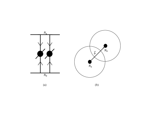
Figure 1: .Fig.1a: Parton model contribution to Double Parton Scattering of two nucleons ;Fig.1b Collision of two nucleons at the impact parameter b

In the mean field approximation, that is valid at small transverse scales of order several GeV and small x 16b , one can prove that the two particle GPDs factorize:

$${}_{2}G(x_{1},x_{2},Q_{1}^{2},Q_{2}^{2},\Delta)=_{1}G(x_{1},Q_{1}^{2},\Delta)_{1}G(x_{1},Q_{1}^{2},\Delta),$$ (3)

where ${}_{1}G$ are the conventional one particle GPD diehl ; radyushkin . The latter in the mean field approximation can be written as

$${}_{1}G(x_{1},Q_{1}^{2},\Delta)=f(x_{1},Q_{1}^{2})F_{2g}(\Delta,x_{1}),$$ (4)

where $F_{2g}$ is called a two gluon formfactor and only weakly depends on x and $Q^{2}$.

In the coordinate space we have

$${}_{1}G(x,Q^{2},\vec{r})=f(x,Q^{2})\rho(\vec{r});\rho(\vec{r})=\int d^{2}\Delta F_{2g}(\Delta,x_{1})\exp(i\vec{\Delta}\vec{r}),$$ (5)

where $\rho(\vec{r})$ is the transverse parton density. Note that in such approach the parton density is normalized by one

$$\int\rho(\vec{r})d^{2}r=1.$$ (6)

The effective cross section is then given by

$$\frac{1}{\sigma_{eff}}=\int d^{2}b(\int d^{2}r\rho(\vec{r})\rho(\vec{r}-\vec{b}))^{2},$$ (7)

where $\vec{b}$ is the impact parameter of the proton proton collision.

III The Hot Spots Model.

The hot spots mode assumes a specific type of distribution for the transverse positions of the gluonic content of the proton Mantysaari:2022ffw ; Mantysaari:2022sux . According to the model the gluons are concentrated around $N_{q}$ points, called the hot spots, positioned in the transverse positions $\vec{b}_{i}$ with a two-dimensional Gaussian distribution around the center of mass the proton, marked as $\vec{c}$, with the width $B_{p}$. The hot spots distribution around a known center is :

$$\rho\left(\left\{\vec{b}_{i}\right\}_{i=1}^{N_{q}}|\vec{c}\right)=\frac{2\pi B_{p}}{N_{q}}\delta^{\left(2\right)}\left(\frac{\sum_{i=1}^{N_{q}}\vec{b}_{i}}{N_{q}}-\vec{c}\right)\left(\prod_{i=1}^{N_{q}}\frac{1}{2\pi B_{p}}e^{-\frac{\left(\vec{b}_{i}-\vec{c}\right)^{2}}{2B_{p}}}\right),$$ (8)

where the normalization factor of $2\pi B_{p}/N_{q}$ is chosen to get a total integral of one. Each hot spot has the Gaussian density around the center of the hot spot with a width of $B_{q}$ and can have a fluctuating strength denote as $p_{i}$. Hence, the probability distribution to have a hard parton at position $\vec{r}$ is given by:

$$\rho\left(\vec{r},\left\{\vec{b}_{i},p_{i}\right\}_{i=1}^{N_{q}}|\vec{c}\right)=\frac{2\pi B_{p}}{N_{q}}\delta^{\left(2\right)}\left(\frac{\sum_{i=1}^{N_{q}}\vec{b}_{i}}{N_{q}}-\vec{c}\right)\left(\prod_{i=1}^{N_{q}}\frac{1}{2\pi B_{p}}e^{-\frac{b_{i}^{2}}{2B_{p}}}\right)\left(\frac{1}{N_{q}}\sum_{i=1}^{N_{q}}p_{i}\frac{1}{2\pi B_{q}}e^{-\frac{\left(\vec{r}-\vec{b}_{i}\right)^{2}}{2B_{q}}}\right).$$ (9)

Here the hot spot strengths $p_{i}$ are assumed to have random distribution

$$P(\log(p_{i}))=\frac{1}{\sqrt{2\pi}}\exp(-\log(p_{i})^{2}/2\sigma^{2}),$$ (10)

so that $\bar{p}_{i}\equiv E(p_{i})$ -average value of $p_{i}$ is equal to $\exp(\sigma^{2}/2)$, and overall normalisation is chosen to ensure normalization condition 6.

Using the distribution 10 we obtain for the average value of $p^{n}$ $E(p^{n})$

$$E\left[p^{n}\right]=e^{\frac{n^{2}\sigma^{2}}{2}}.$$ (11)

Note that if we take into account the fluctuating strength in order to satisfy the normalization condition (6) we would have to divide the average density by factor $E(p)$ and the product of four densities that appears in the formula for the cross section by

$$E\left[p\right]^{4}=e^{2\sigma^{2}}.$$ (12)

IV Calculating the DPS Effective Cross-Section.

In order to calculate the effective cross section we need to calculate the event by event cross section for given positions of hot spots and impact parameter $\vec{b}$, and the hot spot strenghts using eq. 7, and then average over the hot spot positions, impact parameter and hot spot strengths. The average of the hot spots positions is done by taking an integral over the positions of the hot-spots, marked as $\left\{\vec{a}_{i},\vec{b}_{j}\right\}_{i,j=1}^{N_{q}}$ in addition to the collision impact parameter $\vec{b}$. Next we shall average over the hot spot strength fluctuations using Eqs. 10,11,12.

We start by finding the convolution of the single hot spot collision, obtaining the following integral:

$$\int d^{2}r\rho\left(\vec{r},\left\{\vec{a}_{i}\right\}_{i=1}^{N_{q}},\vec{c}\right)\rho\left(\vec{r},\left\{\vec{b}_{j}\right\}_{j=1}^{N_{q}},\vec{c}+\vec{b}\right) \propto \sum_{i,j}\int d^{2}re^{-\frac{\left(\vec{r}-\vec{a}_{i}\right)^{2}+\left(\vec{r}-\vec{b}_{j}\right)^{2}}{2B_{q}}}$$ (13)

$$= \pi B_{q}\sum_{i,j}e^{-\frac{\left(\vec{a}_{i}-\vec{b}_{j}\right)^{2}}{4B_{q}}}.$$

This integral is proportional to the probability for a single hard partonic process to occur for general positions of the hot spots. Taking the square of this expression and integrating it over the hot spots positions to find $\left(\sigma_{eff}\right)^{-1}$. To do that we need to separate the sums into three different classes. If the positions of the hot spots are marked as $\vec{a}_{i_{1}},\;\vec{a}_{i_{2}},\;\vec{b}_{j_{1}}$ and $\vec{b}_{j_{2}}$ we write the classes as (Fig.2):

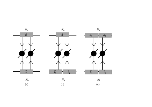
Figure 2: Three distinct classes of diagrams for DPS scattering in the hot spots model

• Class I: The two partons come from one hot spot for both protons, or $i_{1}=i_{2}$ and $j_{1}=j_{2}$.

• Class II: One proton emits the two partons from a single hot spot while the other emits them from two different hot-spots, or $i_{1}=i_{2}$ and $j_{1}\neq j_{2}$ or $i_{1}\neq i_{2}$ and $j_{1}=j_{2}$.

• Class III: Each proton emits the two partons from different hot spots, or $i_{1}\neq i_{2}$ and $j_{1}\neq j_{2}$.

In addition to separating the sums into cases we also use change the delta function to a form more convenient in the present calculation:

$$\delta^{\left(2\right)}\left(\frac{\sum_{i=1}^{N_{q}}\vec{a}_{i}}{N_{q}}-\vec{c}\right)\delta^{\left(2\right)}\left(\frac{\sum_{j=1}^{N_{q}}\vec{b}_{j}}{N_{q}}-\left(\vec{c}+\vec{b}\right)\right)=\int\frac{d^{2}s_{1}d^{2}s_{2}}{\left(2\pi\right)^{4}}e^{i\vec{s}_{1}\cdot\left(\frac{\sum_{i=1}^{N_{q}}\vec{a}_{i}}{N_{q}}-\vec{c}\right)}e^{i\vec{s}_{2}\cdot\left(\frac{\sum_{j=1}^{N_{q}}\vec{b}_{j}}{N_{q}}-\left(\vec{c}+\vec{b}\right)\right)}$$ (14)

We also need the integral over a hot spot that isn’t part of the collision, it is simply:

$$I\left(\vec{c},\vec{s}\right)\equiv\int d^{2}b_{j}e^{\frac{i}{N_{q}}\vec{s}\cdot\vec{b}_{j}-\frac{\left(\vec{b}_{j}-\vec{c}\right)^{2}}{2B_{p}}}=2\pi B_{p}e^{-\frac{B_{p}}{2N_{q}^{2}}s^{2}+i\frac{1}{N_{q}}\vec{s}\cdot\vec{c}},$$ (15)

and the total constant factor is $\left(\left(2\pi\right)^{2}N_{q}^{2}\left(2\pi B_{p}\right)^{N_{q}-1}\left(2\pi B_{q}\right)\right)^{-2}$, we also set the center of the first proton to be $\vec{c}=\vec{0}$ and the second is then $\vec{c}+\vec{b}=\vec{b}$.

IV.1 Two Partons From a Single hot spot Of Each Proton

In case I the two sums become:

$$\left(\sum_{i_{1},j_{1}}p_{i_{1}}\tilde{p}_{j_{1}}e^{-\frac{\left(\vec{a}_{i_{1}}-\vec{b}_{j_{1}}\right)^{2}}{4B_{q}}}\right)\left(\sum_{i_{2},j_{2}}p_{i_{2}}\tilde{p}_{j_{2}}e^{-\frac{\left(\vec{a}_{i_{2}}-\vec{b}_{j_{2}}\right)^{2}}{4B_{q}}}\right)\rightarrow p^{2}\tilde{p}^{2}{N_{q}}^{2}e^{-\frac{\left(\vec{a}_{1}-\vec{b}_{1}\right)^{2}}{2B_{q}}},$$ (16)

where we get a factor of $N_{q}^{2}$ from choosing a single hot spot in each proton without loss of generality and $\tilde{p}$ represent the hot spot strength from the $b$ proton. The $2N_{q}-2$ hot spots in two nucleons that are not involved in the interaction give us a factor of $\left(I\left(\vec{0},\vec{s}_{1}\right)I\left(\vec{b},\vec{s}_{2}\right)\right)^{N_{q}-1}$. We are left with the following integral:

$$A=\frac{p^{2}\tilde{p}^{2}}{4N_{q}^{4}\left(2\pi\right)^{6}B_{q}^{2}}\int d^{2}bd^{2}s_{1}d^{2}s_{2}d^{2}a_{1}d^{2}b_{1}e^{-\frac{\left(N_{q}-1\right)B_{p}}{2N_{q}^{2}}\left(s_{1}^{2}+s_{2}^{2}\right)-i\frac{1}{N_{q}}\vec{s}_{2}\cdot\vec{B}-\frac{\left(\vec{a}_{1}-\vec{b}_{1}\right)^{2}}{2B_{q}}+\frac{i}{N_{q}}\left[\vec{s}_{1}\cdot\vec{a}_{1}+\vec{s}_{2}\cdot\vec{b}_{1}\right]-\frac{a^{2}+\left(\vec{b}_{1}-\vec{b}\right)^{2}}{2B_{p}}}.$$ (17)

We are left with a $10$-dimensional Gaussian, but really, the two Cartesian coordinates are completely separable so really we can write integral $A$ as the square of a $5$-dimensional Gaussian. If we write the parameters as a vector $\vec{x}^{T}=\left(a_{1x},b_{1x},b_{x},s_{1x},s_{2x}\right)$ we obtain:

$$A=\frac{p^{2}\tilde{p}^{2}}{4N_{q}^{4}\left(2\pi\right)^{6}B_{q}^{2}}\left(\int d^{5}xe^{-\vec{x}^{T}M_{A}\vec{x}}\right)^{2},$$ (18)

with $M$ being the following symmetric matrix:

$$M_{A}=\left(\begin{array}[]{ccccc}\frac{B_{p}+B_{q}}{2B_{p}B_{q}}&-\frac{1}{2B_{q}}&0&-\frac{i}{2N_{q}}&0\\ -\frac{1}{2B_{q}}&\frac{B_{p}+B_{q}}{2B_{p}B_{q}}&-\frac{1}{2B_{p}}&0&-\frac{i}{2N_{q}}\\ 0&-\frac{1}{2B_{p}}&\frac{1}{2B_{p}}&0&\frac{i}{2N_{q}}\\ -\frac{i}{2N_{q}}&0&0&\frac{N_{q}-1}{2N_{q}^{2}}B_{p}&0\\ 0&-\frac{i}{2N_{q}}&\frac{i}{2N_{q}}&0&\frac{N_{q}-1}{2N_{q}^{2}}B_{p}\end{array}\right),$$ (19)

and we can use the Gaussian formula $\int d^{n}xe^{-\vec{x}^{T}M\vec{x}}=\frac{\left(2\pi\right)^{n/2}}{\sqrt{\det M}}$ to get:

$$A=\frac{p^{2}\tilde{p}^{2}}{8\pi B_{q}{N_{q}}^{2}}.$$ (20)

Averaging over $p$ and $\tilde{p}$ we obtain:

$$A=\frac{E\left[p^{2}\right]^{2}}{8\pi B_{q}{N_{q}}^{2}}=\frac{e^{4\sigma^{2}}}{8\pi B_{q}{N_{q}}^{2}}.$$ (21)

This expression takes into account fluctuations of the hot spot strength. If we neglect the fluctuations of the hot spot strength, which corresponds to setting $\sigma=0$, we would get:

$$A_{\sigma=0}=\frac{1}{8\pi B_{q}{N_{q}}^{2}}.$$ (22)

IV.2 Two Partons From a Single Hot Spot Of One Proton And Two Different Hot Spots From The Other Proton

In case II the two sums become one of two sub-cases, for $i_{1}=i_{2}$ but $j_{1}\neq j_{2}$ we get:

$$\left(\sum_{i_{1},j_{1}}p_{i_{1}}\tilde{p}_{j_{1}}e^{-\frac{\left(\vec{a}_{i_{1}}-\vec{b}_{j_{1}}\right)^{2}}{4B_{q}}}\right)\left(\sum_{i_{2},j_{2}}p_{i_{2}}\tilde{p}_{j_{2}}e^{-\frac{\left(\vec{a}_{i_{2}}-\vec{b}_{j_{2}}\right)^{2}}{4B_{q}}}\right)\rightarrow p^{2}\tilde{p}_{1}\tilde{p}_{2}{N_{q}}^{2}\left(N_{q}-1\right)e^{-\frac{\left(\vec{a}_{1}-\vec{b}_{1}\right)^{2}+\left(\vec{a}_{1}-\vec{b}_{2}\right)^{2}}{4B_{q}}},$$ (23)

where the factor of ${N_{q}}^{2}\left(N_{q}-1\right)$ comes from choosing the hot spots without loss of generality. In this sub-case, we also get a factor of $\left(I\left(\vec{0},\vec{s}_{1}\right)\right)^{N_{q}-1}\left(I\left(\vec{b},\vec{s}_{2}\right)\right)^{N_{q}-2}$, leaving us with the integral:

$$B_{1}=\frac{\left(N_{q}-1\right)p^{2}\tilde{p}_{1}\tilde{p}_{2}}{2N_{q}^{5}\left(2\pi\right)^{7}B_{p}B_{q}^{2}}\left(\int d^{6}xe^{-\vec{x}^{T}M_{B_{1}}\vec{x}}\right)^{2},$$ (24)

where now $\vec{x}^{T}=\left(a_{1x},b_{1x},b_{2x},b_{x},s_{1x},s_{2x}\right)$ and:

$$M_{B_{1}}=\left(\begin{array}[]{cccccc}\frac{B_{p}+B_{q}}{2B_{p}B_{q}}&-\frac{1}{4B_{q}}&-\frac{1}{4B_{q}}&0&-\frac{i}{2N_{q}}&0\\ -\frac{1}{4B_{q}}&\frac{B_{p}+2B_{q}}{4B_{p}B_{q}}&0&-\frac{1}{2B_{p}}&0&0\\ -\frac{1}{4B_{q}}&0&\frac{B_{p}+2B_{q}}{4B_{p}B_{q}}&-\frac{1}{2B_{p}}&0&-\frac{i}{2N_{q}}\\ 0&-\frac{1}{2B_{p}}&-\frac{1}{2B_{p}}&\frac{1}{B_{p}}&0&-\frac{i}{2N_{q}}\\ -\frac{i}{2N_{q}}&0&0&0&\frac{N_{q}-1}{2N_{q}^{2}}B_{p}&\frac{i}{N_{q}}\\ 0&0&-\frac{i}{2N_{q}}&-\frac{i}{2N_{q}}&\frac{i}{N_{q}}&\frac{N_{q}-2}{2N_{q}^{2}}B_{p}\end{array}\right).$$ (25)

Using the Gaussian formula we get

$$B_{1}=\frac{\left(N_{q}-1\right)p^{2}\tilde{p}_{1}\tilde{p}_{2}}{4\pi\left(B_{p}+2B_{q}\right)N_{q}^{2}}.$$ (26)

For the second sub-case, $i_{1}\neq i_{2}$ and $j_{1}=j_{2}$, it can be shown that we get the same constant factor but a different matrix, but overall the determinants are the same so we get $B_{2}=B_{1}\Rightarrow B=2B_{1}$. The average over the hot spots strengths gives the final expression for this case:

$$B=\frac{\left(N_{q}-1\right)E\left[p^{2}\right]E\left[p\right]^{2}}{2\pi\left(B_{p}+2B_{q}\right){N_{q}}^{2}}=\frac{\left(N_{q}-1\right)e^{3\sigma^{2}}}{2\pi\left(B_{p}+2B_{q}\right){N_{q}}^{2}},$$ (27)

In the case when fluctuations of the hot spot strength are neglected $\sigma=0$ we obtain:

$$B_{\sigma=0}=\frac{\left(N_{q}-1\right)}{2\pi\left(B_{p}+2B_{q}\right){N_{q}}^{2}}.$$ (28)

IV.3 Two Different Hot Spots From Both Protons

In the case II the two sums become one of two sub-cases. For $i_{1}\neq i_{2}$ but $j_{1}\neq j_{2}$ we get for the sums :

$$\left(\sum_{i_{1},j_{1}}p_{i_{1}}\tilde{p}_{j_{1}}e^{-\frac{\left(\vec{a}_{i_{1}}-\vec{b}_{j_{1}}\right)^{2}}{4B_{q}}}\right)\left(\sum_{i_{2},j_{2}}p_{i_{2}}\tilde{p}_{j_{2}}e^{-\frac{\left(\vec{a}_{i_{2}}-\vec{b}_{j_{2}}\right)^{2}}{4B_{q}}}\right)\rightarrow p_{1}\tilde{p}_{1}p_{2}\tilde{p}_{2}N_{q}^{2}\left(N_{q}-1\right)^{2}e^{-\frac{\left(\vec{a}_{1}-\vec{b}_{1}\right)^{2}+\left(\vec{a}_{2}-\vec{b}_{2}\right)^{2}}{4B_{q}}},$$ (29)

with a factor of $\left(I\left(\vec{0},\vec{s}_{1}\right)I\left(\vec{b},\vec{s}_{2}\right)\right)^{N_{q}-2}$ we get the integral to be:

$$C=\frac{p_{1}\tilde{p}_{1}p_{2}\tilde{p}_{2}\left(N_{q}-1\right)^{2}}{4N_{q^{4}}\left(2\pi\right)^{8}B_{p}^{2}B_{q}^{2}}\left(\int d^{7}xe^{-\vec{x}^{T}M_{C}\vec{x}}\right)^{2},$$ (30)

with the vectors being $\vec{x}^{T}=\left(a_{1x},a_{2x},b_{1x},b_{2x},b_{x},s_{1x},s_{2x}\right)$ and the matrix:

$$M_{C}=\left(\begin{array}[]{ccccccc}\frac{B_{p}+2B_{q}}{4B_{p}B_{q}}&0&-\frac{1}{4B_{q}}&0&0&-\frac{i}{2N_{q}}&0\\ 0&\frac{B_{p}+2B_{q}}{4B_{p}B_{q}}&0&-\frac{1}{4B_{q}}&0&-\frac{i}{2N_{q}}&0\\ -\frac{1}{4B_{q}}&0&\frac{B_{p}+2B_{q}}{4B_{p}B_{q}}&0&-\frac{1}{2B_{p}}&0&-\frac{i}{2N_{q}}\\ 0&-\frac{1}{4B_{q}}&0&\frac{B_{p}+2B_{q}}{4B_{p}B_{q}}&-\frac{1}{2B_{p}}&0&-\frac{i}{2N_{q}}\\ 0&0&-\frac{1}{2B_{p}}&-\frac{1}{2B_{p}}&\frac{1}{B_{p}}&0&\frac{i}{N_{q}}\\ -\frac{i}{2N_{q}}&-\frac{i}{2N_{q}}&0&0&0&\frac{N_{q}-2}{2N_{q}^{2}}B_{p}&0\\ 0&0&-\frac{i}{2N_{q}}&-\frac{i}{2N_{q}}&\frac{i}{N_{q}}&0&\frac{N_{q}-2}{2N_{q}^{2}}B_{p}\end{array}\right).$$ (31)

Using the Gaussian formula we get:

$$C=\frac{p_{1}\tilde{p}_{1}p_{2}\tilde{p}_{2}\left(N_{q}-1\right)^{2}}{8\pi\left(B_{p}+B_{q}\right)N_{q}^{2}},$$ (32)

average over the hot spots strength gives us the final form for this case:

$$C=\frac{E\left[p\right]^{4}\left(N_{q}-1\right)^{2}}{8\pi\left(B_{p}+B_{q}\right)N_{q}^{2}}=\frac{\left(N_{q}-1\right)^{2}e^{2\sigma^{2}}}{8\pi\left(B_{p}+B_{q}\right)N_{q}^{2}},$$ (33)

If the fluctuations of the hot spot strength are neglected, $\sigma=0$ and we obtain

$$C_{\sigma=0}=\frac{\left(N_{q}-1\right)^{2}}{8\pi\left(B_{p}+B_{q}\right)N_{q}^{2}}.$$ (34)

V Total Effective Cross section and conclusions.

Putting together our results in Eq. 12, Eq. 21, Eq. 27, and Eq. 33 we find $\sigma_{eff}$ to be:

$$\sigma_{eff}=\left(A+B+C\right)^{-1}=\frac{8\pi N_{q}^{2}}{\frac{e^{2\sigma^{2}}}{B_{q}}+\frac{4\left(N_{q}-1\right)e^{\sigma^{2}}}{B_{p}+2B_{q}}+\frac{\left(N_{q}-1\right)^{2}}{B_{p}+B_{q}}}.$$ (35)

Here we normalized the gluon density to one according Eq. 6 using Eq.12.

Using the parameters from table I in Mantysaari:2022ffw , which for convenience we present here as Table 1, we get two possible values for $\sigma_{eff}$:

Parameter	Description	Variable $N_{q}$	$N_{q}\equiv 3$
$N_{q}$	Number of hot spots	$6.79_{-4.83}^{+2.93}$	$3$
$\sigma$	Magnitude of hot spots strength fluctuations	$0.833_{-0.441}^{+0.194}$	$0.563_{-0.141}^{+0.143}$
$B_{q}\left[GeV^{-2}\right]$	Hot spot size	$0.474_{-0.286}^{+0.434}$	$0.346_{-0.202}^{+0.282}$
$B_{p}\left[GeV^{-2}\right]$	Proton size	$4.02_{0.728}^{+1.73}$	$4.45_{-0.803}^{+0.801}$

Table 1: The four parameters used in our calculations as taken from Mantysaari:2022ffw for the case of Variable $N_{q}$ and $N_{q}\equiv 3$

$$\sigma_{eff}\approx 17\,\,{\rm mb}\,\,\,{\rm for}N_{q}=7,$$

$$\sigma_{eff}\approx 10.5{\rm mb}\,\,{\rm for}N_{q}=3.$$

(36)

We see that the hot spot model with hot spot strength fluctuations taken into account, and especially for $N_{q}=3$ leads to substantially larger cross section of the DPS process than obtained from experimental data ATLAS ; CMS (BS for recent review).

Moreover , note that $\sigma_{eff}\sim 20$ mb is obtained for virtualities of $\sim\approx 20$ GeV and higher for hard processes. In order to obtain the values of $\sigma_{eff}$ at scales of order several GeV one needs to carry inverse DGLAP evolution leading to $\sigma_{eff}=$ 25-35 mb . The latter number is similar to the value of $\sigma_{eff}$ used in MC generators PYTHIA ; HERWIG for moderate $p_{t}$ of several GeV. Thus the inclusion of pQCD evolution only increases the tension.

If we look at the case with $\sigma=0$,i.e. neglect the hot spot strength fluctuations we obtain that for the set with variable $N_{q}$ we find $\sigma_{eff}\approx 32mb$, and for the set with a set $N_{q}\equiv 3$ we get $\sigma_{eff}\approx 17mb$. Thus if we neglect hot spot strength fluctuations, the DPS rate is consistent with the experimental data, however it will be still in tension for $N_{q}=3$ if we take into account the $Q^{2}$ pQCD evolution. On the other hand if we increase the hot spot number the DPS cross section decreases and is consistent with the current DPS data.

In conclusion we see that DPS information can be used as an effective constraint on the models of the nucleon structure.

References

• (1) R. Abdul Khalek et. al., Science Requirements and Detector Concepts for the Electron-Ion Collider: EIC Yellow Report, arXiv:2103.05419 [physics.ins-det].
• (2) B. Blok and M. Strikman, Adv. Ser. Direct. High Energy Phys. 29 (2018), 63-99. [arXiv:1709.00334 [hep-ph]].
• (3) E. M. Levin, L. L. Frankfurt, UFN, 94 (1968), 243–288; Sov. Phys. Usp., 11 (1968), 106–129.
• (4) A. H. Mueller, Nucl. Phys. B Proc. Suppl. 18 (1991), 125-132.
• (5) H. Mäntysaari, B. Schenke Phys.Lett.B 772 (2017) 832-838 • e-Print: 1703.09256 [hep-ph].
• (6) H. Mäntysaari, B. Schenke, C. Shen and W. Zhao, Phys. Lett. B 833 (2022), 137348.
• (7) H. Mäntysaari, F. Salazar and B. Schenke, Phys. Rev. D 106 (2022) no.7, 074019. [arXiv:2207.03712 [hep-ph]].
• (8) M. L. Good and W. D. Walker, Phys. Rev. 120 (1960), 1857-1860.
• (9) L. Frankfurt, V. Guzey, A. Stasto and M. Strikman, Rept. Prog. Phys. 85 (2022) no.12, 126301 [arXiv:2203.12289 [hep-ph]].
• (10) N. Paver and D. Treleani, Z. Phys. C 28 (1985), 187.
• (11) M. Mekhfi, Phys. Rev. D 32 (1985), 2371.
• (12) J.R. Gaunt and W.J. Stirling, JHEP 1003, 005 (2010) ,[arXiv:0910.4347 [hep-ph]].
• (13) B. Blok, Yu. Dokshitzer, L. Frankfurt and M. Strikman, Phys. Rev.  D 83, 071501 (2011) [arXiv:1009.2714 [hep-ph]].
• (14) M. Diehl, PoS D IS2010 (2010) 223 [arXiv:1007.5477 [hep-ph]].
• (15) J.R. Gaunt and W.J. Stirling, JHEP 1106, 048 (2011) [arXiv:1103.1888 [hep-ph]].
• (16) B. Blok, Yu. Dokshitser, L. Frankfurt and M. Strikman, Eur. Phys. J. C 72, 1963 (2012) [arXiv:1106.5533 [hep-ph]].
• (17) M. Diehl, D. Ostermeier and A. Schafer, JHEP 1203 (2012) 089 [arXiv:1111.0910 [hep-ph]].
• (18) B. Blok, Y. Dokshitzer, L. Frankfurt and M. Strikman, Eur. Phys. J. C 74 (2014) 2926 [arXiv:1306.3763 [hep-ph]].
• (19) M. Diehl, J. R. Gaunt and K. Schönwald, JHEP 1706 (2017) 083 [arXiv:1702.06486 [hep-ph]].
• (20) A. V. Manohar and W. J. Waalewijn, Phys. Rev. D 85 (2012) 114009.
• (21) O. Kuprash [ATLAS], “Studies of the underlying-event properties and of hard double parton scattering with the ATLAS detector,” PoS DIS2017 (2018), 035.
• (22) R. Gupta [CMS and TOTEM], “Double parton scattering studies in CMS,” PoS EPS-HEP2021 (2022), 335.
• (23) M. Diehl, Phys. Rept. 388 (2003), 41-277 [arXiv:hep-ph/0307382 [hep-ph]].
• (24) A. V. Belitsky and A. V. Radyushkin, Phys. Rept. 418 (2005), 1-387 [arXiv:hep-ph/050400.
• (25) T. Sjöstrand, Adv. Ser. Direct. High Energy Phys. 29 (2018), 191-225 [arXiv:1706.02166 [hep-ph]].
• (26) J. Bellm, S. Gieseke and P. Kirchgaesser, Eur. Phys. J. C 80 (2020) no.5, 469 [arXiv:1911.13149 [hep-ph]].