Reflectionless potentials and resonant scattering of flat-top and thin-top solitons

Abstract

We identify a class of potentials for which the scattering of flat-top solitons and thin-top solitons of the nonlinear Schrödinger equation with dual nonlinearity can be reflectionless. The scattering is characterized by sharp resonances between regimes of full transmission and full quantum reflection. Perturbative expansion in terms of the magnitude of radiation losses leads to the general form of reflectionless potentials. Simulating the scattering of flat-top solitons and thin-top solitons confirms the reflectionless feature of these potentials.

I Introduction

The unique features of solitons are exhibited most clearly upon their scattering by external potentials. The so-called reflectionless scattering is one such striking example. Scattering of solitons by specific types of potentials is characterized by the complete absence of radiation and by preserving the integrity of solitons after scattering goodman . Moreover, the interesting phenomena of quantum reflection and resonant scattering are usually studied with reflectionless potentials lee ; ernst . A well-known and well-studied example is the scattering of bright solitons of the nonlinear Schrödinger equation (NLSE) by the reflectionless Pöschl-Teller potential well goodman ; lee .

On the fundamental level, resonant scattering by reflectionless potentials reveals the spectrum of the potential’s bound states LU . Reflectionless scattering is also important for applications in optical data processing where optical devises may be designed to simulate certain functions such as switching, routing, unidirectional flow, and logic gating hasegawa ; asad ; usama1 ; usama2 .

Stimulated by the recent experimental realization of the flat-top soliton exp1 ; exp2 , which is a solution of the NLSE with dual nonlinearity, interest in such kind of solitonic excitations has been growing cheiney ; bottcher ; luo ; khare ; usama3 ; debnath ; petrov ; chen ; pathak . However, and to the best of our knowledge, the scattering properties of flat-top solitons are scarcely studied in the literature zeng ; umarov1 ; umarov2 . The present work attempts to answer three related fundamental questions: 1) Can quantum reflection occur for flat-top solitons? 2) Do reflectionless potentials exist for flat-top solitons? 3) Do flat-top solitons exhibit resonant scattering, as in bright solitons of NLSE? The rationale behind posing these questions is that flat-top solitons can be very wide, and thus it is not obvious that such a wide object may scatter off potentials without splitting or forming radiation. Nonetheless, the answer we found to all of these questions is ‘yes’.

We consider the NLSE with dual nonlinearity and then show that it supports a class of solutions that comprises a spectrum of flat-top solitons, bright solitons, kink solitons, and another type which we denote as ‘thin-top’ solitons. The spectrum of flat-top solitons is bounded by bright solitons, with vanishing width of its top, and kink solitons, with diverging width of its top. We construct a new type of reflectionless potential using the flat-top soliton and then study its scattering properties. The form of the reflectionless potential is derived using an ansatz for the scattered wave in the form of a localized soliton part and a small extended radiation part. A perturbative expansion in the small magnitude of the radiation part leads to the general form of reflectionless potential. From the spectrum of this class of solutions, a corresponding spectrum of reflectionless potentials is obtained. Simulating the scattering of flat-top and thin-top solitons by these reflectionless potentials, the reflectionless feature of the potentials will then be revealed. In addition, our simulations show that flat-top and thin-top solitons do indeed exhibit quantum reflection and resonant scattering. It should be noted that simulating flat-top solitons turns out to be numerically demanding when the soliton is very wide. Our numerical code, based on power series expansion LUcode , is shown to efficiently simulate the widest flat-top soliton possible by the machine precision.

The rest of the paper is organized as follows. In Section II, we present the exact solution of the NLSE with dual nonlinearity and discuss its properties. In Section III, we derive the reflectionless potential. In Section IV, we perform numerical simulations that confirm the reflectionless property of the potentials. In Section V, we end with our main conclusions.

II Family of solutions

The dynamics of so-called flat-top soliton is described by the following NLSE with dual nonlinearity

$$i\frac{\partial}{\partial t}\psi(x,t)=-g_{1}\,\frac{\partial^{2}}{\partial x^{2}}\psi(x,t)-g_{2}|\psi(x,t)|^{n}\psi(x,t)-g_{3}|\psi(x,t)|^{2n}\psi(x,t)+V(x)\,\psi(x,t),$$ (1)

where $\psi(x,t)$ is generally a complex field, $V(x)$ is an external potential, $g_{1}$ characterizes the strength of dispersion, $g_{2}$ and $g_{3}$ characterize the strengths of the two nonlinearities, and $n$ is an integer. For $n=2$, which we will assume for the rest of this paper, the typical NLSE with cubic and quintic nonlinearities will be retrieved, where the cubic term corresponds to the Kerr nonlinearity in the context of optical solitons and Hartree-Fock interatomic interaction in the case of Bose-Einstein condensates pethick . The flat-top soliton solution belongs to a more general class of stationary solutions which can be written in the form usamaNbahlouli ; ourbook

$$\psi(x,t)=\sqrt{\frac{2u_{0}}{g_{2}\sqrt{1+\gamma}}}\,\frac{1}{\sqrt{\frac{1-\sqrt{1+\gamma}}{2\sqrt{1+\gamma}}+{\rm cosh}^{2}\left[\sqrt{\frac{u_{0}}{g_{1}}}(x-x_{0}-v_{0}t)\right]}}\,e^{i\phi(x,t)},$$ (2)

where $u_{0}$, $x_{0}$, and $v_{0}$ are arbitrary parameters corresponding to the amplitude, peak position, and speed of the soliton, respectively, $\gamma=g_{3}/g_{30}$, where $g_{30}=3g_{2}^{2}/16u_{0}$, and $\phi(x,t)=u_{0}\,t+v_{0}[2(x-x_{0})-v_{0}\,t]/4g_{1}$. It should be noted that, although we denote this solution as stationary, we still allow for the centre-of-mass motion in order to study its scattering with potentials below. The profile is thus truly stationary only in a frame of reference moving with the soliton. For stationary solutions, the profile should be real which requires $\gamma\geq-1$. This general expression defines a spectrum of solutions containing four different nontrivial solutions, namely: bright soliton (BS), kink soliton (KS), flat-top soliton (FT), and thin-top soliton (TT). We termed the last solution as such since it turned out that its peak width is thinner than that of the bright soliton, which is the opposite case of flat-top solitons. We believe this type of soliton is not identified or studied previously in the literature. The whole spectrum of solutions can be scanned in terms of $\gamma$ values, as shown schematically in Fig. 1.

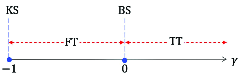
Figure 1: Schematic diagram showing the spectrum of solutions in terms of $\gamma$. The four solutions, bright soliton (BS), kink soliton (KS), flat-top soliton (FT), and thin-top soliton (TT) are given by (3), (6), (7), (8), respectively.

We list here the four different solutions. While some of these solutions are known, we include them for completeness.

I. Bright soliton, $\gamma=0$:

$$\psi(x,t)=\sqrt{\frac{2u_{0}}{g_{2}}}\,{\rm sech}\left[\sqrt{\frac{u_{0}}{g_{1}}}(x-x_{0}-v_{0}t)\right]\,e^{i\phi(x,t)},$$ (3)

II. Kink soliton, $\gamma=-1$:
Taking the limit $\gamma\rightarrow-1$ in Eq. (2), the solution takes the form of the following constant wave (CW)

$$\psi(x,t)=2\,\sqrt{\frac{u_{0}}{g_{2}}}\,e^{i\phi(x,t)}.$$ (4)

Since $x_{0}$ is an arbitrary parameter, we set $x_{0}$ as

$$x_{0}=\sqrt{\frac{g_{1}}{16u_{0}}}\,\ln{\left[\frac{g_{1}}{g_{2}^{2}(1+\gamma)}\right]},$$ (5)

which corresponds to shifting the origin such that the left side of the flat-top solution is always at $x=0$ for all values of $\gamma$. In this case the limit $\gamma\rightarrow-1$ leads to the following kink solution

$$\psi(x,t)=2\,\sqrt{\frac{u_{0}}{g_{2}}}\,\frac{1}{\sqrt{1+\sqrt{\frac{g_{1}}{4g_{2}^{2}}}\,\exp{\left(-2\sqrt{\frac{u_{0}}{g_{1}}}\,x\right)}}}\,e^{i\phi(x,t)}.$$ (6)

III. Flat-top soliton, $-1<\gamma<0$: For this range of $\gamma$, it will be convenient to express the solution using the transformation $\gamma=-\cos^{2}(\theta)$, where $0<\theta<\pi/2$

$$\psi(x,t)=2\,\sqrt{\frac{u_{0}}{g_{2}}}\,\frac{1}{\sqrt{1+\sin(\theta)\,\cosh\left[\sqrt{\frac{4u_{0}}{g_{1}}}(x-x_{0}-v_{0}t)\right]}}\,e^{i\phi(x,t)}.$$ (7)

IV. Thin-top soliton, $\gamma>0$:
In this case, the solution is expressed using the transformation $\gamma=\sinh^{2}(\theta)$, where $\theta\neq 0$

$$\psi(x,t)=2\,\sqrt{\frac{u_{0}}{g_{2}}}\,\frac{1}{\sqrt{1+\cosh(\theta)\,\cosh\left[\sqrt{\frac{4u_{0}}{g_{1}}}(x-x_{0}-v_{0}t)\right]}}\,e^{i\phi(x,t)}.$$ (8)

In Fig. 2(a), we plot these four solutions for the same set of parameters. They differ only by the value of $\gamma$ and hence their norm.

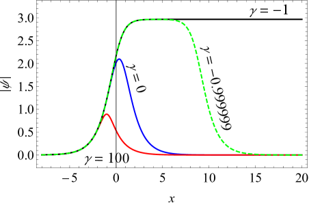
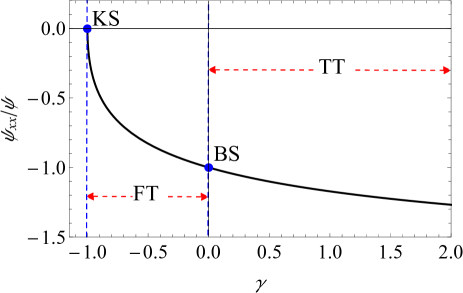
Figure 2: Family of exact solutions to Eq. (1). (a) Profiles of the four solutions (3), (6), (7), (8). (b) Curvatures of the four solutions at $x=t=0$ with $u_{0}=g_{1}=1$. Parameters used in (a): $u_{0}=2.2$, $v_{0}=0.0$, $g_{1}=3.0$, $g_{2}=1.0$, $g_{3}=\gamma\,g_{30}$, $g_{30}=3g_{2}^{2}/16u_{0}$, and $x_{0}$ is given by (5).

The central curvature of flat-top soliton is smaller than that of bright soliton. In contrast, the central curvature of the thin-top soliton is larger than that of bright soliton. In Fig. 2(b), we plot $(1/|\psi|)d^{2}|\psi|/dx^{2}$ at $x=0$. The figure shows that the curvature of flat-top solitons is always smaller than that of the bright soliton, and the curvature of thin-top solitons is always larger than the curvature of the bright soliton. The fundamental difference between flat-top soliton and thin-top soliton can be also clearly seen upon comparing them when they have the same norm. Normalising the general solution as

$$n_{0}=\int_{-\infty}^{\infty}|\psi(x,t)|^{2}dx=\frac{8g_{1}}{g_{2}}\,\sqrt{\frac{u_{0}}{g_{1}\,\gamma}}\,\tan^{-1}\left(\frac{\sqrt{1+\gamma}-1}{\sqrt{\gamma}}\right),$$ (9)

and then solving for $u_{0}$,

$$u_{0}=\frac{g_{2}^{2}n_{0}^{2}\gamma}{64g_{1}\,\left[\tan^{-1}\left(\frac{\sqrt{1+\gamma}-1}{\sqrt{\gamma}}\right)\right]^{2}},$$ (10)

the general solution (2), and hence the special solutions (3), (4), (6), (7), (8), will be normalised to $n_{0}$. In Fig. 3, we plot the normalised flat-top and thin-top solitons together with the bright soliton for the purpose of comparison.

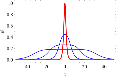
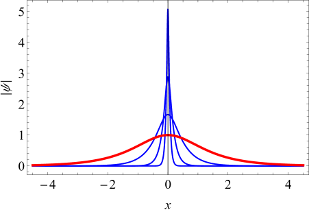
Figure 3: (a) Flat-top solitons, given by (7), with $\gamma=\{-0.99,-0.9999,-0.999999\}$, such that the last value corresponds to the widest soliton, and (b) thin-top solitons, given by (8), for $\gamma=\{9,99,999\}$, such that the last value corresponds to the thinnest soliton. Thick (red) curves correspond to the bright soliton solution for $\gamma=0$. Parameters used in both (a) and (b): $u_{0}=2.2$, $v_{0}=0.0$, $g_{1}=3.0$, $g_{2}=1.0$, $g_{3}=\gamma\,g_{30}$, $g_{30}=3g_{2}^{2}/16u_{0}$.

The figure shows that flat-top solitons are indeed always wider than the bright soliton and they become wider for values of $\gamma$ approaching $-1$, and thin-top solitons are always thinner than the bright soliton and they become thinner as $\gamma$ approaches $\infty$.

Finally, a statement about the stability of these solitons is in order. According to the Vakhitov-Kolokolov (VK) stability criterion vakhitov , the soliton with profile $\psi(x,t)=\phi(x)e^{-i\omega\,t}$, will be stable if the condition $\partial n_{0}/\partial\omega<0$ is satisfied. Applying this criterion on solution (2), where $\omega=-u_{0}$, we get

$$\frac{\partial}{\partial\omega}n_{0}=-\frac{4}{g_{2}}\,\sqrt{-\frac{g_{1}}{\omega}}\,\frac{\tan^{-1}\left(\frac{\sqrt{1+\gamma}-1}{\sqrt{\gamma}}\right)}{\sqrt{\gamma}}.$$ (11)

For $g_{1},\,g_{2}>0$ and $\omega<0$, this expression is negative for $\gamma\geq-1$, which indicates that all types of solitons mentioned above are stable according to the VK criterion.

In the next section, we derive the reflectionless potentials corresponding to the above solutions.

III Reflectionless potentials

Reflectionless scattering is defined by the absence of radiation. The scattering outcome is then assumed to be in the form of a localized solitonic part that is immersed in a weak oscillatory part, which accounts for radiation. A perturbative approach will then lead to the specific form of potential for which radiation is vanishingly small. The ansatz for the scattering outcome is written as

$$\psi_{out}(x,t)=\left[\psi_{0}(x)+\psi_{1}(x,t)\right]\,e^{i\lambda t},$$ (12)

where $\psi_{0}(x)\,e^{i\lambda t}$ is the stationary solitonic part and $\psi_{1}(x,t)$ is the small radiation part, such that $|\psi_{1}|\ll|\psi_{0}|$. The solitonic part corresponds to either reflected or transmitted soliton long after the scattering event such that the effect of the finite-range potential is absent. Substituting this ansatz in (1), the zeroth order vanishes assuming that $\psi_{0}(x)$ is a solution of the time-independent version of (1), namely

$$g_{1}\,\psi_{0}^{\prime\prime}(x)+g_{2}\,\psi_{0}^{3}(x)+g_{3}\,\psi_{0}^{5}(x)-\left(V(x)+\lambda\right)\,\psi_{0}(x)=0.$$ (13)

Since we consider a situation where the soliton after scattering is far from the potential $V(x)$, the soliton solution $\psi_{0}(x)$ may be taken as the solution of the fundamental version of (1), i.e., Eq. (13) with $V(x)=0$. The linear order gives

$$i\frac{\partial}{\partial t}\psi_{1}(x,t)+g_{1}\frac{\partial^{2}}{\partial x^{2}}\psi_{1}(x,t)+\left[g_{2}\,\psi_{0}^{2}(x)+g_{3}\,\psi_{0}^{4}(x)-(V(x)+\lambda)\right]\,\psi_{1}(x,t)+\left(2g_{3}\,\psi_{0}^{4}+g_{2}\,\psi_{0}^{2}\right){\psi_{1}}^{*}(x,t)=0.$$ (14)

In terms of the real and imaginary parts of $\psi_{1}(x,t)$, defined by $\psi_{1}(x,t)=\psi_{1r}(x,t)+i\,\psi_{1i}(x,t)$, the real and imaginary parts of the last equation give

$$g_{1}\,\frac{\partial^{2}}{\partial x^{2}}\psi_{1r}-\,\frac{\partial}{\partial t}\psi_{1i}+\left[5g_{3}\,\psi_{0}^{4}+3g_{2}\,\psi_{0}^{2}-(V(x)+\lambda)\right]\psi_{1r}=0,$$ (15)

$$g_{1}\,\frac{\partial^{2}}{\partial x^{2}}\psi_{1i}+\frac{\partial}{\partial t}\psi_{1r}+\left[g_{3}\,\psi_{0}^{4}+g_{2}\,\psi_{0}^{2}-(V(x)+\lambda)\right]\psi_{1i}=0.$$ (16)

We set the oscillatory perturbations in the form

$$\psi_{1r}(x,t)=u\cos(k\,x+\omega t),$$ (17)

and

$$\psi_{1i}(x,t)=v\sin(k\,x+\omega t),$$ (18)

where $u$ and $v$ are arbitrary amplitudes. Substituting back in Eqs. (15) and (16), a nontrivial solution requires

$$V(x)=-\left[g_{1}\,k^{2}+\lambda-2g_{2}\,\psi_{0}^{2}(x)-3g_{3}\,\psi_{0}^{4}(x)\pm\sqrt{\omega^{2}+g_{2}^{2}\,\psi_{0}^{4}(x)+4g_{2}\,g_{3}\,\psi_{0}^{6}(x)+4g_{3}^{2}\,\psi_{0}^{8}(x)}\right].$$ (19)

In the long-wavelength limit, $k,\,\omega\rightarrow 0$, the last equation reduces to

$$V(x)=g_{2}\,\psi_{0}^{2}(x)+g_{3}\,\psi_{0}^{4}(x),$$ (20)

or

$$V(x)=3g_{2}\,\psi_{0}^{2}(x)+5g_{3}\,\psi_{0}^{4}(x),$$ (21)

where we have also set $\lambda=0$ since it corresponds to a constant shift in energy. In the absence of the quintic nonlinearity, the above result should lead to the well-known case of Pöschl-Teller reflectionless potential, namely

$$V(x)=-2\,u_{0}\,{\rm sech^{2}\left(\sqrt{{\it u}_{0}/g_{1}}{\it x}\right)}.$$ (22)

Using the bright soliton solution $\psi_{0}(x)=\sqrt{2\,{\it u}_{0}/g_{2}}\,{\rm sech}(\sqrt{u_{0}/g_{1}}{\it x})$ in Eqs. (20) and (21) gives $V(x)=2\,u_{0}\,{\rm sech}^{2}\left(\sqrt{{\it u}_{0}/g_{1}}{\it x}\right)$, and $V(x)=6\,u_{0}\,{\rm sech}^{2}\left(\sqrt{{\it u}_{0}/g_{1}}{\it x}\right)$, respectively. We conjecture that what matters for the reflectionless feature is the structure of the potential such that a prefactor will not affect this property. This is based on our numerical simulations. Our perturbative calculation, in this case, accounts for the structure of the reflectionless potential but does not explain the freedom in the parameters. With this interpretation, the Pöschl-Teller potential is obtained from our results by multiplying the potential expressions we obtained by an arbitrary overall parameter that can be adjusted to get the right sign and magnitude. Indeed, our simulations show that the reflectionless property is not restricted to the parameters of the model we are solving, namely Eq. (1). The potential can thus be constructed by another solution that has the same shape but with different parameters, namely $\psi_{0p}(x)=\sqrt{2\,{\it u}_{0p}/g_{2p}}\,{\rm sech}(\sqrt{{\it u}_{0p}/g_{1p}}{\it x})$, where $g_{1p}$, $g_{2p}$, and $u_{0p}$ are arbitrary parameters that may be different than $g_{1}$, $g_{2}$, and $u_{0}$.

Similarly, a reflectionless potential for flat-top and thin-top solitons is obtained by extracting $\psi_{0}(x)$ from (2) and substituting in (19), which is then simplified as

$$V(x)=-\frac{2u_{0}}{\sqrt{1+\gamma}}\,\frac{\frac{3\gamma}{8\sqrt{1+\gamma}}+\frac{1-\sqrt{1+\gamma}}{2\sqrt{1+\gamma}}+\cosh^{2}\left(\sqrt{\frac{u_{0}}{g_{1}}}x\right)}{\left[\frac{1-\sqrt{1+\gamma}}{2\sqrt{1+\gamma}}+\cosh^{2}\left(\sqrt{\frac{u_{0}}{g_{1}}}x\right)\right]^{2}},$$ (23)

and re-expressed with new free parameters ${u_{0}}_{p}$, $\gamma_{p}$, ${g_{1}}_{p}$, and an overall arbitrary parameter $V_{0}$ as

$$V(x)=-V_{0}\,\frac{2u_{0p}}{\sqrt{1+\gamma_{p}}}\,\frac{\frac{3\gamma_{p}}{8\sqrt{1+\gamma_{p}}}+\frac{1-\sqrt{1+\gamma_{p}}}{2\sqrt{1+\gamma_{p}}}+\cosh^{2}\left(\sqrt{\frac{u_{0p}}{g_{1p}}}x\right)}{\left[\frac{1-\sqrt{1+\gamma_{p}}}{2\sqrt{1+\gamma_{p}}}+\cosh^{2}\left(\sqrt{\frac{u_{0p}}{g_{1p}}}x\right)\right]^{2}}.$$ (24)

Here, $\gamma_{p}>-1$ is an arbitrary parameter and we have added $V_{0}$ to be able to change the depth of the potential independently from $u_{0p}$. In Fig. 4, we plot this potential for a number of $\gamma_{p}$ values.

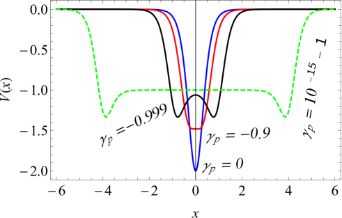
Figure 4: Potential profiles of (24) with different values of $\gamma_{p}$. Parameters used: $u_{0p}=1$, $g_{1p}=0.2$, $V_{0}=1$.

Interestingly, for $\gamma$ values deep in the flat-top regime, namely close to $-1$, the potential develops a two-well structure with minima located at $\pm\frac{1}{2}\,\sqrt{\frac{g_{1}}{u_{0}}}\,\ln\left[\frac{\sqrt{\gamma\,(8+17\gamma+9\gamma^{2})}}{2(1+\gamma)}-\frac{3\gamma}{2\sqrt{1+\gamma}}-\frac{1}{\sqrt{1+\gamma}}\right]$. The depth at the minima equals $u_{0}$, and the depth at the central peak is equal to $-3u_{0}/3\gamma$. This double-well potential, as we will see later, leads to reflectionless macroscopic quantum tunnelling.

In conclusion, a spectrum of solutions is obtained in terms of a single parameter, namely $\gamma$. A spectrum of reflectionless potentials is also obtained in terms of a single parameter, $\gamma_{p}$.

IV Resonant reflectionless scattering of flat-top and thin-top solitons

The purpose of this section is to confirm the reflectionless property of the potential derived in the previous section. This is performed through scattering of flat-top and thin-top solitons by the potential. In view of the fact that a spectrum of solutions and a corresponding spectrum of reflectionless potentials exist, we consider here possible combinations of solutions and potentials, as follows:

Bright soliton scattered by wide reflectionless potential well, $\gamma=0$, $\gamma_{p}=2\times 10^{-16}-1$:
This case shows an interesting resonant scattering of a bright soliton by a wide reflectionless potential where a multi-node trapped mode is formed. The sharp transition between full quantum reflection and full transmission is evident in Fig. 5.

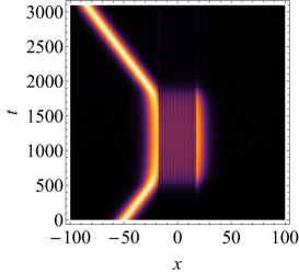
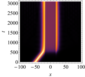
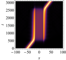
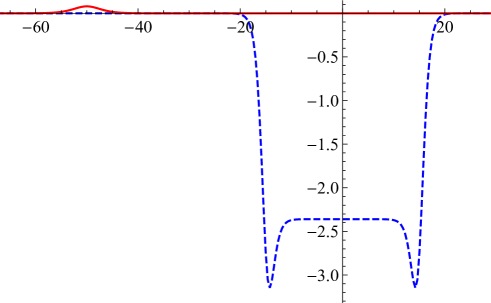
Figure 5: Resonant scattering of a bright soliton (3) by a wide reflectionless potential well, given by (24), with a varying potential well depth (a) $V_{0}=2.39417$, (b) $V_{0}=2.39418$, and (c) $V_{0}=2.39419$. The number of nodes in the formed trapped mode is 24 nodes. (d) Solution and potential profiles. The arrow shows the direction of motion for the incident soliton. Other parameters: $u_{0}=0.04$, $u_{0p}=0.2$, $\gamma=0$, $\gamma_{p}=-0.9999999999999998$, $v_{0}=0.05$, $g_{1}=0.5$, $g_{2}=1.0$, $g_{1p}=0.5$, $g_{2p}=1.0$.

It should be noted here that a square potential well with a similar width and depth would generate a considerable amount of radiation, which indicates the unique reflectionless feature of the potential at hand.

Flat-top soliton scattered by Pöschl-Teller potential well, $\gamma=-0.999999999999999$, $\gamma_{p}=0$:
It is interesting to see that such a huge soliton scatters coherently by the reflectionless potential. Quantum reflection and resonant scattering are clearly seen in Fig. 6.

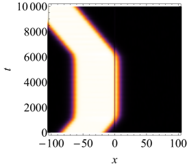
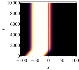
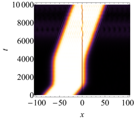
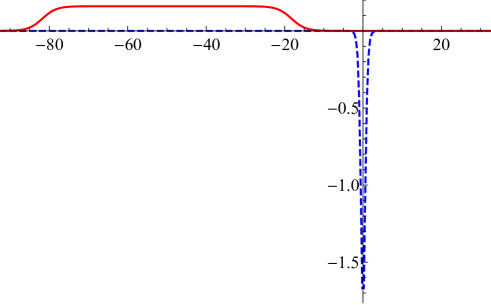
Figure 6: Resonant scattering of a flat-top soliton (7) by a Pöschl-Teller potential well (22) with a varying potential well depth (a) $V_{0}=0.895586$, (b) $V_{0}=0.8955860015377$, and (c) $V_{0}=0.895587$. (d) The solution and potential profiles. A single-node trapped mode is formed. The arrow shows the direction of motion for the incident soliton. Other parameters: $u_{0}=0.04$, $u_{0p}=2.44779$, $\gamma=-0.999999999999999$, $\gamma_{p}=0$, $v_{0}=0.017$, $g_{1}=0.5$, $g_{2}=1.0$, $g_{1p}=0.5$, $g_{2p}=1.0$.

It is known that a Pöschl-Teller potential with large modified width supports multi-node trapped modes, but loses its reflectionless property. In the present case, we report a situation where a potential with such a large width still results in a reflectionless scattering.

Flat-top soliton scattered by wide reflectionless potential well, macroscopic quantum tunnelling, $\gamma=\gamma_{p}=-0.998$:
This is a typical general case where a wide flat-top soliton is scattered by a wide reflectionless potential. Figure 7 shows reflectionless scattering together with multinode trapped modes excitation. It is interesting to see that with such a double-potential well, macroscopic quantum tunnelling occurs through the barrier between the two wells. This is similar to same phenomenon in Bose-Einstein condensates smerzi .

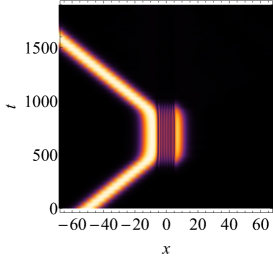
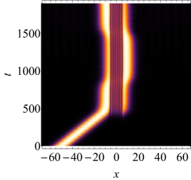
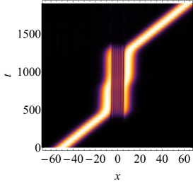
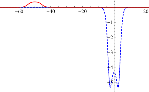
Figure 7: Resonant scattering of a flat-top soliton (7) by a wide reflectionless potential well with a varying potential well depth (a) $V_{0}=4.0$, (b) $V_{0}=4.00002762$, and (c) $V_{0}=4.000029$. (d) The solution and potential profiles. The number of nodes in the formed trapped mode is 10 nodes. The arrow shows the direction of motion for the incident soliton. Other parameters: $u_{0}=0.093748$, $u_{0p}=0.2$, $\gamma=\gamma_{p}=-0.998$, $v_{0}=0.1$, $g_{1}=0.5$, $g_{2}=1.0$, $g_{1p}=0.5$, $g_{2p}=1.0$.

Thin-top scattering: In a similar manner as for the flat-top solitons, we performed a series of simulations of scattering of thin-top solitons by a Pöschl-Teller potential well, shown in Fig. 8, a thin reflectionless potential well shown in Fig. 9, and a wide reflectionless potential well shown in Fig. 10. Similar results are obtained as for flat-top solitons.

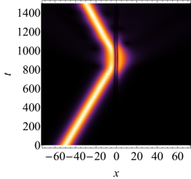
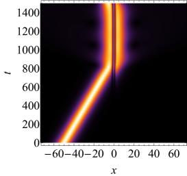
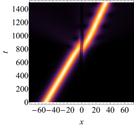
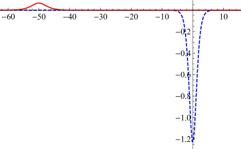
Figure 8: Resonant scattering of a thin-top soliton (8) by a Pöschl-Teller potential well with a varying potential well depth (a) $V_{0}=0.62$, (b) $V_{0}=0.621357995$, and (c) $V_{0}=0.635$. (d) The solution and potential profiles. A double-node trapped mode is formed. The arrow shows the direction of motion for the incident soliton. Other parameters: $u_{0}=0.04$, $u_{0p}=0.2$, $\gamma=1.0$, $\gamma_{p}=0$, $v_{0}=0.055$, $g_{1}=0.5$, $g_{2}=1.0$, $g_{1p}=0.5$, $g_{2p}=1.0$.

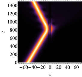
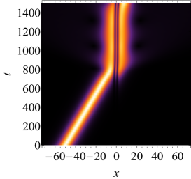
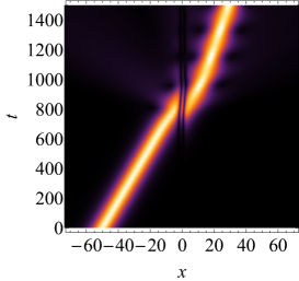
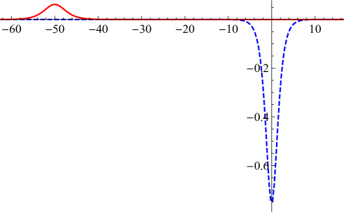
Figure 9: Resonant scattering of a thin-top soliton (8) by a thin reflectionless potential well with a varying potential well depth (a) $V_{0}=0.38$, (b) $V_{0}=0.3841987$, and (c) $V_{0}=0.395$. (d) The solution and potential profiles. A double-node trapped mode is formed. The arrow shows the direction of motion for the incident soliton. Other parameters: $u_{0}=0.04$, $u_{0p}=0.1$, $\gamma=\gamma_{p}=1.5$, $v_{0}=0.055$, $g_{1}=0.5$, $g_{2}=1.0$, $g_{1p}=0.5$, $g_{2p}=1.0$.

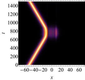
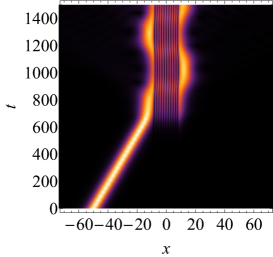
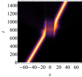
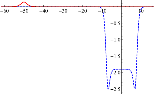
Figure 10: Resonant scattering of a thin-top soliton (8) by a wide reflectionless potential well with a varying potential well depth (a) $V_{0}=1.897$, (b) $V_{0}=1.898$, and (c) $V_{0}=1.9$. (d) The solution and potential profiles. The number of nodes in the formed trapped mode is 11 nodes. The arrow shows the direction of motion for the incident soliton. Other parameters: $u_{0}=0.0937480$, $u_{0p}=0.5$, $\gamma=1.5$, $\gamma_{p}=-0.9999999999$, $v_{0}=0.055$, $g_{1}=0.5$, $g_{2}=1.0$, $g_{1p}=0.7$, $g_{2p}=1.0$.

For further investigation of the resonant modes, we have studied the scattering of flat-top solitons by a wide reflectionless potential with varying depth. In terms of the potential depth, $V_{0}$, trapped modes with different numbers of nodes are excited. The associated resonant scattering occurs always when a trapped mode is excited. The number of nodes changes with the depth of the potential. As $V_{0}$ is increased, a trapped mode with an increasing number of nodes is found to occur at discrete values of $V_{0}$. This behavior is due to a resonance between the fixed energy of the incident soliton and the energy of the trapped modes. By increasing the magnitude of $V_{0}$, the energy of trapped modes increases and will resonate one after the other with the energy of the incident soliton. In Fig. 11, we plot the transport coefficients, reflectance $R=(1/n_{0})\int_{-\infty}^{-l}|\psi(x,\tau)|^{2}dx$, trapping $L=(1/n_{0})\int_{-l}^{l}|\psi(x,\tau)|^{2}dx$, and transmittance $T=(1/n_{0})\int_{-l}^{\infty}|\psi(x,\tau)|^{2}dx$, versus $V_{0}$. Here, $l$ is the length at which the potential is negligible and $\tau$ is a time long after the scattering event. The figure shows the multi-resonance behavior where three resonances are observed. It should be noted that a similar critical behavior in the transport coefficients may also be obtained by fixing the potential depth and varying the initial speed of the incident soliton. However, changing the potential depth leads to exciting many multi-nodes trapped modes, which is indicated by the multi-resonance behavior shown in Fig. 11. On the other hand, changing the soliton speed excites only one trapped mode at a certain critical speed.

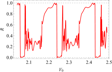
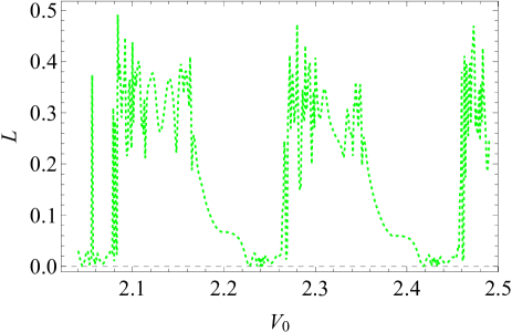
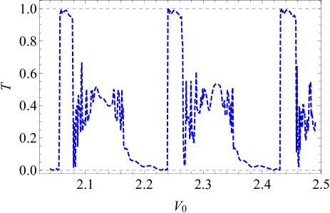
Figure 11: Scattering coefficients of (a) reflection, $R$, (b) trapping, $L$, and (c) transmission, $T$, for a flat-top soliton scattered by a wide reflectionless potential well with initial speed $v_{0}=0.1$. (d) A zoom-in of the three scattering coefficients for the left resonant scattering. Parameters used: $u_{0}=0.093748$, $u_{0p}=0.2$, $\gamma=-0.998$, $\gamma_{p}=-0.9999999999999998$, $g_{1}=0.5$, $g_{2}=1.0$, $g_{1p}=0.5$, $g_{2p}=1.0$.

Figure 12 shows the dynamics near resonances.

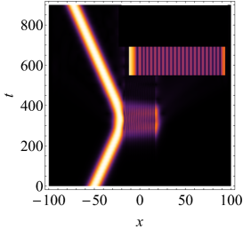
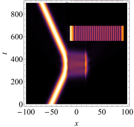
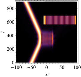
Figure 12: Full reflectance at resonances shown in Fig. 11(a) with a varying potential well depth (a) $V_{0}=2.046$ with a trapped mode of 22 nodes, (b) $V_{0}=2.236$ with a trapped mode of 23 nodes, and (c) $V_{0}=2.427$ with a trapped mode of 24 nodes. Insets show a zoom-in of the multi-node trapped modes. Other parameters: $u_{0}=0.093748$, $u_{0p}=0.2$, $\gamma=\gamma_{p}=-0.998$, $v_{0}=0.1$, $g_{1}=0.5$, $g_{2}=1.0$, $g_{1p}=0.5$, $g_{2p}=1.0$.

V Conclusions

From a generalized form of an exact solution to the NLSE with dual nonlinearity, we have shown that a spectrum of solutions exists containing four fundamentally different solutions, namely bright solitons, kink solitons, flat-top solitons, and thin-top solitons. We have shown that the four solutions are connected through one parameter that transfers one solution to the other.

Using a perturbative expansion with a trial solution corresponding to the scattered soliton, a general form of the reflectionless potential is obtained in terms of one of the solutions to the NLSE or any of its other integrable versions. Consequently, a spectrum of potentials is also obtained in terms of a single parameter.

A series of numerical simulations to the scattering of flat-top and thin-top solitons confirmed the reflectionless property of the potential. Resonant scattering and quantum reflection were generated in a similar manner as for the bright soliton scattering by a reflectionless Pöschl-Teller potential.

References

- (1) R. H. Goodman, P. J. Holmes, and M. I.Weinstein, Physica D 192, 215 (2004).
- (2) C. Lee and J. Brand, Europhys. Lett. 73, 321 (2006).
- (3) T. Ernst and J. Brand, Phys. Rev. A. 81, 033614 (2010).
- (4) L. Al Sakkaf and U. Al Khawaja, submitted (2022).
- (5) A. Hasegawa, Y. Kodama. Solitons in Optical Communications. New York: Oxford University Press; 1995. Mollenauer LF, and Gordon JP, Solitons in Optical Fibers (Acadamic Press, Boston, 2006); Agrawal GP, Nonlinear Fiber Optics (Academic Press, San Diego, 2001), 3rd ed.; Akhmediev NN, and Ankiexicz A, Solitons: Nonlinear Pulses and Beams (Chapman and Hall, London, 1997).
- (6) M. Asad-uz-zaman and U. Al Khawaja, Europhys. Lett. 101, 50008 (2013).
- (7) U. Al Khawaja, S. M. Al-Marzoug, H. Bahlouli, and Y. S. Kivshar, Phys. Rev. A 88, 023830 (2013).
- (8) U. Al Khawaja and A. A. Sukhorukov, Opt. Lett. 40, 2719 (2015).
- (9) C. R. Cabrera, et al., Science 359, 301 (2018).
- (10) P. Cheiney, et al., Phys. Rev. Lett. 120, 135301 (2018).
- (11) P. Cheiney, C.R. Cabrera, J. Sanz, B. Naylor, L. Tanzi, and L. Tarruell, Phys. Rev. Lett. 120, 135301 (2018).
- (12) F. Böttcher, J.N. Schmidt, J. Hertkorn, K.S. Ng, S.D. Graham, M. Guo, T. Langen, and T. Pfau, Rep. on Prog. in Phys. 84, 012403 (2020).
- (13) Z.H. Luo, W. Pang, B. Liu, Y.Y. Li, and B. A. Malomed, Front. of Phys. 16, 1 (2021).
- (14) A. Khare, S.M. Al-Marzoug, and H. Bahlouli, Phys. Lett. A 376, 2880 (2012).
- (15) U. Al Khawaja and H. Bahlouli, Comm. in Non. Sci. and Num. S. 69, 248 (2019).
- (16) A. Debnath, A. Khan, and S. Basu, Phys. Lett. A 439, 128137 (2022). .
- (17) D.S. Petrov, Phys. Rev. Lett. 115, 155302 (2015).
- (18) J. Chen and J. Zeng, Res. in Phys. 21, 103781 (2021).
- (19) M.R. Pathak and A. Nath, Sci. Rep. 12, 1 (2022).
- (20) L. Zeng and J. Zeng, JOSA B, 36, 2278 (2019).
- (21) B.A. Umarov,N.A.B. Aklan, M.R. Rosly, and T.H. Hassan, J. of Phys.: Conf. Ser. 890, 012071 (2017).
- (22) B.A. Umarov and N.A.B. Aklan, J. of Phys.: Conf. Ser. 819, 012023 (2017).
- (23) I. Kay and H.E. Moses, J. of App. Phys. 27, 1503 (1956).
- (24) L. Al Sakkaf and U. Al Khawaja, Alex. Eng. J. 61, 11803 (2022).
- (25) CJ. Pethick and H. Smith, Bose-Einstein Condensation in Dilute Gases. Cambridge: Cambridge University Press; 2001.
- (26) U. Al Khawaja and H. Bahlouli, CNSNS, 69, 248 (2019).
- (27) U. Al Khawaja, and L. Al Sakkaf, Handbook of Exact Solutions to the Nonlinear Schrödinger Equations, IOP Publishing Ltd 2020, London. Online ISBN: 978-0-7503-2428-1, Print ISBN: 978-0-7503-2426-7.
- (28) N.G. Vakhitov and A.A. Kolokolov, Radiophys. and Qua. Elect. 16, 783 (1973).
- (29) A. Smerzi, S. Fantoni, S. Giovanazzi, and S.R. Shenoy, Phys. Rev. Lett. 79, 4950 (1997).