Accurate Open-set Recognition for Memory Workload

Abstract.

How can we accurately identify new memory workloads while classifying known memory workloads? Verifying DRAM (Dynamic Random Access Memory) using various workloads is an important task to guarantee the quality of DRAM. A crucial component in the process is open-set recognition which aims to detect new workloads not seen in the training phase. Despite its importance, however, existing open-set recognition methods are unsatisfactory in terms of accuracy since they fail to exploit the characteristics of workload sequences.

In this paper, we propose Acorn, an accurate open-set recognition method capturing the characteristics of workload sequences. Acorn extracts two types of feature vectors to capture sequential patterns and spatial locality patterns in memory access. Acorn then uses the feature vectors to accurately classify a subsequence into one of the known classes or identify it as the unknown class. Experiments show that Acorn achieves state-of-the-art accuracy, giving up to $37\%$ points higher unknown class detection accuracy while achieving comparable known class classification accuracy than existing methods.

1. Introduction

How can we accurately identify new memory workloads while classifying known workloads? The global DRAM (Dynamic Random Access Memory) market size is about tens of billions USD, and keeps increasing due to growing demand of DRAM in mobile devices, modern computers, self-driving cars, etc. It is crucial to test DRAM using various workloads in verifying and guaranteeing DRAM quality. DRAM manufacturers utilize their known workloads for verification; however, it does not guarantee that DRAM works well for new workloads not known in advance. Therefore, it is necessary to detect new workloads to improve the quality of DRAM verification. The problem of detecting new workloads is formulated as an open-set recognition (Scheirer et al., 2013) task which classifies a test sample into the known classes or the unknown class, and identifies its class if it belongs to the known classes.

A workload sequence contains a series of tuples with the command and the address information of memory accesses. To detect new workloads based on open-set recognition, we exploit a subsequence, a part of the entire sequence of a workload. Given a subsequence, we classify it into one of the known workload classes or identify it as the unknown class corresponding to new workloads. Although there are several works (Bendale and Boult, 2016; Shu et al., 2017; Hassen and Chan, 2020; Liang et al., 2018; Lee et al., 2020) for the open-set recognition problem, none of them handles workload sequences. Their accuracy is limited for workload sequences since they do not exploit the characteristics of them. The major challenges to be tackled are 1) how to deal with very long subsequences (e.g., $100,000$), and 2) how to detect subsequences generated from new workloads not seen in the training phase.

We provide an example of how DRAM manufacturers use an open-set recognition method to improve DRAM verification. Executing a code generates a workload sequence which contains a series of tuples with the command and the address information of memory accesses. Assume that there is a code that frequently provokes memory failures, and there is a situation where we do not have the code but only have its workload sequence. Then, DRAM manufacturers want to design a test code similar to the failure-generating code since they need to verify DRAM for these failures. If an accurate open-set recognition method exists, the manufacturers utilize it to compare their code with failure-generating code, and design a new test code that generates failures. In addition, if a given sequence belongs to the unknown workload class, we train a new classifier with existing classes and the new class of the given sequence; then, we can precisely classify even the workload for the unknown class. This process helps prevent DRAM failures and improve DRAM quality. Therefore, we need to devise an accurate open-set recognition method for memory workload.

In this paper, we propose Acorn, an ACcurate Open-set recognition method for woRkload sequeNces, to classify a subsequence of a workload into known classes or identify it as the unknown class that has not been observed during training. To the best of our knowledge, Acorn is the first open-set recognition method for workload sequences. Acorn obtains feature vectors of subsequences by exploiting the characteristics of workload sequences. We split the workload fields into cmd and address-related fields, and extract features for each type. For the cmd field, we exploit $n$-gram models to capture sequential patterns and construct a feature vector using frequent $n$-grams. For the address-related fields, we construct a feature vector that captures the spatial locality patterns by counting the number of accesses to memory regions we carefully define. This process makes the proposed method extract representative patterns from the workloads. For the unknown class detection, we adopt the concept of anomaly detection based on a dimensionality reduction technique where abnormal test samples generate large reconstruction errors. Our main idea is to build an unknown class detector for each class using our feature vectors, to detect the pattern of the unknown class which deviates significantly from those of the known classes. It leads to accurate detection for test subsequences of the unknown class. Experimental results show that Acorn achieves the state-of-the-art performance in terms of both known class classification and unknown class detection, compared to baselines.

We summarize our main contributions as follows:

• Problem formulation and data. We formulate the new problem of open-set recognition for workload sequences (Problem 1), and release Memtest86-seq, the first public dataset containing a large-scale memory workload sequence generated from open-domain programs.

• Method. We propose Acorn, an effective and accurate method which extracts representative features from long workload subsequences and performs known class classification as well as unknown class detection.

• Experiment. Acorn outperforms existing open-set recognition methods by up to $37\%$ points higher unknown class detection accuracy with comparable known class accuracy than existing methods.

The rest of the paper is organized as follows: we give the related works and the problem definition in Section 2, propose Acorn in Section 3, show the experimental results in Section 4, and conclude in Section 5. The code and the dataset are available at https://github.com/snudatalab/Acorn.

2. Preliminaries

In this section, we describe the preliminaries and our problem definition. The notations used in this paper are given in Table 1.

Table 1. Symbols used in this paper.

Symbol	Description
$\mathbf{W}$	workload sequence matrix
$\mathbf{S}_{i}$	$i$-th subsequence matrix for training
$\mathcal{A}_{n}$	set of distinct n-grams
$|\boldsymbol{\mathcal{A}}_{n}|$	the cardinality of a set $\boldsymbol{\mathcal{A}}_{n}$
$\mathbf{x}_{i,CMD}$	the feature vector of cmd field for $i$-th training subsequence
$\mathbf{x}_{i,ADDRESS}$	the feature vector of address-related fields for $i$-th training subsequence
$\mathbf{V}_{w}$	unknown class detector matrix for a known class $w$
$\epsilon_{w}$	the threshold for a known class $w$

2.1. Workload Sequence

We use the term workload sequence to define a sequence of commands produced by a DRAM controller unit during the whole process of program execution.

Definition 0 (Workload Sequence).

A workload sequence $\mathbf{W}\in\mathbb{R}^{l\times 5}$ is a multidimensional sequence with the five fields cmd, rank, bank group, bank, and address, where $l$ is the length of the sequence.

• Command (cmd) - can be one of the following 5 commands: ACT, RDA, WRA, PRE, and PREA.

• Rank - rank number inside a DRAM.

• Bank Group - bank group number within a rank.

• Bank - bank number within a bank group.

• Address - corresponds to a row or column address within a bank.

Each row of a sequence consists of a command and $4$ address-related values. A value of the cmd field represents a type of operation or command. Address-related values for rank, bank group, bank, and address fields indicate the exact location in DRAM to which a command is applied.

DRAM Controller produces $25$ commands, and there are $5$ representative commands in the cmd field: ACT, RDA, WRA, PRE, and PREA. In a bank, ACT command is passed along with a row address to activate a row for the RDA or WRA command. When a row is activated, RDA or WRA commands can be transmitted along with a column number indicating column Read or Write followed by precharge operation. After all Read/Write operations to the activated row are completed, the PRE (precharge) command deactivates the row, so the next ACT command for a different row can be transmitted. Note that we cannot activate more than two rows at the same time in a bank. The PREA command deactivates all the active rows in all banks of a rank, so all the banks in the rank are ready to be accessed. We refer the reader to (ddr, 2013) for further details about the cmd field.

The values of address-related fields point out a specific location of a command operation. The rank is the highest level of organization which consists of several bank groups, and the bank group is a collection of banks. The value of the bank field is the index of a bank in the specified bank group. We can track the exact bank, which is a two-dimensional array whose cells store data, by combining the values of the rank, bank group, and bank fields since DRAM has a hierarchical structure. The address field of a workload sequence contains the information on the bank’s row number when the cmd field is ACT and a column number when the cmd field is either RDA or WRA. To detect the target memory cell where RDA/WRA command has been performed, one needs to find the preceding ACT command at the same rank, bank group, and bank. For example, Fig. 1 shows that write operation at location (2, 3) of rank 0, bank group 1, bank 1 since row number 2 was previously activated by the preceding ACT command with the same bank location.

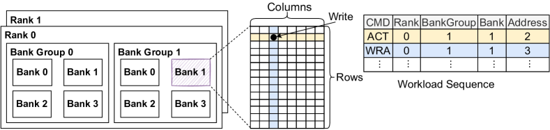
Figure 1. Workload sequence and address hierarchy in DRAM.

2.2. Open-set Recognition

Open-set recognition aims to detect samples from the unknown class not included in the training dataset, while classifying samples from known classes. Open-set recognition has been utilized for many real-world applications and is more challenging than semi-supervised learning (Yoo et al., 2019b; Chen et al., 2020; Luo et al., 2018) due to the unknown class detection. Zero-shot learning (Li et al., 2019; Yoo et al., 2019a) also identifies the unknown class, but it requires external knowledge which helps differentiate known and unknown classes. Since none of the existing methods take memory workloads as input, we describe previous model-agnostic methods that can be applied to open-set recognition for workload sequences. Model-agnostic methods can be combined with various deep learning-based models including MLP and CNN. Bendale et al. (Bendale and Boult, 2016) propose OpenMax layer which extends softmax for open-set recognition. Shu et al. (Shu et al., 2017) apply open-set recognition to sequence domain, introducing a document open classification (DOC) model that utilizes 1-vs-rest layer with a sigmoid function as an alternative to a softmax layer. Hassen et al. (Hassen and Chan, 2020) introduce ii-loss which forces a network to maximize the distance between given classes and minimize the distance between an instance and the center of its class in the feature space. Out-of-Distribution (OOD) methods (Liang et al., 2018; Lee et al., 2018; Lee et al., 2020; Liu et al., 2020; Sun et al., 2021) can be also applied to detect new workloads. Although the above methods have been applied to workload sequences, they fail to exploit the characteristics of the workload sequences. Yoshihashi et al. (Yoshihashi et al., 2019), Oza et al. (Oza and Patel, 2019), and Sun et al. (Sun et al., 2020) also address open-set recognition, but they require specific networks in contrast to the above methods.

2.3. Problem Definition

We use the term workload subsequence to define a sub-part of the workload which has been cut to the same length.

Definition 0 (Workload Subsequence).

Given a workload sequence matrix $\mathbf{W}\in\mathbb{R}^{l\times 5}$ where $l$ is the length of the sequence and $5$ is the number of the fields, a workload subsequence $\mathbf{S}^{(j)}\in\mathbb{R}^{l_{s}\times 5}$ is the $j$th vertical block matrix of $\mathbf{W}$ when $\mathbf{W}$ is vertically partitioned by length $l_{s}$ without overlapping: $\mathbf{W}=\begin{bmatrix}\mathbf{S}^{(1)}\\ \vdots\\ \mathbf{S}^{(l/l_{s})}\end{bmatrix}$. For simplicity, we represent a subsequence as $\mathbf{S}$ by dropping the notation $(j)$ describing the $j$th vertical block.

In this paper, we set the length $l_{s}$ of subsequences to $100,000$. We collect all subsequences $\mathbf{S}$ from all known workload sequences, and then randomly pick them to construct a set $\{(\mathbf{S}_{1},y_{1}),...,(\mathbf{S}_{N},y_{N})\}$ of training samples. $N$ is the number of training samples, $\mathbf{S}_{i}$ is the $i$th training subsequence, and $y_{i}$ is the label that indicates the workload that generated $\mathbf{S}_{i}$. The number of classes is equal to the number of known workloads when we train a model. Test samples consist of all subsequences for all unknown workloads and the subsequences not picked as the training samples for all known workloads.

We introduce the formal problem definition as follows:

Problem 1 (Workload Open-set Recognition).

Given a memory workload subsequence, classify it into one of the known classes or identify it as the unknown class.

• Known workloads are seen in the training phase, and a known workload corresponds to its known class.

• Unknown workloads are not seen in the training phase, and all unknown workloads correspond to the unknown class.

3. Proposed Method

In this section, we propose Acorn, an accurate open-set recognition method for workload sequences. We need to tackle the following challenges:

• Dealing with heterogeneous fields. How can we deal with $5$ heterogeneous fields, i.e., cmd, rank, bank group, bank, and address?

• Dealing with long subsequences for workload classification. It is impractical to train a classification model using workload subsequences whose length is $0.1$ million. How can we deal with long subsequences?

• Detecting new workloads unseen at the training phase. How can we identify unseen workloads that appear only in the test phase?

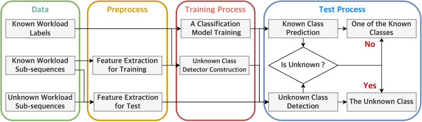
Figure 2. The overall process for Acorn on workload open-set recognition.

To achieve high accuracy for known class classification and unknown class detection, we propose the following main ideas:

• Discrimination-aware handling. The values of the cmd field and the address-related fields indicate the type of the operation and the location of the operation, respectively. We process the fields by considering the difference.

• Capturing sequential patterns and spatial locality patterns. We transform a long subsequence into two types of feature vectors of small sizes, and capture sequential and spatial patterns from the cmd and the address-related fields, respectively.

• Reconstruction error-based unknown class detection. Constructing an unknown class detector for each known class makes test subsequences of the unknown class have high reconstruction errors, clearly distinguishing them from those of the known classes.

Fig. 2 shows the overall process for Acorn. We construct training data with known workloads and test data using both known and unknown workloads. In the training process, we extract features from subsequences. Then, we train a classification model and construct unknown class detectors using the extracted features. In the test process, we find a feature vector of a test subsequence, predict a label $\hat{w}$ using the classification model, and then use a detector to identify whether it belongs to the label $\hat{w}$ or the unknown class.

3.1. Feature Extraction

The most important challenge is to effectively deal with a long subsequence with heterogeneous fields, while achieving high accuracy for workload classification. A naive approach is to train a classification model directly using subsequences. However, a subsequence $\mathbf{S}_{i}\in\mathbb{R}^{100,000\times 5}$ is too large to be used as an input for training a classification model. Moreover, the values in each field have different meanings. For example, $1$ in the cmd field indicates an ACT command while $1$ in the bank field indicates the second bank number in a bank group. Therefore, we need to extract a valuable feature vector from a subsequence. Our main ideas are to 1) separate the fields into two types, the cmd and the address-related fields (i.e., rank, bank group, bank, and address), and 2) consider the different characteristics of the two types in the fields.

CMD Feature Vector for Command Field. We first focus on transforming command lines $\mathbf{S}_{i}(:,0)\in\mathbb{R}^{100,000\times 1}$ of a subsequence into a feature vector of small size while capturing crucial information. Since each workload has a different order of occurring commands, capturing sequential patterns in the command lines is important; hence we exploit $n$-gram models, used in various applications (Tomovic et al., 2006; Zhang et al., 2019; Ali et al., 2020; Mutinda et al., 2021), which count a contiguous sequence of $n$ commands. We construct a set $\boldsymbol{\mathcal{A}}_{n}$ of $n$-gram sequences that frequently appear in workloads, and then transform command lines $\mathbf{S}_{i}(:,0)$ of a subsequence into a feature vector $\mathbf{c}_{i,n}\in\mathbb{R}^{|\boldsymbol{\mathcal{A}}_{n}|}$ using the set $\boldsymbol{\mathcal{A}}_{n}$ where $|\boldsymbol{\mathcal{A}}_{n}|$ is the cardinality of the set $\boldsymbol{\mathcal{A}}_{n}$. To be more specific, we count $n$-gram sequences from subsequences selected as training data for each workload, pick top-$m$ frequent $n$-gram sequences for each workload, and construct a set $\boldsymbol{\mathcal{A}}_{n}$ of the picked $n$-gram sequences collected from all known workloads. Then, for each $\mathbf{S}_{i}(:,0)$, we construct a feature vector $\mathbf{c}_{i,n}\in\mathbb{R}^{|\boldsymbol{\mathcal{A}}_{n}|}$ whose entry is the number of occurrences for its corresponding element in $\boldsymbol{\mathcal{A}}_{n}$. Fig. 3 shows an example of generating a feature vector of command lines.

To capture sequential patterns of diverse lengths, we use several $n$-gram models for different $n$s. In this paper, for each $\mathbf{S}_{i}(:,0)$, we use $7$, $11$ and $15$-gram models, generate three feature vectors $\mathbf{c}_{i,7}$, $\mathbf{c}_{i,11}$, and $\mathbf{c}_{i,15}$, and then construct a CMD feature vector $\mathbf{x}_{i,CMD}\in\mathbb{R}^{|\boldsymbol{\mathcal{A}}_{7}|+|\boldsymbol{\mathcal{A}}_{11}|+|\boldsymbol{\mathcal{A}}_{15}|}$ by concatenating $\mathbf{c}_{i,7}$, $\mathbf{c}_{i,11}$, and $\mathbf{c}_{i,15}$.

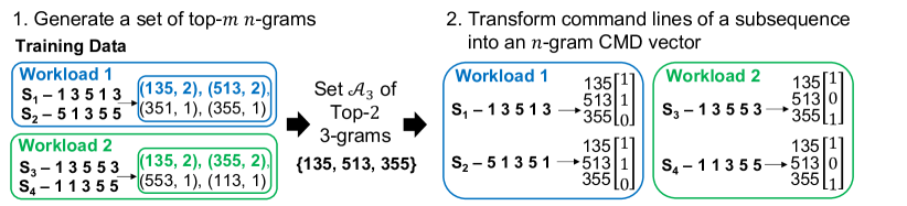
Figure 3. An example of generating a set of top-$m$ $n$-grams and an $n$-gram CMD vector of a subsequence. There are two workload sequences with $m=2$ and $n=3$.

ADDRESS Feature Vector for Address Related Fields. We next represent lines $\mathbf{S}_{i}$(:,1:4)$\in\mathbb{R}^{100,000\times 4}$ of address-related fields (i.e., rank, bank group, bank, and address) of a subsequence as a feature vector $\mathbf{x}_{i,ADDRESS}$ of a small size. In address-related fields, it is important to capture the access pattern in memory. Therefore, we count how many times addresses are accessed in a subsequence. A naive approach is to compute access counts for each cell. However, this generates a large feature vector whose size is equal to $(\textit{\# of rank})\times(\textit{\# of bank group})\times(\textit{\# of bank})\times(\textit{\# of address})$. To reduce the size of a feature vector for address-related fields, we separately model bank-level access and cell-level access. We also reduce the feature size for the cell-level access by defining memory regions and computing access counts for each region.

We first transform lines $\mathbf{S}_{i}$(:,1:3)$\in\mathbb{R}^{100,000\times 3}$ of the rank, bank group, and bank fields into a feature vector $\mathbf{b}_{i}$. Since there is a hierarchy for the three fields (see Fig. 1) where the bank field is the lowest level, we generate a bank counting feature vector $\mathbf{b}_{i}$ by computing access counts in $\mathbf{S}_{i}$(:,1:3) for each distinguished bank. For example, assume that there are $2$ ranks and each rank is a set of $4$ bank groups each of which has $4$ banks. The total number of distinct banks is $32=2\times 4\times 4$. Therefore, the size of a feature vector $\mathbf{b}_{i}$ is $32$, and an entry of the feature vector is the number of accesses for its corresponding bank.

We then transform address lines $\mathbf{S}_{i}(:,4)\in\mathbb{R}^{100,000\times 1}$ into a feature vector $\mathbf{d}_{i}$ of a small size. A naive approach is to construct a feature vector by counting the number of accesses to each cell. However, the size of this feature vector is equal to $(\textit{\# of distinct banks})\times\textit{size of a bank}$ (e.g., $32\times(2^{17}\times 2^{10})$). Therefore, we partition each 2D array into smaller block regions and count the number of accesses to each block region. A recent work (Zhang et al., 2022) segments memory address to solve the problem of its high granularity. Note that the difference between our address feature vector and the feature vector of the paper (Zhang et al., 2022) is the information that an address feature vector contains. Our address feature vector contains spatial information on the frequency of memory access in subsequence data, while the feature vector of the paper (Zhang et al., 2022) contains sequential information on the time of the memory access. For each distinct bank, we partition an address array of size $a_{r}\times a_{c}$ into $\frac{a_{r}}{g_{r}}\times\frac{a_{c}}{g_{c}}$ blocks of size $g_{r}\times g_{c}$, and generate a feature vector $\mathbf{d}_{i,b}\in\mathbb{R}^{\frac{a_{r}a_{c}}{g_{r}g_{c}}}$ by counting the number of accesses to blocks. We provide an example in Fig. 4. Then, we construct a feature vector $\mathbf{d}_{i}=\sum_{b=1}{\mathbf{d}_{i,b}}$ by summing up the feature vectors for all banks. We transform $\mathbf{S}_{i}$(:,1:4) into an ADDRESS feature vector $\mathbf{x}_{i,ADDRESS}=\left(\mathbf{b}_{i}\|\mathbf{d}_{i}\right)$.

In summary, we transform all subsequences $\mathbf{S}_{i}$ into feature vectors $\mathbf{x}_{i}$ by concatenating $\mathbf{x}_{i,CMD}$ and $\mathbf{x}_{i,ADDRESS}$, and exploit them for open-set recognition.

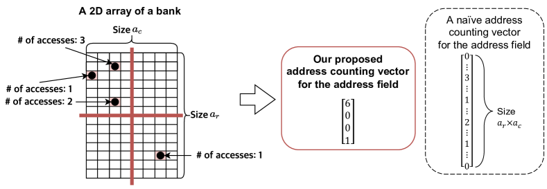
Figure 4. An example of constructing an address counting vector for the address field. We partition a 2D array into $4$ blocks by horizontal and vertical red lines, and then count the number of accesses in each block.

3.2. Classification Model and Unknown Class Detector

Training Classification Model. Given a set $\{(\mathbf{S}_{1},y_{1}),...,(\mathbf{S}_{N},y_{N})\}$ of training samples, our goal is to learn a classification model for known workloads. We construct a set $\{(\mathbf{x}_{1},y_{1}),...,(\mathbf{x}_{N},y_{N})\}$ by extracting feature vectors $\mathbf{x}_{i}$ from $\mathbf{S}_{i}$ for $i=1..N$, and then learn a classification model such as multi-layer perceptron.

Unknown Class Detectors. After training a model, we build detectors that accurately identify whether test samples are the unknown class or not. Given target size $R$ and a feature vector $\mathbf{x}^{\prime}\in\mathbb{R}^{F}$ of a test sample where $F$ is the size of $\mathbf{x}^{\prime}$, our strategy is to find a detector matrix $\mathbf{V}\in\mathbb{R}^{F\times R}$ based on training samples of known workloads, to measure a reconstruction error $\|\mathbf{x}^{\prime}-\mathbf{V}\mathbf{V}^{T}\mathbf{x}^{\prime}\|_{2}$. When $R$ is much smaller than $F$, the detector matrix maps a feature vector $\mathbf{x}^{\prime}$ to a lower dimension and remaps it to a higher dimension. The intuition is that test samples of known workloads generate low reconstruction errors while generating high reconstruction errors if test samples are from unknown workloads. A naive approach is to build one unknown workload detector for all known classes, but it fails to obtain a good decision boundary that distinguishes the unknown class from the known ones. Our main ideas are to 1) build unknown workload detectors $\mathbf{V}_{w}$ for each class $w$, and 2) exploit feature vectors of training samples. These ideas allow us to clearly distinguish test samples of known classes and the unknown class; the difference in reconstruction errors between them becomes high.

Our approach is to find a detector matrix $\mathbf{V}_{w}$ for a known class $w$, which identifies whether a test sample belongs to the unknown class or the known class $w$ based on the reconstruction error $\|\mathbf{x}^{\prime}-\mathbf{V}_{w}\mathbf{V}_{w}^{T}\mathbf{x}^{\prime}\|_{2}$. To obtain the matrix $\mathbf{V}_{w}$, we utilize Singular Value Decomposition (SVD) which is widely used in various applications including principal component analysis (PCA) (Jolliffe, 2002; Wall et al., 2003), data clustering (Simek et al., 2004; Osiński et al., 2004), tensor analysis (Jang and Kang, 2020), and time range analysis (Jang et al., 2018). With SVD, $\mathbf{V}_{w}$ minimizes the reconstruction error when a test sample $x^{\prime}$ belongs to the known class $w$. In contrast to the test samples of the known class $w$, a reconstruction error for a test sample of the unknown class is high since the characteristics of the known class $w$ are different from those of the unknown class. For each class $w$, we construct a matrix $\mathbf{X}_{w}\in\mathbb{R}^{N_{w}\times F}$ where each row corresponds to a feature vector of a training sample belonging to the class $w$. Note that $N_{w}$ is the number of training samples of the class $w$. Then, we perform SVD for the matrix $\mathbf{X}_{w}=\mathbf{U}_{w}\mathbf{\Sigma}_{w}\mathbf{V}_{w}^{T}$ and obtain the matrix $\mathbf{V}_{w}\in\mathbb{R}^{F\times R_{w}}$ of the right singular vectors where $R_{w}$ is target rank for the class $w$, to exploit it as a detector. With $\mathbf{V}_{w}$, we clearly identify whether a subsequence belongs to a known class $w$ or the unknown class by measuring a reconstruction error $\|\mathbf{x}^{\prime}-\mathbf{V}_{w}\mathbf{V}_{w}^{T}\mathbf{x}^{\prime}\|_{2}$. $\mathbf{x}^{\prime}$ is a feature vector of a test sample.

10:  A test sample $\mathbf{S}^{\prime}$, a trained classification model, a threshold hyperparameter $\alpha$,
unknown class detector matrices $\mathbf{V}_{w}\in\mathbb{R}^{F\times R_{w}}$, $\mu_{w}$, and $\sigma_{w}$ for $w=1,...,W$ where $W$ is the number of known classes

20:  One of the known class labels or the unknown class label for $\mathbf{S}^{\prime}$

1:  Feature Extraction. Transform $\mathbf{S}^{\prime}$ into a feature vector $\mathbf{x}^{\prime}\in\mathbb{R}^{F}$ using our feature
extraction approach in Section 3.1.

2:  Known Class Prediction. Predict a class label $\hat{w}$ using the trained classification model.

3:  Unknown Class Detection. Identify whether to satisfy $\|\mathbf{x}^{\prime}-\mathbf{V}_{\hat{w}}\mathbf{V}_{\hat{w}}^{T}\mathbf{x}^{\prime}\|_{2}<\mu_{\hat{w}}+\alpha*\sigma_{\hat{w}}$
for the $\hat{w}$th class. If the above inequality condition is satisfied, identify it as the predicted
class label $\hat{w}$. Otherwise, identify it as the unknown class label.

Algorithm 1 Acorn: Open-set Recognition for Workload Sequence

3.3. Open-set Recognition for Workload Sequence

We describe how to identify a test sample $\mathbf{S}^{\prime}$ as the unknown class using a trained classification model and SVD-based detectors (Algorithm 1). Given a feature vector $\mathbf{x}^{\prime}$ of the test sample, we first predict the class label $\hat{w}$ using the trained classification model where $\mathbf{x}^{\prime}$ is extracted from $\mathbf{S}^{\prime}$. After that, we recognize whether the test sample belongs to the predicted label or not by computing a reconstruction error with $\mathbf{V}_{\hat{w}}$. We recognize it as the predicted class label $\hat{w}$ only when the following inequality condition is satisfied.

(1) $$\|\mathbf{x}^{\prime}-\mathbf{V}_{\hat{w}}\mathbf{V}_{\hat{w}}^{T}\mathbf{x}^{\prime}\|_{2}<\epsilon_{\hat{w}}$$

where $\mathbf{V}_{\hat{w}}\mathbf{V}_{\hat{w}}^{T}\mathbf{x}^{\prime}$ is the reconstructed vector. When Eq. (1) is not satisfied, we determine that the test sample belongs to the unknown class. We set a threshold $\epsilon_{\hat{w}}$ to $\mu_{\hat{w}}+\alpha*\sigma_{\hat{w}}$ where $\mu_{\hat{w}}$ and $\sigma_{\hat{w}}$ are the mean and the standard deviation of reconstruction errors for feature vectors of training samples of the class $\hat{w}$, respectively. $\alpha$ provides a trade-off between known class classification accuracy and unknown class detection accuracy. A high $\alpha$ increases known class classification accuracy, but decreases unknown class detection accuracy. This is because false negatives increase while false positives decrease for the unknown class. A low $\alpha$ does the opposite.

4. Experiments

In this section, we experimentally evaluate the performance of Acorn. We aim to answer the following questions:

• Performance (Section 4.2). How accurately does Acorn classify subsequences from known workloads and detect subsequences from unknown workloads?

• Feature Effectiveness (Section 4.3). How successfully do our feature vectors improve the classification accuracy?

• Effectiveness of Per-Class Detector (Section 4.4). How accurately do per-class detectors identify the unknown class compared to the naive detector?

4.1. Experimental Setting

We construct our model using the Pytorch framework. All the models are trained and tested on a machine with a GeForce GTX 1080 Ti GPU.

Datasets. We use two real-world workload sequence datasets summarized in Table 2. There are $44$ and $34$ workloads for SEC-seq and Memtest86-seq, respectively. We publicize Memtest86-seq dataset which is generated from an open-source software program for DRAM test. Memtest86 uses two different algorithms to find out memory errors which are often caused by interaction between memory cells. For a workload, we collect signals using an equipment capturing DRAM signal, and transform the signals into a sequence with $5$ heterogeneous fields in Definition 1. The lengths of each workload sequence are different.

DRAM Specification. Both SEC-seq and Memtest86-seq datasets are generated on a server with Samsung 32GB 2Rx4 2666Mhz DRAM chip and Intel Gold6248 CPU. The DRAM chip has 2 ranks, and there are $4$ bank groups in a rank and $4$ banks in a bank group so that there are $2\times 4\times 4=32$ distinct banks. Each bank has $2^{17}$ rows and $2^{10}$ columns with a cell size of $8$ Bytes which gives total of $2^{17}\times 2^{10}\times 8$ Bytes = $1$GB.

Table 2. Datasets. known and unknown are the short term for known workloads and unknown workloads, respectively. The number of known workloads is equal to the number of known classes. All unknown workloads correspond to one unknown class.

	# of known	# of unknown	# of	# of test	# of test
Dataset	workloads	workloads	train	of known	of unknown
SEC-seq3	$40$	$4$	$586,885$	$293,444$	$93,491$
Memtest86-seq4	$31$	$3$	$433,334$	$216,696$	$77,018$

Competitors for open-set recognition. We compare Acorn with the following $9$ competitors for open-set recognition:

• Naive Rejection (Hendrycks and Gimpel, 2017) identifies a test sample as the unknown class when the maximum softmax score of a trained model is below a threshold.

• OpenMax (Bendale and Boult, 2016) adds a new class called unknown and applies softmax with a threshold.

• ii-loss (Hassen and Chan, 2020) forces a network to maximize the distances between known classes and minimize the distance between an instance and the center of its class.

• DOC (Shu et al., 2017) changes the softmax layer to 1-vs.-rest layer with sigmoid function.

• ODIN (Liang et al., 2018) adds a small perturbation to the input and divides softmax values by temperature parameter $T$.

• Mahalanobis-based detector (Lee et al., 2018) computes the confidence score using Mahalanobis distance instead of Euclidean distance.

• Deep-MCDD (Lee et al., 2020) obtains spherical decision boundary for each given class and computes the distances of samples from each class.

• Energy-based detector (Liu et al., 2020) uses energy scores to differentiate the out-of-distribution data from the in-distribution data.

• ReAct (Sun et al., 2021) applies rectified activation on the penultimate layer of a network and calculates the confidence score.

We use $2$-layer MLP as a classification model, and all the methods are combined with the MLP. In addition, Acorn and competitors use the same input feature vectors. This is because it is impracticable for using a subsequence of size $100,000\times 5$ not processed by our feature extraction method to learn competitors. Our feature extraction method enables us to learn models effectively on our open-set recognition task.

Hyperparameter Settings. We use the following hyperparameters in experiments:

• Hyperparameters for $n$-gram CMD vectors.

  • We construct three $n$-gram CMD vectors for each subsequence: $n=7,11,$ and $15$.

  • In order to generate a set $\boldsymbol{\mathcal{A}}_{n}$, we select top-$m$ $n$-gram CMD vectors for each $n$ with $m=25$.

  • For SEC-seq, $|\boldsymbol{\mathcal{A}}_{7}|$, $|\boldsymbol{\mathcal{A}}_{11}|$, and $|\boldsymbol{\mathcal{A}}_{15}|$ are $154$, $236$, and $289$, respectively. For Memtest86-seq, $|\boldsymbol{\mathcal{A}}_{7}|$, $|\boldsymbol{\mathcal{A}}_{11}|$, and $|\boldsymbol{\mathcal{A}}_{15}|$ are $132$, $196$, and $215$, respectively.

• Hyperparameters for address counting vectors.

  • We split an address array of size $2^{17}\times 2^{10}$ into $8\times 128$ blocks of size $2^{14}\times 8$ where $g_{r}$ and $g_{c}$ are equal to $2^{14}$ and $8$, respectively.

• Hyperparameters for our open-set recognition model.

  • For multi-layer perceptron (MLP), we use Adam optimizer with a learning rate of $0.0001$ and fix the batch size to $128$.

  • The total number of epochs is set to $5$.

  • We set $\alpha$ as one of $\{1,1.5,2,2.5,3\}$ to compute the threshold of Acorn, and select thresholds of the competitors based on their papers.

  • The rank $R_{w}$ is set to the minimum value $r$ that satisfies $\sum_{k=1}^{r}{\lambda^{2}_{k}}>0.999\times\sum_{k=1}^{\min{(N_{w},F)}}{\lambda^{2}_{k}}$ for a class $w$ where $\lambda_{k}$ is the $k$th singular value of the SVD result for $\mathbf{X}_{w}$.

Evaluation Metrics. Accuracy $(\%)$ for known classes is equal to $(\bar{N}^{\prime}_{known}/N^{\prime}_{known})\times 100$ where $N^{\prime}_{known}$ is the number of test samples of known classes and $\bar{N}^{\prime}_{known}$ is the number of test samples correctly classified as true known classes. The metrics of precision $(\%)$ and recall $(\%)$ for the unknown class are also used for unknown class detection. We compute f1-score $(\%)$ to show the trade-off between the unknown class recall and unknown class precision.

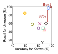
(a) SEC-seq

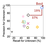
(b) SEC-seq

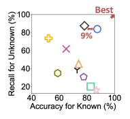
(c) Memtest86-seq

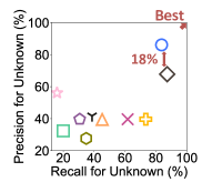
(d) Memtest86-seq

Figure 5. Performance for open-set recognition. Note that the best results of each method are reported. Acorn provides the best trade-off between accuracy for known class classification and precision & recall for unknown class detection.

4.2. Performance

In this section, we show the performance of Acorn in terms of known class classification accuracy, unknown class recall, unknown class precision, and inference time.

4.2.1. Accuracy

We compare the performance of Acorn with competitors on the open-set recognition task. We observe known class classification accuracy, unknown class recall, and unknown class precision. We report F1-score for unknown class detection to show the trade-off between the precision and recall. Fig. 5 visualizes the best trade-off between the evaluation metrics of the proposed method and the competitive methods. For both datasets, Acorn provides the best performance compared to various open-set recognition methods. In Fig. 5(a) and  5(b), Acorn achieves $37\%$ points higher recall and $19\%$ points higher precision for the unknown class than the second-best competitor Deep-MCDD. In Fig. 5(c) and  5(d), Acorn gives $9\%$ points higher known class classification accuracy and $18\%$ points higher precision for the unknown class than the second-best method while having a similar recall. We also report the overall results of the proposed method and the competitors for both datasets in Table 3. As for ii-loss method, the best known class accuracy is lower than $95\%$ points and $90\%$ points for SEC-seq and Memtest86-seq datasets, respectively; thus, we do not report the performance for these cases. Acorn shows the highest unknown class f1-score with fixed known class accuracy for all cases. The performance gap occurs since Acorn constructs an unknown class detector by exploiting feature vectors, while competitors use hidden vectors generated from known classification models. The hidden vectors do not contain enough information to detect the unknown class since known classification models concentrate only on extracting information that classifies an input into known ones.

Table 3. Performance for the open-set recognition. acc., rec., prec., and f1 denote known class accuracy, unknown class recall, unknown class precision, and unknown class f1-score, respectively. Bold and underlined text represent the best and the second-best performance, respectively.

Method	SEC-seq						Memtest86-seq
	acc. = 95			acc. = 85			acc. = 90			acc. = 80
	rec.	prec.	f1	rec.	prec.	f1	rec.	prec.	f1	rec.	prec.	f1
Naive Rejection	19.66	64.53	30.14	48.92	54.41	51.52	16.81	60.35	26.30	44.13	46.42	45.25
OpenMax	29.02	82.73	42.97	48.97	52.90	50.86	12.35	58.07	20.37	25.70	32.92	28.87
ii-loss	—	—	—	14.19	36.97	20.51	—	—	—	18.78	50.72	27.41
DOC	23.10	84.19	36.25	58.18	58.24	58.21	3.17	86.19	6.12	24.22	35.35	28.75
ODIN	16.56	75.16	27.14	50.17	55.49	52.70	8.06	70.29	14.46	12.04	24.75	16.20
Mahalanobis	5.74	28.72	9.57	11.62	19.72	14.62	3.14	27.71	5.64	13.41	19.91	16.03
Deep-MCDD	19.28	94.96	32.05	61.13	73.26	66.65	16.39	90.09	27.74	83.23	70.49	76.33
Energy	23.21	78.54	35.83	59.44	71.48	64.91	9.01	51.63	15.34	19.08	43.59	26.54
ReAct	16.94	75.98	27.70	17.59	38.99	24.24	7.27	61.83	13.01	7.36	20.53	10.84
Acorn	97.05	93.96	95.48	99.88	73.15	84.45	60.33	91.71	72.78	95.11	72.41	82.22

4.2.2. Inference time

We compare the inference time of the proposed method with competitors in Table 4. We measure the CPU running time of the inference procedure. Acorn takes the second shortest inference times which are $46.47$ and $24.03$ seconds slower than DOC for SEC-seq and Memtest86-seq datasets, respectively. However, the proposed method shows better performance than DOC for all cases. Acorn achieves $59.23\%$ points higher unknown class f1-score than DOC when the known class accuracy is fixed as $95\%$ points. For Memtest86-seq, Acorn achieves $66.66\%$ points higher f1-score than DOC, while having the same accuracy. Acorn is the only method to achieve high accuracy and fast inference simultaneously on the workload open-set recognition task.

Table 4. Performance for the inference time. Naive, Mahal., and MCDD are abbreviations for Naive Rejection, Mahalanobis, and Deep-MCDD methods, respectively. We report the fastest time as bold and the second fastest time as underline.

Dataset	Naive	OpenMax	ii-loss	DOC	ODIN	Mahal.	MCDD	Energy	ReAct	Acorn
SEC-seq	250.60	548.35	225.23	29.68	80.65	2852.02	635.80	773.28	1731.35	76.15
Memtest86-seq	155.25	372.16	138.18	31.94	77.98	1109.93	378.44	539.98	1608.12	55.97

4.3. Feature Effectiveness

We evaluate models for 6 different feature vectors: CMD (only $7$-gram), CMD (only $11$-gram), CMD (only $15$-gram), CMD (the concatenation of $7,11$, and $15$-grams CMD vectors), ADDRESS, and CMD + ADDRESS (the concatenation of the $7,11$, and $15$-grams CMD vectors, and the ADDRESS vector). We evaluate classification accuracy for known classes. Table 5 shows the results for both datasets. Our CMD + ADDRESS feature vectors make the model (MLP) achieve the highest classification accuracy. For both datasets, ADDRESS feature vectors are more effective than CMD vectors, since ADDRESS vectors give more detailed information on the target address than CMD vectors do. In addition, using several $n$-gram models provides higher accuracy than using one $n$-gram model.

Table 5. Feature effectiveness. Our feature vectors (CMD + ADDRESS) make the classifier model (MLP) achieve the highest accuracy for known classes.

	CMD	CMD	CMD			CMD +
Dataset	(only 7-gram)	(only 11-gram)	(only 15-gram)	CMD	ADDRESS	ADDRESS
SEC-seq	$82.20\%$	$81.92\%$	$80.13\%$	$83.56\%$	$90.88\%$	$\mathbf{97.02\%}$
Memtest86-seq	$65.93\%$	$62.68\%$	$57.54\%$	$67.42\%$	$76.29\%$	$\mathbf{92.08\%}$

Table 6. Comparison between the naive method and Acorn for unknown workload detection. $\alpha$ is a hyperparameter for thresholds. Note that acc., rec., and prec. denote known class accuracy, unknown class recall, and unknown class precision, respectively. See Section 4.4 for details.

SEC-seq	$\alpha$ = 1			$\alpha$ = 1.5			$\alpha$ = 2			$\alpha$ = 2.5			$\alpha$ = 3
	acc.	rec.	prec.	acc.	rec.	prec.	acc.	rec.	prec.	acc.	rec.	prec.	acc.	rec.	prec.
Naïve	81.80	47.27	51.23	87.23	29.44	50.59	91.44	19.41	54.34	94.20	12.10	59.65	95.74	7.95	68.32
Acorn	86.19	99.86	75.35	90.79	99.5	83.97	93.04	98.83	89.00	94.27	98.04	92.05	$\mathbf{95.00}$	$\mathbf{97.05}$	$\mathbf{93.96}$

Memtest86-seq	$\alpha$ = 1			$\alpha$ = 1.5			$\alpha$ = 2			$\alpha$ = 2.5			$\alpha$ = 3
	acc.	rec.	prec.	acc.	rec.	prec.	acc.	rec.	prec.	acc.	rec.	prec.	acc.	rec.	prec.
Naïve	76.99	78.78	64.21	83.68	70.76	74.62	88.62	60.37	86.60	90.64	49.14	93.67	91.25	39.85	96.18
Acorn	83.12	92.25	77.67	$\mathbf{87.52}$	$\mathbf{83.70}$	$\mathbf{86.12}$	89.36	72.57	90.04	90.22	60.33	91.71	90.67	48.23	92.21

4.4. Effectiveness of Per Class Detector

We compare Acorn and the naive SVD detector that does not consider classes.

• Naive: we obtain one $\mathbf{V}$ by computing SVD for all training samples, and then recognize a test sample using $\mathbf{V}$ by computing a reconstruction error.

Table 6 shows that Acorn achieves much higher performance than the naive SVD detector. For SEC-seq, Acorn outperforms the naive detector for all $\alpha$. At $\alpha=3$, Acorn gives $89\%$ points higher recall and $25\%$ points higher precision than the naive one while having a comparable known class accuracy. For Memtest86-seq, Acorn and the naive detector have comparable known class accuracies and precision, but Acorn gives at least $8.3\%$ points higher recall than the naive one. Since feature vectors of classes have different patterns, the single $\mathbf{V}$ of the naive method fails to have the capacity to distinguish known classes and the unknown class.

5. Conclusion

In this paper, we propose Acorn, an accurate open-set recognition method for workload sequences. Acorn extracts an effective feature vector of a small size from a subsequence by exploiting the characteristics of workload sequences. Based on the feature vectors, Acorn accurately detects test samples of the unknown class by constructing SVD-based detectors for each class. Experiments show that Acorn outperforms existing open-set recognition methods, simultaneously achieving higher performance for known classes and the unknown class. Future works include a novel feature extraction method considering the association between heterogeneous fields, and extending the proposed method for other applications such as malware detection.

- (1)
- ddr (2013) 2013. SDRAM STANDARD. (2013). https://www.jedec.org/sites/default/files/docs/JESD79-4.pdf
- Ali et al. (2020) Muhammad Ali, Stavros Shiaeles, Gueltoum Bendiab, and Bogdan Ghita. 2020. MALGRA: Machine learning and N-gram malware feature extraction and detection system. Electronics 9, 11 (2020), 1777.
- Bendale and Boult (2016) Abhijit Bendale and Terrance E. Boult. 2016. Towards Open Set Deep Networks. In CVPR. IEEE Computer Society, 1563–1572.
- Chen et al. (2020) Kaixuan Chen, Lina Yao, Dalin Zhang, Xianzhi Wang, Xiaojun Chang, and Feiping Nie. 2020. A Semisupervised Recurrent Convolutional Attention Model for Human Activity Recognition. IEEE Trans. Neural Networks Learn. Syst. 31, 5 (2020), 1747–1756.
- Hassen and Chan (2020) Mehadi Hassen and Philip K. Chan. 2020. Learning a Neural-network-based Representation for Open Set Recognition. In SDM. SIAM, 154–162.
- Hendrycks and Gimpel (2017) Dan Hendrycks and Kevin Gimpel. 2017. A Baseline for Detecting Misclassified and Out-of-Distribution Examples in Neural Networks. In 5th International Conference on Learning Representations, ICLR 2017, Toulon, France, April 24-26, 2017, Conference Track Proceedings. OpenReview.net.
- Jang et al. (2018) Jun-Gi Jang, Dongjin Choi, Jinhong Jung, and U Kang. 2018. Zoom-SVD: Fast and Memory Efficient Method for Extracting Key Patterns in an Arbitrary Time Range. In CIKM. ACM, 1083–1092.
- Jang and Kang (2020) Jun-Gi Jang and U Kang. 2020. D-Tucker: Fast and Memory-Efficient Tucker Decomposition for Dense Tensors. In ICDE. IEEE, 1850–1853.
- Jolliffe (2002) Ian Jolliffe. 2002. Principal component analysis. Wiley Online Library.
- Lee et al. (2020) Dongha Lee, Sehun Yu, and Hwanjo Yu. 2020. Multi-Class Data Description for Out-of-distribution Detection. In KDD. ACM, 1362–1370.
- Lee et al. (2018) Kimin Lee, Kibok Lee, Honglak Lee, and Jinwoo Shin. 2018. A Simple Unified Framework for Detecting Out-of-Distribution Samples and Adversarial Attacks. In NeurIPS 2018. 7167–7177.
- Li et al. (2019) Zhihui Li, Lina Yao, Xiaojun Chang, Kun Zhan, Jiande Sun, and Huaxiang Zhang. 2019. Zero-shot event detection via event-adaptive concept relevance mining. Pattern Recognit. 88 (2019), 595–603.
- Liang et al. (2018) Shiyu Liang, Yixuan Li, and R. Srikant. 2018. Enhancing The Reliability of Out-of-distribution Image Detection in Neural Networks. In ICLR. OpenReview.net.
- Liu et al. (2020) Weitang Liu, Xiaoyun Wang, John D. Owens, and Yixuan Li. 2020. Energy-based Out-of-distribution Detection. In NeurIPS.
- Luo et al. (2018) Minnan Luo, Xiaojun Chang, Liqiang Nie, Yi Yang, Alexander G. Hauptmann, and Qinghua Zheng. 2018. An Adaptive Semisupervised Feature Analysis for Video Semantic Recognition. IEEE Trans. Cybern. 48, 2 (2018), 648–660.
- Mutinda et al. (2021) James Mutinda, Waweru Mwangi, and George Okeyo. 2021. Lexicon-pointed hybrid N-gram Features Extraction Model (LeNFEM) for sentence level sentiment analysis. Engineering Reports 3, 8 (2021), e12374.
- Osiński et al. (2004) Stanisław Osiński, Jerzy Stefanowski, and Dawid Weiss. 2004. Lingo: Search results clustering algorithm based on singular value decomposition. In Intelligent information processing and web mining. Springer, 359–368.
- Oza and Patel (2019) Poojan Oza and Vishal M. Patel. 2019. C2AE: Class Conditioned Auto-Encoder for Open-Set Recognition. In CVPR. Computer Vision Foundation / IEEE, 2307–2316.
- Scheirer et al. (2013) Walter J. Scheirer, Anderson de Rezende Rocha, Archana Sapkota, and Terrance E. Boult. 2013. Toward Open Set Recognition. IEEE Trans. Pattern Anal. Mach. Intell. 35, 7 (2013), 1757–1772.
- Shu et al. (2017) Lei Shu, Hu Xu, and Bing Liu. 2017. DOC: Deep Open Classification of Text Documents. In EMNLP. Association for Computational Linguistics, 2911–2916.
- Simek et al. (2004) Krzysztof Simek, Krzysztof Fujarewicz, Andrzej Świerniak, Marek Kimmel, Barbara Jarzab, Małgorzata Wiench, and Joanna Rzeszowska. 2004. Using SVD and SVM methods for selection, classification, clustering and modeling of DNA microarray data. Engineering Applications of Artificial Intelligence 17, 4 (2004), 417–427.
- Sun et al. (2020) Xin Sun, Zhenning Yang, Chi Zhang, Keck Voon Ling, and Guohao Peng. 2020. Conditional Gaussian Distribution Learning for Open Set Recognition. In CVPR. IEEE, 13477–13486.
- Sun et al. (2021) Yiyou Sun, Chuan Guo, and Yixuan Li. 2021. ReAct: Out-of-distribution Detection With Rectified Activations. Advances in Neural Information Processing Systems (2021).
- Tomovic et al. (2006) Andrija Tomovic, Predrag Janicic, and Vlado Keselj. 2006. n-Gram-based classification and unsupervised hierarchical clustering of genome sequences. Comput. Methods Programs Biomed. 81, 2 (2006), 137–153.
- Wall et al. (2003) Michael E Wall, Andreas Rechtsteiner, and Luis M Rocha. 2003. Singular value decomposition and principal component analysis. In A practical approach to microarray data analysis. Springer, 91–109.
- Yoo et al. (2019a) Jaemin Yoo, Minyong Cho, Taebum Kim, and U Kang. 2019a. Knowledge Extraction with No Observable Data. In NeurIPS. 2701–2710.
- Yoo et al. (2019b) Jaemin Yoo, Hyunsik Jeon, and U Kang. 2019b. Belief Propagation Network for Hard Inductive Semi-Supervised Learning. In IJCAI, Sarit Kraus (Ed.). ijcai.org, 4178–4184.
- Yoshihashi et al. (2019) Ryota Yoshihashi, Wen Shao, Rei Kawakami, Shaodi You, Makoto Iida, and Takeshi Naemura. 2019. Classification-Reconstruction Learning for Open-Set Recognition. In CVPR. Computer Vision Foundation / IEEE, 4016–4025.
- Zhang et al. (2019) Hanqi Zhang, Xi Xiao, Francesco Mercaldo, Shiguang Ni, Fabio Martinelli, and Arun Kumar Sangaiah. 2019. Classification of ransomware families with machine learning based on N-gram of opcodes. Future Gener. Comput. Syst. 90 (2019), 211–221.
- Zhang et al. (2022) Pengmiao Zhang, Ajitesh Srivastava, Anant V. Nori, Rajgopal Kannan, and Viktor K. Prasanna. 2022. Fine-grained address segmentation for attention-based variable-degree prefetching. In CF ’22: 19th ACM International Conference on Computing Frontiers, Turin, Italy, May 17 - 22, 2022. ACM, 103–112.