FSCNN: A Fast Sparse Convolution Neural Network Inference System

Abstract

Convolution neural networks (CNNs) have achieved remarkable success, but typically accompany high computation cost and numerous redundant weight parameters. To reduce the FLOPs, structure pruning is a popular approach to remove the entire hidden structures via introducing coarse-grained sparsity. Meanwhile, plentiful pruning works leverage fine-grained sparsity instead (sparsity are randomly distributed), whereas their sparse models lack special designed computing library for potential speedup. In this technical report, we study and present an efficient convolution neural network inference system to accelerate its forward pass by utilizing the fine-grained sparsity of compressed CNNs. Our developed FSCNN is established based on a set of specialized designed sparse data structures, operators and associated algorithms. Experimentally, we validate that FSCNN outperforms standard deep learning library PyTorch on popular CNN architectures such as VGG16 if sufficiently high sparsity exhibits. However, due to the contiguity issue of sparse operators, FSCNN is typically not comparable with highly optimized dense operator. Therefore, coarse-grained (structured) sparsity is our recommendation for generic model compression.

1 Introduction

Convolutional Neural Network (CNN) has demonstrated its success in plentiful computer vision application [21, 11, 28]. However, the structure of CNN typically results in high computational cost during inference, which encumbers its deployment into mobile devices [22]. To address this issue, extensive works have been done on accelerating neural networks by compression [13, 18, 15, 7], quantization [26], tensor factorization [18] and special convolution implementations [8, 16, 31].

As a common practice, model compression is achieved by reducing the number of parameters and computation of each layer in deep neural networks. It can be largely evolved into two categories: (i) fine-grained pruning and (ii) structured pruning [2]. Fine-grained pruning aims to prune individual unimportant elements in weight tensors to zeros, which achieves very high sparse weights with no loss of accuracy [14]. To achieve sparse weights, sparsity-inducing regularized optimization, e.g. $\ell_{1}$-regularization, is the common technique that has been demonstrated to yield extremely high sparse solution with satisfying model accuracy effectively [23]. More specifically, some state-of-the-art stochastic $\ell_{1}$-regularized solvers [20] are able to compute model weights with sparsity higher than 95% without sacrificing generalization performance on testing data.

However, such sparsity-inducing techniques result in an irregular pattern of sparsity, and require specialized hardware system such as [12, 6] for speed up. Recent specialized inference systems are typically established by extending well-known Compressed Sparse Row(Column) (CSR(C)) format [29] for sparse matrices, and using sparse operations in varying ways. For examples, EIE [12] accelerates the fully connected layers of CNN. Sparse CNN [23] decomposes the convolutional filters approximately into a set of sparse matrices, (referred as DSCNN throughout this paper). Escoin [6] constructs a sequence of sparse matrix multiplications to form convolutional operations on GPUs.

We have the perspective that EIE, DSCNN and Escoin are valuable state-of-the-art sparse inference systems of CNN with visible advantages and disadvantages. Particularly, EIE partially employs sparse operators into CNN, i.e., the fully connected layers, rather than the dominate convolutional layers. DSCNN approximates the convolutional filters into sparse matrix multiplications which may result in sacrificing precision of inference. Escoin on the other hand, implements the exact sparse convolution by stacking sparse matrix multiplications, but focuses on GPUs, while in the recent world CPUs are still the major inference platform, and GPUs appear more during training stage [22].

In this paper, we propose, develop, analyze, and provide numerical results for a new sparse convolutional neural network inference accelerator for CPUs, named as Fast Sparse Convolutional Neural Network (FSCNN). As an overview, our FSCNN considers two types of sparsity, i.e., either filters or input tensors of convolutional layers are sparse, tackled by two variants Sparse Filter CNN and Sparse Input CNN respectively, as shown in Figure 1. More specifically, in Sparse Filter CNN, we store filters into new designed sparse format, while store input tensor as standard dense format. Similarly, in Sparse Input CNN, input tensor is represented as sparse format while filters are in dense format. When either input tensor or filters is high sparse, the number of float operations (FLOPs) reduces dramatically.

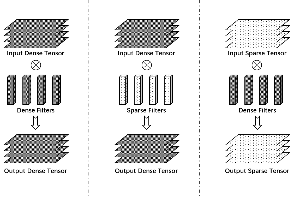
Figure 1: (a): standard convolution operator; (b): Sparse Filter CNN; (c) Sparse Input CNN.

On the other hand, modern CPUs typically possess multiple processors access to shared memory. To further accelerate the inference procedure, we make use of OpenMP [9] to realize multi-core parallelism. The following bulleted points are used to summarize our key contributions.

• We present a new accelerated Sparse CNN inference framework concentrating on CPUs. Our framework performs efficiently, supports varying sparse modules, i.e., either input or filter weights as sparse format, and is friendly to multi-processors parallelism.

• Instead of CSR(C) format, we make use of a slightly different sparse format, i.e., Liblinear sparse format [10]. We extend the Liblinear sparse format to represent three-dimensional (3-D) and four-dimensional 4-D tensor decently, design and develop a set of specialized sparse operators to achieve exact and efficient convolutional operation.

• The atomic operation of our framework is the inner product between sparse vector and dense vector, different from the matrix multiplication in existing sparse CNN inference frameworks, which typically require additional procedures to construct such operations. Besides, we present algorithms to optimize other related operations in this framework, e.g. fusing pooling operation into convolution operation.

2 Sparsity in CNN

In many scientific domains, the concept of tensor typically refers to single or multidimensional array, where both vector and matrix are its special instances. If most of elements in tensor are nonzero, then the tensor is considered dense, otherwise sparse. The sparsity in CNN is largely categorized into two classes: (i) sparse filter tensors, and (ii) sparse input tensor. The former one refers to that the trainable parameters of CNNs are sparse (including plentiful zero elements). Perhaps the most popular technique to generate sparse filters is to augment a penalty term to objective function during training, e.g. the $\ell_{1}$-regularized optimization [4] formulated as

$${\displaystyle\mathop{\operator@font{minimize}}_{x\in\mathbb{R}^{n}}}\ \{F(x)\ \stackrel{{\scriptstyle\mathclap{\mbox{\small def}}}}{{=}}\ f(x)+\lambda\left\|x\right\|_{1}\}$$ (1)

where $f(x)$ is the raw objective function of CNN, $\lambda>0$ is a weighting term. Problem (1) can be effectively solved deterministically [10, 1, 5] or stochastically [20, 32, 33, 34, 35] to produce pretty sparse solutions even with sparsity higher than 95% without sacrificing generalization accuracy on testing data. The latter one describes the characteristic in data of interest. In some domains, e.g., handwritten applications, data formed into 3-D tensor with numerous zero elements broadly exists [3, 19]. Therefore, utilizing such properties of sparsity to accelerate inference of CNN has practical realistic values.

3 Sparse Data Structure

The standard dense data structure allocates a contiguous memory space to save all entries in tensors. However, operations using such structures may be slow and inefficient when applied to large sparse tensors as processing, and memory are wasted on the zeroes. To address this issue, sparse data structure is introduced to store only non-zero elements that takes advantage of sparsity to avoid unnecessary operations.

CSR(C) format [30] is perhaps the most popular sparse format, which represents the sparse matrix by three arrays, as shown in Figure 2, (i) $B_{v}$: all the nonzero entries in this matrix; (ii) $B_{i}$: column indices of all stored nonzero entries; (iii) $B_{c}$: accumulated sum of non-zero element quantity (nnz) by each row starting with a 0. But these separate arrays in CSR(C) format may affect memory contiguity, and be not very elegant in real implementation.

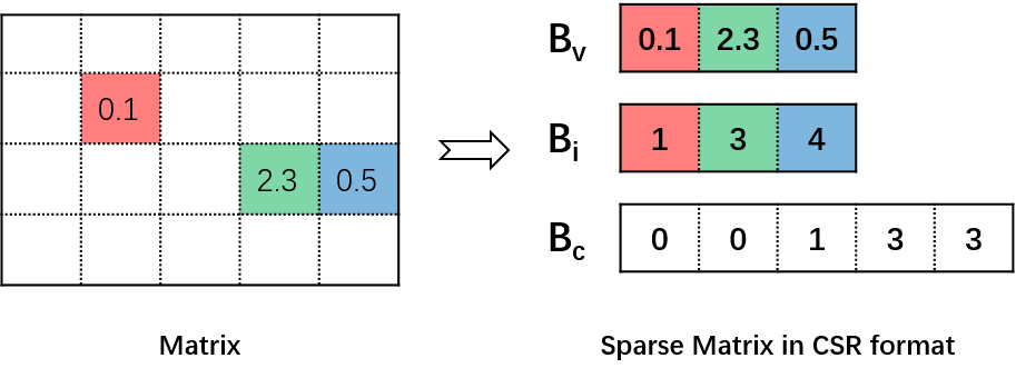
Figure 2: An example of sparse matrix in CSR(C) format.

On the other hand, Liblinear [10] implements a slightly different sparse format by utilizing a node struct, (referred as node throughout this paper), to pack values and indices of non-zero elements together, associated with an pointer array to store addresses of starting nodes for each column/row in sparse matrix. Such design is more elegant, and sometimes outperforms standard CSR(C) format, but is far from sufficiently supporting inference of CNN, which requires extension to 3-D tensor and 4-D tensor. To achieve sparse inference of CNN, we describe basic sparse vector and matrix data structure from Liblinear, and present our extended sparse 3-D and 4-D tensor data structures in the following.

• Node: Node is the fundamental data structure in FSCNN, consisting of two attributes, i.e. index and value, to mainly represent non-zero entries in sparse tensors, and some auxiliary components.

• Sparse Vector: A sparse vector can be naturally represented by an array of nodes for its non-zero entries with an auxiliary ending node with index as -1, shown as Figure 3.

  

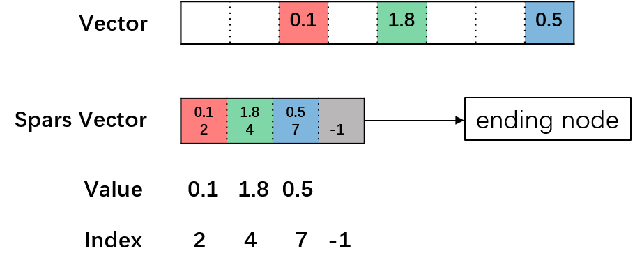
  Figure 3: An example of sparse vector.

• Sparse Matrix: A sparse matrix can be stored as a list of sparse vectors based on some prescribed order. For matrices, there exist two permissible orders, i.e., $O_{wh}$ and $O_{hw}$, corresponding to saving nodes along first each row (column) then each column (row). Besides, to facilitate access to a specific row (column), additional pointer array is established to store the addresses of the starting nodes of each row(column), illustrated in Figure 4.

  

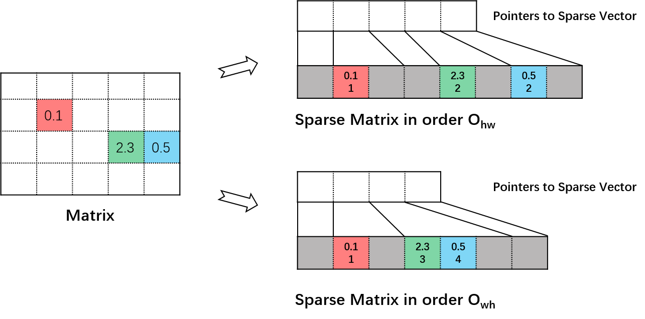
  Figure 4: An example of sparse matrix. Blank and gray squares in matrix represent zero elements and ending nodes respectively.

• Sparse 3-D Tensor: A sparse 3-D tensor can be viewed as a list of sparse matrices based on some predefined order, which represents the filters or input/output tensors in FSCNN. For 3-D tensors, totally six $(3!=6)$ feasible orders exist, namely, $O_{whc},O_{wch},O_{hwc},O_{hcw},O_{chw},O_{cwh}$, in which nodes are saved along specific axis order. For example, in $O_{chw}$, we save nodes along each channel first, height then and width finally. Similarly, to efficient access specific sparse matrix, we make use of an extra pointer array to save the starting node addresses of each matrix, shown in Figure 5.

  

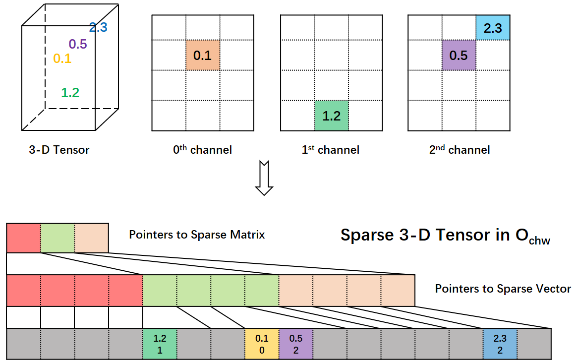
  Figure 5: An example of sparse 3-D tensor.

• Sparse 4-D Tensor: In FSCNN, sparse 4-D tensors are usually interpreted as a batch of input 3-D tensors, or a set of filters in convolutional layers. We make use of the similar logic to store sparse 4-D tensor as a list of sparse 3-D tensor under some order associated with a pointer array for starting nodes.

4 Sparse Tensor Operator

In this section, we present fundamental sparse tensor operators to form the entire inference of FSCNN based on the building blocks described in Section 3. The manner of convolutional operator is first presented. Then we show how to transpose sparse matrix, followed by an extension of operating sparse 3-D tensor transpose.

• Sparse Tensor Convolution: Convolution is the most fundamental operation in CNN, which operates on an input 3-D tensor and a 3-D filter tensor to yield a matrix. In FSCNN, we pay special interest to the case that either input tensor or filter tensor is sparse corresponding to Sparse Input CNN and Sparse Filter CNN respectively. To develop efficient sparse convolution, the manner in which we store 3-D tensors matters a lot. After several implementations, we reach a conclusion that perhaps the order $O_{chw}$ is the best, consistent with PyTorch [25]. We now state the sparse convolution as Algorithm 1 for the case that input tensor is dense, and filter tensor is sparse.

  Algorithm 1 Sparse Convolution between Dense Input 3-D Tensor $T_{I}$ and Sparse Filter Tensor $T_{F}$.

  1:Input: $T_{I}\in\mathbb{R}^{C_{I}\times H_{I}\times W_{I}}$, $T_{F}\in\mathbb{R}^{C_{F}\times H_{F}\times W_{F}}$, stride $S\in\mathbb{Z}^{+}$.

  2:Output: A matrix $M$ in dense format.

  3:Compute number of rows and columns of $M$ as $n_{h}$ and $n_{w}$:

  $$n_{h} \leftarrow(H_{I}-H_{F})/S+1;$$ (2)

  $$n_{w} \leftarrow(W_{I}-W_{F})/S+1.$$ (3)

  4:Declare a dense matrix $M$ of size $(n_{h},n_{w})$.

  5:for $i=0,1,\cdots,n_{h}-1$ do

  6:    for $j=0,1,\cdots,n_{w}-1$ do

  7:       Set $x\leftarrow 0$;

  8:       for $l=0,1,\cdots,W_{F}-1$ do

  9:          for $k=0,1,\cdots,H_{F}-1$ do

  10:             Update $x\leftarrow x+\text{dot}(T_{I}\verb|[l+jS][k+iS]|,T_{F}\verb|[l][k]|)$                  by Algorithm 2.                  

  11:       Append new value into $M$, i.e. $\verb|M[i][j]|\leftarrow x$.     

  12:return Dense Matrix $M$.

  As shown in Algorithm 1, we first compute the size of resulted matrix $M$ as line 3-4. Then each element of matrix is computed by summing $W_{F}H_{F}$ inner products between sparse vector from sparse filter $T_{F}$ and dense vector from input tensor $T_{I}$ , see line 7 to 11 in Algorithm 1. The crucial is the sparse inner product operator in line 10 by Algorithm 2. A concrete example of inner product between dense and sparse vector is shown in Figure 6, where float multiplications on zero elements are skipped to reduce the FLOPs. Resulting matrix $M$ is stored by $O_{wh}$ by the order of $T_{F}$ as $O_{chw}$ and Algorithm 1.

  Algorithm 2 Inner Product Between Dense Vector $v_{1}$ and Sparse Vector $v_{2}$.

  1:Input: Dense vector $v_{1}$, sparse vector $v_{2}$.

  2:Output: Real number $x$.

  3:Set $x\leftarrow 0$.

  4:while $v_{2}.\text{index}\neq-1$ do

  5:     Update $x\leftarrow x+v_{1}[v_{2}.\text{index}]\cdot v_{2}.\text{value}$.

  6:     Move pointer to next adjacent entry of $v_{2}$.

  7:return $x$.

  

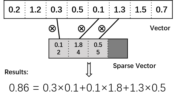
  Figure 6: An example of inner product between dense and sparse vector.

  For the case that input tensor $T_{I}$ is sparse and filter $T_{F}$ is dense, the logic of Algorithm 1 can be easily extended except setting the format of resulting matrix $M$. In this case, $M$ is stored in sparse format, which requires to check the value of $x$ on line 11, then append only nodes for non-zero $x$’s and auxiliary ending nodes for each row.

• Sparse Matrix Transpose: Sparse matrix transpose refers to switch a sparse matrix from order $O_{wh}$ to $O_{hw}$, or reversely. For simplicity, transpose from $O_{wh}$ to $O_{hw}$ is described in Algorithm 3, with a concrete example illustrated in Figure 7. At first, The indices of the starting point for each column in the new order $O_{hw}$ is calculated as $v$, which is also further used as progress tracker in the remaining transpose operation. Next, the nodes are rearranged from order of $O_{wh}$ into the order of $O_{hw}$ following the progress status shown in $v$. Meanwhile, $v$ is updated if any node is rearranged. The transpose operation completes by setting ending nodes for each column.

  Algorithm 3 Sparse Matrix Transpose from $O_{wh}$ to $O_{hw}$

  1:Input: Sparse matrix $M\in\mathbb{R}^{n_{w}\times n_{h}}$ in order $O_{wh}$.

  2:Output: Sparse matrix $M^{\prime}$ in order $O_{hw}$.

  3:Set $v\in\mathbb{Z}^{n_{w}+1}$ such that $v[i]$ is the number of nodes (including ending node) in $M$ by the $i$th column.

  4:Declare $M^{\prime}$ with appropriate space.

  5:for $i=0,1,\cdots,n_{h}-1$ do

  6:    for non-ending node in $i$-th row of $M$ do

  7:       Set

  $$\begin{split}M^{\prime}[v[\text{node.index}]]\text{.index}&\leftarrow i\\ M^{\prime}[v[\text{node.index}]]\text{.value}&\leftarrow\text{node.value}.\end{split}$$ (4)

  8:       Update $v[\text{node.index}]\leftarrow v[\text{node.index}]+1$     

  9:for $i=0,1,\cdots,n_{w}-1$ do

  10:    Set ending node:

  $$M^{\prime}[v[i]]\text{.index}\leftarrow-1$$ (5)

  11:return $M^{\prime}$.

  

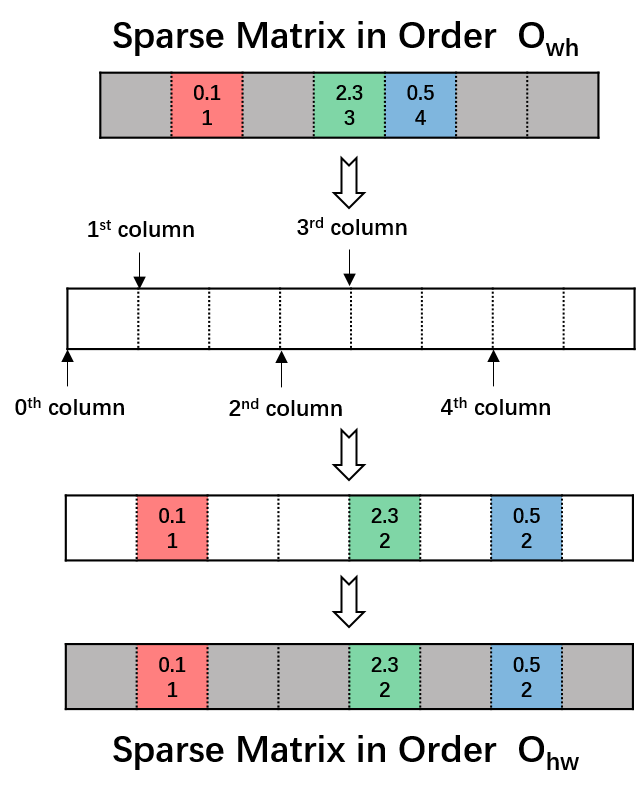
  Figure 7: An example of sparse matrix transpose from $O_{wh}$ to $O_{hw}$. The matrix is from Figure 4.

• Sparse 3-D Tensor Transpose: Similarly to sparse matrix transpose, sparse 3-D tensor transpose refers to convert one sparse 3-D tensor from one order to another. Algorithm 4 provides for a sparse 3-D tensor transpose operation, which transposes a 3-D tensor from order $O_{whc}$ to order $O_{chw}$. By the definition of sparse tensor and sparse matrix data structure, a tensor in order $O_{whc}$ can be regarded as number of channels’ sparse matrices in order $O_{wh}$ stacked together. Therefore, the sparse matrix transpose algorithm shown by Algorithm 3 is used to transpose each sparse matrix from order $O_{wh}$ to order $O_{hw}$ to form a tensor in $O_{hwc}$. Then, each node is iterated in $O_{hwc}$, reordering them if necessary to obtain a desired sparse tensor in order $O_{chw}$.

  Algorithm 4 Sparse Tensor Transpose from $O_{whc}$ to $O_{chw}$

  1:Input: Sparse 3-D tensor $T\in\mathbb{R}^{W\times H\times C}$ in order $O_{whc}$.

  2:Output: Sparse 3-D tensor $T^{\prime}$ in order $O_{chw}$.

  3:Declare $T^{\prime}$ with appropriate space.

  4:for each sparse matrix $M$ of order $O_{wh}$ in $T$  do

  5:    Transpose $M$ from $O_{wh}$ to $O_{hw}$ by Algorithm 3.

  6:for $w=0,1,\cdots,W-1$ do

  7:    for $h=0,1,\cdots,H-1$ do

  8:       for $c=0,1,\cdots,C-1$ do

  9:          if  $w$th column of $c$th $M$ reach non-ending node at $h$th height then

  10:             Copy this node into $T^{\prime}$ with index as $c$.                      

  11:return $T^{\prime}$.

5 Forward Pass of FSCNN

In this section, we assemble the basic data structures and operators described in previous sections to establish the entire forward pass of CNN. A standard CNN typically consists of stacking varied layers, including convolutional layers with(out) zero-padding, pooling layers, batch normalization layers [17], activation layers, among which convolutional layer is the crucial. Other layers can either operate independently or integrate sequentially into the convolutional layer. Our FSCNN considers the later one to avoid unnecessary memory access. Next, we describe the implementations of the above briefly based on the building blocks in Section 3 and 4.

• Convolutional layer: Each convolution layer contains an input tensor $T_{I}\in\mathbb{R}^{C_{I}\times H_{I}\times W_{I}}$, an output tensor $T_{O}\in\mathbb{R}^{C_{O}\times H_{O}\times W_{O}}$, and a set of filters $T_{F_{i}}\in\mathbb{R}^{C_{F_{i}}\times H_{F_{i}}\times W_{F_{i}i}}$ ($i\in[1,N]$ , where $N$ is the number of filters). These 3-D tensors satisfy the following properties, (i) $C_{I}=C_{F_{i}}$, for all $i\in[1,N]$, (ii) $C_{O}=N$. In Sparse Filter CNN variant, filter tensors $T_{F_{i}}$ are saved in sparse format, while in Sparse Input CNN variant, input tensor $T_{I}$ is saved in sparse format. To implement the forward pass of convolutional layer, FSCNN designs two approaches with different advantages, which are illustrated by Sparse Filter CNN variant as follows.

  The first approach is stated as Algorithm 5. At first, input tensor $T_{I}$ convolves with each filter to produce $N$ dense matrices of order $O_{wh}$ as line 4. Then these $N$ dense matrices are stacked along channel axis to form a dense tensor in the order of $O_{whc}$ as line 5. Next we transpose this dense tensor from order of $O_{whc}$ to $O_{chw}$ by Algorithm 4, and return it as the output volume $T_{O}$ finally.

  Algorithm 5 Forward Pass of Convolutional Layer I

  1:Input: $T_{I}\in\mathbb{R}^{C_{I}\times H_{I}\times W_{I}}$, $T_{F_{1}},T_{F_{2}},\cdots,T_{F_{N}}\in\mathbb{R}^{C_{F}\times H_{F}\times W_{F}}$, stride $S\in\mathbb{Z}^{+}$.

  2:Output: Dense 3-D tensor $T_{O}$ in order $O_{chw}$.

  3:for $i=1,2,\cdots,N$ do

  4:    Do convolution operation between dense $T_{I}$ and sparse $T_{F_{i}}$ by Algorithm 1.

  $$\text{Dense }M_{i}\leftarrow\text{tensor\_convolution}(T_{I},T_{F_{i}},S),$$

        where $M_{i}\in\mathbb{R}^{W_{O}\times H_{O}}$ is a dense matrix.

  5:Stack $M_{i}$’s together to form a dense tensor $T_{O^{\prime}}\in\mathbb{R}^{W_{O}\times H_{O}\times N}$.

  6:Transpose $T_{O^{\prime}}$ from order $O_{whc}$ into order $O_{chw}$ by Algorithm 4.

  $$T_{O}\leftarrow\text{transpose\_tensor}(T_{O^{\prime}})$$

  7:return $T_{O}$.

  The second approach stated as Algorithm 6 computes an output tensor more straightforward. Instead of convolving the input tensor with each filter iteratively to obtain multiple matrices, this approach directly compute the elements in output tensor.

  The first approach is friendly to multiprocessing on filter level over line 3 in Algorithm 5. Then the loop can be easily split into $N$ independent blocks, and executed by different processors simultaneously. However, the first method creates a temporary list save the output matrices, and processes additional steps of stacking matrices then doing tensor transpose to form output tensor . Hence it is both time and space consuming somewhat. On the other hand, although the second approach skips these extra procedures, its operations are entangled so that its loops can not be easily separated into multiple independent blocks for multiprocessing. This weakness may be overcome when performs inference on a batch of input tensors, where independent blocks over input tensors can be established.

  Algorithm 6 Forward Pass of Convolutional Layer II

  1:Input: $T_{I}\in\mathbb{R}^{C_{I}\times H_{I}\times W_{I}}$, $T_{F_{1}},T_{F_{2}},\cdots,T_{F_{N}}\in\mathbb{R}^{C_{F}\times H_{F}\times W_{F}}$, stride $S\in\mathbb{Z}^{+}$.

  2:Output: Dense 3-D tensor $T_{O}$ in order $O_{chw}$.

  3:Calculate $T_{O}$’s width $W_{O}$, height $H_{O}$ and channel $C_{O}$.

  $$W_{O} \leftarrow(W_{I}-W_{F_{1}})/S+1;$$ (6)

  $$H_{O} \leftarrow(H_{I}-H_{F_{1}})/S+1;$$ (7)

  $$C_{O} \leftarrow N.$$ (8)

  4:Declare a dense 3-D tensor $T_{O}$ of size $(W_{O},H_{O},C_{O})$.

  5:for $w=0,1,\cdots,W_{O}-1$ do

  6:    for $h=0,1,\cdots,H_{O}-1$ do

  7:       for $f=1,2,\cdots,C_{O}$ do

  8:          Set $x\leftarrow 0$;

  9:          for $l=0,1,\cdots,W_{F}-1$ do

  10:             for $k=0,1,\cdots,H_{F}-1$ do

  11:                Update: $x\leftarrow x+\text{dot}(T_{I}\verb|[l+wS][k+hS]|,T_{F_{f}}\verb|[l][k]|)$                        

  12:          Append new value into $T_{O}$, i.e., $T_{O}\verb|[w][h][f-1]|\leftarrow x$.            

  13:return Dense Tensor $T_{O}$.

  Our FSCNN contains a switch between these approaches to capitalize on the their advantages while avoiding the disadvantages. In particular, Algorithm 6 is called by default, unless the input batch size is relative small then Algorithm 5 is performed.

• Pooling Layers: Straightforward way to implement pooling layer is to perform pooling operation directly on the output tensor from previous layer. However, in Sparse Input CNN variant, it is difficult to locate the pooling region for sparse tensor of $O_{chw}$ because of its specific storage order. Therefore, for Sparse Input CNN, we merge pooling operations with convolutional operations stated as Algorithm 7, which is more efficient than doing convolutional and pooling operation separately. At first, the resulting matrix size is calculated using the parameters of convolutional and pooling operators. Then, convolutional operations are performed, as described above. However, during this operation, when an element is generated, it is used to update an array used for tracking values for each pooling region. When the pooling regions are complete, a sequence of values is constructed from the tracking value array. A matrix is generated in a sparse matrix data structure in order $O_{wh}$ by merging convolutional and pooling operations. An example of merged pooling operation is shown in Figure 8. As for Sparse Filter CNN variant, the above merging mechanism also works well, but we found out that doing convolutional and pooling operation separately performs more efficiently.

  Algorithm 7 Merge Pooling and Convolutional Operation

  1:Input: $T_{I}\in\mathbb{R}^{C_{I}\times H_{I}\times W_{I}}$, $T_{F}\in\mathbb{R}^{C_{F}\times H_{F}\times W_{F}}$, stride $S\in\mathbb{Z}^{+}$, pooling operator $P$ of size ($H_{P}$, $W_{P}$).

  2:Output: A matrix $M$ in dense format.

  3:Calculate the size of resulted matrix by only convolutional operation:

  $$n_{h,conv} \leftarrow(H_{I}-H_{F})/S+1;$$ (9)

  $$n_{w,conv} \leftarrow(W_{I}-W_{F})/S+1.$$ (10)

  4:Calculate $M$’s number of rows $n_{r}$ and columns $n_{c}$ after both convolutional and pooling operation.

  $$n_{h,pool} \leftarrow n_{h,conv}/H_{P};$$ (11)

  $$n_{w,pool} \leftarrow n_{w,conv}/W_{P}.$$ (12)

  5:Declare poolTrackValues as a size of $n_{w,pool}$ array to track desired values for each pooling region with size $H_{P}\times W_{P}$.

  6:for $i=0,1,\cdots,n_{h,conv}-1$ do

  7:    for $j=0,1,\cdots,n_{w,conv}-1$ do

  8:       Set $x\leftarrow 0$;

  9:       for $l=0,1,\cdots,W_{F}-1$ do

  10:          for $k=0,1,\cdots,H_{F}-1$ do

  11:             Update: $x\leftarrow x+\text{dot}(T_{I}\verb|[l+jS][k+iS]|,T_{F}\verb|[l][k]|)$                  

  12:       Update

  $$\verb|poolTrackValues[Pooling region of x]|$$

  by $x$ if needed.     

  13:    if $(i+1)\%H_{P}==0$ then

  14:       Insert values from poolTrackValues into $M$.

  15:       Reset poolTrackValues.     

  16:return $M$.

  

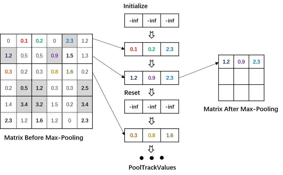
  Figure 8: An example of merged convolution and max-pooling operation as described in Algorithm 7. The bold number above gray grid represents the maximum entry in the pooling region.

• Other layers: FSCNN is flexible to padding operation, batch normalization and activation operations. Padding layers can be implemented by setting the output matrix with the same shape as the input tensor and shifting the indexing of input tensor in inner product left or right. Both batch normalizatiton and activation layer are additional functions applied to each elements in output tensor.

• Forward pass of FSCNN: The forward pass of sparse CNN becomes pertty straightforward once the above fundamental layers are well-defined. In general, layers are serially performed, and the output tensor of current layer serves as the input tensor of next layer.

6 Numerical Experiments

In this section, we numerically demonstrate the efficiency of FSCNN by comparing it with the state-of-the-art deep learning library PyTorch on popular CNN architectures VGG16 [30] and YOLO [27]. All experiments are conducted on a 64-bit machine with one Intel Xeon Platinum 8163 CPU with 16 processors and 32GB of main memory. PyTorch version is $0.4.1$ without GPU support. To be consistent with the default data type in PyTorch, our implementation uses 32-bit float numbers rather than 64-bit double numbers.

As described in Section 5, when the batch size of inputs is no greater than a threshold, FSCNN performs Algorithm 5, otherwise triggers Algorithm 6. This threshold is determined by the physical environment. In our experiments, we set it as $4$. We make use of OpenMP [9] to achieve multiprocessing programming. Generally, OpenMP exactly reduces the runtime of FSCNN in most cases, but when available CPU resource is limited, the cost of revoking OpenMP overcomes the benefits of multiprocessing. To achieve best performance, we turn off the OpenMP if CPU usage is larger than $0.95$ for Sparse Filter CNN.

6.1 Sparse Filter CNN Experiments

To illustrate the performance of Sparse Filter CNN comprehensively, we evaluate runtimes of Sparse Filter CNN for input as single or multiple instances under filter tensors of varying densities.

• Single Instance: We compare the performance between FSCNN and PyTorch on VGG16 and YOLO, shown in Table 1(a) and Table 1(b) respectively. It can be observed that FSCNN generally performs better than PyTorch when the density is no greater than $5\%$, indicating that Sparse Filter CNN effectively takes the advantage of high sparsity to accelerate inference. Especially when the density is less than $1\%$, Sparse Filter CNN outperforms PyTorch regardless of number of processes, and can achieve 1.5x to 3x speedups. Following the increase of density, FSCNN becomes slower since the benefits of sparse operations gradually disappear.

  density(%)	methods	number of processes running simultaneously
  		1	2	4	8	12	16
  1	FSCNN	0.1622	0.2437	0.3992	0.6909	0.9813	1.1903
  	PyTorch	0.5542	0.5580	0.6114	0.9007	1.3887	1.8918
  5	FSCNN	0.3067	0.3907	0.6394	1.1156	1.5435	1.7810
  	PyTorch	0.5531	0.5728	0.6001	0.8964	1.3864	1.8892
  10	FSCNN	0.6029	0.5934	0.9693	1.7233	2.4091	2.8139
  	PyTorch	0.5408	0.5638	0.5997	0.8870	1.3793	1.8875
  20	FSCNN	1.3414	0.9872	1.6748	3.0375	4.2691	5.1231
  	PyTorch	0.5418	0.5644	0.5963	0.8886	1.3749	1.8885
  50	FSCNN	4.6124	2.1707	3.7652	7.0721	9.8160	12.0788
  	PyTorch	0.5402	0.5645	0.5985	0.8841	1.3576	1.8860
  100	FSCNN	9.7058	4.1137	7.2583	13.8396	18.9156	23.4767
  	PyTorch	0.5463	0.5664	0.6005	0.8874	1.3369	1.8944

  (a) Runtime for VGG16.

  density(%)	methods	number of processes running simultaneously
  		1	2	4	8	12	16
  1	FSCNN	0.1803	0.2978	0.4577	0.7315	0.8765	0.9503
  	PyTorch	0.4884	0.5261	0.6230	1.2258	2.0018	2.7346
  5	FSCNN	0.3912	0.4583	0.6969	1.1374	1.4834	1.6194
  	PyTorch	0.4721	0.5280	0.6130	1.2173	1.9816	2.7419
  10	FSCNN	0.7359	0.6182	0.9794	1.6397	2.2129	2.4725
  	PyTorch	0.4925	0.5197	0.6047	1.2097	1.9690	2.7209
  20	FSCNN	1.4992	0.9536	1.5086	2.6650	3.6570	4.2331
  	PyTorch	0.4922	0.5140	0.6186	1.2135	1.9669	2.7250
  50	FSCNN	4.1250	1.8676	3.1060	5.8067	7.9827	9.6181
  	PyTorch	0.4941	0.5123	0.6056	1.2082	1.9175	2.7212
  100	FSCNN	8.8167	3.4057	5.7335	11.1056	15.1332	18.5831
  	PyTorch	0.4956	0.5258	0.6126	1.2250	1.8401	2.7353

  (b) Runtime for YOLO.

  Table 1: Runtimes of FSCNN and PyTorch under the architecture of (a) VGG16 (b) YOLO with different densities and number of processes running simultaneously.  FSCNN is set as Sparse Filter CNN variant.

• Multiple Instances: To explore the performance of Sparse Filter CNN given a batch of input tensors, we create Table 2(a) and 2(b) to present the runtimes on VGG16 and YOLO respectively. We can see that when the density is no larger than $5\%$, Sparse Filter CNN runs faster than other approach with one exception, i.e., the test of density as $5\%$ with batch size being 4. Even if density increases up to $20\%$, Sparse Filter CNN still achieves faster inference than PyTorch on YOLO when batch size equals to $16$ or $32$. This verifies the efficiency of underlying forward pass in Algorithm 6. Particularly, when density equals to $1\%$ and batch size is larger than $8$, Sparse Filter CNN can achieves roughly 6x speedups on both VGG16 and YOLO.

  density(%)	methods	batch size
  		1	2	4	8	16	32	64
  1	FSCNN	0.1394	0.3124	0.6214	0.7828	1.1650	2.2829	4.5582
  	PyTorch	0.5413	0.9982	1.8448	3.4790	6.7911	13.5070	26.7536
  5	FSCNN	0.3159	0.6134	1.0934	1.6125	2.5824	5.1019	10.2115
  	PyTorch	0.5442	0.9813	1.8453	3.4805	6.8337	13.5011	26.7553
  10	FSCNN	0.5979	1.1789	2.1062	2.6579	4.0500	8.0308	16.1110
  	PyTorch	0.5427	0.9962	1.8509	3.4892	6.7933	13.4856	26.7686
  20	FSCNN	1.3436	2.6965	3.6095	4.8044	6.7654	13.5081	27.0243
  	PyTorch	0.5428	0.9594	1.8275	3.5040	6.8366	13.5211	26.6894
  50	FSCNN	4.4832	9.3022	14.9400	11.3700	13.7979	27.5494	55.0434
  	PyTorch	0.5410	0.9876	1.8414	3.4889	6.8329	13.4898	26.7946
  100	FSCNN	9.7428	19.4605	38.2397	22.2444	24.7809	49.6027	99.3588
  	PyTorch	0.5517	1.0005	1.8418	3.4857	6.8532	13.5203	26.6328

  (a) Runtime for VGG16.

  density(%)	methods	batch size
  		1	2	4	8	16	32	64
  1	FSCNN	0.1785	0.3820	0.7946	0.7581	1.1605	2.3004	4.6041
  	PyTorch	0.4582	0.8680	1.6231	2.9958	5.7639	11.3392	23.0086
  5	FSCNN	0.3959	0.8375	1.7294	1.4390	2.1726	4.3269	8.7502
  	PyTorch	0.4869	0.8716	1.6311	3.0023	5.7948	11.4490	22.9784
  10	FSCNN	0.7364	1.5338	3.0927	2.3183	3.2735	6.5320	13.0444
  	PyTorch	0.4888	0.8696	1.6326	3.0095	5.7911	11.4212	23.0659
  20	FSCNN	1.4927	3.0760	6.2619	4.0802	5.2731	10.5313	21.0404
  	PyTorch	0.4907	0.8714	1.6355	3.0035	5.8353	11.4885	22.9948
  50	FSCNN	4.1997	8.1943	16.7630	9.7099	11.3508	22.6907	45.3361
  	PyTorch	0.4883	0.8663	1.6524	3.0169	5.8191	11.4623	22.9997
  100	FSCNN	8.8026	17.9287	34.9626	19.4020	21.2747	42.5343	85.1374
  	PyTorch	0.4900	0.8759	1.6315	3.0023	5.8114	11.4506	23.0047

  (b) Runtime for YOLO.

  Table 2: Runtimes of FSCNN and PyTorch under the architecture of (a) VGG16 (b) YOLO with different batch sizes.  FSCNN is set as Sparse Filter CNN variant.

6.2 Sparse Input CNN Experiments

In this section, we investigate the performance of Sparse Input CNN variant which assumes input tensor is sparse and filters are dense. To receive significant computational benefits from sparsity, the input tensor typically supposed to be highly sparse. Similar to the Sparse Filter CNN experiments, we select the density candidates as $0.01$, $0.05$, $0.1$, $0.2$, $0.5$ and $1$ of input tensor to evaluate the performance of Sparse Input CNN.

model	method	density (%)
		1	5	10	20	50	100
VGG16	FSCNN	1.1582	1.3453	1.3748	1.3873	1.3923	1.3721
	PyTorch	0.5412	0.5423	0.5454	0.5443	0.5449	0.5439
YOLO	FSCNN	1.5754	1.5833	1.5952	1.6061	1.6241	1.5885
	PyTorch	0.4820	0.4685	0.4707	0.4971	0.4691	0.4692

Table 3: Runtime of FSCNN and PyTorch on VGG16 and YOLO. FSCNN is set as Sparse Input CNN.

Table 3 shows the runtimes of Sparse Input CNN and PyTorch under different densities, where PyTorch performs faster than FSCNN on every test of VGG16 and YOLO. There are a few reasons as follows:

• VGG16 and YOLO consists of stacking a large number of convolutional layers. Even though the input tensor of the first convolutional layer is assumed as sparse, the sparsity of intermediate layers decays dramatically because of the convolution operation. Therefore, the gain from sparse operations vanishes gradually during forward pass. For a clear illustration, we create Figure 9 to present the evolution of densities of input tensors over each convolutional layer for VGG16 and YOLO, on which the input tensors generally becomes denser and denser.

  

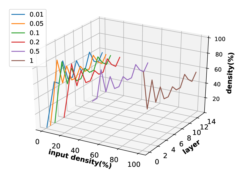
  (a) VGG16

  

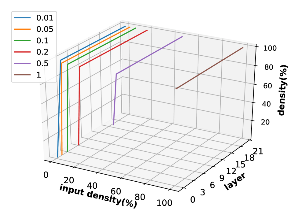
  (b) YOLO

  Figure 9: Density at each layer for (a) VGG16; (b) YOLO with different densities of input tensor.

• Activation and batch normalization layers also affects the sparsity a lot. As shown in Figure 9(a), the density curve of VGG16 fluctuates fiercely, because of the existence of ReLu activation function in VGG16. ReLu projects negative entries back to zero, so that the sparsity can be somehow promoted. On the contrast, YOLO makes use of LeakyReLU [24] and batch normalization, so that the density rapidly increases to $100\%$ only after a few convolutional layers, shown in Figure 9(b).

  To verify the above statements, we remove activation functions and batch normalization layers from VGG16 and YOLO, then record the runtime in Table 4 and the density evolution in Figure 10. VGG16 without ReLU runs slower than standard VGG16, which can be interpreted by the density curves that VGG16 with ReLU tends to possess sparser input tensors, so that Sparse Input CNN receives more computational benefits. Therefore, to let Sparse Input CNN achieve the best performance, it is recommended to construct a shallow convolutional neural network stacking by a small number of convolutional layers, and carefully select the activation functions.

  

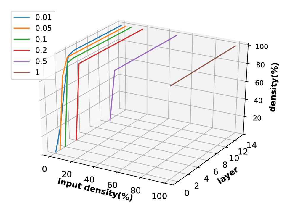
  (a) VGG16

  

  (b) YOLO

  Figure 10: Density at each layer for (a) VGG16; (b) YOLO with different densities of input . We remove the activation layers and batch normalizations from VGG16 and YOLO.

model	method	density
		1	5	10	20	50	100
VGG16 (-ReLU)	FSCNN	1.6478	1.9160	1.9419	1.9516	1.9638	1.9436
	PyTorch	0.5262	0.5308	0.4970	0.5441	0.5288	0.5291
YOLO (-BN, -LeakyReLU)	FSCNN	1.5957	1.6767	1.6869	1.6941	1.7138	1.6763
	PyTorch	0.4358	0.4347	0.4361	0.4356	0.4354	0.4353

Table 4: Density of output tensor and runtime for Sparse Input CNN on VGG16 and YOLO. We remove the activation layers and batch normalizations from VGG16 and YOLO.

References

- [1] Galen Andrew and Jianfeng Gao. Scalable training of l1-regularized log-linear models. In Proceedings of the 24th international conference on Machine learning, pages 33–40. ACM, 2007.
- [2] Sajid Anwar, Kyuyeon Hwang, and Wonyong Sung. Structured pruning of deep convolutional neural networks. ACM Journal on Emerging Technologies in Computing Systems (JETC), 13(3):32, 2017.
- [3] Kai Chen, Li Tian, Haisong Ding, Meng Cai, Lei Sun, Sen Liang, and Qiang Huo. A compact cnn-dblstm based character model for online handwritten chinese text recognition. 2017 14th IAPR International Conference on Document Analysis and Recognition (ICDAR), 01:1068–1073, 2017.
- [4] Tianyi Chen. A Fast Reduced-Space Algorithmic Framework for Sparse Optimization. PhD thesis, Johns Hopkins University, 2018.
- [5] Tianyi Chen, Frank E Curtis, and Daniel P Robinson. A reduced-space algorithm for minimizing ell_1-regularized convex functions. SIAM Journal on Optimization, 27(3):1583–1610, 2017.
- [6] Xuhao Chen. Escoin: Efficient sparse convolutional neural network inference on gpus, 2018.
- [7] Yu Cheng, Duo Wang, Pan Zhou, and Tao Zhang. A survey of model compression and acceleration for deep neural networks. arXiv preprint arXiv:1710.09282, 2017.
- [8] François Chollet. Xception: Deep learning with depthwise separable convolutions. In Proceedings of the IEEE conference on computer vision and pattern recognition, pages 1251–1258, 2017.
- [9] Leonardo Dagum and Ramesh Menon. Openmp: An industry-standard api for shared-memory programming. Computing in Science & Engineering, (1):46–55, 1998.
- [10] Rong-En Fan, Kai-Wei Chang, Cho-Jui Hsieh, Xiang-Rui Wang, and Chih-Jen Lin. Liblinear: A library for large linear classification. Journal of machine learning research, 9(Aug):1871–1874, 2008.
- [11] Ross Girshick, Jeff Donahue, Trevor Darrell, and Jitendra Malik. Rich feature hierarchies for accurate object detection and semantic segmentation. In Proceedings of the IEEE conference on computer vision and pattern recognition, pages 580–587, 2014.
- [12] Song Han, Xingyu Liu, Huizi Mao, Jing Pu, Ardavan Pedram, Mark A Horowitz, and William J Dally. Eie: efficient inference engine on compressed deep neural network. In 2016 ACM/IEEE 43rd Annual International Symposium on Computer Architecture (ISCA), pages 243–254. IEEE, 2016.
- [13] Song Han, Huizi Mao, and William J Dally. Deep compression: Compressing deep neural networks with pruning, trained quantization and huffman coding. arXiv preprint arXiv:1510.00149, 2015.
- [14] Song Han, Jeff Pool, John Tran, and William Dally. Learning both weights and connections for efficient neural network. In Advances in neural information processing systems, pages 1135–1143, 2015.
- [15] Yihui He, Xiangyu Zhang, and Jian Sun. Channel pruning for accelerating very deep neural networks. In Proceedings of the IEEE International Conference on Computer Vision, pages 1389–1397, 2017.
- [16] Andrew G Howard, Menglong Zhu, Bo Chen, Dmitry Kalenichenko, Weijun Wang, Tobias Weyand, Marco Andreetto, and Hartwig Adam. Mobilenets: Efficient convolutional neural networks for mobile vision applications. arXiv preprint arXiv:1704.04861, 2017.
- [17] Sergey Ioffe and Christian Szegedy. Batch normalization: Accelerating deep network training by reducing internal covariate shift. arXiv preprint arXiv:1502.03167, 2015.
- [18] Max Jaderberg, Andrea Vedaldi, and Andrew Zisserman. Speeding up convolutional neural networks with low rank expansions. arXiv preprint arXiv:1405.3866, 2014.
- [19] Bo Ji and Tianyi Chen. Generative adversarial network for handwritten text, 2019.
- [20] dong Jia, Liang Zhao, Lian Zhang, Juncai He, and Jinchao Xu. irda method for sparse convolutional neural networks. 2018.
- [21] Alex Krizhevsky, Ilya Sutskever, and Geoffrey E Hinton. Imagenet classification with deep convolutional neural networks. In Advances in neural information processing systems, pages 1097–1105, 2012.
- [22] Nicholas D Lane, Sourav Bhattacharya, Petko Georgiev, Claudio Forlivesi, Lei Jiao, Lorena Qendro, and Fahim Kawsar. Deepx: A software accelerator for low-power deep learning inference on mobile devices. In Proceedings of the 15th International Conference on Information Processing in Sensor Networks, page 23. IEEE Press, 2016.
- [23] Baoyuan Liu, Min Wang, Hassan Foroosh, Marshall Tappen, and Marianna Pensky. Sparse convolutional neural networks. In Proceedings of the IEEE Conference on Computer Vision and Pattern Recognition, pages 806–814, 2015.
- [24] Andrew L Maas, Awni Y Hannun, and Andrew Y Ng. Rectifier nonlinearities improve neural network acoustic models. In Proc. icml, volume 30, page 3, 2013.
- [25] Adam Paszke, Sam Gross, Soumith Chintala, Gregory Chanan, Edward Yang, Zachary DeVito, Zeming Lin, Alban Desmaison, Luca Antiga, and Adam Lerer. Automatic differentiation in pytorch. 2017.
- [26] Mohammad Rastegari, Vicente Ordonez, Joseph Redmon, and Ali Farhadi. Xnor-net: Imagenet classification using binary convolutional neural networks. In European Conference on Computer Vision, pages 525–542. Springer, 2016.
- [27] Joseph Redmon, Santosh Divvala, Ross Girshick, and Ali Farhadi. You only look once: Unified, real-time object detection. In Proceedings of the IEEE conference on computer vision and pattern recognition, pages 779–788, 2016.
- [28] Joseph Redmon and Ali Farhadi. Yolo9000: better, faster, stronger. In Proceedings of the IEEE conference on computer vision and pattern recognition, pages 7263–7271, 2017.
- [29] Yousef Saad. Iterative methods for sparse linear systems, volume 82. siam, 2003.
- [30] Karen Simonyan and Andrew Zisserman. Very deep convolutional networks for large-scale image recognition. arXiv preprint arXiv:1409.1556, 2014.
- [31] Bichen Wu, Alvin Wan, Xiangyu Yue, Peter Jin, Sicheng Zhao, Noah Golmant, Amir Gholaminejad, Joseph Gonzalez, and Kurt Keutzer. Shift: A zero flop, zero parameter alternative to spatial convolutions. In Proceedings of the IEEE Conference on Computer Vision and Pattern Recognition, pages 9127–9135, 2018.
- [32] Lin Xiao. Dual averaging methods for regularized stochastic learning and online optimization. Journal of Machine Learning Research, 11(Oct):2543–2596, 2010.
- [33] Lin Xiao and Tong Zhang. A proximal stochastic gradient method with progressive variance reduction. SIAM Journal on Optimization, 24(4):2057–2075, 2014.
- [34] Tianyi Chen, Tianyu Ding, Bo Ji, Guanyi Wang, Yixin Shi, Jing Tian, Sheng Yi, Xiao Tu, and Zhihui Zhu. Orthant based proximal stochastic gradient method for l1-Regularized optimization. Joint European Conference on Machine Learning and Knowledge Discovery in Databases, 2021.
- [35] Tianyi Chen, Bo Ji, Yixin Shi, Tianyu Ding, Biyi Fang, Sheng Yi, and Xiao Tu. Neural network compression via sparse optimization. arXiv preprint arXiv:2011.04868, 2020.