Iterative RNDOP-Optimal Anchor Placement for Beyond Convex Hull ToA-based Localization: Performance Bounds and Heuristic Algorithms

Raghunandan M. Rao, , Don-Roberts Emenonye, 
R. M. Rao is currently at Amazon Lab 126, Sunnyvale, CA, USA, 94086. This work was undertaken before joining Amazon in his capacity as an independent scholar and does not relate to his current role at Amazon. All findings and opinions in the paper are the author’s own and do not reflect the opinions of his employer (e-mail: raghumr@vt.edu).D.- R. Emenonye is affiliated with the Wireless@VT research group, Bradley Department of ECE, Virginia Tech, Blacksburg, VA, USA 24061 (email: donroberts@vt.edu).
Abstract

Localizing targets outside the anchors’ convex hull is an understudied but prevalent scenario in vehicle-centric, UAV-based, and self-localization applications. Considering such scenarios, this paper studies the optimal anchor placement problem for Time-of-Arrival (ToA)-based localization schemes such that the worst-case Dilution of Precision (DOP) is minimized. Building on prior results on DOP scaling laws for beyond convex hull ToA-based localization, we propose a novel metric termed the Range-Normalized DOP (RNDOP). We show that the worst-case DOP-optimal anchor placement problem simplifies to a min-max RNDOP-optimal anchor placement problem. Unfortunately, this formulation results in a non-convex and intractable problem under realistic constraints. To overcome this, we propose iterative anchor addition schemes, which result in a tractable albeit non-convex problem. By exploiting the structure arising from the resultant rank-1 update, we devise three heuristic schemes with varying performance-complexity tradeoffs. In addition, we also derive the upper and lower bounds for scenarios where we are placing anchors to optimize the worst-case (a) 3D positioning error and (b) 2D positioning error. We build on these results to design a cohesive iterative algorithmic framework for robust anchor placement and then discuss the computational complexity of the proposed schemes. Using numerical results, we validate the accuracy of our theoretical results. We also present comprehensive Monte-Carlo simulation results to compare the positioning error and execution time performance of each iterative scheme, discuss the tradeoffs, and provide valuable system design insights for beyond convex hull localization scenarios.

Index Terms:
Dilution of Precision (DOP), Beyond Convex Hull Localization, Range-Normalized DOP (RNDOP), Anchor Placement, Time-of-Arrival (ToA).

I Introduction

Localization applications are pervasive in the 5G and beyond-5G era, especially in consumer electronics, industrial, and defense sectors. In part due to the success of geolocation GPS and GNSS, consumers of wireless technology have increasing expectations regarding the reliability and accuracy of the location estimates in unprecedented deployments. Vehicle-centric localization is one such scenario that has been actively pursued by auto manufacturers and the wireless industry [1], wherein the target locations are estimated relative to the vehicle. This is in contrast with localizing targets on a local/global map, which is the typical approach in currently deployed positioning systems.

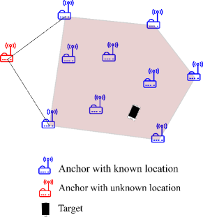
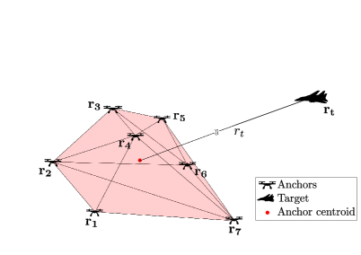
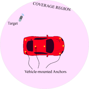
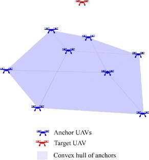
A vehicle-centric approach is crucial in applications such as autonomous driving [2], vehicle safety, keyless locking/unlocking [1], smart parking [3], etc. It is also useful for unmanned aerial vehicle (UAV)-based applications such as distributed UAV swarm coordination [4], autonomous takeoff and landing, and disaster assistance [5]. To enable autonomous vehicular operation, multiple anchors are deployed on the vehicle to track targets that are typically located outside the vehicle [6], as shown in Fig. 1(a). In other words, the targets are outside the convex hull formed by the anchor locations (henceforth referred to as a ‘beyond convex hull’ localization scenario) [7]. Such conditions also arise in (a) UAV-based localization applications for swarm coordination (Fig. 1(b)), and (b) self-localization where-in a new anchor needs to be localized relative to existing anchors in a wireless sensor network (Fig. 1(c)).

The target’s location can be estimated using measurements such as Time-of-Arrival (ToA) [7, 8], Time-Difference-of-Arrival (TDoA) [9], received signal strength (RSS) [10], and Angle-of-Arrival (AoA) typically fused with ToA or TDoA. Among these methods, ToA-based and TDoA-based localization provides robust range error performance in high multipath scenarios that accompany typical Non-Line of Sight (NLoS) wireless propagation environments. The state-of-the-art ranging methods using low-cost technologies such as ultrawideband (UWB) [11], which use high bandwidth, low power pulses that is capable of precise location estimates for moderate distances between the anchor and the target. If all the anchors are adequately time-synchronized, ToA-based algorithms have superior positioning performance when compared to TDoA-based schemes when the target is outside the anchors’ convex hull111Intuitively, this is because locus of the target in ToA is a circle that has a bounded region, whereas that in the case of TDoA is a hyperbola, an unbounded region [12]. In this paper, we seek to optimize anchor locations to minimize the worst-case positioning error in vehicle-centric ToA-based localization scenarios, where the target is located beyond the anchors’ convex hull.
Refer to caption
(a)
Refer to caption
(b)
Refer to caption
(c)
Figure 1: Illustration of beyond convex-hull localization scenarios. (a) Vehicle-centric localization, wherein multiple onboard vehicular sensors are used to localize exterior targets, (b) UAV-based localization, where a cluster of UAVs collaboratively localize targets outside the cluster, and (c) Anchor self-localization, where a new anchor joining a network has to position itself relative to the active anchors in the network.

I-A Related Work

Several prior works have studied anchor placement optimization techniques to minimize positioning error-related metrics. The localization error is a function of the measurement error, and the anchor locations relative to the target. The latter is often quantified by a dimensionless metric termed as the Dilution of Precision (DOP) [13]. Therefore, localization accuracy can be improved using (a) robust protocols and signal processing algorithms to reduce measurement error [14], and (b) by geometrically placing anchors such that the overall impact of measurement error on localization error is reduced.

The optimal anchor placement for TOA-based single static target localization is derived in [15] for the 2D case, and [16] for the 3D case. Sahu at al. [17] propose a unified mathematical framework based on alternating direction method of multipliers (ADMM) to design the optimal anchor geometry for ToA, AOA, RSS-based localization of a single target. Sheng et al. [8] analyze the optimal anchor placement problem for localizing two targets on the 2D plane using a common set of anchors. Fang et al. [18] study the optimal sensor placement problem for AOA-based localization where a single target and multiple anchors are constrained to lie within a circular region, while ensuring a minimum separation between all nodes. Using the notion of D-optimality, they formulate a constrained optimization problem where the constraints are related to the maximum feasible angle and the optimal separation angle. Panwar et al. [19] study the optimal sensor placement for hybrid TOA-RSS-AOA localization scenarios, and propose a solution based on the majorization-minimization (MM) technique.

However, for localizing multiple mobile targets, minimizing the positioning error for all targets at all possible locations in the coverage region is impossible. Therefore, state-of-the art works study, design, and characterize the performance of algorithms to minimize the weighted average of the localization error of targets in a region of interest, using theoretical and numerical approaches [20, 21, 22, 23], as well as empirical design-tools approaches [24, 25]. Stefania et al. [20] design optimal anchor placement for indoor ToA-based localization schemes to track a target moving along a corridor with the minimum average mean square error (MSE) along the linear trajectory. The authors in [21] consider RSS-based positioning of a single target using multiple UAVs, and propose an average MSE-optimal anchor placement scheme for positioning a terrestrial user located uniformly at random in a circular region. Kirchhof [22] presents a binary- (BIM) and mixed-integer programming (MIP)-based framework for anchor placement in indoor localization deployment scenarios, using the DOP as a key metric. Xu et al. [23] study the optimal sensor placement for TOA-based placement problem for multi-target localization with shared sensors, wherein they characterize the Cramer-Rao Lower Bound (CRLB) of such systems. They propose a hybrid approach which involves theoretical aspects such as A-optimality as well as sub-optimal approaches that rely on numerical optimization algorithms.

I-B Contributions

A key consideration in anchor placement, from the geometrical standpoint, is the enclosing of the region of interest by the convex hull of anchors. Prior works have rigorously shown that localization error reduces when the targets are located inside the convex hull of anchor locations (see [26], [27], [28]). Due to the favorable geometry, prior works predominantly focus on designing efficient anchor placement schemes for interior convex hull localization scenarios. This regime does not hold in vehicle-centric localization where system designers are constrained to deploy anchors on the vehicles’ body (Fig. 1(a)). Similar conditions can arise in UAV-based localization, and self-localization scenarios as shown in Figs. 1(b) and 1(c) respectively. Since these systems are often deployed as autonomous systems, they need to have the capability to localize multiple targets outside the convex hull, which severely limits the applicability of prior works. To fill this knowledge gap, we make the following contributions in this work.

Range-Normalized DOP (RNDOP)

When the target lies outside the anchors’ convex hull, we showed in our prior work [7] that the DOP (𝖣𝖣\mathsf{D}) scales linearly with the distance from the anchors’ centroid (rtsubscript𝑟𝑡r_{t}). Firstly, we extend these results by deriving closed-form expressions of the 2D-DOP (for XY localization in 3D space), as a function of the azimuth angle, and its upper and lower bounds. Furthermore, we propose a novel metric termed Range-Normalized DOP (𝖱𝖱\mathsf{R}). Using the linear DOP scaling results and the definition of RNDOP, we demonstrate that a weighted DOP optimization problem can be simplified to a weighted RNDOP optimization problem, where the weighting function is a function of the azimuth and elevation angles.

Min-Max DOP-optimal Iterative Anchor Placement Schemes for 2D and 3D Positioning

Using the asymptotic equivalence between the weighted DOP and weighted RNDOP optimization problems, we show that a robust DOP-optimal anchor configuration is almost invariant to the targets’ distance as long as it is far away outside the anchors’ convex hull. We then formulate a min-max RNDOP-optimal anchor placement problem under practical conditions such as (a) minimum anchor separation constraints, that are often imposed to ensure adequate device isolation, UAV safety, etc., and (b) box constraints, that approximately model the shape of terrestrial vehicles (such as trucks/buses), and the airspace above tall buildings. Unfortunately, the resultant problem is non-convex and intractable. To overcome this, we propose an iterative scheme, where a single anchor is added to the existing set of anchors at each iteration to minimize the maximum RNDOP. Observing the structure of the recurrence relation, we propose two additional heuristic schemes: one based on the (a) trace, and (b) eigenvector of a matrix-valued function solely composed of the anchor coordinates. In the process, we derive the upper and lower bounds on (a) the achievable RNDOP at each iteration for 2D and 3D localization, and (b) the universal RNDOP bounds for 3D localization. Finally, we combine these schemes into a cohesive iterative algorithmic framework to obtain robust 2D and 3D RNDOP-optimal anchor configurations.

Complexity Analysis and Numerical Results

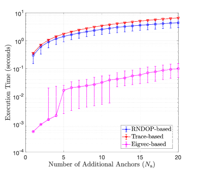
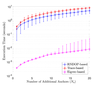
We analyze the worst-case computational complexity of each proposed variant, and show that for the Min-Max RNDOP and Trace-based heuristic schemes, the worst-case complexity is linear in the number of additional anchors to be added (Nasubscript𝑁aN_{\rm a}). We then use numerical results to validate the derived theoretical results, and develop a Monte-Carlo simulator to compare the positioning error and execution time performance of the proposed schemes across different computer configurations. We also provide useful insights by discussing the localization error-execution time tradeoff for all the proposed schemes, which can aid the design of practical beyond convex hull localization systems.

Notation

𝑿𝑿\bm{X} is a matrix, and 𝒙𝒙\bm{x} a column vector. 𝒙2subscriptnorm𝒙2\|\bm{x}\|_{2} and [𝒙]isubscriptdelimited-[]𝒙𝑖[\bm{x}]_{i} represent the 2-norm and ithsuperscript𝑖thi^{\text{th}} element of 𝒙𝒙\bm{x}. For a square matrix 𝑿𝑿\bm{X}, tr(𝑿)tr𝑿{\rm tr}(\bm{X}), 𝑿1superscript𝑿1\bm{X}^{-1} and 𝑿12superscript𝑿12\bm{X}^{\frac{1}{2}} represent the trace, inverse, and matrix square-root. The ordered eigenvalues of 𝑿𝑿\bm{X} are denoted by λ1(𝑿)λ2(𝑿)λn(𝑿)subscript𝜆1𝑿subscript𝜆2𝑿subscript𝜆𝑛𝑿\lambda_{1}(\bm{X})\leq\lambda_{2}(\bm{X})\leq\cdots\leq\lambda_{n}(\bm{X}), where λi(𝑿)subscript𝜆𝑖𝑿\lambda_{i}(\bm{X}) is the ithsuperscript𝑖𝑡i^{th} lowest eigenvalue, and its corresponding eigenvector is 𝒗i(𝑿)subscript𝒗𝑖𝑿\bm{v}_{i}(\bm{X}). λ+(𝑿)subscript𝜆𝑿\lambda_{+}(\bm{X}) and λ(𝑿)subscript𝜆𝑿\lambda_{-}(\bm{X}) represent the maximum and minimum eigenvalue, and 𝒗+(𝑿)subscript𝒗𝑿\bm{v}_{+}(\bm{X}) and 𝒗(𝑿)subscript𝒗𝑿\bm{v}_{-}(\bm{X}) represent their corresponding eigenvectors. Similarly, for symmetric matrices 𝑿𝑿\bm{X} and 𝒀𝒀\bm{Y}, λ+(𝑿,𝒀)subscript𝜆𝑿𝒀\lambda_{+}(\bm{X},\bm{Y}) and λ(𝑿,𝒀)subscript𝜆𝑿𝒀\lambda_{-}(\bm{X},\bm{Y}) denotes the maximum and minimum generalized eigenvalues of (𝑿,𝒀)𝑿𝒀(\bm{X},\bm{Y}). [𝑿]i,jsubscriptdelimited-[]𝑿𝑖𝑗[\bm{X}]_{i,j}, [𝑿]i,:subscriptdelimited-[]𝑿𝑖:[\bm{X}]_{i,:}, [𝑿]:,jsubscriptdelimited-[]𝑿:𝑗[\bm{X}]_{:,j} and [𝑿]i:m,j:nsubscriptdelimited-[]𝑿:𝑖𝑚𝑗:𝑛[\bm{X}]_{i:m,j:n} represent (i,j)thsuperscript𝑖𝑗th(i,j)^{\text{th}} element, ithsuperscript𝑖𝑡i^{th} row, jthsuperscript𝑗thj^{\text{th}} column, and the sub-matrix formed by choosing the row indices i:m:𝑖𝑚i:m and column indices j:n:𝑗𝑛j:n. 𝑰𝑰\bm{I} represents the identity matrix. 𝑰m×nsubscript𝑰𝑚𝑛\bm{I}_{m\times n} has the rows and columns of an m×m𝑚𝑚m\times m identity matrix, concatenated with nm𝑛𝑚n-m columns of all zeros. The set of real-valued n×n𝑛𝑛n\times n matrices and n×1𝑛1n\times 1 vectors are represented by n×nsuperscript𝑛𝑛\mathbb{R}^{n\times n} and n×1superscript𝑛1\mathbb{R}^{n\times 1} respectively, and that of n×n𝑛𝑛n\times n symmetric matrices are represented by 𝕊n×nsuperscript𝕊𝑛𝑛\mathbb{S}^{n\times n}. The set of positive definite and positive-semidefinite n×n𝑛𝑛n\times n matrices are represented by 𝕊+n×nsubscriptsuperscript𝕊𝑛𝑛\mathbb{S}^{n\times n}_{+} and 𝕊++n×nsubscriptsuperscript𝕊𝑛𝑛absent\mathbb{S}^{n\times n}_{++} respectively. X𝒰[𝒳]similar-to𝑋𝒰delimited-[]𝒳X\sim\mathcal{U}[\mathcal{X}] represents a random variable X𝑋X whose value is drawn uniformly at random from the set 𝒳𝒳\mathcal{X}.

II Mathematical Preliminaries

In this section, we mention a few useful results from matrix theory, for ease of exposition. These results are crucial for designing and characterizing the performance of algorithms presented in this paper.

Proposition 1.

(Sherman-Morrison formula [29]) Let 𝑿n×n𝑿superscript𝑛𝑛\bm{X}\in\mathbb{R}^{n\times n} be a non-singular matrix, and 𝒚,𝒛n𝒚𝒛superscript𝑛\bm{y},\bm{z}\in\mathbb{R}^{n} such that 𝒛T𝑿1𝒚1superscript𝒛𝑇superscript𝑿1𝒚1\bm{z}^{T}\bm{X}^{-1}\bm{y}\neq-1. Then, the inverse of the rank-1 update 𝒀=𝑿+𝒚𝒛T𝒀𝑿𝒚superscript𝒛𝑇\bm{Y}=\bm{X}+\bm{yz}^{T} is given by

𝒀1=𝑿1𝑿1𝒚𝒛T𝑿11+𝒛T𝑿1𝒚.superscript𝒀1superscript𝑿1superscript𝑿1𝒚superscript𝒛𝑇superscript𝑿11superscript𝒛𝑇superscript𝑿1𝒚\displaystyle\bm{Y}^{-1}=\bm{X}^{-1}-\tfrac{\bm{X}^{-1}\bm{yz}^{T}\bm{X}^{-1}}{1+\bm{z}^{T}\bm{X}^{-1}\bm{y}}. (1)
Proposition 2.

(Generalized eigenvalues/eigenvectors [30]) Suppose 𝑿𝕊n×n𝑿superscript𝕊𝑛𝑛\bm{X}\in\mathbb{S}^{n\times n}, and 𝒀𝕊+n×n𝒀subscriptsuperscript𝕊𝑛𝑛\bm{Y}\in\mathbb{S}^{n\times n}_{+}. Then, for a non-zero vector 𝒘n𝒘superscript𝑛\bm{w}\in\mathbb{R}^{n}, we have

λ(𝒁)subscript𝜆𝒁\displaystyle\lambda_{-}(\bm{Z}) =λ(𝑿,𝒀)𝒘T𝑿𝒘𝒘T𝒀𝒘λ+(𝑿,𝒀)=λ+(𝒁),absentsubscript𝜆𝑿𝒀superscript𝒘𝑇𝑿𝒘superscript𝒘𝑇𝒀𝒘subscript𝜆𝑿𝒀subscript𝜆𝒁\displaystyle=\lambda_{-}(\bm{X},\bm{Y})\leq\tfrac{\bm{w}^{T}\bm{Xw}}{\bm{w}^{T}\bm{Yw}}\leq\lambda_{+}(\bm{X},\bm{Y})=\lambda_{+}(\bm{Z}),

where 𝒁=𝒀12𝑿𝒀12𝒁superscript𝒀12𝑿superscript𝒀12\bm{Z}=\bm{Y}^{-\frac{1}{2}}\bm{XY}^{-\frac{1}{2}}. Furthermore, the upper bound is achieved when 𝒘=α𝒗+(𝒁)𝒘𝛼subscript𝒗𝒁\bm{w}=\alpha\bm{v}_{+}(\bm{Z}) and the lower bound when 𝒘=α𝒗(𝒁)𝒘𝛼subscript𝒗𝒁\bm{w}=\alpha\bm{v}_{-}(\bm{Z}), where α{0}𝛼0\alpha\in\mathbb{R}\setminus\{0\}.

Proposition 3.

(Eigenvalue bounds due to rank-1 perturbation [29], [31]) Let 𝒀=𝑿+ϵ𝒘𝒘T𝒀𝑿italic-ϵ𝒘superscript𝒘𝑇\bm{Y}=\bm{X}+\epsilon\bm{ww}^{T}, where 𝑿,𝒀n×n𝑿𝒀superscript𝑛𝑛\bm{X},\bm{Y}\in\mathbb{R}^{n\times n}, 𝒘n𝒘superscript𝑛\bm{w}\in\mathbb{R}^{n} such that 𝒘2=1subscriptnorm𝒘21\|\bm{w}\|_{2}=1, and ϵitalic-ϵ\epsilon\in\mathbb{R}. If ϵ<0italic-ϵ0\epsilon<0, we have

λ1(𝑿)ϵsubscript𝜆1𝑿italic-ϵabsent\displaystyle\lambda_{1}(\bm{X})-\epsilon\leq λ1(𝒀)λ1(𝑿)λ2(𝒀)λ2(𝑿)subscript𝜆1𝒀subscript𝜆1𝑿subscript𝜆2𝒀subscript𝜆2𝑿\displaystyle\lambda_{1}(\bm{Y})\leq\lambda_{1}(\bm{X})\leq\lambda_{2}(\bm{Y})\leq\lambda_{2}(\bm{X})\leq\cdots
λn(𝒀)λn(𝑿).absentsubscript𝜆𝑛𝒀subscript𝜆𝑛𝑿\displaystyle\leq\lambda_{n}(\bm{Y})\leq\lambda_{n}(\bm{X}). (2)

On the other hand, if ϵ>0italic-ϵ0\epsilon>0 then we have

λ1(𝑿)subscript𝜆1𝑿absent\displaystyle\lambda_{1}(\bm{X})\leq λ1(𝒀)λ2(𝑿)λ2(𝒀)λ3(𝑿)subscript𝜆1𝒀subscript𝜆2𝑿subscript𝜆2𝒀subscript𝜆3𝑿\displaystyle\lambda_{1}(\bm{Y})\leq\lambda_{2}(\bm{X})\leq\lambda_{2}(\bm{Y})\leq\lambda_{3}(\bm{X})\leq\cdots
λn(𝑿)λn(𝒀)λn(𝑿)+ϵ.absentsubscript𝜆𝑛𝑿subscript𝜆𝑛𝒀subscript𝜆𝑛𝑿italic-ϵ\displaystyle\leq\lambda_{n}(\bm{X})\leq\lambda_{n}(\bm{Y})\leq\lambda_{n}(\bm{X})+\epsilon. (3)

In both cases, there exists disubscript𝑑𝑖d_{i} for i=1,2,,n𝑖12𝑛i=1,2,\cdots,n such that

λi(𝒀)=λi(𝑿)+diϵ,i=1,2,,n,formulae-sequencesubscript𝜆𝑖𝒀subscript𝜆𝑖𝑿subscript𝑑𝑖italic-ϵ𝑖12𝑛\displaystyle\lambda_{i}(\bm{Y})=\lambda_{i}(\bm{X})+d_{i}\epsilon,i=1,2,\cdots,n, (4)

where 0di10subscript𝑑𝑖10\leq d_{i}\leq 1 and i=1ndi=1superscriptsubscript𝑖1𝑛subscript𝑑𝑖1\sum_{i=1}^{n}d_{i}=1.

Proposition 4.

Let 𝑿𝟑𝕊+3×3subscript𝑿3subscriptsuperscript𝕊33\bm{X_{3}}\in\mathbb{S}^{3\times 3}_{+}. The solution to the optimization problem

Λ=min𝑿𝟑superscriptΛsubscript𝑿3\displaystyle\Lambda^{*}=\underset{\bm{X_{3}}}{\min} tr(𝑿𝟑1)λ(𝑿𝟑1)trsubscriptsuperscript𝑿13subscript𝜆subscriptsuperscript𝑿13\displaystyle\ {\rm tr}(\bm{X}^{-1}_{\bm{3}})-\lambda_{-}(\bm{X}^{-1}_{\bm{3}}) (5)
s.t.formulae-sequencest\displaystyle{\rm s.t.\ } tr(𝑿𝟑)=Ktrsubscript𝑿3𝐾\displaystyle{\rm tr}(\bm{X_{3}})=K

is given by Λ=6tr(𝑿𝟑)=6KsuperscriptΛ6trsubscript𝑿36𝐾\Lambda^{*}=\frac{6}{{\rm tr}(\bm{X_{3}})}=\frac{6}{K}, which is achieved when its eigenvalues λi(𝑿𝟑)=K3subscript𝜆𝑖subscript𝑿3𝐾3\lambda_{i}(\bm{X_{3}})=\frac{K}{3} for i=1,2,3𝑖123i=1,2,3.

Comment 1.
Corollary 1.

Let 𝑿𝟐𝕊++2×2subscript𝑿2subscriptsuperscript𝕊22absent\bm{X_{2}}\in\mathbb{S}^{2\times 2}_{++}. The solution to the optimization problem

Λ=min𝑿𝟐superscriptΛsubscript𝑿2\displaystyle\Lambda^{*}=\underset{\bm{\bm{X_{2}}}}{\min} tr(𝑿𝟐1)λ(𝑿𝟐1)trsubscriptsuperscript𝑿12subscript𝜆subscriptsuperscript𝑿12\displaystyle\ {\rm tr}(\bm{X}^{-1}_{\bm{2}})-\lambda_{-}(\bm{X}^{-1}_{\bm{2}}) (6)
s.t.formulae-sequencest\displaystyle{\rm s.t.\ } tr(𝑿𝟐)=Ktrsubscript𝑿2𝐾\displaystyle{\rm tr}(\bm{X_{2}})=K

is given by Λ=4KsuperscriptΛ4𝐾\Lambda^{*}=\frac{4}{K}, which is achieved when its eigenvalues λi(𝑿𝟐)=K2subscript𝜆𝑖subscript𝑿2𝐾2\lambda_{i}(\bm{X_{2}})=\frac{K}{2} for i=1,2𝑖12i=1,2.

Proof.

The proof is similar to Proposition 4, and is omitted due to space constraints. ∎

III System Model

III-A Ranging Error Model

We consider a network of N𝑁N anchors which are used to determine the unknown position of a target in 3D space. All the anchor locations are assumed to be known, and the ithsuperscript𝑖𝑡i^{th} anchor is located at 𝒓𝒊=[xiyizi]T,i=1,2,,Nformulae-sequencesubscript𝒓𝒊superscriptdelimited-[]subscript𝑥𝑖subscript𝑦𝑖subscript𝑧𝑖𝑇𝑖12𝑁\bm{r_{i}}=[x_{i}\ y_{i}\ z_{i}]^{T},i=1,2,\cdots,N. The target’s unknown location is at 𝒓𝒕=[xtytzt]Tsubscript𝒓𝒕superscriptdelimited-[]subscript𝑥𝑡subscript𝑦𝑡subscript𝑧𝑡𝑇\bm{r_{t}}=[x_{t}\ y_{t}\ z_{t}]^{T}. The ithsuperscript𝑖𝑡i^{th} anchor measures the time-of-arrival (ToA) τisubscript𝜏𝑖\tau_{i} from the target (also referred to as ‘tag’) using two-way ranging mechanisms [14], which is given by [32]

τi=1c(𝒓𝒊𝒓𝒕2+wi), for i=1,2,,N,formulae-sequencesubscript𝜏𝑖1𝑐subscriptnormsubscript𝒓𝒊subscript𝒓𝒕2subscript𝑤𝑖 for 𝑖12𝑁\displaystyle\tau_{i}=\frac{1}{c}(\|\bm{r_{i}}-\bm{r_{t}}\|_{2}+w_{i}),\text{ for }i=1,2,\cdots,N, (7)

where c𝑐c is the velocity of light, wi𝒩(bi,σw2)similar-tosubscript𝑤𝑖𝒩subscript𝑏𝑖subscriptsuperscript𝜎2𝑤w_{i}\sim\mathcal{N}(b_{i},\sigma^{2}_{w}) is the ranging error, and bi>0subscript𝑏𝑖0b_{i}>0 is the range bias due to multipath.

III-B Localization Error and the Dilution of Precision (DOP)

For range-based localization schemes, the overall positioning error depends on the statistics of the ranging errors (wi,i=1,2,,Nformulae-sequencesubscript𝑤𝑖𝑖12𝑁w_{i},i=1,2,\cdots,N), as well as the anchor coordinates relative to the target. The Cramér-Rao Lower Bound (CRLB) for the localization error222This quantity is often also referred to as the Positioning Error Bound (PEB) in the literature. under (7) is given by [13]

Var([𝒓𝒕𝒓^𝒕]i)Varsubscriptdelimited-[]subscript𝒓𝒕subscriptbold-^𝒓𝒕𝑖\displaystyle{\rm Var}([\bm{r_{t}}-\bm{\hat{r}_{t}}]_{i}) [(𝑯T𝑾1𝑯)1]i,i,whereabsentsubscriptdelimited-[]superscriptsuperscript𝑯𝑇superscript𝑾1𝑯1𝑖𝑖where\displaystyle\geq\big{[}\big{(}\bm{H}^{T}\bm{W}^{-1}\bm{H}\big{)}^{-1}\big{]}_{i,i},\text{where } (8)
𝑯Tsuperscript𝑯𝑇\displaystyle\bm{H}^{T} =[𝒓𝒕𝒓𝟏𝒓𝒕𝒓𝟏2𝒓𝒕𝒓𝟐𝒓𝒕𝒓𝟐2𝒓𝒕𝒓𝑵𝒓𝒕𝒓𝑵2],andabsentsubscript𝒓𝒕subscript𝒓1subscriptnormsubscript𝒓𝒕subscript𝒓12subscript𝒓𝒕subscript𝒓2subscriptnormsubscript𝒓𝒕subscript𝒓22subscript𝒓𝒕subscript𝒓𝑵subscriptnormsubscript𝒓𝒕subscript𝒓𝑵2and\displaystyle=\big{[}\tfrac{\bm{r_{t}}-\bm{r_{1}}}{\|\bm{r_{t}}-\bm{r_{1}}\|_{2}}\ \ \tfrac{\bm{r_{t}}-\bm{r_{2}}}{\|\bm{r_{t}}-\bm{r_{2}}\|_{2}}\cdots\tfrac{\bm{r_{t}}-\bm{r_{N}}}{\|\bm{r_{t}}-\bm{r_{N}}\|_{2}}\big{]},\text{and } (9)
𝑾𝑾\displaystyle\bm{W} =𝔼[𝒘𝒘T],𝒘=[w1w2wN]T.formulae-sequenceabsent𝔼delimited-[]𝒘superscript𝒘𝑇𝒘superscriptdelimited-[]subscript𝑤1subscript𝑤2subscript𝑤𝑁𝑇\displaystyle=\mathbb{E}[\bm{ww}^{T}],\bm{w}=[w_{1}\ w_{2}\ \cdots w_{N}]^{T}. (10)

In this paper, we focus on ToA-based localization of far-away targets outside the convex hull of the anchor locations (henceforth referred to as ‘beyond convex hull’ localization scenarios) [7]. For far-away targets, we assume that

  • the bias of the range error on each anchor is the same, i.e. bi=bi=1,2,,Nformulae-sequencesubscript𝑏𝑖𝑏for-all𝑖12𝑁b_{i}=b\ \forall i=1,2,\cdots,N, and

  • the unbiased range error (wibi)subscript𝑤𝑖subscript𝑏𝑖(w_{i}-b_{i}) on each anchor are uncorrelated random variables.

Equal range bias for a far-away target is plausible since the multipath scattering geometry is likely to be highly correlated for all the anchors. Under these assumptions, we get 𝑾=(b2+σw2)𝑰𝑵𝑾superscript𝑏2subscriptsuperscript𝜎2𝑤subscript𝑰𝑵\bm{W}=(b^{2}+\sigma^{2}_{w})\bm{I}_{\bm{N}} and the CRLB expression in (8) simplifies to

Var([𝒓𝒕𝒓^𝒕]i)Varsubscriptdelimited-[]subscript𝒓𝒕subscriptbold-^𝒓𝒕𝑖\displaystyle{\rm Var}([\bm{r_{t}}-\bm{\hat{r}_{t}}]_{i}) (b2+σw2)[(𝑯T𝑯)1]i,i.absentsuperscript𝑏2subscriptsuperscript𝜎2𝑤subscriptdelimited-[]superscriptsuperscript𝑯𝑇𝑯1𝑖𝑖\displaystyle\geq(b^{2}+\sigma^{2}_{w})\big{[}\big{(}\bm{H}^{T}\bm{H}\big{)}^{-1}\big{]}_{i,i}. (11)

Thus, the positioning error bound (PEB) is given by

Var(𝒓𝒕𝒓^𝒕2)Varsubscriptnormsubscript𝒓𝒕subscriptbold-^𝒓𝒕2\displaystyle\sqrt{{\rm Var}(\|\bm{r_{t}}-\bm{\hat{r}_{t}}\|_{2})} (b2+σw2)×tr([𝑯T𝑯]1).absentsuperscript𝑏2subscriptsuperscript𝜎2𝑤trsuperscriptdelimited-[]superscript𝑯𝑇𝑯1\displaystyle\geq\sqrt{(b^{2}+\sigma^{2}_{w})\times\text{tr}([\bm{H}^{T}\bm{H}]^{-1})}. (12)

Thus, the PEB is dependent on (a) the statistics of range error (b,σw)𝑏subscript𝜎𝑤(b,\sigma_{w}), and the (b) geometrical placement of anchors relative to the target (𝑯)𝑯(\bm{H}). The impact of anchor placement on the target’s positioning error is quantified by the dimensionless metric termed as Dilution of Precision (DOP) [13]. It is defined in terms of 𝑸=[𝑯T𝑯]1𝑸superscriptdelimited-[]superscript𝑯𝑇𝑯1\bm{Q}=[\bm{H}^{T}\bm{H}]^{-1} below for 3D (𝖣𝗑𝗒𝗓subscript𝖣𝗑𝗒𝗓\mathsf{D_{xyz}}), and 2D (𝖣𝗑𝗒subscript𝖣𝗑𝗒\mathsf{D_{xy}}) localization.

𝖣𝗑𝗒𝗓subscript𝖣𝗑𝗒𝗓\displaystyle\mathsf{D_{xyz}} =tr(𝑸),absenttr𝑸\displaystyle=\sqrt{{\rm tr}(\bm{Q})}, (13)
𝖣𝗑𝗒subscript𝖣𝗑𝗒\displaystyle\mathsf{D_{xy}} =tr([𝑸]1:2,1:2).absenttrsubscriptdelimited-[]𝑸:121:2\displaystyle=\sqrt{{\rm tr}([\bm{Q}]_{1:2,1:2})}. (14)

DOP satisfies the following properties.

Property 1.

(Translational Invariance) The DOP does not change when all the anchors and the target are translated by a vector 𝚫𝒓𝚫𝒓\bm{\Delta r}.

Property 2.

(Scale Invariance) If the anchor and target coordinates are scaled by a factor of k𝑘k (k0𝑘0k\neq 0), then the DOP remains unchanged.

Using the definition of 𝑯𝑯\bm{H} in (9), Property 1 follows from the fact that the entries of 𝑯𝑯\bm{H} depend on the vector difference between the target and the anchor coordinates. On the other hand, Property 2 follows since the entries in 𝑯𝑯\bm{H} are normalized ratios of the anchor positions relative to the target.

III-C DOP and Range-Normalized DOP (RNDOP) in ToA-based Positioning of Far-Away Targets

Beyond convex hull localization is motivated by several practical use cases, such as using vehicular sensors to track outdoor targets [2, 7] (Fig. 1(a)), localization of UAVs using terrestrial vehicle-mounted anchors [33], and self-localization scenarios (Fig. 1(c)). Formally, the target is considered to be far-away if the following conditions are met, for i,j=1,2,,Nformulae-sequence𝑖𝑗12𝑁i,j=1,2,\cdots,N and ij𝑖𝑗i\neq j:

  1. 1.

    𝒓𝒊𝒓𝒕2𝒓𝒋𝒓𝒕2𝒓𝒕2subscriptnormsubscript𝒓𝒊subscript𝒓𝒕2subscriptnormsubscript𝒓𝒋subscript𝒓𝒕2subscriptnormsubscript𝒓𝒕2\|\bm{r_{i}}-\bm{r_{t}}\|_{2}\approx\|\bm{r_{j}}-\bm{r_{t}}\|_{2}\approx\|\bm{r_{t}}\|_{2}, and

  2. 2.

    𝒓𝒊𝒓𝒋2𝒓𝒊𝒓𝒕2much-less-thansubscriptnormsubscript𝒓𝒊subscript𝒓𝒋2subscriptnormsubscript𝒓𝒊subscript𝒓𝒕2\|\bm{r_{i}}-\bm{r_{j}}\|_{2}\ll\|\bm{r_{i}}-\bm{r_{t}}\|_{2}.

While the notion of ‘approximate equality’ in the above description is rather arbitrary, we will provide a formal working definition of the ‘far-away target’ scenario later in this section. Due to the translational invariance of the DOP, we have the following modeling assumption regarding the origin of the coordinate system.

Assumption 1.

The origin of the local coordinate system (LCS) is located at the centroid of the anchor locations, i.e. i=1N𝒓𝒊=𝟎superscriptsubscript𝑖1𝑁subscript𝒓𝒊0\sum_{i=1}^{N}\bm{r_{i}}=\bm{0}.

Refer to caption
Figure 2: 3D ToA-based localization of far-away targets. The anchors are mounted on UAVs, and the ithsuperscript𝑖thi^{\rm th} anchor is at 𝒓𝒊=(xi,yi,zi),i=1,2,,Nformulae-sequencesubscript𝒓𝒊subscript𝑥𝑖subscript𝑦𝑖subscript𝑧𝑖𝑖12𝑁\bm{r_{i}}=(x_{i},y_{i},z_{i}),i=1,2,\cdots,N such that all anchors are confined in a relatively small volume enclosed by their convex hull, such that i=1N𝒓𝒊=𝟎superscriptsubscript𝑖1𝑁subscript𝒓𝒊0\sum_{i=1}^{N}\bm{r_{i}}=\bm{0}. The target is far-away from the origin such that rt𝒓𝒕𝒓𝒊2subscript𝑟𝑡subscriptnormsubscript𝒓𝒕subscript𝒓𝒊2r_{t}\approx\|\bm{r_{t}}-\bm{r_{i}}\|_{2}.

For far-away targets outside the anchors’ convex hull, we have the following proposition.

Proposition 5.

In the far-away target regime, we have

𝑯T𝑯superscript𝑯𝑇𝑯\displaystyle\bm{H}^{T}\bm{H} 1rt2(𝑪+Nrt2𝒂𝒕(θ,ϕ)𝒂𝒕T(θ,ϕ))𝟎,absent1subscriptsuperscript𝑟2𝑡𝑪𝑁subscriptsuperscript𝑟2𝑡subscript𝒂𝒕𝜃italic-ϕsubscriptsuperscript𝒂𝑇𝒕𝜃italic-ϕsucceeds-or-equals0\displaystyle\approx\frac{1}{r^{2}_{t}}(\bm{C}+Nr^{2}_{t}\bm{a_{t}}(\theta,\phi)\bm{a}^{T}_{\bm{t}}(\theta,\phi))\succcurlyeq\bm{0}, (15)

where 𝑪=i=1N𝒓𝒊𝒓𝒊T𝑪superscriptsubscript𝑖1𝑁subscript𝒓𝒊subscriptsuperscript𝒓𝑇𝒊\bm{C}=\sum_{i=1}^{N}\bm{r_{i}r}^{T}_{\bm{i}}, 𝒓𝒕=rt𝒂𝒕(θ,ϕ)subscript𝒓𝒕subscript𝑟𝑡subscript𝒂𝒕𝜃italic-ϕ\bm{r_{t}}=r_{t}\bm{a_{t}}(\theta,\phi), and 𝒂𝒕(θ,ϕ)=[cosθsinϕsinθsinϕcosϕ]Tsubscript𝒂𝒕𝜃italic-ϕsuperscriptdelimited-[]𝜃italic-ϕ𝜃italic-ϕitalic-ϕ𝑇\bm{a_{t}}(\theta,\phi)=[\cos\theta\sin\phi\ \sin\theta\sin\phi\ \cos\phi]^{T}.

Proof.

Please refer [7, Proposition 1]. ∎

The above result can then be used to obtain a distinct ‘DOP scaling law’ for localization in all dimensions, as shown in the following theorem.

Theorem 1.

If rt1Nλ(𝑪1)much-greater-thansubscript𝑟𝑡1𝑁subscript𝜆superscript𝑪1r_{t}\gg\frac{1}{\sqrt{N\lambda_{-}(\bm{C}^{-1})}}, then 𝑸𝑸\bm{Q} scales linearly with rtsubscript𝑟𝑡r_{t} for a fixed target direction 𝒂𝒕=𝒓𝒕/𝒓𝒕2subscript𝒂𝒕subscript𝒓𝒕subscriptnormsubscript𝒓𝒕2\bm{a_{t}}=\bm{r_{t}}/\|\bm{r_{t}}\|_{2}, and is given by

𝑸=rt(𝑪1𝑪1𝒂𝒕𝒂𝒕T𝑪1𝒂𝒕T𝑪1𝒂𝒕).𝑸subscript𝑟𝑡superscript𝑪1superscript𝑪1subscript𝒂𝒕superscriptsubscript𝒂𝒕𝑇superscript𝑪1superscriptsubscript𝒂𝒕𝑇superscript𝑪1subscript𝒂𝒕\displaystyle\bm{Q}=r_{t}\Big{(}\bm{C}^{-1}-\tfrac{\bm{C}^{-1}\bm{a_{t}}\bm{a_{t}}^{T}\bm{C}^{-1}}{\bm{a_{t}}^{T}\bm{C}^{-1}\bm{a_{t}}}\Big{)}. (16)
Proof.

Please refer [7, Theorem 1].

Comment 2.

Using Proposition 5, we get 𝑸=(rt2𝑪+N𝒂𝒕𝒂𝒕T)1𝑸superscriptsubscriptsuperscript𝑟2𝑡𝑪𝑁subscript𝒂𝒕subscriptsuperscript𝒂𝑇𝒕1\bm{Q}=\big{(}r^{-2}_{t}\bm{C}+N\bm{a_{t}a}^{T}_{\bm{t}}\big{)}^{-1}. Using Proposition 1, we get

𝑸=rt2𝑪1rt2(𝑪1𝒂𝒕𝒂𝒕T𝑪1N1rt2+𝒂𝒕T𝑪1𝒂𝒕).𝑸subscriptsuperscript𝑟2𝑡superscript𝑪1subscriptsuperscript𝑟2𝑡superscript𝑪1subscript𝒂𝒕superscriptsubscript𝒂𝒕𝑇superscript𝑪1superscript𝑁1subscriptsuperscript𝑟2𝑡superscriptsubscript𝒂𝒕𝑇superscript𝑪1subscript𝒂𝒕\displaystyle\bm{Q}=r^{2}_{t}\bm{C}^{-1}-r^{2}_{t}\Big{(}\tfrac{\bm{C}^{-1}\bm{a_{t}a_{t}}^{T}\bm{C}^{-1}}{N^{-1}r^{-2}_{t}+\bm{a_{t}}^{T}\bm{C}^{-1}\bm{a_{t}}}\Big{)}. (17)

Since 𝒂𝒕2=1subscriptnormsubscript𝒂𝒕21\|\bm{a_{t}}\|_{2}=1, we always have 𝒂𝒕T𝑪1𝒂𝒕λ(𝑪1)superscriptsubscript𝒂𝒕𝑇superscript𝑪1subscript𝒂𝒕subscript𝜆superscript𝑪1\bm{a_{t}}^{T}\bm{C}^{-1}\bm{a_{t}}\geq\lambda_{-}(\bm{C}^{-1}). Therefore,

rt1/Nλ(𝑪1)𝒂𝒕T𝑪1𝒂𝒕N1rt2.much-greater-thansubscript𝑟𝑡1𝑁subscript𝜆superscript𝑪1superscriptsubscript𝒂𝒕𝑇superscript𝑪1subscript𝒂𝒕much-greater-thansuperscript𝑁1subscriptsuperscript𝑟2𝑡\displaystyle r_{t}\gg 1/\sqrt{N\lambda_{-}(\bm{C}^{-1})}\Rightarrow\bm{a_{t}}^{T}\bm{C}^{-1}\bm{a_{t}}\gg N^{-1}r^{-2}_{t}.

Substituting this in (17), we get [𝑸]i,jrtproportional-tosubscriptdelimited-[]𝑸𝑖𝑗subscript𝑟𝑡\sqrt{[\bm{Q}]_{i,j}}\propto r_{t} for i,j=1,2,3formulae-sequence𝑖𝑗123i,j=1,2,3. Hence, the linear scaling of 𝖣𝗑𝗒𝗓subscript𝖣𝗑𝗒𝗓\mathsf{D_{xyz}} (equation (13)) and 𝖣𝗑𝗒subscript𝖣𝗑𝗒\mathsf{D_{xy}} (equation (14)) with rtsubscript𝑟𝑡r_{t} follows for a fixed 𝒂𝒕subscript𝒂𝒕\bm{a_{t}}, since tr()tr{\rm tr}(\cdot) is a linear operator.

Using the above result, we have the following working definition of the ‘far-away target’ for the purpose of this paper.

Definition 1.

A target is far-away if rt[Nλ(𝑪1)]12much-greater-thansubscript𝑟𝑡superscriptdelimited-[]𝑁subscript𝜆superscript𝑪112r_{t}\gg[N\lambda_{-}(\bm{C}^{-1})]^{-\frac{1}{2}}.

In this work, we are interested in the 3D localization of far-away targets, and 2D localization of far-away targets moving on the XY plane. In the following result, we derive the corresponding DOPs in closed form.

Lemma 1.

In the far-away target regime, we have

𝖣𝗑𝗒𝗓(a,rt,θ,ϕ)subscript𝖣𝗑𝗒𝗓subscript𝑎subscript𝑟𝑡𝜃italic-ϕ\displaystyle\mathsf{D_{xyz}}(\mathcal{R}_{a},r_{t},\theta,\phi) =rttr(𝑫)𝒂𝒕T(θ,ϕ)𝑫2𝒂𝒕(θ,ϕ)𝒂𝒕T(θ,ϕ)𝑫𝒂𝒕(θ,ϕ),absentsubscript𝑟𝑡tr𝑫superscriptsubscript𝒂𝒕𝑇𝜃italic-ϕsuperscript𝑫2subscript𝒂𝒕𝜃italic-ϕsuperscriptsubscript𝒂𝒕𝑇𝜃italic-ϕ𝑫subscript𝒂𝒕𝜃italic-ϕ\displaystyle=r_{t}\sqrt{{\rm tr}(\bm{D})-\tfrac{\bm{a_{t}}^{T}(\theta,\phi)\bm{D}^{2}\bm{a_{t}}(\theta,\phi)}{\bm{a_{t}}^{T}(\theta,\phi)\bm{D}\bm{a_{t}}(\theta,\phi)}}, (18)
𝖣𝗑𝗒(a,rt,θ)subscript𝖣𝗑𝗒subscript𝑎subscript𝑟𝑡𝜃\displaystyle\mathsf{D_{xy}}(\mathcal{R}_{a},r_{t},\theta) =rttr(𝑬)𝒃𝒕T(θ)𝑬2𝒃𝒕(θ)𝒃𝒕T(θ)𝑬𝒃𝒕(θ),absentsubscript𝑟𝑡tr𝑬superscriptsubscript𝒃𝒕𝑇𝜃superscript𝑬2subscript𝒃𝒕𝜃superscriptsubscript𝒃𝒕𝑇𝜃𝑬subscript𝒃𝒕𝜃\displaystyle=r_{t}\sqrt{{\rm tr}(\bm{E})-\tfrac{\bm{b_{t}}^{T}(\theta)\bm{E}^{2}\bm{b_{t}}(\theta)}{\bm{b_{t}}^{T}(\theta)\bm{E}\bm{b_{t}}(\theta)}}, (19)

where 𝑫𝑪1,𝑬[𝑪1]1:2,1:2formulae-sequence𝑫superscript𝑪1𝑬subscriptdelimited-[]superscript𝑪1:121:2\bm{D}\triangleq\bm{C}^{-1},\bm{E}\triangleq\big{[}\bm{C}^{-1}\big{]}_{1:2,1:2}, and 𝒃𝒕(θ)=[cosθsinθ]Tsubscript𝒃𝒕𝜃superscriptdelimited-[]𝜃𝜃𝑇\bm{b_{t}}(\theta)=[\cos\theta\ \sin\theta]^{T}.

Proof.

Applying the definition of the DOP for 3D positioning in (13) on (17), we get

𝖣𝗑𝗒𝗓=rttr(𝑪1𝑪1𝒂𝒕𝒂𝒕T𝑪1𝒂𝒕T𝑪1𝒂𝒕).subscript𝖣𝗑𝗒𝗓subscript𝑟𝑡trsuperscript𝑪1superscript𝑪1subscript𝒂𝒕superscriptsubscript𝒂𝒕𝑇superscript𝑪1superscriptsubscript𝒂𝒕𝑇superscript𝑪1subscript𝒂𝒕\displaystyle\mathsf{D_{xyz}}=r_{t}\sqrt{{\rm tr}\Big{(}\bm{C}^{-1}-\tfrac{\bm{C}^{-1}\bm{a_{t}}\bm{a_{t}}^{T}\bm{C}^{-1}}{\bm{a_{t}}^{T}\bm{C}^{-1}\bm{a_{t}}}\Big{)}}. (20)

We get (18) by using the linearity and cyclic property of the trace, representing 𝒂𝒕(θ,ϕ)𝒂𝒕subscript𝒂𝒕𝜃italic-ϕsubscript𝒂𝒕\bm{a_{t}}(\theta,\phi)\triangleq\bm{a_{t}} as a unit vector in spherical coordinates, and using the definition of 𝑫𝑫\bm{D}.

On the other hand, for 2D positioning of moving targets on the XY plane, the elevation angle ϕ=π/2italic-ϕ𝜋2\phi=\pi/2. Furthermore, using the definition of 𝖣𝗑𝗒subscript𝖣𝗑𝗒\mathsf{D_{xy}} in (14) and representing the unit vector 𝒂𝒕subscript𝒂𝒕\bm{a_{t}} in spherical coordinates, we get

tr([𝑸]1:2,1:2)=rt2tr([𝑪1]1:2,1:2\displaystyle{\rm tr}\big{(}[\bm{Q}]_{1:2,1:2}\big{)}=r^{2}_{t}\cdot{\rm tr}\Big{(}[\bm{C}^{-1}]_{1:2,1:2}-
[𝑪1𝒂𝒕(θ,π2)𝒂𝒕T(θ,π2)𝑪1𝒂𝒕T(θ,π2)𝑪1𝒂𝒕(θ,π2)]1:2,1:2)\displaystyle\Big{[}\tfrac{\bm{C}^{-1}\bm{a_{t}}(\theta,\tfrac{\pi}{2})\bm{a_{t}}^{T}(\theta,\tfrac{\pi}{2})\bm{C}^{-1}}{\bm{a_{t}}^{T}(\theta,\tfrac{\pi}{2})\bm{C}^{-1}\bm{a_{t}}(\theta,\tfrac{\pi}{2})}\Big{]}_{1:2,1:2}\Big{)}
=(a)superscript𝑎\displaystyle\stackrel{{\scriptstyle(a)}}{{=}} rt2[tr(𝑬)tr([𝑪1𝒂𝒕(θ,π2)𝒂𝒕T(θ,π2)𝑪1]1:2,1:2)𝒂𝒕T(θ,π2)𝑪1𝒂𝒕(θ,π2)]subscriptsuperscript𝑟2𝑡delimited-[]tr𝑬trsubscriptdelimited-[]superscript𝑪1subscript𝒂𝒕𝜃𝜋2superscriptsubscript𝒂𝒕𝑇𝜃𝜋2superscript𝑪1:121:2superscriptsubscript𝒂𝒕𝑇𝜃𝜋2superscript𝑪1subscript𝒂𝒕𝜃𝜋2\displaystyle r^{2}_{t}\cdot\Bigg{[}{\rm tr}(\bm{E})-\tfrac{{\rm tr}\big{(}\big{[}\bm{C}^{-1}\bm{a_{t}}(\theta,\tfrac{\pi}{2})\bm{a_{t}}^{T}(\theta,\tfrac{\pi}{2})\bm{C}^{-1}\big{]}_{1:2,1:2}\big{)}}{\bm{a_{t}}^{T}(\theta,\tfrac{\pi}{2})\bm{C}^{-1}\bm{a_{t}}(\theta,\tfrac{\pi}{2})}\Bigg{]}
=(b)superscript𝑏\displaystyle\stackrel{{\scriptstyle(b)}}{{=}} rt2(tr(𝑬)tr(𝑬𝒃𝒕(θ)𝒃𝒕T(θ)𝑬)𝒃𝒕T(θ)𝑬𝒃𝒕(θ)),subscriptsuperscript𝑟2𝑡tr𝑬tr𝑬subscript𝒃𝒕𝜃superscriptsubscript𝒃𝒕𝑇𝜃𝑬superscriptsubscript𝒃𝒕𝑇𝜃𝑬subscript𝒃𝒕𝜃\displaystyle r^{2}_{t}\cdot\Big{(}{\rm tr}(\bm{E})-\tfrac{{\rm tr}\big{(}\bm{E}\bm{b_{t}}(\theta)\bm{b_{t}}^{T}(\theta)\bm{E}\big{)}}{\bm{b_{t}}^{T}(\theta)\bm{E}\bm{b_{t}}(\theta)}\Big{)}, (21)

where (a) is obtained using the definition of 𝑬𝑬\bm{E}. Furthermore, (b) is obtained after simplification using the fact that [𝒂𝒕(θ,π2)]3=0subscriptdelimited-[]subscript𝒂𝒕𝜃𝜋230[\bm{a_{t}}(\theta,\tfrac{\pi}{2})]_{3}=0 and defining 𝒃𝒕(θ)[𝒂𝒕(θ,π2)]1:2subscript𝒃𝒕𝜃subscriptdelimited-[]subscript𝒂𝒕𝜃𝜋2:12\bm{b_{t}}(\theta)\triangleq[\bm{a_{t}}(\theta,\tfrac{\pi}{2})]_{1:2}. The final result is obtained by using the cyclic permutation property of the trace. ∎

Since the distance (rt)subscript𝑟𝑡(r_{t}) and direction (𝒂𝒕subscript𝒂𝒕\bm{a_{t}}) terms can be decoupled to characterize the 2D/3D DOP of a far-away target, we defined an asymptotic quantity termed as the range-normalized DOP (RNDOP), defined below.

Definition 2.

For very far-away targets outside the convex hull of anchor locations, the range-normalized DOP (RNDOP) 𝖱𝖱\mathsf{R} is defined as

𝖱(a,θ,ϕ)limrt𝖣(a,𝒓𝒕)rt,𝖱subscript𝑎𝜃italic-ϕsubscript𝑟𝑡𝖣subscript𝑎subscript𝒓𝒕subscript𝑟𝑡\displaystyle\mathsf{R}(\mathcal{R}_{a},\theta,\phi)\triangleq\underset{r_{t}\rightarrow\infty}{\lim}\tfrac{\mathsf{D}(\mathcal{R}_{a},\bm{r_{t}})}{r_{t}}, (22)

where rtsubscript𝑟𝑡r_{t} is measured from the anchors’ centroid.

It is worthwhile to note that the RNDOP is dependent only on the anchor coordinates and the target’s direction relative to the anchor centroid. Using this definition in Lemma 1, we get

𝖱𝗑𝗒𝗓(a,θ,ϕ)subscript𝖱𝗑𝗒𝗓subscript𝑎𝜃italic-ϕ\displaystyle\mathsf{R_{xyz}}(\mathcal{R}_{a},\theta,\phi) =tr(𝑫)𝒂𝒕T(θ,ϕ)𝑫2𝒂𝒕(θ,ϕ)𝒂𝒕T(θ,ϕ)𝑫𝒂𝒕(θ,ϕ),absenttr𝑫subscriptsuperscript𝒂𝑇𝒕𝜃italic-ϕsuperscript𝑫2subscript𝒂𝒕𝜃italic-ϕsubscriptsuperscript𝒂𝑇𝒕𝜃italic-ϕ𝑫subscript𝒂𝒕𝜃italic-ϕ\displaystyle=\sqrt{{\rm tr}(\bm{D})-\tfrac{\bm{a}^{T}_{\bm{t}}(\theta,\phi)\bm{D}^{2}\bm{a_{t}}(\theta,\phi)}{\bm{a}^{T}_{\bm{t}}(\theta,\phi)\bm{D}\bm{a_{t}}(\theta,\phi)}},
𝖱𝗑𝗒(a,θ)subscript𝖱𝗑𝗒subscript𝑎𝜃\displaystyle\mathsf{R_{xy}}(\mathcal{R}_{a},\theta) =tr(𝑬)𝒃𝒕T(θ)𝑬2𝒃𝒕(θ)𝒃𝒕T(θ)𝑬𝒃𝒕(θ).absenttr𝑬subscriptsuperscript𝒃𝑇𝒕𝜃superscript𝑬2subscript𝒃𝒕𝜃subscriptsuperscript𝒃𝑇𝒕𝜃𝑬subscript𝒃𝒕𝜃\displaystyle=\sqrt{{\rm tr}(\bm{E})-\tfrac{\bm{b}^{T}_{\bm{t}}(\theta)\bm{E}^{2}\bm{b_{t}}(\theta)}{\bm{b}^{T}_{\bm{t}}(\theta)\bm{E}\bm{b_{t}}(\theta)}}. (23)

Using Theorem 1, the upper and lower bounds of the DOP for a target lying on a sphere relative to the anchors’ centroid (henceforth referred to as the ‘asymptotic bound’ or ‘DOP bound’) can be represented as a separable function of the range and the anchor coordinates, as shown in the following lemma.

Lemma 2.

If 𝑫𝟎succeeds𝑫0\bm{D}\succ\bm{0}, the asymptotic lower and upper bounds of 𝖣𝗑𝗒𝗓subscript𝖣𝗑𝗒𝗓\mathsf{D_{xyz}} for a target at a distance rtsubscript𝑟𝑡r_{t} are given by

𝖣𝗑𝗒𝗓()(a,rt)subscriptsuperscript𝖣𝗑𝗒𝗓subscript𝑎subscript𝑟𝑡\displaystyle\mathsf{D^{(-)}_{xyz}}(\mathcal{R}_{a},r_{t}) =rttr(𝑫)λ+(𝑫)𝖣𝗑𝗒𝗓absentsubscript𝑟𝑡tr𝑫subscript𝜆𝑫subscript𝖣𝗑𝗒𝗓absent\displaystyle=r_{t}\sqrt{{\rm tr}(\bm{D})-\lambda_{+}(\bm{D})}\leq\mathsf{D_{xyz}}\leq
rttr(𝑫)λ(𝑫)=𝖣𝗑𝗒𝗓(+)(a,rt).subscript𝑟𝑡tr𝑫subscript𝜆𝑫subscriptsuperscript𝖣𝗑𝗒𝗓subscript𝑎subscript𝑟𝑡\displaystyle r_{t}\sqrt{{\rm tr}(\bm{D})-\lambda_{-}(\bm{D})}=\mathsf{D^{(+)}_{xyz}}(\mathcal{R}_{a},r_{t}). (24)

If 𝑬𝟎succeeds𝑬0\bm{E}\succ\bm{0}, the asymptotic bounds 𝖣𝗑𝗒subscript𝖣𝗑𝗒\mathsf{D_{xy}} on the XY-plane for a target at a distance rtsubscript𝑟𝑡r_{t} are given by

𝖣𝗑𝗒()(a,rt)subscriptsuperscript𝖣𝗑𝗒subscript𝑎subscript𝑟𝑡\displaystyle\mathsf{D^{(-)}_{xy}}(\mathcal{R}_{a},r_{t}) =rtλ(𝑬)𝖣𝗑𝗒rtλ+(𝑬)=absentsubscript𝑟𝑡subscript𝜆𝑬subscript𝖣𝗑𝗒subscript𝑟𝑡subscript𝜆𝑬absent\displaystyle=r_{t}\sqrt{\lambda_{-}(\bm{E})}\leq\mathsf{D_{xy}}\leq r_{t}\sqrt{\lambda_{+}(\bm{E})}=
𝖣𝗑𝗒(+)(a,rt).subscriptsuperscript𝖣𝗑𝗒subscript𝑎subscript𝑟𝑡\displaystyle\mathsf{D^{(+)}_{xy}}(\mathcal{R}_{a},r_{t}). (25)
Proof.

Using (18), we can solve the 𝖣𝗑𝗒𝗓subscript𝖣𝗑𝗒𝗓\mathsf{D_{xyz}} minimization problem in the following manner.

𝖣𝗑𝗒𝗓()(a,rt)subscriptsuperscript𝖣𝗑𝗒𝗓subscript𝑎subscript𝑟𝑡\displaystyle\mathsf{D^{(-)}_{xyz}}(\mathcal{R}_{a},r_{t}) =minπθ<π,π2ϕ<π2𝖣𝗑𝗒𝗓(a,rt,θ,ϕ),absentsubscriptformulae-sequence𝜋𝜃𝜋𝜋2italic-ϕ𝜋2subscript𝖣𝗑𝗒𝗓subscript𝑎subscript𝑟𝑡𝜃italic-ϕ\displaystyle=\min_{-\pi\leq\theta<\pi,-\tfrac{\pi}{2}\leq\phi<\tfrac{\pi}{2}}\ \mathsf{D_{xyz}}(\mathcal{R}_{a},r_{t},\theta,\phi),
=(a)rt×min𝒂2=1tr(𝑫)𝒂T𝑫2𝒂𝒂T𝑫𝒂,superscript𝑎absentsubscript𝑟𝑡subscriptsubscriptnorm𝒂21tr𝑫superscript𝒂𝑇superscript𝑫2𝒂superscript𝒂𝑇𝑫𝒂\displaystyle\stackrel{{\scriptstyle(a)}}{{=}}r_{t}\times\min_{\|\bm{a}\|_{2}=1}\ \sqrt{{\rm tr}(\bm{D})-\tfrac{\bm{a}^{T}\bm{D}^{2}\bm{a}}{\bm{a}^{T}\bm{D}\bm{a}}},
=(b)rttr(𝑫)max𝒂2=1𝒂T𝑫2𝒂𝒂T𝑫𝒂,superscript𝑏absentsubscript𝑟𝑡tr𝑫subscriptsubscriptnorm𝒂21superscript𝒂𝑇superscript𝑫2𝒂superscript𝒂𝑇𝑫𝒂\displaystyle\stackrel{{\scriptstyle(b)}}{{=}}r_{t}\sqrt{{\rm tr}(\bm{D})-\max_{\|\bm{a}\|_{2}=1}\tfrac{\bm{a}^{T}\bm{D}^{2}\bm{a}}{\bm{a}^{T}\bm{D}\bm{a}}},
=(c)rttr(𝑫)λ+(𝑫2,𝑫).superscript𝑐absentsubscript𝑟𝑡tr𝑫subscript𝜆superscript𝑫2𝑫\displaystyle\stackrel{{\scriptstyle(c)}}{{=}}r_{t}\sqrt{{\rm tr}(\bm{D})-\lambda_{+}(\bm{D}^{2},\bm{D})}. (26)

Here, (a) is possible due to the decoupling of the target’s distance (rtsubscript𝑟𝑡r_{t}) and direction (𝒂𝒕subscript𝒂𝒕\bm{a_{t}}) terms for far-away targets. Furthermore, (b) is true since DOP is a positive metric and 𝑫𝑫\bm{D} is independent of 𝒂𝒂\bm{a}. Step (c) is obtained by using Proposition 2, and simplifying the generalized eigenvalue as λ(𝑫2,𝑫)=λ(𝑫12𝑫2𝑫12)=λ(𝑫)subscript𝜆superscript𝑫2𝑫subscript𝜆superscript𝑫12superscript𝑫2superscript𝑫12subscript𝜆𝑫\lambda_{-}(\bm{D}^{2},\bm{D})=\lambda_{-}(\bm{D}^{-\frac{1}{2}}\bm{D}^{2}\bm{D}^{-\frac{1}{2}})=\lambda_{-}(\bm{D}). The upper bound of 𝖣𝗑𝗒𝗓(a,rt,θ,ϕ)subscript𝖣𝗑𝗒𝗓subscript𝑎subscript𝑟𝑡𝜃italic-ϕ\mathsf{D_{xyz}}(\mathcal{R}_{a},r_{t},\theta,\phi) can be obtained in a similar manner, and is omitted for brevity.

Furthermore, noting that the expression for 𝖣𝗑𝗒(rt,θ)subscript𝖣𝗑𝗒subscript𝑟𝑡𝜃\mathsf{D_{xy}}(r_{t},\theta) is similar to that of 𝖣𝗑𝗒𝗓(rt,θ,ϕ)subscript𝖣𝗑𝗒𝗓subscript𝑟𝑡𝜃italic-ϕ\mathsf{D_{xyz}}(r_{t},\theta,\phi), we can solve for the bounds in a similar manner as (III-C) to get

rttr(𝑬)λ+(𝑬)𝖣𝗑𝗒rttr(𝑬)λ(𝑬).subscript𝑟𝑡tr𝑬subscript𝜆𝑬subscript𝖣𝗑𝗒subscript𝑟𝑡tr𝑬subscript𝜆𝑬\displaystyle r_{t}\sqrt{{\rm tr}(\bm{E})-\lambda_{+}(\bm{E})}\leq\mathsf{D_{xy}}\leq r_{t}\sqrt{{\rm tr}(\bm{E})-\lambda_{-}(\bm{E})}. (27)

Using the fact that 𝑬𝕊++2×2𝑬subscriptsuperscript𝕊22absent\bm{E}\in\mathbb{S}^{2\times 2}_{++} and tr(𝑬)=λ+(𝑬)+λ(𝑬)tr𝑬subscript𝜆𝑬subscript𝜆𝑬{\rm tr}(\bm{E})=\lambda_{+}(\bm{E})+\lambda_{-}(\bm{E}), we simplify the above to get (2). ∎

Remark 1.

By Assumption 1, the distance rtsubscript𝑟𝑡r_{t} is measured from the anchor centroid for the aforementioned scaling laws and asymptotic bounds to hold. It is important to note that this assumption does not impact the mathematical characterization of the DOP by itself, since it is a translation-invariant metric. However, if the current anchor centroid is at 𝟎0\bm{0}, the addition or removal of anchors will shift the centroid away from the origin. Hence, anchor addition/removal steps must be accompanied by a coordinate translation for these results to be applicable to the updated scenario.

Remark 2.

For 2D positioning of far-away targets on the XY plane, we do not explicitly consider the target’s height (htargsubscripttargh_{\rm targ}) since ϕ=cos1(htarg/rt)π2italic-ϕsuperscript1subscripttargsubscript𝑟𝑡𝜋2\phi=\cos^{-1}(h_{\rm targ}/r_{t})\rightarrow\tfrac{\pi}{2} for typical far-away targets in vehicular scenarios (htargrtmuch-less-thansubscripttargsubscript𝑟𝑡h_{\rm targ}\ll r_{t}). While this is an accurate approximation for far-away targets, these approximations are relaxed in Section VII.

As discussed in the next two sections, this analytical formulation simplifies the design of DOP-optimal anchor placement schemes in the context of beyond convex hull localization scenarios.

IV Weighted DOP-Optimal Anchor Placement for 3D Positioning outside the convex hull

This section studies weighted DOP-optimal anchor placement schemes for 3D beyond convex hull localization scenarios. We first leverage the RNDOP formulation to simplify the weighted DOP cost function. Then, we propose a robust minimax RNDOP-based anchor placement optimization problem. We then derive the lower bound on the minimax DOP, propose various iterative anchor addition schemes, and derive iterative upper and lower bounds on the RNDOP.

Consider a region of interest 𝒮𝒮\mathcal{S}. A weighted DOP-based cost function can be written as c(a,𝒮)=h(wr(𝒓)𝖣(a,𝒓))𝑐subscript𝑎𝒮subscript𝑤𝑟𝒓𝖣subscript𝑎𝒓c(\mathcal{R}_{a},\mathcal{S})=h(w_{r}(\bm{r})\mathsf{D}(\mathcal{R}_{a},\bm{r})), where wr(𝒓)subscript𝑤𝑟𝒓w_{r}(\bm{r}) is a location-dependent weight for 𝒓𝒮𝒓𝒮\bm{r}\in\mathcal{S}. To ensure good network-wide localization performance in the region, a reasonable choice for h()h(\cdot) is the spatial average, denoted by

c(a,𝒮)=𝔼𝒓[wr(𝒓)𝖣(a,𝒓)],for 𝒓𝒮.formulae-sequence𝑐subscript𝑎𝒮subscript𝔼𝒓delimited-[]subscript𝑤𝑟𝒓𝖣subscript𝑎𝒓for 𝒓𝒮\displaystyle c(\mathcal{R}_{a},\mathcal{S})=\mathbb{E}_{\bm{r}}[w_{r}(\bm{r})\mathsf{D}(\mathcal{R}_{a},\bm{r})],\text{for }\bm{r}\in\mathcal{S}. (28)

In the following result, the insights obtained from Section III-C are used to simplify the average weighted DOP-based optimization when the weighting function is dependent only on (θ,ϕ)𝜃italic-ϕ(\theta,\phi).

Theorem 2.

Let 𝒜={(θ,ϕ)|θ𝚯𝒜[π,π],ϕ𝚽𝒜[π2,π2]}𝒜conditional-set𝜃italic-ϕformulae-sequence𝜃subscript𝚯𝒜𝜋𝜋italic-ϕsubscript𝚽𝒜𝜋2𝜋2\mathcal{A}=\{(\theta,\phi)|\theta\in\bm{\Theta}_{\mathcal{A}}\subseteq[-\pi,\pi],\phi\in\bm{\Phi}_{\mathcal{A}}\subseteq[-\tfrac{\pi}{2},\tfrac{\pi}{2}]\} be an arbitrary angular region of interest, and f:𝒜:𝑓𝒜f:\mathcal{A}\rightarrow\mathbb{R} be the scalar-valued angle-dependent weighting function. For localizing far-away targets, the optimization problem

a=subscriptsuperscript𝑎absent\displaystyle\mathcal{R}^{\dagger}_{a}=\ argmina={𝒓𝟏,,𝒓𝑵}𝔼𝒜[f(θ,ϕ)𝖣(a,𝒓𝒕)],subscript𝑎subscript𝒓1subscript𝒓𝑵argsubscript𝔼𝒜delimited-[]𝑓𝜃italic-ϕ𝖣subscript𝑎subscript𝒓𝒕\displaystyle\underset{\mathcal{R}_{a}=\{\bm{r_{1}},\cdots,\bm{r_{N}}\}}{{\rm arg}\min}\ \mathbb{E}_{\mathcal{A}}[f(\theta,\phi)\mathsf{D}(\mathcal{R}_{a},\bm{r_{t}})], (29)

is equivalent to

a=subscriptsuperscript𝑎absent\displaystyle\mathcal{R}^{\dagger}_{a}=\ argmina={𝒓𝟏,,𝒓𝑵}𝔼𝒜[f(θ,ϕ)𝖱(a,θ,ϕ)].subscript𝑎subscript𝒓1subscript𝒓𝑵argsubscript𝔼𝒜delimited-[]𝑓𝜃italic-ϕ𝖱subscript𝑎𝜃italic-ϕ\displaystyle\underset{\mathcal{R}_{a}=\{\bm{r_{1}},\cdots,\bm{r_{N}}\}}{{\rm arg}\min}\ \mathbb{E}_{\mathcal{A}}[f(\theta,\phi)\mathsf{R}(\mathcal{R}_{a},\theta,\phi)]. (30)
Proof.

In the far-away regime, 𝖣(a,𝒓𝒕)=rt𝖱(a,θ,ϕ)𝖣subscript𝑎subscript𝒓𝒕subscript𝑟𝑡𝖱subscript𝑎𝜃italic-ϕ\mathsf{D}(\mathcal{R}_{a},\bm{r_{t}})=r_{t}\mathsf{R}(\mathcal{R}_{a},\theta,\phi) using Definition 2. Therefore, for a scalar function f(θ,ϕ)𝑓𝜃italic-ϕf(\theta,\phi) where (θ,ϕ)𝒜𝜃italic-ϕ𝒜(\theta,\phi)\in\mathcal{A}, we get

𝔼𝒜[f(θ,ϕ)𝖣(a,rt,θ,ϕ)]=rt𝔼𝒜[f(θ,ϕ)𝖱(a,θ,ϕ)],subscript𝔼𝒜delimited-[]𝑓𝜃italic-ϕ𝖣subscript𝑎subscript𝑟𝑡𝜃italic-ϕsubscript𝑟𝑡subscript𝔼𝒜delimited-[]𝑓𝜃italic-ϕ𝖱subscript𝑎𝜃italic-ϕ\displaystyle\mathbb{E}_{\mathcal{A}}[f(\theta,\phi)\mathsf{D}(\mathcal{R}_{a},r_{t},\theta,\phi)]=r_{t}\mathbb{E}_{\mathcal{A}}[f(\theta,\phi)\mathsf{R}(\mathcal{R}_{a},\theta,\phi)],

since (θ,ϕ)𝜃italic-ϕ(\theta,\phi) is independent of rtsubscript𝑟𝑡r_{t} and therefore, can be factored out of the expectation. Hence, proved. ∎

IV-A Minimax DOP-Optimal Anchor Placement and Lower Bound for 3D Positioning

For robust localization performance, minimizing the worst-case positioning error is the end goal [34]. Therefore in this work, we are interested in minimizing the maximum DOP of a target in an omnidirectional angular region of interest. In the following result, we simplify the unconstrained minimax problem that facilitates the development of efficient algorithms.

Corollary 2.

The minimax DOP optimization problem for 3D positioning can be simplified as

argminamax𝚯,𝚽subscript𝑎argsubscript𝚯𝚽\displaystyle\underset{\mathcal{R}_{a}}{{\rm arg}\min}\ \max_{\bm{\Theta},\bm{\Phi}}\ 𝖣𝗑𝗒𝗓(a,𝒓𝒕)argminasubscript𝖣𝗑𝗒𝗓subscript𝑎subscript𝒓𝒕subscript𝑎arg\displaystyle\mathsf{D_{xyz}}(\mathcal{R}_{a},\bm{r_{t}})\Leftrightarrow\underset{\mathcal{R}_{a}}{{\rm arg}\min}\ 𝖱𝗑𝗒𝗓(+)(a),subscriptsuperscript𝖱𝗑𝗒𝗓subscript𝑎\displaystyle\mathsf{R}^{(+)}_{\mathsf{xyz}}(\mathcal{R}_{a}), (31)

where 𝚯={θ|θ[π,π]},𝚽={ϕ|ϕ[π2,π2]}formulae-sequence𝚯conditional-set𝜃𝜃𝜋𝜋𝚽conditional-setitalic-ϕitalic-ϕ𝜋2𝜋2\bm{\Theta}=\{\theta|\theta\in[-\pi,\pi]\},\bm{\Phi}=\{\phi|\phi\in[-\frac{\pi}{2},\frac{\pi}{2}]\}

Proof.

The minimax cost function in (31) is obtained by using the Dirac delta δ(θmax,ϕmax)𝛿subscript𝜃subscriptitalic-ϕmax\delta(\theta_{\max},\phi_{\rm max}) as the weight function in (29), where (θmax,ϕmax)subscript𝜃subscriptitalic-ϕ(\theta_{\max},\phi_{\max}) corresponds to the maximum eigen-direction such that δ(θmax,ϕmax)𝖣𝗑𝗒𝗓(a,rt,θ,ϕ)=𝖣𝗑𝗒𝗓(+)(a,rt)𝛿subscript𝜃subscriptitalic-ϕmaxsubscript𝖣𝗑𝗒𝗓subscript𝑎subscript𝑟𝑡𝜃italic-ϕsubscriptsuperscript𝖣𝗑𝗒𝗓subscript𝑎subscript𝑟𝑡\delta(\theta_{\max},\phi_{\rm max})\mathsf{D_{xyz}}(\mathcal{R}_{a},r_{t},\theta,\phi)=\mathsf{D}^{(+)}_{\mathsf{xyz}}(\mathcal{R}_{a},r_{t}). Using the equivalence result from Lemma 2 and the fact that δ(θmax,ϕmax)𝖱𝗑𝗒𝗓(a,θ,ϕ)=𝖱𝗑𝗒𝗓(+)(a)𝛿subscript𝜃subscriptitalic-ϕmaxsubscript𝖱𝗑𝗒𝗓subscript𝑎𝜃italic-ϕsubscriptsuperscript𝖱𝗑𝗒𝗓subscript𝑎\delta(\theta_{\max},\phi_{\rm max})\mathsf{R_{xyz}}(\mathcal{R}_{a},\theta,\phi)=\mathsf{R}^{(+)}_{\mathsf{xyz}}(\mathcal{R}_{a}), we obtain the desired result. ∎

Comment 3.

From the above result, a general formulation of the constrained minimax DOP-optimal anchor placement problem for 3D positioning can be written as

a=subscriptsuperscript𝑎absent\displaystyle\mathcal{R}^{\dagger}_{a}=\ argmina={𝒓𝟏,,𝒓𝑵}𝖱𝗑𝗒𝗓(+)(a)subscript𝑎subscript𝒓1subscript𝒓𝑵argsubscriptsuperscript𝖱𝗑𝗒𝗓subscript𝑎\displaystyle\underset{\mathcal{R}_{a}=\{\bm{r_{1}},\cdots,\bm{r_{N}}\}}{{\rm arg}\min}\ \mathsf{R}^{(+)}_{\mathsf{xyz}}(\mathcal{R}_{a}) (32a)
s.t.formulae-sequencest\displaystyle{\rm s.t.\ } 𝒈𝐞,𝐢(a)=𝟎,i=1,,Neqformulae-sequencesubscript𝒈𝐞𝐢subscript𝑎0𝑖1subscript𝑁eq\displaystyle\bm{g_{\rm e,i}}(\mathcal{R}_{a})=\bm{0},\ i=1,\cdots,N_{\rm eq} (32b)
𝒈𝐢𝐧,𝐣(a)𝟎,j=1,,Nineq,formulae-sequencesubscript𝒈𝐢𝐧𝐣subscript𝑎0𝑗1subscript𝑁ineq\displaystyle\bm{g_{\rm in,j}}(\mathcal{R}_{a})\leq\bm{0},\ j=1,\cdots,N_{\rm ineq}, (32c)

where 𝒈𝐞,𝐢(a)subscript𝒈𝐞𝐢subscript𝑎\bm{g_{\rm e,i}}(\mathcal{R}_{a}) denotes the ithsuperscript𝑖𝑡i^{th} equality constraint, and 𝒈𝐢𝐧,𝐣(a)subscript𝒈𝐢𝐧𝐣subscript𝑎\bm{g_{\rm in,j}}(\mathcal{R}_{a}) the jthsuperscript𝑗𝑡j^{th} equality constraint, where both are a function of the anchor locations.

It is worthwhile to observe that since 𝖱(0,]𝖱0\mathsf{R}\in(0,\infty], the cost function 𝖱(+)superscript𝖱\mathsf{R}^{(+)} can be replaced by (𝖱(+))2superscriptsuperscript𝖱2\big{(}\mathsf{R}^{(+)}\big{)}^{2}. In the rest of this manuscript, we focus on a minimax DOP-optimal anchor placement problem of the form

a=subscriptsuperscript𝑎absent\displaystyle\mathcal{R}^{\dagger}_{a}=\ argmina={𝒓𝟏,,𝒓𝑵}tr(𝑫)λ(𝑫)subscript𝑎subscript𝒓1subscript𝒓𝑵argtr𝑫subscript𝜆𝑫\displaystyle\underset{\mathcal{R}_{a}=\{\bm{r_{1}},\cdots,\bm{r_{N}}\}}{{\rm arg}\min}\ {\rm tr}(\bm{D})-\lambda_{-}(\bm{D}) (33a)
s.t.formulae-sequencest\displaystyle{\rm s.t.\ } 𝒓𝒍𝒓𝒊𝒓𝒖,i=1,,Nformulae-sequenceprecedes-or-equalssubscript𝒓𝒍subscript𝒓𝒊precedes-or-equalssubscript𝒓𝒖𝑖1𝑁\displaystyle\bm{r_{l}}\preccurlyeq\bm{r_{i}}\preccurlyeq\bm{r_{u}},\ i=1,\cdots,N (33b)
𝒓𝒊𝒓𝒋2dth,i,j=1,,N,ijformulae-sequencesubscriptnormsubscript𝒓𝒊subscript𝒓𝒋2subscript𝑑th𝑖formulae-sequence𝑗1𝑁𝑖𝑗\displaystyle\|\bm{r_{i}}-\bm{r_{j}}\|_{2}\geq d_{\rm th},\ i,j=1,\cdots,N,i\neq j (33c)
𝑫=(i=1N𝒓𝒊𝒓𝒊T)1𝟎𝑫superscriptsuperscriptsubscript𝑖1𝑁subscript𝒓𝒊superscriptsubscript𝒓𝒊𝑇1succeeds0\displaystyle\bm{D}=\Big{(}\sum\nolimits_{i=1}^{N}\bm{r_{i}}\bm{r_{i}}^{T}\Big{)}^{-1}\succ\bm{0} (33d)
i=1N𝒓𝒊=𝟎,superscriptsubscript𝑖1𝑁subscript𝒓𝒊0\displaystyle\sum\nolimits_{i=1}^{N}\bm{r_{i}}=\bm{0}, (33e)

where the cost function (33a) is due to (2) and Definition 2. Equation (33b) represents box constraints, which model real-world shapes such as (1) UAV swarms trying to locate a far-away object, and (2) the surface of a terrestrial vehicle (as a first approximation). Constraint (33c) denotes the minimum anchor separation constraint using a threshold distance dthsubscript𝑑thd_{\rm th}, to model the practical need for minimizing communication interference, ensuring electromagnetic isolation between all anchors, and ensuring UAV safety. The anchor centroid constraint in 33e appears due to Assumption 1, which is the basis of Lemma 2 and Corollary 2. It is important to note that the aforementioned optimization problem is non-convex due to (33c) and (33d). The following result derives a lower bound on the cost function in (33a).

Lemma 3.

If a={𝒓𝟏,𝒓𝟐,,𝒓𝑵}subscript𝑎subscript𝒓1subscript𝒓2subscript𝒓𝑵\mathcal{R}_{a}=\{\bm{r_{1}},\bm{r_{2}},\cdots,\bm{r_{N}}\} satisfy (33b)-(33e), then the lower bounds on the minimax DOP 𝖣𝗑𝗒𝗓(+)(rt,a)subscriptsuperscript𝖣𝗑𝗒𝗓subscript𝑟𝑡subscriptsuperscript𝑎\mathsf{D}^{(+)}_{\mathsf{xyz}}(r_{t},\mathcal{R}^{\dagger}_{a}) in (33a) are given by

𝖣𝗑𝗒𝗓(+)(rt,a)(a)subscriptsuperscript𝖣𝗑𝗒𝗓subscript𝑟𝑡subscriptsuperscript𝑎𝑎\displaystyle\mathsf{D}^{(+)}_{\mathsf{xyz}}(r_{t},\mathcal{R}^{\dagger}_{a})\overset{(a)}{\geq} rt6i=1N𝒓𝒊22subscript𝑟𝑡6superscriptsubscript𝑖1𝑁subscriptsuperscriptnormsubscript𝒓𝒊22\displaystyle\ r_{t}\sqrt{\tfrac{6}{\sum_{i=1}^{N}\|\bm{r_{i}}\|^{2}_{2}}} (34a)
(b)𝑏\displaystyle\overset{(b)}{\geq} rtrmax6N,subscript𝑟𝑡subscript𝑟6𝑁\displaystyle\tfrac{r_{t}}{r_{\max}}\sqrt{\tfrac{6}{N}}, (34b)
where rmaxwhere subscript𝑟absent\displaystyle\text{where }r_{\max}\triangleq maxi=1,2,,N𝒓𝒊2 s.t. i=1N𝒓𝒊=𝟎.𝑖12𝑁subscriptnormsubscript𝒓𝒊2 s.t. superscriptsubscript𝑖1𝑁subscript𝒓𝒊0\displaystyle\underset{i=1,2,\cdots,N}{\max}\ \|\bm{r_{i}}\|_{2}\text{ s.t. }\sum\nolimits_{i=1}^{N}\bm{r_{i}}=\bm{0}.
Proof.

We start from the definition of 𝑪i=1N𝒓𝒊𝒓𝒊T𝑪superscriptsubscript𝑖1𝑁subscript𝒓𝒊superscriptsubscript𝒓𝒊𝑇\bm{C}\triangleq\sum\nolimits_{i=1}^{N}\bm{r_{i}}\bm{r_{i}}^{T}, whose ordered eigenvalues are λ1(𝑪)λ2(𝑪)λ3(𝑪)subscript𝜆1𝑪subscript𝜆2𝑪subscript𝜆3𝑪\lambda_{1}(\bm{C})\leq\lambda_{2}(\bm{C})\leq\lambda_{3}(\bm{C}). Using properties of the trace, we can write tr(𝑪)=i=13λi(𝑪)=j=1N𝒓𝒋2tr𝑪superscriptsubscript𝑖13subscript𝜆𝑖𝑪superscriptsubscript𝑗1𝑁superscriptnormsubscript𝒓𝒋2{\rm tr}(\bm{C})=\sum_{i=1}^{3}\lambda_{i}(\bm{C})=\sum_{j=1}^{N}\|\bm{r_{j}}\|^{2}. The first inequality (a) is obtained by the direct application of Proposition 4 on (2). Furthermore, using the definition of rmaxsubscript𝑟r_{\max}, we have i=13λi(𝑪)=j=1N𝒓𝒋2Nrmax2superscriptsubscript𝑖13subscript𝜆𝑖𝑪superscriptsubscript𝑗1𝑁superscriptnormsubscript𝒓𝒋2𝑁subscriptsuperscript𝑟2\sum_{i=1}^{3}\lambda_{i}(\bm{C})=\sum_{j=1}^{N}\|\bm{r_{j}}\|^{2}\leq Nr^{2}_{\max}. Using this result, we get the second inequality (b).

Comment 4.

Since 𝑪𝕊++3×3𝑪subscriptsuperscript𝕊33absent\bm{C}\in\mathbb{S}^{3\times 3}_{++}, 𝖣𝗑𝗒𝗓(+)(rt,a)subscriptsuperscript𝖣𝗑𝗒𝗓subscript𝑟𝑡subscriptsuperscript𝑎\mathsf{D}^{(+)}_{\mathsf{xyz}}(r_{t},\mathcal{R}^{\dagger}_{a}) satisfies

𝖣𝗑𝗒𝗓(+)(rt,a)subscriptsuperscript𝖣𝗑𝗒𝗓subscript𝑟𝑡subscriptsuperscript𝑎\displaystyle\mathsf{D}^{(+)}_{\mathsf{xyz}}(r_{t},\mathcal{R}^{\dagger}_{a}) (a)6rt2j=1N𝒓𝒋2(b)6rt2Nrmax2,superscript𝑎absent6subscriptsuperscript𝑟2𝑡superscriptsubscript𝑗1𝑁superscriptnormsubscript𝒓𝒋2superscript𝑏6subscriptsuperscript𝑟2𝑡𝑁subscriptsuperscript𝑟2max\displaystyle\stackrel{{\scriptstyle(a)}}{{\geq}}\sqrt{\tfrac{6r^{2}_{t}}{\sum_{j=1}^{N}\|\bm{r_{j}}\|^{2}}}\stackrel{{\scriptstyle(b)}}{{\geq}}\sqrt{\tfrac{6r^{2}_{t}}{Nr^{2}_{\rm max}}}, (35)

where (a) is due to Proposition 4, the definition of tr(𝑪)tr𝑪{\rm tr}(\bm{C}) and (2), and (b) is due to the definition of rmaxsubscript𝑟maxr_{\rm max}.

Remark 3.

It is worthwhile to note that rmaxsubscript𝑟maxr_{\rm max} is upper-bounded by the dimension of the physical space in which anchors can be placed. Therefore, (6rt2/Nrmax2)6subscriptsuperscript𝑟2𝑡𝑁subscriptsuperscript𝑟2max(6r^{2}_{t}/Nr^{2}_{\rm max}) is a universal lower bound, whereas (6rt2/j=1N𝒓𝒋2)6subscriptsuperscript𝑟2𝑡superscriptsubscript𝑗1𝑁superscriptnormsubscript𝒓𝒋2(6r^{2}_{t}/\sum_{j=1}^{N}\|\bm{r_{j}}\|^{2}) is a configuration-specific lower bound. In the universal bound, the inverse square-root dependence with the number of anchors agrees with prior works such as [35, 36].

IV-B Minimax RNDOP-Optimal Single Anchor Addition and Lower Bound for 3D Positioning

The minimax optimization problem in (33a)-(33e) is intractable due to the non-convex constraints (33c)-(33d). In addition, as N𝑁N increases, the curse of dimensionality makes it impractical to solve for asubscriptsuperscript𝑎\mathcal{R}^{\dagger}_{a} in real-world scenarios. In the quest for efficient algorithms, we consider the single minimax 3D DOP-optimal anchor addition problem to compute the (k+1)thsuperscript𝑘1th(k+1)^{\text{th}} anchor coordinate, given that k𝑘k anchors already exist in the system. However, as we already noted in Remark 1, the simplified RNDOP formulation in Section III-C is derived based on the assumption that the centroid of the anchors is at the origin. Since adding the (k+1)thsuperscript𝑘1th(k+1)^{\text{th}} anchor shifts the anchor centroid away from the origin, a coordinate system translation is performed, using the following proposition.

Proposition 6.

Let the existing k𝑘k anchor coordinates be 𝒓𝒊subscript𝒓𝒊\bm{r_{i}} for i=1,2,,k𝑖12𝑘i=1,2,\cdots,k, such that it satisfies (33b)-(33e) for N=k𝑁𝑘N=k, and let 𝑪𝒌i=1k𝒓𝒊𝒓𝒊Tsubscript𝑪𝒌superscriptsubscript𝑖1𝑘subscript𝒓𝒊superscriptsubscript𝒓𝒊𝑇\bm{C_{k}}\triangleq\sum_{i=1}^{k}\bm{r_{i}r_{i}}^{T}. After adding the (k+1)thsuperscript𝑘1th(k+1)^{\text{th}} anchor, the updated anchor matrix 𝑪𝒌+𝟏subscript𝑪𝒌1\bm{C_{k+1}} is given by

𝑪𝒌+𝟏=𝑪𝒌+(11k+1)𝒓𝒌+𝟏𝒓𝒌+𝟏T.subscript𝑪𝒌1subscript𝑪𝒌11𝑘1subscript𝒓𝒌1superscriptsubscript𝒓𝒌1𝑇\displaystyle\bm{C_{k+1}}=\bm{C_{k}}+\big{(}1-\tfrac{1}{k+1}\big{)}\bm{r_{k+1}r_{k+1}}^{T}. (36)
Proof.

We note that Assumption 1 is key to the minimiax 3D RNDOP-based formulation in (33a). When the (k+1)thsuperscript𝑘1th(k+1)^{\text{th}} anchor is added, the anchor centroid is at 𝒓𝒌+𝟏k+1subscript𝒓𝒌1𝑘1\frac{\bm{r_{k+1}}}{k+1}, since i=1k𝒓𝒊/k=𝟎superscriptsubscript𝑖1𝑘subscript𝒓𝒊𝑘0\sum_{i=1}^{k}\bm{r_{i}}/k=\bm{0} by design. Hence, translating the coordinate system so that the new centroid is at 𝟎0\bm{0}, we get the new anchor matrix 𝑪𝒌+𝟏=i=1k+1(𝒓𝒊𝒓𝒌+𝟏k+1)(𝒓𝒊𝒓𝒌+𝟏k+1)Tsubscript𝑪𝒌1superscriptsubscript𝑖1𝑘1subscript𝒓𝒊subscript𝒓𝒌1𝑘1superscriptsubscript𝒓𝒊subscript𝒓𝒌1𝑘1𝑇\bm{C_{k+1}}=\sum_{i=1}^{k+1}\big{(}\bm{r_{i}}-\tfrac{\bm{r_{k+1}}}{k+1}\big{)}\big{(}\bm{r_{i}}-\tfrac{\bm{r_{k+1}}}{k+1}\big{)}^{T}. The desired result is obtained using the definition of 𝑪𝒌subscript𝑪𝒌\bm{C_{k}} and simplifying it. ∎

Thus, (36) enables us to iteratively update the cost function in 33a while (a) representing the (k+1)thsuperscript𝑘1th(k+1)^{\text{th}} anchor location in the local coordinate system (LCS), and (b) enforcing Assumption 1. The following result bounds the achievable RNDOP when placing the (k+1)thsuperscript𝑘1th(k+1)^{\text{th}} anchor, given k𝑘k existing anchors.

Proposition 7.

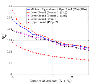
Following Proposition 6, let 𝑫𝒌+𝟏𝑪𝒌+𝟏1subscript𝑫𝒌1superscriptsubscript𝑪𝒌11\bm{D_{k+1}}\triangleq\bm{C_{k+1}}^{-1}. The minimax RNDOP (𝖱𝗑𝗒𝗓(+)(𝑫𝒌+𝟏)superscriptsubscript𝖱𝗑𝗒𝗓subscript𝑫𝒌1\mathsf{R}_{\mathsf{xyz}}^{(+)}(\bm{D_{k+1}})) after adding the (k+1)thsuperscript𝑘1th(k+1)^{\text{th}} anchor can be bounded using

1λ3(𝑪𝒌)+1λ2(𝑪𝒌)1subscript𝜆3subscript𝑪𝒌1subscript𝜆2subscript𝑪𝒌\displaystyle\tfrac{1}{\lambda_{3}(\bm{C_{k}})}+\tfrac{1}{\lambda_{2}(\bm{C_{k}})} 𝖱𝗑𝗒𝗓(+)(𝑫𝒌+𝟏)1λ2(𝑪𝒌)+1λ1(𝑪𝒌).absentsuperscriptsubscript𝖱𝗑𝗒𝗓subscript𝑫𝒌11subscript𝜆2subscript𝑪𝒌1subscript𝜆1subscript𝑪𝒌\displaystyle\leq\mathsf{R}_{\mathsf{xyz}}^{(+)}(\bm{D_{k+1}})\leq\tfrac{1}{\lambda_{2}(\bm{C_{k}})}+\tfrac{1}{\lambda_{1}(\bm{C_{k}})}. (37)
Proof.

We begin by noting that for the iterative anchor placement problem, (33a) can be written as 𝖱𝗑𝗒𝗓(+)(𝑫𝒌+𝟏)=λ3(𝑫𝒌+𝟏)+λ2(𝑫𝒌+𝟏)superscriptsubscript𝖱𝗑𝗒𝗓subscript𝑫𝒌1subscript𝜆3subscript𝑫𝒌1subscript𝜆2subscript𝑫𝒌1\mathsf{R}_{\mathsf{xyz}}^{(+)}(\bm{D_{k+1}})=\lambda_{3}(\bm{D_{k+1}})+\lambda_{2}(\bm{D_{k+1}}). Using this, the desired result follows from the direct application of Proposition 3 on the eigenvalues of 𝑪𝒌+𝟏subscript𝑪𝒌1\bm{C_{k+1}} using (36), and noting that λ4i(𝑪𝒌+𝟏)=λi1(𝑫𝒌+𝟏)subscript𝜆4𝑖subscript𝑪𝒌1subscriptsuperscript𝜆1𝑖subscript𝑫𝒌1\lambda_{4-i}(\bm{C_{k+1}})=\lambda^{-1}_{i}(\bm{D_{k+1}}) for i=1,2,3𝑖123i=1,2,3. ∎

Using (36), we transform (33a)-(33e) in the following main result to design an efficient minimax DOP-optimal single anchor placement scheme.

Lemma 4.

Let the anchor locations 𝒓𝒊,i=1,2,,kformulae-sequencesubscript𝒓𝒊𝑖12𝑘\bm{r_{i}},i=1,2,\cdots,k satisfy (33b)-(33e), where 𝑪𝒌=i=1k𝒓𝒊𝒓𝒊Tsubscript𝑪𝒌superscriptsubscript𝑖1𝑘subscript𝒓𝒊superscriptsubscript𝒓𝒊𝑇\bm{C_{k}}=\sum_{i=1}^{k}\bm{r_{i}}\bm{r_{i}}^{T}. The RNDOP-optimal anchor coordinate 𝒓𝒌+𝟏,𝟑𝑫(𝐫𝐧𝐝)subscriptsuperscript𝒓𝐫𝐧𝐝𝒌13𝑫\bm{r^{(\rm rnd)}_{k+1,3D}} in the current LCS is given by

𝒓𝒌+𝟏,𝟑𝑫(𝐫𝐧𝐝)=subscriptsuperscript𝒓𝐫𝐧𝐝𝒌13𝑫absent\displaystyle\bm{r^{(\rm rnd)}_{k+1,3D}}=\ argmin𝒓{tr([𝑪𝒌+(11k+1)𝒓𝒓T]1)\displaystyle\underset{\bm{r}}{{\rm arg}\min}\ \Big{\{}{\rm tr}\big{(}\big{[}\bm{C_{k}}+\big{(}1-\tfrac{1}{k+1}\big{)}\bm{rr}^{T}\big{]}^{-1}\big{)}-
λ([𝑪𝒌+(11k+1)𝒓𝒓T]1)}\displaystyle\lambda_{-}\big{(}\big{[}\bm{C_{k}}+\big{(}1-\tfrac{1}{k+1}\big{)}\bm{rr}^{T}\big{]}^{-1}\big{)}\Big{\}} (38a)
s.t.formulae-sequencest\displaystyle{\rm s.t.} 𝒓𝒍𝒓𝒓𝒖precedes-or-equalssubscript𝒓𝒍𝒓precedes-or-equalssubscript𝒓𝒖\displaystyle\ \bm{r_{l}}\preceq\bm{r}\preceq\bm{r_{u}} (38b)
𝒓𝒓𝒊2dth,i=1,2,,k.formulae-sequencesubscriptnorm𝒓subscript𝒓𝒊2subscript𝑑th𝑖12𝑘\displaystyle\|\bm{r}-\bm{r_{i}}\|_{2}\geq d_{\rm th},i=1,2,\cdots,k. (38c)
Proof.

The cost function is obtained by direct substitution of (36) in (33a). Since 𝑪𝒌+𝟏subscript𝑪𝒌1\bm{C_{k+1}} results from a rank-1 update applied to 𝑪𝒌𝟎succeedssubscript𝑪𝒌0\bm{C_{k}}\succ\bm{0}, it follows that 𝑪𝒌+𝟏𝟎succeedssubscript𝑪𝒌10\bm{C_{k+1}}\succ\bm{0}. In addition, as discussed in Proposition 6, the constraint (33e) is implicitly enforced by the update equation without translating the current LCS. Since the k𝑘k anchors already satisfy (33b)-(33c), they need to be enforced only for the (k+1)thsuperscript𝑘1th(k+1)^{\text{th}} anchor. Hence, proved. ∎

It is important to note that at the beginning of each iteration, the anchor centroid should be at 𝟎0\bm{0}. This needs to be facilitated by a coordinate translation of all anchors at the end of each iteration, as discussed later in Section VI.

IV-C Heuristic Cost Functions for Single Anchor Addition for 3D Positioning

IV-C1 Trace-based Heuristic

By observing the cost function (38) and its bounds in (37), it is clear that minimizing tr(𝑫𝒌+𝟏)tr([𝑪𝒌+(11k+1)𝒓𝒓T]1)trsubscript𝑫𝒌1trsuperscriptdelimited-[]subscript𝑪𝒌11𝑘1𝒓superscript𝒓𝑇1{\rm tr}(\bm{D_{k+1}})\triangleq{\rm tr}\big{(}\big{[}\bm{C_{k}}+\big{(}1-\tfrac{1}{k+1}\big{)}\bm{rr}^{T}\big{]}^{-1}\big{)} tends to minimize the maximum 3D RNDOP. Hence, we propose the trace-based minimization problem below.

Lemma 5.

Let the anchor locations 𝒓𝒊,i=1,2,,kformulae-sequencesubscript𝒓𝒊𝑖12𝑘\bm{r_{i}},i=1,2,\cdots,k satisfy (33b)-(33e), where 𝑪𝒌=i=1k𝒓𝒊𝒓𝒊Tsubscript𝑪𝒌superscriptsubscript𝑖1𝑘subscript𝒓𝒊superscriptsubscript𝒓𝒊𝑇\bm{C_{k}}=\sum_{i=1}^{k}\bm{r_{i}}\bm{r_{i}}^{T}. The trace-based heuristic RNDOP minimization problem is given by

𝒓𝒌+𝟏,𝟑𝑫(𝐭𝐫)subscriptsuperscript𝒓𝐭𝐫𝒌13𝑫\displaystyle\bm{r^{(\rm tr)}_{k+1,3D}} =argmax𝒓𝒓T𝑫𝒌+𝟏2𝒓1+kk+1𝒓T𝑫𝒌+𝟏𝒓absent𝒓argsuperscript𝒓𝑇superscriptsubscript𝑫𝒌12𝒓1𝑘𝑘1superscript𝒓𝑇subscript𝑫𝒌1𝒓\displaystyle=\underset{\bm{r}}{{\rm arg}\max}\ \tfrac{\bm{r}^{T}\bm{D_{k+1}}^{2}\bm{r}}{1+\frac{k}{k+1}\bm{r}^{T}\bm{D_{k+1}}\bm{r}}
s.t.formulae-sequencest\displaystyle{\rm s.t.} (38b)-(38c). (39)
Proof.

Applying Proposition 1 to 𝑫𝒌+𝟏𝑪𝒌+𝟏1subscript𝑫𝒌1superscriptsubscript𝑪𝒌11\bm{D_{k+1}}\triangleq\bm{C_{k+1}}^{-1} using (36), we get 𝑫𝒌+𝟏=𝑫𝒌kk+1𝑫𝒌𝒓𝒓T𝑫𝒌1+kk+1𝒓T𝑫𝒌𝒓subscript𝑫𝒌1subscript𝑫𝒌𝑘𝑘1subscript𝑫𝒌𝒓superscript𝒓𝑇subscript𝑫𝒌1𝑘𝑘1superscript𝒓𝑇subscript𝑫𝒌𝒓\bm{D_{k+1}}=\bm{D_{k}}-\frac{k}{k+1}\cdot\frac{\bm{D_{k}rr}^{T}\bm{D_{k}}}{1+\frac{k}{k+1}\bm{r}^{T}\bm{D_{k}r}}. Using properties of the trace and ignoring the terms independent of 𝒓𝒓\bm{r}, we get (5). The constraints remain unchanged relative to (38)-(38c). ∎

Remark 4.

When sequentially adding anchors based on the minimax RNDOP cost function over multiple iterations, the trace-based heuristic (5) tends to minimize all the eigenvalues of 𝑪𝒌+𝟏subscript𝑪𝒌1\bm{C_{k+1}} relative to those of 𝑪𝒌subscript𝑪𝒌\bm{C_{k}}. In other words, minimizing the trace in the (k+1)thsuperscript𝑘1th(k+1)^{\text{th}} iteration has the effect of tightening the upper and lower bounds in (37), thereby minimizing the maximum 3D RNDOP over consecutive iterations.

IV-C2 Eigenvector-based Heuristic

From (37), we observe that maximizing the minimum eigenvalue λ3(𝑪𝒌)subscript𝜆3subscript𝑪𝒌\lambda_{3}(\bm{C_{k}}) tends to minimize the upper bound. In the following, a computationally efficient heuristic scheme is proposed, which tends to minimize the maximum 3D RNDOP.

Lemma 6.

Let the anchor locations 𝒓𝒊,i=1,2,,kformulae-sequencesubscript𝒓𝒊𝑖12𝑘\bm{r_{i}},i=1,2,\cdots,k satisfy (33b)-(33e), where 𝑪𝒌=i=1k𝒓𝒊𝒓𝒊Tsubscript𝑪𝒌superscriptsubscript𝑖1𝑘subscript𝒓𝒊superscriptsubscript𝒓𝒊𝑇\bm{C_{k}}=\sum_{i=1}^{k}\bm{r_{i}}\bm{r_{i}}^{T}. The eigenvector-based heuristic-based optimization problem is given by

𝒓𝒌+𝟏,𝟑𝑫(𝐞𝐢𝐠)subscriptsuperscript𝒓𝐞𝐢𝐠𝒌13𝑫\displaystyle\bm{r^{(\rm eig)}_{k+1,3D}} =αmax𝒗(𝑪𝒌), whereabsentsubscript𝛼maxsubscript𝒗subscript𝑪𝒌 where\displaystyle=\alpha_{\rm max}\bm{v_{-}}(\bm{C_{k}}),\text{ where } (40a)
αmaxsubscript𝛼max\displaystyle\alpha_{\rm max} =argmax𝒓𝒍α𝒗(𝑪𝒌)𝒓𝒖α.absentprecedes-or-equalssubscript𝒓𝒍𝛼subscript𝒗subscript𝑪𝒌precedes-or-equalssubscript𝒓𝒖arg𝛼\displaystyle=\underset{\bm{r_{l}}\preceq\alpha\bm{v_{-}}(\bm{C_{k}})\preceq\bm{r_{u}}}{{\rm arg}\max}\ \alpha. (40b)
Proof.

We have 𝑪𝒌=i=13λi(𝑪𝒌)𝒗𝒊(𝑪𝒌)𝒗𝒊T(𝑪𝒌)subscript𝑪𝒌superscriptsubscript𝑖13subscript𝜆𝑖subscript𝑪𝒌subscript𝒗𝒊subscript𝑪𝒌subscriptsuperscript𝒗𝑇𝒊subscript𝑪𝒌\bm{C_{k}}=\sum_{i=1}^{3}\lambda_{i}(\bm{C_{k}})\bm{v_{i}}(\bm{C_{k}})\bm{v}^{T}_{\bm{i}}(\bm{C_{k}}). Substituting this in (36), if 𝒓=α𝒗𝟏(𝑪𝒌)=α𝒗(𝑪𝒌)𝒓𝛼subscript𝒗1subscript𝑪𝒌𝛼subscript𝒗subscript𝑪𝒌\bm{r}=\alpha\bm{v_{1}}(\bm{C_{k}})=\alpha\bm{v_{-}}(\bm{C_{k}}), then λi(𝑪𝒌+𝟏)subscript𝜆𝑖subscript𝑪𝒌1\lambda_{i}(\bm{C_{k+1}}) for i=1,2,3,𝑖123i=1,2,3, are given by λ1(𝑪𝒌+𝟏)=λ1(𝑪𝒌+𝟏)+kα2k+1subscript𝜆1subscript𝑪𝒌1subscript𝜆1subscript𝑪𝒌1𝑘superscript𝛼2𝑘1\lambda_{1}(\bm{C_{k+1}})=\lambda_{1}(\bm{C_{k+1}})+\tfrac{k\alpha^{2}}{k+1}, and λl(𝑪𝒌+𝟏)=λl(𝑪)subscript𝜆𝑙subscript𝑪𝒌1subscript𝜆𝑙𝑪\lambda_{l}(\bm{C_{k+1}})=\lambda_{l}(\bm{C}), for l=2,3𝑙23l=2,3. Therefore, maximizing α𝛼\alpha tends to minimize the upper bound in (37). Accounting for the box constraints, the maximum possible α𝛼\alpha (αmaxsubscript𝛼max\alpha_{\rm max}) is then obtained by solving (40b). ∎

It is worthwhile to note that (40a) is a convex problem that can be solved efficiently for large k𝑘k. However, the above formulation does not explicitly enforce the minimum distance constraint (38c). In Section VI, we discuss random perturbation-based methods to enforce (38c).

V RNDOP-Optimal Single Anchor Addition for 2D Positioning Outside the Convex Hull

In this section, we extend the results from Section IV to design single anchor addition schemes for beyond convex-hull 2D positioning. Intuitively, this extension is enabled by the fact that the key anchor-dependent quantities 𝑫𝑫\bm{D} (for 3D positioning) and 𝑬𝑬\bm{E} (for 2D positioning) are related by 𝑬=[𝑫]1:2,1:2𝑬subscriptdelimited-[]𝑫:121:2\bm{E}=[\bm{D}]_{1:2,1:2} as shown in Lemma 2. First, we first derive the update equation for the anchor matrix 𝑬𝑬\bm{E}, and introduce the notation used throughout the rest of this section.

Proposition 8.

Let the anchor locations 𝒓𝒊,i=1,2,,kformulae-sequencesubscript𝒓𝒊𝑖12𝑘\bm{r_{i}},i=1,2,\cdots,k, such that i=1k𝒓𝒊=𝟎superscriptsubscript𝑖1𝑘subscript𝒓𝒊0\sum_{i=1}^{k}\bm{r_{i}}=\bm{0}, 𝑬𝒌[𝑪𝒌1]1:2,1:2subscript𝑬𝒌subscriptdelimited-[]superscriptsubscript𝑪𝒌1:121:2\bm{E_{k}}\triangleq\big{[}\bm{C_{k}}^{-1}\big{]}_{1:2,1:2}, and 𝒓~[𝒓]1:2bold-~𝒓subscriptdelimited-[]𝒓:12\bm{\tilde{r}}\triangleq[\bm{r}]_{1:2}. Upon adding the (k+1)thsuperscript𝑘1th(k+1)^{\text{th}} anchor at 𝒓𝒌+𝟏subscript𝒓𝒌1\bm{r_{k+1}}, the updated anchor matrix 𝑬𝒌+𝟏subscript𝑬𝒌1\bm{E_{k+1}} is given by

𝑬𝒌+𝟏=𝑬𝒌(11k+1)𝑬𝒌𝒓~𝒌+𝟏𝒓~𝒌+𝟏T𝑬𝒌1+(11k+1)𝒓𝒌+𝟏T𝑫𝒌𝒓𝒌+𝟏.subscript𝑬𝒌1subscript𝑬𝒌11𝑘1subscript𝑬𝒌subscriptbold-~𝒓𝒌1superscriptsubscriptbold-~𝒓𝒌1𝑇subscript𝑬𝒌111𝑘1superscriptsubscript𝒓𝒌1𝑇subscript𝑫𝒌subscript𝒓𝒌1\displaystyle\bm{E_{k+1}}=\bm{E_{k}}-\tfrac{\big{(}1-\frac{1}{k+1}\big{)}\bm{E_{k}}\bm{\tilde{r}_{k+1}\tilde{r}_{k+1}}^{T}\bm{E_{k}}}{1+\big{(}1-\frac{1}{k+1}\big{)}\bm{r_{k+1}}^{T}\bm{D_{k}}\bm{r_{k+1}}}. (41)
Proof.

By definition, we have 𝑫𝒌+𝟏𝑪𝒌+𝟏1subscript𝑫𝒌1superscriptsubscript𝑪𝒌11\bm{D_{k+1}}\triangleq\bm{C_{k+1}}^{-1}. By applying Proposition 1 on (36), we get

𝑫𝒌+𝟏=𝑫𝒌(11k+1)𝑫𝒌𝒓𝒌+𝟏𝒓𝒌+𝟏T𝑫𝒌1+(11k+1)𝒓𝒌+𝟏T𝑫𝒌𝒓𝒌+𝟏.subscript𝑫𝒌1subscript𝑫𝒌11𝑘1subscript𝑫𝒌subscript𝒓𝒌1superscriptsubscript𝒓𝒌1𝑇subscript𝑫𝒌111𝑘1superscriptsubscript𝒓𝒌1𝑇subscript𝑫𝒌subscript𝒓𝒌1\displaystyle\bm{D_{k+1}}=\bm{D_{k}}-\tfrac{\big{(}1-\frac{1}{k+1}\big{)}\bm{D_{k}}\bm{r_{k+1}r_{k+1}}^{T}\bm{D_{k}}}{1+\big{(}1-\frac{1}{k+1}\big{)}\bm{r_{k+1}}^{T}\bm{D_{k}}\bm{r_{k+1}}}. (42)

Then, we use the definition 𝑬𝒍=[𝑫𝒍]1:2,1:2subscript𝑬𝒍subscriptdelimited-[]subscript𝑫𝒍:121:2\bm{E_{l}}=[\bm{D_{l}}]_{1:2,1:2} for l=k,k+1,𝑙𝑘𝑘1l=k,k+1, and the fact that

[𝑫𝒌𝒓𝒌+𝟏𝒓𝒌+𝟏T𝑫𝒌]1:2,1:2=𝑰𝟐×𝟑𝑫𝒌𝒓𝒌+𝟏𝒓𝒌+𝟏T𝑫𝒌𝑰𝟐×𝟑T,subscriptdelimited-[]subscript𝑫𝒌subscript𝒓𝒌1superscriptsubscript𝒓𝒌1𝑇subscript𝑫𝒌:121:2subscript𝑰23subscript𝑫𝒌subscript𝒓𝒌1superscriptsubscript𝒓𝒌1𝑇subscript𝑫𝒌superscriptsubscript𝑰23𝑇\displaystyle[\bm{D_{k}}\bm{r_{k+1}r_{k+1}}^{T}\bm{D_{k}}]_{1:2,1:2}=\bm{I_{2\times 3}}\bm{D_{k}}\bm{r_{k+1}r_{k+1}}^{T}\bm{D_{k}}\bm{I_{2\times 3}}^{T},

where 𝑰𝟐×𝟑=[𝑰𝟐 0𝟐×𝟏]subscript𝑰23delimited-[]subscript𝑰2subscript 021\bm{I_{2\times 3}}=[\bm{I_{2}}\ \ \bm{0_{2\times 1}}] and 𝟎𝟐×𝟏=[0 0]Tsubscript021superscriptdelimited-[]00𝑇\bm{0_{2\times 1}}=[0\ 0]^{T}. Simplifying the numerator of (42) using these, we get the desired result. ∎

The following result bounds the achievable 2D RNDOP when placing the (k+1)thsuperscript𝑘1th(k+1)^{\text{th}} anchor, given k𝑘k existing anchors.

Proposition 9.

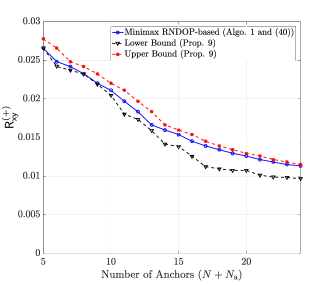
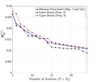
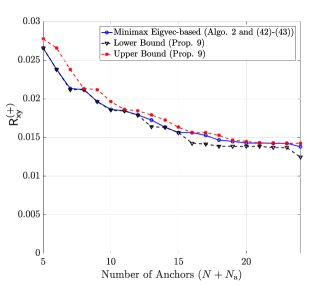
Let the current anchor matrix be 𝑬𝒌subscript𝑬𝒌\bm{E_{k}}. Then, the minimax 2D RNDOP for the (k+1)thsuperscript𝑘1th(k+1)^{\rm th} iteration can be bounded as λ(𝑬𝒌)𝖱𝗑𝗒(+)(𝑬𝒌+𝟏)λ+(𝑬𝒌)subscript𝜆subscript𝑬𝒌subscriptsuperscript𝖱𝗑𝗒subscript𝑬𝒌1subscript𝜆subscript𝑬𝒌\lambda_{-}(\bm{E_{k}})\leq\mathsf{R}^{(+)}_{\mathsf{xy}}(\bm{E_{k+1}})\leq\lambda_{+}(\bm{E_{k}}).

Proof.

The proof follows from the direct application of Proposition 3 on the eigenvalues of 𝑬𝒌subscript𝑬𝒌\bm{E_{k}} and 𝑬𝒌+𝟏subscript𝑬𝒌1\bm{E_{k+1}} in (41). ∎

Similar to Lemmas 4-6, we design single RNDOP-optimal anchor placement schemes for 2D positioning using (41) as shown below.

V-1 Iterative Minimax RNDOP-Optimal Anchor Addition for 2D Positioning

In the following result, we extend the iterative max-min RNDOP optimization problem discussed in Lemma 4 to the 2D positioning case.

Lemma 7.

The RNDOP-optimal anchor coordinate 𝒓𝒌+𝟏,𝟐𝑫(𝐫𝐧𝐝)subscriptsuperscript𝒓𝐫𝐧𝐝𝒌12𝑫\bm{r^{(\rm rnd)}_{k+1,2D}} in the (k+1)thsuperscript𝑘1th(k+1)^{\text{th}} iteration is given by solving

𝒓𝒌+𝟏,𝟐𝑫(𝐫𝐧𝐝)=subscriptsuperscript𝒓𝐫𝐧𝐝𝒌12𝑫absent\displaystyle\bm{r^{(\rm rnd)}_{k+1,2D}}= argmin𝒓λ+(𝑬𝒌(11k+1)𝑬𝒌𝒓~𝒓~T𝑬𝒌1+(11k+1)𝒓T𝑫𝒌𝒓)𝒓argsubscript𝜆subscript𝑬𝒌11𝑘1subscript𝑬𝒌bold-~𝒓superscriptbold-~𝒓𝑇subscript𝑬𝒌111𝑘1superscript𝒓𝑇subscript𝑫𝒌𝒓\displaystyle\underset{\bm{r}}{{\rm arg}\min}\ \lambda_{+}\Big{(}\bm{E_{k}}-\tfrac{\big{(}1-\frac{1}{k+1}\big{)}\bm{E_{k}}\bm{\tilde{r}\tilde{r}}^{T}\bm{E_{k}}}{1+\big{(}1-\frac{1}{k+1}\big{)}\bm{r}^{T}\bm{D_{k}}\bm{r}}\Big{)}
s.t.formulae-sequencest\displaystyle{\rm s.t.} (38b)(38c),𝒓~=[𝒓]1:2.38b38cbold-~𝒓subscriptdelimited-[]𝒓:12\displaystyle(\ref{eq:box_cnstrnt_no_trnsfrm})-(\ref{eq:dist_btwn_anch_cnstrnt_no_trnsfrm}),\bm{\tilde{r}}=[\bm{r}]_{1:2}. (43)
Proof.

The proof directly follows from Lemma 4, by noting that for 𝒁𝕊++2×2𝒁subscriptsuperscript𝕊22absent\bm{Z}\in\mathbb{S}^{2\times 2}_{++}, tr(𝒁)λ(𝒁)=λ+(𝒁)tr𝒁subscript𝜆𝒁subscript𝜆𝒁{\rm tr}(\bm{Z})-\lambda_{-}(\bm{Z})=\lambda_{+}(\bm{Z}). The constraints remain unchanged when compared to the optimal anchor placement schemes for 3D positioning. ∎

V-2 Trace-based Heuristic

Analyzing the cost function (7), it is evident that minimizing tr(𝑬𝒌+𝟏)trsubscript𝑬𝒌1{\rm tr}(\bm{E_{k+1}}) tends to minimize the max RNDOP. Hence, similar to the 3D case, we propose the trace-based RNDOP minimization problem below.

Lemma 8.

The trace-based heuristic 2D RNDOP minimization problem is given by

𝒓𝒌+𝟏,𝟑𝑫(𝐭𝐫)subscriptsuperscript𝒓𝐭𝐫𝒌13𝑫\displaystyle\bm{r^{(\rm tr)}_{k+1,3D}} =argmax𝒓𝒓~T𝑬𝒌2𝒓~1+(11k+1)𝒓T𝑫𝒌𝒓absent𝒓argsuperscriptbold-~𝒓𝑇superscriptsubscript𝑬𝒌2bold-~𝒓111𝑘1superscript𝒓𝑇subscript𝑫𝒌𝒓\displaystyle=\underset{\bm{r}}{{\rm arg}\max}\ \tfrac{\bm{\tilde{r}}^{T}\bm{E_{k}}^{2}\bm{\tilde{r}}}{1+\big{(}1-\frac{1}{k+1}\big{)}\bm{r}^{T}\bm{D_{k}}\bm{r}}
s.t.formulae-sequencest\displaystyle{\rm s.t.} (38b)(38c),𝒓~=[𝒓]1:2.38b38cbold-~𝒓subscriptdelimited-[]𝒓:12\displaystyle(\ref{eq:box_cnstrnt_no_trnsfrm})-(\ref{eq:dist_btwn_anch_cnstrnt_no_trnsfrm}),\bm{\tilde{r}}=[\bm{r}]_{1:2}. (44)
Proof.

In the cost function argmin𝒓tr(𝑬𝒌+𝟏)argsubscript𝒓trsubscript𝑬𝒌1{{\rm arg}\min}_{\bm{r}}\ \ {\rm tr}(\bm{E_{k+1}}), we observe from (41) that only the second term is dependent on 𝒓𝒓\bm{r}. Therefore, ignoring the first term, noticing that (11k+1)11𝑘1(1-\frac{1}{k+1}) in the numerator is independent of 𝒓𝒓\bm{r}, and absorbing the negative sign, we get the desired result. ∎

V-3 Eigenvector-based heuristic

This scheme finds the anchor location at the (k+1)thsuperscript𝑘1th(k+1)^{\rm th} iteration by solving two convex problems sequentially. The two problems are designed by observing in (41) that (a) aligning 𝒓~𝒌+𝟏subscriptbold-~𝒓𝒌1\bm{\tilde{r}_{k+1}} along the maximum eigenvector of 𝑬𝒌subscript𝑬𝒌\bm{E_{k}}, and (b) minimizing the denominator of the second term, tends to minimize λ+(𝑬𝒌+𝟏)subscript𝜆subscript𝑬𝒌1\lambda_{+}(\bm{E_{k+1}}). The mathematical formulation is provided in the following proposition.

Lemma 9.

The solution to the eigenvector heuristic-based 2D RNDOP minimization problem is given by 𝒓𝒌+𝟏,𝟐𝑫(𝐞𝐢𝐠)=[𝒓~𝝀+Trz]Tsubscriptsuperscript𝒓𝐞𝐢𝐠𝒌12𝑫superscriptdelimited-[]superscriptsubscriptbold-~𝒓limit-from𝝀𝑇subscript𝑟𝑧𝑇\bm{r^{(\rm eig)}_{k+1,2D}}=[\bm{\tilde{r}_{\lambda+}}^{T}\ r_{z}]^{T} where 𝒓~𝝀+=αmax𝒗+(𝑬𝒌)subscriptbold-~𝒓limit-from𝝀subscript𝛼maxsubscript𝒗subscript𝑬𝒌\bm{\tilde{r}_{\lambda+}}=\alpha_{\rm max}\bm{v}_{+}(\bm{E_{k}}) such that

P1:αmaxP1:subscript𝛼max\displaystyle\text{P1:}\ \ \alpha_{\rm max} =argmax[𝒓𝒍]1:2α𝒗+(𝑬𝒌)[𝒓𝒖]1:2α𝒗+(𝑬𝒌)absentprecedes-or-equalssubscriptdelimited-[]subscript𝒓𝒍:12𝛼subscript𝒗subscript𝑬𝒌precedes-or-equalssubscriptdelimited-[]subscript𝒓𝒖:12arg𝛼subscript𝒗subscript𝑬𝒌\displaystyle=\underset{[\bm{r_{l}}]_{1:2}\preceq\alpha\bm{v_{+}}(\bm{E_{k}})\preceq[\bm{r_{u}}]_{1:2}}{{\rm arg}\max}\ \ \alpha\bm{v}_{+}(\bm{E_{k}}) (45)
P2:rzP2:subscript𝑟𝑧\displaystyle\text{P2:}\ \ r_{z} =argmin𝒓𝒍]3z[𝒓𝒖]3pz2+2z𝒒T𝒓~𝝀+\displaystyle=\underset{\bm{r_{l}}]_{3}\leq z\leq[\bm{r_{u}}]_{3}}{{\rm arg}\min}\ \ pz^{2}+2z\bm{q}^{T}\bm{\tilde{r}_{\lambda+}} (46)

where 𝒒=[𝑫𝒌]1:2,3𝒒subscriptdelimited-[]subscript𝑫𝒌:123\bm{q}=[\bm{D_{k}}]_{1:2,3} and p=[𝑫𝒌]3,3𝑝subscriptdelimited-[]subscript𝑫𝒌33p=[\bm{D_{k}}]_{3,3}.

Proof.

The optimization problem (P1) seeks to minimize the numerator of the second term in (41) under the box constraints in (38b). (P1) is obtained in a similar manner as in Lemma 6 by noticing that (a) the minimum value of the numerator in the second term is achieved when 𝒓~=α𝒗+(𝑬𝒌)bold-~𝒓𝛼subscript𝒗subscript𝑬𝒌\bm{\tilde{r}}=\alpha\bm{v}_{+}(\bm{E_{k}}), and (b) α𝛼\alpha is chosen as high as possible under the XY-box constraints.

Then, (P2) solves for the z-coordinate by minimizing the denominator under (a) the box constraints for the z-coordinate, and (b) 𝒓~𝝀+subscriptbold-~𝒓limit-from𝝀\bm{\tilde{r}_{\lambda+}} which are the x- and y-coordinates of the (k+1)thsuperscript𝑘1th(k+1)^{\rm th} anchor. Considering the terms dependent on 𝒓𝒓\bm{r}, substituting 𝒓=[𝒓~𝝀+Trz]T𝒓superscriptdelimited-[]superscriptsubscriptbold-~𝒓limit-from𝝀𝑇subscript𝑟𝑧𝑇\bm{r}=[\bm{\tilde{r}_{\lambda+}}^{T}\ r_{z}]^{T}, and retaining only the terms dependent on the optimization variable rzsubscript𝑟𝑧r_{z}, we get the desired solution. ∎

It is worthwhile to note that in the above scheme, the distance constraint (38c) is not explicitly enforced. To do so, we use a random perturbation-based scheme analogous to Algorithm 2.

1:Input: method{𝚛𝚗𝚍,𝚝𝚛},mode{𝟸𝙳,𝟹𝙳},Na,dth,𝒓𝒖,𝒓𝒍formulae-sequencemethod𝚛𝚗𝚍𝚝𝚛mode2𝙳3𝙳subscript𝑁asubscript𝑑thsubscript𝒓𝒖subscript𝒓𝒍{\rm method}\in\{\mathtt{rnd},\mathtt{tr}\},{\rm mode}\in\{\mathtt{2D},\mathtt{3D}\},N_{\rm a},d_{\rm th},\bm{r_{u}},\bm{r_{l}}, a(N)={𝒓𝟏,𝒓𝟐,,𝒓𝑵}subscript𝑎𝑁subscript𝒓1subscript𝒓2subscript𝒓𝑵\mathcal{R}_{a}(N)=\{\bm{r_{1}},\bm{r_{2}},\cdots,\bm{r_{N}}\} such that constraints (33b)-(33e) are satisfied.
2:\triangleright Iteratively obtain coordinates of Nasubscript𝑁aN_{\rm a} anchors.
3:for k(N+1)𝑘𝑁1k\leftarrow(N+1) to (N+Na)𝑁subscript𝑁a(N+N_{\rm a}) do
4:    if k=(N+1)𝑘𝑁1k=(N+1) then\triangleright Initialization
5:         𝒓𝒖𝒓𝒖,𝒓𝒍𝒓𝒍formulae-sequencesubscriptsuperscript𝒓bold-′𝒖subscript𝒓𝒖subscriptsuperscript𝒓bold-′𝒍subscript𝒓𝒍\bm{r^{{}^{\prime}}_{u}}\leftarrow\bm{r_{u}},\bm{r^{{}^{\prime}}_{l}}\leftarrow\bm{r_{l}} \triangleright Save GCS box constraints
6:    end if
7:    𝑪𝒌𝟏i=1k1𝒓𝒊𝒓𝒊Tsubscript𝑪𝒌1superscriptsubscript𝑖1𝑘1subscript𝒓𝒊superscriptsubscript𝒓𝒊𝑇\bm{C_{k-1}}\leftarrow\sum_{i=1}^{k-1}\bm{r_{i}}\bm{r_{i}}^{T}
8:    𝑫𝒌𝟏𝑪𝒌𝟏1,𝑬𝒌𝟏[𝑫𝒌𝟏]1:2,1:2formulae-sequencesubscript𝑫𝒌1superscriptsubscript𝑪𝒌11subscript𝑬𝒌1subscriptdelimited-[]subscript𝑫𝒌1:121:2\bm{D_{k-1}}\leftarrow\bm{C_{k-1}}^{-1},\bm{E_{k-1}}\leftarrow[\bm{D_{k-1}}]_{1:2,1:2}
9:    if method=𝚛𝚗𝚍method𝚛𝚗𝚍{\rm method}=\mathtt{rnd} then
10:         if mode=𝟹𝙳mode3𝙳{\rm mode}=\mathtt{3D} then
11:             Solve (38)-(38c) to obtain 𝒓𝒌𝒓𝒌,𝟑𝑫(𝐫𝐧𝐝)subscript𝒓𝒌subscriptsuperscript𝒓𝐫𝐧𝐝𝒌3𝑫\bm{r_{k}}\leftarrow\bm{r^{(\rm rnd)}_{k,3D}}.
12:         else if mode=𝟸𝙳mode2𝙳{\rm mode}=\mathtt{2D} then
13:             Solve (7) to obtain 𝒓𝒌𝒓𝒌,𝟐𝑫(𝐫𝐧𝐝)subscript𝒓𝒌subscriptsuperscript𝒓𝐫𝐧𝐝𝒌2𝑫\bm{r_{k}}\leftarrow\bm{r^{(\rm rnd)}_{k,2D}}.
14:         end if
15:    else if method=𝚝𝚛method𝚝𝚛{\rm method}=\mathtt{tr} then
16:         if mode=𝟹𝙳mode3𝙳{\rm mode}=\mathtt{3D} then
17:             Solve (5) to obtain 𝒓𝒌𝒓𝒌,𝟑𝑫(𝐭𝐫)subscript𝒓𝒌subscriptsuperscript𝒓𝐭𝐫𝒌3𝑫\bm{r_{k}}\leftarrow\bm{r^{(\rm tr)}_{k,3D}}.
18:         else if mode=𝟸𝙳mode2𝙳{\rm mode}=\mathtt{2D} then
19:             Solve (8) to obtain 𝒓𝒌𝒓𝒌,𝟐𝑫(𝐭𝐫)subscript𝒓𝒌subscriptsuperscript𝒓𝐭𝐫𝒌2𝑫\bm{r_{k}}\leftarrow\bm{r^{(\rm tr)}_{k,2D}}.
20:         end if
Comment 5.
21:    else if method=𝚝𝚛method𝚝𝚛{\rm method}=\mathtt{tr} then
22:         Solve the optimization problem (40a).
23:         𝒓𝑵𝒓𝑵,𝟑𝑫(𝝀)subscriptsuperscript𝒓bold-′𝑵subscriptsuperscript𝒓subscript𝝀𝑵3𝑫\bm{r^{\prime}_{N}}\leftarrow\bm{r^{(\lambda_{-})}_{N,3D}}.
24:         𝒓𝑵Algorithm2(𝒓𝟏,,𝒓𝑵,dth)subscript𝒓𝑵Algorithm2subscript𝒓1subscriptsuperscript𝒓bold-′𝑵subscript𝑑th\bm{r_{N}}\leftarrow\text{Algorithm2}(\bm{r_{1}},\cdots,\bm{r^{\prime}_{N}},d_{\rm th}).
25:    end if
26:    \triangleright Compute new centroid and translate anchors/box constraints to new LCS.
27:    𝒓𝒄1ki=1k𝒓𝒊subscript𝒓𝒄1𝑘superscriptsubscript𝑖1𝑘subscript𝒓𝒊\bm{r_{c}}\leftarrow\frac{1}{k}\sum_{i=1}^{k}\bm{r_{i}}.
28:    𝒓𝒖(𝒓𝒖𝒓𝒄)subscript𝒓𝒖subscript𝒓𝒖subscript𝒓𝒄\bm{r_{u}}\leftarrow(\bm{r_{u}}-\bm{r_{c}}) and 𝒓𝒍(𝒓𝒍𝒓𝒄)subscript𝒓𝒍subscript𝒓𝒍subscript𝒓𝒄\bm{r_{l}}\leftarrow(\bm{r_{l}}-\bm{r_{c}}).
29:    for i1𝑖1i\leftarrow 1 to k𝑘k do
30:         𝒓𝒊(𝒓𝒊𝒓𝒄)subscript𝒓𝒊subscript𝒓𝒊subscript𝒓𝒄\bm{r_{i}}\leftarrow(\bm{r_{i}}-\bm{r_{c}})
31:    end for
32:    
33:    \triangleright Transform all coordinates back to GCS.
34:    𝒓𝒄(𝒓𝒖𝒓𝒖)subscriptsuperscript𝒓bold-′𝒄subscriptsuperscript𝒓bold-′𝒖subscript𝒓𝒖\bm{r^{\prime}_{c}}\leftarrow(\bm{r^{\prime}_{u}}-\bm{r_{u}}) \triangleright Equivalent to 𝒓𝒄(𝒓𝒍𝒓𝒍)subscriptsuperscript𝒓bold-′𝒄subscript𝒓𝒍subscriptsuperscript𝒓bold-′𝒍\bm{r^{\prime}_{c}}\leftarrow(\bm{r_{l}}-\bm{r^{\prime}_{l}})
35:    for i1𝑖1i\leftarrow 1 to (N+Na)𝑁subscript𝑁a(N+N_{\rm a}) do
36:         𝒓𝒊(𝒓𝒊+𝒓𝒄)subscript𝒓𝒊subscript𝒓𝒊subscriptsuperscript𝒓bold-′𝒄\bm{r_{i}}\leftarrow(\bm{r_{i}}+\bm{r^{\prime}_{c}})
37:    end for
38:    return a(N+Na)=a(N){𝒓𝑵+𝟏,,𝒓𝑵+𝑵𝐚}subscript𝑎𝑁subscript𝑁asubscript𝑎𝑁subscript𝒓𝑵1subscript𝒓𝑵subscript𝑵𝐚\mathcal{R}_{a}(N+N_{\rm a})=\mathcal{R}_{a}(N)\cup\{\bm{r_{N+1}},\cdots,\bm{r_{N+N_{\rm a}}}\}.
Algorithm 1 Iterative Minimax RNDOP and Trace Heuristic-based Anchor Placement for 2D and 3D Positioning

VI Iterative Anchor Addition Algorithms for 2D and 3D Positioning Outside the Convex Hull

In this section, we present an iterative anchor addition-based algorithmic framework for beyond convex hull positioning, that leverages the optimal single anchor addition schemes proposed in Sections IV and V. The goal is to adding Nasubscript𝑁aN_{\rm a} anchors to an existing set of N𝑁N anchors such that the maximum RNDOP is minimized, thereby resulting in robust error performance.

VI-A Algorithm Description

Algorithm 1 shows the iterative anchor addition algorithm for the minimax RNDOP and the trace-based heuristic schemes. Algorithm 2 shows the iterative anchor addition algorithm based on the eigenvector heuristic, coupled with a random perturbation step to ensure that the minimum anchor distance constraint is satisfied. Both the algorithms follow the sequence of steps outlined below. However for ease of exposition, we use Algorithm (1) to illustrate the key steps.

  1. 1.

    Initialization: The algorithm is initialized with N𝑁N anchor coordinates, constraint-related system parameters, and optimization method-related parameters. This corresponds to lines 1-2 in Algorithm 1.

  2. 2.

    Iterative Anchor Placement: Depending on the method, the appropriate single anchor addition problem is solved (lines 3-28 in Algorithm (1)). At each step, a coordinate translation is performed post anchor addition, to ensure that the anchor centroid is at the origin for the next iteration (lines 23-27 in Algorithm (1)); a necessary condition as highlighted in Remark 1.

  3. 3.

    Coordinate System Reversion: After all the Nasubscript𝑁aN_{\rm a} optimal anchor coordinates are computed in the LCS, they are transformed back to the global coordinate system for deployment purposes (lines 29-34 in Algorithm 1).

VI-B Random Perturbation-based Extension

The eigenvector heuristic-based schemes do not explicitly enforce the box and minimum anchor distance constraints. To do so, we propose a random perturbation-based extension shown in Algorithm 2, where we search for potential anchor locations near 𝒓𝒌,𝟑𝑫(𝐞𝐢𝐠)/𝒓𝒌,𝟐𝑫(𝐞𝐢𝐠)subscriptsuperscript𝒓𝐞𝐢𝐠𝒌3𝑫subscriptsuperscript𝒓𝐞𝐢𝐠𝒌2𝑫\bm{r^{(\rm eig)}_{k,3D}}/\bm{r^{(\rm eig)}_{k,2D}} (for 3D/2D positioning respectively) by randomly perturbing them until (38b)-(38c) is satisfied. This operation is repeated up to Nmaxsubscript𝑁maxN_{\rm max} times in each anchor addition iteration until the perturbed location satisfies all the constraints (lines 22-42 in Algorithm 2. However, the random perturbations are not guaranteed to yield a solution that satisfies all the constraints. To improve robustness, we propose adding redundant anchors. In this mechanism, if Nfsubscript𝑁fN_{\rm f} anchor addition iterations fail to yield a feasible anchor location, the algorithm effectively executes (Na+Nf)subscript𝑁asubscript𝑁f(N_{\rm a}+N_{\rm f}) iterations until a subset of Nasubscript𝑁aN_{\rm a} anchor locations satisfy (38b)-(38c).

1:Input: mode{𝟸𝙳,𝟹𝙳},dth,𝒓𝒖,𝒓𝒍,Na,η,Nmax,a(N)={𝒓𝟏,𝒓𝟐,,𝒓𝑵}formulae-sequencemode2𝙳3𝙳subscript𝑑thsubscript𝒓𝒖subscript𝒓𝒍subscript𝑁a𝜂subscript𝑁maxsubscript𝑎𝑁subscript𝒓1subscript𝒓2subscript𝒓𝑵{\rm mode}\in\{\mathtt{2D},\mathtt{3D}\},d_{\rm th},\bm{r_{u}},\bm{r_{l}},N_{\rm a},\eta,N_{\rm max},\mathcal{R}_{a}(N)=\{\bm{r_{1}},\bm{r_{2}},\cdots,\bm{r_{N}}\} such that constraints (33b)-(33e) are satisfied.
2:𝑽=𝟏𝑵{0,1}N𝑽subscript1𝑵superscript01𝑁\bm{V}=\bm{1_{N}}\in\{0,1\}^{N}, q0,n0formulae-sequence𝑞0𝑛0q\leftarrow 0,n\leftarrow 0.
3:while nNa𝑛subscript𝑁an\leq N_{\rm a} do
4:    qq+1,k(N+q)formulae-sequence𝑞𝑞1𝑘𝑁𝑞q\leftarrow q+1,k\leftarrow(N+q).
5:    if q=1𝑞1q=1 then
6:         𝒓𝒖𝒓𝒖,𝒓𝒍𝒓𝒍formulae-sequencesubscriptsuperscript𝒓bold-′𝒖subscript𝒓𝒖subscriptsuperscript𝒓bold-′𝒍subscript𝒓𝒍\bm{r^{{}^{\prime}}_{u}}\leftarrow\bm{r_{u}},\bm{r^{{}^{\prime}}_{l}}\leftarrow\bm{r_{l}} \triangleright Save GCS box constraints
7:    end if
8:    𝑪𝒌𝟏i=1k1𝒓𝒊𝒓𝒊Tsubscript𝑪𝒌1superscriptsubscript𝑖1𝑘1subscript𝒓𝒊superscriptsubscript𝒓𝒊𝑇\bm{C_{k-1}}\leftarrow\sum_{i=1}^{k-1}\bm{r_{i}}\bm{r_{i}}^{T}
9:    𝑫𝒌𝟏𝑪𝒌𝟏1,𝑬𝒌𝟏[𝑫𝒌𝟏]1:2,1:2formulae-sequencesubscript𝑫𝒌1superscriptsubscript𝑪𝒌11subscript𝑬𝒌1subscriptdelimited-[]subscript𝑫𝒌1:121:2\bm{D_{k-1}}\leftarrow\bm{C_{k-1}}^{-1},\bm{E_{k-1}}\leftarrow[\bm{D_{k-1}}]_{1:2,1:2}
10:    if mode=𝟹𝙳mode3𝙳{\rm mode}=\mathtt{3D} then
11:         Solve (40a)-(40b) to get 𝒓𝒓𝒌,𝟑𝑫(𝐞𝐢𝐠)superscript𝒓bold-‡subscriptsuperscript𝒓𝐞𝐢𝐠𝒌3𝑫\bm{r^{\ddagger}}\leftarrow\bm{r^{\rm(eig)}_{k,3D}}.
12:    else if mode=𝟸𝙳mode2𝙳{\rm mode}=\mathtt{2D} then
13:         Solve (45)-(46) to get 𝒓𝒓𝒌,𝟐𝑫(𝐞𝐢𝐠)superscript𝒓bold-‡subscriptsuperscript𝒓𝐞𝐢𝐠𝒌2𝑫\bm{r^{\ddagger}}\leftarrow\bm{r^{\rm(eig)}_{k,2D}}.
14:    end if
15:    for l1𝑙1l\leftarrow 1 to (k1)𝑘1(k-1) do
16:         dl𝒓𝒓𝒍2subscript𝑑𝑙subscriptnormsuperscript𝒓bold-‡subscript𝒓𝒍2d_{l}\leftarrow\|\bm{r^{\ddagger}}-\bm{r_{l}}\|_{2}
17:    end for
18:    dminmin([d1,d2,,dk1])subscript𝑑minsubscript𝑑1subscript𝑑2subscript𝑑𝑘1d_{\rm min}\leftarrow\min([d_{1},d_{2},\cdots,d_{k-1}])
19:    \triangleright If (38c) is satisfied, we have a new valid anchor location
20:    if dmindthsubscript𝑑minsubscript𝑑thd_{\rm min}\geq d_{\rm th} then
21:         𝒓𝒌𝒓,nn+1,𝑽(k)1formulae-sequencesubscript𝒓𝒌superscript𝒓bold-‡formulae-sequence𝑛𝑛1𝑽𝑘1\bm{r_{k}}\leftarrow\bm{r^{\ddagger}},n\leftarrow n+1,\bm{V}(k)\leftarrow 1.
22:    else\triangleright perform random perturbation until (38c) is satisfied
23:         𝒓𝒌𝒓,dmin,cdminformulae-sequencesubscript𝒓𝒌superscript𝒓bold-‡subscript𝑑mincsubscript𝑑min\bm{r_{k}}\leftarrow\bm{r^{\ddagger}},d_{\rm min,c}\leftarrow d_{\rm min} \triangleright Initialize 𝒓𝒌subscript𝒓𝒌\bm{r_{k}} and minimum anchor separation
24:         for p0𝑝0p\leftarrow 0 to Nmaxsubscript𝑁maxN_{\rm max} do
25:             θ𝒰[π,π],ϕ𝒰[π2,π2]formulae-sequencesimilar-to𝜃𝒰𝜋𝜋similar-toitalic-ϕ𝒰𝜋2𝜋2\theta\sim\mathcal{U}[-\pi,\pi],\phi\sim\mathcal{U}\big{[}-\tfrac{\pi}{2},\tfrac{\pi}{2}\big{]}
26:             𝒓=𝒓+ηdth𝒂(θ,ϕ)superscript𝒓bold-†superscript𝒓bold-‡𝜂subscript𝑑th𝒂𝜃italic-ϕ\bm{r^{\dagger}}=\bm{r^{\ddagger}}+\eta d_{\rm th}\cdot\bm{a}(\theta,\phi) \triangleright perturb 𝒓superscript𝒓bold-‡\bm{r^{\ddagger}} by a distance ηdth(η>1)𝜂subscript𝑑th𝜂1\eta d_{\rm th}\ (\eta>1) along a random direction (θ,ϕ)𝜃italic-ϕ(\theta,\phi).
27:             if 𝒓𝒍𝒓𝒓𝒖precedes-or-equalssubscript𝒓𝒍superscript𝒓bold-†precedes-or-equalssubscript𝒓𝒖\bm{r_{l}}\preccurlyeq\bm{r^{\dagger}}\preccurlyeq\bm{r_{u}} then
28:                 for j1𝑗1j\leftarrow 1 to (k1)𝑘1(k-1) do
29:                     dj𝒓𝒓𝒋2subscriptsuperscript𝑑𝑗subscriptnormsuperscript𝒓bold-†subscript𝒓𝒋2d^{\dagger}_{j}\leftarrow\|\bm{r^{\dagger}}-\bm{r_{j}}\|_{2}
30:                 end for
31:                 dmin=min([d1,d2,,dk1])subscript𝑑minsubscriptsuperscript𝑑1subscriptsuperscript𝑑2subscriptsuperscript𝑑𝑘1d_{\rm min}=\min([d^{\dagger}_{1},d^{\dagger}_{2},\cdots,d^{\dagger}_{k-1}])
32:                 if dmindthsubscript𝑑minsubscript𝑑thd_{\rm min}\geq d_{\rm th} then
33:                     𝒓𝒌𝒓,nn+1,𝑽(k)1formulae-sequencesubscript𝒓𝒌superscript𝒓bold-†formulae-sequence𝑛𝑛1𝑽𝑘1\bm{r_{k}}\leftarrow\bm{r^{\dagger}},n\leftarrow n+1,\bm{V}(k)\leftarrow 1.
34:                     break
35:                 else if dmin>dmin,csubscript𝑑minsubscript𝑑mincd_{\rm min}>d_{\rm min,c} then
36:                     𝒓𝒌𝒓,dmin,cdmin,𝑽(k)0formulae-sequencesubscript𝒓𝒌superscript𝒓bold-†formulae-sequencesubscript𝑑mincsubscript𝑑min𝑽𝑘0\bm{r_{k}}\leftarrow\bm{r^{\dagger}},d_{\rm min,c}\leftarrow d_{\rm min},\bm{V}(k)\leftarrow 0
37:                 end if
38:             else
39:                 continue
40:             end if
41:         end for
42:    end if
43:    Lines 14-18 in Algorithm 1.
Comment 6.
44:    𝒓𝒄1ki=1k𝒓𝒊subscript𝒓𝒄1𝑘superscriptsubscript𝑖1𝑘subscript𝒓𝒊\bm{r_{c}}\leftarrow\frac{1}{k}\sum_{i=1}^{k}\bm{r_{i}}.
45:    𝒓𝒖(𝒓𝒖𝒓𝒄)subscript𝒓𝒖subscript𝒓𝒖subscript𝒓𝒄\bm{r_{u}}\leftarrow(\bm{r_{u}}-\bm{r_{c}}) and 𝒓𝒍(𝒓𝒍𝒓𝒄)subscript𝒓𝒍subscript𝒓𝒍subscript𝒓𝒄\bm{r_{l}}\leftarrow(\bm{r_{l}}-\bm{r_{c}}).
46:    for i1𝑖1i\leftarrow 1 to N𝑁N do
47:         𝒓𝒊(𝒓𝒊𝒓𝒄)subscript𝒓𝒊subscript𝒓𝒊subscript𝒓𝒄\bm{r_{i}}\leftarrow(\bm{r_{i}}-\bm{r_{c}})
48:    end for sss
49:    end while
50:    𝒓𝒄(𝒓𝒖𝒓𝒖)=(𝒓𝒍𝒓𝒍)subscriptsuperscript𝒓bold-′𝒄subscriptsuperscript𝒓bold-′𝒖subscript𝒓𝒖subscript𝒓𝒍subscriptsuperscript𝒓bold-′𝒍\bm{r^{\prime}_{c}}\leftarrow(\bm{r^{\prime}_{u}}-\bm{r_{u}})=(\bm{r_{l}}-\bm{r^{\prime}_{l}})
51:    val=subscriptval\mathcal{R}_{\rm val}=\emptyset.
52:    for i1𝑖1i\leftarrow 1 to k𝑘k do
53:         𝒓𝒊(𝒓𝒊+𝒓𝒄)subscript𝒓𝒊subscript𝒓𝒊subscriptsuperscript𝒓bold-′𝒄\bm{r_{i}}\leftarrow(\bm{r_{i}}+\bm{r^{\prime}_{c}}) \triangleright Transform all anchor coordinates to GCS.
54:         if 𝑽(i)=1𝑽𝑖1\bm{V}(i)=1 then
55:             valval{𝒓𝒊}subscriptvalsubscriptvalsubscript𝒓𝒊\mathcal{R}_{\rm val}\leftarrow\mathcal{R}_{\rm val}\cup\{\bm{r_{i}}\}.
56:         end if
57:    end for
58:    return a(N+Na)=a(N)valsubscript𝑎𝑁subscript𝑁asubscript𝑎𝑁subscriptval\mathcal{R}_{a}(N+N_{\rm a})=\mathcal{R}_{a}(N)\cup\mathcal{R}_{\rm val}.
Algorithm 2 Iterative Eigenvector Heursitic-based Iterative Anchor Placement for 2D and 3D Positioning

VI-C Computational Complexity and Convergence

VI-C1 Algorithm 1

Since the considered optimization problems are non-convex, convergence to the global minima cannot be guaranteed. A rigorous proof of convergence to a local minima is beyond the scope of this work. However, we would like to emphasize that we use the Primal-Dual Interior-Point (PDIP) class of algorithms such as [37] based on the trust-region and line search-based approaches, which have robust convergence properties that ensure that each step makes progress towards a local minima [37].

Let d𝑑d be the dimension in which the target is tracked. Hence, d=2𝑑2d=2 and 333 for 2D and 3D positioning respectively. Since the optimization problems composed of Algorithm 1 are nonlinear and non-convex, we solve them using PDIP-based methods. Here, the Newon step is the limiting operation requiring the most number of computations, and the corresponding worst-case complexity is O(d3)𝑂superscript𝑑3O(d^{3}). In addition, the complexity of the cost function computation for each single anchor addition problem is no greater than O(d3)𝑂superscript𝑑3O(d^{3}), since they are based on operations such as the eigen-decomposition, multiplication, and inversion of 𝕊d×dsuperscript𝕊𝑑𝑑\mathbb{S}^{d\times d} matrices [38]. For adding the kthsuperscript𝑘thk^{\rm th} anchor, an ϵitalic-ϵ\epsilon-accurate iteration can be computed in O(klog(1ϵ))𝑂𝑘1italic-ϵO\big{(}\sqrt{k}\log\big{(}\frac{1}{\epsilon}\big{)}\big{)} steps [39], [40], [30]. Therefore, a single sequential anchor addition step in Algorithm 1 has a complexity of O(d3klog(1ϵ))𝑂superscript𝑑3𝑘1italic-ϵO\big{(}d^{3}\sqrt{k}\log\big{(}\frac{1}{\epsilon}\big{)}\big{)}. Therefore, to add Nasubscript𝑁𝑎N_{a} anchors sequentially to N𝑁N existing anchors, the computational complexity is n=NN+Na1O(d3nlog(1ϵ))superscriptsubscript𝑛𝑁𝑁subscript𝑁𝑎1𝑂superscript𝑑3𝑛1italic-ϵ\sum_{n=N}^{N+N_{a}-1}O\big{(}d^{3}\sqrt{n}\log\big{(}\frac{1}{\epsilon}\big{)}\big{)}. Using the fact that i=1xi1/2(i=1xi)1/2subscript𝑖1subscriptsuperscript𝑥12𝑖superscriptsubscript𝑖1subscript𝑥𝑖12\sum_{i=1}x^{1/2}_{i}\leq\big{(}\sum_{i=1}x_{i}\big{)}^{1/2}, the computational complexity can be simplified as O(d3N1+Na(Na+1)2log(1ϵ))𝑂superscript𝑑3𝑁1subscript𝑁𝑎subscript𝑁𝑎121italic-ϵO\Big{(}d^{3}\sqrt{N-1+\frac{N_{a}(N_{a}+1)}{2}}\log\big{(}\frac{1}{\epsilon}\big{)}\Big{)}. If NaNmuch-greater-thansubscript𝑁𝑎𝑁N_{a}\gg N, then the worst-case complexity can be accurately approximated using O(d3Nalog(1ϵ))𝑂superscript𝑑3subscript𝑁𝑎1italic-ϵO\big{(}d^{3}N_{a}\log\big{(}\frac{1}{\epsilon}\big{)}\big{)}.

VI-C2 Algorithm 2

Due to the random perturbation step, convergence is not guaranteed for each iteration of the anchor addition scheme. As discussed in Section VI-B, this is alleviated by retaining the constraint-violating anchor locations and proceeding forward to add redundant additional anchors until a total of Nasubscript𝑁aN_{\rm a} constraint-satisfying anchor locations are found, and then removing the anchors that violate the deployment constraints. The number of removed anchors (Nfsubscript𝑁fN_{\rm f}) depends on the optimization problem parameters 𝒓𝒖,𝒓𝒍,dthsubscript𝒓𝒖subscript𝒓𝒍subscript𝑑th\bm{r_{u}},\bm{r_{l}},d_{\rm th}, and Nasubscript𝑁aN_{\rm a}. A rigorous analysis of the parameters’ impact on the convergence is out of the scope of this paper, and will be addressed in a future work. Nevertheless, we have comprehensively analyzed the execution time performance of Algorithm 2 using Monte-Carlo simulations in Section VII.

The computational complexity is determined by two key steps: (a) Eigen-decomposition of 𝑫𝑫\bm{D}, which is given by O(d3)𝑂superscript𝑑3O(d^{3}), and (b) the random perturbation and minimum anchor distance comparison step, which has a complexity of O(kNmax)𝑂𝑘subscript𝑁maxO(kN_{\rm max}) for adding the (k+1)thsuperscript𝑘1th(k+1)^{\rm th} anchor. Therefore, the worst-case complexity for Algorithm 2 is given by O((Na+Nf)d3+(N+i=1Na+Nfi)Nmax)𝑂subscript𝑁asubscript𝑁fsuperscript𝑑3𝑁superscriptsubscript𝑖1subscript𝑁asubscript𝑁f𝑖subscript𝑁maxO\big{(}(N_{\rm a}+N_{\rm f})d^{3}+(N+\sum_{i=1}^{N_{\rm a}+N_{\rm f}}i)N_{\rm max}\big{)}. If (Na+Nf)NN_{\rm a}+N_{\rm f})\gg N, this simplifies to O((Na+Nf)d3+(Na+Nf)2Nmax)𝑂subscript𝑁asubscript𝑁fsuperscript𝑑3superscriptsubscript𝑁asubscript𝑁f2subscript𝑁maxO\big{(}(N_{\rm a}+N_{\rm f})d^{3}+(N_{\rm a}+N_{\rm f})^{2}N_{\rm max}\big{)}.

Refer to caption
(a)
Refer to caption
(b)
Refer to caption
(c)
Figure 3: Variation of 𝖱𝗑𝗒𝗓(+)subscriptsuperscript𝖱𝗑𝗒𝗓{\mathsf{R}^{(+)}_{\mathsf{xyz}}} and its bounds as a function of the number of total anchors (M=N+Na𝑀𝑁subscript𝑁aM=N+N_{\rm a}) under the (a) Minimax RNDOP-optimal scheme (Lemma 4), (b) Minimax Trace-based scheme (Lemma 5), and (c) Minimax Eigenvector-based scheme (Lemma 6), for beyond convex hull 3D localization.
Refer to caption
(a)
Refer to caption
(b)
Refer to caption
(c)
Figure 4: Variation of 𝖱𝗑𝗒(+)subscriptsuperscript𝖱𝗑𝗒{\mathsf{R}^{(+)}_{\mathsf{xy}}} and its bounds as a function of the number of anchors (M=N+Na𝑀𝑁subscript𝑁aM=N+N_{\rm a}) under the (a) Minimax RNDOP-optimal scheme (Lemma 7), (b) Minimax Trace-based scheme (Lemma 8), and (c) Minimax Eigenvector-based (Lemma 9) scheme, for 2D (XY) beyond convex hull localization.

VII Numerical Results

We consider a beyond convex hull localization scenario, as shown in Fig. 2. In the following subsections, we present numerical results to (a) verify the iterative upper and lower bounds, and (b) demonstrate the error and computational performance of our proposed iterative anchor placement algorithms in 2D and 3D localization scenarios.

VII-A Comparison of Maximum RNDOP Performance

Recall that for far-away targets outside the convex hull, a target with the maximum RNDOP tends to have the worst localization error on average when the range error statistics is similar for all targets. Here, we consider a UAV-based localization scenario, where the UAVs are constrained to be located in the box defined by 𝒓𝒍=[30 m,20 m,10 m]subscript𝒓𝒍30 m20 m10 m\bm{r_{l}}=[-30\text{ m},-20\text{ m},-10\text{ m}], and 𝒓𝒖=[30 m,20 m,10 m]subscript𝒓𝒖30 m20 m10 m\bm{r_{u}}=[30\text{ m},20\text{ m},10\text{ m}], and the minimum anchor separation distance dth=4.472subscript𝑑th4.472d_{\rm th}=4.472 m. Each scheme is initialized with N=4𝑁4N=4 anchors, whose locations are obtained using a Monte-Carlo method. Specifically, the initial anchor configuration is set to one that has the minimum 𝖱𝗑𝗒𝗓(+)subscriptsuperscript𝖱𝗑𝗒𝗓\mathsf{R}^{(+)}_{\mathsf{xyz}} (for 3D)/𝖱𝗑𝗒(+)subscriptsuperscript𝖱𝗑𝗒\mathsf{R}^{(+)}_{\mathsf{xy}} (for 2D) after 105superscript10510^{5} Monte-Carlo trials.

From Fig. 3, we observe that 𝖱𝗑𝗒𝗓(+)subscriptsuperscript𝖱𝗑𝗒𝗓\mathsf{R}^{(+)}_{\mathsf{xyz}} decreases sublinearly as a function of the total number of anchors (M𝑀M), for all the proposed anchor placement schemes. While the performance of the minimax RNDOP-optimal (Fig. 3(a)) and trace-based (Fig. 3(b)) schemes are close, the eigenvector-based scheme (Fig. 3(c)) has noticeably higher 𝖱𝗑𝗒𝗓(+)subscriptsuperscript𝖱𝗑𝗒𝗓\mathsf{R}^{(+)}_{\mathsf{xyz}}. For the considered scenario, the minimax RNDOP and trace-based iterative schemes yield similar 𝖱𝗑𝗒𝗓(+)subscriptsuperscript𝖱𝗑𝗒𝗓\mathsf{R}^{(+)}_{\mathsf{xyz}} performance since λ1(𝑫𝒌)i={2,3}λi(𝑫𝒌)much-less-thansubscript𝜆1subscript𝑫𝒌subscript𝑖23subscript𝜆𝑖subscript𝑫𝒌\lambda_{1}(\bm{D_{k}})\ll\sum_{i=\{2,3\}}\lambda_{i}(\bm{D_{k}}) at initialization, and holds true as the anchor index k𝑘k increases. It is worthwhile to point out that the trace-based scheme slightly outperforms its minimax RNDOP counterpart. This is because it minimizes the sum of all the eigenvalues, unlike the minimax RNDOP scheme which minimizes the sum of the two largest eigenvalues. For instance, since the RNDOP-based scheme incentivizes minimization of the top two eigenvalues at each iteration, the minimum eigenvalue risks remaining stagnant over multiple iterations, eventually ending up becoming the largest, or second-largest eigenvalue. In other words, accounting for all eigenvalues during iterative minimization makes the scheme more robust against eigenvalue ordering changes that occur over multiple iterations.

On the other hand, the resultant 𝖱𝗑𝗒𝗓(+)subscriptsuperscript𝖱𝗑𝗒𝗓\mathsf{R}^{(+)}_{\mathsf{xyz}} is relatively large for the eigenvector-based heuristic scheme since it sequentially minimizes the numerator and maximizes the denominator of the trace-based heuristic, rather than minimizing the fractional term jointly. However, the random perturbation step introduces stochasticity into the RNDOP performance which is non-trivial to analyze from a theoretical standpoint. Nevertheless, the minimax RNDOP is 2030%20percent3020-30\% higher when compared to the other two schemes. Next, we observe that the iterative upper and lower bounds in (37) are fairly tight for all the schemes. Finally, the universal lower bound (34b) is quite loose, whereas the tightness of its trace-based variant (34a) is similar to that of (37). This is consistent due to the fact that (34b) is itself a lower bound on (34a).

From Fig. 4, we observe that the trace-based scheme outperforms the other two methods in terms of 𝖱𝗑𝗒(+)subscriptsuperscript𝖱𝗑𝗒\mathsf{R}^{(+)}_{\mathsf{xy}}. The 𝖱𝗑𝗒(+)subscriptsuperscript𝖱𝗑𝗒\mathsf{R}^{(+)}_{\mathsf{xy}} performance of the trace-based iterative scheme is superior when compared to the other. This can also be attributed to the ‘long-term RNDOP minimization behavior’ of trace-based cost functions outlined in the previous few paragraphs. Furthermore, we observe that the iterative upper and lower bounds (Proposition 9) is tight for all the proposed 2D-optimal anchor placement schemes.
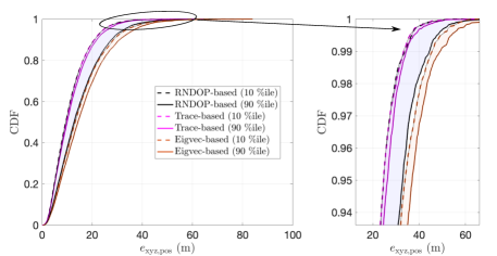
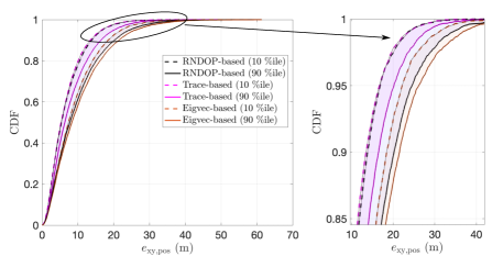
Refer to caption
(a)
Refer to caption
(b)
Figure 5: (a) CDF of 3D positioning error for the i10subscriptsubscript𝑖10\mathcal{R}_{i_{10}} (good, denoted by dashed lines) and i90subscriptsubscript𝑖90\mathcal{R}_{i_{90}} (bad, denoted by solid lines) anchor configurations obtained by each iterative method (3D optimal schemes), for targets distributed uniformly at random in a sphere of radius 200m. (b) CDF of 2D positioning error for the i10subscriptsubscript𝑖10\mathcal{R}_{i_{10}} (good, denoted by dashed lines) and i90subscriptsubscript𝑖90\mathcal{R}_{i_{90}} (bad, denoted by solid lines) anchor configurations obtained by each iterative method (2D optimal schemes), for targets distributed uniformly on the XY-plane at random in a circle of radius 200m.

VII-B Comparison of 3D and 2D Localization Error

To compare the 3D/2D localization error performance of the proposed methods, we performed Nmc,algo=500subscript𝑁mcalgo500N_{\rm mc,algo}=500 Monte-Carlo (MC) simulations for each iterative anchor placement scheme. The following steps are undertaken in each MC trial.

VII-B1 Initialization

The initial Nanchor𝑁anchorN-\text{anchor} configuration is obtained using Nmc,init=105subscript𝑁mcinitsuperscript105N_{\rm mc,init}=10^{5} trials. In each trial, N=4𝑁4N=4 anchors are placed uniformly at random in the box specified by 𝒓𝒍subscript𝒓𝒍\bm{r_{l}} and 𝒓𝒖subscript𝒓𝒖\bm{r_{u}}. The initial anchor configuration corresponds to the one that (a) satisfies the minimum anchor separation (dthsubscript𝑑thd_{\rm th}) constraint and (b) has the lowest 𝖱𝗑𝗒𝗓(+)subscriptsuperscript𝖱𝗑𝗒𝗓\mathsf{R}^{(+)}_{\mathsf{xyz}} (for 3D localization) or 𝖱𝗑𝗒(+)subscriptsuperscript𝖱𝗑𝗒\mathsf{R}^{(+)}_{\mathsf{xy}} (for 2D localization).

VII-B2 Iterative Anchor Placement

For each MC trial, the proposed iterative anchor placement methods are executed using Algorithm 1 (for the Minimax RNDOP and the Trace-based heuristic methods) and Algorithm 2 (for the Eigenvector heuristic-based scheme) to add Na=20subscript𝑁a20N_{\rm a}=20 additional anchors to the initial N=4𝑁4N=4 anchors in the network.

Configuration Selection

For characterizing the error performance of each method, we choose two anchor configurations per method: one configuration that corresponds to low max-RNDOP (low localization error), and another that corresponds to high max-RNDOP (high localization error). Let the max-RNDOP of the anchor configuraton obtained in all the Nmc,algosubscript𝑁mcalgoN_{\rm mc,algo} MC trials be ordered in descending order as 𝖱1(+)𝖱2(+)𝖱Nmc,algo(+)subscriptsuperscript𝖱1subscriptsuperscript𝖱2subscriptsuperscript𝖱subscript𝑁mcalgo\mathsf{R}^{(+)}_{1}\leq\mathsf{R}^{(+)}_{2}\leq\cdots\leq\mathsf{R}^{(+)}_{N_{\rm mc,algo}}, such that the corresponding anchor configuration is i,i=1,2,,Nmc,algoformulae-sequencesubscript𝑖𝑖12subscript𝑁mcalgo\mathcal{R}_{i},i=1,2,\cdots,N_{\rm mc,algo}. The “good” anchor configuration is chosen to correspond to the 10-percentile max-RNDOP (i.e. 𝖱i10(+)subscriptsuperscript𝖱subscript𝑖10\mathsf{R}^{(+)}_{i_{10}}, where i10=0.1×Nmc,algosubscript𝑖100.1subscript𝑁mcalgoi_{10}=\lfloor 0.1\times N_{\rm mc,algo}\rfloor), and the “bad” anchor configuration corresponds to the 90-percentile max-RNDOP (i.e. 𝖱i90(+)subscriptsuperscript𝖱subscript𝑖90\mathsf{R}^{(+)}_{i_{90}}, where i90=0.9×Nmc,algosubscript𝑖900.9subscript𝑁mcalgoi_{90}=\lceil 0.9\times N_{\rm mc,algo}\rceil).

Random Target Deployment

To evaluate the efficacy of the good and bad anchor configurations under investigation, Ntarg=104subscript𝑁targsuperscript104N_{\rm targ}=10^{4} targets are placed in the network.

  1. 1.

    3D Localization: For evaluating the 3D localization performance, each target is placed uniformly at random in a sphere of radius rcov=200subscript𝑟cov200r_{\rm cov}=200 m centered at the origin.

  2. 2.

    2D Localization: For evaluating the 2D localization performance, each target is placed uniformly at random in a circle of radius rcov=200subscript𝑟cov200r_{\rm cov}=200 m on the XY plane centered at the origin.

Note that even though we are concerned with beyond convex-hull localization scenarios, we relax this constraint for evaluation purposes and consider the localization error performance across all possible target locations within the spherical/circular coverage region for 3D/2D localization respectively.

Localization using NLS

The target performs N+Na=24𝑁subscript𝑁a24N+N_{\rm a}=24 ToA-based range measurements using the relation r^i=max(0,ri+wi)subscript^𝑟𝑖0subscript𝑟𝑖subscript𝑤𝑖\hat{r}_{i}=\max(0,r_{i}+w_{i}), where wi𝒩(b,σw2)similar-tosubscript𝑤𝑖𝒩𝑏subscriptsuperscript𝜎2𝑤w_{i}\sim\mathcal{N}(b,\sigma^{2}_{w}), b=1𝑏1b=1 m, and σw=6subscript𝜎𝑤6\sigma_{w}=6 m for i=1,2,,N+Na𝑖12𝑁subscript𝑁ai=1,2,\cdots,N+N_{\rm a}, where risubscript𝑟𝑖r_{i} is the actual range, and wisubscript𝑤𝑖w_{i} the i.i.d range error. The location is then estimated using the Nonlinear Least Squares (NLS) algorithm [12].

Localization Performance Comparison

To ensure a fair comparison of the proposed schemes, the sources of randomness is controlled. In other words, the initial anchor locations, target locations, and the range errors are the same for the ithsuperscript𝑖thi^{\text{th}} MC trial (i=1,2,,Nmc,algo𝑖12subscript𝑁mcalgoi=1,2,\cdots,N_{\rm mc,algo}) of each method. Fig. 5 shows the CDF of 3D and 2D positioning error for the good and bad anchor configurations obtained using all the proposed anchor placement schemes. From Fig. 5(a), we observe that the trace-based heuristic has the lowest 3D positioning error (exyz,possubscript𝑒xyzpose_{\rm xyz,pos}) when compared to the other schemes. Furthermore, the error performance achieved by the good and bad anchor condigurations are very close to each other. Since the initial conditions is the root cause of different max-RNDOP, the small performance difference signifies that the trace-based method is robust to initial conditions. Meanwhile, the error performance of the eigenvector-based heuristic is relatively worse when compared to the other two. Similar to its trace-based counterpart, we observe that it is robust to initial conditions as well. On the other hand, the i10subscriptsubscript𝑖10\mathcal{R}_{i_{10}} and i90subscriptsubscript𝑖90\mathcal{R}_{{i_{90}}} minimax RNDOP anchor configurations have a large difference in error performance, signifying sensitivity to initial conditions. One one end, its i10subscriptsubscript𝑖10\mathcal{R}_{i_{10}} configuration has similar performance as that of the trace-based method, whereas on the other end, its i90subscriptsubscript𝑖90\mathcal{R}_{i_{90}} configuration has simiilar performance as that of the eigenvector-based method.

We observe a similar trend in 2D positioning error (exy,possubscript𝑒xypose_{\rm xy,pos}) from Fig. 5(b). However, the minimax-RNDOP and eigenvector-based methods have significant overlap in their 2D positioning error distributions, unlike the 3D case.

TABLE I: Benchmarking results: Median computation time (in seconds) for N=20𝑁20N=20 on different computing platforms
Computing Platform Minimax RNDOP Trace-based Eigenvector-based
3D 2D 3D 2D 3D 2D
Windows 10, Intel i7-8700T, 32 GB Memory, MATLAB 9.0 4.43 4.90 6.54 7.90 0.099 0.0082
Ubuntu 20.04, Intel i5-7500T, 16 GB Memory, MATLAB 9.0 4.40 4.85 6.49 7.57 0.091 0.0101
MacOS Monterey, Apple M1 Pro, 16 GB Memory, MATLAB 9.12 2.15 2.77 3.47 4.26 0.016 0.0027

Refer to caption
(a)
Refer to caption
(b)
Figure 6: Comparison of texecsubscript𝑡exect_{\rm exec} as a function of Nasubscript𝑁aN_{\rm a}, for the proposed iterative anchor placement schemes, for (a) 3D localization scenarios, and (b) 2D localization scenarios. The error bars correspond to the 10 percentile (lower) and 90 percentile (upper) values of the algorithm execution time.
TABLE II: Goodness of Linear Fit for Different Anchor Addition Schemes
Performance Metric Minimax RNDOP Trace-based Eigenvector-based
3D 2D 3D 2D 3D 2D
R2superscript𝑅2R^{2} of texec(10)subscriptsuperscript𝑡10exect^{(10)}_{\rm exec} 0.9934 0.9776 0.9992 0.9969 0.8835 0.997
R2superscript𝑅2R^{2} of texec(50)subscriptsuperscript𝑡50exect^{(50)}_{\rm exec} 0.9937 0.994 0.9994 0.9985 0.9672 0.9881
R2superscript𝑅2R^{2} of texec(90)subscriptsuperscript𝑡90exect^{(90)}_{\rm exec} 0.9992 0.9951 0.9995 0.9977 0.9772 0.828

VII-C Comparison of Algorithm Execution Time

We characterize the statistics of the execution time (texecsubscript𝑡exect_{\rm exec}) for each iterative scheme, across Nmc,algo=500subscript𝑁mcalgo500N_{\rm mc,algo}=500 MC trials for each scheme. Let 𝒕𝐞𝐱𝐞𝐜=[texec,1,texec,2,,texec,Nmc,algo]subscript𝒕𝐞𝐱𝐞𝐜subscript𝑡exec1subscript𝑡exec2subscript𝑡execsubscriptNmcalgo\bm{t_{\rm exec}}=[t_{\rm exec,1},t_{\rm exec,2},\cdots,t_{\rm exec,N_{{\rm mc},algo}}] be the vector containing the execution times of a scheme and texec(ρ)subscriptsuperscript𝑡𝜌exect^{(\rho)}_{{\rm exec}} its ρthsuperscript𝜌th\rho^{\rm th} percentile value (0ρ1000𝜌1000\leq\rho\leq 100). Then, we compute texec(10),texec(50)subscriptsuperscript𝑡10execsubscriptsuperscript𝑡50exect^{(10)}_{{\rm exec}},t^{(50)}_{{\rm exec}}, and texec(90)subscriptsuperscript𝑡90exect^{(90)}_{{\rm exec}} as a function of the number of additional anchors (Nasubscript𝑁aN_{\rm a}) for each scheme.

Table I shows the median computation time (texec(50)subscriptsuperscript𝑡50exect^{(50)}_{{\rm exec}}) for each scheme across different hardware/software configurations. For both 3D and 2D localization scenarios, we observe that in terms of execution time performance (lower value desired), the ranking is Eigenvector-based > Minimax RNDOP > Trace-based. Hence, the minimax RNDOP scheme offers a compromise between localization error and computation performance for both 2D and 3D-optimal anchor placement problems. However, the Eigenvector-based scheme executes 103similar-toabsentsuperscript103\sim 10^{3} times faster than the other schemes at the cost of marginally higher positioning error, making it attractive for scenarios where timely deployment supersedes positioning error performance.

Fig. 6 shows the variation of texec(10),texec(50)subscriptsuperscript𝑡10execsubscriptsuperscript𝑡50exect^{(10)}_{{\rm exec}},t^{(50)}_{{\rm exec}}, and texec(90)subscriptsuperscript𝑡90exect^{(90)}_{{\rm exec}} as a function of Nasubscript𝑁aN_{\rm a} for each iterative scheme. From Fig. 6(a) and Fig 6(b), we observe that texec(10),texec(50)subscriptsuperscript𝑡10execsubscriptsuperscript𝑡50exect^{(10)}_{{\rm exec}},t^{(50)}_{{\rm exec}}, and texec(90)subscriptsuperscript𝑡90exect^{(90)}_{{\rm exec}} seems to scale almost linearly with Nasubscript𝑁aN_{\rm a} for the Minimax RNDOP and Trace-based schemes. The goodness of linear fit (R2superscript𝑅2R^{2}) values shown in Table II confirms our observations regarding linear scaling with Nasubscript𝑁aN_{\rm a}, since R2>0.975superscript𝑅20.975R^{2}>0.975 for the Minimax RNDOP and Trace-based schemes. This is in agreement with the computational complexity results from Section VI-C. On the other hand, texecsubscript𝑡exect_{\rm exec} for the Eigenvector-based scheme has a slightly weaker linear trend (0.8<R2<0.9970.8superscript𝑅20.9970.8<R^{2}<0.997), which can be attributed to the perturbation step in Algorithm 2.

VIII Conclusion

In this paper, we proposed a novel metric termed ’Range-Normalized Dilution of Precision (RNDOP)’ to characterize the positioning error in ToA-based localization scenarios where the target lies outside the anchors’ convex hull. We derived the upper and lower bounds of RNDOP in 2D/3D localization scenarios in 3D space, and used them to formulate a robust anchor placement problem to minimize the worst-case positioning error. Since the imposition of the anchor separation and volumetric (box) constraints make the resulting problem intractable, we proposed an iterative anchor addition algorithm based on three heuristic approaches which seek to minimize the worst-case 2D/3D positioning error: the RNDOP-based, trace-based, and eigenvector-based methods, each involving a matrix function of anchor coordinates. We also characterized iterative upper and lower bounds on the achievable RNDOP at each iteration (2D/3D localization), and a universal upper bound for (3D localization).

Then, we designed an algorithmic framework that seeks to find the worst case error-optimal locations of Nasubscript𝑁aN_{\rm a} additional anchors, given an initial set of anchors, and characterized the computational complexity of these methods. Finally, we validated our theoretical results and used Monte-Carlo simulations to compare the positioning error and execution time performance of the proposed schemes across different hardware and software configurations. We also discussed the performance tradeoffs, and provided useful insights regarding the trace-based heuristic’s superior localization error performance, and scaling of execution time with Nasubscript𝑁aN_{\rm a}.

One of the main assumptions of this paper is that the range error statistics is the same on all anchors, which is often accurate for LoS and NLoS (with homogeneous multipath) environments. The two aspects which this work did not consider is (a) non-homogeneous multipath that often results in different range error statistics at each anchor, and (b) outage of anchors due to blockage etc. The modification of the RNDOP-based formulation to account for the aforementioned factors is a compelling extension of this work that can lead to fundamental insights regarding the large-scale trends of positioning error for beyond convex hull localization scenarios. Another possible direction to this work is to leverage the RNDOP-based formulation to characterize the positioning error outage probability in 2D and 3D beyond convex hull localization scenarios using stochastic geometry-based tools, which lets us obtain fundamental insights regarding network localization error performance in a target-rich environment.

Comment 7.

-A Proof of Proposition 4

We can rewrite (5) in an equivalent form as

Λ=min{λ1,λ2,λ3}i=12λi1superscriptΛsubscript𝜆1subscript𝜆2subscript𝜆3superscriptsubscript𝑖12subscriptsuperscript𝜆1𝑖\displaystyle\Lambda^{*}=\underset{\{\lambda_{1},\lambda_{2},\lambda_{3}\}}{\min}\ \sum_{i=1}^{2}\lambda^{-1}_{i} (47)
s.t.i=13λi=K,λi0,i=1,2,3, and λjλj+1,j=1,2formulae-sequencestformulae-sequencesuperscriptsubscript𝑖13subscript𝜆𝑖𝐾formulae-sequencesubscript𝜆𝑖0formulae-sequence𝑖123formulae-sequence and subscript𝜆𝑗subscript𝜆𝑗1𝑗12\displaystyle{\rm s.t.\ }\sum_{i=1}^{3}\lambda_{i}=K,\lambda_{i}\geq 0,i=1,2,3,\text{ and }\lambda_{j}\leq\lambda_{j+1},j=1,2

We begin by considering the Lagrangian dual problem of (47), which is given by

g(𝜸,ν,𝝀)=i=12λi1+𝜸T𝒈𝒆(𝝀)+ν(i=13λiK),𝑔𝜸𝜈𝝀superscriptsubscript𝑖12subscriptsuperscript𝜆1𝑖superscript𝜸𝑇subscript𝒈𝒆𝝀𝜈superscriptsubscript𝑖13subscript𝜆𝑖𝐾\displaystyle g(\bm{\gamma},\nu,\bm{\lambda})=\sum_{i=1}^{2}\lambda^{-1}_{i}+\bm{\gamma}^{T}\bm{g_{e}}(\bm{\lambda})+\nu\big{(}\sum_{i=1}^{3}\lambda_{i}-K\big{)}, (48)

where 𝒈𝒆(𝝀)=[λ1,λ2,λ3,λ1λ2,λ2λ3]Tsubscript𝒈𝒆𝝀superscriptsubscript𝜆1subscript𝜆2subscript𝜆3subscript𝜆1subscript𝜆2subscript𝜆2subscript𝜆3𝑇\bm{g_{e}}(\bm{\lambda})=[-\lambda_{1},\ -\lambda_{2},\ -\lambda_{3},\ \lambda_{1}-\lambda_{2},\ \lambda_{2}-\lambda_{3}]^{T}, and 𝜸=[γ1,γ2,,γ5]T𝜸superscriptsubscript𝛾1subscript𝛾2subscript𝛾5𝑇\bm{\gamma}=[\gamma_{1},\gamma_{2},\cdots,\gamma_{5}]^{T}. Noting that (5) is a convex optimization problem, we use the KKT conditions for convex problems. In particular, the stationarity, dual feasibility, and complementary slackness conditions are given by

f(𝝀)+𝒑(𝜸)+ν𝟏bold-∇𝑓𝝀𝒑𝜸𝜈1\displaystyle\bm{\nabla}f(\bm{\lambda})+\bm{p}(\bm{\gamma})+\nu\bm{1} =0,absent0\displaystyle=0, (49)
γm0,m=1,2,,5formulae-sequencesubscript𝛾𝑚0𝑚125\displaystyle\gamma_{m}\geq 0,m=1,2,\cdots,5 (50)
γm[𝒈𝒆(𝝀)]m=0,m=1,2,,5,formulae-sequencesubscript𝛾𝑚subscriptdelimited-[]subscript𝒈𝒆𝝀𝑚0𝑚125\displaystyle\gamma_{m}[\bm{g_{e}}(\bm{\lambda})]_{m}=0,m=1,2,\cdots,5, (51)

where

𝒑(𝜸)𝒑𝜸\displaystyle\bm{p}(\bm{\gamma}) =[γ1+γ4,γ2γ4+γ5,γ3γ5]T, andabsentsuperscriptsubscript𝛾1subscript𝛾4subscript𝛾2subscript𝛾4subscript𝛾5subscript𝛾3subscript𝛾5𝑇 and\displaystyle=[-\gamma_{1}+\gamma_{4},\ -\gamma_{2}-\gamma_{4}+\gamma_{5},\ -\gamma_{3}-\gamma_{5}]^{T},\text{ and}
f(𝝀)bold-∇𝑓𝝀\displaystyle\bm{\nabla}f(\bm{\lambda}) =[λ12,λ22, 0]T.absentsuperscriptsubscriptsuperscript𝜆21subscriptsuperscript𝜆22 0𝑇\displaystyle=\big{[}-\lambda^{-2}_{1},\ -\lambda^{-2}_{2},\ 0\big{]}^{T}. (52)

Notice that 1/x21superscript𝑥21/x^{2} monotonically decreases for x0𝑥0x\geq 0. Furthermore, to obtain a meaningful stationary condition in (-A), we get λi>0,i=1,2formulae-sequencesubscript𝜆𝑖0𝑖12\lambda_{i}>0,i=1,2. Since, λ3λ2subscript𝜆3subscript𝜆2\lambda_{3}\geq\lambda_{2}, it also follows that λ3>0subscript𝜆30\lambda_{3}>0. Therefore, due to the complementary slackness conditions, we have γi=0subscript𝛾𝑖0\gamma_{i}=0 for i=1,2,3𝑖123i=1,2,3. Using this and solving for γ4subscript𝛾4\gamma_{4} and γ5subscript𝛾5\gamma_{5}, we get

γ4=λ2λ3λ12λ12(λ12+λ2λ3),γ5=2λ12+λ2λ3.formulae-sequencesubscript𝛾4subscript𝜆2subscript𝜆3subscriptsuperscript𝜆21subscriptsuperscript𝜆21subscriptsuperscript𝜆21subscript𝜆2subscript𝜆3subscript𝛾52subscriptsuperscript𝜆21subscript𝜆2subscript𝜆3\displaystyle\gamma_{4}=\tfrac{\lambda_{2}\lambda_{3}-\lambda^{2}_{1}}{\lambda^{2}_{1}(\lambda^{2}_{1}+\lambda_{2}\lambda_{3})},\gamma_{5}=\tfrac{2}{\lambda^{2}_{1}+\lambda_{2}\lambda_{3}}. (53)

It is clear that γ5>0subscript𝛾50\gamma_{5}>0 since λi>0subscript𝜆𝑖0\lambda_{i}>0 for i=1,2,3𝑖123i=1,2,3. Therefore, the complementary slackness conditions yields λ2=λ3subscript𝜆2subscript𝜆3\lambda_{2}=\lambda_{3}. As for λ4subscript𝜆4\lambda_{4}, we have

Case 1

If λ4=0subscript𝜆40\lambda_{4}=0, then λ12=λ2λ3subscriptsuperscript𝜆21subscript𝜆2subscript𝜆3\lambda^{2}_{1}=\lambda_{2}\lambda_{3} from (53) λ1=λ2=λ3absentsubscript𝜆1subscript𝜆2subscript𝜆3\Rightarrow\lambda_{1}=\lambda_{2}=\lambda_{3}.

Case 2

If λ4>0subscript𝜆40\lambda_{4}>0, then we get λ1=λ2subscript𝜆1subscript𝜆2\lambda_{1}=\lambda_{2} from the complementary slackness conditions λ1=λ2=λ3absentsubscript𝜆1subscript𝜆2subscript𝜆3\Rightarrow\lambda_{1}=\lambda_{2}=\lambda_{3}. We get the desired result using this result in the equality constraint i=13λi=Ksuperscriptsubscript𝑖13subscript𝜆𝑖𝐾\sum_{i=1}^{3}\lambda_{i}=K.

Comment 8.

-B Proof of Proposition 1

Similar to Appendix -A, We can rewrite (6) in a slightly different but equivalent form shown below.

Λ=min{λ1,λ2}superscriptΛsubscript𝜆1subscript𝜆2\displaystyle\Lambda^{*}=\underset{\{\lambda_{1},\lambda_{2}\}}{\min} λ11subscriptsuperscript𝜆11\displaystyle\ \lambda^{-1}_{1} (54)
s.t.formulae-sequencest\displaystyle{\rm s.t.\ } i=12λi=K,λi0,i=1,2formulae-sequencesuperscriptsubscript𝑖12subscript𝜆𝑖𝐾formulae-sequencesubscript𝜆𝑖0𝑖12\displaystyle\sum_{i=1}^{2}\lambda_{i}=K,\lambda_{i}\geq 0,i=1,2
λjλj+1,j=1,2formulae-sequencesubscript𝜆𝑗subscript𝜆𝑗1𝑗12\displaystyle\lambda_{j}\leq\lambda_{j+1},j=1,2

We begin by considering the Lagrangian dual problem of (54), which is given by

g(𝜸,ν,𝝀)=λ11+𝜸T𝒈𝒆(𝝀)+ν(i=12λiK),𝑔𝜸𝜈𝝀subscriptsuperscript𝜆11superscript𝜸𝑇subscript𝒈𝒆𝝀𝜈superscriptsubscript𝑖12subscript𝜆𝑖𝐾\displaystyle g(\bm{\gamma},\nu,\bm{\lambda})=\lambda^{-1}_{1}+\bm{\gamma}^{T}\bm{g_{e}}(\bm{\lambda})+\nu\big{(}\sum_{i=1}^{2}\lambda_{i}-K\big{)}, (55)

where 𝒈𝒆(𝝀)=[λ1,λ2,λ1λ2,]T\bm{g_{e}}(\bm{\lambda})=[-\lambda_{1},\ -\lambda_{2},\ \lambda_{1}-\lambda_{2},]^{T}, and 𝜸=[γ1,γ2,γ3]T𝜸superscriptsubscript𝛾1subscript𝛾2subscript𝛾3𝑇\bm{\gamma}=[\gamma_{1},\ \gamma_{2},\ \gamma_{3}]^{T}. Noting that (6) is a convex optimization problem, we use the KKT conditions for convex problems. In particular, the stationarity, dual feasibility, and complementary slackness conditions are given by

f(𝝀)+𝒑(𝜸)+ν𝟏bold-∇𝑓𝝀𝒑𝜸𝜈1\displaystyle\bm{\nabla}f(\bm{\lambda})+\bm{p}(\bm{\gamma})+\nu\bm{1} =0,absent0\displaystyle=0, (56)
γm0,m=1,2,3formulae-sequencesubscript𝛾𝑚0𝑚123\displaystyle\gamma_{m}\geq 0,m=1,2,3 (57)
γm[𝒈𝒆(𝝀)]m=0,m=1,2,3,formulae-sequencesubscript𝛾𝑚subscriptdelimited-[]subscript𝒈𝒆𝝀𝑚0𝑚123\displaystyle\gamma_{m}[\bm{g_{e}}(\bm{\lambda})]_{m}=0,m=1,2,3, (58)

where

𝒑(𝜸)𝒑𝜸\displaystyle\bm{p}(\bm{\gamma}) =[γ1+γ3,γ2γ3]T, andabsentsuperscriptsubscript𝛾1subscript𝛾3subscript𝛾2subscript𝛾3𝑇 and\displaystyle=[-\gamma_{1}+\gamma_{3},\ -\gamma_{2}-\gamma_{3}]^{T},\text{ and}
f(𝝀)bold-∇𝑓𝝀\displaystyle\bm{\nabla}f(\bm{\lambda}) =[λ12, 0]T.absentsuperscriptsubscriptsuperscript𝜆21 0𝑇\displaystyle=\big{[}-\lambda^{-2}_{1},\ 0\big{]}^{T}. (59)

Using the complementary slackness conditions and sum constraint, the eigenvalues are equal, hence λ1=λ2=K/2subscript𝜆1subscript𝜆2𝐾2\lambda_{1}=\lambda_{2}=K/2.

References

  • [1] FiRa Consortium, https://www.firaconsortium.org/, 2019, [Online; accessed 15-Oct-2019].
  • [2] G. Bresson et al., “Simultaneous Localization and Mapping: A Survey of Current Trends in Autonomous Driving,” IEEE Trans. Intell. Vehic., vol. 2, no. 3, pp. 194–220, Sep. 2017.
  • [3] M. M. Michalek et al., “Precise Docking at Charging Stations for Large-Capacity Vehicles: An Advanced Driver-Assistance System for Drivers of Electric Urban Buses,” IEEE Vehic. Technol. Mag., vol. 16, no. 3, pp. 57–65, 2021.
  • [4] Y. Liu et al., “Distributed 3D Relative Localization of UAVs,” IEEE Trans. Vehic. Technol., vol. 69, no. 10, pp. 11 756–11 770, 2020.
  • [5] A. Albanese et al., “First Responders Got Wings: UAVs to the Rescue of Localization Operations in Beyond 5G Systems,” IEEE Commun. Mag., vol. 59, no. 11, pp. 28–34, 2021.
  • [6] M. Sadeghi et al., “Optimal Sensor Placement for 2-D Range-Only Target Localization in Constrained Sensor Geometry,” IEEE Trans. Signal Process., vol. 68, pp. 2316–2327, 2020.
  • [7] R. M. Rao et al., “ToA-Based Localization of Far-Away Targets: Equi-DOP Surfaces, Asymptotic Bounds, and Dimension Adaptation,” IEEE Trans. Vehic. Technol., vol. 70, no. 10, pp. 11 089–11 094, 2021.
  • [8] S. Xu, M. Rice, and F. Rice, “Optimal TOA-Sensor Placement for Two Target Localization Simultaneously Using Shared Sensors,” IEEE Communications Letters, vol. 25, no. 8, pp. 2584–2588, 2021.
  • [9] G. Wang et al., “Robust convex approximation methods for tdoa-based localization under nlos conditions,” IEEE Trans. Signal Process., vol. 64, no. 13, pp. 3281–3296, 2016.
  • [10] S. Tomic et al., “RSS-Based Localization in Wireless Sensor Networks Using Convex Relaxation: Noncooperative and Cooperative Schemes,” IEEE Trans. Vehic. Technol., vol. 64, no. 5, pp. 2037–2050, 2015.
  • [11] D. Dardari et al., “Ranging With Ultrawide Bandwidth Signals in Multipath Environments,” Proc. IEEE, vol. 97, no. 2, pp. 404–426, 2009.
  • [12] R. Zekavat and R. M. Buehrer, Handbook of Position Location: Theory, Practice and Advances.   John Wiley & Sons, 2011, vol. 27.
  • [13] D. J. Torrieri, “Statistical Theory of Passive Location Systems,” IEEE Trans. Aerosp. Electron. Syst., vol. 20, no. 2, pp. 183–198, March 1984.
  • [14] I. Domuta et al., “Two-Way Ranging Algorithms for Clock Error Compensation,” IEEE Trans. Vehic. Technol., vol. 70, no. 8, pp. 8237–8250, 2021.
  • [15] S. Van de Velde, G. Abreu, and H. Steendam, “Frame Theory and Optimal Anchor Geometries in Wireless Localization,” in 2014 IEEE 79th Vehicular Technology Conference (VTC Spring), 2014, pp. 1–6.
  • [16] S. Xu, Y. Ou, and X. Wu, “Optimal Sensor Placement for 3-D Time-of-Arrival Target Localization,” IEEE Transactions on Signal Processing, vol. 67, no. 19, pp. 5018–5031, 2019.
  • [17] N. Sahu et al., “Optimal Sensor Placement for Source Localization: A Unified ADMM Approach,” IEEE Trans. Vehic. Technol., pp. 1–1, 2022.
  • [18] X. Fang et al., “Optimal AOA Sensor-Source Geometry With Deployment Region Constraints,” IEEE Commun. Lett., vol. 26, no. 4, pp. 793–797, 2022.
  • [19] K. Panwar et al., “Optimal Sensor Placement for Hybrid Source Localization Using Fused TOA-RSS-AOA Measurements,” IEEE Trans. on Aerosp. Electron. Syst., pp. 1–15, 2022.
  • [20] S. Monica et al., “UWB-based Localization in Large Indoor Scenarios: Optimized Placement of Anchor Nodes,” IEEE Trans. Aerosp. Electron. Syst., vol. 51, no. 2, pp. 987–999, 2015.
  • [21] F. Zhou et al., “Placement and Concise MSE Lower-Bound for UAV-Enabled Localization via RSS,” IEEE Trans. Vehic. Technol., vol. 71, no. 2, pp. 2209–2213, 2022.
  • [22] N. Kirchhof, “Optimal Placement of Multiple Sensors for Localization Applications,” in International Conference on Indoor Positioning and Indoor Navigation, 2013, pp. 1–10.
  • [23] S. Xu et al., “A Hybrid Approach to Optimal TOA-Sensor Placement With Fixed Shared Sensors for Simultaneous Multi-Target Localization,” IEEE Trans. Signal Process., vol. 70, pp. 1197–1212, 2022.
  • [24] R. Sharma et al., “A Multiobjective Optimization Tool Chain for 3-D Indoor Beacon Placement Problem,” IEEE IoT J., vol. 8, no. 17, pp. 13 439–13 448, 2021.
  • [25] G. Cerro et al., “UWB-Based Indoor Localization: How to Optimally Design the Operating Setup?” IEEE Trans. Instrum. Meas., vol. 71, pp. 1–12, 2022.
  • [26] U. A. Khan et al., “DILAND: An Algorithm for Distributed Sensor Localization With Noisy Distance Measurements,” IEEE Trans. Signal Process., vol. 58, no. 3, pp. 1940–1947, 2010.
  • [27] J. Schloemann et al., “A Tractable Metric for Evaluating Base Station Geometries in Cellular Network Localization,” IEEE Wireless Commun. Lett., vol. 5, no. 2, pp. 140–143, 2016.
  • [28] C. E. O’Lone and R. M. Buehrer, “An Analysis of the Convex Hull’s Impact on Localization Performance,” in 2016 IEEE/ION Position, Location and Navigation Symposium (PLANS), 2016, pp. 519–526.
  • [29] G. H. Golub and C. F. Van Loan, Matrix Computations.   Johns Hopkins University Press, 2012.
  • [30] S. Boyd and L. Vandenberghe, Convex Optimization.   Cambridge University Press, 2004.
  • [31] G. Cheng et al., “The Bounds of the Smallest and Largest Eigenvalues for Rank-One Modification of the Hermitian Eigenvalue Problem,” App. Math. Lett., vol. 25, no. 9, pp. 1191–1196, 2012.
  • [32] S. Mazuelas et al., “Soft Range Information for Network Localization,” IEEE Trans. Signal Process., vol. 66, no. 12, pp. 3155–3168, 2018.
  • [33] F. Lazzari et al., “Numerical Investigation of an UWB Localization Technique for Unmanned Aerial Vehicles in Outdoor Scenarios,” IEEE Sensors J., vol. 17, no. 9, pp. 2896–2903, May 2017.
  • [34] X. Shi et al., “Robust Localization Using Range Measurements With Unknown and Bounded Errors,” IEEE Trans. Wireless Commun., vol. 16, no. 6, pp. 4065–4078, 2017.
  • [35] I. Sharp et al., “GDOP Analysis for Positioning System Design,” IEEE Trans. Veh. Technol., vol. 58, no. 7, pp. 3371–3382, Sep. 2009.
  • [36] N. Levanon, “Lowest GDOP in 2-D Scenarios,” IEE Proc.-Radar, Sonar and Navig., vol. 147, no. 3, pp. 149–155, June 2000.
  • [37] R. Waltz et al., “An Interior Algorithm for Nonlinear Optimization that Combines Line Search and Trust Region Steps,” Math. Prog., vol. 107, pp. 391–408, 2006.
  • [38] J. Banks, J. Garza-Vargas, A. Kulkarni, and N. Srivastava, “Pseudospectral Shattering, the Sign Function, and Diagonalization in Nearly Matrix Multiplication Time,” in 2020 IEEE 61st Annual Symposium on Foundations of Computer Science (FOCS), Nov 2020, pp. 529–540.
  • [39] X. Huang et al., “Quasi-Nash Equilibria for Non-Convex Distributed Power Allocation Games in Cognitive Radios,” IEEE Trans. Wireless Commun., vol. 12, no. 7, pp. 3326–3337, 2013.
  • [40] X. Fan, “A Globally Convergent Interior Point Algorithm for Non-Convex Nonlinear Programming,” J. Comput. App. Math., vol. 224, no. 2, pp. 622–627, 2009.