Point$\cdot$E: A System for Generating 3D Point Clouds from Complex Prompts

Abstract

While recent work on text-conditional 3D object generation has shown promising results, the state-of-the-art methods typically require multiple GPU-hours to produce a single sample. This is in stark contrast to state-of-the-art generative image models, which produce samples in a number of seconds or minutes. In this paper, we explore an alternative method for 3D object generation which produces 3D models in only 1-2 minutes on a single GPU. Our method first generates a single synthetic view using a text-to-image diffusion model, and then produces a 3D point cloud using a second diffusion model which conditions on the generated image. While our method still falls short of the state-of-the-art in terms of sample quality, it is one to two orders of magnitude faster to sample from, offering a practical trade-off for some use cases. We release our pre-trained point cloud diffusion models, as well as evaluation code and models, at https://github.com/openai/point-e.

1 Introduction

Figure 1: A high-level overview of our pipeline. First, a text prompt is fed into a GLIDE model to produce a synthetic rendered view. Next, a point cloud diffusion stack conditions on this image to produce a 3D RGB point cloud.

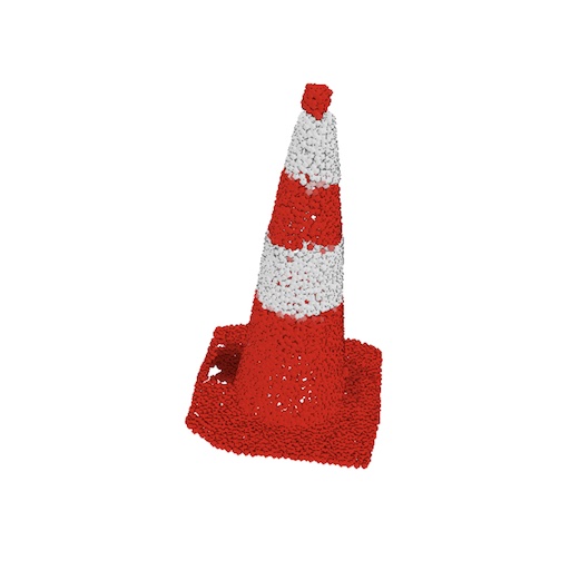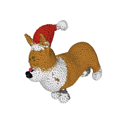
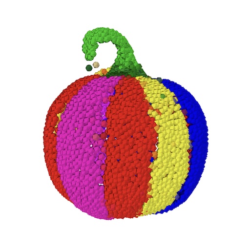
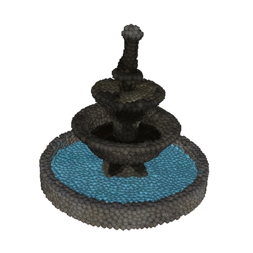
“a corgi wearing a red santa hat”	“a multicolored rainbow pumpkin”	“an elaborate fountain”	“a traffic cone”
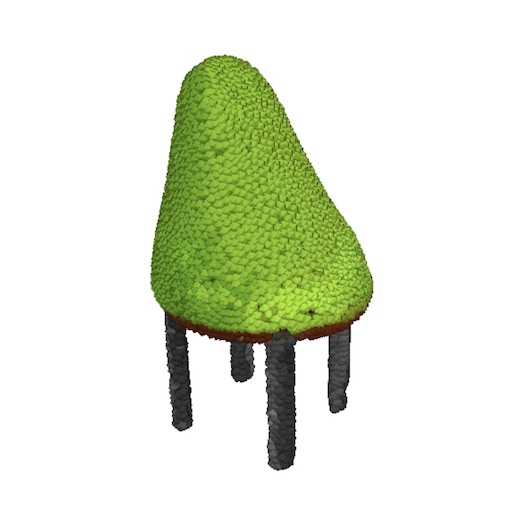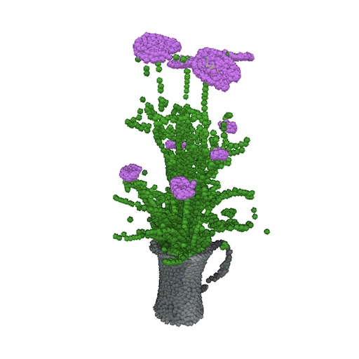
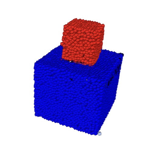
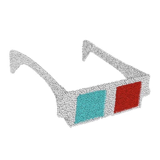
“a vase of purple flowers”	“a small red cube is sitting on top of a large blue cube. red on top, blue on bottom”	“a pair of 3d glasses, left lens is red right is blue”	“an avocado chair, a chair imitating an avocado”
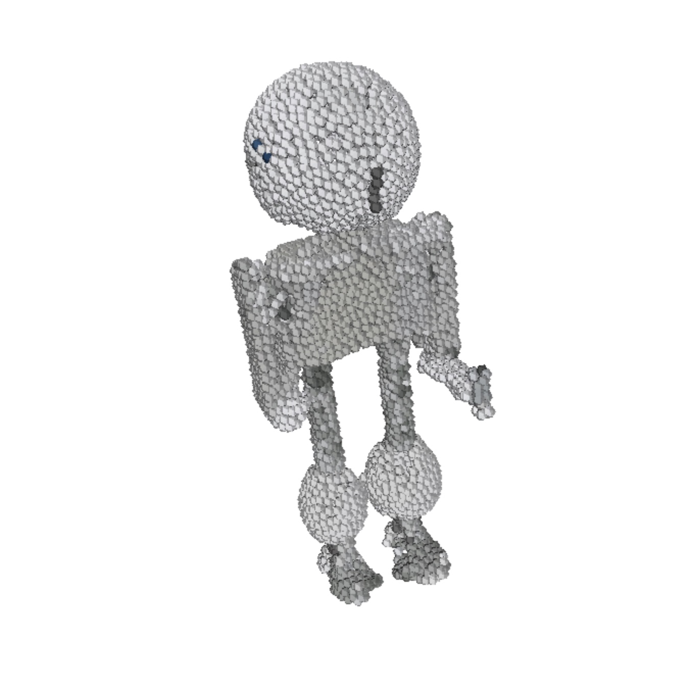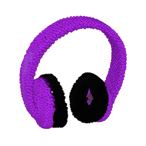
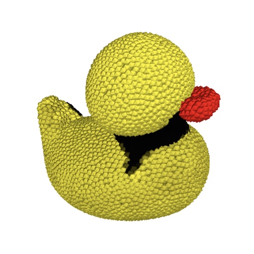
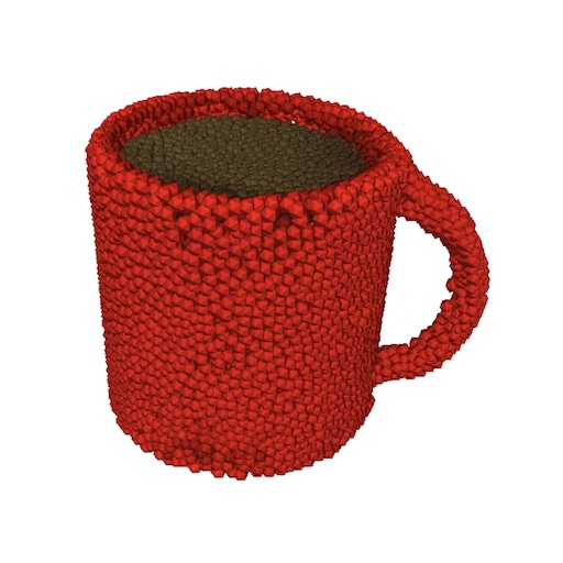
“a pair of purple headphones”	“a yellow rubber duck”	“a red mug filled with coffee”	“a humanoid robot with a round head”

Figure 2: Selected point clouds generated by Point$\cdot$E using the given text prompts. For each prompt, we selected one point cloud out of eight samples.

With the recent explosion of text-to-image generative models, it is now possible to generate and modify high-quality images from natural language descriptions in a number of seconds (Ramesh et al., 2021; Ding et al., 2021; Nichol et al., 2021; Ramesh et al., 2022; Gafni et al., 2022; Yu et al., 2022; Saharia et al., 2022; Feng et al., 2022; Balaji et al., 2022). Inspired by these results, recent works have explored text-conditional generation in other modalities, such as video (Hong et al., 2022; Singer et al., 2022; Ho et al., 2022b, a) and 3D objects (Jain et al., 2021; Poole et al., 2022; Lin et al., 2022a; Sanghi et al., 2021, 2022). In this work, we focus specifically on the problem of text-to-3D generation, which has significant potential to democratize 3D content creation for a wide range of applications such as virtual reality, gaming, and industrial design.

Recent methods for text-to-3D synthesis typically fall into one of two categories:

1. Methods which train generative models directly on paired (text, 3D) data (Chen et al., 2018; Mittal et al., 2022; Fu et al., 2022; Zeng et al., 2022) or unlabeled 3D data (Sanghi et al., 2021, 2022; Watson et al., 2022). While these methods can leverage existing generative modeling approaches to produce samples efficiently, they are difficult to scale to diverse and complex text prompts due to the lack of large-scale 3D datasets (Sanghi et al., 2022).

2. Methods which leverage pre-trained text-image models to optimize differentiable 3D representations (Jain et al., 2021; Poole et al., 2022; Lin et al., 2022a). These methods are often able to handle complex and diverse text prompts, but require expensive optimization processes to produce each sample. Furthermore, due to the lack of a strong 3D prior, these methods can fall into local minima which don’t correspond to meaningful or coherent 3D objects (Poole et al., 2022).

We aim to combine the benefits of both categories by pairing a text-to-image model with an image-to-3D model. Our text-to-image model leverages a large corpus of (text, image) pairs, allowing it to follow diverse and complex prompts, while our image-to-3D model is trained on a smaller dataset of (image, 3D) pairs. To produce a 3D object from a text prompt, we first sample an image using the text-to-image model, and then sample a 3D object conditioned on the sampled image. Both of these steps can be performed in a number of seconds, and do not require expensive optimization procedures. Figure 1 depicts this two-stage generation process.

We base our generative stack on diffusion (Sohl-Dickstein et al., 2015; Song & Ermon, 2020b; Ho et al., 2020), a recently proposed generative framework which has become a popular choice for text-conditional image generation. For our text-to-image model, we use a version of GLIDE (Nichol et al., 2021) fine-tuned on 3D renderings (Section 4.2). For our image-to-3D model, we use a stack of diffusion models which generate RGB point clouds conditioned on images (Section 4.3 and 4.4 detail our novel Transformer-based architecture for this task). For rendering-based evaluations, we go one step further and produce meshes from generated point clouds using a regression-based approach (Section 4.5).

We find that our system can often produce colored 3D point clouds that match both simple and complex text prompts (See Figure 2). We refer to our system as Point$\cdot$E, since it generates point clouds efficiently. We release our point cloud diffusion models, as well as evaluation code and models, at https://github.com/openai/point-e.

2 Background

Our method builds off of a growing body of work on diffusion-based models, which were first proposed by Sohl-Dickstein et al. (2015) and popularized more recently (Song & Ermon, 2020b, a; Ho et al., 2020).

We follow the Gaussian diffusion setup of Ho et al. (2020), which we briefly describe here. We aim to sample from some distribution $q(x_{0})$ using a neural network approximation $p_{\theta}(x_{0})$. Under Gaussian diffusion, we define a noising process

$$q(x_{t}|x_{t-1})\coloneqq\mathcal{N}(x_{t};\sqrt{1-\beta_{t}}x_{t-1},\beta_{t}\mathbf{I})$$

for integer timesteps $t\in[0,T]$. Intuitively, this process gradually adds Gaussian noise to a signal, with the amount of noise added at each timestep determined by some noise schedule $\beta_{t}$. We employ a noise schedule such that, by the final timestep $t=T$, the sample $x_{T}$ contains almost no information (i.e. it looks like Gaussian noise). Ho et al. (2020) note that it is possible to directly jump to a given timestep of the noising process without running the whole chain:

$$x_{t}=\sqrt{\bar{\alpha}_{t}}x_{0}+\sqrt{1-\bar{\alpha}_{t}}\epsilon$$

where $\epsilon\sim\mathcal{N}(0,\mathbf{I})$ and $\bar{\alpha}_{t}\coloneqq\prod_{s=0}^{t}1-\beta_{t}$.

To train a diffusion model, we approximate $q(x_{t-1}|x_{t})$ as a neural network $p_{\theta}(x_{t-1}|x_{t})$. We can then produce a sample by starting at random Gaussian noise $x_{T}$ and gradually reversing the noising process until arriving at a noiseless sample $x_{0}$. With enough small steps, $p_{\theta}(x_{t-1}|x_{t})$ can be parameterized as a diagonal Gaussian distribution, and Ho et al. (2020) propose to parameterize the mean of this distribution by predicting $\epsilon$, the effective noise added to a sample $x_{t}$. While Ho et al. (2020) fix the variance $\Sigma$ of $p_{\theta}(x_{t-1}|x_{t})$ to a reasonable per-timestep heuristic, Nichol & Dhariwal (2021) achieve better results by predicting the variance as well as the mean.

Diffusion sampling can be cast through the lens of differential equations (Song et al., 2020), allowing one to use various SDE and ODE solvers to sample from these models. Karras et al. (2022) find that a carefully-designed second-order ODE solver provides a good trade-off between quality and sampling efficiency, and we employ this sampler for our point cloud diffusion models.

To trade off sample diversity for fidelity in diffusion models, several guidance strategies may be used. Dhariwal & Nichol (2021) introduce classifier guidance, where gradients from a noise-aware classifier $\nabla_{x_{t}}p_{\theta}(y|x_{t})$ are used to perturb every sampling step. They find that increasing the scale of the perturbation increases generation fidelity while reducing sample diversity. Ho & Salimans (2021) introduce classifier-free guidance, wherein a conditional diffusion model $p(x_{t-1}|x_{t},y)$ is trained with the class label stochastically dropped and replaced with an additional $\varnothing$ class. During sampling, the model’s output $\epsilon$ is linearly extrapolated away from the unconditional prediction towards the conditional prediction:

$$\epsilon_{\textrm{guided}}\coloneqq\epsilon_{\theta}(x_{t},\varnothing)+s\cdot(\epsilon_{\theta}(x_{t},y)-\epsilon_{\theta}(x_{t},\varnothing))$$

for some guidance scale $s\geq 1$. This approach is straightforward to implement, requiring only that conditioning information is randomly dropped during training time. We employ this technique throughout our models, using the drop probability 0.1.

3 Related Work

Several prior works have explored generative models over point clouds. Achlioptas et al. (2017) train point cloud auto-encoders, and fit generative priors (either GANs (Goodfellow et al., 2014) or GMMs) on the resulting latent representations. Mo et al. (2019) generate point clouds using a VAE (Kingma & Welling, 2013) on hierarchical graph representations of 3D objects. Yang et al. (2019) train a two-stage flow model for point cloud generation: first, a prior flow model produces a latent vector, and then a second flow model samples points conditioned on the latent vector. Along the same lines, Luo & Hu (2021); Cai et al. (2020) both train two-stage models where the second stage is a diffusion model over individual points in a point cloud, and the first stage is a latent flow model or a latent GAN, respectively. Zeng et al. (2022) train a two-stage hierarchical VAE on point clouds with diffusion priors at both stages. Most similar to our work, Zhou et al. (2021a) introduce PVD, a single diffusion model that generates point clouds directly. Compared to previous point cloud diffusion methods such as PVD, our Transformer-based model architecture is simpler and incorporates less 3D-specific structure. Unlike prior works, our models also produce RGB channels alongside point cloud coordinates.

A growing body of work explores the problem of 3D model generation in representations other than point clouds. Several works aim to train 3D-aware GANs from datasets of 2D images (Chan et al., 2020; Schwarz et al., 2020; Chan et al., 2021; Or-El et al., 2021; Gu et al., 2021; Zhou et al., 2021b). These GANs are typically applied to the problem of novel view synthesis in forward-facing scenes, and do not attempt to reconstruct full 360-degree views of objects. More recently, Gao et al. (2022) train a GAN that directly produces full 3D meshes, paired with a discriminator that inputs differentiably-rendered (Laine et al., 2020) views of the generated meshes. Bautista et al. (2022) generates complete 3D scenes by first learning a representation space that decodes into NeRFs (Mildenhall et al., 2020), and then training a diffusion prior on this representation space. However, none of these works have demonstrated the ability to generate arbitrary 3D models conditioned on open-ended, complex text-prompts.

Several recent works have explored the problem of text-conditional 3D generation by optimizing 3D representations according to a text-image matching objective. Jain et al. (2021) introduce DreamFields, a method which optimizes the parameters of a NeRF using an objective based on CLIP (Radford et al., 2021). Notably, this method requires no 3D training data. Building on this principle, Khalid et al. (2022) optimizes a mesh using a CLIP-guided objective, finding that the mesh representation is more efficient to optimize than a NeRF. More recently, Poole et al. (2022) extend DreamFields to leverage a pre-trained text-to-image diffusion model instead of CLIP, producing more coherent and complex objects. Lin et al. (2022a) build off of this technique, but convert the NeRF representation into a mesh and then refine the mesh representation in a second optimization stage. While these approaches are able to produce diverse and complex objects or scenes, the optimization procedures typically require multiple GPU hours to converge, making them difficult to apply in practical settings.

While the above approaches are all based on optimization against a text-image model and do not leverage 3D data, other methods for text-conditional 3D synthesis make use of 3D data, possibly paired with text labels. Chen et al. (2018) employ a dataset of text-3D pairs to train a GAN to generate 3D representations conditioned on text. Liu et al. (2022) also leverage paired text-3D data to generate models in a joint representation space. Sanghi et al. (2021) employ a flow-based model to generate 3D latent representations, and find some text-to-3D capabilities when conditioning their model on CLIP embeddings. More recently, Zeng et al. (2022) achieve similar results when conditioning on CLIP embeddings, but employ a hierarchical VAE on point clouds for their generative stack. Mittal et al. (2022) and Fu et al. (2022) employ a VQ-VAE (van den Oord et al., 2017) with an autoregressive prior to sample 3D shapes conditioned on text labels. More recently, Sanghi et al. (2022) also employ a VQ-VAE approach, but leverage CLIP embeddings to avoid the need for explicit text labels in the dataset. While many of these works demonstrate promising early results, they tend to be limited to simple prompts or a narrow set of object categories due to the limited availability of 3D training data. Our method sidesteps this issue by leveraging a pre-trained text-to-image model to condition our 3D generation procedure.

A large body of research focuses on reconstructing 3D models from single or few images. Notably, this is an underspecified problem, since the model must impute some details not present in the conditioning image(s). Nevertheless, some regression-based methods have shown promising results on this task (Choy et al., 2016; Wang et al., 2018; Gkioxari et al., 2019; Groueix et al., 2018; Yu et al., 2020; Lin et al., 2022b). A separate body of literature studies generative approaches for single- or multi-view reconstruction. Fan et al. (2016) predict point clouds of objects from single views using a VAE. Sun et al. (2018) use a hybrid of a flow predictor and a GAN to generate novel views from few images. Kosiorek et al. (2021) use a view-conditional VAE to generate latent vectors for a NeRF decoder. Watson et al. (2022) employ an image-to-image diffusion model to synthesize novel views of an object conditioned on a single view, allowing many consistent views to be synthesized autoregressively.

4 Method

Rather than training a single generative model to directly produce point clouds conditioned on text, we instead break the generation process into three steps. First, we generate a synthetic view conditioned on a text caption. Next, we produce a coarse point cloud (1,024 points) conditioned on the synthetic view. And finally, we produce a fine point cloud (4,096 points) conditioned on the low-resolution point cloud and the synthetic view. In practice, we assume that the image contains the relevant information from the text, and do not explicitly condition the point clouds on the text.

To generate text-conditional synthetic views, we use a 3-billion parameter GLIDE model (Nichol et al., 2021) fine-tuned on rendered 3D models from our dataset (Section 4.2). To generate low-resolution point clouds, we use a conditional, permutation invariant diffusion model (Section 4.3). To upsample these low-resolution point clouds, we use a similar (but smaller) diffusion model which is additionally conditioned on the low-resolution point cloud (Section 4.4).

We train our models on a dataset of several million 3D models and associated metadata. We process the dataset into rendered views, text descriptions, and 3D point clouds with associated RGB colors for each point. We describe our data processing pipeline in more detail in Section 4.1.

4.1 Dataset

We train our models on several million 3D models. We found that data formats and quality varied wildly across our dataset, prompting us to develop various post-processing steps to ensure higher data quality.

To convert all of our data into one generic format, we rendered every 3D model from 20 random camera angles as RGBAD images using Blender (Community, 2018), which supports a variety of 3D formats and comes with an optimized rendering engine. For each model, our Blender script normalizes the model to a bounding cube, configures a standard lighting setup, and finally exports RGBAD images using Blender’s built-in realtime rendering engine.

We then converted each object into a colored point cloud using its renderings. In particular, we first constructed a dense point cloud for each object by computing points for each pixel in each RGBAD image. These point clouds typically contain hundreds of thousands of unevenly spaced points, so we additionally used farthest point sampling to create uniform clouds of 4K points. By constructing point clouds directly from renders, we were able to sidestep various issues that might arise from attempting to sample points directly from 3D meshes, such as sampling points which are contained within the model or dealing with 3D models that are stored in unusual file formats.

Finally, we employed various heuristics to reduce the frequency of low-quality models in our dataset. First, we eliminated flat objects by computing the SVD of each point cloud and only retaining those where the smallest singular value was above a certain threshold. Next, we clustered the dataset by CLIP features (for each object, we averaged features over all renders). We found that some clusters contained many low-quality categories of models, while other clusters appeared more diverse or interpretable. We binned these clusters into several buckets of varying quality, and used a weighted mixture of the resulting buckets as our final dataset.

4.2 View Synthesis GLIDE Model

Our point cloud models are conditioned on rendered views from our dataset, which were all produced using the same renderer and lighting settings. Therefore, to ensure that these models correctly handle generated synthetic views, we aim to explicitly generate 3D renders that match the distribution of our dataset.

To this end, we fine-tune GLIDE with a mixture of its original dataset and our dataset of 3D renderings. Since our 3D dataset is small compared to the original GLIDE training set, we only sample images from the 3D dataset 5% of the time, using the original dataset for the remaining 95%. We fine-tune for 100K iterations, meaning that the model has made several epochs over the 3D dataset (but has never seen the same exact rendered viewpoint twice).

To ensure that we always sample in-distribution renders (rather than only sampling them 5% of the time), we add a special token to every 3D render’s text prompt indicating that it is a 3D render; we then sample with this token at test time.

4.3 Point Cloud Diffusion

Figure 3: Our point cloud diffusion model architecture. Images are fed through a frozen, pre-trained CLIP model, and the output grid is fed as tokens into the transformer. Both the timestep $t$ and noised input $x_{t}$ are also fed in as tokens. The output tokens corresponding to $x_{t}$ are used to predict $\epsilon$ and $\Sigma$.

To generate point clouds with diffusion, we extend the framework used by Zhou et al. (2021a) to include RGB colors for each point in a point cloud. In particular, we represent a point cloud as a tensor of shape $K\times 6$, where $K$ is the number of points, and the inner dimension contains $(x,y,z)$ coordinates as well as $(R,G,B)$ colors. All coordinates and colors are normalized to the range $[-1,1]$. We then generate these tensors directly with diffusion, starting from random noise of shape $K\times 6$, and gradually denoising it.

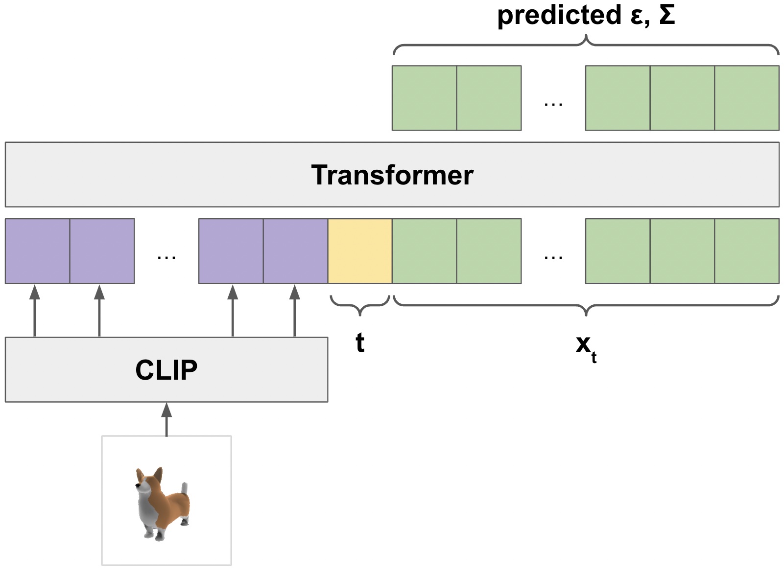
Unlike prior work which leverages 3D-specific architectures to process point clouds, we use a simple Transformer-based model (Vaswani et al., 2017) to predict both $\epsilon$ and $\Sigma$ conditioned on the image, timestep $t$, and noised point cloud $x_{t}$. An overview of our architecture can be seen in Figure 3. As input context to this model, we run each point in the point cloud through a linear layer with output dimension $D$, obtaining a $K\times D$ input tensor. Additionally, we run the timestep $t$ through a small MLP, obtaining another $D$-dimensional vector to prepend to the context.

To condition on the image, we feed it through a pre-trained ViT-L/14 CLIP model, take the last layer embeddings from this CLIP model (of shape $256\times D^{\prime}$), and linearly project it into another tensor of shape $256\times D$ before prepending it to the Transformer context. In Section 5.1, we find that this is superior to using a single CLIP image or text embedding, as done by Sanghi et al. (2021); Zeng et al. (2022); Sanghi et al. (2022).

The final input context to our model is of shape $(K+257)\times D$. To obtain a final output sequence of length $K$, we take the final $K$ tokens of output and project it to obtain $\epsilon$ and $\Sigma$ predictions for the $K$ input points.

Notably, we do not employ positional encodings for this model. As a result, the model itself is permutation-invariant to the input point clouds (although the output order is tied to the input order).

4.4 Point Cloud Upsampler

For image diffusion models, the best quality is typically achieved by using some form of hierarchy, where a low-resolution base model produces output which is then upsampled by another model (Nichol & Dhariwal, 2021; Saharia et al., 2021; Ho et al., 2021; Rombach et al., 2021). We employ this approach to point cloud generation by first generating 1K points with a large base model, and then upsampling to 4K points using a smaller upsampling model. Notably, our models’ compute requirements scale with the number of points, so it is four times more expensive to generate 4K points than 1K points for a fixed model size.

Our upsampler uses the same architecture as our base model, with extra conditioning tokens for the low-resolution point cloud. To arrive at 4K points, the upsampler conditions on 1K points and generates an additional 3K points which are added to the low-resolution pointcloud. We pass the conditioning points through a separate linear embedding layer than the one used for $x_{t}$, allowing the model to distinguish conditioning information from new points without requiring the use of positional embeddings.

4.5 Producing Meshes

For rendering-based evaluations, we do not render generated point clouds directly. Rather, we convert the point clouds into textured meshes and render these meshes using Blender. Producing meshes from point clouds is a well-studied, sometimes difficult problem. Point clouds produced by our models often have cracks, outliers, or other types of noise that make the problem particularly challenging. We briefly tried using pre-trained SAP models (Peng et al., 2021) for this purpose, but found that the resulting meshes sometimes lost large portions or important details of the shape that were present in the point clouds. Rather than training new SAP models, we opted to take a simpler approach.

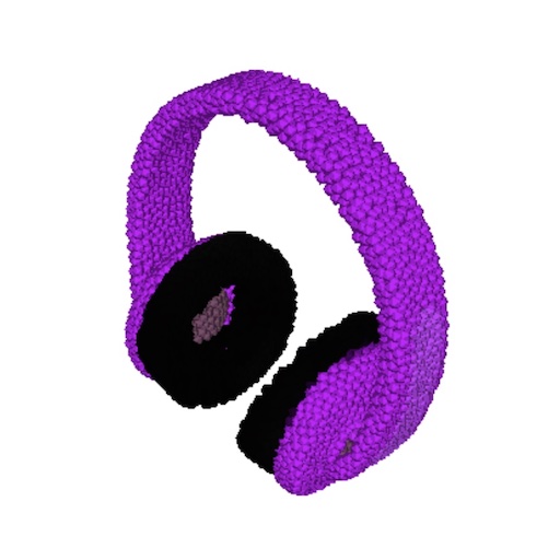
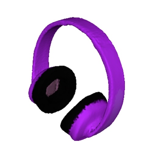
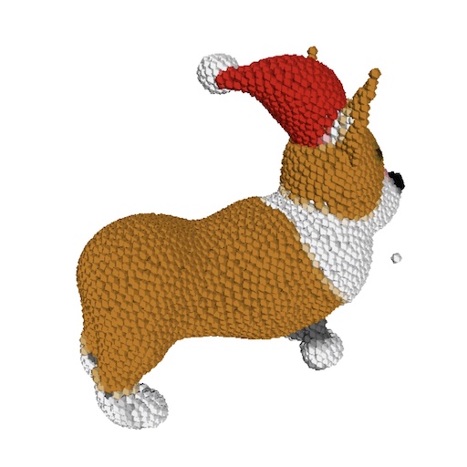
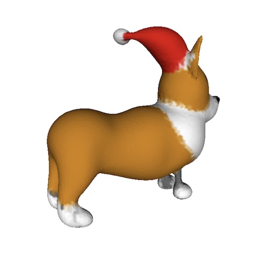
To convert point clouds into meshes, we use a regression-based model to predict the signed distance field of an object given its point cloud, and then apply marching cubes (Lorensen & Cline, 1987) to the resulting SDF to extract a mesh. We then assign colors to each vertex of the mesh using the color of the nearest point from the original point cloud. For details, see Appendix C.

5 Results

In the following sections, we conduct a number of ablations and comparisons to evaluate how our method performs and scales. We adopt the CLIP R-Precision (Park et al., 2021) metric for evaluating text-to-3D methods end-to-end, using the same object-centric evaluation prompts as Jain et al. (2021). Additionally, we introduce a new pair of metrics which we refer to as P-IS and P-FID, which are point cloud analogs for Inception Score (Salimans et al., 2016) and FID (Heusel et al., 2017), respectively.

To construct our P-IS and P-FID metrics, we employ a modified PointNet++ model (Qi et al., 2017) to extract features and predict class probabilities for point clouds. For details, see Appendix B.

5.1 Model Scaling and Ablations

(a) P-FID

(b) P-IS

(c) CLIP R-Precision

Figure 4: Sample-based evaluations computed throughout training across different base model runs. The same upsampler and conditioning images are used for all runs.

In this section, we train a variety of base diffusion models to study the effect of scaling and to ablate the importance of image conditioning. We train the following base models and evaluate them throughout training:

• 40M (uncond.): a small model without any conditioning information.

• 40M (text vec.): a small model which only conditions on text captions, not rendered images. The text caption is embedded with CLIP, and the CLIP embedding is appended as a single extra token of context. This model depends on the text captions present in our 3D dataset, and does not leverage the fine-tuned GLIDE model.

• 40M (image vec.): a small model which conditions on CLIP image embeddings of rendered images, similar to Sanghi et al. (2021). This differs from the other image-conditional models in that the image is encoded into a single token of context, rather than as a sequence of latents corresponding to the CLIP latent grid.

• 40M: a small model with full image conditioning through a grid of CLIP latents.

• 300M: a medium model with full image conditioning through a grid of CLIP latents.

• 1B: a large model with full image conditioning through a grid of CLIP latents.

In order to isolate changes to the base model, we use the same (image conditional) upsampler model for all evaluations, and use the same 306 pre-generated synthetic views for the CLIP R-Precision evaluation prompts. Here we use the ViT-L/14 CLIP model to compute CLIP R-Precision, but we report results with an alternative CLIP model in Section 5.3.

In Figure 4, we present the results of our ablations. We find that using only text conditioning with no text-to-image step results in much worse CLIP R-Precision (see Appendix E for more details). Furthermore, we find that using a single CLIP embedding to condition on images is worse than using a grid of embeddings, suggesting that the point cloud model benefits from seeing more (spatial) information about the conditioning image. Finally, we find that scaling our model improves the speed of P-FID convergence, and increases final CLIP R-Precision.

5.2 Qualitative Results

We find that Point$\cdot$E can often produce consistent and high-quality 3D shapes for complex prompts. In Figure 2, we show various point cloud samples which demonstrate our model’s ability to infer a variety of shapes while correctly binding colors to the relevant parts of the shapes.

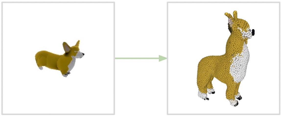
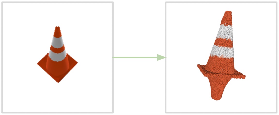
Sometimes the point cloud diffusion model fails to understand or extrapolate the conditioning image, resulting in a shape that does not match the original prompt. We find that this is usually due to one of two issues: 1) the model incorrectly interprets the shape of the object depicted in the image, or 2) the model incorrectly infers some part of the shape that is occluded in the image. In Figure 5, we present an example of each of these two failure modes.

(a) Image to point cloud sample for the prompt “a very realistic 3D rendering of a corgi”.

(b) Image to point cloud sample for the prompt “a traffic cone”.

Figure 5: Two common failure modes of our model. In the top example, the model incorrectly interprets the relative proportions of different parts of the depicted object, producing a tall dog instead of a short, long dog. In the bottom example, the model cannot see underneath the traffic cone, and incorrectly infers a second mirrored cone.

5.3 Comparison to Other Methods

Table 1: Comparison of Point$\cdot$E to other 3D generative techniques as measured by CLIP R-Precision (with two different CLIP base models) on COCO evaluation prompts. ^∗50 P100-minutes converted to V100-minutes using conversion rate $\frac{1}{3}$. ^†Assuming 2 V100 minutes = 1 A100 minute and 1 TPUv4-minute = 1 A100-minute. We report DreamFields results from Poole et al. (2022).

Method	ViT-B/32	ViT-L/14	Latency
DreamFields	78.6%	82.9%	$\sim 200$ V100-hr†
CLIP-Mesh	67.8%	74.5%	$\sim 17$ V100-min∗
DreamFusion	75.1%	79.7%	$\sim 12$ V100-hr†
Point$\cdot$E (40M, text-only)	15.4%	16.2%	16 V100-sec
Point$\cdot$E (40M)	36.5%	38.8%	1.0 V100-min
Point$\cdot$E (300M)	40.3%	45.6%	1.2 V100-min
Point$\cdot$E (1B)	41.1%	46.8%	1.5 V100-min
Conditioning images	69.6%	86.6%	-

As text-conditional 3D synthesis is a fairly new area of research, there is not yet a standard set of benchmarks for this task. However, several other works evaluate 3D generation using CLIP R-Precision, and we compare to these methods in Table 1. In addition to CLIP R-Precision, we also note the reported sampling compute requirements for each method.

While our method performs worse than the current state-of-the-art, we note two subtleties of this evaluation which may explain some (but likely not all) of this discrepancy:

• Unlike multi-view optimization-based methods like DreamFusion, Point$\cdot$E does not explicitly optimize every view to match the text prompt. This could result in lower CLIP R-Precision simply because certain objects are not easy to identify from all angles.

• Our method produces point clouds which must be preprocessed before rendering. Converting point clouds into meshes is a difficult problem, and the approach we use can sometimes lose information present in the point clouds themselves.

While our method performs worse on this evaluation than state-of-the-art techniques, it produces samples in a small fraction of the time. This could make it more practical for certain applications, or could allow for the discovery of higher-quality 3D objects by sampling many objects and selecting the best one according to some heuristic.

6 Limitations and Future Work

While our model is a meaningful step towards fast text-to-3D synthesis, it also has several limitations. Currently, our pipeline requires synthetic renderings, but this limitation could be lifted in the future by training 3D generators that condition on real-world images. Furthermore, while our method produces colored three-dimensional shapes, it does so at a relatively low resolution in a 3D format (point clouds) that does not capture fine-grained shape or texture. Extending this method to produce high-quality 3D representations such as meshes or NeRFs could allow the model’s outputs to be used for a variety of applications. Finally, our method could be used to initialize optimization-based techniques to speed up initial convergence.

We expect that this model shares many of the limitations, including bias, as our DALL$\cdot$E 2 system where many of the biases are inherited from the dataset (Mishkin et al., 2022). In addition, this model has the ability to support the creation of point clouds that can then be used to fabricate products in the real world, for example through 3D printing (Walther, 2014; Neely, 2016; Straub & Kerlin, 2016). This has implications both when the models are used to create blueprints for dangerous objects and when the blueprints are trusted to be safe despite no empirical validation (Figure 6).

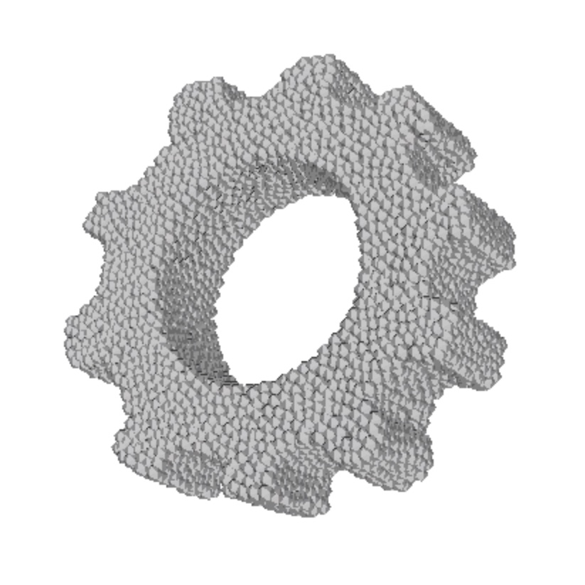“a 3D printable gear, a single gear 3 inches in diameter and half inch thick”

Figure 6: Example of a potential misuse of our model, where it could be used to fabricate objects in the real world without external validation.

7 Conclusion

We have presented Point$\cdot$E, a system for text-conditional synthesis of 3D point clouds that first generates synthetic views and then generates colored point clouds conditioned on these views. We find that Point$\cdot$E is capable of efficiently producing diverse and complex 3D shapes conditioned on text prompts. We hope that our approach can serve as a starting point for further work in the field of text-to-3D synthesis.

8 Acknowledgements

We would like to thank everyone behind ChatGPT for creating a tool that helped provide useful writing feedback.

Appendix A Hyperparameters

Table 2: Training hyper-parameters for our point cloud diffusion models. Width and depth refer to the size of the transformer backbone.

Model	Width	Depth	LR	# Params
Base (40M)	512	12	1e-4	40,466,956
Base (300M)	1024	24	7e-5	311,778,316
Base (1B)	2048	24	5e-5	1,244,311,564
Upsampler	512	12	1e-4	40,470,540

We train all of our diffusion models with batch size 64 for 1,300,000 iterations. In Table 2, we enumerate the training hyperparameters that were varied across model sizes. We train all of our models with 1024 diffusion timesteps. For our upsampler model, we use the linear noise schedule from Ho et al. (2020), and for our base models, we use the cosine noise schedule proposed by Nichol & Dhariwal (2021).

Table 3: Sampling hyperparameters for figures and CLIP R-Precision evaluations.

Hyperparameter	Base	Upsampler
Timesteps	64	64
Guidance scale	3.0	3.0
$S_{\text{churn}}$	3	0
$\sigma_{\text{min}}$	1e-3	1e-3
$\sigma_{\text{max}}$	120	160

For P-FID and P-IS evaluations, we produce 10K samples using stochastic DDPM with the full noise schedule. For CLIP R-Precision and figures in the paper, we use 64 steps (128 function evaluations) of the Heun sampler from Karras et al. (2022) for both the base and upsampler models. Table 3 enumerates the hyperparameters used for Heun sampling. When sampling from GLIDE, we use 150 diffusion steps for the base model, and 50 diffusion steps for the upsampling model. We report sampling time for each component of our stack in Table 4.

Table 4: Sampling performance for various components of our model. We use the Karras sampler for our base and upsampler models, but not for GLIDE.

Model	V100 seconds
GLIDE	46.28
Upsampler (40M)	12.58
Base (40M)	3.35
Base (300M)	12.78
Base (1B)	28.67

Appendix B P-FID and P-IS Metrics

To evaluate P-FID and P-IS, we train a PointNet++ model on ModelNet40 (Wu et al., 2015) using an open source implementation. We modify the baseline model in several ways. First, we double the width of the model, resulting in roughly 16 million parameters. Next, we apply some additional data augmentations to make the model more robust to out-of-distribution samples. In particular, we apply random rotations to each point cloud, and we add Gaussian noise to the points with standard deviation sampled from $U[0,0.01]$.

To compute P-FID, we extract features for each point cloud from the layer before the final ReLU activation. To compute P-IS, we use the predicted class probabilities for the 40 classes from ModelNet40. We note that our generative models are trained on a dataset which only has P-IS 12.95, so our best reported P-IS score of $\sim 13$ is near the expected upper bound.

Appendix C Mesh Extraction

To convert point clouds into meshes, we train a model which predicts SDFs from point clouds and apply marching cubes to the resulting SDFs. We parametrize our SDF model as an encoder-decoder Transformer. First, an 8-layer encoder processes the input point cloud as an unordered sequence, producing a sequence of hidden representations. Then, a 4-layer cross-attention decoder takes 3D coordinates and the sequence of latent vectors, and predicts an SDF value. Each input query point is processed independently, allowing for efficient batching. Using more layers in the encoder and fewer in the decoder allows us to amortize the encoding cost across many query points.

We train our SDF regression model on a subset of 2.4 million manifold meshes from our dataset, and add Gaussian noise with $\sigma=0.005$ to the point clouds as data augmentation. We train the model $f_{\theta}(x)$ to predict the SDF $y$ with a weighted L1 objective:

$$\begin{cases}1\cdot||f_{\theta}(x)-y||_{1}&f_{\theta}(x)>y\\ 4\cdot||f_{\theta}(x)-y||_{1}&f_{\theta}(x)\leq y\end{cases}$$

Here, we define the SDF such that points outside of the surface have negative sign. Therefore, in the face of uncertainty, the model is encouraged predict that points are inside the surface. We found this to be helpful in initial experiments, likely because it helps prevent the resulting meshes from effectively ignoring thin or noisy parts of the point cloud.

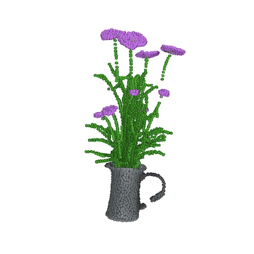
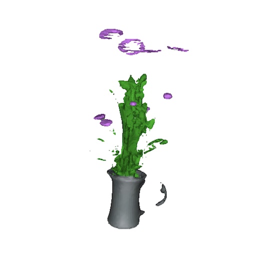
When producing meshes for evaluations, we use a grid size of $128\times 128\times 128$, resulting in $128^{3}$ queries to the SDF model. In Figure 7, we show examples of input point clouds and corresponding output meshes from our model. We observe that our method works well in many cases, but sometimes fails to capture thin or sparse parts of a point cloud.

Figure 7: Examples of point clouds (left) and corresponding extracted meshes (right). We find that our method often produces smooth meshes and removes outliers (middle row), but can sometimes miss thin/sparse parts of objects (bottom row).

Appendix D Conditioning on DALL$\cdot$E 2 Samples

Figure 8: Examples of point clouds reconstructed from DALL$\cdot$2 generations. The top image was produced using the prompt “a 3d rendering of an avocado chair, chair imitating an avocado, full view, white background”. The middle image was produced using the prompt “a simple full view of a 3d rendering of a corgi in front of a white background”. The bottom image is the same as the middle image, but with an additional white border.

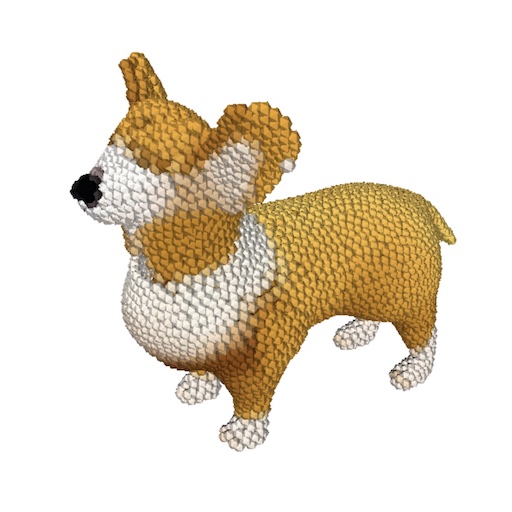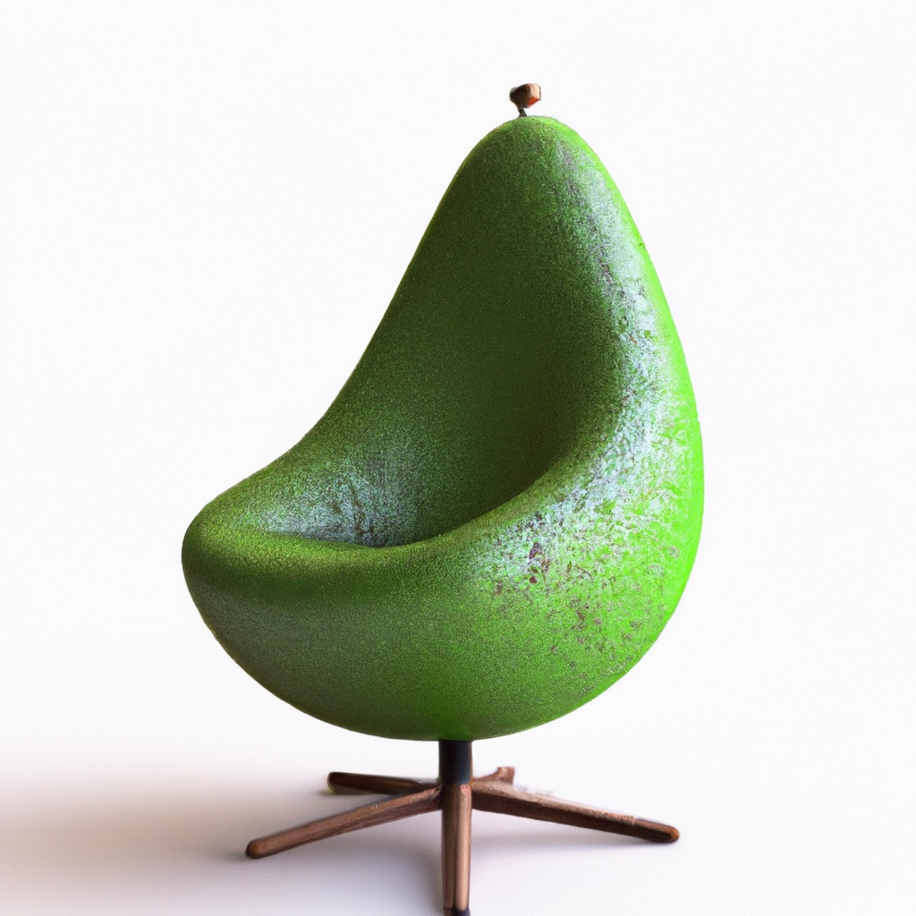
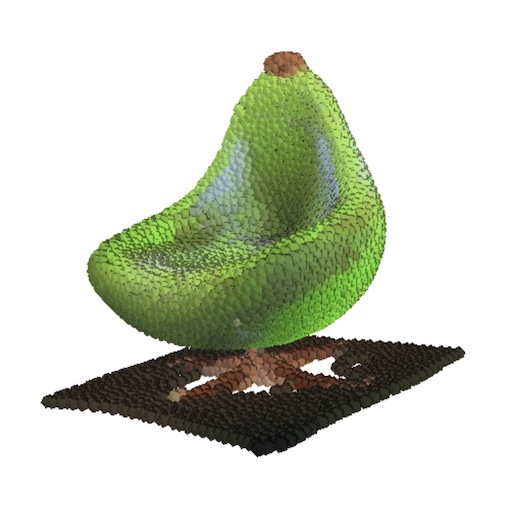
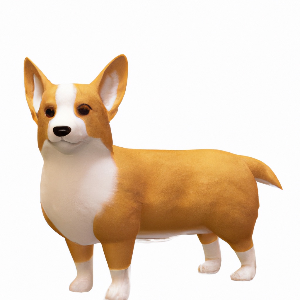
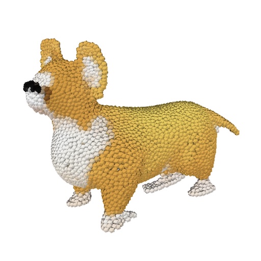
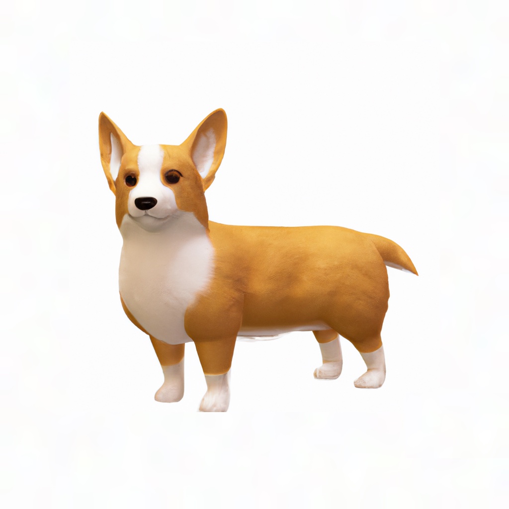
In our main experiments, we use a specialized text-to-image model to produce in-distribution conditioning images for our point cloud models. In this section, we explore what happens if we use renders from a pre-existing text-to-image model, DALL$\cdot$E 2.

In Figure 8, we present three image-to-3D examples where the conditioning images are generated by DALL$\cdot$E 2. We find that DALL$\cdot$E 2 tends to include shadows under objects, and our point cloud model interprets these as a dark ground plane. We also find that our point cloud model can misinterpret shapes from the generated images when the objects take up too much of the image. In these cases, adding a border around the generated images can improve the reconstructed shapes.

Appendix E Pure Text-Conditional Generation

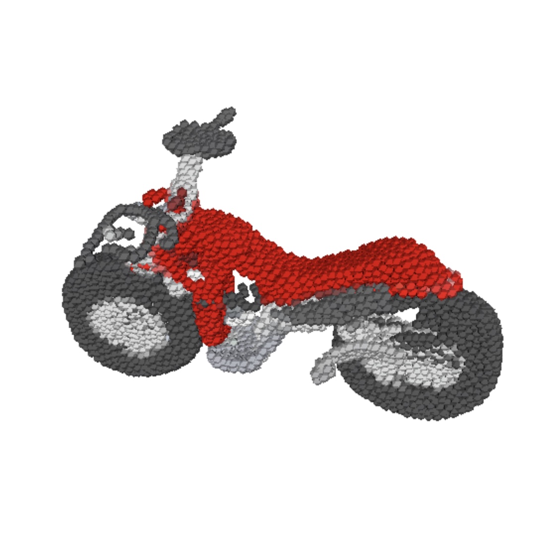
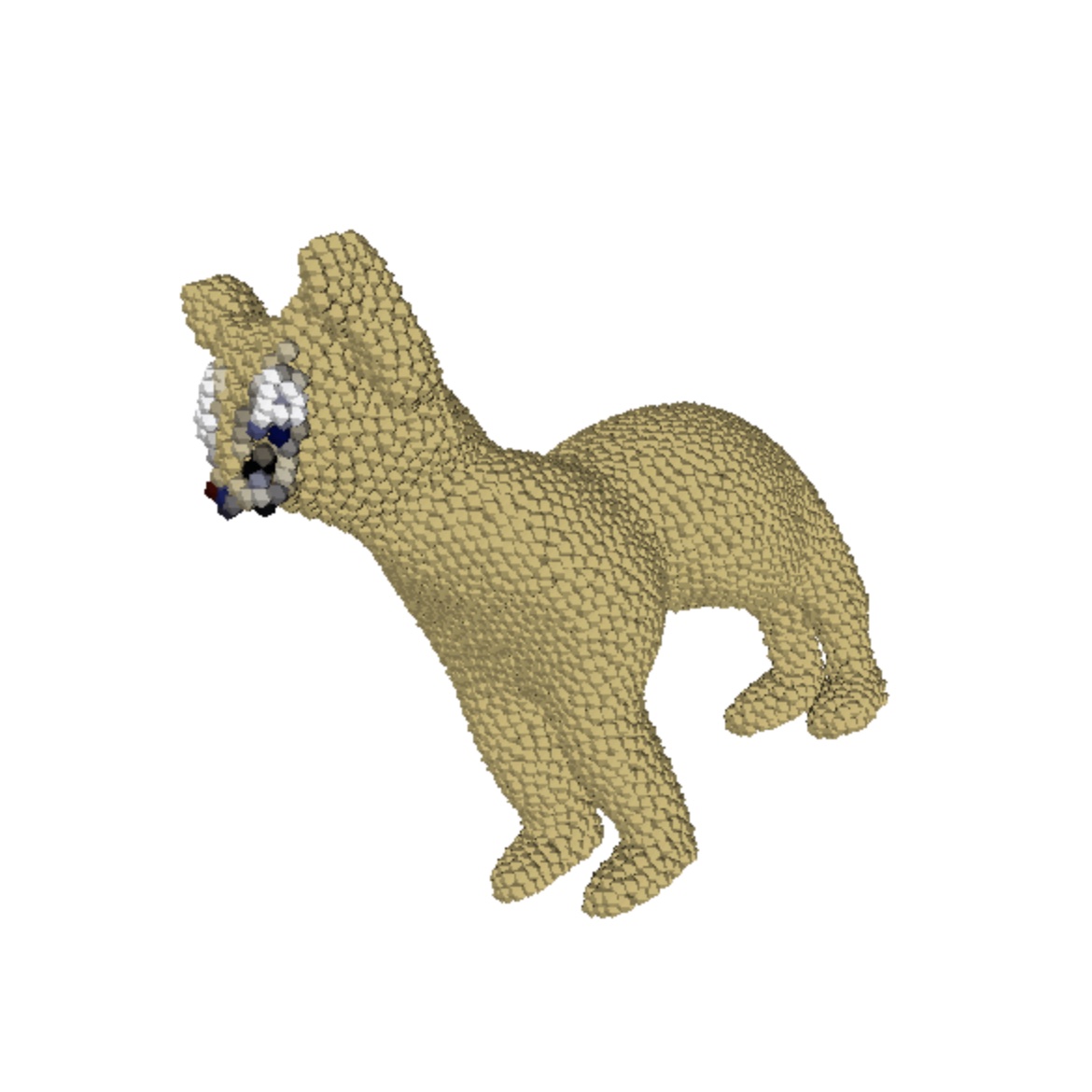
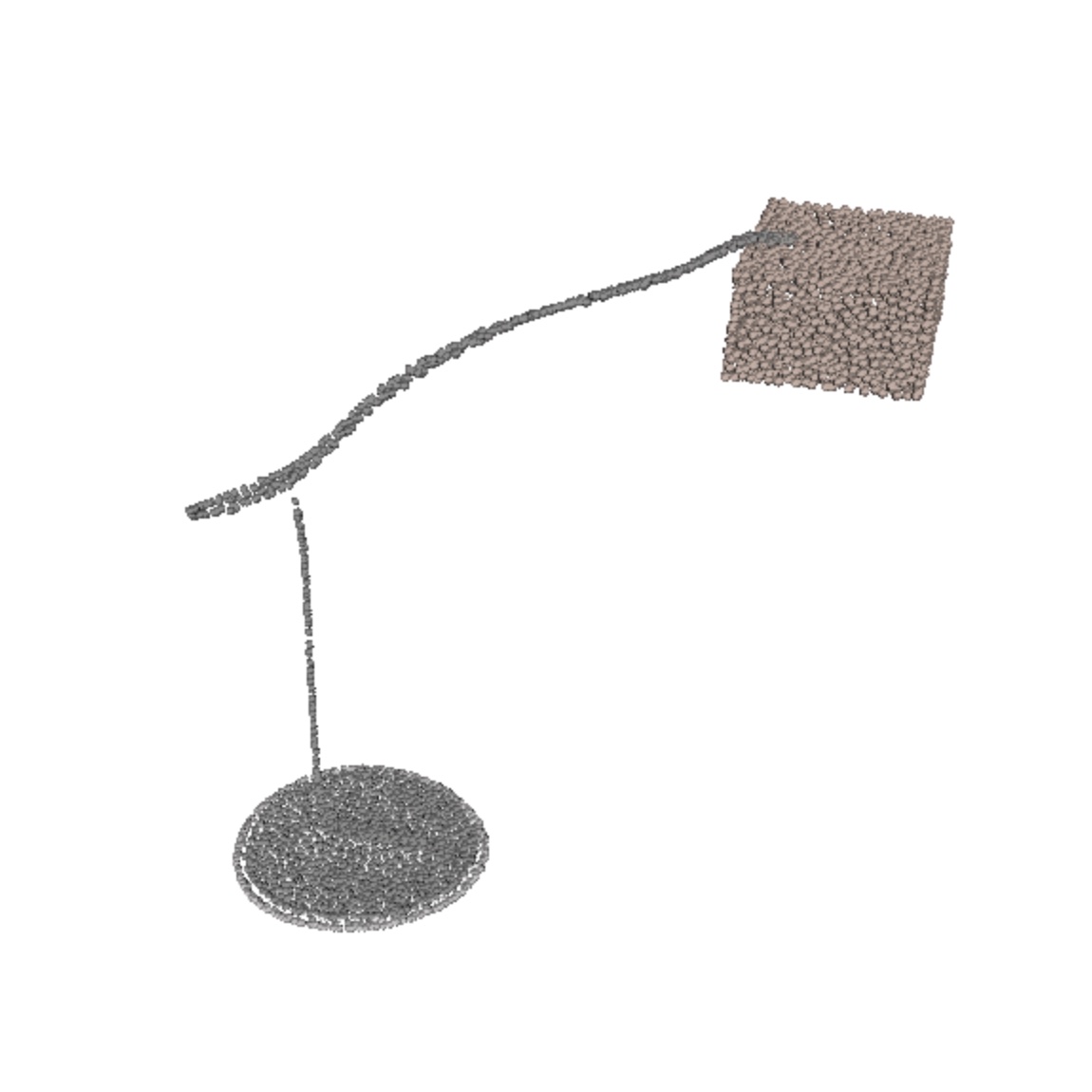
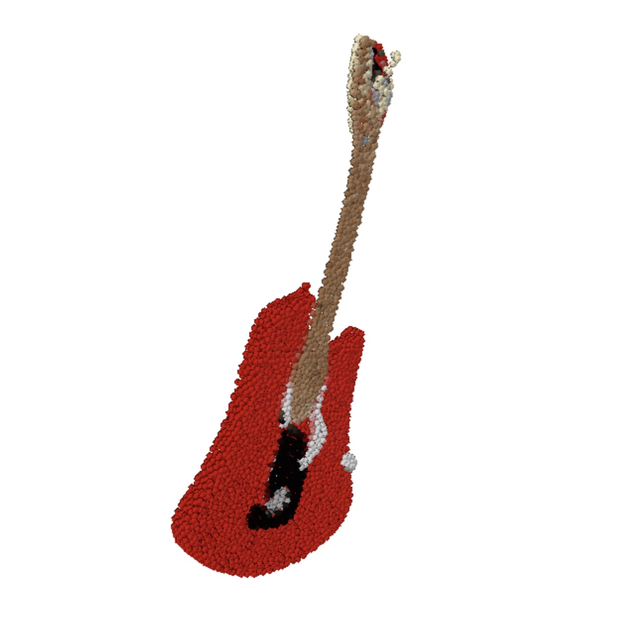
In Section 5.1, we train a pure text-conditional point cloud model without an additional image generation step. While we find that this model performs worse on evaluations than our full system, it still achieves non-trivial results. In this section, we explore the capabilities and limitations of this model.

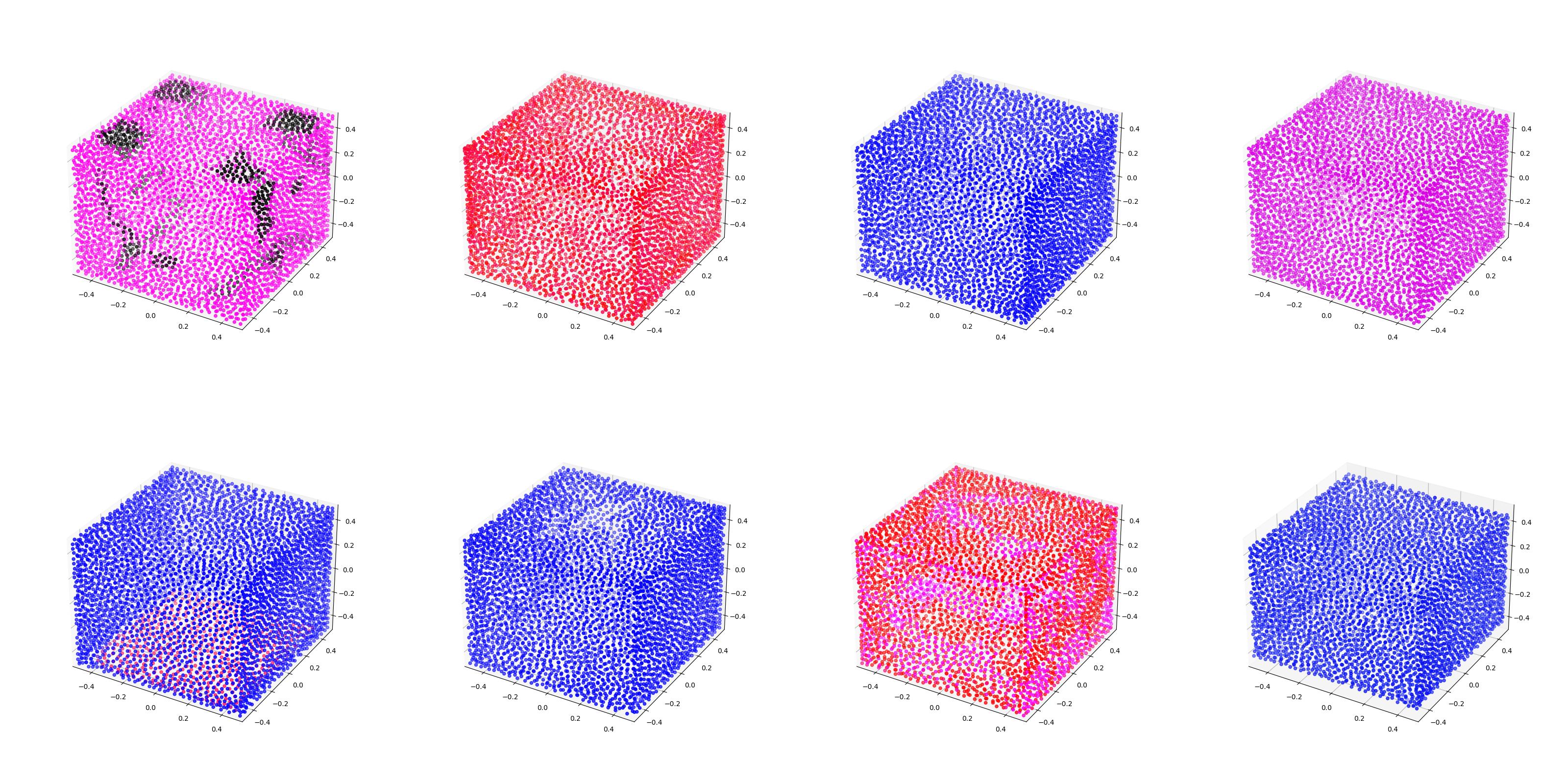
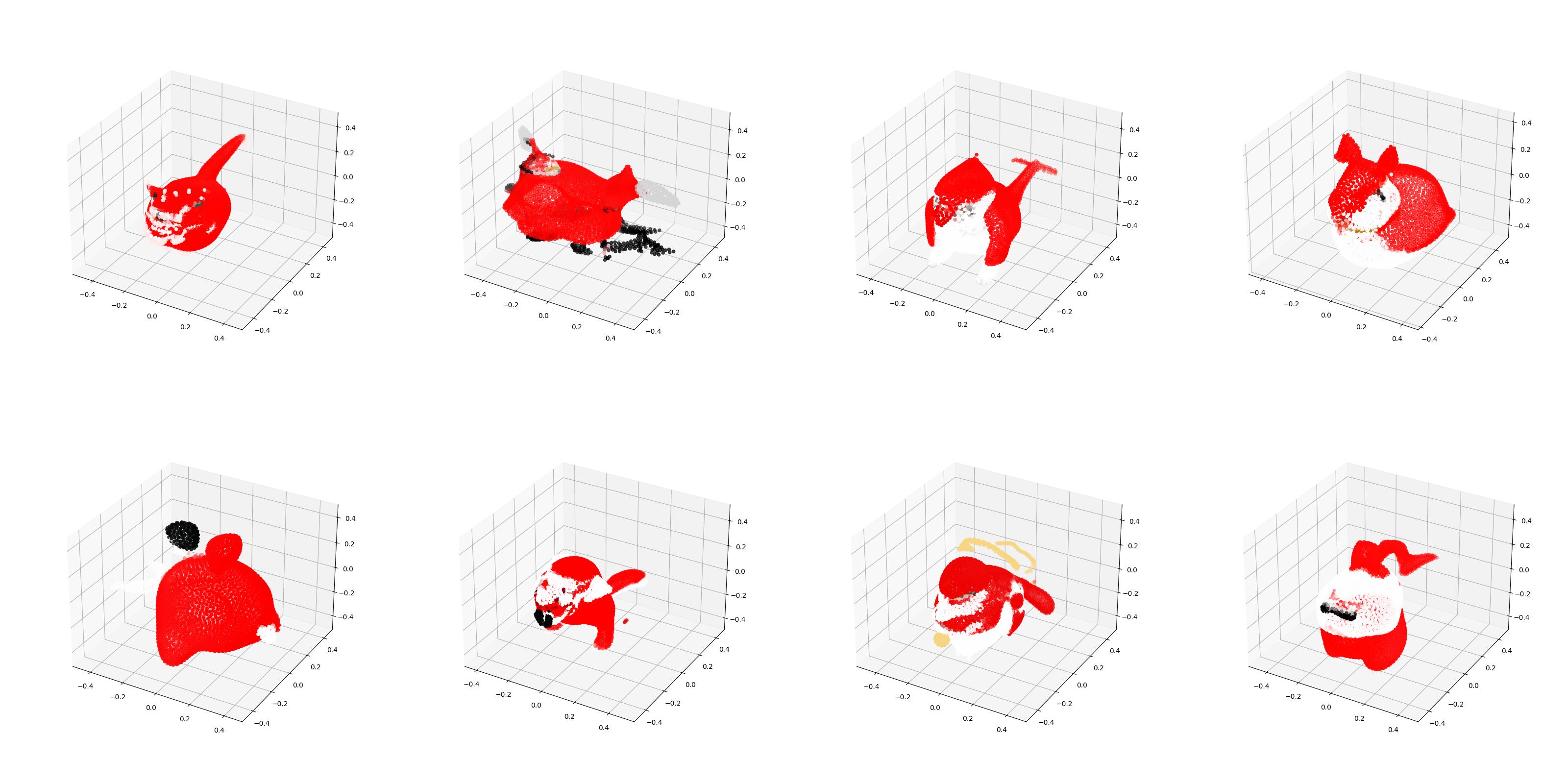
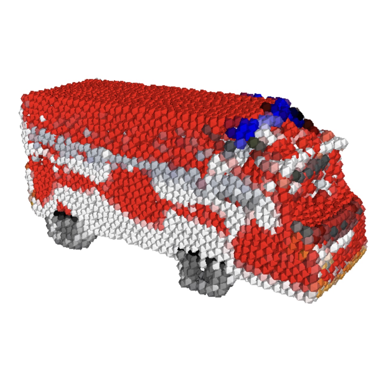
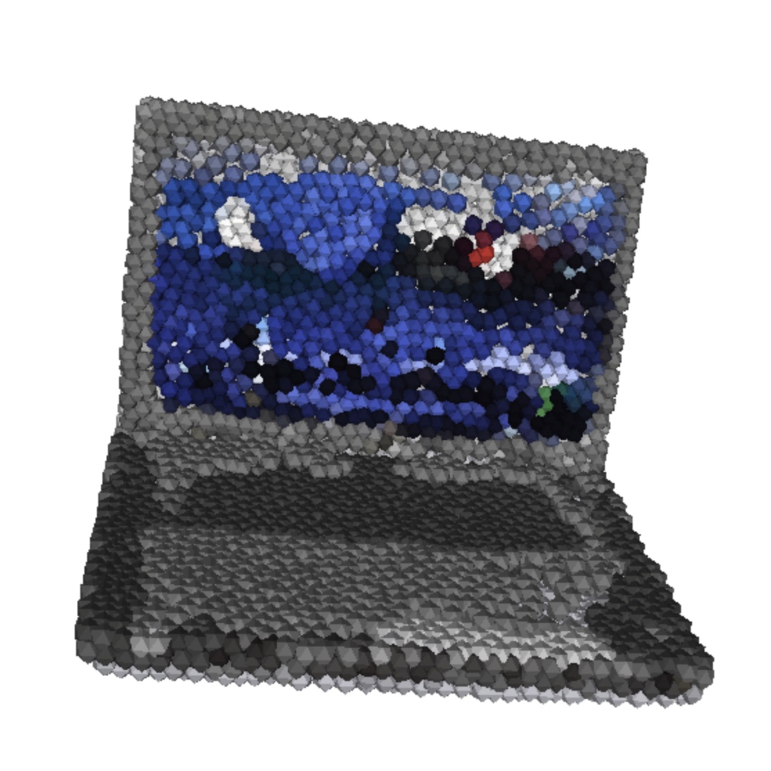
In Figure 9, we show examples where our text-conditional model is able to produce point clouds matching the provided text prompt. Notably, these examples include simple prompts that describe single objects. In Figure 10, we show examples where this model struggles with prompts that combine multiple concepts.

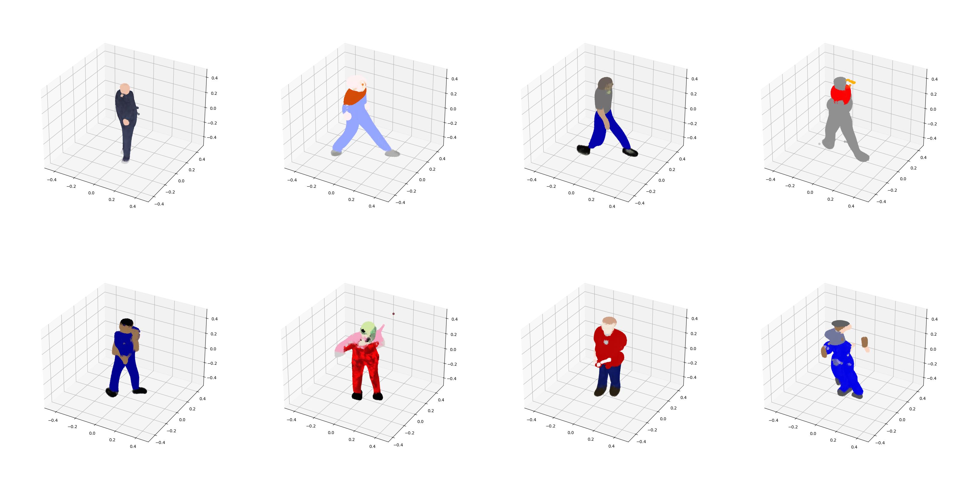
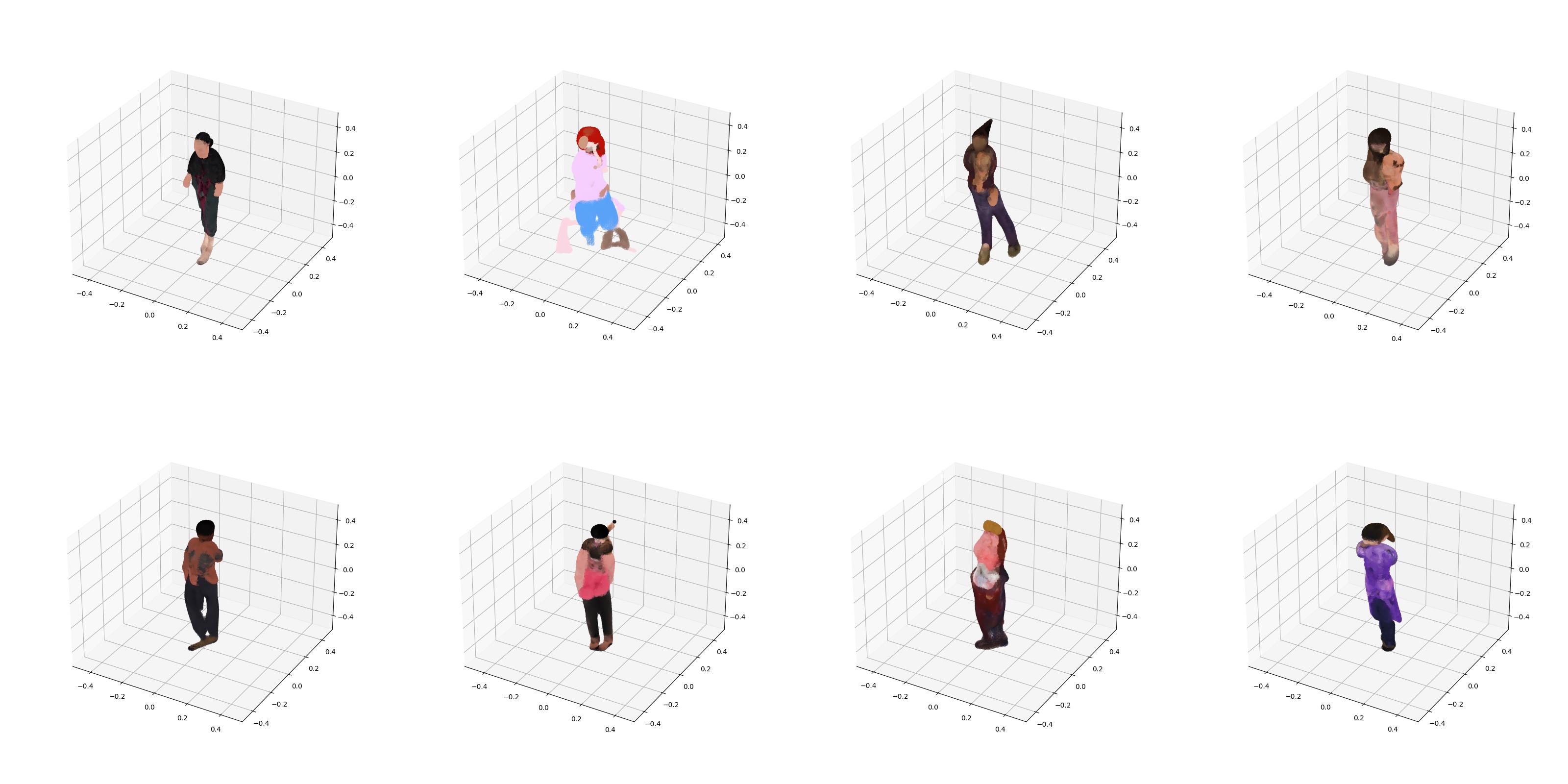
Finally, we expect that this model has inherited biases from our 3D dataset. We present one possible example of this in Figure 11, wherein the model produces longer and narrower objects for the prompt “a woman” than for the prompt “a man” when using a fixed diffusion noise seed.

“a motorbike”	“a dog”
“a desk lamp”	“a guitar”
“an ambulance”	“a laptop computer”

Figure 9: Selected point clouds generated by our pure text-conditional 40M parameter point cloud diffusion model.

(a) Prompt: “a small red cube is sitting on top of a large blue cube. red on top, blue on bottom”

(b) Prompt: “a corgi wearing a red santa hat”

Figure 10: Sample grids where our small, pure text-conditional model fails to understand complex prompts.

(a) Prompt: “a man”

(b) Prompt: “a woman”

Figure 11: Sample grids from our pure text-conditional 40M parameter model. Samples in the top grid use the same noise seed as the corresponding samples in the bottom grid.

References

- Achlioptas et al. (2017) Achlioptas, P., Diamanti, O., Mitliagkas, I., and Guibas, L. Learning representations and generative models for 3d point clouds. arXiv:1707.02392, 2017.
- Balaji et al. (2022) Balaji, Y., Nah, S., Huang, X., Vahdat, A., Song, J., Kreis, K., Aittala, M., Aila, T., Laine, S., Catanzaro, B., Karras, T., and Liu, M.-Y. ediff-i: Text-to-image diffusion models with an ensemble of expert denoisers, 2022.
- Bautista et al. (2022) Bautista, M. A., Guo, P., Abnar, S., Talbott, W., Toshev, A., Chen, Z., Dinh, L., Zhai, S., Goh, H., Ulbricht, D., Dehghan, A., and Susskind, J. Gaudi: A neural architect for immersive 3d scene generation. arXiv:2207.13751, 2022.
- Cai et al. (2020) Cai, R., Yang, G., Averbuch-Elor, H., Hao, Z., Belongie, S., Snavely, N., and Hariharan, B. Learning gradient fields for shape generation. arXiv:2008.06520, 2020.
- Chan et al. (2020) Chan, E. R., Monteiro, M., Kellnhofer, P., Wu, J., and Wetzstein, G. pi-gan: Periodic implicit generative adversarial networks for 3d-aware image synthesis. arXiv:2012.00926, 2020.
- Chan et al. (2021) Chan, E. R., Lin, C. Z., Chan, M. A., Nagano, K., Pan, B., Mello, S. D., Gallo, O., Guibas, L., Tremblay, J., Khamis, S., Karras, T., and Wetzstein, G. Efficient geometry-aware 3d generative adversarial networks. arXiv:2112.07945, 2021.
- Chen et al. (2018) Chen, K., Choy, C. B., Savva, M., Chang, A. X., Funkhouser, T., and Savarese, S. Text2shape: Generating shapes from natural language by learning joint embeddings. arXiv:1803.08495, 2018.
- Choy et al. (2016) Choy, C. B., Xu, D., Gwak, J., Chen, K., and Savarese, S. 3d-r2n2: A unified approach for single and multi-view 3d object reconstruction. arXiv:1604.00449, 2016.
- Community (2018) Community, B. O. Blender - a 3D modelling and rendering package. Blender Foundation, Stichting Blender Foundation, Amsterdam, 2018. URL http://www.blender.org.
- Dhariwal & Nichol (2021) Dhariwal, P. and Nichol, A. Diffusion models beat gans on image synthesis. arXiv:2105.05233, 2021.
- Ding et al. (2021) Ding, M., Yang, Z., Hong, W., Zheng, W., Zhou, C., Yin, D., Lin, J., Zou, X., Shao, Z., Yang, H., and Tang, J. Cogview: Mastering text-to-image generation via transformers. arXiv:2105.13290, 2021.
- Fan et al. (2016) Fan, H., Su, H., and Guibas, L. A point set generation network for 3d object reconstruction from a single image. arXiv:1612.00603, 2016.
- Feng et al. (2022) Feng, Z., Zhang, Z., Yu, X., Fang, Y., Li, L., Chen, X., Lu, Y., Liu, J., Yin, W., Feng, S., Sun, Y., Tian, H., Wu, H., and Wang, H. Ernie-vilg 2.0: Improving text-to-image diffusion model with knowledge-enhanced mixture-of-denoising-experts. arXiv:2210.15257, 2022.
- Fu et al. (2022) Fu, R., Zhan, X., Chen, Y., Ritchie, D., and Sridhar, S. Shapecrafter: A recursive text-conditioned 3d shape generation model. arXiv:2207.09446, 2022.
- Gafni et al. (2022) Gafni, O., Polyak, A., Ashual, O., Sheynin, S., Parikh, D., and Taigman, Y. Make-a-scene: Scene-based text-to-image generation with human priors. arXiv:2203.13131, 2022.
- Gao et al. (2022) Gao, J., Shen, T., Wang, Z., Chen, W., Yin, K., Li, D., Litany, O., Gojcic, Z., and Fidler, S. Get3d: A generative model of high quality 3d textured shapes learned from images. arXiv:2209.11163, 2022.
- Gkioxari et al. (2019) Gkioxari, G., Malik, J., and Johnson, J. Mesh r-cnn. arXiv:1906.02739, 2019.
- Goodfellow et al. (2014) Goodfellow, I. J., Pouget-Abadie, J., Mirza, M., Xu, B., Warde-Farley, D., Ozair, S., Courville, A., and Bengio, Y. Generative adversarial networks. arXiv:1406.2661, 2014.
- Groueix et al. (2018) Groueix, T., Fisher, M., Kim, V. G., Russell, B. C., and Aubry, M. Atlasnet: A papier-mâché approach to learning 3d surface generation. arXiv:1802.05384, 2018.
- Gu et al. (2021) Gu, J., Liu, L., Wang, P., and Theobalt, C. Stylenerf: A style-based 3d-aware generator for high-resolution image synthesis. arXiv:2110.08985, 2021.
- Heusel et al. (2017) Heusel, M., Ramsauer, H., Unterthiner, T., Nessler, B., and Hochreiter, S. Gans trained by a two time-scale update rule converge to a local nash equilibrium. Advances in Neural Information Processing Systems 30 (NIPS 2017), 2017.
- Ho & Salimans (2021) Ho, J. and Salimans, T. Classifier-free diffusion guidance. In NeurIPS 2021 Workshop on Deep Generative Models and Downstream Applications, 2021. URL https://openreview.net/forum?id=qw8AKxfYbI.
- Ho et al. (2020) Ho, J., Jain, A., and Abbeel, P. Denoising diffusion probabilistic models. arXiv:2006.11239, 2020.
- Ho et al. (2021) Ho, J., Saharia, C., Chan, W., Fleet, D. J., Norouzi, M., and Salimans, T. Cascaded diffusion models for high fidelity image generation. arXiv:2106.15282, 2021.
- Ho et al. (2022a) Ho, J., Chan, W., Saharia, C., Whang, J., Gao, R., Gritsenko, A., Kingma, D. P., Poole, B., Norouzi, M., Fleet, D. J., and Salimans, T. Imagen video: High definition video generation with diffusion models. arXiv:2210.02303, 2022a.
- Ho et al. (2022b) Ho, J., Salimans, T., Gritsenko, A., Chan, W., Norouzi, M., and Fleet, D. J. Video diffusion models. arXiv:2204.03458, 2022b.
- Hong et al. (2022) Hong, W., Ding, M., Zheng, W., Liu, X., and Tang, J. Cogvideo: Large-scale pretraining for text-to-video generation via transformers. arXiv:2205.15868, 2022.
- Jain et al. (2021) Jain, A., Mildenhall, B., Barron, J. T., Abbeel, P., and Poole, B. Zero-shot text-guided object generation with dream fields. arXiv:2112.01455, 2021.
- Karras et al. (2022) Karras, T., Aittala, M., Aila, T., and Laine, S. Elucidating the design space of diffusion-based generative models. arXiv:2206.00364, 2022.
- Khalid et al. (2022) Khalid, N. M., Xie, T., Belilovsky, E., and Popa, T. Clip-mesh: Generating textured meshes from text using pretrained image-text models. arXiv:2203.13333, 2022.
- Kingma & Welling (2013) Kingma, D. P. and Welling, M. Auto-encoding variational bayes. arXiv:1312.6114, 2013.
- Kosiorek et al. (2021) Kosiorek, A. R., Strathmann, H., Zoran, D., Moreno, P., Schneider, R., Mokrá, S., and Rezende, D. J. NeRF-VAE: A geometry aware 3D scene generative model. arXiv:2104.00587, April 2021.
- Laine et al. (2020) Laine, S., Hellsten, J., Karras, T., Seol, Y., Lehtinen, J., and Aila, T. Modular primitives for high-performance differentiable rendering. arXiv:2011.03277, 2020.
- Lin et al. (2022a) Lin, C.-H., Gao, J., Tang, L., Takikawa, T., Zeng, X., Huang, X., Kreis, K., Fidler, S., Liu, M.-Y., and Lin, T.-Y. Magic3d: High-resolution text-to-3d content creation. arXiv:2211.10440, 2022a.
- Lin et al. (2022b) Lin, K.-E., Yen-Chen, L., Lai, W.-S., Lin, T.-Y., Shih, Y.-C., and Ramamoorthi, R. Vision transformer for nerf-based view synthesis from a single input image. arXiv:2207.05736, 2022b.
- Liu et al. (2022) Liu, Z., Wang, Y., Qi, X., and Fu, C.-W. Towards implicit text-guided 3d shape generation. arXiv:2203.14622, 2022.
- Lorensen & Cline (1987) Lorensen, W. E. and Cline, H. E. Marching cubes: A high resolution 3d surface construction algorithm. In Stone, M. C. (ed.), SIGGRAPH, pp. 163–169. ACM, 1987. ISBN 0-89791-227-6. URL http://dblp.uni-trier.de/db/conf/siggraph/siggraph1987.html#LorensenC87.
- Luo & Hu (2021) Luo, S. and Hu, W. Diffusion probabilistic models for 3d point cloud generation. arXiv:2103.01458, 2021.
- Mildenhall et al. (2020) Mildenhall, B., Srinivasan, P. P., Tancik, M., Barron, J. T., Ramamoorthi, R., and Ng, R. Nerf: Representing scenes as neural radiance fields for view synthesis. arXiv:2003.08934, 2020.
- Mishkin et al. (2022) Mishkin, P., Ahmad, L., Brundage, M., Krueger, G., and Sastry, G. Dall·e 2 preview - risks and limitations. 2022. URL https://github.com/openai/dalle-2-preview/blob/main/system-card.md.
- Mittal et al. (2022) Mittal, P., Cheng, Y.-C., Singh, M., and Tulsiani, S. Autosdf: Shape priors for 3d completion, reconstruction and generation. arXiv:2203.09516, 2022.
- Mo et al. (2019) Mo, K., Guerrero, P., Yi, L., Su, H., Wonka, P., Mitra, N., and Guibas, L. J. Structurenet: Hierarchical graph networks for 3d shape generation. arXiv:1908.00575, 2019.
- Neely (2016) Neely, E. L. The risks of revolution: Ethical dilemmas in 3d printing from a us perspective. Science and Engineering Ethics, 22(5):1285–1297, Oct 2016. ISSN 1471-5546. doi: 10.1007/s11948-015-9707-4. URL https://doi.org/10.1007/s11948-015-9707-4.
- Nichol & Dhariwal (2021) Nichol, A. and Dhariwal, P. Improved denoising diffusion probabilistic models. arXiv:2102.09672, 2021.
- Nichol et al. (2021) Nichol, A., Dhariwal, P., Ramesh, A., Shyam, P., Mishkin, P., McGrew, B., Sutskever, I., and Chen, M. Glide: Towards photorealistic image generation and editing with text-guided diffusion models. arXiv:2112.10741, 2021.
- Or-El et al. (2021) Or-El, R., Luo, X., Shan, M., Shechtman, E., Park, J. J., and Kemelmacher-Shlizerman, I. Stylesdf: High-resolution 3d-consistent image and geometry generation. arXiv:2112.11427, 2021.
- Park et al. (2021) Park, D. H., Azadi, S., Liu, X., Darrell, T., and Rohrbach, A. Benchmark for compositional text-to-image synthesis. In Thirty-fifth Conference on Neural Information Processing Systems Datasets and Benchmarks Track (Round 1), 2021. URL https://openreview.net/forum?id=bKBhQhPeKaF.
- Peng et al. (2021) Peng, S., Jiang, C. M., Liao, Y., Niemeyer, M., Pollefeys, M., and Geiger, A. Shape as points: A differentiable poisson solver. arXiv:2106.03452, 2021.
- Poole et al. (2022) Poole, B., Jain, A., Barron, J. T., and Mildenhall, B. Dreamfusion: Text-to-3d using 2d diffusion. arXiv:2209.14988, 2022.
- Qi et al. (2017) Qi, C. R., Yi, L., Su, H., and Guibas, L. J. Pointnet++: Deep hierarchical feature learning on point sets in a metric space. arXiv:1706.02413, 2017.
- Radford et al. (2021) Radford, A., Kim, J. W., Hallacy, C., Ramesh, A., Goh, G., Agarwal, S., Sastry, G., Askell, A., Mishkin, P., Clark, J., Krueger, G., and Sutskever, I. Learning transferable visual models from natural language supervision. arXiv:2103.00020, 2021.
- Ramesh et al. (2021) Ramesh, A., Pavlov, M., Goh, G., Gray, S., Voss, C., Radford, A., Chen, M., and Sutskever, I. Zero-shot text-to-image generation. arXiv:2102.12092, 2021.
- Ramesh et al. (2022) Ramesh, A., Dhariwal, P., Nichol, A., Chu, C., and Chen, M. Hierarchical text-conditional image generation with clip latents. arXiv:2204.06125, 2022.
- Rombach et al. (2021) Rombach, R., Blattmann, A., Lorenz, D., Esser, P., and Ommer, B. High-resolution image synthesis with latent diffusion models. arXiv:2112.10752, 2021.
- Saharia et al. (2021) Saharia, C., Ho, J., Chan, W., Salimans, T., Fleet, D. J., and Norouzi, M. Image super-resolution via iterative refinement. arXiv:arXiv:2104.07636, 2021.
- Saharia et al. (2022) Saharia, C., Chan, W., Saxena, S., Li, L., Whang, J., Denton, E., Ghasemipour, S. K. S., Ayan, B. K., Mahdavi, S. S., Lopes, R. G., Salimans, T., Ho, J., Fleet, D. J., and Norouzi, M. Photorealistic text-to-image diffusion models with deep language understanding. arXiv:2205.11487, 2022.
- Salimans et al. (2016) Salimans, T., Goodfellow, I., Zaremba, W., Cheung, V., Radford, A., and Chen, X. Improved techniques for training gans. arXiv:1606.03498, 2016.
- Sanghi et al. (2021) Sanghi, A., Chu, H., Lambourne, J. G., Wang, Y., Cheng, C.-Y., Fumero, M., and Malekshan, K. R. Clip-forge: Towards zero-shot text-to-shape generation. arXiv:2110.02624, 2021.
- Sanghi et al. (2022) Sanghi, A., Fu, R., Liu, V., Willis, K., Shayani, H., Khasahmadi, A. H., Sridhar, S., and Ritchie, D. Textcraft: Zero-shot generation of high-fidelity and diverse shapes from text. arXiv:2211.01427, 2022.
- Schwarz et al. (2020) Schwarz, K., Liao, Y., Niemeyer, M., and Geiger, A. Graf: Generative radiance fields for 3d-aware image synthesis. 2020.
- Singer et al. (2022) Singer, U., Polyak, A., Hayes, T., Yin, X., An, J., Zhang, S., Hu, Q., Yang, H., Ashual, O., Gafni, O., Parikh, D., Gupta, S., and Taigman, Y. Make-a-video: Text-to-video generation without text-video data. arXiv:2209.14792, 2022.
- Sohl-Dickstein et al. (2015) Sohl-Dickstein, J., Weiss, E. A., Maheswaranathan, N., and Ganguli, S. Deep unsupervised learning using nonequilibrium thermodynamics. arXiv:1503.03585, 2015.
- Song & Ermon (2020a) Song, Y. and Ermon, S. Improved techniques for training score-based generative models. arXiv:2006.09011, 2020a.
- Song & Ermon (2020b) Song, Y. and Ermon, S. Generative modeling by estimating gradients of the data distribution. arXiv:arXiv:1907.05600, 2020b.
- Song et al. (2020) Song, Y., Sohl-Dickstein, J., Kingma, D. P., Kumar, A., Ermon, S., and Poole, B. Score-based generative modeling through stochastic differential equations. arXiv:2011.13456, 2020.
- Straub & Kerlin (2016) Straub, J. and Kerlin, S. Evaluation of the use of 3D printing and imaging to create working replica keys. In Javidi, B. and Son, J.-Y. (eds.), Three-Dimensional Imaging, Visualization, and Display 2016, volume 9867, pp. 98670E. International Society for Optics and Photonics, SPIE, 2016. doi: 10.1117/12.2223858. URL https://doi.org/10.1117/12.2223858.
- Sun et al. (2018) Sun, S.-H., Huh, M., Liao, Y.-H., Zhang, N., and Lim, J. J. Multi-view to novel view: Synthesizing novel views with self-learned confidence. In Ferrari, V., Hebert, M., Sminchisescu, C., and Weiss, Y. (eds.), Computer Vision – ECCV 2018, pp. 162–178, Cham, 2018. Springer International Publishing. ISBN 978-3-030-01219-9.
- van den Oord et al. (2017) van den Oord, A., Vinyals, O., and Kavukcuoglu, K. Neural discrete representation learning. arXiv:1711.00937, 2017.
- Vaswani et al. (2017) Vaswani, A., Shazeer, N., Parmar, N., Uszkoreit, J., Jones, L., Gomez, A. N., Kaiser, L., and Polosukhin, I. Attention is all you need. arXiv:1706.03762, 2017.
- Walther (2014) Walther, G. Printing insecurity? the security implications of 3d-printing of weapons. Science and engineering ethics, 21, 12 2014. doi: 10.1007/s11948-014-9617-x.
- Wang et al. (2018) Wang, N., Zhang, Y., Li, Z., Fu, Y., Liu, W., and Jiang, Y.-G. Pixel2mesh: Generating 3d mesh models from single rgb images. arXiv:1804.01654, 2018.
- Watson et al. (2022) Watson, D., Chan, W., Martin-Brualla, R., Ho, J., Tagliasacchi, A., and Norouzi, M. Novel view synthesis with diffusion models. arXiv:2210.04628, 2022.
- Wu et al. (2015) Wu, Z., Song, S., Khosla, A., Yu, F., Zhang, L., Tang, X., and Xiao, J. 3d shapenets: A deep representation for volumetric shapes. In Proceedings of the IEEE Conference on Computer Vision and Pattern Recognition (CVPR), June 2015.
- Yang et al. (2019) Yang, G., Huang, X., Hao, Z., Liu, M.-Y., Belongie, S., and Hariharan, B. Pointflow: 3d point cloud generation with continuous normalizing flows. arXiv:1906.12320, 2019.
- Yu et al. (2020) Yu, A., Ye, V., Tancik, M., and Kanazawa, A. pixelnerf: Neural radiance fields from one or few images. arXiv:2012.02190, 2020.
- Yu et al. (2022) Yu, J., Xu, Y., Koh, J. Y., Luong, T., Baid, G., Wang, Z., Vasudevan, V., Ku, A., Yang, Y., Ayan, B. K., Hutchinson, B., Han, W., Parekh, Z., Li, X., Zhang, H., Baldridge, J., and Wu, Y. Scaling autoregressive models for content-rich text-to-image generation. arXiv:2206.10789, 2022.
- Zeng et al. (2022) Zeng, X., Vahdat, A., Williams, F., Gojcic, Z., Litany, O., Fidler, S., and Kreis, K. Lion: Latent point diffusion models for 3d shape generation. arXiv:2210.06978, 2022.
- Zhou et al. (2021a) Zhou, L., Du, Y., and Wu, J. 3d shape generation and completion through point-voxel diffusion. arXiv:2104.03670, 2021a.
- Zhou et al. (2021b) Zhou, P., Xie, L., Ni, B., and Tian, Q. Cips-3d: A 3d-aware generator of gans based on conditionally-independent pixel synthesis. arXiv:2110.09788, 2021b.