Lateral Strain Imaging using Self-supervised and Physically Inspired Constraints in Unsupervised Regularized Elastography

Abstract

Convolutional Neural Networks (CNN) have shown promising results for displacement estimation in UltraSound Elastography (USE). Many modifications have been proposed to improve the displacement estimation of CNNs for USE in the axial direction. However, the lateral strain, which is essential in several downstream tasks such as the inverse problem of elasticity imaging, remains a challenge. The lateral strain estimation is complicated since the motion and the sampling frequency in this direction are substantially lower than the axial one, and a lack of carrier signal in this direction. In computer vision applications, the axial and the lateral motions are independent. In contrast, the tissue motion pattern in USE is governed by laws of physics which link the axial and lateral displacements. In this paper, inspired by Hooke’s law, we first propose Physically Inspired ConsTraint for Unsupervised Regularized Elastography (PICTURE), where we impose a constraint on the Effective Poisson’s ratio (EPR) to improve the lateral strain estimation. In the next step, we propose self-supervised PICTURE (sPICTURE) to further enhance the strain image estimation. Extensive experiments on simulation, experimental phantom and in vivo data demonstrate that the proposed methods estimate accurate axial and lateral strain maps.

1 Introduction

Ultrasound (US) imaging is a popular modality in diagnosis and image-guided interventions thanks to its portability, affordability, and non-invasiveness. Ultrasound Elastography (USE) is an imaging technique that provides information about the stiffness of the tissue. An external or internal force is applied to compress the tissue, and US images before and after deformation are analyzed to find the displacement map [1, 2]. In free-hand palpation USE, the external force is a compression applied by the operator using the probe. The tissue mostly compresses in the axial direction while expanding in the other two directions as well. The axial and lateral strain maps, which are obtained by taking derivatives of the displacements can be used as a surrogate of elastic properties of tissues. USE has been found clinically useful, especially when the B-mode images do not clearly discern the target tissue. As such, USE has been employed in different clinical applications, including monitoring of thermal ablation [3, 4], assessment of thyroid gland tumors [5], and characterization of breast lesions [6]. Conventional USE methods find the displacements using block matching (window-based techniques) [2, 7, 8, 9, 10] or optimization strategy [11, 12, 13, 14, 15].

Deep learning methods have attracted growing attention due to their ability to learn complex mappings. Recently Convolutional Neural Networks (CNN) have been employed for USE [16, 17, 18, 19, 20, 21, 22], ultrasound frame selection for USE [23], elasticity reconstruction [24], acoustic radiation force imaging [25], and echocardiography motion estimation [26]. The architecture of the networks was modified to adapt the network to USE [27, 28]. MPWC-Net++, designed based on the well-known PWC-Net architecture [29, 30], was able to handle radio-frequency (RF) data as inputs. The correlation search range of PWC-Net was increased to enable the network to handle large image sizes, and the downsampling scale of the feature extraction block of the network was decreased from 4 to 2 to avoid loss of high-frequency RF data [28] information. The weights were made available online at code.sonography.ai.

Unsupervised training of USE network is another avenue that has been followed to enhance the displacement estimation in USE. Unsupervised training on real ultrasound data prepares the trained model to extract more suitable features from RF data [31, 32, 33, 34, 35]. Prior knowledge of displacement map continuity is also utilized in the forms of different regularization strategies. In [33], a combination of first and second-order derivatives of the displacements is employed as the regularization, which has been found beneficial in the recent optimization-based methods [13, 36]. Wei et al. adapted MaskFlownet [37] to USE and trained the network using an unsupervised method. They also performed a detailed comparison of their network with MPWC-Net++ [35].

In classical methods, Babaniyi et al. [38] considered plane stress and incompressibility assumptions to refine the estimated displacement. Guo et al. first introduced a refinement method that incorporated the incompressibility and plane strain assumptions in an iterative approach [39] that substantially improved the lateral strain. Other lateral strain imaging works mainly focus on modifying the imaging technique to have a higher resolution in lateral direction [40, 41, 42], and, as such, cannot be applied to the already available US data. The smoothness of the derivatives of the displacements is the only prior knowledge of USE physics used in previous unsupervised training. No deep learning work considers the physics of the compression of the tissue into account. Also, no deep learning method has focused on improving the quality of the lateral displacement estimation, which is challenging but it is required for elasticity [43] and Poisson’s ratio imaging [44].

In our preliminary work, we investigated the feasibility of improving the lateral displacement by employing the prior knowledge of compression physics [45], where we introduced Physically Inspired ConsTraint for Unsupervised Regularized Elastography (PICTURE). In this paper, the method is explained in more detail, and new extensive experiments are performed to better evaluate the effectiveness of the technique. We also introduce self-supervision in USE and propose sPICTURE, which further boosts the performance.

2 Method

2.1 Unsupervised Training

Let $I_{1},I_{2}\in\mathbb{R}^{3\times W\times H}$ denote the pre- and post-compression US data, respectively. The subscript $3$ refers to three channels of RF data, the envelope of RF data, and the imaginary part of the analytic signal similar to [22]. The unsupervised cost function is composed of data loss and smoothness regularization loss. The data loss ($L_{D}$) in unsupervised training can be obtained by comparing $I_{1}$ with the warped $I_{2}$ ($\hat{I_{2}}$) by the displacement map $W$. The data loss can be written as [46, 34]:

$$L_{D}=||(I_{1}-\hat{I_{2}})||_{1(N\times N)}$$ (1)

where $||.||_{1}$ denotes norm 1 (as suggested by [29, 30], L2 norm is not suitable; therefore, a norm lower is employed), and a window of size $N\times N$ (here $3\times 3$) is considered around each sample to reduce the effect of noise. For the regularization, we adopt the method of [34, 33] where the strains and their first-order derivatives are employed. The strains can be obtained by taking the derivative of displacement in direction ($x$) with respect to the direction ($y$):

$$\begin{gathered}\varepsilon_{xy}=\frac{\partial W_{x}}{\partial y}\\ x,y\in 1,2,3\end{gathered}$$ (2)

we assumed that the subscripts 1, 2, and 3 denote axial, lateral, and out-of-plane directions, respectively. By this assumption, $\varepsilon_{11}$, $\varepsilon_{22}$ and, $(\varepsilon_{21}+\varepsilon_{12})/2$ are the axial, lateral and, shear strains, respectively. The smoothness loss can be defined as:

$$\begin{gathered}L_{S}=L_{s1}+\gamma L_{s2}\\ L_{s1}=||\varepsilon_{11}-<\varepsilon_{11}>||_{1}+\beta||\varepsilon_{12}||_{1}+\frac{1}{2}||\varepsilon_{21}||_{1}+\frac{1}{2}\beta||\varepsilon_{22}||_{1}\\ L_{s2}=\biggl{\{}||\ (\frac{\partial\varepsilon_{11}}{\partial a})||_{1}+\beta||\ (\frac{\partial\varepsilon_{11}}{\partial l})\biggr{.}||_{1}+\\ \left.0.5||\ (\frac{\partial\varepsilon_{22}}{\partial{a}})||_{1}+0.5\beta||\ (\frac{\partial\varepsilon_{22}}{\partial l})||_{1}\right\}\end{gathered}$$ (3)

where $L_{S}$ is the total smoothness loss, $<.>$ denotes averaging operation, and $\beta$ depends on the ratio of spatial distance between two samples in lateral to the axial direction and it is set to 0.1 similar to [34]. $L_{s1}$ and $L_{s2}$ are the regularization of first- and second-order derivatives of the displacements. $\gamma$ is a hyperparameter that controls the weight of the second-order derivatives smoothness loss.

2.2 Hooke’s Law and compression physics

Assuming that the tissue is linear elastic and isotropic, the following two sections show the relation between the lateral and axial displacements under uniform compressions.

2.2.1 Homogeneous Material

Hooke’s law can be formulated as [47]:

where $E$, $\sigma$, and $v$ represent Young’s modulus, stress tensors, and Poisson’s ratio, respectively. When there is a compression of the material in one direction, there is an expansion in the other direction, which depends on the Poisson’s ratio of the material. In free-hand palpation, it can be assumed that the external force is only in the axial direction (uniaxial stress); therefore, other stress components except $\sigma_{11}$ can be ignored. This assumption simplifies Eq 4 and leads to [47]:

$$\varepsilon_{11}=\frac{\sigma_{11}}{E},\varepsilon_{22}=-v\frac{\sigma_{11}}{E},\varepsilon_{33}=-v\frac{\sigma_{11}}{E}$$ (5)

which indicates that the lateral strain ($\varepsilon_{22}$) can be directly obtained by the axial one ($\varepsilon_{11}$) using $-v\times\varepsilon_{11}$.

2.2.2 Inhomogeneous Materials

Tissues cannot be assumed to be homogeneous due to the presence of irregularities and boundary regions; therefore, the lateral strain cannot be directly obtained by the axial one and Poisson’s ratio. In this condition, the total strain ($\varepsilon_{xy}$) is obtained by adding the elastic strain ($e_{xy}$) and eigenstrain ($\varepsilon_{xy}^{\ast}$) [48]:

$$\varepsilon_{xy}=e_{xy}+\varepsilon_{xy}^{\ast}$$ (6)

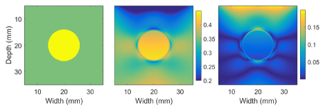
Eigenstrain is added to consider the variation of total strain from the elastic one in the presence of inhomogeneity. It is maximum on the inhomogeneity boundaries and decays to zero further from the boundaries [48]. Although the lateral strain does not linearly depend on the axial one anymore, they are still highly correlated. Also, $-\varepsilon_{22}/\varepsilon_{11}$ does not obtain the Poisson’s ratio anymore and it is called Effective Poisson’s ratio (EPR) [44]. In uniform regions far from inhomogeneities, EPR converges to Poisson’s ratio. For illustration purpose, EPR and Poisson’s ratio of a finite element simulation using ABAQUS software (Providence, RI) is depicted in Fig. 1. It can be observed that EPR is more dissimilar to Poisson’s ratio at the top and bottom of the phantom and around the inclusion. Poisson’s ratio and EPR under arbitrary deformation have the range between 0.2 and 0.5 [49, 50]. Although the exact value of EPR is not known, it has been used as an approximation of Poisson’s ratio to characterize tissues [44, 50]. We propose to use this range as a prior information to guide the network to refine the lateral displacement. Guo et al. assumed tissue incompressibility (Poisson’s ratio = 0.5) and plane strain (strain in out-of-plane direction = 0) to refine the displacements. However, Poisson’s ratio depends on the type of the tissue (refer to [51, 52] for Poisson’s ratio of breast and liver). In this work, we do not make those assumptions, and only a feasible range of Poisson’s ratio is enforced.

Figure 1: From left to right: the Poisson’s ratio, the EPR, and their absolute difference for a simulated phantom. The Poisson’s ratio and the EPR have the same colorbar.

2.3 PICTURE

We propose to utilize the accepted range of EPR as a prior information in the form of regularization. To do that, we first need to calculate EPR ($V_{e}$) from the estimated axial and lateral strains:

$$V_{e}=\frac{-\tilde{\varepsilon_{22}}}{\mathbf{S}(\tilde{\varepsilon_{11}})}$$ (7)

where $\tilde{\varepsilon_{22}}$ and $\tilde{\varepsilon_{11}}$ are the lateral and axial strains obtained from estimated displacements. The parameter $\mathbf{S}$ denotes stop gradient operation, which is used to stop backpropagation of the loss to the axial displacement estimation. It is used to avoid the estimated axial displacement being altered by the noisy lateral one. To find out the EPR values outside the accepted range, a mask ($M$) is defined using the minimum ($V_{emin}$) and maximum ($V_{emax}$) allowed EPR values.

$$M(i,j)=\begin{Bmatrix}0&&V_{emin}<V_{e}(i,j)<V_{emax}\\ 1&&otherwise\\ \end{Bmatrix}$$ (8)

We assume the $V_{emin}$ and $V_{emax}$ values to be 0.1 and 0.6 (no noticeable change was observed by small changes of these values) to have a small margin of error. In order to penalize the EPR values outside of the accepted range, PICTURE loss is defined as:

$$\begin{gathered}L_{vd}=\left|\left|M\otimes(\tilde{\varepsilon_{22}}+\bar{V_{e}}\times\mathbf{S}(\tilde{\varepsilon_{11}}))\right|\right|_{2}\end{gathered}$$ (9)

where $\otimes$ is the Kronecker product to select EPR values outside the accepted range, and $\bar{V_{e}}$ is an estimate of true average EPR. It is obtained by averaging EPR values that are inside the accepted range, which can be formulated as:

$$\bar{V_{e}}=\frac{\sum_{i,j}(1-M_{(i,j)})V_{e}(i,j)}{\sum_{i,j}(1-M_{(i,j)})}$$ (10)

Eq 9 tries to constrain EPR to be inside the accepted range.

The first-order derivatives of $V_{e}$ are also employed to enforce the smoothness of EPR.

$$L_{vs}=||\frac{\partial V_{e}}{\partial a}||_{1}+\beta\times||\frac{\partial V_{e}}{\partial l}||_{1}$$ (11)

The final PICTURE loss can be written as:

$$L_{V}=L_{vd}+\lambda_{vs}\times L_{vs}$$ (12)

where $\lambda_{vs}$ is defined to weight the smoothness part.

2.4 Self-Supervised Learning

Self-supervised learning (SSL) is a technique that has recently been applied to unsupervised optical flow networks [53, 54]. The basic procedure is that the input images are fed to the network during the unsupervised training, and the displacements are obtained during the first pass. In the next step, the input images are transformed to make them more challenging than before and the new displacement is obtained during the second pass. In the last step, the differences between the displacements of the first and second passes are penalized:

$$L_{SSL}=||\mathbf{S}(W)-\tilde{W}||_{1}$$ (13)

where $W$ is the estimated displacement in the first pass (no transformation), $\tilde{W}$ is the obtained displacement from the second pass (with transformed inputs), and stop gradient ($\mathbf{S}$) is used to avoid backpropagation into the first pass. Substantial improvements were reported for unsupervised training employing SSL using different transformations. In [54], superpixels [55] of input images were identified and the content of randomly selected superpixels were replaced by pure noise. The method outperformed other unsupervised methods in different optical flow benchmarks. In [53], cropping, affine, and other kinds of transformations were utilized. SSL was also compared by data augmentation (instead of SSL, the transformed images were considered as new inputs). SSL outperformed data augmentation, which indicated that SSL was not a simple synthetic data generation like data augmentation.

Figure 2: B-mode input image (a), cropped image (resized for the purpose of visualization) (b) and, image with added noise (the area of added noise is highlighted) (c).

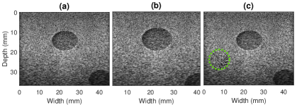
In this paper, we employ two data transformations: cropping and adding noise to specific regions. Cropping may cause loss of information, especially in areas where displacement is high. On those areas, estimating displacement is complex for the network since the corresponding part of the first image might be outside the cropped second image. We also add large Gaussian noise to randomly selected circular regions. An example of a transformed image is shown in Fig. 2. SSL can guide the network to have a more reliable estimation when there is a loss of information due to cropping or noisy data.

2.5 Loss Function And Network Architecture

The loss function is composed of data loss (Eq 1), smoothness loss (Eq 3), PICTURE loss (Eq 9), and SSL regularization (Eq 13):

$$loss=\underbrace{L_{D}+\lambda_{s}L_{S}+\lambda_{v}L_{V}}_{first\ pass}+\underbrace{\lambda_{sl}L_{SSL}}_{second\ pass}$$ (14)

where the hyper-parameters, $\lambda_{s}$, $\lambda_{v}$, and $\lambda_{sl}$ are the weights of smoothness regularization, PICTURE loss, and SSL regularization, respectively. The SSL loss only affects the second pass in which the input US data are transformed, while the other losses affect the first pass.

We employed MPWC-Net++ [28] as the network. This network has demonstrated promising results on USE by increasing the search range of correlation layers and reducing the downsampling of PWC-Net-IRR [30] feature extraction layers. The modification necessitated training the network from scratch; therefore, the FlyingChairsOcc dataset [30] with 23000 image pairs was employed for the training. Refer to [28] for more details about the architecture of this network. The network’s weights are publicly available online at code.sonography.ai.

The hyperparameters values used for the training of unsupervised method and sPICTURE are given in the Supplementary Materials. The networks are trained for 25 epochs, the learning rate is set to $5\times 10^{-6}$, which is halved every 5 epochs.

Figure 3: Axial (top row) and lateral (middle row) strains in a simulated phantom. Ground truth EPR (bottom row), the absolute error, and the mean absolute error (MAE) shown for each method.

2.6 Datasets

2.6.1 Simulation data

A phantom is simulated using Field II [56, 57], and the motion is obtained by the ABAQUS finite element analysis software (Providence, RI). The phantom contains an inclusion with Poisson’s ratio of 0.45 and the Young’s modulus of 40 kPa. The background has Poisson’s ratio of 0.35 and the Young’s modulus of 21 kPa. The Poisson’s ratio and EPR of this phantom are shown in Fig. 1. Different Poisson’s ratios for background and the inclusion are chosen to investigate if it is detectable by the networks. Compared to our recent simulation dataset [27], the number of lines in FIELD II is increased to 190, the number of active elements is increased to 96, and the obtained US images are also upsampled in the lateral direction by 2 to provide high lateral resolution.

In addition, 1200 pairs of publicly available simulated phantoms from [27] are employed for training and 70 pairs for quantitative evaluation of the compared methods. These phantoms have a Poisson’s ratio of 0.49 and have one or two hard inclusions in different locations. The Young’s modulus for the background and inclusions are around 20 kPa and 45-60 kPa, respectively.

2.6.2 Experimental phantom data

RF data is collected from a tissue-mimicking breast phantom (Model 059, CIRS: Tissue Simulation & Phantom Technology, Norfolk, VA) at Concordia University. It has Young’s modulus of 20 kpa and contains several inclusions with the Young’s modulus of at least 40 kPa. We employed an Alpinion E-Cube R12 research US machine (Bothell, WA, USA) for data collection. The sampling frequency was 40 MHz and the center frequency was 8 MHz. We made this data publicly available online at code.sonography.ai in [34].

2200 frame pairs are employed for training of the network. In order to avoid data leakage, different parts of the phantom were imaged for evaluation and test.

2.6.3 in vivo data

Data were acquired from patients with liver cancer during open-surgical RF thermal ablation at Johns Hopkins Hospital. A research Antares Siemens system by a VF 10-5 linear array was used for data collection. The sampling and center frequencies were 40 MHz and 6.67 MHz, respectively. The study was approved by the institutional review board with the consent of all patients. 500 RF frame pairs from after ablation were selected for the training of the networks, and RF data from 2 patients before ablations were employed for test to prevent using similar data during the train and test phases.

2.7 Quantitative Metrics

Mean Absolute Error (MAE) and Structural Similarity Index Metric (SSIM) [58] are employed for simulation results where the ground truth is available. For experimental phantoms, Contrast to Noise Ratio (CNR), and Strain Ratio (SR) are reported [1]:

$$CNR=\sqrt{\frac{2(\overline{s}_{b}-\overline{s}_{t})^{2}}{{\sigma_{b}}^{2}+{\sigma_{t}}^{2}}},\quad\quad SR=\frac{\overline{s}_{t}}{\overline{s}_{b}},$$ (15)

where $\overline{s}_{X}$, and ${\sigma_{X}}$ are the mean and the standard deviation of obtained strain in the target (subscript $t$) and background (subscript $b$) windows. Assuming that the target is stiffer than the background, lower SR represents a higher difference between the average of strain in the target and background windows. In SR, the mean values of strains are employed; therefore, it is insensitive to the variance of strains. CNR combines both the mean and variance of the target and background windows which can provide a good intuition of the overall quality of the strain image.

Table 1: Quantitative results for 70 simulated phantoms. Mean and standard deviation ($\pm$) of the MAE of displacements and SSIM of strains are reported. The pairs marked by asterisk are not statistically significant (p-value$>$0.05, using Friedman test).

	Axial		Lateral
	MAE $(\mu m)$	SSIM $(\%)$	MAE $(\mu m)$	SSIM $(\%)$
[HTML]C0C0C0 SOUL	2.2$\pm$1.5	99.80$\pm$0.06	8.00$\pm$4.1∗	97.70 $\pm$ 1.56∗
OVERWIND	2.2$\pm$1.5	99.80$\pm$0.07	9.40$\pm$4.6	93.48$\pm$4.10
[HTML]C0C0C0 Unsupervised	2.7$\pm$1.6∗	99.43 $\pm$ 2.10	8.70$\pm$4.1	96.42$\pm$1.79
sPICTURE	2.7$\pm$1.7∗	99.55 $\pm$ 1.80	8.00$\pm$3.8∗	97.73 $\pm$1.29∗

Figure 4: The experimental phantom lateral strains obtained by the evaluated methods. The target and background windows for calculation of CNR and SR are marked in the B-mode images. The corresponding axial strains are shown in the supplementary video. The samples 1, 2 and 3 are taken from different locations of the tissue-mimicking breast phantom. Hard inclusions have lower absolute values than the background.

3 Results

The evaluated methods are listed below:

• Second-Order Ultrasound Elastography (SOUL) is an optimization-based method which employs L2-norm and second-order regularization to have smooth strain images with high target-background contrast [13].

• Total Variation Regularization and Window-based time delay estimation (OVERWIND) is a method that incorporate windowing into the optimization cost function [12].

• Unsupervised method ($\lambda_{v}=0$ and $\lambda_{sl}=0$ in Eq 14, similar to the unsupervised method in [34]).

• The PICTURE without SSL ($\lambda_{sl}=0$ in Eq 14, only used in ablation experiment).

• The proposed method named sPICTURE entails both PICTURE and SSL losses (Eq 14).

It should be mentioned that for simulation results the network for unsupervised method and sPICTURE is trained on simulation data. For the experimental phantom results, it is trained on the experimental phantom dataset, and for in vivo results, it is trained on the available in vivo dataset. We also tuned the hyperparameters of the optimization-based methods (SOUL and OVERWIND) for each dataset separately to ensure that the best results are obtained from those methods.

3.1 Simulation Results

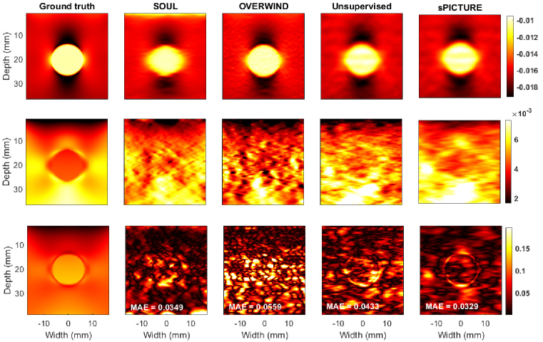
The axial, lateral strains, and the EPR of the simulated phantom obtained by the compared methods are illustrated in Fig. 3. All methods obtain high-quality axial strains. The axial strain of the unsupervised method and sPICTURE are quite similar since PICTURE is only applied to the lateral displacement and keep the axial one untouched. Comparing the lateral strains (second row), sPICTURE reduces the noise presented in the unsupervised method.

The mean and standard deviations of quantitative metrics are reported for 70 simulated phantoms. Since the ground truth is available, MAE of displacement and SSIM of strain are reported for the axial and lateral displacements and strains. SOUL and OVERWIND have the lowest MAE error and highest SSIM in the axial direction. sPICTURE performs similar to the unsupervised method since PICTURE does not affect the axial direction. In lateral displacement estimation, sPICTURE reduces the lateral MAE of unsupervised method from 25.0 to 7.9, a decrease of more than three folds. It also outperforms the optimization-based methods in terms of MAE, with SSIM values close to those of SOUL.

3.1.1 simulation results for different signal to noise ratios (SNR)

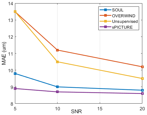
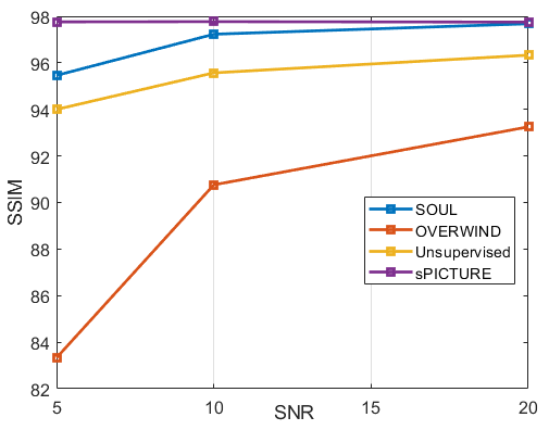
Random Gaussian noise with different SNRs is added to the test RF data to evaluate the robustness of the compared method to noise. MAE of lateral displacement and SSIM of lateral strain are plotted in Fig. 5. It can be observed that sPICTURE has a low MAE even for an SNR as low as 5 dB which demonstrates the high robustness of this method.

Figure 5: MAE of lateral displacements (left), and SSIM of lateral strains (right) for different SNR values of simulation test data.

3.1.2 simulation results for different compression

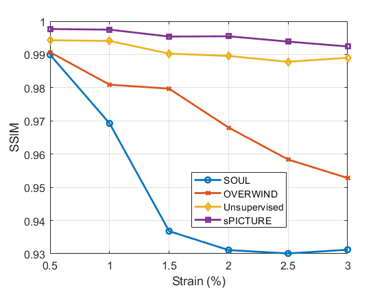
A phantom from simulation test data having different applied compressions, resulting in different maximum strains, is selected, and SSIM of lateral strain are illustrated in Fig. 6. By increasing the maximum strain, the SSIM of all compared method decreased which is expected. It should be noted that the graph shows that sPICTURE has the highest SSIM among the compared methods which is also robust to the variations of applied compression.

Figure 6: SSIM of lateral strains versus different maximum strains.

3.2 Experimental Phantom Results

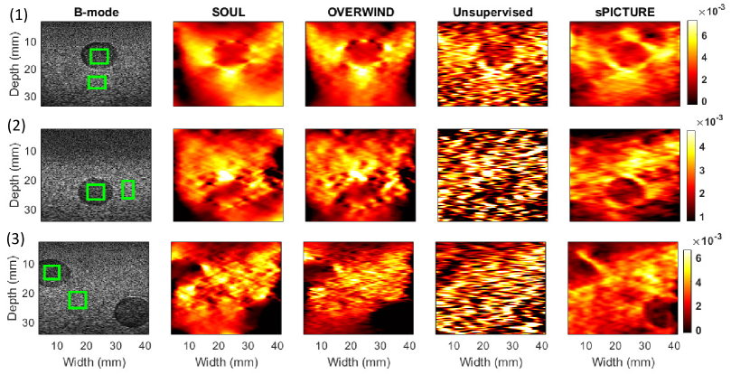
The lateral strains of experimental phantom results are shown in Fig 4 and the quantitative results are reported in Table 2.

Figure 7: The histograms of the EPR of different methods for phantom 3. sPICTURE has limited the EPR to the feasible range for USE.

Figure 8: Ablation experiment results. In (3), the inclusion is not visible in B-mode image and arrows show that SSL improves the estimation in boundary regions. The samples 1, 2 and 3 are taken from different locations of the tissue-mimicking breast phantom.

Figure 9: Normalized axial strain versus the corresponding lateral strain. The region where the samples of the methods lie for experimental phantom 2 are specified. The regions are obtained from convex hull of strain samples. EPR equals to 0.1 and 0.6 are highlighted by the dashed lines.

Figure 10: The in vivo lateral strains obtained by the evaluated methods. The target and background windows for calculation of CNR and SR are marked in the B-mode images. The corresponding axial strains are given in the Supplementary Materials.

Figure 11: Lateral strains of OVERWIND and sPICTURE after applying the method of Guo et al. [39] to real phantom data (1).

Table 2: Quantitative results of lateral strains for experimental phantoms and in vivo data. Mean and standard deviation ($\pm$) of CNR (higher is better) and SR (lower is better) of lateral strains are reported. The pair marked by asterisk is not statistically significant (p-value$>$0.05, using Friedman test).

	Phantom 1		Phantom 2		Phantom 3		In vivo 1		In vivo 2
	CNR	[HTML]C0C0C0SR	CNR	[HTML]C0C0C0SR	CNR	[HTML]C0C0C0SR	CNR	[HTML]C0C0C0SR	CNR	[HTML]C0C0C0SR
SOUL	11.01$\pm$4.52	[HTML]C0C0C00.483$\pm$0.038	3.63$\pm$1.20	[HTML]C0C0C00.676$\pm$0.081∗	2.33$\pm$0.81	[HTML]C0C0C00.327$\pm$0.140	3.25$\pm$1.07	[HTML]C0C0C0 0.428$\pm$0.137	1.26$\pm$ 0.843	[HTML]C0C0C0 1.110$\pm$0.124
OVERWIND	7.21$\pm$1.91	[HTML]C0C0C00.456$\pm$0.057	2.35$\pm$0.68	[HTML]C0C0C00.676$\pm$0.092∗	3.38$\pm$1.45	[HTML]C0C0C00.285$\pm$0.155	1.92$\pm$0.96	[HTML]C0C0C00.584$\pm$0.150	0.84$\pm$0.61	[HTML]C0C0C0 1.048$\pm$0.202
Unsupervised	2.31$\pm$0.30	[HTML]C0C0C00.454$\pm$0.061	1.02$\pm$0.30	[HTML]C0C0C00.530$\pm$0.105	0.26$\pm$0.18	[HTML]C0C0C00.677$\pm$0.743	0.24$\pm$0.18	[HTML]C0C0C00.905$\pm$0.159	0.50$\pm$0.36	[HTML]C0C0C0 1.125 $\pm$ 0.437
sPICTURE	11.20$\pm$2.18	[HTML]C0C0C00.511$\pm$0.059	9.14$\pm$2.80	[HTML]C0C0C00.527$\pm$0.044	7.07$\pm$1.76	[HTML]C0C0C00.278$\pm$0.065	7.80$\pm$2.01	[HTML]C0C0C00.242$\pm$0.066	4.34$\pm$1.39	[HTML]C0C0C0 0.640$\pm$0.075

Unsupervised method has unacceptable results in which the inclusions are not visually detectable while it provides high-quality axial strain images (the axial strain images are shown in the Supplementary Materials) comparable to optimization-based methods. This is an important observation since this shows that the unsupervised loss (composed of data and smoothness losses), which has been used widely in computer vision optical flow estimation, is not a suitable loss in USE.

sPICTURE provides high-quality lateral strain images and performs the best in terms of quantitative results among the compared methods. By comparing the unsupervised and sPICTURE results, it can be seen how the added PICTURE regularization and the SSL lead to the improvement of the obtained strain images. The added regularizations convert the unreliable and noisy lateral strains obtained by unsupervised method to the high-quality strain images. It should be mentioned that sPICTURE and unsupervised methods are both trained using the same data and weights for smoothness regularization. Furthermore, sPICTURE obtains substantially higher quality lateral strain images than the compared optimization-based methods (both visually and quantitatively).

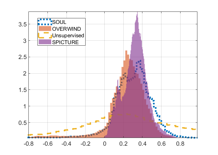
To further analyze the results, the histograms of the EPR of phantom data 3 are depicted in Fig. 7. As mentioned earlier, EPR range is similar to the Poisson’s ratio range (0.2 to 0.5, excluding the boundary regions). In PICTURE loss, we penalize EPR values outside the 0.1-0.6 range. The histogram of EPR of unsupervised method covers a wide range of positive and negative values which indicates that many lateral strain values obtained by this method are incorrect. The histogram of the EPR values of OVERWIND and SOUL are more limited than unsupervised method, but they contain values that are negative or higher than 0.8 which is not possible in the phantom. sPICTURE has a more limited range of EPR values but still has some values outside the specified range. The reason is that the proposed PICTURE regularization is only applied during the training phase. Although the proposed PICTURE regularization reduces the range of EPR values, it does not guarantee that all the values fall into the specified range in test time.

3.2.1 Ablation Experiment

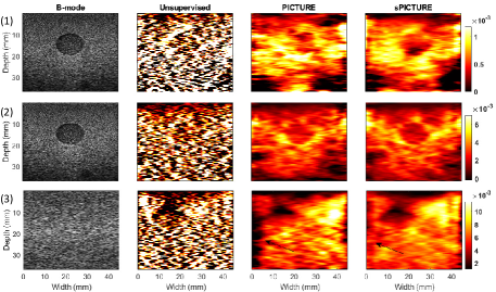
In order to investigate the impact of PICTURE loss and SSL separately, an ablation experiment is conducted. Fig. 8 shows the visual comparison of unsupervised method (without PICTURE and SSL), PICTURE (without SSL), and sPICTURE. It is visually clear that both PICTURE and SSL contribute to the improvements obtained by sPICTURE. Without PICTURE, unsupervised method provides noisy and impractical lateral strain images. PICTURE substantially improves the lateral strain image quality and SSL further boosts the quality of the lateral strain image. For instance, in sample (1), the inclusion location can be detected more accurately in sPICTURE compared to PICTURE. Also, the estimation in boundary regions is improved in sPICTURE since it is trained to deal with cropping with SSL. It should be mentioned that SSL without PICTURE was also tested, but it performed inferior to PICTURE.

3.2.2 Experimental Results after applying lateral displacement refinement

Lateral displacement refinement of Guo et al. [39] is applied using the initial displacement obtained by OVERWIND and sPICTURE. It can be observed that this method further improves the lateral displacement estimation, and the initial displacement obtained by sPICTURE provides a high-quality initial value for this method.

3.3 In vivo Results

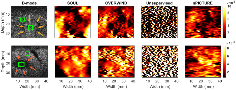
The in vivo lateral strains of two patients with liver cancer are depicted in Fig. 10, quantitative results are reported in Table 2, and their corresponding axial strains are given in the Supplementary Materials. The tumors are more visually detectable in sPICTURE compared to the other methods. Also, quantitative results denote that sPICTURE has the highest CNR and lowest SR values among the compared methods, which confirms the visual analysis.

4 Discussion

In this paper, a physically inspired regularization to improve the lateral displacement estimation has been proposed. It confines the range of EPR by employing the high-quality axial strain and the known range of EPR values. One limitation of the proposed method is that PICTURE similar to any other form of regularizations is only applied during the training. Even though it limits the range of EPR values in the test time, it does not guarantee that all EPR values be within that range. We observed only a few samples lie outside of the defined range and fixing them during the test time inspired by known operators [59] can be an area of future works.

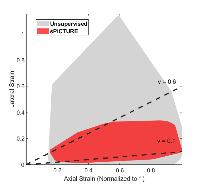
It should be mentioned that PICTURE can also have statistical interpretation. The lateral displacement prediction can be viewed as the estimation of a parameter from under sampled and heavily smoothed observations. The conventional methods estimate this parameter in a maximum likelihood (ML) manner without any prior information (only smoothness is considered). However, PICTURE can be viewed as maximum a posteriori (MAP) estimate in which the prior information from compression physics is utilized to find the parameters. Therefore, more reliable lateral displacement can be estimated compared to the conventional methods. To clarify this, the graph of lateral versus axial strains is depicted in Fig. 9. PICTURE enforced the strain samples to lie within $v=0.6$ and $v=0.1$. The areas where the samples of unsupervised method and sPICTURE lie for experimental phantom data 2 are illustrated in the figure. It can be observed that most of the strain samples of sPICTURE lie within the correct range. sPICTURE moved the lateral sample values to the area of the prior knowledge.

Self-supervision was another regularization that has been used in this work. SSL can prepare the model to deal with corrupted data. In this paper, we applied cropping and added noise. Cropping helps the model deal with boundary regions where finding the correspondence between pre and post-compression images is difficult. Adding noise can also be useful in some scenarios for instance when there is a loss of signal due to high attenuation or there is a cyst where clutter is stronger than the true signal. Applying other forms of transformation such as acoustic noise (reverberation and multiple scattering), inducing decorrelation, and downsampling can be an area of future works.

In this paper, the performance of lateral displacement refinement method of [39] using initial value from sPICTURE and OVERWIND is also investigated. This method is considered as a post-processing method that relies on the initial displacements. We showed that high-quality lateral displacement of sPICTURE can be considered as a good initial value for this method and improves the results of this refinement method.

Complexity of the training is another issue that should be discussed. We utilized two parallel NVIDIA A100 GPUs with 40 GB of memory each. Even with this size of memory, the maximum batch size that we could train the network was 8. The main reason is that the image sizes are usually large to preserve high-frequency RF data contents and the memory usage is also doubled by the second pass introduced required in SSL. Only the training phase is memory intensive, and inference can be performed with only 5 GB of memory in 140 $ms$ (for an US data of size $2048\times 256$) similar to MPWC-Net++.

5 Conclusion

In this paper, we proposed PICTURE to improve the lateral strain images in USE using physically inspired priors. We further improved the method in sPICTURE by adding the self-supervision to the method. The effectiveness of the proposed method is validated using simulation, experimental phantom, and in vivo data.

6 Acknowledgment

This work is Supported by Natural Sciences and Engineering Research Council of Canada (NSERC) Discovery Grant. The Alpinion ultrasound machine was partly funded by Dr. Louis G. Johnson Foundation. The authors would like to thank Drs. E. Boctor, M. Choti and G. Hager for providing us with the in vivo patients data from Johns Hopkins Hospital.

References

- [1] J. Ophir, S. K. Alam, B. Garra, F. Kallel, E. Konofagou, T. Krouskop, and T. Varghese, “Elastography: ultrasonic estimation and imaging of the elastic properties of tissues,” Proceedings of the Institution of Mechanical Engineers, Part H: Journal of Engineering in Medicine, vol. 213, no. 3, p. 203–233, 1999.
- [2] T. Varghese, E. Konofagou, J. Ophir, S. Alam, and M. Bilgen, “Direct strain estimation in elastography using spectral cross-correlation,” Ultrasound in medicine & biology, vol. 26, no. 9, p. 1525–1537, 2000.
- [3] A. Kling and J. Jiang, “Potential of determining thermal dose for ablation therapies using ultrasound elastography: An ex vivo feasibility study,” in 2018 IEEE International Ultrasonics Symposium (IUS). IEEE, 2018, p. 1–4.
- [4] F.-F. Lee, Q. He, J. Gao, A. Pan, S. Sun, X. Liang, and J. Luo, “Evaluating hifu-mediated local drug release using thermal strain imaging: Phantom and preliminary in-vivo studies,” Medical physics, 2019.
- [5] A. Lyshchik, T. Higashi, R. Asato, S. Tanaka, J. Ito, J. J. Mai, C. Pellot-Barakat, M. F. Insana, A. B. Brill, T. Saga, M. Hiraoka, and K. Togashi, “Thyroid gland tumor diagnosis at us elastography,” Radiology, vol. 237, no. 1, pp. 202–211, 2005, pMID: 16118150. [Online]. Available: https://doi.org/10.1148/radiol.2363041248
- [6] T. J. Hall, Y. Zhu, C. S. Spalding, and L. T. Cook, “In vivo results of real-time freehand elasticity imaging,” in 2001 IEEE Ultrasonics Symposium. Proceedings. An International Symposium (Cat. No. 01CH37263), vol. 2. IEEE, 2001, p. 1653–1657.
- [7] A. Nahiyan and M. K. Hasan, “Hybrid algorithm for elastography to visualize both solid and fluid-filled lesions,” Ultrasound in medicine & biology, vol. 41, no. 4, p. 1058–1078, 2015.
- [8] J. Luo and E. E. Konofagou, “A fast normalized cross-correlation calculation method for motion estimation,” IEEE transactions on ultrasonics, ferroelectrics, and frequency control, vol. 57, no. 6, p. 1347–1357, 2010.
- [9] J. Jiang and T. J. Hall, “A parallelizable real-time motion tracking algorithm with applications to ultrasonic strain imaging,” Physics in Medicine & Biology, vol. 52, no. 13, p. 3773, 2007.
- [10] M. Mirzaei, A. Asif, M. Fortin, and H. Rivaz, “3d normalized cross-correlation for estimation of the displacement field in ultrasound elastography,” Ultrasonics, vol. 102, p. 106053, 2020.
- [11] H. S. Hashemi and H. Rivaz, “Global time-delay estimation in ultrasound elastography,” IEEE transactions on ultrasonics, ferroelectrics, and frequency control, vol. 64, no. 10, p. 1625–1636, 2017.
- [12] M. Mirzaei, A. Asif, and H. Rivaz, “Combining total variation regularization with window-based time delay estimation in ultrasound elastography.” IEEE transactions on medical imaging, 2019.
- [13] M. Ashikuzzaman, A. Sadeghi-Naini, A. Samani, and H. Rivaz, “Combining first and second order continuity constraints in ultrasound elastography,” IEEE Transactions on Ultrasonics, Ferroelectrics, and Frequency Control, 2021.
- [14] I. N. Fleming, “Robust displacement estimation for ultrasound elastography and thermal imaging,” Ph.D. dissertation, Johns Hopkins University, 2014.
- [15] M. McCormick, N. Rubert, and T. Varghese, “Bayesian regularization applied to ultrasound strain imaging,” IEEE transactions on biomedical engineering, vol. 58, no. 6, pp. 1612–1620, 2011.
- [16] M. G. Kibria and H. Rivaz, “Gluenet: Ultrasound elastography using convolutional neural network,” in Simulation, Image Processing, and Ultrasound Systems for Assisted Diagnosis and Navigation. Springer, 2018, p. 21–28.
- [17] S. Wu, Z. Gao, Z. Liu, J. Luo, H. Zhang, and S. Li, “Direct reconstruction of ultrasound elastography using an end-to-end deep neural network,” in International Conference on Medical Image Computing and Computer-Assisted Intervention. Springer, 2018, p. 374–382.
- [18] Z. Gao, S. Wu, Z. Liu, J. Luo, H. Zhang, M. Gong, and S. Li, “Learning the implicit strain reconstruction in ultrasound elastography using privileged information,” Medical image analysis, vol. 58, p. 11–18, 2019.
- [19] B. Peng, Y. Xian, and J. Jiang, “A convolution neural network-based speckle tracking method for ultrasound elastography,” in 2018 IEEE International Ultrasonics Symposium (IUS). IEEE, 2018, p. 206–212.
- [20] E. Evain, K. Faraz, T. Grenier, D. Garcia, M. De Craene, and O. Bernard, “A pilot study on convolutional neural networks for motion estimation from ultrasound images,” IEEE transactions on ultrasonics, ferroelectrics, and frequency control, vol. 67, no. 12, pp. 2565–2573, 2020.
- [21] B. Peng, Y. Xian, Q. Zhang, and J. Jiang, “Neural-network-based motion tracking for breast ultrasound strain elastography: An initial assessment of performance and feasibility,” Ultrasonic imaging, vol. 42, no. 2, pp. 74–91, 2020.
- [22] A. K. Tehrani, M. Amiri, and H. Rivaz, “Real-time and high quality ultrasound elastography using convolutional neural network by incorporating analytic signal,” in 2020 42nd Annual International Conference of the IEEE Engineering in Medicine & Biology Society (EMBC). IEEE, 2020, pp. 2075–2078.
- [23] A. Zayed and H. Rivaz, “Fast strain estimation and frame selection in ultrasound elastography using machine learning,” IEEE transactions on ultrasonics, ferroelectrics, and frequency Control, vol. 68, no. 3, pp. 406–415, 2020.
- [24] N. Mohammadi, M. M. Doyley, and M. Cetin, “Combining physics-based modeling and deep learning for ultrasound elastography,” in 2021 IEEE International Ultrasonics Symposium (IUS). IEEE, 2021, pp. 1–4.
- [25] D. Y. Chan, D. C. Morris, T. J. Polascik, M. L. Palmeri, and K. R. Nightingale, “Deep convolutional neural networks for displacement estimation in arfi imaging,” IEEE Transactions on Ultrasonics, Ferroelectrics, and Frequency Control, vol. 68, no. 7, pp. 2472–2481, 2021.
- [26] E. Evain, Y. Sun, K. Faraz, D. Garcia, E. Saloux, B. L. Gerber, M. De Craene, and O. Bernard, “Motion estimation by deep learning in 2d echocardiography: synthetic dataset and validation,” IEEE transactions on medical imaging, 2022.
- [27] A. K. Tehrani and H. Rivaz, “Displacement estimation in ultrasound elastography using pyramidal convolutional neural network,” IEEE transactions on ultrasonics, ferroelectrics, and frequency control, vol. 67, no. 12, pp. 2629–2639, 2020.
- [28] A. K.Z. Tehrani and H. Rivaz, “Mpwc-net++: evolution of optical flow pyramidal convolutional neural network for ultrasound elastography,” in Medical Imaging 2021: Ultrasonic Imaging and Tomography, vol. 11602. International Society for Optics and Photonics, 2021, p. 1160206.
- [29] D. Sun, X. Yang, M.-Y. Liu, and J. Kautz, “Pwc-net: Cnns for optical flow using pyramid, warping, and cost volume,” in Proceedings of the IEEE Conference on Computer Vision and Pattern Recognition, 2018, p. 8934–8943.
- [30] J. Hur and S. Roth, “Iterative residual refinement for joint optical flow and occlusion estimation,” in Proceedings of the IEEE/CVF Conference on Computer Vision and Pattern Recognition, 2019, pp. 5754–5763.
- [31] R. Delaunay, Y. Hu, and T. Vercauteren, “An unsupervised approach to ultrasound elastography with end-to-end strain regularisation,” in International Conference on Medical Image Computing and Computer-Assisted Intervention. Springer, 2020, pp. 573–582.
- [32] R. Delaunay, Y. Hu, and T. Vercauteren, “An unsupervised learning approach to ultrasound strain elastography with spatio-temporal consistency,” Physics in Medicine & Biology, 2021.
- [33] A. K. Tehrani, M. Mirzaei, and H. Rivaz, “Semi-supervised training of optical flow convolutional neural networks in ultrasound elastography,” in International Conference on Medical Image Computing and Computer-Assisted Intervention. Springer, 2020, pp. 504–513.
- [34] A. K. Tehrani, M. Sharifzadeh, E. Boctor, and H. Rivaz, “Bi-directional semi-supervised training of convolutional neural networks for ultrasound elastography displacement estimation,” IEEE Transactions on Ultrasonics, Ferroelectrics, and Frequency Control, 2022.
- [35] X. Wei, Y. Wang, L. Ge, B. Peng, Q. He, R. Wang, L. Huang, Y. Xu, and J. Luo, “Unsupervised convolutional neural network for motion estimation in ultrasound elastography,” IEEE Transactions on Ultrasonics, Ferroelectrics, and Frequency Control, 2022.
- [36] M. Ashikuzzaman and H. Rivaz, “Second-order ultrasound elastography with l1-norm spatial regularization,” IEEE Transactions on Ultrasonics, Ferroelectrics, and Frequency Control, 2022.
- [37] S. Zhao, Y. Sheng, Y. Dong, E. I. Chang, Y. Xu et al., “Maskflownet: Asymmetric feature matching with learnable occlusion mask,” in Proceedings of the IEEE/CVF Conference on Computer Vision and Pattern Recognition, 2020, pp. 6278–6287.
- [38] O. A. Babaniyi, A. A. Oberai, and P. E. Barbone, “Recovering vector displacement estimates in quasistatic elastography using sparse relaxation of the momentum equation,” Inverse problems in science and engineering, vol. 25, no. 3, pp. 326–362, 2017.
- [39] L. Guo, Y. Xu, Z. Xu, and J. Jiang, “A pde-based regularization algorithm toward reducing speckle tracking noise: A feasibility study for ultrasound breast elastography,” Ultrasonic imaging, vol. 37, no. 4, pp. 277–293, 2015.
- [40] Y. Wang, X. Xie, Q. He, H. Liao, H. Zhang, and J. Luo, “Hadamard-encoded synthetic transmit aperture imaging for improved lateral motion estimation in ultrasound elastography,” IEEE Transactions on Ultrasonics, Ferroelectrics, and Frequency Control, vol. 69, no. 4, pp. 1204–1218, 2022.
- [41] M. Mirzaei, A. Asif, and H. Rivaz, “Virtual source synthetic aperture for accurate lateral displacement estimation in ultrasound elastography,” IEEE Transactions on Ultrasonics, Ferroelectrics, and Frequency Control, vol. 68, no. 5, pp. 1687–1695, 2020.
- [42] S. Selladurai and A. K. Thittai, “Strategies to obtain subpitch precision in lateral motion estimation in ultrasound elastography,” IEEE transactions on ultrasonics, ferroelectrics, and frequency control, vol. 65, no. 3, pp. 448–456, 2018.
- [43] N. Mohammadi, M. M. Doyley, and M. Cetin, “Ultrasound elasticity imaging using physics-based models and learning-based plug-and-play priors,” in ICASSP 2021-2021 IEEE International Conference on Acoustics, Speech and Signal Processing (ICASSP). IEEE, 2021, pp. 1165–1169.
- [44] M. T. Islam, A. Chaudhry, S. Tang, E. Tasciotti, and R. Righetti, “A new method for estimating the effective poisson’s ratio in ultrasound poroelastography,” IEEE transactions on medical imaging, vol. 37, no. 5, p. 1178–1191, 2018.
- [45] A. KZ Tehrani and H. Rivaz, “Physically inspired constraint for unsupervised regularized ultrasound elastography,” in International Conference on Medical Image Computing and Computer-Assisted Intervention. Springer, 2022, pp. 218–227.
- [46] S. Meister, J. Hur, and S. Roth, “Unflow: Unsupervised learning of optical flow with a bidirectional census loss,” in Proceedings of the AAAI Conference on Artificial Intelligence, vol. 32, no. 1, 2018.
- [47] A. C. Ugural and S. K. Fenster, Advanced strength and applied elasticity. Pearson education, 2003.
- [48] L. Ma and A. M. Korsunsky, “The principle of equivalent eigenstrain for inhomogeneous inclusion problems,” International Journal of Solids and Structures, vol. 51, no. 25-26, pp. 4477–4484, 2014.
- [49] P. Mott and C. Roland, “Limits to poisson’s ratio in isotropic materials—general result for arbitrary deformation,” Physica Scripta, vol. 87, no. 5, p. 055404, 2013.
- [50] R. Righetti, J. Ophir, S. Srinivasan, and T. A. Krouskop, “The feasibility of using elastography for imaging the poisson’s ratio in porous media,” Ultrasound in medicine & biology, vol. 30, no. 2, pp. 215–228, 2004.
- [51] D. George, M. Baniassadi, Y. Hoarau, M. Kugler, and Y. Rémond, “Influence of the liver vascular distribution on its overall mechanical behavior: a first approach to multiscale fluid-structure homogenization,” Journal of Cellular Immunotherapy, vol. 4, no. 1, pp. 35–37, 2018.
- [52] R. H. Griesenauer, J. A. Weis, L. R. Arlinghaus, I. M. Meszoely, and M. I. Miga, “Breast tissue stiffness estimation for surgical guidance using gravity-induced excitation,” Physics in Medicine & Biology, vol. 62, no. 12, p. 4756, 2017.
- [53] L. Liu, J. Zhang, R. He, Y. Liu, Y. Wang, Y. Tai, D. Luo, C. Wang, J. Li, and F. Huang, “Learning by analogy: Reliable supervision from transformations for unsupervised optical flow estimation,” in Proceedings of the IEEE/CVF Conference on Computer Vision and Pattern Recognition, 2020, pp. 6489–6498.
- [54] P. Liu, M. Lyu, I. King, and J. Xu, “Selflow: Self-supervised learning of optical flow,” in Proceedings of the IEEE/CVF Conference on Computer Vision and Pattern Recognition, 2019, pp. 4571–4580.
- [55] X. Ren and J. Malik, “Learning a classification model for segmentation,” in Computer Vision, IEEE International Conference on, vol. 2. IEEE Computer Society, 2003, pp. 10–10.
- [56] J. A. Jensen and N. B. Svendsen, “Calculation of pressure fields from arbitrarily shaped, apodized, and excited ultrasound transducers,” IEEE transactions on ultrasonics, ferroelectrics, and frequency control, vol. 39, no. 2, p. 262–267, 1992.
- [57] J. A. Jensen, “Field: A program for simulating ultrasound systems,” in 10TH Norticbaltic Conference On Biomedical Imaging, Vol. 4, Suppliment 1, Part 1: 351–353. Citeseer, 1996.
- [58] D. Brunet, E. R. Vrscay, and Z. Wang, “On the mathematical properties of the structural similarity index,” IEEE Transactions on Image Processing, vol. 21, no. 4, pp. 1488–1499, 2011.
- [59] A. K. Maier, C. Syben, B. Stimpel, T. Würfl, M. Hoffmann, F. Schebesch, W. Fu, L. Mill, L. Kling, and S. Christiansen, “Learning with known operators reduces maximum error bounds,” Nature machine intelligence, vol. 1, no. 8, pp. 373–380, 2019.