Multi-Task Learning
for Sparsity Pattern Heterogeneity:
A Discrete Optimization Approach

Abstract

We extend best-subset selection to linear Multi-Task Learning (MTL), where a set of linear models are jointly trained on a collection of datasets (“tasks”). Allowing the regression coefficients of tasks to have different sparsity patterns (i.e., different supports), we propose a modeling framework for MTL that encourages models to share information across tasks, for a given covariate, through separately 1) shrinking the coefficient supports together, and/or 2) shrinking the coefficient values together. This allows models to borrow strength during variable selection even when the coefficient values differ markedly between tasks. We express our modeling framework as a Mixed-Integer Program, and propose efficient and scalable algorithms based on block coordinate descent and combinatorial local search. We show our estimator achieves statistically optimal prediction rates. Importantly, our theory characterizes how our estimator leverages the shared support information across tasks to achieve better variable selection performance. We evaluate the performance of our method in simulations and two biology applications. Our proposed approaches outperform other sparse MTL methods in variable selection and prediction accuracy. Interestingly, penalties that shrink the supports together often outperform penalties that shrink the coefficient values together. We will release an R package implementing our methods.

1 Introduction

Multi-task learning (MTL) seeks to leverage latent structure shared across datasets to improve prediction performance of each model on its respective task. MTL implementations have yielded success in a range of biomedical settings such as neuroscience (Moran and others, 2018; Suk and others, 2016), oncology (Yuan and others, 2016) and the synthesis of microarray datasets (Kim and Xing, 2012). Medical applications of machine learning models increasingly rely on model-interpretability as a means of drawing scientific conclusions, avoiding biases, engendering trust in model predictions, and encouraging widespread adoption in clinical settings (Yoon and others, 2021). As such, considerable methodological research continues to explore linear models, where parameter interpretation is more transparent than more flexible approaches such as kernel or neural network-based methods. A major challenge in biomedical settings is that covariates are often high-dimensional and sample sizes are low, thereby requiring regularization or variable selection. “Multi-task feature learning,” is a sub-field of MTL that has a rich literature on methods for these settings. Our focus here is on feature selection where we seek to select a subset of relevant features (Zhang and Yang, 2017). In the MTL setting, we are given $K\geq 2$ tasks, each identified with a design matrix $\mathbb{X}_{k}\in\mathbb{R}^{n_{k}\times p}$ and an outcome vector $\mathbf{y}_{k}\in\mathbb{R}^{n_{k}}$ for $k\in[K]$, where $n_{k}$ is the number of observations of task $k$, $p$ is the dimension of the covariates, and $[K]$ denotes the set $\{1,2,...,K\}$. In this paper, we seek a linear approximation to each task’s model. In particular, our goal is to present “interpretable” linear estimators $\hat{\bm{\beta}}_{k},k\in[K]$ such that $\mathbf{y}_{k}\approx\mathbb{X}_{k}\hat{\bm{\beta}}_{k}$. Before discussing our contributions in this paper, we briefly review relevant sparse regression and MTL literature that provide the methodological basis for our contribution.

Best Subset Selection:

We motivate our methods through the well-known Sparse Linear Regression (SLR) problem. Given the design matrix $\mathbb{X}\in\mathbb{R}^{n\times p}$ and the outcome vector $\mathbf{y}\in\mathbb{R}^{n}$, we seek to estimate the vector $\bm{\beta}\in\mathbb{R}^{p}$ such that $\bm{\beta}$ is sparse (i.e., has only a few nonzero coefficients) and the least squares error defined as $\|\mathbf{y}-\mathbb{X}\bm{\beta}\|_{2}^{2}$ is minimized. Sparsity in the model is desirable from statistical and interpretability perspectives, especially in high-dimensional settings where $p\gg n$.

In general, estimators proposed for the SLR problem seek to minimize a penalized/constrained version of the least squares error, where the penalty/constraint promotes sparsity. Some common penalties for this setup include $\ell_{2}$ penalty known as the Ridge (Hoerl and Kennard, 1970), $\ell_{1}$ penalties such as the Lasso (Tibshirani, 1996) and non-convex penalties like SCAD (Fan and Li, 2001). In this paper, we base our modeling framework on the Best Subset Selection (BSS) estimator (Miller, 1990). Formally, the BSS estimator is defined as

$$\underset{\bm{\beta}}{\mbox{min }}\left\lVert\mathbf{y}-\mathbb{X}\bm{\beta}\right\rVert_{2}^{2}~{}~{}~{}\mbox{s.t. }~{}\left\lVert\bm{\beta}\right\rVert_{0}\leq s$$ (1)

where $\|\cdot\|_{0}$ denotes the number of nonzero elements of a vector. Problem (1) is computationally challenging (Natarajan, 1995). However, recent advances in nonconvex and mixed-integer programming have led to the development of algorithms that can obtain good or optimal solutions to problem (1) for moderate to large problem instances. Most popular approaches to solving problem (1) include iterative methods (Bertsimas and others, 2016), local search methods (Beck and Eldar, 2013; Hazimeh and Mazumder, 2020), as well as mixed-integer optimization approaches (Bertsimas and Van Parys, 2020).

Multi-task Learning:

A common linear MTL strategy is to jointly fit $K$ linear models with a shared rank restriction (Anderson, 1951) or penalty on the matrix of model coefficients, $\mathbb{B}=[\bm{\beta}_{1},...,\bm{\beta}_{K}]_{p\times K}$. For example, penalties such as trace (Pong and others, 2010), graph laplacian (Evgeniou and others, 2005) or spectral (Argyriou and others, 2007) norms encourage models to borrow strength across tasks. These do not, however, result in sparse $\bm{\beta}_{k}$ solutions, in general, thereby limiting interpretability. One alternative is to use sparsity-inducing penalties on $\mathbb{B}$. If $\bm{\beta}^{(j)}$ is the $K\times 1$ vector of regression coefficients for covariate $j$, then the group Lasso regularizer $\sum_{j=1}^{p}\left\lVert\bm{\beta}^{(j)}\right\rVert_{2}$ (i.e., the $\ell_{2,1}$ penalty) (Yuan and Lin, 2006; Liu and others, 2009) is a commonly used convex regularizer to induce sparse solutions. This method also encourages tasks to share a common support: $\bm{\beta}_{k}$ for all $k\in[K]$ share the same location of nonzeros. However, this general $all-in$ or $all-out$ variable selection approach can degrade the prediction performance, or result in misleading variable selection, if the supports are not identical across tasks. A rich literature on variations on $\ell_{p,q}$ norms exist to induce sparsity and borrow strength across tasks in linear MTL (see Zhang and Yang (2017) and references therein).

An alternative approach is to allow tasks to have different sparsity patterns, but still encourage them to share information. For example, regularization of the model coefficients with the non-convex $\ell_{1-2}$ penalty (Zhang and others, 2019) can allow for support heterogeneity. The multi-level Lasso proposed by Lozano and Świrszcz (2012) expresses the $\bm{\beta}_{k}$ as the product of two components, one common to all tasks and one common to task $k$. This product based decomposition of task coefficients allows for heterogeneous sparsity patterns and has been extended to more general regularizers (Wang and others, 2014). Probabilistic modeling approaches to MTL can also be used to encourage models to yield sparse solutions with potentially differing sparsity patterns. Examples include model specifications with certain sparsity-inducing priors such as the matrix-variate generalized normal prior (Zhang and others, 2010) or generalized horseshoe prior (Hernandez-Lobato and others, 2015). Most methods mentioned above rely on shrinking model coefficients to induce sparsity and/or share information across tasks. This can induce undesirably large shrinkage of the non-zero coefficient estimates.

Outline of our approach and contributions:

We propose a framework in linear MTL that: 1) estimates a sparse solution without shrinking non-zero coefficients, 2) allows for differing sparsity patterns (supports) across tasks, and 3) shares information through the supports of the task coefficients. To achieve these aims, we propose a novel framework for MTL. Our framework allows the regression coefficient estimates of each task to have its own separate and sparse support; by using auxiliary discrete variables to model the supports of the regression coefficients ($\bm{z}_{k}=\mathbbm{1}(\bm{\beta}_{k}\neq\bm{0})$), we introduce a penalty that shrinks these supports, $\bm{z}_{k}$, towards each other. This encourages tasks to share information during variable selection while still allowing the coefficient estimates of the tasks to have different sparsity patterns. Importantly, this allows for borrowing strength across the $\bm{\beta}_{k}$ even when the values of the non-zero $\beta_{k,j}$ differ widely across tasks for a given covariate, $j$. As a result, our framework allows for sharing information across tasks through two separate mechanisms: 1) penalties that shrink the $\bm{\beta}_{k}$ values together, and/or 2) penalties that shrink the $\bm{\beta}_{k}$ supports ($\bm{z}_{k}$) together.

To provide further insight into our modeling framework, we present numerical experiments on synthetic data. In Figure 1, we compare coefficient estimates from a group Lasso and our method, “Zbar+L2,” against the true simulated regression coefficients. In Figure 1 [Left panel], we show the true $\bm{\beta}_{k}^{*}$ for $k\in\{1,2\}$. Next, we show the output of our model and the results from a group Lasso. The group Lasso selects a variable for either both tasks or neither task and therefore fails to recover the true support, which differs partially across tasks. Since the group Lasso penalty shrinks all $\bm{\beta}_{k}$ values, the non-zero coefficient estimates are noticeably shrunk. Finally, the cardinality of the support of the estimates (i.e., the number of non-zero estimated coefficients) is far too large. Our proposed method recovers the full support by allowing for heterogeneity and shrinking the supports of the tasks towards each other. In Figure 1 [Right panel], we show the results of our method for different values of $\delta$, which is the hyperparameter that controls the strength of support heterogeneity shrinkage. For $\delta=0$, no support heterogeneity shrinkage is applied and thus no information is shared across tasks. Given the low sample size, borrowing information across tasks is critical and thus the solutions fail to recover the true support. For $\delta=0.05$ our method partially shrinks the supports together, which allows the models to leverage the shared information across tasks to recover the supports of both tasks perfectly. Finally increasing $\delta$ to one makes supports equal though the coefficient values can differ. This common-support solution misses some locations of the correct support. This shows the strength of our support heterogeneity regularization approach compared to, common support methods, independent models ($\delta=0$), as well as methods like the group Lasso.

Figure 1: [Left] The top panel shows the true simulated $\bm{\beta}$, and the bottom two panels show coefficient estimates from tuned models. The color and symbol indicate task index. Our proposed method, Zbar+L2, recovers the support and improves coefficient estimate accuracy over the group Lasso estimates made with glmnet. [Right] Our penalty reduces support heterogeneity across tasks as $\delta$ increases.

To gain insight into these statistical properties that we observed numerically, we theoretically analyze our proposed estimator and show that under certain regularity assumptions, it enjoys statistically optimal prediction performance. Mathematically, we show an upper bound on the sum of prediction errors across all tasks that scales as $O\left((Ks/n)\log(p/s)\right)$ where $s$ is the sparsity level (cf. Section 3.1 for a more detailed discussion). Moreover our theoretical results formalize how the proposed estimator limits the support heterogeneity of the solution and clarifies that the method encourages tasks to share information through the coefficient supports, rather than through coefficient values. In particular, if the true model coefficients have (near) common supports, the estimated regression coefficients will also have (near) common supports. We also investigate the variable selection performance of our framework and show that by sharing information through task supports, our framework produces good variable selection performance even when tasks with low Signal to Noise Ratios (SNR) are included. Importantly, this also holds true even if the exact common support assumption does not hold (cf. Section 3.2 for a more general discussion).

Our estimator can be written as the solution to a Mixed-Integer Program (MIP) and can be computed using commercial solvers. We present specialized algorithms based on proximal-gradient methods and local combinatorial search to obtain good solutions in much smaller runtimes. Our experiments on synthetic and real data show that our estimator results in good statistical performance and interpretable solutions.

Our contributions in this paper can be summarized as follows: (1) We propose a framework for linear MTL that leverages the modeling flexibility provided by discrete optimization. Our family of sparse estimators enables the borrowing of strength across tasks through separately shrinking coefficient values towards each other, and/or shrinking only the coefficient supports together. (2) We develop scalable algorithms based on first-order optimization and local combinatorial search that provide high-quality solutions and allow for quickly fitting paths of solutions for tuning hyperparameters. (3) We provide statistical guarantees for our method that show our estimator generally leads to good prediction and variable selection performance, while encouraging task-specific models to have similar supports. (4) We compare the performance of our methods with other sparse MTL approaches in two applications and on synthetic datasets. (5) We will provide the R package, sMTL, that provides a wrapper for our algorithms coded in Julia.

2 Methods

Notation:

Before formally describing our methods, we build on the notation introduced earlier. A single observation of the outcome and covariates are denoted as ${y}_{k,i}\in\mathbb{R}$ and $\mathbf{x}_{k,i}\in\mathbb{R}^{p}$, respectively. We denote the support of the task specific-regression coefficients as $\bm{z}_{k}={\rm 1}\kern-2.40005pt{\rm I}({\bm{\beta}_{k}\neq\bm{0}})$. We write the matrix of $\bm{\beta}_{k}$ as $\mathbb{B}\in\mathbb{R}^{p\times K}$. Similarly, we define the matrix of $\bm{z}_{k}$ as $\bm{Z}\in\{0,1\}^{p\times K}$. $\beta_{k,j}$ is the regression coefficient associated with task $k$ and covariate $j$ and $z_{k,j}={\rm 1}\kern-2.40005pt{\rm I}({\beta_{k,j}\neq 0})$. For a binary vector $\bm{z}\in\{0,1\}^{p}$ we let $S(\bm{z})$ denote the support of $\bm{z}$, $S(\bm{z})=\{j:z_{j}=1\}$. We also denote the smallest eigenvalue of a symmetric $\bm{\Sigma}\in\mathbb{R}^{p\times p}$ as $\lambda_{\min}(\bm{\Sigma})$. We use $\|\cdot\|_{\text{op}}$ to denote the operator norm of a matrix. For $S_{1}\subseteq[n_{1}],S_{2}\subseteq[n_{2}]$, we use $\bm{A}_{S_{1},S_{2}}$ to denote the submatrix of $\bm{A}\in\mathbb{R}^{n_{1}\times n_{2}}$ with rows and columns indexed by $S_{1}$ and $S_{2}$, respectively. We use $\odot$ to indicate the element-wise multiplication. We use the notations $\lesssim,\gtrsim$ to show the inequality holds up to a universal constant.

2.1 Proposed Estimators

In this section, we introduce our proposed estimator. First, we introduce a special case of our general framework which corresponds to the important “common support” model.

In the common support case, we assume the $K$ task-specific models are parameterized by separate $\bm{\beta}_{k}$, but that the $\bm{\beta}_{k}$ share the same support across tasks (i.e., $\bm{z}_{k}=\bm{z}~{}\forall~{}k\in[K]$). In addition, we use a penalty that allows models to borrow strength across tasks when estimating the task-specific $\bm{\beta}_{k}$s. The common support estimator can be written as:

$$\underset{\bm{z},\mathbb{B},\bar{\bm{\beta}}}{\mbox{min }}~{}~{} \sum_{k=1}^{K}\frac{1}{n_{k}}\left\lVert\mathbf{y}_{k}-\mathbb{X}_{k}\bm{\beta}_{k}\right\rVert_{2}^{2}+\lambda\sum_{k=1}^{K}\left\lVert\bm{\beta}_{k}-\bar{{\bm{\beta}}}\right\rVert_{2}^{2}$$ (2)

s.t. $$z_{j}\in\{0,1\}~{}~{}\forall~{}j\in[p],\sum_{j=1}^{p}z_{j}\leq s,~{}~{}\beta_{k,j}(1-z_{j})=0~{}\forall~{}j\in[p],k\in[K].$$

In problem (2), binary variables $z_{j}$ encode the common support across $K$ tasks. The constraint $\sum_{j}z_{j}\leq s$ ensures that the common support is sparse. At optimality $\bar{\bm{\beta}}=\frac{1}{K}\sum_{k=1}^{K}\bm{\beta}_{k}$ is the average of the regression coefficients. As a result, the penalty $\sum_{k=1}^{K}\left\lVert\bm{\beta}_{k}-\bar{{\bm{\beta}}}\right\rVert_{2}^{2}$ encourages regression coefficients to share strength across tasks. This estimator is a generalization of the group $\ell_{0}$ penalized methods (e.g., see Hazimeh and others (2022) and references discussed therein). We next relax the assumption that the task models share the same support, leading to the support heterogeneous estimator:

$$~{}~{}~{}~{}\underset{\bm{Z},\mathbb{B},\bar{\bm{\beta}},\bar{\bm{z}}}{\mbox{min }}~{} \sum_{k=1}^{K}\frac{1}{n_{k}}\left\lVert\mathbf{y}_{k}-\mathbb{X}_{k}\bm{\beta}_{k}\right\rVert_{2}^{2}+\lambda\sum_{k=1}^{K}\left\lVert\bm{\beta}_{k}-\bar{{\bm{\beta}}}\right\rVert_{2}^{2}+\delta\sum_{k=1}^{K}\left\lVert\bm{z}_{k}-\bar{\bm{z}}\right\rVert_{2}^{2}$$ (3)

s.t. $$z_{k,j}\in\{0,1\},~{}~{}\sum_{j=1}^{p}z_{k,j}\leq s,~{}~{}\beta_{k,j}(1-z_{k,j})=0~{}\forall~{}j\in[p],k\in[K].$$

Similar to $\bar{\bm{\beta}}$ in the common support case, at optimality, $\bar{\bm{z}}$ is the average of $\bm{z}_{k}$’s. As a result, the penalty $\sum_{k=1}^{K}\left\lVert\bm{z}_{k}-\bar{\bm{z}}\right\rVert_{2}^{2}$ encourages the supports of different tasks to be similar, without forcing them to be identical. However, the common support problems can be cast as special cases of problem (3) when $\delta\to\infty$. In practice, we include intercepts, $\beta_{k,0}$, for both problems (2) and (3), that are neither penalized nor subject to sparsity constraints, but we omit this for notational conciseness.

The penalty term, $\sum_{k=1}^{K}\left\lVert\bm{z}_{k}-\bar{\bm{z}}\right\rVert_{2}^{2}$ denoted as Zbar, encourages support heterogeneity regularization (aka SHR). For flexibility, we also include a Ridge penalty ($\alpha\left\lVert\mathbb{B}\right\rVert_{2}^{2}$) that we found to be useful for some of the estimators discussed above but we omit the penalty from equations (2) and (3) for conciseness. Problem (3) is our general estimator and includes as special cases important estimators that use subsets of the three penalties (i.e., we set at least one of $\{\lambda,\alpha,\delta\}$ to zero). Table 1 presents a summary of the methods considered based upon two criteria: 1) whether the supports are allowed to vary across the tasks’ regression coefficients, and 2) which model parameter penalties are included. By combining different penalties, we define a larger set of methods that allow us to characterize which properties of our estimators are associated with improvements in prediction and support recovery accuracy. If the term “CS” (common support) is not used in a method name, this indicates that the supports of the regression coefficients are free to vary across tasks.

Method	Support	MTL Squared Error Loss	L2	Bbar	Zbar
TS-SR	Heterogeneous	$\sum_{k=1}^{K}\frac{1}{n_{k}}\left\lVert\mathbf{y}_{k}-\mathbb{X}_{k}\bm{\beta}_{k}\right\rVert_{2}^{2}$	$+\alpha\left\lVert\mathbb{B}\right\rVert_{2}^{2}$
Bbar	Heterogeneous	$\sum_{k=1}^{K}\frac{1}{n_{k}}\left\lVert\mathbf{y}_{k}-\mathbb{X}_{k}\bm{\beta}_{k}\right\rVert_{2}^{2}$		$+\lambda\sum_{k=1}^{K}\left\lVert\bm{\beta}_{k}-\bar{{\bm{\beta}}}\right\rVert_{2}^{2}$
Zbar+L2	Heterogeneous	$\sum_{k=1}^{K}\frac{1}{n_{k}}\left\lVert\mathbf{y}_{k}-\mathbb{X}_{k}\bm{\beta}_{k}\right\rVert_{2}^{2}$	$+\alpha\left\lVert\mathbb{B}\right\rVert_{2}^{2}$		$+\delta\left\lVert\bm{z}_{k}-\bar{\bm{z}}\right\rVert_{2}^{2}$
Zbar+Bbar	Heterogeneous	$\sum_{k=1}^{K}\frac{1}{n_{k}}\left\lVert\mathbf{y}_{k}-\mathbb{X}_{k}\bm{\beta}_{k}\right\rVert_{2}^{2}$		$+\lambda\sum_{k=1}^{K}\left\lVert\bm{\beta}_{k}-\bar{{\bm{\beta}}}\right\rVert_{2}^{2}$	$+\delta\left\lVert\bm{z}_{k}-\bar{\bm{z}}\right\rVert_{2}^{2}$
CS+L2	Common	$\sum_{k=1}^{K}\frac{1}{n_{k}}\left\lVert\mathbf{y}_{k}-\mathbb{X}_{k}\bm{\beta}_{k}\right\rVert_{2}^{2}$	$+\alpha\left\lVert\mathbb{B}\right\rVert_{2}^{2}$
CS+Bbar	Common	$\sum_{k=1}^{K}\frac{1}{n_{k}}\left\lVert\mathbf{y}_{k}-\mathbb{X}_{k}\bm{\beta}_{k}\right\rVert_{2}^{2}$		$+\lambda\sum_{k=1}^{K}\left\lVert\bm{\beta}_{k}-\bar{{\bm{\beta}}}\right\rVert_{2}^{2}$

Table 1: Method names for the losses with different combinations of support constraints and penalties.

Formulation (3) has a number of important cases that serve as benchmarks in our numerical experiments. A collection of independent $\ell_{0}$ constrained regressions with a Ridge penalty arises when $\lambda=\delta=0$. This provides a gauge for the performance of sparse regressions without any information shared across tasks. We refer to it as task-specific sparse regression, or “TS-SR”. The “Bbar” penalty provides a way of sharing information on the supports of the regression coefficients through the $\bm{\beta}_{k}$ values. This is because for each covariate $j$, the Bbar penalty shrinks all $K$ task-specific coefficients in the vector $\bm{\beta}^{(j)}$ together, even for $\beta_{k,j}=0$. However, unlike the group Lasso, which also shares information through the $\bm{\beta}_{k}$’s, the Bbar penalty on its own may not result in a common support.

Problems (2) and (3) are MIPs that can be solved to optimality for small to moderate instances with commercial solvers such as Gurobi (See Supplemental Section A for more details on MIP formulations and solvers). However, based on our experiments such solvers might not scale to large-scale instances that are of interest in biomedical applications. In practice, obtaining high quality solutions efficiently is crucial for widespread adoption since models must be solved many times during, for example, hyperparameter tuning. We thus develop an open-source and scalable framework for obtaining high-quality solutions to our estimators based on first-order optimization (Beck and Teboulle, 2009), and local combinatorial search methods inspired by work in (Hazimeh and Mazumder, 2020).

3 Statistical Theory

In our numerical experiments (see Section 5) we observed that the Zbar methods tended to outperform other related methods in prediction performance and variable selection accuracy. Since estimators of this nature, to our knowledge, have not been proposed before, we explored the statistical properties associated with our Zbar method.

Model Setup: We assume for every task $k\in[K]$, each row of $\mathbb{X}_{k}$ is drawn independently as, $\mathbf{x}_{k,i}\sim\mathcal{N}(\bm{0},\bm{\Sigma}^{(k)})$ where $\bm{\Sigma}^{(k)}\in\mathbb{R}^{p\times p}$ is a positive definite matrix. Although our framework is based on linear models, we do not assume the underlying model is sparse/linear and allow for model misspecification. In particular, we assume the observations are as $\mathbf{y}_{k}=\mathbf{y}_{k}^{*}(\mathbb{X}_{k})+\bm{\epsilon}_{k}$ where $\mathbf{y}_{k}^{*}\in\mathbb{R}^{n}$ are noiseless observations and the noise vector $\bm{\epsilon}_{k}\in\mathbb{R}^{n_{k}}$ follows $\bm{\epsilon}_{k}\sim\mathcal{N}(\bm{0},\sigma_{k}^{2}\bm{I})$ and is independent of $\mathbb{X}_{k}$. We define the best $s$-sparse linear approximation to $\mathbf{y}_{k}^{*}$ as

$$\bm{\beta}^{*}_{k}\in\operatorname*{arg\,min}_{\bm{\beta}\in\mathbb{R}^{p}}\|\mathbf{y}_{k}^{*}-\mathbb{X}_{k}\bm{\beta}\|_{2}~{}~{}\text{s.t.}~{}~{}\|\bm{\beta}\|_{0}\leq s.$$ (4)

We assume the oracle regression coefficients $\bm{\beta}_{k}^{*}\in\mathbb{R}^{p}$ are $s$-sparse, that is $\|\bm{\beta}^{*}_{k}\|_{0}=s$. We denote the support of $\bm{\beta}_{k}$ with the binary vector $\bm{z}^{*}_{k}$. We also define the error resulting from estimating $\mathbf{y}_{k}^{*}$ by the oracle as $\bm{r}_{k}=\mathbf{y}_{k}^{*}-\mathbb{X}_{k}\bm{\beta}^{*}_{k}$. We introduce some additional notation.

Definition 1.

Let $\bm{z}_{1},\cdots,\bm{z}_{K}\in\{0,1\}^{p}$. We define

$$S_{\text{all}}(\bm{Z})=\{j\in[p]:\sum_{k=1}^{K}z_{k,j}\geq 1\}~{}~{}\mbox{and}~{}~{}S_{\text{common}}(\bm{Z})=\{j\in[p]:\sum_{k=1}^{K}z_{k,j}=K\}.$$ (5)

The set $S_{\text{common}}$ is the set of coordinates which are common amongst the supports of all tasks, while the set $S_{\text{all}}$ is the set of coordinates that appear in the support of at least one task. The set-difference operation $S_{\text{all}}\setminus S_{\text{common}}$ denotes the coordinates which appear in the support of some tasks, but are not common. Consequently, a solution for which the size of the set $S_{\text{all}}\setminus S_{\text{common}}$ is small, includes more common covariates across tasks and can be more interpretable. We use the notation $\bar{\bm{z}}=\frac{1}{K}\sum_{k=1}^{K}\bm{z}_{k}$.

3.1 A General Prediction Bound

We provide a general prediction bound for the support heterogeneous case, problem (3).

Theorem 1.

Suppose $\{\hat{\bm{\beta}}_{k},\hat{\bm{z}}_{k}\}_{k=1}^{K}$ is an optimal solution to problem (3). Then, under our assumed model setup with high probability we have

$$\sum_{k=1}^{K}\left\{\frac{1}{n_{k}}\|\mathbb{X}_{k}(\bm{\beta}_{k}^{*}-\hat{\bm{\beta}}_{k})\|_{2}^{2}+\delta\|\hat{\bm{z}}_{k}-\bar{\hat{\bm{z}}}\|_{2}^{2}\right\}\lesssim\sum_{k=1}^{K}\left\{\frac{\sigma_{k}^{2}s\log(p/s)}{n_{k}}+\delta\|{\bm{z}}^{*}_{k}-\bar{\bm{z}^{*}}\|_{2}^{2}+\frac{1}{n_{k}}\|\bm{r}_{k}\|_{2}^{2}\right\}.$$

Theorem 1 presents a bound on the prediction error of problem (3) over all tasks, captured by $\sum_{k=1}^{K}\|\mathbb{X}_{k}(\bm{\beta}_{k}^{*}-\hat{\bm{\beta}}_{k})\|_{2}^{2}/n_{k}$ in addition to the penalty term $\sum_{k=1}^{K}\|\hat{\bm{z}}_{k}-\bar{\hat{\bm{z}}}\|_{2}^{2}$ which captures the support heterogeneity of the solution. Below, we consider two special scenarios that help to interpret the results of Theorem 1.

Corollary 1.

Suppose the underlying oracle model follows the common support model, that is $\bm{z}^{*}_{1}=\cdots=\bm{z}^{*}_{K}$. Let $\{\hat{\bm{\beta}}_{k},\hat{\bm{z}}_{k}\}_{k=1}^{K}$ be the optimal solution to problem (3). Then w.h.p.2

$$\sum_{k=1}^{K}\frac{1}{n_{k}}\|\mathbb{X}_{k}(\bm{\beta}_{k}^{*}-\hat{\bm{\beta}}_{k})\|_{2}^{2}\lesssim\sum_{k=1}^{K}\left\{\frac{\sigma_{k}^{2}s\log(p/s)}{n_{k}}+\frac{1}{n_{k}}\|\bm{r}_{k}\|_{2}^{2}\right\}.$$

Moreover, if $\delta\gtrsim K\sum_{k=1}^{K}{([\sigma_{k}^{2}s\log(p/s)+\|\bm{r}_{k}\|_{2}^{2}]/n_{k})}$ is sufficiently large, $\hat{\bm{z}}_{1}=\cdots=\hat{\bm{z}}_{K}$.

Remark 1.

As seen in Corollary 1, when the underlying oracle has a common support and the oracle error $\sum_{k=1}^{K}\|\bm{r}_{k}\|_{2}^{2}/n_{k}$ is comparatively small, problem (3) is able to achieve a prediction error rate of $\sum_{k=1}^{K}{(\sigma_{k}^{2}s/n_{k})}\log(p/s)$ regardless of the value of $\delta$. Note that a sparse linear regression estimator on study $k$ results in prediction error of ${(\sigma_{k}^{2}s/n_{k})}\log(p/s)$ (for example, see Wainwright (2019, Ch. 7))—hence, the overall prediction error rate for $K$ separate sparse linear regressions is $\sum_{k=1}^{K}{(\sigma_{k}^{2}s/n_{k})}\log(p/s)$, which is the same as for problem (3). However, Corollary 1 additionally provides an upper bound on the support heterogeneity of the solutions to problem (3). This even guarantees that the estimator yields solutions with common support if $\delta$ is sufficiently large. Corollary 1 is different from the results available for learning $K$ separate sparse regression models, an approach which may not enjoy any guarantee on the support heterogeneity of the final solution. This shows the power of the SHR proposed in problem (3).

In many MTL settings, analysts might acknowledge that the underlying model of the tasks have supports that are close but not exactly identical. Although using a common support estimator in such scenarios can lead to interpretable estimators, theoretical guarantees on the performance of the estimator may not be satisfactory (i.e., the oracle error term in Corollary 1 becomes too large) if the true model does not truly have a common support. However, our framework, and in particular the Zbar penalty, allows for different sparsity patterns while still borrowing strength across tasks during variable selection. In what follows, we show that this behavior of our estimator leads to solutions that enjoy prediction performance guarantees, and controls the support heterogeneity of the solution.

Our analyses of a model in which we impose no structure on the degree or form of support heterogeneity across tasks resulted in bounds that were too loose to provide insight into the behavior of our method. As such, we consider a case that provides insight into the performance of the method and captures the essence of our discussion above, while keeping our bounds tight. To formalize this behavior, we consider a model where the supports of tasks are mostly common, but not necessarily identical. In particular, we assume if a feature is not common in all tasks, it is unique to a single task. We call such models regular.

Definition 2.

We call $\bm{z}_{1},\cdots,\bm{z}_{K}\in\{0,1\}^{p}$ regular if for each $j\in[p]$, we have one of the following: 1) $\sum_{k=1}^{K}z_{k,j}=0$, 2) $\sum_{k=1}^{K}z_{k,j}=K$, or 3) $\sum_{k=1}^{K}z_{k,j}=1$.

Corollary 2.

Suppose $\bm{z}_{1}^{*},\cdots,\bm{z}_{K}^{*}$ is regular and let $\{\hat{\bm{\beta}}_{k},\hat{\bm{z}}_{k}\}_{k=1}^{K}$ be the optimal solution to problem (3). Then, for a suitably chosen value of $\delta$, with high probability2

$$\sum_{k=1}^{K}\frac{1}{n_{k}}\|\mathbb{X}_{k}(\bm{\beta}_{k}^{*}-\hat{\bm{\beta}}_{k})\|_{2}^{2}\lesssim\sum_{k=1}^{K}\left\{\frac{\sigma_{k}^{2}s\log(p/s)}{n_{k}}+\frac{1}{n_{k}}\|\bm{r}_{k}\|_{2}^{2}\right\}$$

and

$$|S_{\text{all}}(\hat{\bm{z}}_{1},\cdots,\hat{\bm{z}}_{K})\setminus S_{\text{common}}(\hat{\bm{z}}_{1},\cdots,\hat{\bm{z}}_{K})|\lesssim(K-1)|S^{*}_{\text{all}}\setminus S^{*}_{\text{common}}|.$$

Remark 2.

Corollary 2 states that, under the regular (but not necessarily common) support assumption, choosing a suitable value of $\delta$ leads to an optimal prediction error bound, similar to the results in Corollary 1. Moreover, Corollary 2 provides the guarantee that the degree of support heterogeneity of the solution is bounded above by the support heterogeneity of the true model scaled by $K$. We note that as discussed above, separate sparse linear regressions cannot provide such guarantees without further assumptions.

3.2 A Deeper Investigation of Support Recovery

In this section, we provide a deeper analysis of guarantees on support recovery of our methods under the regularity assumption. For simplicity, in this section we consider the well-specified case where the underlying model is linear and sparse (i.e., $\bm{r}_{1}=\cdots=\bm{r}_{K}=\bm{0}$).

Assumption.

We assume the following:

1. For $k\in[K]$, we have $\phi_{k}:=\min_{\begin{subarray}{c}S\subseteq[p]\\ |S|\leq 2s\end{subarray}}\lambda_{\min}\left({\bm{\Sigma}}^{(k)}_{S,S}\right)>0$ and $\|\bm{\Sigma}^{(k)}\|_{\text{op}}\leq 1$.

2. We have $|\mathcal{J}|\geq 1$ where $\mathcal{J}=\left\{k\in[K]:n_{k}\geq cs\log p/\phi_{k}^{2}\right\}$ for some universal constant $c>0$ that is sufficiently large.

3. For $k\in\mathcal{J}$ and $j\in[p]$, if $\beta^{*}_{k,j}\neq 0$, then we have $|\beta^{*}_{k,j}|\geq\beta_{\min,k}$ where $\beta_{\min,k}=\sqrt{\frac{\eta_{k}\log p}{\phi_{k}n_{k}}}$ for some sufficiently large $\eta_{k}>0$.

4. There exists an absolute constant $c_{n}\leq 1$ such that $\frac{\bar{n}}{\stackunder[1.2pt]{$n$}{\rule{2.41112pt}{0.22603pt}}}=\frac{1}{c_{n}}$ where $\bar{n}=\max_{k\in[K]}n_{k}$ and $\stackunder[1.2pt]{$n$}{\rule{3.44444pt}{0.32289pt}}=\min_{k\in[K]}n_{k}$.

Assumption 1 states that $\bm{\Sigma}^{(k)}$ is well-conditioned and does not have very small or large eigenvalues. Assumption 2 ensures that there exists tasks that have sufficiently large numbers of samples. Assumption 3 is a minimum signal requirement for model identifiability. These are common assumptions in the sparse linear regression literature. Finally, Assumption 4 ensures that the number of samples does not differ too greatly across tasks.

Theorem 2.

Suppose Assumptions 1 to 4 hold and the underlying model is regular as in Definition 2. Let $\{\hat{\bm{\beta}}_{k},\hat{\bm{z}}_{k}\}_{k=1}^{K}$ be the optimal solution to problem (3). Then, w.h.p. we have

$$|S^{*}_{\text{all}}\setminus S^{*}_{\text{common}}|\geq\frac{|\hat{S}_{\text{all}}\setminus\hat{S}_{\text{common}}|}{K}+\frac{\log p}{\delta\stackunder[1.2pt]{n}{\rule{3.44444pt}{0.32289pt}}}\sum_{k=1}^{K}|\tilde{S}_{k}|\left[0.4c_{n}\eta_{k}{\rm 1}\kern-2.40005pt{\rm I}(k\in\mathcal{J})-c_{t}\sigma_{k}^{2}\right]$$ (6)

where $\hat{S}_{\text{all}}=S_{\text{all}}(\hat{\bm{z}}_{1},\cdots,\hat{\bm{z}}_{K}),\hat{S}_{\text{common}}=S_{\text{common}}(\hat{\bm{z}}_{1},\cdots,\hat{\bm{z}}_{K})$, ${S}^{*}_{\text{all}}=S_{\text{all}}({\bm{z}}^{*}_{1},\cdots,{\bm{z}}^{*}_{K}),{S}^{*}_{\text{common}}=S_{\text{common}}({\bm{z}}^{*}_{1},\cdots,{\bm{z}}^{*}_{K})$ with $S_{\text{all}},S_{\text{common}}$ defined in Definition 1, $\tilde{S}_{k}=\{j:z_{k,j}^{*}=1,\hat{z}_{k,j}=0\}$ is the set of mistakes in the support of task $k$ and $c_{t}$ is an absolute constant.

Theorem 2 presents support recovery guarantees for problem (3). Particularly, Theorem 2 simultaneously limits the total number of mistakes in the support, in addition to support heterogeneity of different tasks (i.e. the rhs in (6)), by the support heterogeneity of the true solution. Similar to the previous section, we consider some special cases that help to interpret the result of Theorem 2.

Corollary 3.

Suppose the underlying model follows the common support model, that is $\bm{z}^{*}_{1}=\cdots=\bm{z}^{*}_{K}$. Let $\{\hat{\bm{\beta}}_{k},\hat{\bm{z}}_{k}\}_{k=1}^{K}$ be the optimal solution to problem (3) with $\delta$ chosen as in Corollary 1. If

$$\sum_{k\in\mathcal{J}}\eta_{k}\gtrsim\sum_{k=1}^{K}\sigma_{k}^{2}$$ (7)

where $\mathcal{J}$ is defined in Assumption 2, then under the assumptions of Theorem 2 we have $\hat{\bm{z}}_{1}=\cdots=\hat{\bm{z}}_{K}=\bm{z}^{*}_{1}=\cdots=\bm{z}^{*}_{K}$ with high probability.4

Based on Corollary 3, when the true models of the $K$ tasks have a common support then problem (3) can recover the support of the underlying model correctly under condition (7). Condition (7) states that the average signal level in tasks with sufficiently large numbers of samples (i.e., tasks in $\mathcal{J}$) is large compared to the noise. In fact, there may be some tasks that do not have large enough sample sizes, or some tasks that do not have signals that are high enough for support recovery, but as long as the average signal is high enough among tasks in $\mathcal{J}$, problem (3) recovers the support of every task correctly.

Remark 3.

Under the setup we have considered here, $n_{k}\gtrsim s\log p$ samples are required to recover the support of task $k$ correctly if we were to fit a separate sparse regression on each task (Raskutti and others, 2011). Although Corollary 3 requires some tasks to have at least $n_{k}\gtrsim s\log p$ samples, some tasks can have fewer samples when we use our methods. Moreover, some $\eta_{k}$’s can be small enough such that fitting a sparse regression to that task alone would be unable to recover the support, but problem (3) can use the information from every task to estimate the common support correctly. This shows that sharing information across tasks under a common support model can result in improved support recovery.

Next we consider the regular case similar to before.

Corollary 4.

Let $\{\hat{\bm{\beta}}_{k},\hat{\bm{z}}_{k}\}_{k=1}^{K}$ be the optimal solution to problem (3) with a suitably chosen value of $\delta$. If $\sum_{k\in\mathcal{J}}\eta_{k}\gtrsim s\sum_{k=1}^{K}\sigma_{k}^{2}$ where $\mathcal{J}$ is defined in Assumption 2, then under the assumptions of Theorem 2 with high probability4,

$$S^{*}_{\text{common}}\subseteq\bigcup_{k\in\mathcal{J}}\{j:\hat{z}_{k,j}=1\}~{}~{}\text{and}~{}~{}|\hat{S}_{\text{all}}\setminus\hat{S}_{\text{common}}|\leq|{S}^{*}_{\text{all}}\setminus{S}^{*}_{\text{common}}|.$$

Remark 4.

Based on Corollary 4, our proposed estimator is able to identify common covariates in the union of the support of different tasks, if the signal is high enough. Although independent sparse linear regressions can also lead to similar results for tasks that have sufficiently high signal, the support heterogeneity guarantees for our estimator extend to tasks that are noisy or have low sample sizes as well.

4 Optimization Algorithms

Block Coordinate Descent:

We begin with a derivation of the Block Coordinate Descent (CD) algorithm updates for problem (3). We write the objective function of problem (3) as $\sum_{k=1}^{K}g_{k}(\bm{\beta}_{k},\bm{\bar{\beta}})+\sum_{k=1}^{K}h_{k}(\bm{z}_{k},\bm{\bar{z}})$, where

$$g_{k}(\bm{\beta}_{k},\bm{\bar{\beta}})=\frac{1}{n_{k}}\left\lVert\mathbf{y}_{k}-\mathbb{X}_{k}\bm{\beta}_{k}\right\rVert_{2}^{2}+\lambda\left\lVert\bm{\beta}_{k}-\bar{{\bm{\beta}}}\right\rVert_{2}^{2}+\alpha\left\lVert\bm{\beta}_{k}\right\rVert_{2}^{2},~{}~{}h_{k}(\bm{z}_{k},\bm{\bar{z}})=\delta\left\lVert\bm{z}_{k}-\bar{\bm{z}}\right\rVert_{2}^{2}.$$ (8)

In our block CD algorithm, we first optimize problem (3) over decision variables of task $k$, $\bm{w}_{k}=(\bm{\beta}_{k},\bm{z}_{k})$, holding all other variables fixed. To update $\bm{w}_{k}$, we use a proximal gradient update (Beck and Teboulle, 2009). Specifically, as the function $\bm{\beta}_{k}\mapsto g_{k}(\bm{\beta}_{k},\bar{\bm{\beta}})$ is convex, for a fixed value of $\bar{\bm{\beta}}$, we update $\bm{w}_{k}$ as

$$(\bm{\beta}_{k},\bm{z}_{k})\in\operatorname*{arg\,min}_{\bm{w}_{k}}~{}~{} \frac{L_{k}}{2}\left\|\bm{\beta}_{k}-\left[\bm{\beta}_{k}^{+}-\frac{1}{L_{k}}\nabla_{\bm{\beta}_{k}}g_{k}(\bm{\beta}_{k}^{+},\bar{\bm{\beta}})\right]\right\|_{2}^{2}+h_{k}(\bm{z}_{k},\bar{\bm{z}})$$ (9)

s.t. $$z_{k,j}\in\{0,1\},~{}\beta_{k,j}(1-z_{k,j})=0~{}\forall j\in[p],~{}\sum_{j=1}^{p}z_{k,j}\leq s$$

where $L_{k}$ is the Lipschitz constant of $\nabla_{\bm{\beta}_{k}}g_{k}(\bm{\beta}_{k},\bar{\bm{\beta}})$ w.r.t. $\bm{\beta}_{k}$, and $\bm{\beta}_{k}^{+}$ is the decision variable value from the previous block CD iteration. Once we update the $\bm{w}_{k}$’s, we update $\bm{\bar{z}}$ as $\bm{\bar{z}}=\frac{1}{K}\sum_{k=1}^{K}\bm{z}_{k}$; and then we update $\bm{\bar{\beta}}$ as $\bm{\bar{\beta}}=\frac{1}{K}\sum_{k=1}^{K}\bm{\beta}_{k}$. We note that by construction, the update rules for $\bm{\bar{z}}$, $\bm{\bar{\beta}}$, and $\bm{w}$ result in a descent algorithm (i.e., one that does not increase the objective value in (3)), while maintaining feasibility. Moreover, as discussed in Section B.1, problem (9) can be solved in closed form efficiently. Furthermore, to make the block CD algorithm faster, we use active set updates, where only a subset of variables are updated in each iteration (see Supplement B.2 for details).

Local Combinatorial Optimization:

After a solution to problem (3) is found using the block CD algorithm (discussed above), we apply a local search method to further improve the quality of the solution. Let $\tilde{\mathbb{B}},\tilde{\bm{Z}}$ be a solution from the block CD method and fix $k\in[K]$. The main idea behind the local search algorithm is to swap a coordinate inside the support of $\tilde{\bm{\beta}}_{k}$ with a coordinate outside the support (by setting the coordinate inside to zero and letting the coordinate outside become nonzero) and checking if optimizing over the new coordinate in the support leads to an improvement in the objective value. Mathematically, let

$${g}(\mathbb{B})=\sum_{k=1}^{K}g_{k}(\bm{\beta}_{k},\sum_{k=1}^{K}\bm{\beta}_{k}/K),~{}~{}{h}(\bm{Z})=\sum_{k=1}^{K}h_{k}(\bm{z}_{k},\sum_{k=1}^{K}\bm{z}_{k}/K)$$ (10)

where $g_{k},h_{k}$ are defined in (8). Next, for a fixed $k_{0}\in[K]$ we consider

$$\min_{\begin{subarray}{c}j_{1}:\tilde{\beta}_{k_{0},j_{1}}\neq 0\\ j_{2}:\tilde{\beta}_{k_{0},j_{2}}=0\end{subarray}} \min_{b}~{}~{}{g}(\tilde{\mathbb{B}}-\tilde{\beta}_{k_{0},j_{1}}\bm{E}_{k_{0},j_{1}}+b\bm{E}_{k_{0},j_{2}})+h(\tilde{\bm{Z}}-\bm{E}_{k_{0},j_{1}}+\bm{E}_{k_{0},j_{2}})$$ (11)

where $\bm{E}_{j_{1},j_{2}}$ is the matrix with all coordinates set to zero except coordinate $(j_{1},j_{2})$ set to one. Problem (11) identifies the swap between coordinates inside and outside of the support that leads to the lowest objective. If the optimal solution to problem (11) has a lower objective compared to $(\tilde{\mathbb{B}},\tilde{\bm{Z}})$, we use the solution as the new best. We cycle through $k$ until no swap improves the objective. For any $j_{1},j_{2}$, the inner optimization problem in problem (11) is a convex quadratic problem over $b$. In Supplement B.3, we show the inner optimization in problem (11) can be solved efficiently. We also note that problem (11) finds the swap that leads to the best overall objective in problem (3), not just the swap that improves the contribution of task $k_{0}$ in the objective. Doing local search independently on each task (without considering the Zbar/Bbar penalty) cannot guarantee this optimality.

5 Numerical Results

5.1 Simulations

5.1.1 Design of Simulation Experiments and Tuning

We simulated datasets to characterize the effect of three aspects of sparse MTL settings on the performance of our proposed methods: 1) SNR which we varied by adjusting $Var({\epsilon}_{k,i})$, 2) the degree of support heterogeneity across tasks which we varied by adjusting a parameter $q$ defined below, and 3) the sample size of each task-specific dataset. We provide a more detailed description of the simulations in Supplemental Section D.1.

We simulated data from the linear model $y_{k,i}=\beta_{0,k}+\mathbf{x}_{k,i}^{T}({\bm{\beta}}_{k}\odot\bm{z}_{k})+\epsilon_{k,i}$ where ${\bm{\beta}}_{k}$ are elementwise independent of $\bm{\epsilon}_{k}$, ${\bm{\beta}}_{k}\sim N_{p}(\bm{\mu}_{\beta},\sigma^{2}_{\beta}{\bm{I}})$, $\mathbf{x}_{k,i}\in\mathbb{R}^{p}$, and $\bm{z}_{k}\in\{0,1\}^{p}$. In our experiments, we let each $\bm{z}_{k}$ to have $s=10$ nonzero elements. We also let $\mathcal{Q}_{k}=\{j:z_{k,j}=1\}$ denote the support of task $k$. To simulate support heterogeneity which was discussed in Section 3, for each $k$ we choose $\mathcal{Q}_{k}$ uniformly at random from the set $\tilde{\mathcal{Q}}=\{1,3,\cdots,2q-1\}$ for some pre-specified $q\geq s$. The choice of odd integers as the elements of the set $\tilde{\mathcal{Q}}$ is motivated by the correlation structure of the covariates, $\mathbf{x}_{k,i}$, which we describe in Supplemental Section D.1. We varied $q=|\tilde{\mathcal{Q}}|$, to adjust the degree of support heterogeneity across tasks and we use the metric $s/q$ as a measure of support homogeneity. When $q=s$, there is no support heterogeneity across tasks as $\tilde{\mathcal{Q}}={\mathcal{Q}}_{k}~{}\forall~{}k$ with probability 1. Both the supports, $\bm{z}_{k}$, and values of the nonzero model coefficients, $\bm{\beta}_{k}$, were allowed to (independently) vary across tasks and were used to simulate two separate forms of between-task model heterogeneity that are characteristic of many MTL settings. We drew $\epsilon_{k,i}|\sigma^{2}_{k}\sim\mathcal{N}(0,\sigma^{2}_{k}$). We randomly drew $\sigma^{2}_{k}\sim\mbox{Unif}(\tau/2,2\tau)$ for each simulation replicate and task in order to simulate heterogeneity in the SNR across tasks. We varied $n_{k}\in\{50,100,150\}$ and set $p=250$. We simulated 100 replications for each set of simulation parameters. In each replicate we simulated $K$ tasks that each had $n_{k}$ training observations and $n_{k}$ test set observations. For each replicate we fit models and calculated performance measures for each task and method. We averaged the metrics over tasks and show the distribution of the average performance measures across the 100 replicates in the figures below. We use out-of-sample RMSE to measure out of sample prediction performance and F1 score to compare support recovery (i.e., to compare $\hat{\bm{z}}_{k}$ and $\bm{z}_{k}$). We provide a detailed description of all performance metrics in Supplemental Section D.2.

We tuned models with a 10-fold cross-validation procedure in which we set aside a validation set for each task and fold. For each fold, we averaged across the $K$ task-specific cross-validation errors and selected the hyperparameters associated with the lowest average error. We provide a more detailed description of hyperparameter tuning, methods for warm-starts and fitting paths of solutions in Supplemental Section D.3.

5.1.2 Simulation Results

In Figure 2 we compare the prediction performance and support recovery of a subset of the methods at different levels of support heterogeneity, and sample sizes, $n_{k}$. Supplemental Figures D.1 and D.2 show the results from a wider range of simulation parameters and include performance summaries from all methods described in Table 1. The prediction performance of the Zbar method is never worse and often substantially better than all other methods across the entire range of support heterogeneity levels tested. Perhaps unsurprisingly, the common support methods perform rather poorly as support heterogeneity grows. Importantly, the Zbar method exhibits superior prediction performance and support recovery compared to the Bbar method, emphasizing the benefit of the discrete penalty over shrinking the $\bm{\beta}_{k}$ values together. The benefits of the proposed estimator are most pronounced at lower sample sizes. At low sample sizes, the Zbar method exhibits competitive support recovery and even superior prediction performance to the common support methods even when the true model has a common support (i.e., $s/q=1$). This suggests that the Zbar method is useful both for support heterogeneous and homogeneous settings while the common support methods only perform well when the supports are nearly identical.

We next briefly describe results from a secondary set of simulations where the support size of each task’s true model is random and is thus free to vary across tasks. We describe the simulation scheme and results in depth in Supplemental Section E. In Supplemental Figure E.1 we show prediction performance as a function of the number of tasks and the signal-to-noise. The Zbar methods remain competitive with or outperform all other methods in prediction performance in the settings tested. The Bbar method remains the most competitive with the Zbar methods in prediction performance in most settings, but its relative performance degrades with $K$ and as the SNR falls. Interestingly, both methods that borrow information across the $\bm{\beta}_{k}$ values, the Bbar and group Lasso, perform well when the SNR is higher, but their performance decreases as the SNR falls (i.e., as $\tau$ rises). Importantly, an addition of a Zbar penalty to the Bbar method (i.e., Zbar+Bbar) prevented these decrements of performance as a function of $\tau$. The common support methods only perform comparably to the support heterogeneous methods when $\tau$ is high. The group Lasso remained competitive with or outperformed the common support methods in most settings explored.

In Supplemental Figure E.2, we explore how the methods are able to recover the true support of the regression coefficients (F1 score). The Bbar and group Lasso methods exhibited the worst support recovery performance across the parameter levels explored. Interestingly, unlike the previous set of simulations, the common support methods performed comparably to the Zbar methods. This may be a result of the level of support heterogeneity or because, in contrast to the previous set of simulations, the support sizes were allowed to vary across tasks. On balance, the Zbar methods performed the best in terms of both prediction performance and support recovery.

Figure 2: Prediction performance [Left Panel] and support recovery [Right Panel] averaged across tasks for different $n_{k}$ and levels of support homogeneity ($s/q=1$ indicates that all tasks had identical support). Lower RMSE and higher F1 scores indicate superior (relative) performance.

5.1.3 Coefficient Estimates

In Figure 3 we include the results of a greater set of methods on the example shown above in Figure 1. To visualize the effect of the different methods, we simulated a dataset where $p=50$, $\sigma^{2}=5$, $\rho=0.5$, $\beta_{k,j}\in\{-1,0,1\}$, $s=7$, and $n_{k}=25$ for $k\in\{1,2\}$. We then tuned and fit models with the cardinality of the solution set to $s=7$ for all $\ell_{0}$ methods explored to ensure no differences in model performance were due to sparsity level tuning. All other simulation parameters were the same as those described in Supplemental Section D.1. We compared regression coefficient estimates against their true values. The TS-SR only partially recovers the support and the nonzero estimates are overly shrunk, likely due to the unfavorable aspect ratio, $p/n_{k}=2$, and the fact that no information is shared across tasks. The CS+L2 approach exhibits poor estimation accuracy likely because the common support constraint is misspecified in this example. The Bbar method shrinks the $\bm{\beta}_{k}$ values towards each other and therefore performs poorly in this example where 1) the supports vary across tasks, and 2) the coefficient values that are nonzero in both tasks, for fixed $j$, have opposite signs (i.e., $\beta_{1,j}=-\beta_{2,j}$). While this example is simulated in a way that is especially challenging for methods that borrow strength across the $\bm{\beta}_{k}$ values, the example provides a useful illustration of when the Zbar methods would be expected to outperform other methods. We show in a neuroscience application that the support heterogeneity and sign changes in regression coefficients across tasks simulated here do arise in practice.

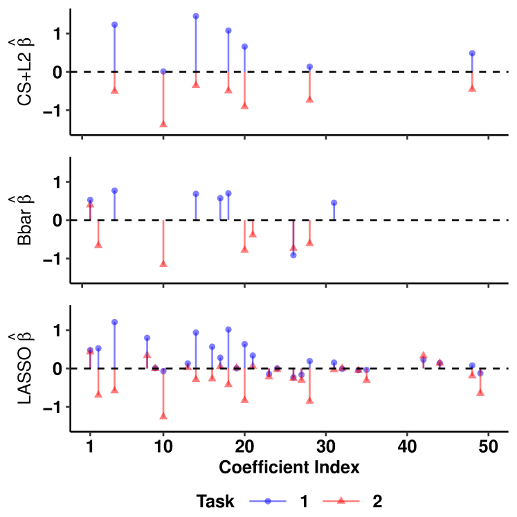
Figure 3: The Zbar+L2 method improves support recovery and coefficient estimate accuracy. The top left panel shows the true $\bm{\beta}$. Other panels show coefficient estimates. Color and symbol indicate task index.

5.2 Real Data Applications

We explore the performance of our methods in two multi-task biology settings to showcase different properties of the proposed estimators. First we explore performance in a chemometrics neuroscience application to demonstrate the method’s suitability to compression settings. This application includes a collection of datasets, where each dataset is treated as a separate task. Each task was collected with a different recording electrode. Exploratory analyses suggested the SHR methods were well suited to these data because regression coefficient estimates fit to each task differed substantially in both their support and values. In the second application, we explore a “multi-label” setting where the design matrix is fixed but the outcome differs across tasks (i.e., a multivariate outcome). Interpretability of model coefficients is of key importance in this application because the covariates are expression levels of genes in a network.

5.2.1 Neuroscience Application

Neuroscience Application Background:

Studying neurotransmitters (e.g., dopamine), that serve as chemical messengers between brain cells (neurons) is critical for developing treatments for neurological diseases. Recently, the application of Fast Scan Cyclic Voltammetry (FSCV) has been used to study neurotransmitter levels in humans (Kishida and others, 2016, 2011). The implementation of FSCV in humans relies on prediction methods to estimate neurotransmitter concentration based upon the raw electrical current measurements recorded by electrodes (a high dimensional time series signal). This vector of current measurements at a given time point can be used as covariates to model the concentration of a neurotransmitter. In vitro datasets are generated to serve as training sets because the true concentrations, the outcome, are known (i.e., the data are labelled). The trained models are then used to make predictions of neurochemical concentration in the brain. In practice, each in vitro dataset is generated on a different electrode, which we treat as a task here because signals of each electrode differ in the marginal distribution of the covariates and in the conditional distribution of the outcome given the covariates (Loewinger and others, 2022; Bang and others, 2020; Kishida and others, 2016; Moran and others, 2018). Given the high dimensional nature of the recordings, researchers typically apply regularized linear models (Kishida and others, 2016). Importantly, estimates from sparse linear models fit on each task separately (TS-SR) exhibit considerable heterogeneity in both the coefficient values and support as can be seen in Figure 4. For these reasons, we hypothesized that multi-task methods that employ regularizers that encourage models to share information through the $\bm{\beta}_{k}$ values (e.g., the Bbar method) would perform worse than methods that share information through the supports, $\bm{z}_{k}$ (i.e., the Zbar methods). We provide a more detailed description of this application in Supplement F.1.

We explored the performance of our methods at different values of $n_{k}$ and $p$. This is motivated by the fact that labs that use FSCV have reported fitting models with only a subset of the covariates (Montague and others, 2019) as the covariate values are on the same scale and units, and contain redundant information. This allows us to characterize the performance of our methods at different aspect ratios of $n_{k}/p$.

Neuroscience Application Modeling:

In order to assess out-of-sample prediction performance as a function of $n_{k}$ and $p$, we repeated the following 100 times. For each replicate, we randomly selected with uniform probability $K=4$ out of the total 15 datasets (tasks) to train models on. For each set of tasks, we split the datasets into training and testing sets and fit models on each task’s training data. We used the fit for task $k$, $\hat{\bm{\beta}}_{k}$, to make predictions on the test set of task $k$ and estimated performance as described above and in Supplemental Section D.2. Since our methods were developed for sparsity, we tuned the group Lasso hyperparameter to the best cross-validated value that produced a solution that had a cardinality no greater than the maximum value of $s$ in the tuning grid for the $\ell_{0}$ methods. If no cardinality constraints were imposed on the Lasso, cross-validation tended to select regularization hyperparameter values that resulted in solutions with large support sizes. As expected, these dense solutions tended to yield better prediction performance than the sparse solutions from the $\ell_{0}$ methods. We therefore constrained the Lasso and $\ell_{0}$ methods to provide equally sparse solutions. Indeed, the Ridge tended to exhibit the best prediction performance as it yielded the least sparse solutions of any methods explored. We provide more details about our modeling and tuning procedure in Supplemental Section F.2.

Neuroscience Application Results:

We first evaluated the hypothesis that sparse regression models fit separately to each task exhibited support heterogeneity. To characterize this observed pattern, we tuned and fit a TS-SR on four of the 15 available tasks (in vitro datasets) with sparsity $s=50$ and plotted the coefficient estimates in Figure 4. We only inspected one set of tasks to plot in order to avoid biases. The support of the estimates differed markedly between tasks and for some covariates, coefficient estimates were positive for some tasks and negative for others. The values of the nonzero coefficients varied so greatly across tasks that we had to use a log-transformation to visualize them all on the same scale. We also tuned and fit a Zbar+L2 method to visualize the impact of the SHR (Figure 4). The Zbar method increased the degree of support homogeneity, which we defined as $\binom{K}{2}^{-1}p^{-1}\sum_{j=1}^{p}\sum_{k=1}^{K}\sum_{l<k}\hat{z}_{k,j}\hat{z}_{l,j}$, (more details are provided in Supplemental Section D.2) by roughly 4.5 fold. We include a greater description of the methods as well as a figure that shows the support across the full vector of covariates in Supplement F.3.

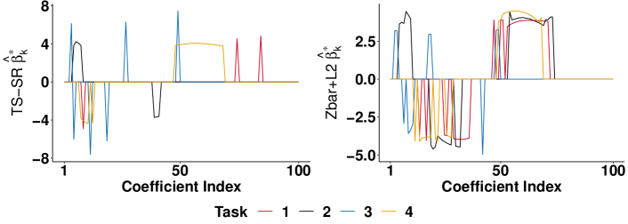
Figure 4: Coefficient estimates without [Left] and with [Right] SHR. To show the solutions on the same scale across tasks, we plot the nonzero elements of $\hat{\bm{\beta}}_{k}^{*}=sgn(\hat{\bm{\beta}}_{k})\odot\log(|\hat{\bm{\beta}}_{k}|)$.

Figure 5: Out-of-sample prediction performance (RMSE) averaged across random sets of tasks ($K=4$) for different $p$ (displayed on the x-axis) and $n_{k}$ (displayed on the panels).

We next study the out-of-sample prediction performance of our methods as a function of $n_{k}$ and $p$ averaged across tasks, as described in Supplemental Section D.2. We show boxplots in Figure 5. The Zbar+L2 method consistently outperformed the other $\ell_{0}$ methods tested. Interestingly, both methods that encourage models to borrow information directly through the $\bm{\beta}_{k}$ values, the Bbar and group Lasso, perform well when $p$ is low, but their performance degrades as $p$ increases. This is reminiscent of a related pattern we witnessed in simulations. In the simulation results displayed in Supplemental Figure E.2, we observed that the Bbar and group Lasso, performed comparably to the Zbar methods at higher SNRs, but their performance relative to other methods decreased as the SNR fell. Importantly, including a Zbar penalty alongside the Bbar penalty (i.e., Zbar+Bbar) lead to a far lower decrement in performance as a function of $p$ than models fit with the Bbar penalty alone. This suggests that including a penalty that encourages tasks to share information through the supports can improve prediction performance even when used alongside a penalty that encourages tasks to share information through the coefficient values. The common support $\ell_{0}$ methods performed worse than the benchmark TS-SR methods that allowed for support heterogeneity in every setting tested. The relative performance of the methods did not differ greatly across sample sizes.

5.2.2 Cancer Genomics Application

We next explore the performance of our method in a cancer biology application to highlight the method’s strength in high-dimensional genomics settings where interpretability is critical. This also serves as an important point of comparison because unlike the neuroscience application, one might expect common support methods to perform well in this application given that the tasks are defined by different gene expression levels from the same network of highly correlated genes. We build off of work (De Vito and others, 2021) focused on a multi-study dataset of breast cancer gene expression measurements. In cancer biology, the elucidation of regulatory gene network structure is critical for the characterization of the biology of disease subtypes and potentially the development of targeted therapeutics. As such, we sought to jointly predict the expression levels of a group of highly co-expressed genes based upon the expression levels of all other genes in the dataset. In view of the importance of the Estrogen Receptor (ESR1) in breast cancer development and therapy, we selected the expression levels of ESR1 and co-regulated genes FOXA1, TBC1D9, GATA3, MLPH, CA12, XBP1 and KRT18 to serve as the outcome for each task as these were found to be highly inter-connected in De Vito and others (2021). We selected the final set of genes before fitting any models to avoid biases. The dataset is comprised of data from 18 studies. In order to assess out-of-sample prediction performance, we implemented a hold-one-study-out testing procedure, whereby we iteratively fit models for each of the tasks on 17 of the datasets and tested prediction accuracy of those tasks jointly on the held-out study. To explore prediction performance as a function of $K$ and $p$, we ran 100 replicates of the following experiments: we randomly selected 1) $K$ of of the eight possible outcome variables to serve as tasks, 2) $p$ of the total covariates, and 3) one of the studies to serve as a held-out test set. For each replicate, we fit all models and compared performance. We considered all combinations of $K\in\{2,4,6\}$ and $p\in\{100,200,1000\}$. We tuned the model sparsity level across a grid that allowed for at most 50 nonzero coefficients, with local search. Other parameter tuning was conducted as described in Section 5.2.1. As the original dataset had over 10,000 covariates, we first reduced the dimension of the covariates to less than 2,000 through using only those covariates associated with coefficients selected in a group Lasso model fit to the full set of covariates. We then fit models on a set of covariates randomly selected from this smaller dataset.

As in the neuroscience application, the group Lasso often selected dense supports if the regularization hyperparameter was tuned based on prediction performance only. Consistent with this observation, methods like Ridge regression outperformed sparse methods. For fair comparisons, we therefore tuned the group Lasso under the constraint that the solution had to be as sparse as $\ell_{0}$ methods’ solutions.

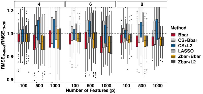
Figure 6: Hold-one-study-out prediction performance of $\ell_{0}$ methods averaged across tasks for different $K$. The performance (RMSE) is presented relative to the performance of task-specific sparse regressions.

We observed that the support heterogeneous methods consistently outperformed the common support methods, especially for higher $K$. However, unlike in the neuroscience application, the Bbar method performed comparably to the Zbar methods. Interestingly, the relative performance of the common support methods decreased as a function of $p$.

5.2.3 Application Comparison

The comparison between the Zbar and the Bbar methods in these two applications sheds light on when a continuous penalty that shrinks the $\bm{\beta}_{k}$ values together can perform as well as a discrete penalty that shrinks the $\bm{\beta}_{k}$ supports together. While the two datasets differ in many ways, inspection of simple measures of the distribution of the $\hat{{\beta}}_{k,j}$ across tasks, $k$, reveal important insights. For each application, we fit task-specific Ridge regressions and compared rug plots of the $\hat{\beta}_{k,j}$ across tasks for the 10 most “important” covariates (Figure 7). Specifically, we selected the 10 $j$’s associated with the greatest average magnitude of coefficient estimates ($\frac{1}{K}\sum_{k=1}^{K}|\hat{\beta}_{k,j}|$). Importantly, the estimates in the cancer plots are all positive, have similar values and are relatively far from zero, potentially reflecting low heterogeneity in the coefficient signs, values and supports. The Bbar penalty might therefore be expected to perform well in this application. The FSCV estimates, on the other hand, exhibit considerable heterogeneity in coefficient values and signs. Moreover, for some covariates, a subset of the task estimates have large magnitudes while the other task estimates are close to 0, potentially reflecting support heterogeneity. In cases like these, a penalty that encourages information sharing through the coefficient supports may be preferable to penalties that share information by shrinking the $\bm{\beta}_{k}$ values together. These patterns may partially explain why the Zbar+L2 method strongly outperformed the Bbar method in the neuroscience application but performed similarly to the Bbar method in the cancer genomics application.

Interestingly, the FSCV coefficient estimates also tended to fall into clusters of similar patterns (e.g., Coefficients 1, 5, and 10 comprise one cluster) on the rug plot. This may be because the covariates in the FSCV dataset exhibit much of the structure characteristic of functional covariates such as a natural ordering and similar levels of correlation with the outcome across adjacent covariates (see Loewinger and others (2022)). More extensive rug plots in Supplemental Section G confirm that the patterns described above are representative across a large set of covariates.

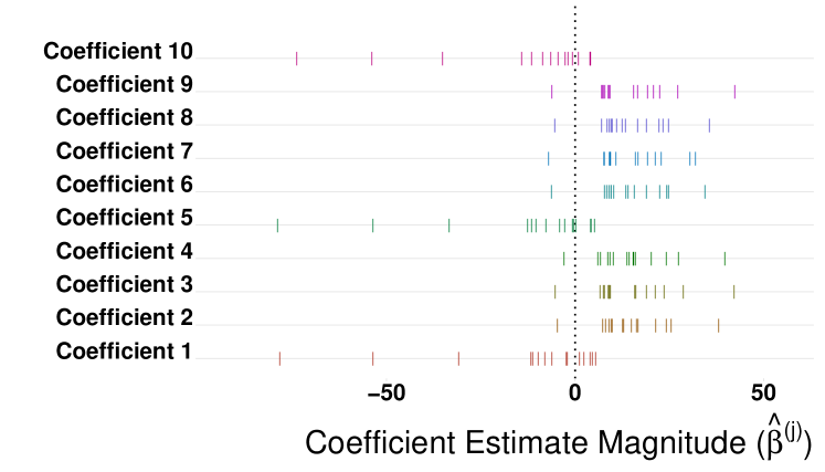
Figure 7: Rug plots displaying $\hat{\beta}_{k,j}$ for the 10 $j$’s with the greatest average magnitude across the $K$ task-specific Ridge regressions ($\frac{1}{K}\sum_{k=1}^{K}|\hat{\beta}_{k,j}|$). For Coefficient $j$, each mark on the horizontal line is one of $K$ task-specific empirical estimates of the $\hat{\bm{\beta}}_{k,j}$. [Left] FSCV. [Right] Breast Cancer

.

6 Discussion

We propose a class of estimators that penalize the heterogeneity across tasks in the support vectors $\bm{z}_{k}$. These methods allow for information to be shared directly through the support of regression parameters without relying on methods that shrink coefficient values together, an approach that can perform poorly when the distribution of coefficient values differ substantially between tasks. Our theoretical analysis shows that the Zbar penalty shrinks the supports together across tasks, improves support recovery accuracy when the true regression coefficients have (near) common support, and maintains statistically optimal prediction performance. We developed algorithms based on block CD and local search to obtain high-quality solutions to our estimator. Our numerical experiments on synthetic and real data show the usefulness of our method. Taken together, the present work is an important methodological contribution to the multi-task learning literature.

7 Software and Reproducibility

Code and instructions to reproduce analyses, figures and tables are available at: https://github.com/gloewing/sMTL. This contains code to tune and fit penalized linear regression problems with all the methods assessed here. Block CD and local search algorithms are coded in Julia and are called from R where simulations and data analyses are implemented. We will release the R package, sMTL, that implements all sparse regression methods implemented here for multi-task learning, domain generalization, multi-label learning as well as standard sparse regression for single dataset/task settings.

Appendix A Mixed-Integer Program Formulations

We provide a big-M notation formulation of the problems (2) and (3) that can be solved to optimality with solvers such as Gurobi, MOSEK or CPLEX that employ, for example, branch and bound algorithms. Below $M$ is a large positive constant that is selected before the optimization (e.g., see formulations to the related best subset selection problem in (Bertsimas and others, 2016)). If $M$ is sufficiently large, the choice will not affect the solution, although it can impact the speed of convergence. Problems (A.1) and (A.2) below present equivalent MIP reformulations for problems (2) and (3), respectively.

$$\underset{\bm{z},~{}\mathbb{B},\bar{\bm{\beta}}}{\mbox{min }}\sum_{k=1}^{K}\frac{1}{n_{k}}\left\lVert\mathbf{y}_{k}-\mathbb{X}_{k}\bm{\beta}_{k}\right\rVert_{2}^{2}+\lambda\sum_{k=1}^{K}\left\lVert\bm{\beta}_{k}-\bar{{\bm{\beta}}}\right\rVert_{2}^{2}$$ (A.1)

$$\mbox{subject to: }~{}z_{j}\in\{0,1\}~{}~{}\forall~{}j\in[p]$$

$$~{}~{}~{}~{}~{}~{}~{}~{}~{}~{}~{}~{}~{}~{}~{}~{}-Mz_{j}\leq\beta_{k,j}\leq Mz_{j}~{}~{}\forall~{}k\in[K],~{}\forall~{}j\in[p]$$

$$~{}~{}~{}~{}~{}~{}~{}~{}~{}~{}~{}~{}~{}~{}~{}~{}~{}~{}\sum_{j=1}^{p}z_{j}\leq s.$$

$$\underset{\mathbb{Z},~{}\mathbb{B},\bar{\bm{\beta}},\bar{\bm{z}}}{\mbox{min }}\sum_{k=1}^{K}\frac{1}{n_{k}}\left\lVert\mathbf{y}_{k}-\mathbb{X}_{k}\bm{\beta}_{k}\right\rVert_{2}^{2}+\lambda\sum_{k=1}^{K}\left\lVert\bm{\beta}_{k}-\bar{{\bm{\beta}}}\right\rVert_{2}^{2}+\delta\sum_{k=1}^{K}\left\lVert\bm{z}_{k}-\bar{\bm{z}}\right\rVert_{2}^{2}$$ (A.2)

$$\mbox{subject to: }~{}z_{k,j}\in\{0,1\}~{}~{}\forall~{}j\in[p]$$

$$~{}~{}~{}~{}~{}~{}~{}~{}~{}~{}~{}~{}~{}~{}~{}~{}-Mz_{k,j}\leq\beta_{k,j}\leq Mz_{k,j}~{}~{}\forall~{}k\in[K],~{}\forall~{}j\in[p],$$

$$~{}~{}~{}~{}~{}~{}~{}~{}~{}~{}~{}~{}~{}~{}~{}~{}~{}~{}\sum_{j=1}^{p}z_{k,j}\leq s~{}~{}\forall~{}k\in[K].$$

Appendix B Details from Algorithm Implementation

B.1 Block CD Algorithm

In this section, we discuss how problem (9) can be solved efficiently. Suppose $k\in[K]$ is given and fixed. The goal is to find the optimal values of $\bm{\beta}_{k},\bm{z}_{k}$. As $\bm{z}_{k}$ is a binary vector, for $j\in[p]$ we consider two cases $z_{k,j}=0,1$. If $z_{k,j}=1$, the optimal value of $\beta_{k,j}$ is given as

$$\beta_{k,j}=b_{k,j}:=\beta_{k,j}^{+}-\frac{1}{L_{k}}\frac{\partial g_{k}(\bm{\beta}_{k}^{+},\bar{\bm{\beta}})}{\partial\beta_{k,j}}.$$

Moreover, $(z_{k,j}-\bar{z}_{j})^{2}=(1-\bar{z}_{j})^{2}$. If $z_{k,j}=0$, then we have $\beta_{k,j}=0$ and $(z_{k,j}-\bar{z}_{j})^{2}=\bar{z}_{j}^{2}$. Hence, the difference in the contribution of term $j$ in the objective of (9) for $z_{k,j}=1,0$ is

$$\Delta_{k,j}=(1-\bar{z}_{j})^{2}-\left(\frac{L_{k}}{2}b_{k,j}^{2}+\bar{z}_{j}^{2}\right).$$

If $\Delta_{k,j}\geq 0$, setting $z_{k,j}=0$ leads to a lower objective and therefore for any such $j$, the optimal values are given as $\beta_{k,j}=z_{k,j}=0$. For any other $j$, setting $z_{k,j}=1$ results in a lower objective, however, at most $s$ of values of $z_{k,j}$ can be set to one to ensure feasibility. As a result, we select at most $s$ values of $j$ that lead to smallest (most negative) value of $\Delta_{k,j}$.

B.2 Active Sets

To further speed-up the convergence of our algorithm, we implement an active set version of the block CD algorithm. We start by an initial active set $\mathcal{I}_{\text{active}}$. Then, we run the block CD algorithm on problem (3) with the additional constraint

$$\beta_{k,j}=0~{}~{}\forall k\in[K],j\notin\mathcal{I}_{\text{active}}.$$

Under this constraint, the dimension of the problem is effectively reduced to $|\mathcal{I}_{\text{active}}|$, instead of $p$, which leads to faster convergence if $|\mathcal{I}_{\text{active}}|\ll p$. After the solution to the restricted problem is found, we run an iteration of block CD on the original problem (problem (3)) with $p$ features. If this iteration does not change the solution, the current solution to the restricted problem is also a solution to the original problem. Otherwise, we update the active set as

$$\mathcal{I}_{\text{active}}\leftarrow\mathcal{I}_{\text{active}}\cup\{j:\exists k\in[K]:\beta_{k,j}\neq 0\}.$$

B.3 Local Search Method

Suppose $k_{0}\in[K]$ is fixed. In Proposition B.1 below, we give a closed form solution for the inner optimization in problem (11) (i.e., the value of $b$ for given $j_{1},j_{2}$).

Proposition B.1.

Fix $k_{0},j_{1},j_{2}$ in problem (11). Let $\tilde{b}$ be the optimal solution to the inner problem in Problem (11). Moreover, let

$$\mathbf{r} =\mathbf{y}_{k_{0}}-\mathbb{X}_{k_{0}}\tilde{\bm{\beta}}_{k_{0}}$$ (B.1)

$$p_{1} =\frac{\|\mathbf{x}_{k_{0},j_{2}}\|_{2}^{2}}{n_{k_{0}}}+\alpha+\lambda\frac{K^{2}-K}{K^{2}}$$

$$p_{2} =-\frac{2}{n_{k_{0}}}\mathbf{r}^{T}\mathbf{x}_{k_{0},j_{2}}-\frac{2}{n_{k_{0}}}\mathbf{x}_{k_{0},j_{2}}^{T}\mathbf{x}_{k_{0},j_{1}}\tilde{\beta}_{k_{0},j_{1}}-\frac{2\lambda}{K}\sum_{k=1}^{K}\tilde{\beta}_{k,j_{2}}$$

$$p_{3} =\frac{\|\mathbf{x}_{k_{0},j_{1}}\|_{2}^{2}}{n_{k_{0}}}\tilde{\beta}_{k_{0},j_{1}}^{2}+\frac{1}{n_{k_{0}}}\mathbf{r}^{T}\mathbf{x}_{k_{0},j_{1}}\tilde{\beta}_{k_{0},j_{1}}.$$

Then,

1. One has

   $$\tilde{b}=-\frac{p_{2}}{2p_{1}}.$$

2. Moreover,

   $$g(\tilde{\mathbb{B}}-\tilde{\beta}_{k_{0},j_{1}}\bm{E}_{k_{0},j_{1}}+\tilde{b}\bm{E}_{k_{0},j_{2}})-g(\tilde{\mathbb{B}})=p_{3}-\frac{p_{2}^{2}}{4p_{1}}\\ -\lambda\left[\sum_{k=1}^{K}\left(\tilde{\beta}_{k,j_{1}}-\frac{\sum_{k=1}^{K}\tilde{\beta}_{k,j_{1}}}{K}\right)^{2}\right]+\lambda\left[\sum_{k:k\neq k_{0}}^{K}\left(\tilde{\beta}_{k,j_{1}}-\frac{\sum_{k:k\neq k_{0}}\tilde{\beta}_{k,j_{1}}}{K}\right)^{2}\right]+\lambda\left(\frac{\sum_{k:k\neq k_{0}}\tilde{\beta}_{k,j_{1}}}{K}\right)^{2}$$

   and

   $$h(\tilde{\bm{Z}}-\bm{E}_{k_{0},j_{1}}+\bm{E}_{k_{0},j_{2}})-h(\tilde{\bm{Z}})=\\ -\delta\left[\sum_{k=1}^{K}\left(\tilde{z}_{k,j_{1}}-\frac{\sum_{k=1}^{K}\tilde{z}_{k,j_{1}}}{K}\right)^{2}\right]+\delta\left[\sum_{k:k\neq k_{0}}^{K}\left(\tilde{z}_{k,j_{1}}-\frac{\sum_{k:k\neq k_{0}}\tilde{z}_{k,j_{1}}}{K}\right)^{2}\right]+\delta\left(\frac{\sum_{k:k\neq k_{0}}\tilde{z}_{k,j_{1}}}{K}\right)^{2}.$$

Proposition B.1 shows that the inner optimization in problem (11), and therefore the entire mathematical program 11, can be solved efficiently via a closed form solution. In our implementation, we perform the calculations described in Proposition B.1 in matrix form. As a result, we can identify the optimal swap for each $k$ without any for loops over $j_{1},j_{2}$. Our numerical experiments confirm the benefits of local search in practice.

Appendix C Proofs of Main Results

C.1 Proof of Theorem 1

The proof of this theorem is based on the following technical lemma.

Lemma C.1.

Suppose $\bm{X}\in\mathbb{R}^{n\times p}$ is independent of $\bm{\epsilon}\sim\mathcal{N}(0,\sigma^{2}\bm{I}_{n})$. Let

$$\mathcal{E}(\bm{X},\bm{\epsilon})=\left\{\sup_{\begin{subarray}{c}\bm{v}\in\mathbb{R}^{p}\\ \|\bm{v}\|_{0}\leq 2s\end{subarray}}\left|\bm{\epsilon}^{T}\frac{\bm{Xv}}{\|\bm{Xv}\|_{2}}\right|\leq c_{1}\sigma\sqrt{s\log(p/s)}\right\}$$ (C.1)

for some absolute constant $c_{1}>0$. Then

$${\rm I}\kern-1.79993pt{\rm P}(\mathcal{E}(\bm{X},\bm{\epsilon}))\geq 1-\exp(-10s\log(p/s)).$$

Proof.

For any $S\subseteq[p]$, let $\bm{X}_{S}\in\mathbb{R}^{n\times|S|}$ be the submatrix of $\bm{X}$ with columns indexed by $S$. Moreover, let $\bm{\Phi}_{S}\in\mathbb{R}^{p\times|S|}$ be an orthonormal basis for the column span of $\bm{X}_{S}$. One has

$${\rm I}\kern-1.79993pt{\rm P}\left(\left.\sup_{\begin{subarray}{c}\bm{v}\in\mathbb{R}^{p}\\ \|\bm{v}\|_{0}\leq 2s\end{subarray}}\left|\bm{\epsilon}^{T}\frac{\bm{Xv}}{\|\bm{Xv}\|_{2}}\right|>t\right|\bm{X}\right) ={\rm I}\kern-1.79993pt{\rm P}\left(\left.\max_{\begin{subarray}{c}S\subseteq[p]\\ |S|=2s\end{subarray}}\sup_{\begin{subarray}{c}\bm{v}\in\mathbb{R}^{p}\\ S(\bm{v})=S\end{subarray}}\left|\bm{\epsilon}^{T}\frac{\bm{Xv}}{\|\bm{Xv}\|_{2}}\right|>t\right|\bm{X}\right)$$

$$\stackrel{{\scriptstyle(a)}}{{=}}{\rm I}\kern-1.79993pt{\rm P}\left(\left.\max_{\begin{subarray}{c}S\subseteq[p]\\ |S|=2s\end{subarray}}\sup_{\begin{subarray}{c}\bm{v}\in\mathbb{R}^{|S|}\\ \|\bm{v}\|_{2}=1\end{subarray}}(\bm{\Phi}_{S}^{T}\bm{\epsilon})^{T}\bm{v}>t\right|\bm{X}\right)$$

$$\stackrel{{\scriptstyle(b)}}{{\leq}}{p\choose 2s}{\rm I}\kern-1.79993pt{\rm P}\left(\left.\sup_{\begin{subarray}{c}\bm{v}\in\mathbb{R}^{|S|}\\ \|\bm{v}\|_{2}=1\end{subarray}}(\bm{\Phi}_{S}^{T}\bm{\epsilon})^{T}\bm{v}>t\right|\bm{X}\right)$$

$$\stackrel{{\scriptstyle(c)}}{{\leq}}{p\choose 2s}\exp\left(-\frac{t^{2}}{8\sigma^{2}}+2s\log 5\right)$$

$$\stackrel{{\scriptstyle(d)}}{{\leq}}\left(\frac{ep}{2s}\right)^{2s}\exp\left(-\frac{t^{2}}{8\sigma^{2}}+2s\log 5\right)$$

$$\leq\exp\left(-\frac{t^{2}}{8\sigma^{2}}+2s\log 5+2s\log(ep/2s)\right)$$

where $(a)$ is due to the definition of $\bm{\Phi}_{S}$, $(b)$ is due to union bound, $(c)$ is true as by independence of $\bm{X}$ and $\bm{\epsilon}$, we have $\bm{\Phi}_{S}^{T}\bm{\epsilon}|\bm{X}\sim\mathcal{N}(\bm{0},\sigma^{2}\bm{I}_{2s})$ and Theorem 1.19 of Rigollet and Hütter (2015) and $(d)$ is by the inequality ${p\choose 2s}\leq(ep/2s)^{2s}$. Take $t^{2}=64\sigma^{2}c_{1}s\log(p/s)$ and $c_{1}$ large enough to have that $8c_{1}s\log(p/s)-2s\log 5-2s\log(ep/2s)>10s\log(p/s)$. As a result,

$${\rm I}\kern-1.79993pt{\rm P}\left(\left.\mathcal{E}(\bm{X},\bm{\epsilon})\right|\bm{X}\right)\geq 1-\exp(-10s\log(p/s)).$$ (C.2)

Finally, note that

$${\rm I}\kern-1.79993pt{\rm P}(\mathcal{E}(\bm{X},\bm{\epsilon}))=\int_{\bm{X}}{\rm I}\kern-1.79993pt{\rm P}\left(\left.\mathcal{E}(\bm{X},\bm{\epsilon})\right|\bm{X}\right)d{\rm I}\kern-1.79993pt{\rm P}_{\bm{X}}\geq\int_{\bm{X}}(1-\exp(-10s\log(p/s)))d{\rm I}\kern-1.79993pt{\rm P}_{\bm{X}}=1-\exp(-10s\log(p/s)).$$

∎

Proof of Theorem 1.

The proof of this theorem is based on the intersection of events $\mathcal{E}(\mathbb{X}_{1},\bm{\epsilon}_{1}),\cdots,\mathcal{E}(\mathbb{X}_{K},\bm{\epsilon}_{K})$ which by Lemma C.1 and union bound happens with probability at least

$$1-K\exp(-10s\log(p/s)).$$ (C.3)

To lighten the notation, let

$$h(\bm{z}_{1},\cdots,\bm{z}_{K})=\delta\sum_{k=1}^{K}\|\bm{z}_{k}-\bar{\bm{z}}\|_{2}^{2}$$

with $\bar{\bm{z}}=\sum_{k=1}^{K}\bm{z}_{k}/K$. By optimality of $\hat{\bm{\beta}}_{k},\hat{\bm{z}}_{k}$ and feasibility of $\bm{\beta}_{k}^{*},\bm{z}_{k}^{*}$ for problem (3), we have:

$$\sum_{k=1}^{K}\frac{1}{n_{k}}\|\mathbf{y}_{k}-\mathbb{X}_{k}\hat{\bm{\beta}}_{k}\|_{2}^{2}+h(\hat{\bm{z}}_{1},\cdots,\hat{\bm{z}}_{K})\leq\sum_{k=1}^{K}\frac{1}{n_{k}}\|\mathbf{y}_{k}-\mathbb{X}_{k}{\bm{\beta}}^{*}_{k}\|_{2}^{2}+h(\bm{z}_{1}^{*},\cdots,\bm{z}_{K}^{*})$$

$$\stackrel{{\scriptstyle(a)}}{{\Rightarrow}} \sum_{k=1}^{K}\frac{1}{n_{k}}\|\mathbb{X}_{k}\bm{\beta}_{k}^{*}+\bm{r}_{k}+\bm{\epsilon}_{k}-\mathbb{X}_{k}\hat{\bm{\beta}}_{k}\|_{2}^{2}+h(\hat{\bm{z}}_{1},\cdots,\hat{\bm{z}}_{K})\leq\sum_{k=1}^{K}\frac{1}{n_{k}}\|\bm{r}_{k}+\bm{\epsilon}_{k}\|_{2}^{2}+h(\bm{z}_{1}^{*},\cdots,\bm{z}_{K}^{*})$$

$$\Rightarrow \sum_{k=1}^{K}\frac{1}{n_{k}}\|\mathbb{X}_{k}(\bm{\beta}_{k}^{*}-\hat{\bm{\beta}}_{k})\|_{2}^{2}+h(\hat{\bm{z}}_{1},\cdots,\hat{\bm{z}}_{K})\leq\sum_{k=1}^{K}\frac{-2}{n_{k}}(\bm{\epsilon}_{k}+\bm{r}_{k})^{T}\mathbb{X}_{k}(\bm{\beta}_{k}^{*}-\hat{\bm{\beta}}_{k})+h(\bm{z}_{1}^{*},\cdots,\bm{z}_{K}^{*})$$

$$\Rightarrow \sum_{k=1}^{K}\frac{1}{n_{k}}\|\mathbb{X}_{k}(\bm{\beta}_{k}^{*}-\hat{\bm{\beta}}_{k})\|_{2}^{2}+h(\hat{\bm{z}}_{1},\cdots,\hat{\bm{z}}_{K})\leq\sum_{k=1}^{K}\frac{-2}{n_{k}}(\bm{\epsilon}_{k}+\bm{r}_{k})^{T}\frac{\mathbb{X}_{k}(\bm{\beta}_{k}^{*}-\hat{\bm{\beta}}_{k})}{\|\mathbb{X}_{k}(\bm{\beta}_{k}^{*}-\hat{\bm{\beta}}_{k})\|_{2}}\|\mathbb{X}_{k}(\bm{\beta}_{k}^{*}-\hat{\bm{\beta}}_{k})\|_{2}+h(\bm{z}_{1}^{*},\cdots,\bm{z}_{K}^{*})$$

$$\stackrel{{\scriptstyle(b)}}{{\Rightarrow}} \sum_{k=1}^{K}\frac{1}{2n_{k}}\|\mathbb{X}_{k}(\bm{\beta}_{k}^{*}-\hat{\bm{\beta}}_{k})\|_{2}^{2}+h(\hat{\bm{z}}_{1},\cdots,\hat{\bm{z}}_{K})\leq\sum_{k=1}^{K}\frac{2}{n_{k}}\left((\bm{\epsilon}_{k}+\bm{r}_{k})^{T}\frac{\mathbb{X}_{k}(\bm{\beta}_{k}^{*}-\hat{\bm{\beta}}_{k})}{\|\mathbb{X}_{k}(\bm{\beta}_{k}^{*}-\hat{\bm{\beta}}_{k})\|_{2}}\right)^{2}+h(\bm{z}_{1}^{*},\cdots,\bm{z}_{K}^{*}),$$ (C.4)

where $(a)$ is achieved by substituting $\mathbf{y}_{k}=\mathbb{X}_{k}\bm{\beta}_{k}^{*}+\bm{\epsilon}_{k}+\bm{r}_{k}$ from the oracle, and $(b)$ is a result of the inequality $-2ab\leq 2a^{2}+b^{2}/2$. Next, note that $\bm{\beta}_{k}^{*}-\hat{\bm{\beta}}_{k}$ has at most $2s$ nonzero coordinates. As a result, from event $\mathcal{E}(\mathbb{X}_{k},\bm{\epsilon}_{k})$ write

$$\frac{1}{n_{k}}\left(\bm{\epsilon}_{k}^{T}\frac{\mathbb{X}_{k}(\bm{\beta}_{k}^{*}-\hat{\bm{\beta}}_{k})}{\|\mathbb{X}_{k}(\bm{\beta}_{k}^{*}-\hat{\bm{\beta}}_{k})\|_{2}}\right)^{2}\lesssim\frac{\sigma_{k}^{2}s\log(p/s)}{n_{k}}.$$ (C.5)

Moreover,

$$\frac{1}{n_{k}}\left((\bm{\epsilon}_{k}+\bm{r}_{k})^{T}\frac{\mathbb{X}_{k}(\bm{\beta}_{k}^{*}-\hat{\bm{\beta}}_{k})}{\|\mathbb{X}_{k}(\bm{\beta}_{k}^{*}-\hat{\bm{\beta}}_{k})\|_{2}}\right)^{2} \lesssim\frac{1}{n_{k}}\left(\bm{r}_{k}^{T}\frac{\mathbb{X}_{k}(\bm{\beta}_{k}^{*}-\hat{\bm{\beta}}_{k})}{\|\mathbb{X}_{k}(\bm{\beta}_{k}^{*}-\hat{\bm{\beta}}_{k})\|_{2}}\right)^{2}+\frac{1}{n_{k}}\left(\bm{\epsilon}_{k}^{T}\frac{\mathbb{X}_{k}(\bm{\beta}_{k}^{*}-\hat{\bm{\beta}}_{k})}{\|\mathbb{X}_{k}(\bm{\beta}_{k}^{*}-\hat{\bm{\beta}}_{k})\|_{2}}\right)^{2}$$

$$\lesssim\frac{1}{n_{k}}\|\bm{r}_{k}\|_{2}^{2}+\frac{1}{n_{k}}\left(\bm{\epsilon}_{k}^{T}\frac{\mathbb{X}_{k}(\bm{\beta}_{k}^{*}-\hat{\bm{\beta}}_{k})}{\|\mathbb{X}_{k}(\bm{\beta}_{k}^{*}-\hat{\bm{\beta}}_{k})\|_{2}}\right)^{2}.$$ (C.6)

Consequently, from (C.4) and (C.5) we have

$$\sum_{k=1}^{K}\frac{1}{n_{k}}\|\mathbb{X}_{k}(\bm{\beta}_{k}^{*}-\hat{\bm{\beta}}_{k})\|_{2}^{2}+h(\hat{\bm{z}}_{1},\cdots,\hat{\bm{z}}_{K})\lesssim\sum_{k=1}^{K}\frac{\sigma_{k}^{2}s\log(p/s)}{n_{k}}+h(\bm{z}_{1}^{*},\cdots,\bm{z}_{K}^{*})+\sum_{k=1}^{K}\frac{1}{n_{k}}\|\bm{r}_{k}\|_{2}^{2}.$$ (C.7)

∎

C.2 Proof of Corollary 1

The proof of this corollary is based on the following lemma.

Lemma C.2.

Suppose $\bm{z}_{1}\cdots,\bm{z}_{K}\in\{0,1\}^{p}$. Then,

$$\sum_{k=1}^{K}\|\bm{z}_{k}-\bar{\bm{z}}\|_{2}^{2}\geq\frac{|S_{\text{all}}\setminus S_{\text{common}}|}{K}$$

where $\bar{\bm{z}}=\sum_{k=1}^{K}\bm{z}_{k}/K$, $S_{\text{all}}=S_{\text{all}}(\bm{z}_{1},\cdots,\bm{z}_{K})$ and $S_{\text{common}}=S_{\text{common}}(\bm{z}_{1},\cdots,\bm{z}_{K})$.

Proof.

For $j\in S_{\text{common}}$ or $j\notin S_{\text{all}}$,

$$\sum_{k=1}^{K}(z_{k,j}-\bar{z}_{j})^{2}=0.$$

Suppose $j\in S_{\text{all}}\setminus S_{\text{common}}$. Then, there exist $k_{1},k_{2}\in[K]$ such that $z_{k_{1},j}=1$ and $z_{k_{2},j}=0$, implying $1/K\leq\bar{z}_{j}\leq(K-1)/K$. As a result, for $k_{0}\in[K]$ if $z_{k_{0},j}=0$,

$$(z_{k_{0},j}-\bar{z}_{j})^{2}=\bar{z}_{j}^{2}\geq\frac{1}{K^{2}}$$

and if $z_{k_{0},j}=1$,

$$(z_{k_{0},j}-\bar{z}_{j})^{2}=(1-\bar{z}_{j})^{2}\geq(1-(K-1)/K)^{2}\geq\frac{1}{K^{2}}.$$

Consequently,

$$\sum_{k=1}^{K}\|\bm{z}_{k}-\bar{\bm{z}}\|_{2}^{2}\geq\sum_{j\in S_{\text{all}}\setminus S_{\text{common}}}\sum_{k=1}^{K}(z_{k,j}-\bar{z}_{j})^{2}\geq\sum_{j\in S_{\text{all}}\setminus S_{\text{common}}}\sum_{k=1}^{K}\frac{1}{K^{2}}=\frac{|S_{\text{all}}\setminus S_{\text{common}}|}{K}.$$ (C.8)

∎

Proof of Corollary 1.

This proof is on the probability event considered in Theorem 1. Note that as $\bm{z}_{1}^{*}=\cdots=\bm{z}_{K}$, we have that $h(\bm{z}_{1}^{*},\cdots,\bm{z}_{K}^{*})=0$. The prediction error part of the corollary follows from this fact and Theorem 1. Let $\hat{S}_{\text{all}}=S_{\text{all}}(\hat{\bm{z}}_{1},\cdots,\hat{\bm{z}}_{K})$ and $\hat{S}_{\text{common}}=S_{\text{common}}(\hat{\bm{z}}_{1},\cdots,\hat{\bm{z}}_{K})$. Next,

$$\delta\frac{|\hat{S}_{\text{all}}\setminus\hat{S}_{\text{common}}|}{K} \stackrel{{\scriptstyle(a)}}{{\leq}}h(\hat{\bm{z}}_{1},\cdots,\hat{\bm{z}}_{K})$$

$$\leq\sum_{k=1}^{K}\frac{1}{n_{k}}\|\mathbb{X}_{k}(\bm{\beta}_{k}^{*}-\hat{\bm{\beta}}_{k})\|_{2}^{2}+h(\hat{\bm{z}}_{1},\cdots,\hat{\bm{z}}_{K})$$

$$\stackrel{{\scriptstyle(b)}}{{\lesssim}}\sum_{k=1}^{K}\frac{\sigma_{k}^{2}s\log(p/s)}{n_{k}}+\sum_{k=1}^{K}\frac{1}{n_{k}}\|\bm{r}_{k}\|_{2}^{2}$$ (C.9)

where $(a)$ is due to Lemma C.2 and $(b)$ is due to Theorem 1. In particular, if $\delta\gtrsim K\sum_{k=1}^{K}{([\sigma_{k}^{2}s\log(p/s)+\|\bm{r}_{k}\|_{2}^{2}]/n_{k})}$ is sufficiently large,

$$|\hat{S}_{\text{all}}\setminus\hat{S}_{\text{common}}|\lesssim\frac{K}{\delta}\sum_{k=1}^{K}\left[\frac{\sigma_{k}^{2}s\log(p/s)}{n_{k}}+\frac{1}{n_{k}}\|\bm{r}_{k}\|_{2}^{2}\right]\leq c^{*}$$ (C.10)

for some $c^{*}\in[0,1)$ and as $|\hat{S}_{\text{all}}\setminus\hat{S}_{\text{common}}|\in\mathbb{Z}_{\geq 0}$, we have that $|\hat{S}_{\text{all}}\setminus\hat{S}_{\text{common}}|=0$. ∎

C.3 Proof of Corollary 2

Lemma C.3.

Suppose $\bm{z}_{1}\cdots,\bm{z}_{K}\in\{0,1\}^{p}$ are regular. Then,

$$\sum_{k=1}^{K}\|\bm{z}_{k}-\bar{\bm{z}}\|_{2}^{2}=|S_{\text{all}}\setminus S_{\text{common}}|\frac{K^{2}-K}{K^{2}}$$

where $\bar{\bm{z}}=\sum_{k=1}^{K}\bm{z}_{k}/K$, $S_{\text{all}}=S_{\text{all}}(\bm{z}_{1},\cdots,\bm{z}_{K})$ and $S_{\text{common}}=S_{\text{common}}(\bm{z}_{1},\cdots,\bm{z}_{K})$.

Proof.

For $j\in S_{\text{common}}$ or $j\notin S_{\text{all}}$,

$$\sum_{k=1}^{K}(z_{k,j}-\bar{z}_{j})^{2}=0.$$

Suppose $j\in S_{\text{all}}\setminus S_{\text{common}}$ and $k_{0}\in[K]$ is such that $z_{k_{0},j}=1$. Then, $\bar{z}_{j}=1/K$ and

$$\sum_{k=1}^{K}(z_{k,j}-\bar{z}_{j})^{2}=\sum_{k=1}^{K}(z_{k,j}-1/K)^{2}=\frac{K-1}{K^{2}}+\frac{(K-1)^{2}}{K^{2}}=\frac{K^{2}-K}{K^{2}}.$$ (C.11)

As a result,

$$\sum_{k=1}^{K}\|\bm{z}_{k}-\bar{\bm{z}}\|_{2}^{2}=\sum_{j\in S_{\text{all}}\setminus S_{\text{common}}}\sum_{k=1}^{K}(z_{k,j}-\bar{z}_{j})^{2}=|S_{\text{all}}\setminus S_{\text{common}}|\frac{K^{2}-K}{K^{2}}.$$ (C.12)

∎

Proof of Corollary 2.

In this proof, we assume $\delta$ is taken as

$$\delta=c_{\delta}\frac{K}{K-1}\frac{1}{|S^{*}_{\text{all}}\setminus S^{*}_{\text{common}}|}\sum_{k=1}^{K}\left\{\frac{\sigma_{k}^{2}s\log(p/s)}{n_{k}}+\frac{1}{n_{k}}\|\bm{r}_{k}\|_{2}^{2}\right\}$$ (C.13)

where $c_{\delta}$ is an absolute constant.

This proof is on the probability event considered in Theorem 1. Let $\hat{S}_{\text{all}}=S_{\text{all}}(\hat{\bm{z}}_{1},\cdots,\hat{\bm{z}}_{K})$ and $\hat{S}_{\text{common}}=S_{\text{common}}(\hat{\bm{z}}_{1},\cdots,\hat{\bm{z}}_{K})$. One has

$$\sum_{k=1}^{K}\frac{1}{n_{k}}\|\mathbb{X}_{k}(\bm{\beta}_{k}^{*}-\hat{\bm{\beta}}_{k})\|_{2}^{2}+\delta\frac{|\hat{S}_{\text{all}}\setminus\hat{S}_{\text{common}}|}{K} \stackrel{{\scriptstyle(a)}}{{\leq}}\sum_{k=1}^{K}\frac{1}{n_{k}}\|\mathbb{X}_{k}(\bm{\beta}_{k}^{*}-\hat{\bm{\beta}}_{k})\|_{2}^{2}+h(\hat{\bm{z}}_{1},\cdots,\hat{\bm{z}}_{K})$$

$$\stackrel{{\scriptstyle(b)}}{{\lesssim}}\sum_{k=1}^{K}\left\{\frac{\sigma_{k}^{2}s\log(p/s)}{n_{k}}+\frac{1}{n_{k}}\|\bm{r}_{k}\|_{2}^{2}\right\}+h(\bm{z}_{1}^{*},\cdots,\bm{z}_{K}^{*})$$

$$\stackrel{{\scriptstyle(c)}}{{\lesssim}}\sum_{k=1}^{K}\left\{\frac{\sigma_{k}^{2}s\log(p/s)}{n_{k}}+\frac{1}{n_{k}}\|\bm{r}_{k}\|_{2}^{2}\right\}+\delta\frac{K^{2}-K}{K^{2}}|S^{*}_{\text{all}}\setminus S^{*}_{\text{common}}|$$

$$\stackrel{{\scriptstyle(d)}}{{\lesssim}}\sum_{k=1}^{K}\left\{\frac{\sigma_{k}^{2}s\log(p/s)}{n_{k}}+\frac{1}{n_{k}}\|\bm{r}_{k}\|_{2}^{2}\right\}$$ (C.14)

where $(a)$ is by Lemma C.2, $(b)$ is due to Theorem 1, $(c)$ is by Lemma C.3 and $(d)$ is by the choice of $\delta$ in this corollary. Finally, from (C.14) we have that

$$|\hat{S}_{\text{all}}\setminus\hat{S}_{\text{common}}|\lesssim\frac{K}{\delta}\sum_{k=1}^{K}\left\{\frac{\sigma_{k}^{2}s\log(p/s)}{n_{k}}+\frac{1}{n_{k}}\|\bm{r}_{k}\|_{2}^{2}\right\}\lesssim\frac{K^{2}-K}{K}|S^{*}_{\text{all}}\setminus S^{*}_{\text{common}}|.$$

∎

C.4 Proof of Theorem 2

Before proceeding with the proof of the theorem, we introduce some notation and technical results we will use.
Notation. We denote the submatrix of $\mathbb{X}_{k}$ with columns indexed by $S\subseteq[p]$ as $\mathbb{X}_{k,S}$. We denote the projection matrix onto the span of columns of $\mathbb{X}_{k}$ indexed by the set $S\subseteq[p]$ as $\bm{P}_{\mathbb{X}_{k,S}}$. We denote the optimal objective to the least square problem with restricted support

$$\min_{\bm{\beta}_{S^{c}}=0}\frac{1}{n_{k}}\|\mathbf{y}_{k}-\mathbb{X}_{k}\bm{\beta}\|_{2}^{2}$$ (C.15)

as

$$\mathcal{R}_{k,S}(\mathbf{y}_{k})=\frac{1}{n_{k}}\mathbf{y}_{k}^{T}(\bm{I}_{n_{k}}-\bm{P}_{\mathbb{X}_{k,S}})\mathbf{y}_{k}.$$ (C.16)

For $S_{1},S_{2}\subseteq[p]$, $\bm{\Sigma}\in\mathbb{R}^{p\times p}$ positive definite and $S_{0}=S_{2}\setminus S_{1}$, we let

$${\bm{\Sigma}}/[{S_{1}},{S_{2}}]=\bm{\Sigma}_{S_{0},S_{0}}-\bm{\Sigma}_{S_{0},S_{1}}\bm{\Sigma}^{-1}_{S_{1},S_{1}}\bm{\Sigma}_{S_{1},S_{0}}.$$ (C.17)

Note that ${\bm{\Sigma}}/[{S_{1}},{S_{2}}]$ is the Schur complement of the block $\bm{\Sigma}_{S_{1},S_{1}}$ of the matrix

$$\bm{\Sigma}(S_{1},S_{2})=\begin{bmatrix}\bm{\Sigma}_{S_{1},S_{1}}&\bm{\Sigma}_{S_{1},S_{0}}\\ \bm{\Sigma}_{S_{0},S_{1}}&\bm{\Sigma}_{S_{0},S_{0}}\end{bmatrix}.$$ (C.18)

The sample covariance matrix of study $k$ is defined as $\hat{\bm{\Sigma}}^{(k)}=\mathbb{X}_{k}^{T}\mathbb{X}_{k}/n_{k}$. We also let $S^{*}_{k}=\{j:z_{k,j}^{*}=1\}$, $\hat{S}_{k}=\{j:\hat{z}_{k,j}=1\}$ to be the true and estimated supports, respectively. Note that we have $|\hat{S}_{k}|\leq s$ and $|S_{k}^{*}|=s$. Let us define the following events for $S_{k}\subseteq[p]$ such that $|S_{k}|\leq s$ and $k\in[K]$:

$$\mathcal{E}_{1}(k,S_{k}) =\left\{{(\bm{\beta}^{*}_{k,\tilde{S}_{k}})}^{T}({\hat{\bm{\Sigma}}^{(k)}}/[{S_{k}},{S^{*}_{k}}])\bm{\beta}^{*}_{k,\tilde{S}_{k}}\geq 0.8\eta_{k}\frac{|\tilde{S}_{k}|\log p}{n_{k}}{\rm 1}\kern-2.40005pt{\rm I}(k\in\mathcal{J})\right\}$$ (C.19)

$$\mathcal{E}_{2}(k,S_{k}) =\left\{\frac{2}{n_{k}}\bm{\epsilon}_{k}^{T}(\bm{I}_{n_{k}}-\bm{P}_{\mathbb{X}_{k,S_{k}}})\mathbb{X}_{k,\tilde{S}_{k}}\bm{\beta}^{*}_{k,\tilde{S}_{k}}\geq-c_{t_{1}}\sigma_{k}\sqrt{{(\bm{\beta}^{*}_{k,\tilde{S}_{k}})}^{T}({\hat{\bm{\Sigma}}^{(k)}}/[{S_{k}},{S^{*}_{k}}])\bm{\beta}^{*}_{k,\tilde{S}_{k}}}\sqrt{\frac{|\tilde{S}_{k}|\log p}{n_{k}}}\right\}$$

$$\mathcal{E}_{3}(k,S_{k}) =\left\{\bm{\epsilon}_{k}^{T}(\bm{P}_{\mathbb{X}_{k,S_{k}}}-\bm{P}_{\mathbb{X}_{k,S^{*}_{k}}})\bm{\epsilon}_{k}\leq c_{t_{2}}\sigma_{k}^{2}|\tilde{S}_{k}|\log p\right\}$$

where $c_{t_{1}},c_{t_{2}}>0$ are absolute constants, $\bm{\beta}^{*}_{k,S}$ is the subvector of $\bm{\beta}_{k}^{*}$ restricted to $S$, and $\tilde{S}_{k}=S^{*}_{k}\setminus S_{k}$. In what follows, we show the events defined above hold with high probability.

Lemma C.4.

Under the assumptions of Theorem 2, we have

$${\rm I}\kern-1.79993pt{\rm P}\left(\bigcap_{k\in[K]}\bigcap_{\begin{subarray}{c}S\subseteq[p]\\ |S|\leq s\end{subarray}}\mathcal{E}_{1}(k,S)\right)\geq 1-Kp^{-8}.$$ (C.20)

Proof.

Let the events $\mathcal{E}_{0}(k,S)$ for $S\subseteq[p]$ with $|S|\leq 2s$ and $\mathcal{E}$ be defined as

$$\mathcal{E}_{0}(k,S) =\left\{\left\|\hat{\bm{\Sigma}}^{(k)}_{S,S}-\bm{\Sigma}^{(k)}_{S,S}\right\|_{\text{op}}\lesssim\sqrt{\frac{s\log p}{n_{k}}}\right\},$$

$$\mathcal{E} =\bigcap_{k\in\mathcal{J}}\bigcap_{\begin{subarray}{c}S\subseteq[p]\\ |S|\leq 2s\end{subarray}}\mathcal{E}_{0}(k,S).$$

One has (for example, by Theorem 5.7 of Rigollet and Hütter (2015) with $\delta=\exp(-11s\log p)$)

$${\rm I}\kern-1.79993pt{\rm P}(\mathcal{E}_{0}(k,S))\geq 1-\exp(-11s\log p)$$

for $k\in\mathcal{J}$ as $n_{k}\gtrsim s\log p$ is sufficiently large for such $k$ and by Assumption 1, $\|\bm{\Sigma}^{(k)}_{S,S}\|_{\text{op}}\leq 1$. As a result, by union bound

$${\rm I}\kern-1.79993pt{\rm P}(\mathcal{E}) \geq 1-\sum_{k\in\mathcal{J}}\sum_{\begin{subarray}{c}S\subseteq[p]\\ |S|\leq 2s\end{subarray}}(1-{\rm I}\kern-1.79993pt{\rm P}(\mathcal{E}_{0}(k,S)))\geq 1-K\sum_{t=1}^{2s}{p\choose t}\exp(-11s\log p)$$

$$\geq 1-K\sum_{t=1}^{2s}p^{2s}p^{-11s}\geq 1-Kp\times p^{-9}=1-Kp^{-8}.$$

The rest of the proof is on event $\mathcal{E}$. As $|S|,|S^{*}|\leq s$, for $k\in\mathcal{J}$,

$$\|\hat{\bm{\Sigma}}^{(k)}(S,S^{*}_{k})-\bm{\Sigma}^{(k)}(S,S^{*}_{k})\|_{\text{op}} \leq c_{b}\sqrt{\frac{s\log p}{n_{k}}}:=\pi_{k}$$ (C.21)

for some absolute constant $c_{b}>0$ where $\bm{\Sigma}(S_{1},S_{2})$ is defined in (C.18). Let for $k\in\mathcal{J}$,

$$n_{k}\gtrsim s\log p/\phi_{k}^{2}$$

be sufficiently large such that $\pi_{k}\leq\phi_{k}/10$. Therefore, one has

$$\lambda_{\min}({\hat{\bm{\Sigma}}^{(k)}}/[{S},{S^{*}_{k}}]) \stackrel{{\scriptstyle(a)}}{{\geq}}\lambda_{\min}({\hat{\bm{\Sigma}}}^{(k)}({S},{S^{*}_{k}}))$$

$$\stackrel{{\scriptstyle(b)}}{{\geq}}\lambda_{\min}({\bm{\Sigma}^{(k)}}({S},{S^{*}_{k}}))-\|{\hat{\bm{\Sigma}}}^{(k)}({S},{S^{*}_{k}})-{\bm{\Sigma}}^{(k)}({S},{S^{*}_{k}})\|_{\text{op}}\geq\phi_{k}-0.1\phi_{k}>0.8\phi_{k}$$

where $\bm{\Sigma}(S_{1},S_{2})$ is defined in (C.18), $(a)$ is by Corollary 2.3 of Zhang (2006) and $(b)$ is due to Weyl’s inequality. Finally, by setting $\tilde{S}=S_{k}^{*}\setminus S$:

$${(\bm{\beta}^{*}_{k,\tilde{S}})}^{T}({\hat{\bm{\Sigma}}^{(k)}}/[{S},{S_{j}^{*}}])\bm{\beta}^{*}_{k,\tilde{S}}\geq\lambda_{\min}({\hat{\bm{\Sigma}}^{(k)}}/[{S},{S^{*}}])\|\bm{\beta}^{*}_{k,\tilde{S}}\|_{2}^{2}\geq 0.8\phi_{k}\|\bm{\beta}^{*}_{k,\tilde{S}}\|_{2}^{2}\geq 0.8\eta_{k}\frac{|\tilde{S}|\log p}{n_{k}}$$

where the last inequality is achieved by substituting $\beta_{\min}$ condition from Assumption 3. ∎

Lemma C.5.

One has

$${\rm I}\kern-1.79993pt{\rm P}\left(\bigcap_{k\in[K]}\bigcap_{\begin{subarray}{c}S_{k}\subseteq[p]\\ |S_{k}|\leq s\end{subarray}}\mathcal{E}_{2}(k,S_{k})\right)\geq 1-s^{2}Kp^{-18}.$$ (C.22)

Proof.

The proof follows a similar path to the proof of Lemma 13 of Behdin and Mazumder (2021). Let

$$\bm{\gamma}^{(k,S_{k})}=(\bm{I}_{n_{k}}-\bm{P}_{\mathbb{X}_{k,S_{k}}})\mathbb{X}_{k,\tilde{S}_{k}}\bm{\beta}^{*}_{k,\tilde{S}_{k}}.$$

Based on Lemma 13 of Behdin and Mazumder (2021) we achieve

$${\rm I}\kern-1.79993pt{\rm P}\left(\frac{\bm{\epsilon}_{k}^{T}\bm{\gamma}^{(k,S_{k})}}{n_{k}}<-c_{t_{1}}\sigma_{k}\sqrt{{(\bm{\beta}^{*}_{k,\tilde{S}_{k}})}^{T}({\bm{\hat{\Sigma}}^{(k)}}/[{S_{k}},{S_{k}^{*}}])\bm{\beta}^{*}_{k,\tilde{S}_{k}}}\sqrt{\frac{2|\tilde{S}_{k}|\log p}{n_{k}}}\right)\leq\exp(-20|\tilde{S}_{k}|\log p)$$ (C.23)

for some sufficiently large absolute constant $c_{t_{1}}$. Finally, we complete the proof by using union bound over all possible choices of $k,S$. As a result, the probability of the desired event in the lemma being violated is bounded as

$$\sum_{k=1}^{K}\sum_{|S_{k}|=1}^{s}\sum_{t=1}^{s}\sum_{\begin{subarray}{c}S_{k}\subseteq[p]\\ |S_{k}^{*}\setminus S_{k}|=t\end{subarray}}\exp(-20t\log p) =\sum_{k=1}^{K}\sum_{|S_{k}|=1}^{s}\sum_{t=1}^{s}{s\choose t}{p-s\choose{|S_{k}|-(s-t)}}\exp(-20t\log p)$$

$$\leq K\sum_{|S_{k}|=1}^{s}\sum_{t=1}^{s}p^{t}p^{|S_{k}|-(s-t)}\exp(-20t\log p)$$

$$\stackrel{{\scriptstyle(a)}}{{\leq}}K\sum_{|S_{k}|=1}^{s}\sum_{t=1}^{s}p^{t}p^{t}\exp(-20t\log p)$$

$$\leq K\sum_{|S_{k}|=1}^{s}\sum_{t=1}^{s}\exp(-18t\log p)$$

$$\leq K\sum_{|S_{k}|=1}^{s}\sum_{t=1}^{s}\exp(-18\log p)$$

$$\leq s^{2}Kp^{-18}=s^{2}Kp^{-18}$$

where $(a)$ is true as $|S_{k}|\leq s$, or $|S_{k}|-s\leq 0$. ∎

Lemma C.6.

One has

$${\rm I}\kern-1.79993pt{\rm P}\left(\bigcap_{k\in[K]}\bigcap_{\begin{subarray}{c}S_{k}\subseteq[p]\\ |S_{k}|=s\end{subarray}}\mathcal{E}_{3}(k,S_{k})\right)\geq 1-4s^{2}Kp^{-18}.$$ (C.24)

Proof.

The proof of this lemma follows the proof of Lemma 15 of Behdin and Mazumder (2021) and a union bound argument similar to the one in Lemma C.5. ∎

Proof of Theorem 2.

The proof of this theorem on the intersection of events defined in (C.19). By Lemmas C.4 to C.6 and union bound, this happens with probability at least

$$1-6s^{2}Kp^{-8}.$$ (C.25)

Recalling the definition of $\mathcal{R}_{k,S}(\cdot)$ in (C.16), one has (see calculations leading to (89) of Behdin and Mazumder (2021)),

$$\mathcal{R}_{k,S_{k}}(\mathbf{y}_{k})={(\bm{\beta}^{*}_{k,\tilde{S}_{k}})}^{T}({\hat{\bm{\Sigma}}^{(k)}}/[{S_{k}},{S_{k}^{*}}])\bm{\beta}^{*}_{k,\tilde{S}_{k}}+\frac{2}{n_{k}}\bm{\epsilon}_{k}^{T}(\bm{I}_{n_{k}}-\bm{P}_{\mathbb{X}_{k,S_{k}}})\mathbb{X}_{k,\tilde{S}_{k}}\bm{\beta}^{*}_{\tilde{S}_{k}}+\frac{1}{n_{k}}\bm{\epsilon}_{k}^{T}(\bm{I}_{n_{k}}-\bm{P}_{\mathbb{X}_{k,S_{k}}})\bm{\epsilon}_{k}$$ (C.26)

and

$$\mathcal{R}_{k,S^{*}_{k}}(\mathbf{y}_{k})=\frac{1}{n_{k}}\bm{\epsilon}_{k}^{T}(\bm{I}_{n_{k}}-\bm{P}_{\mathbb{X}_{k,S^{*}_{k}}})\bm{\epsilon}_{k}.$$ (C.27)

As a result, one can write

$$\mathcal{R}_{k,S_{k}}(\mathbf{y}_{k})-\mathcal{R}_{k,S^{*}_{k}}(\mathbf{y}_{k})$$

$$\stackrel{{\scriptstyle}}{{=}} {(\bm{\beta}^{*}_{k,\tilde{S}_{k}})}^{T}({\hat{\bm{\Sigma}}^{(k)}}/[{S_{k}},{S_{k}^{*}}])\bm{\beta}^{*}_{k,\tilde{S}_{k}}+\frac{2}{n_{k}}\bm{\epsilon}_{k}^{T}(\bm{I}_{n_{k}}-\bm{P}_{\mathbb{X}_{k,S_{k}}})\mathbb{X}_{k,\tilde{S}_{k}}\bm{\beta}^{*}_{k,\tilde{S}_{k}}-\frac{1}{n_{k}}\bm{\epsilon}_{k}^{T}(\bm{P}_{\mathbb{X}_{k,S_{k}}}-\bm{P}_{\mathbb{X}_{k,S^{*}_{k}}})\bm{\epsilon}_{k}$$

$$\stackrel{{\scriptstyle(a)}}{{\geq}} {(\bm{\beta}^{*}_{k,\tilde{S}_{k}})}^{T}({\hat{\bm{\Sigma}}^{(k)}}/[{S_{k}},{S_{k}^{*}}])\bm{\beta}^{*}_{k,\tilde{S}_{k}}-c_{t_{1}}\sigma_{k}\sqrt{{(\bm{\beta}^{*}_{k,\tilde{S}_{k}})}^{T}({\hat{\bm{\Sigma}}^{(k)}}/[{S_{k}},{S_{k}^{*}}])\bm{\beta}^{*}_{k,\tilde{S}_{k}}}\sqrt{\frac{|\tilde{S}_{k}|\log p}{n_{k}}}-c_{t_{2}}\sigma_{k}^{2}\frac{|\tilde{S}_{k}|\log p}{n_{k}}$$

$$\stackrel{{\scriptstyle(b)}}{{\geq}} \frac{1}{2}{(\bm{\beta}^{*}_{k,\tilde{S}_{k}})}^{T}({\hat{\bm{\Sigma}}^{(k)}}/[{S_{k}},{S^{*}_{k}}])\bm{\beta}^{*}_{k,\tilde{S}_{k}}-\left(2c_{t_{1}}^{2}+c_{t_{2}}\right)\sigma_{k}^{2}\frac{|\tilde{S}_{k}|\log p}{n_{k}}$$

$$\stackrel{{\scriptstyle(c)}}{{\geq}} 0.4\eta_{k}\frac{|\tilde{S}_{k}|\log p}{n_{k}}{\rm 1}\kern-2.40005pt{\rm I}(k\in\mathcal{J})-\left(2c_{t_{1}}^{2}+c_{t_{2}}\right)\sigma_{k}^{2}\frac{|\tilde{S}_{k}|\log p}{n_{k}}$$

$$\stackrel{{\scriptstyle}}{{\geq}} 0.4\eta_{k}\frac{|\tilde{S}_{k}|\log p}{\bar{n}}{\rm 1}\kern-2.40005pt{\rm I}(k\in\mathcal{J})-\left(2c_{t_{1}}^{2}+c_{t_{2}}\right)\sigma_{k}^{2}\frac{|\tilde{S}_{k}|\log p}{\stackunder[1.2pt]{$n$}{\rule{3.44444pt}{0.32289pt}}}$$

$$\stackrel{{\scriptstyle(d)}}{{\geq}} 0.4\eta_{k}c_{n}\frac{|\tilde{S}_{k}|\log p}{\stackunder[1.2pt]{$n$}{\rule{3.44444pt}{0.32289pt}}}{\rm 1}\kern-2.40005pt{\rm I}(k\in\mathcal{J})-\left(2c_{t_{1}}^{2}+c_{t_{2}}\right)\sigma_{k}^{2}\frac{|\tilde{S}_{k}|\log p}{\stackunder[1.2pt]{$n$}{\rule{3.44444pt}{0.32289pt}}}$$ (C.28)

where $(a)$ is by events $\mathcal{E}_{2},\mathcal{E}_{3}$ defined in (C.19), $(b)$ is by the inequality $-2ab\geq-2a^{2}-b^{2}/2$, $(c)$ is due to event $\mathcal{E}_{1}$ in (C.19) and $(d)$ is by Assumption 4. By optimality of $\hat{S}_{k}$, we have

$$\sum_{k=1}^{K}\mathcal{R}_{k,S^{*}_{k}}(\mathbf{y}_{k})+h(\bm{z}_{1}^{*},\cdots,\bm{z}_{K}^{*})\geq\sum_{k=1}^{K}\mathcal{R}_{k,\hat{S}_{k}}(\mathbf{y}_{k})+h(\hat{\bm{z}}_{1},\cdots,\hat{\bm{z}}_{K})$$ (C.29)

where

$$h(\bm{z}_{1},\cdots,\bm{z}_{K})=\delta\sum_{k=1}^{K}\|\bm{z}_{k}-\bar{\bm{z}}\|_{2}^{2}.$$

Consequently,

$$\delta|S^{*}_{\text{all}}\setminus S^{*}_{\text{common}}| \stackrel{{\scriptstyle(a)}}{{\geq}}h(\bm{z}_{1}^{*},\cdots,\bm{z}_{K}^{*})$$

$$\stackrel{{\scriptstyle(b)}}{{\geq}}\sum_{k=1}^{K}\mathcal{R}_{k,\hat{S}_{k}}(\mathbf{y}_{k})-\sum_{k=1}^{K}\mathcal{R}_{k,S^{*}_{k}}(\mathbf{y}_{k})+h(\hat{\bm{z}}_{1},\cdots,\hat{\bm{z}}_{K})$$

$$\stackrel{{\scriptstyle(c)}}{{\geq}}\sum_{k=1}^{K}\mathcal{R}_{k,\hat{S}_{k}}(\mathbf{y}_{k})-\sum_{k=1}^{K}\mathcal{R}_{k,S^{*}_{k}}(\mathbf{y}_{k})+\frac{\delta|\hat{S}_{\text{all}}\setminus\hat{S}_{\text{common}}|}{K}$$

$$\stackrel{{\scriptstyle(d)}}{{\geq}}\frac{\delta|\hat{S}_{\text{all}}\setminus\hat{S}_{\text{common}}|}{K}+\frac{\log p}{\stackunder[1.2pt]{$n$}{\rule{3.44444pt}{0.32289pt}}}\sum_{k=1}^{K}|\tilde{S}_{k}|\left[0.4c_{n}\eta_{k}{\rm 1}\kern-2.40005pt{\rm I}(k\in\mathcal{J})-(2c_{t_{1}}^{2}+c_{t_{2}})\sigma_{k}^{2}\right]$$ (C.30)

where $(a)$ is a result of Lemma C.3 and regularity, $(b)$ is due to (C.29), $(c)$ is by Lemma C.2 and $(d)$ is by (C.28). This completes the proof.

∎

C.5 Proof of Corollary 3

Proof.

Note that by the choice of $\delta$ here, the solution has common support from Corollary 1. As a result,

$$0 \stackrel{{\scriptstyle(a)}}{{=}}\delta|S^{*}_{\text{all}}\setminus S^{*}_{\text{common}}|$$

$$\stackrel{{\scriptstyle(b)}}{{\geq}}\frac{\delta|\hat{S}_{\text{all}}\setminus\hat{S}_{\text{common}}|}{K}+\frac{\log p}{\stackunder[1.2pt]{$n$}{\rule{3.44444pt}{0.32289pt}}}\sum_{k=1}^{K}|\tilde{S}_{k}|\left[0.4c_{n}\eta_{k}{\rm 1}\kern-2.40005pt{\rm I}(k\in\mathcal{J})-(2c_{t_{1}}^{2}+c_{t_{2}})\sigma_{k}^{2}\right]$$

$$\stackrel{{\scriptstyle(c)}}{{=}}|\tilde{S}_{1}|\frac{\log p}{\stackunder[1.2pt]{$n$}{\rule{3.44444pt}{0.32289pt}}}\sum_{k=1}^{K}\left[0.4c_{n}\eta_{k}{\rm 1}\kern-2.40005pt{\rm I}(k\in\mathcal{J})-(2c_{t_{1}}^{2}+c_{t_{2}})\sigma_{k}^{2}\right]\stackrel{{\scriptstyle(d)}}{{\geq}}0$$ (C.31)

where $(a)$ is due to the fact that the underlying model has common support, $(b)$ is by Theorem 2, $(c)$ is because the optimal solution has common support, as described above, so $|\hat{S}_{\text{all}}\setminus\hat{S}_{\text{common}}|=0$ and $\tilde{S}_{1}=\cdots=\tilde{S}_{K}$. $(d)$ is by taking $\eta_{k}$ large enough such that

$$\sum_{k=1}^{K}\left[0.4c_{n}\eta_{k}{\rm 1}\kern-2.40005pt{\rm I}(k\in\mathcal{J})-(2c_{t_{1}}^{2}+c_{t_{2}})\sigma_{k}^{2}\right]>0,$$

as in Condition (7). From (C.31), we must have $|\tilde{S}_{1}|=0$ which completes the proof. ∎

C.6 Proof of Corollary 4

Proof.

Here, we choose

$$\delta=\frac{s\log p}{\stackunder[1.2pt]{n}{\rule{3.44444pt}{0.32289pt}}|S^{*}_{\text{all}}\setminus S^{*}_{\text{common}}|}\sum_{k=1}^{K}\sigma_{k}^{2}.$$ (C.32)

From Theorem 2 we have that with high probability,

$$\frac{s\log p}{\stackunder[1.2pt]{$n$}{\rule{3.44444pt}{0.32289pt}}}\sum_{k=1}^{K}\sigma_{k}^{2} \stackrel{{\scriptstyle(a)}}{{\gtrsim}}\delta|S^{*}_{\text{all}}\setminus S^{*}_{\text{common}}|+\frac{\log p}{\stackunder[1.2pt]{$n$}{\rule{3.44444pt}{0.32289pt}}}\sum_{k=1}^{K}(2c_{t_{1}}^{2}+c_{t_{2}})|\tilde{S}_{k}|\sigma_{k}^{2}$$

$$\stackrel{{\scriptstyle(b)}}{{\geq}}\frac{\delta|\hat{S}_{\text{all}}\setminus\hat{S}_{\text{common}}|}{K}+\frac{\log p}{\stackunder[1.2pt]{$n$}{\rule{3.44444pt}{0.32289pt}}}\sum_{k=1}^{K}0.4c_{n}\eta_{k}{\rm 1}\kern-2.40005pt{\rm I}(k\in\mathcal{J})|\tilde{S}_{k}|$$ (C.33)

where $(a)$ is by choice of $\delta$ in this corollary and the fact $|\tilde{S}_{k}|\leq s$, and $(b)$ is by Theorem 2. From (C.33), we have that

$$|\hat{S}_{\text{all}}\setminus\hat{S}_{\text{common}}|\lesssim K|S^{*}_{\text{all}}\setminus S^{*}_{\text{common}}|$$

which completes the first part of the proof. Next, assume there is some $j\in S^{*}_{\text{common}}$ such that $j\notin\hat{S}_{k}$ for $k\in\mathcal{J}$. As a result, for $k\in\mathcal{J}$, we have that $|\tilde{S}_{k}|\geq 1$. Consequently, from (C.33) we have

$$s\sum_{k=1}^{K}\sigma_{k}^{2}\gtrsim\sum_{k\in\mathcal{J}}\eta_{k}$$

which is a contradiction. As a result, $j\in\cup_{k\in\mathcal{J}}\hat{S}_{k}$. ∎

Appendix D Main Text Simulations

D.1 Simulation Scheme

We set $\tilde{\mathcal{Q}}=\{1,3,5,...,2q-1\}$. We describe the motivation behind this choice further below. We simulated the vector of features for observation $i$ and task $k$ as $\mathbf{x}_{k,i}\sim\mathcal{N}_{p}(\bm{0},\bm{\Sigma})$, where $\bm{\Sigma}$ had an exponential correlation structure: $\Sigma_{l,r}=\rho^{|l-r|}$ for $l\neq r$ and $\Sigma_{r,r}=1$. We set $\rho=0.5$ since regression settings where the design matrix exhibits moderate correlation is a place where $\ell_{0}$ methods have been shown to yield gains in estimation performance above other sparse methods like the Lasso. Moreover, this level of correlation provided a good testing ground to characterize the support recovery accuracy of the methods at the sample sizes tested (Hazimeh and Mazumder, 2020). We drew $\epsilon_{k,i}|\sigma^{2}_{k}\sim\mathcal{N}(0,\sigma^{2}_{k}$). We randomly drew $\sigma^{2}_{k}\sim\mbox{Unif}(\tau/2,2\tau)$ for each simulation replicate and each task in order to simulate heterogeneity in the SNR across tasks. We varied $\tau\in\{0.1,1,10\}$ as a simulation parameter to adjust the average SNR. We present results in figures in terms of $\tau$. We varied $n_{k}\in\{50,100,150\}$ and set $p=250$. In Supplemental Section D.4 we include an additional set of simulations in which we set $p=1000$, $n_{k}=50~{}\forall k\in[K]$ to simulate a higher-dimensional settings of $p\gg n_{k}$. The high multicollinearity of adjacent features induced by the exponential correlation structure can make learning the support of adjacent elements of $\bm{\beta}_{k}$ difficult. We thus set $\tilde{\mathcal{Q}}$ to have an alternating structure of {1,3,5,…} and thus $\bm{z}_{k}$ never had two successive non-zero elements. We drew the means of the non-zero coefficients $\mu_{\beta_{k,j}}\sim\mbox{Unif}(-0.5,-0.2)\cup\mbox{Unif}(0.2,0.5)$ to ensure they were bounded away from zero. We set $\sigma^{2}_{\beta}=50$ to simulate high heterogeneity in model coefficients across tasks. To ensure this was a reasonable choice, we estimated the variability across regression coefficient estimates in our two applications by fitting task-specific Ridge regressions to data (the features and outcomes were centered and scaled to make the estimates more comparable across applications) and then estimating the mean (across coefficients) of the sample variances (across tasks): $\frac{1}{p(K-1)}\sum_{j=1}^{p}\sum_{k=1}^{K}(\hat{\beta}_{k,j}-\frac{1}{K}\sum_{l=1}^{K}\hat{\beta}_{l,j})^{2}$. We calculated estimates of $3.49\times 10^{-5}$ and $51.03$ in the cancer and neuroscience application, respectively, indicating that the two multi-task applications have considerably different levels of heterogeneity across tasks according to this measure and that our $\sigma^{2}_{\beta}$ fell within a range justified by our data.

D.2 Performance Metrics

We denote the outcome vector and design matrix of the test dataset for task $k$ as $\mathbf{y}^{+}_{k}$ and $\mathbb{X}^{+}_{k}$, respectively.

We define the following estimation metrics:

• Average out of sample prediction performance (RMSE): $\frac{1}{K\sqrt{n_{k}}}\sum_{k=1}^{K}\left\lVert\mathbf{y}_{k}^{+}-\mathbb{X}_{k}^{+}\hat{\bm{\beta}}_{k}\right\rVert_{2}$

• Average coefficient estimation performance (RMSE): $\frac{1}{K\sqrt{p+1}}\sum_{k=1}^{K}\left\lVert\bm{\beta}_{k}-\hat{\bm{\beta}}_{k}\right\rVert_{2}$

• Average True Positives The average number of non-zero coefficients in both $\bm{\beta}_{k}$ and $\hat{\bm{\beta}}_{k}$: $\frac{1}{K}\sum_{k}TP_{k}$, where $TP_{k}=\bm{z}_{k}^{T}\hat{\bm{z}}_{k}$

• Average False Negatives The average number of zero coefficients in $\hat{\bm{\beta}}_{k}$ that are non-zero in $\bm{\beta}_{k}$: $\frac{1}{K}\sum_{k}FP_{k}$, where $FP_{k}=\bm{z}_{k}^{T}(\mathbbm{1}-\hat{\bm{z}}_{k})$

• Average Support Recovery F1 Score: $\sum_{k}\frac{2P_{k}R_{k}}{K(P_{k}+R_{k})}$, where $R_{k}=TP_{k}/s_{k}$ and $P_{k}=TP_{k}/(TP_{k}+FP_{k})$. When the support is fully recovered, this quantity equals 1

• Support Concordance: $\binom{K}{2}^{-1}p^{-1}\sum_{j=1}^{p}\sum_{k=1}^{K}\sum_{l<k}\hat{z}_{k,j}\hat{z}_{l,j}$, where $\hat{z}_{k,j}=(\hat{\beta}_{k,j}\neq 0)$. When the supports are identical across tasks, this quantity equals 1 and if supports are totally different, this quantity equals 0

D.3 Simulation Modeling and Tuning

For models with a sparsity constraint, we generated warm starts as the block CD solution (without local search) to a model with a support size 4 times that of the actual support cardinality. Using this warm start, we fit final models with block CD followed by up to 50 iterations of local search. We initialized the parameter values of the warm start block CD at a matrix of zeros.

When tuning, for each $s$, we fit a path of solutions similar to the approach taken for a path of Lasso solutions (Friedman and others, 2010). That is, we constructed a hyperparameter grid and used the solution at a given hyperparameter value as a warm start for the model trained at the subsequent hyperparameter value. We were careful to order the grids of hyperparameters. For a fixed $s$ value, we ordered the $\lambda$ values (associated with the $\bar{\bm{\beta}}$ penalty) from lowest to highest or $\alpha$ values (associated with the Ridge penalty) from highest to lowest. We did not fit models in which both $\alpha$ and $\lambda$ were non-zero since both induce some shrinkage. Finally, for a given $s$ and $\lambda$ (or $\alpha$) value, we ordered $\delta$ values (associated with the $\bar{\bm{z}}$ penalty) from lowest to highest.

When tuning models that had 2 or fewer non-zero hyperparameters (e.g., $s$ and $\lambda$), we tuned across a full 2-dimensional grid. We tuned the support sizes across a grid where $s\in\{s-3,s-2,...,s+3\}$. When tuning models that had 3 non-zero hyperparameters (e.g., $s$, $\alpha$ and $\delta$), we tuned in two stages to improve the speed of hyperparamter tuning. First we tuned across a 2-dimensional grid of $s$ and $\delta$ to select a set of initial hyperparameters, $s^{*}$ and $\delta^{*}$. In a second stage, we tuned across a 3-dimensional grid with a small set of values in a neighborhood around the $s^{*}$ and $\delta^{*}$, as well as a full set of values for the third parameter (e.g., $\lambda$). We observed in experiments that this dramatically improved tuning speed and the models fit using hyperparameters tuned in this manner often performed comparably to models fit using hyperparameters tuned on a full 3-dimensional grid. We also found that inclusion of a small fixed Ridge penalty, $\alpha$, in the first pass of tuning (i.e., in the 2-dimensional grid of $s$ and $\delta$) often improved the speed of tuning and often led to the selection of hyperparameter values that produced superior predictive models. This may be because $\delta$ and $s$ determine the support and do not induce any shrinkage on the $\bm{\beta}_{k}$, and regression with only $\ell_{0}$ penalties or constraints and no regularization can overfit, particularly when the SNR is low (Mazumder and others, ; Hazimeh and Mazumder, 2020).

D.4 Main Text Simulation Results

We provide more extensive versions of the simulation results in Section 5.1.2.

Figure D.1: Out-of-sample prediction performance averaged across tasks for different sample sizes, $n_{k}$ (displayed on the vertical panels), variance of the error, $\tau$ (displayed on the horizontal panels), and degrees of support heterogeneity, $s/q$. Low $s/q$ indicates high support heterogeneity and $s/q=1$ indicates that all tasks had identical support. The performance of each method is presented in reference to the performance of a TS-SR and thus lower values indicate superior (relative) prediction accuracy.

Figure D.2: Support recovery (F1-Score) averaged across tasks for different sample sizes, $n_{k}$ (displayed on the vertical panels), variance of the error, $\tau$ (displayed on the horizontal panels), and degrees of support heterogeneity, $s/q$. Low $s/q$ indicates high support heterogeneity and $s/q=1$ indicates that all tasks had identical support. The performance of each method is presented in reference to the performance of a TS-SR and thus higher values indicate superior (relative) support recovery accuracy.

Appendix E Additional Simulation Scheme and Results

E.1 Design of Additional Simulation Experiments

We simulated datasets to characterize the effect of two features of sparse multi-task settings on the performance of our proposed methods: 1) SNR which we varied by adjusting $Var({\epsilon}_{k,i})$, and 2) the number of tasks, $K$. While some parts of the simulation scheme here are similar to the simulation set-up in the main text, we describe the simulation scheme in detail below.

We simulated data from the linear model:

$$y_{k,i}=\beta_{0,k}+\mathbf{x}_{k,i}^{T}({\bm{\beta}}_{k}\odot\bm{z}_{k})+\epsilon_{k,i}$$

where $\odot$ indicates element-wise multiplication, ${\bm{\beta}}_{k}\perp\!\!\!\perp\bm{\epsilon}_{k}$, ${\bm{\beta}}_{k}\sim N_{p}(\bm{\mu}_{\beta},\sigma^{2}_{\beta}{\mathcal{I}})$ and $\mathbf{x}_{k,i}\in\mathbb{R}^{p}$. We simulated the $\bm{z}_{k}$ such that a subset were set to 1 across all tasks, a subset were set to 0 across all tasks and the remaining elements were drawn randomly as $z_{k,j}\sim Ber(p_{z})$. That is, for each of the the $k$ tasks, $\bm{z}_{k}$ was partitioned into the subvectors $\{\bm{z}_{k}^{(1)},\bm{z}_{k}^{(2)},\bm{z}_{k}^{(3)}\}$, where ${z}_{k,j}^{(1)}\sim Ber(1)$, ${z}_{k,j}^{(2)}\sim Ber(0)$, and ${z}_{k,j}^{(1)}\sim Ber(p_{z})~{}\forall j$. Thus both the support and value of the true model coefficients were drawn randomly.

We simulated the vector of features for observation $i$ and task $k$ as $\mathbf{x}_{k,i}\sim\mathcal{N}_{p}(\bm{0},\Sigma)$, where $\Sigma$ had an exponential correlation structure: $\Sigma_{l,r}=\rho^{|l-r|}$ for $l\neq r$ and $\Sigma_{r,r}=1$. We set $\rho=0.5$ since regression settings where the design matrix exhibits moderate correlation is a place where $\ell_{0}$ methods have been shown to yield gains in estimation performance above other sparse methods like the Lasso. Moreover, this level of correlation provided a good testing ground to characterize the support recovery accuracy of the methods at the sample sizes tested (Hazimeh and Mazumder, 2020). We randomly drew $\sigma^{2}_{k}$ for each simulation replicate and task in order to simulate heterogeneity in the SNR across tasks: we drew $\epsilon_{k,i}|\sigma^{2}_{k}\sim\mathcal{N}(0,\sigma^{2}_{k}$), where $\sigma^{2}_{k}\sim\mbox{Unif}(\tau/2,2\tau)$. We varied $\tau\in\{0.1,1,10\}$ as a simulation parameter to adjust the average SNR. We present results in figures in terms of $\tau$. We set $p=1000$, $n_{k}=50~{}\forall k\in[K]$ to simulate a high-dimensional settings of $p>>n_{k}$. We selected $p=1000$ because this was the dimension of the neuroscience dataset. We set the common support to have cardinality 10 (i.e., $\left\lVert\bm{z}_{k}^{(1)}\right\rVert_{0}=10$), the cardinality of the portion of the support that was allowed to vary across tasks to at most 5 (i.e., $\left\lVert\bm{z}_{k}^{(3)}\right\rVert_{0}\leq 5$) and the remaining, $\left\lVert\bm{z}_{k}^{(3)}\right\rVert_{0}=0$. Because the exponential correlation structure can make learning the support of $\bm{\beta}_{k}$ difficult, $\bm{z}_{k}$ never had two successive non-zero elements. For example, $\bm{z}_{k}^{(1)}$ had an alternating structure of $[1,0,1,0,...]$, and $\bm{z}_{k}^{(3)}$ had at most every other element as non-zero (two or more successive 0 elements could be randomly drawn). We drew the means of the non-zero coefficients $\mu_{\beta_{k,j}}\sim\mbox{Unif}(-0.5,-0.2)\cup\mbox{Unif}(0.2,0.5)$. Since the supports were drawn randomly, the cardinality of the supports were fixed across tasks only in expectation. We set $\sigma^{2}_{\beta}=10$ to simulate high heterogeneity in model coefficients across tasks.

We simulated 100 replicates for each set of simulation parameters. In each replicate we simulated $K$ tasks that each had $n_{k}$ training observations and $n_{k}$ test set observations. For each replicate we calculated performance measures (e.g., out-of-sample RMSE) for each task and method. We averaged the metrics over tasks and show the distribution of the average performance measures across the 100 replicates in the figures below.

E.2 Results from Additional Simulation Experiments

In Figure E.1, we explore prediction performance as a function of the number of tasks and the SNR. The Zbar methods remain competitive with or outperform all other methods in prediction performance in the settings explored. The Bbar method remains the most competitive with the Zbar methods in prediction performance in most settings, but its relative performance degrades with $K$ and $\tau$. Interestingly, both methods that borrow information across the $\bm{\beta}_{k}$ values, the Bbar and group Lasso, perform well when the SNR is higher, but their performance decreases as the SNR falls (i.e., as $\tau$ rises). Importantly, an addition of a Zbar penalty to the Bbar method (i.e., Zbar+Bbar) prevented these decrements of performance as a function of $\tau$. The common support methods only perform comparably to the methods that allow for support heterogeneity when $\sigma^{2}$ is high. The group Lasso remained competitive with or outperformed the common support methods in most settings explored.

In Figure E.2, we characterize the capacity of the methods to recover the true support of the regression coefficients (F1 score). The Bbar and group Lasso methods exhibited the poorest support recovery performance across the settings explored. Interestingly, the common support methods performed comparably to the Zbar methods, perhaps reflective of a bias-variance trade off: although the common-support models were misspecified here (the true supports were simulated to vary across tasks), they required the estimation of $p(K-1)$ fewer parameters and the tuning of one fewer hyperparameter. On balance, the Zbar methods performed the best in terms of both prediction performance and support recovery.

Figure E.1: Out-of-sample prediction performance averaged across tasks for different $K$ (displayed on the panels) and $\tau$, where $(\sigma_{\epsilon}^{(k)})^{2}\sim\mbox{Unif}(\tau/2,2\tau)$. Performance is in reference to the performance of a TS-SR and thus lower values indicate superior relative performance.

Figure E.2: Support recovery (F1-Score) averaged across tasks for different $K$ (displayed on the panels) and $\tau$, where $(\sigma_{\epsilon}^{(k)})^{2}\sim\mbox{Unif}(\tau/2,2\tau)$. Performance is in reference to the performance of a TS-SR and thus higher values indicate superior relative performance.

Appendix F Neuroscience Application

F.1 Application Background

Studying the brain circuitry involved in diseases of the nervous system is critical for developing treatments. Neuroscientists are interested in measuring fast changes in the concentration of neurotransmitters (e.g., dopamine, serotonin and norepinephrine), that serve as chemical messengers between brain cells (neurons). Recently, the application of fast scan cyclic voltammetry (FSCV) has been applied to study neurotransmitter levels in humans. During surgical procedures, researchers place electrodes into the brains of patients during awake neurosurgery (Kishida and others, 2016, 2011) and collect FSCV measurements while subjects perform decision-making tasks (e.g., stock market games) designed to test hypotheses about the role of neurotransmitters in cognitive processes. The implementation of FSCV in humans relies on prediction methods to estimate neurotransmitter concentration based upon raw electrical measurements recorded by electrodes. The technique records changes in electrical current that arise from varying the voltage potential on the measurement electrode. This results in a high dimensional time series signal, which is used as a vector of covariates to model the concentration of specific neurotransmitters. In vitro datasets are generated to serve as training datasets because the true concentrations, the outcome, are known (i.e., the data are labelled). The trained models are then used to make predictions of neurochemical concentration in the brain.

In practice, each in vitro dataset is generated on a different electrode, which we treat as a task here because signals of each electrode differ in the marginal distribution of the covariates and in the conditional distribution of the outcome given the features (Loewinger and others, 2022; Bang and others, 2020; Kishida and others, 2016; Moran and others, 2018). An in-depth description of the data can be found in (Loewinger and others, 2022). Given the high dimensional nature of the covariates, researchers typically apply regularized linear models (Kishida and others, 2016) or linear models with a dimension reduction pre-processing step, such as principal component regression (Loewinger and others, 2022; Johnson and others, 2016). Importantly, coefficient estimates from sparse linear models fit on each task separately (TS-SR) exhibit considerable heterogeneity in both their values and supports as can be seen in Figure F.1. For these reasons, one might predict that multi-task methods that employ regularizers that share information through the $\bm{\beta}_{k}$ values, such as the Bbar method, may perform worse than methods that borrow strength across the supports, $\bm{z}_{k}$.

F.2 Neuroscience Modeling

Since the outcome is a measure of chemical concentration, and the experiments were run such that the marginal distribution of the outcome was uniform across a biologically-feasible range of values, we sought to determine whether transformations of the outcome would improve prediction performance. For a given outcome, $y_{k,i}$, we considered the following functions of the data: $f_{1}(y_{k,i})=y_{k,i}$, $f_{2}(y_{k,i})=\log(y_{k,i}+1\times 10^{-6})$, $f_{3}(y_{k,i})=\log\left[y_{k,i}+F^{-1}_{y_{k}}(0.75)/F^{-1}_{y_{k}}(0.25)\right]$, $f_{4}(y_{k,i})=\phi(y_{k,i},{\zeta})$, where $\phi$ is the Yeo-Johnson Transformation (Yeo and Johnson, 2000) and $\zeta$ was estimated through maximum likelihood estimation via the car package (Fox and Weisberg, 2019). We finally centered and scaled the outcome with the marginal mean and standard deviation of the outcome for each task separately. We also centered and scaled the features of each task separately. The features and outcome of the test sets were centered and scaled using the statistics from the training set. In numerical experiments conducted on a different set of datasets, we inspected results of the above experiments, and concluded that $f_{2}(y_{k,i})$ produced the best prediction performance for the benchmark method, TS-SR, and proceeded with this transformation for all subsequent analyses. We did not inspect the performance of our methods with the other transformation on the primary datasets in order to avoid biases.

To allow for easier tuning across values of $s$, we standardized the shrinkage hyperparameter, $\delta$ as $\delta=\delta^{*}/\tau^{*}$ where $\tau^{*}=\underset{\bm{z}_{k}\in\{0,1\}^{p},~{}\bm{z}_{k}^{T}\mathbbm{1}=s,\forall k}{\mbox{maximum }}\sum_{k=1}^{K}\left\lVert\bm{z}_{k}-\bar{\bm{z}}\right\rVert_{2}^{2}$. This has a closed for expression when $sK\leq p:\tau^{*}=2s/K\binom{K}{2}$. Otherwise, we approximated it with monte-carlo simulations. We performed this standardization because the maximum value of the Zbar penalty grows as a function of $s$. We did not use local search iterations during tuning but conducted up to 50 iterations of local search when fitting final models with tuned hyperparameters. We fit group Lasso and trace norm models in the RMTL package.

F.3 Neuroscience Figures

To inspect support heterogeneity in the FSCV application we fit Zbar+L2 and TS-SR models on four tasks. To standardize across tasks, we centered and scaled the design matrices. The marginal distribution of the outcomes was the same across tasks due to the lab experimental design. We fit TS-SR models with $s=p/20=50$ on each study separately with a task-specific cross-validated Ridge penalty and plotted the $\hat{\bm{\beta}}_{k}$ here.

(a) Coefficient estimates from TS-SR

(b) Coefficient estimates from Zbar+L2

(c) Coefficient estimates from TS-SR

(d) Coefficient estimates from Zbar+L2

Figure F.1: Illustration of coefficient estimates in four tasks without ((a) and (c)) and with ((b) and (d)) support heterogeneity regularization. To show the solutions on the same scale across tasks, we plot the non-zero elements of $\hat{\bm{\beta}}_{k}^{*}=sgn(\hat{\bm{\beta}}_{k})\odot\log(|\hat{\bm{\beta}}_{k}|)$, where $\odot$ indicates element-wise multiplication. Figures (c)-(d) show (a)-(b) zoomed into the first 100 coefficients.

Appendix G Rug Plots

Figure G.1: FSCV application rug plots displaying $\hat{\beta}_{k,j}$ for the 50 $j$’s with the greatest average magnitude across the $K$ task-specific Ridge regressions ($\frac{1}{K}\sum_{k=1}^{K}|\hat{\beta}_{k,j}|$). For Coefficient $j$, each mark on the horizontal line is one of $K$ task-specific empirical estimates of the $\hat{\bm{\beta}}_{k,j}$.

Figure G.2: Cancer genomics application rug plots displaying $\hat{\beta}_{k,j}$ for the 50 $j$’s with the greatest average magnitude across the $K$ task-specific Ridge regressions ($\frac{1}{K}\sum_{k=1}^{K}|\hat{\beta}_{k,j}|$). For Coefficient $j$, each mark on the horizontal line is one of $K$ task-specific empirical estimates of the $\hat{\bm{\beta}}_{k,j}$.

Figure G.3: FSCV application rug plots displaying $\hat{\beta}_{k,j}$ for a random set of 50 $j$’s across the $K$ task-specific Ridge regressions ($\frac{1}{K}\sum_{k=1}^{K}|\hat{\beta}_{k,j}|$). For Coefficient $j$, each mark on the horizontal line is one of $K$ task-specific empirical estimates of the $\hat{\bm{\beta}}_{k,j}$.

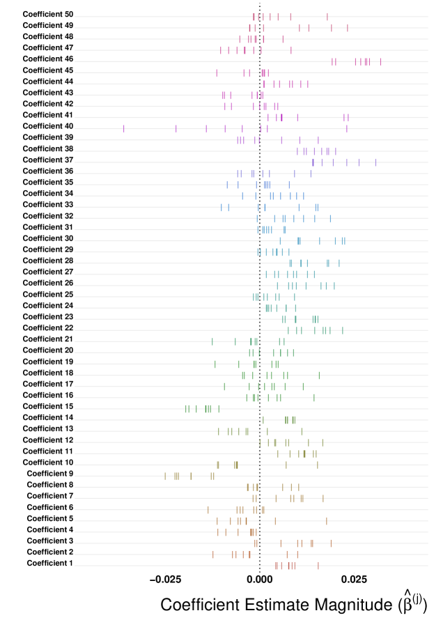
Figure G.4: Cancer genomics application rug plots displaying $\hat{\beta}_{k,j}$ for a random set of 50 $j$’s across the $K$ task-specific Ridge regressions ($\frac{1}{K}\sum_{k=1}^{K}|\hat{\beta}_{k,j}|$). For Coefficient $j$, each mark on the horizontal line is one of $K$ task-specific empirical estimates of the $\hat{\bm{\beta}}_{k,j}$.

References

- Anderson (1951) Anderson, T. W. (1951). Estimating Linear Restrictions on Regression Coefficients for Multivariate Normal Distributions. The Annals of Mathematical Statistics 22(3), 327 – 351.
- Argyriou and others (2007) Argyriou, Andreas, Micchelli, Charles, Pontil, Massimiliano and Ying, Yiming. (2007, 01). A spectral regularization framework for multi-task structure learning. In: Advances in Neural Information Processing Systems, Volume 20.
- Bang and others (2020) Bang, Dan, Kishida, Kenneth T, Lohrenz, Terry, White, Jason P, Laxton, Adrian W, Tatter, Stephen B, Fleming, Stephen M and Montague, P Read. (2020). Sub-second dopamine and serotonin signaling in human striatum during perceptual decision-making. Neuron 108(5), 999–1010.
- Beck and Eldar (2013) Beck, Amir and Eldar, Yonina C. (2013). Sparsity constrained nonlinear optimization: Optimality conditions and algorithms. SIAM Journal on Optimization 23(3), 1480–1509.
- Beck and Teboulle (2009) Beck, Amir and Teboulle, Marc. (2009). A fast iterative shrinkage-thresholding algorithm for linear inverse problems. SIAM journal on imaging sciences 2(1), 183–202.
- Behdin and Mazumder (2021) Behdin, Kayhan and Mazumder, Rahul. (2021). Sparse pca: A new scalable estimator based on integer programming. arXiv preprint arXiv:2109.11142 abs/2109.11142(2109.11142).
- Bertsimas and others (2016) Bertsimas, Dimitris, King, Angela and Mazumder, Rahul. (2016, 4). Best subset selection via a modern optimization lens. The Annals of Statistics 44(2), 813–852.
- Bertsimas and Van Parys (2020) Bertsimas, Dimitris and Van Parys, Bart. (2020, 2). Sparse high-dimensional regression: Exact scalable algorithms and phase transitions. The Annals of Statistics 48(1), 300–323.
- De Vito and others (2021) De Vito, Roberta, Bellio, Ruggero, Trippa, Lorenzo and Parmigiani, Giovanni. (2021). Bayesian multistudy factor analysis for high-throughput biological data. The Annals of Applied Statistics 15(4), 1723 – 1741.
- Evgeniou and others (2005) Evgeniou, Theodoros, Micchelli, Charles and Pontil, Massimiliano. (2005, 04). Learning multiple tasks with kernel methods. Journal of Machine Learning Research 6, 615–637.
- Fan and Li (2001) Fan, Jianqing and Li, Runze. (2001, 12). Variable selection via nonconcave penalized likelihood and its oracle properties. Journal of the American Statistical Association 96(456), 1348–1360.
- Fox and Weisberg (2019) Fox, John and Weisberg, Sanford. (2019). An R Companion to Applied Regression, Third edition. Thousand Oaks CA: Sage.
- Friedman and others (2010) Friedman, Jerome, Hastie, Trevor and Tibshirani, Robert. (2010). Regularization paths for generalized linear models via coordinate descent. Journal of Statistical Software 33(1), 1–22.
- Hazimeh and Mazumder (2020) Hazimeh, Hussein and Mazumder, Rahul. (2020, 2022/03/14). Fast best subset selection: Coordinate descent and local combinatorial optimization algorithms. Operations Research 68(5), 1517–1537.
- Hazimeh and others (2022) Hazimeh, Hussein, Mazumder, Rahul and Radchenko, Peter. (2022). Grouped variable selection with discrete optimization: Computational and statistical perspectives. The Annals of Statistics.
- Hernandez-Lobato and others (2015) Hernandez-Lobato, Daniel, Hernandez-Lobato, Jose Miguel and Ghahramani, Zoubin. (2015, 07–09 Jul). A probabilistic model for dirty multi-task feature selection. In: Proceedings of the 32nd International Conference on Machine Learning, Volume 37. PMLR. pp. 1073–1082.
- Hoerl and Kennard (1970) Hoerl, Arthur E. and Kennard, Robert W. (1970). Ridge regression: Biased estimation for nonorthogonal problems. Technometrics 12(1), 55–67.
- Johnson and others (2016) Johnson, Justin A., Rodeberg, Nathan T. and Wightman, R. Mark. (2016, 03). Failure of standard training sets in the analysis of fast-scan cyclic voltammetry data. ACS Chemical Neuroscience 7(3), 349–359.
- Kim and Xing (2012) Kim, Seyoung and Xing, Eric P. (2012, sep). Tree-guided group lasso for multi-response regression with structured sparsity, with an application to eQTL mapping. The Annals of Applied Statistics 6(3).
- Kishida and others (2016) Kishida, Kenneth T., Saez, Ignacio, Lohrenz, Terry, Witcher, Mark R., Laxton, Adrian W., Tatter, Stephen B., White, Jason P., Ellis, Thomas L., Phillips, Paul E. M. and Montague, P. Read. (2016). Subsecond dopamine fluctuations in human striatum encode superposed error signals about actual and counterfactual reward. Proceedings of the National Academy of Sciences 113(1), 200–205.
- Kishida and others (2011) Kishida, Kenneth T., Sandberg, Stefan G., Lohrenz, Terry, Comair, Youssef G., Sáez, Ignacio, Phillips, Paul E. M. and Montague, P. Read. (2011, 08). Sub-second dopamine detection in human striatum. PLOS ONE 6(8), 1–5.
- Liu and others (2009) Liu, Jun, Ji, Shuiwang and Ye, Jieping. (2009). Multi-task feature learning via efficient l2, 1-norm minimization. In: Proceedings of the Twenty-Fifth Conference on Uncertainty in Artificial Intelligence, UAI ’09. Arlington, Virginia, USA: AUAI Press. p. 339–348.
- Loewinger and others (2022) Loewinger, Gabriel, Patil, Prasad, Kishida, Kenneth T. and Parmigiani, Giovanni. (2022). Hierarchical resampling for bagging in multistudy prediction with applications to human neurochemical sensing. The Annals of Applied Statistics 16(4), 2145 – 2165.
- Lozano and Świrszcz (2012) Lozano, A.C. and Świrszcz, G. (2012, 01). Multi-level lasso for sparse multi-task regression. Proceedings of the 29th International Conference on Machine Learning, ICML 2012 1, 361–368.
- Mazumder and others (0) Mazumder, Rahul, Radchenko, Peter and Dedieu, Antoine. (0). Subset selection with shrinkage: Sparse linear modeling when the snr is low. Operations Research 0(0), null.
- Miller (1990) Miller, Alan. (1990). Subset Selection in Regression, Chapman & Hall/CRC Monographs on Statistics & Applied Probability. Taylor & Francis.
- Montague and others (2019) Montague, P. Read, Lohrenz, Terry, White, Jason, Moran, Rosalyn J and Kishida, Kenneth T. (2019). Random burst sensing of neurotransmitters. bioRxiv:607077.
- Moran and others (2018) Moran, Rosalyn J, Kishida, Kenneth T, Lohrenz, Terry, Saez, Ignacio, Laxton, Adrian W, Witcher, Mark R, Tatter, Stephen B, Ellis, Thomas L, Phillips, Paul Em, Dayan, Peter and others. (2018, 05). The protective action encoding of serotonin transients in the human brain. Neuropsychopharmacology 43(6), 1425–1435.
- Natarajan (1995) Natarajan, Balas Kausik. (1995). Sparse approximate solutions to linear systems. SIAM journal on computing 24(2), 227–234.
- Pong and others (2010) Pong, Ting Kei, Tseng, Paul, Ji, Shuiwang and Ye, Jieping. (2010). Trace norm regularization: Reformulations, algorithms, and multi-task learning. SIAM Journal on Optimization 20(6), 3465–3489.
- Raskutti and others (2011) Raskutti, G., Wainwright, M. J. and Yu, B. (2011). Minimax rates of estimation for high-dimensional linear regression over -balls. IEEE Trans. on Information Theory 57(10), 6976–6994.
- Rigollet and Hütter (2015) Rigollet, Phillippe and Hütter, Jan-Christian. (2015). High dimensional statistics. Lecture notes for course 18S997 813(814), 46.
- Suk and others (2016) Suk, Heung-Il, Lee, Seong-Whan, Shen, Dinggang and Initiative, Alzheimer’s Disease Neuroimaging. (2016, 06). Deep sparse multi-task learning for feature selection in alzheimer’s disease diagnosis. Brain structure & function 221(5), 2569–2587.
- Tibshirani (1996) Tibshirani, Robert. (1996). Regression shrinkage and selection via the lasso. Journal of the Royal Statistical Society: Series B (Methodological) 58(1), 267–288.
- Wainwright (2019) Wainwright, Martin J. (2019). High-dimensional statistics: A non-asymptotic viewpoint, Volume 48. Cambridge University Press.
- Wang and others (2014) Wang, Xin, Bi, Jinbo, Yu, Shipeng, Sun, Jiangwen and Song, Minghu. (2014). Multiplicative multitask feature learning. Journal of Machine Learning Research : JMLR 17.
- Yeo and Johnson (2000) Yeo, In-Kwon and Johnson, Richard A. (2000). A new family of power transformations to improve normality or symmetry. Biometrika 87(4), 954–959.
- Yoon and others (2021) Yoon, Chang Ho, Torrance, Robert and Scheinerman, Naomi. (2021). Machine learning in medicine: should the pursuit of enhanced interpretability be abandoned? Journal of Medical Ethics.
- Yuan and others (2016) Yuan, Han, Paskov, Ivan, Paskov, Hristo, González, Alvaro J. and Leslie, Christina S. (2016). Multitask learning improves prediction of cancer drug sensitivity. Scientific Reports 6(1), 31619.
- Yuan and Lin (2006) Yuan, Ming and Lin, Yi. (2006, 02). Model selection and estimation in regression with grouped variables. Journal of the Royal Statistical Society Series B 68, 49–67.
- Zhang (2006) Zhang, Fuzhen. (2006). The Schur complement and its applications, Volume 4. Springer Science & Business Media.
- Zhang and others (2019) Zhang, Jiashuai, Miao, Jianyu, Zhao, Kun and Tian, Yingjie. (2019). Multi-task feature selection with sparse regularization to extract common and task-specific features. Neurocomputing 340, 76–89.
- Zhang and Yang (2017) Zhang, Yu and Yang, Qiang. (2017, 07). A survey on multi-task learning. IEEE Transactions on Knowledge and Data Engineering PP.
- Zhang and others (2010) Zhang, Yu, Yeung, Dit-Yan and Xu, Qian. (2010). Probabilistic multi-task feature selection. In: Advances in Neural Information Processing Systems, Volume 23.