Hard Sample Aware Network for Contrastive Deep Graph Clustering

Abstract

Contrastive deep graph clustering, which aims to divide nodes into disjoint groups via contrastive mechanisms, is a challenging research spot. Among the recent works, hard sample mining-based algorithms have achieved great attention for their promising performance. However, we find that the existing hard sample mining methods have two problems as follows. 1) In the hardness measurement, the important structural information is overlooked for similarity calculation, degrading the representativeness of the selected hard negative samples. 2) Previous works merely focus on the hard negative sample pairs while neglecting the hard positive sample pairs. Nevertheless, samples within the same cluster but with low similarity should also be carefully learned. To solve the problems, we propose a novel contrastive deep graph clustering method dubbed Hard Sample Aware Network (HSAN) by introducing a comprehensive similarity measure criterion and a general dynamic sample weighing strategy. Concretely, in our algorithm, the similarities between samples are calculated by considering both the attribute embeddings and the structure embeddings, better revealing sample relationships and assisting hardness measurement. Moreover, under the guidance of the carefully collected high-confidence clustering information, our proposed weight modulating function will first recognize the positive and negative samples and then dynamically up-weight the hard sample pairs while down-weighting the easy ones. In this way, our method can mine not only the hard negative samples but also the hard positive sample, thus improving the discriminative capability of the samples further. Extensive experiments and analyses demonstrate the superiority and effectiveness of our proposed method. The source code of HSAN is shared at https://github.com/yueliu1999/HSAN and a collection (papers, codes and, datasets) of deep graph clustering is shared at https://github.com/yueliu1999/Awesome-Deep-Graph-Clustering on Github.

Introduction

In recent years, contrastive learning has achieved promising performance in the field of deep graph clustering benefiting from the powerful potential supervision information extraction capability (Liu et al. 2022c; Gong et al. 2022). Among the recent works, researchers demonstrate the effectiveness of hard negative sample mining in contrastive learning. Concretely, GDCL (Zhao et al. 2021) is proposed to correct the bias of the negative sample selection via clustering pseudo labels. ProGCL (Xia et al. 2022a) first filters the false negative samples and then generates a more abundant negative sample set by the sample interpolation.

Although verified to be effective, we point out two drawbacks in the existing methods as follows. 1) While measuring the hardness of samples, the important structural information is neglected for the sample similarity calculation, degrading the representativeness of the selected hard negative samples. 2) Previous works only focus on the hard negative samples while overlooking the hard positive samples, limiting the discriminative capability of samples. We argue that the samples within the same cluster but with low similarity should also be carefully learned.

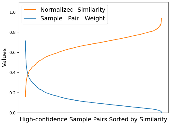
(a) Positive Sample Pairs

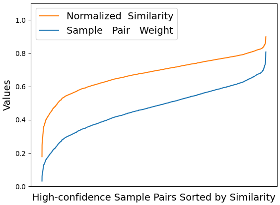
(b) Negative Sample Pairs

Figure 1: Sample weighing strategy illustration. In the sample weighting process, according to the high-confidence pseudo labels generated by the integrated clustering procedure, samples from the same clusters are recognized as potential positive sample pairs. Meanwhile, samples from different clusters are combined as potential negative sample pairs. To drive the network to focus more on the hard samples, we assign larger weights to the positive sample pairs with smaller similarities shown in sub-figure (a) and assign smaller weights to the negative sample pairs with small similarities shown in sub-figure (b). In this way, samples in the same cluster with low similarity and those in different clusters with large similarity are mined as hard samples.

To solve the mentioned problems, we propose a novel contrastive deep graph clustering method termed Hard Sample Aware Network (HSAN) by designing a comprehensive similarity measure criterion and a general dynamic sample weighting strategy. Concretely, to provide a more reliable hardness measure criterion, the sample similarity is calculated by a learnable linear combination of the attribute similarity and the structural similarity. Besides, a novel contrastive sample weighting strategy is proposed to improve the discriminative capability of the network. Firstly, we perform the clustering algorithm on the consensus node embeddings and generate the high-confidence clustering pseudo labels. Then, samples from the same clusters are recognized as potential positive sample pairs and those from different clusters are selected as potential negative ones. Especially, an adaptive sample weighing function tunes the weights of high-confidence positive and negative sample pairs according to the training difficulty. As illustrated in Figure 1, positive sample pairs with small similarity and negative ones with large similarity are the hard samples to which more attention should be paid. The main contributions of this paper are summarized as follows.

• We propose a novel contrastive deep graph clustering termed Hard Sample Aware Network (HSAN). It guides the network to focus on both hard positive and negative sample pairs.

• To assist the hard sample mining, we design a comprehensive similarity measure criterion by considering both attribute and structure information. It better reveals the similarity between samples.

• Under the guidance of the high-confidence clustering information, the proposed sample weight modulating strategy dynamically up-weights hard sample pairs while down-weighting the easy samples, thus improving the discriminative capability of the network.

• Extensive experimental results on six datasets demonstrate the superiority and the effectiveness of our proposed method.

Related Work

Deep Graph Clustering

Deep learning has been successful in many domain including computer vision (Zhou et al. 2020; Wang et al. 2022a, 2023; Wang and Chen 2021), time series analysis (Xie et al. 2022; Meng Liu 2021, 2022; Liu et al. 2022a), bioinformatics (Xia et al. 2022b; Gao et al. 2022; Tan et al. 2022), and graph data mining (Wang et al. 2020, 2021b; Zeng et al. 2022, 2023; Wu et al. 2022; Duan et al. 2022; Yang et al. 2022b; Liang et al. 2022b). Among these directions, deep graph clustering, which aims to encode nodes with neural networks and divide them into disjoint clusters, has attracted great attention in recent years. According to the learning mechanisms, the existing methods can be roughly categorized into three classes: generative methods (Wang et al. 2017; Mrabah et al. 2022; Xia et al. 2022e), adversarial methods (Pan et al. 2019; Gong et al. 2022), and contrastive methods. More information about the fast-growing deep graph clustering can be checked in our survey paper (Liu et al. 2022d). In this work, we focus on the last category, i.e., the contrastive deep graph clustering. Recently, contrastive mechanisms have succeeded in many domains such as images (Xu and Lang 2020) and graphs (Zhu et al. 2020; Wu et al. 2021b), and knowledge graphs (Liang et al. 2022a). Inspired by their success, the contrastive deep graph clustering methods are increasingly proposed. A pioneer AGE (Cui et al. 2020) conducts contrastive learning by a designed adaptive encoder. MVGRL (Hassani and Khasahmadi 2020) adopts the InfoMax loss (Hjelm et al. 2018) to maximize the cross-view mutual information. Subsequently, SCAGC (Xia et al. 2022d) pulls together the positive samples while pushing away negative ones across augmented views. After that, DCRN and its variants (Liu et al. 2022c, f) alleviate the collapsed representation by reducing correlation in a dual manner. Then SCGC (Liu et al. 2022e) is proposed to reduce high time cost of the existing methods by simplifying the data augmentation and the graph convolutional operation. More recently, the selection of positive and negative samples has attracted great attention. Concretely, GDCL (Zhao et al. 2021) develops a debiased sampling strategy to correct the bias for negative samples. However, most of the existing methods treat the easy and hard samples equally, leading to indiscriminative capability. To solve this problem, we propose a novel contrastive deep graph clustering by mining the hard samples. In our proposed method, the weights of the hard positive and negative samples will dynamically increased while the weights of the easy ones will be decreased.

Hard Sample Mining

In the contrastive learning methods, one key factor of promising performance is the positive and negative sample selection. Previous works (Chuang et al. 2020; Robinson et al. 2020; Kalantidis et al. 2020) on images have demonstrated that the hard negative samples are hard yet useful. Motivated by their success, more researchers take attention to the hard negative sample mining on graphs. Concretely, GDCL (Zhao et al. 2021) utilizes the clustering pseudo labels to correct the bias of the negative sample selection in the attribute graph clustering task. Besides, CuCo (Chu et al. 2021) selects and learns the samples from easy to hard in the graph classification task. In addition, to better mine true and hard negative samples, STENCIL (Zhu et al. 2022) advocates enriching the model with local structure patterns of heterogeneous graphs. More recently, ProGCL (Xia et al. 2022a) built a more suitable measure for the hardness of negative samples together with similarity by a designed probability estimator. Although verified the effectiveness, previous methods neglect the hard positive sample pair, thus leading to sub-optimal performance. In this work, we argue that the samples with the same category but low similarity should also be carefully learned. From this motivation, we propose a general sample weighting strategy to guide the network focus more on both the hard positive and negative samples.

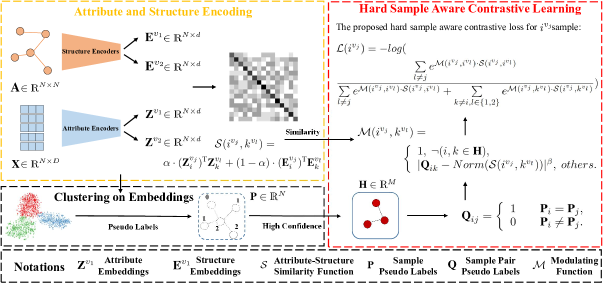
Figure 2: Illustration of our proposed hard sample aware network. In attribute and structure encoding, we embed the attribute and structure into the latent space with the attribute encoders and structure encoders. Then the sample similarities are calculated by a learnable linear combination of attribute similarity and structure similarity, thus better revealing the sample relations. Moreover, guided by the high-confidence information, a general dynamic sample weighting strategy is proposed to up-weight hard sample pairs while down-weighting the easy ones. Overall, the hard sample aware contrastive loss guides the network to focus more on both hard positive and negative sample pairs, thus further improving the discriminative capability of samples.

Method

In this section, we propose a novel Hard Sample Aware Network (HSAN) for contrastive deep graph clustering by guiding our network to focus on both the hard positive and negative sample pairs. The framework is shown in Figure 2.

Notation and Problem Definition

Let $\mathcal{V}=\{v_{1},v_{2},\dots,v_{N}\}$ be a set of $N$ nodes with $C$ classes and $\mathcal{E}$ be a set of edges. In the matrix form, $\textbf{X}\in\mathds{R}^{N\times D}$ and $\textbf{A}\in\mathds{R}^{N\times N}$ denotes the attribute matrix and the original adjacency matrix, respectively. Then $\mathcal{G}=\left\{\textbf{X},\textbf{A}\right\}$ denotes an undirected graph. The degree matrix is formulated as $\textbf{D}=diag(d_{1},d_{2},\dots,d_{N})\in\mathds{R}^{N\times N}$ and $d_{i}=\sum_{(v_{i},v_{j})\in\mathcal{E}}a_{ij}$. The graph Laplacian matrix is defined as $\textbf{L}=\textbf{D}-\textbf{A}$. With the renormalization trick $\widehat{\textbf{A}}=\textbf{A}+\textbf{I}$ in GCN (Kipf and Welling 2017), the symmetric normalized graph Laplacian matrix is denoted as $\widetilde{\textbf{L}}=\textbf{I}-\widehat{\textbf{D}}^{-\frac{1}{2}}\widehat{\textbf{A}}\widehat{\textbf{D}}^{-\frac{1}{2}}$. The notations are summarized in Table 1.

The target of deep graph clustering is to encode nodes with the neural network in an unsupervised manner and then divide them into several disjoint groups. In general, a neural network $\mathcal{F}$ is firstly trained without human annotations and embeds the nodes into the latent space by exploiting the node attributes and the graph structure as follows:

$$\textbf{E}=\mathcal{F}(\textbf{A},\textbf{X}),$$ (1)

where X and A denotes the attribute matrix and the original adjacency matrix. Besides, $\textbf{E}\in\mathds{R}^{N\times d}$ is the learned node embeddings, where $N$ is the number of samples and $d$ is the number of feature dimensions. After that, a clustering algorithm $\mathcal{C}$ such as K-means, spectral clustering, or the clustering neural network layer (Bo et al. 2020) is adopted to divide nodes into $K$ disjoint groups as follows:

$$\Phi=\mathcal{C}(\textbf{E}),$$ (2)

where $\Phi\in\mathds{R}^{N\times K}$ denotes the cluster membership matrix for all $N$ samples.

Notation	Meaning
$\textbf{X}\in\mathds{R}^{N\times D}$	Attribute matrix
$\widetilde{\textbf{X}}\in\mathds{R}^{N\times D}$	Low-pass filtered attribute matrix
$\textbf{A}\in\mathds{R}^{N\times N}$	Original adjacency matrix
$\widehat{\textbf{A}}\in\mathds{R}^{N\times N}$	Adjacency matrix with self-loop
$\textbf{L}\in\mathds{R}^{N\times N}$	Graph Laplacian matrix
$\widetilde{\textbf{L}}\in\mathds{R}^{N\times N}$	Symmetric normalized Laplacian matrix
$\textbf{Z}^{v_{k}}\in\mathds{R}^{N\times d}$	Attribute embeddings in $k$-th view
$\textbf{E}^{v_{k}}\in\mathds{R}^{N\times d}$	Structure embeddings in $k$-th view
$\textbf{P}\in\mathds{R}^{N}$	Sample clustering pseudo labels
$\textbf{H}\in\mathds{R}^{M}$	High-confidence sample set
$\textbf{Q}\in\mathds{R}^{N\times N}$	Sample pair pseudo labels
$\|\cdot\|_{2}$	L-2 norm

Table 1: Notation summary.

Attribute and Structure Encoding

In this section, we design two types of encoders to embed the nodes into the latent space. Concretely, the attribute encoder (AE) and the structure encoder (SE) encode the attribute and structural information of samples, respectively.

In the process of attribute encoding, we follow previous work (Cui et al. 2020) and filter the high-frequency noises in the attribute matrix $\widetilde{\textbf{X}}$ as formulated:

$$\widetilde{\textbf{X}}=(\prod_{i=1}^{t}(\textbf{I}-\widetilde{\textbf{L}}))\textbf{X}=(\textbf{I}-\widetilde{\textbf{L}})^{t}\textbf{X},$$ (3)

where $\textbf{I}-\widetilde{\textbf{L}}$ is the graph Laplacian filter and $t$ is the filtering times. Then we encode $\widetilde{\textbf{X}}$ with $\text{AE}_{1}$ and $\text{AE}_{2}$ as follows:

$$\textbf{Z}^{v_{1}} =\text{AE}_{1}(\widetilde{\textbf{X}});\textbf{Z}^{v_{1}}_{i}=\frac{\textbf{Z}^{v_{1}}_{i}}{||\textbf{Z}^{v_{1}}_{i}||_{2}},i=1,2,...,N;$$ (4)

$$\textbf{Z}^{v_{2}} =\text{AE}_{2}(\widetilde{\textbf{X}});\textbf{Z}^{v_{2}}_{j}=\frac{\textbf{Z}^{v_{2}}_{j}}{||\textbf{Z}^{v_{2}}_{j}||_{2}},j=1,2,...,N,$$

where $\textbf{Z}^{v_{1}}$ and $\textbf{Z}^{v_{2}}$ denote two-view attribute embeddings of the samples. Here, $\text{AE}_{1}$ and $\text{AE}_{2}$ are both simple multi-layer perceptions (MLPs), which have the same architecture but un-shared parameters, thus $\textbf{Z}^{v_{1}}$ and $\textbf{Z}^{v_{2}}$ contain different semantic information. Different the mixup-based methods (Yang et al. 2022a; Wu et al. 2021a), our proposed method is free from augmentation.

In addition, we further propose the structure encoder to encode the structural information of samples. Concretely, we design the structure encoder as follows:

$$\textbf{E}^{v_{1}} =\text{SE}_{1}(\textbf{A});\textbf{E}^{v_{1}}_{i}=\frac{\textbf{E}^{v_{1}}_{i}}{||\textbf{E}^{v_{1}}_{i}||_{2}},i=1,2,...,N;$$ (5)

$$\textbf{E}^{v_{2}} =\text{SE}_{2}(\textbf{A});\textbf{E}^{v_{2}}_{j}=\frac{\textbf{E}^{v_{2}}_{j}}{||\textbf{E}^{v_{2}}_{j}||_{2}},j=1,2,...,N,$$

where $\textbf{E}^{v_{1}}$ and $\textbf{E}^{v_{2}}$ denote two-view structure embeddings. Similarly, $\text{SE}_{1}$ and $\text{SE}_{2}$ are simple MLPs, which have the same architecture but un-shared parameters, thus $\textbf{E}^{v_{1}}$ and $\textbf{E}^{v_{2}}$ contain different semantic information during training.

In this manner, we obtain the attribute embedding and structure embedding of each sample. Subsequently, the attribute-structure similarity function $\mathcal{S}$ is proposed to calculate the similarity between $i$-th sample in the $j$-th view and $k$-th sample in the $l$-th view as formulated:

$$\mathcal{S}(i^{v_{j}},k^{v_{l}})=\alpha\cdot(\textbf{Z}_{i}^{v_{j}})^{\text{T}}\textbf{Z}_{k}^{v_{l}}+(1-\alpha)\cdot(\textbf{E}_{i}^{v_{j}})^{\text{T}}\textbf{E}_{k}^{v_{l}},$$ (6)

where $i,k\in\{1,2,...,N\}$ and $j,l\in\{1,2\}$. Besides, $\alpha$ denotes a learnable trade-off parameter. The first and second term in Eq. (6) both denotes the cosine similarity. $\mathcal{S}$ can better reveal sample relations by considering both attribute and structure information, thus assisting the hard sample mining.

Clustering and Pseudo Label Generation

After encoding, K-means is performed on the learned node embeddings to obtain the clustering results. Then we extract the more reliable clustering information as follows. To be specific, we first generate the clustering pseudo labels $\textbf{P}\in\mathds{R}^{N}$ and then select the top $\tau$ samples as the high-confidence sample set $\textbf{H}\in\mathds{R}^{M}$. Here, $\tau$ is the confidence hyper-parameter and $M$ is the number of high-confidence samples. The confidence is measured by the distance to the cluster center (Liu et al. 2022f). Based on P, we calculate the sample pair pseudo labels $\textbf{Q}\in\mathds{R}^{N\times N}$ as follows:

$$\textbf{Q}_{ij}=\left\{\begin{array}[]{rcl}1&&{\textbf{P}_{i}=\textbf{P}_{j}},\\ 0&&{\textbf{P}_{i}\neq\textbf{P}_{j}}.\end{array}\right.$$ (7)

Here, $\textbf{Q}_{ij}$ reveals the pseudo relation between $i$-th and $j$-th samples. Precisely, $\textbf{Q}_{ij}=1$ means $i-th$ and $j$-th samples are more likely to be the positive sample pair while $\textbf{Q}_{ij}=0$ implies they are more likely to be the negative ones.

Hard Sample Aware Contrastive Learning

In this section, we firstly introduce the drawback of classical infoNCE loss (Van den Oord et al. 2018) in the graph contrastive methods (Zhu et al. 2020; Xia et al. 2022a) and then propose a novel hard sample aware contrastive loss to guide our network to focus more on hard positive and negative samples.

The classical infoNCE loss for $i$-th sample in the $j$-th view is formulated as follows:

$$\mathcal{L}_{infoNCE}(i^{v_{j}})=$$ (8)

$$-log\frac{e^{\theta(i^{v_{j}},i^{v_{l}})}}{e^{\theta(i^{v_{j}},i^{v_{l}})}+\sum\limits_{k\neq i}({e^{\theta(i^{v_{j}},k^{v_{j}})}}+e^{\theta(i^{v_{j}},k^{v_{l}})})}.$$

where $j\neq l$. Besides, $\theta(\cdot)$ denotes the cosine similarity between the paired samples in the latent space. By minimizing infoNCE loss, they pull together the same samples in different views while pushing away other samples.

However, we find the drawback of classical infoNCE is that the hard sample pairs are treated equally to the easy ones, limiting the discriminative capability of the network. To solve this problem, we propose a weight modulating function $\mathcal{M}$ to dynamically adjust the weights of sample pairs during training. Concretely, based on the proposed attribute-structure similarity function $\mathcal{S}$ and the generated sample pair pseudo labels Q, $\mathcal{M}$ is formulated as follows:

$$\mathcal{M}(i^{v_{j}},k^{v_{l}})=\left\{\begin{array}[]{l}1,\ \neg(i,k\in\textbf{H}),\\ |\textbf{Q}_{ik}-Norm(\mathcal{S}(i^{v_{j}},k^{v_{l}}))|^{\beta},\ others.\end{array}\right.$$ (9)

where $i^{v_{j}}$ denotes the $i$-th samples in the $j$-th view and $Norm$ denotes the min-max normalization. In Eq. (9), when $i$-th or $j$-th sample is not with high-confidence, i.e., $\neg(i,k\in\textbf{H})$, we keep the original setting in the infoNCE loss. Differently, the sample weights are modulated with the pseudo information and the similarity of samples, when the samples are with high-confidence. Here, the hyper-parameter $\beta\in[1,\ 5]$ is the focusing factor, which determines the down-weighting rate of the easy sample pairs. In the following, we analyze the properties of the proposed weight modulating function $\mathcal{M}$.

1) $\mathcal{M}$ can up-weight the hard samples while down-weighting the easy samples. Concretely, when $i$-th, $j$-th samples are recognized as positive sample pair ($\textbf{Q}_{ij}=1$), the hardness of pulling them together decreases as the similarity increases. Thus, $\mathcal{M}$ up-weights the positive sample pairs with small similarity (the hard ones) while down-weighting that with large similarity (the easy ones). For example, when $\textbf{Q}_{ij}=1$ and $\beta=2$, the easy positive sample pair with $0.90$ similarity is weighted with $0.01$. Differently, the hard positive sample pair with $0.10$ similarity is weighted with $0.81$, which is significantly larger than $0.01$. The similar conclusion can be deduced on the negative sample pairs. Experimental evidence can be found in Figure 1.

2) The focusing factor $\beta$ controls the down-weighting rate of easy sample pairs. Concretely, when $\beta$ increases, the down-weighting rate of easy sample pairs increases and vice versa. Take the positive sample pair as an example ($\textbf{Q}_{ij}=1$), the easy ones with $0.9$ similarity be down-weighted to $0.1^{\beta}$. Here, when $\beta=1$, the weight is set to $0.1$. Differently, when $\beta=3$, the weight is degraded to $0.001$, which is obviously smaller than $0.1$. This property is verified by visualization experiments in Figure 2-3 of Appendix.

Based on $\mathcal{S}$ and $\mathcal{M}$, we formulate the hard sample aware contrastive loss for $i$-th sample in $j$-th view as follows:

$$\mathcal{L}(i^{v_{j}})=-log($$ (10)

$$\frac{\sum\limits_{l\neq j}e^{\mathcal{M}(i^{v_{j}},i^{v_{l}})\cdot\mathcal{S}(i^{v_{j}},i^{v_{l}})}}{\sum\limits_{l\neq j}e^{\mathcal{M}(i^{v_{j}},i^{v_{l}})\cdot\mathcal{S}(i^{v_{j}},i^{v_{l}})}+\sum\limits_{k\neq i,l\in\{1,2\}}{e^{\mathcal{M}(i^{v_{j}},k^{v_{l}})\cdot\mathcal{S}(i^{v_{j}},k^{v_{l}})}}}).$$

Compared with the classical infoNCE loss, we first adopt a more comprehensive similarity measure criterion $\mathcal{S}$ to assist sample hardness measurement. Then we propose a weight modulating function $\mathcal{M}$ to up-weight hard sample pairs and down-weight the easy ones. In summary, the overall loss of our method is formulated as follows:

$$\mathcal{L}=\frac{1}{2N}\sum_{j=1}^{2}\sum_{i=1}^{N}\mathcal{L}(i^{v_{j}}).$$ (11)

This hard sample aware contrastive loss can guide our network to focus on not only the hard negative samples but also the hard positive ones, thus improving the discriminative capability of samples further. We summarize two reasons as follows. 1) The proposed attribute-structure similarity function $\mathcal{S}$ considers attribute and structure information, thus better revealing the sample relations. 2) The proposed weight modulating function $\mathcal{M}$ is a general dynamic sample weighting strategy for positive and negative sample pairs. It can up-weight the hard sample pairs while down-weighting the easy ones during training.

Complexity Analysis of Loss Function

In this section, we analyze the time and space complexity of the proposed hard sample aware contrastive loss $\mathcal{L}$. Here, we denote the batch size is $B$, the number of the high confident samples in this batch is $M$, and the dimension of embeddings is $d$. The time complexity of $\mathcal{S}$ and $\mathcal{M}$ is $\mathcal{O}(B^{2}d)$ and $\mathcal{O}(M^{2}d)$, respectively. Since $M<B$, the time complexity of the whole hard sample aware contrastive loss is $\mathcal{O}(B^{2}d)$. Besides, the space complexity of our proposed loss is $\mathcal{O}(B^{2})$. Thus, the proposed loss will not bring the high time or space costs compared with the classical infoNCE loss. The detailed process of our proposed HSAN is summarized in Algorithm 1. Besides, the PyTorch-style pseudo code can be found in Appendix.

Algorithm 1 Hard Sample Aware Network

Experiments

Dataset

To evaluate the effectiveness of our proposed HSAN, we conduct experiments on six benchmark datasets, including CORA, CITE, Amazon Photo (AMAP), Brazil Air-Traffic (BAT), Europe Air-Traffic (EAT), and USA Air-Traffic (UAT). The brief information of datasets is summarized in Table 1 of the Appendix.

Classical Deep Graph Clustering

Contrastive Deep Graph Clustering

Hard Sample Mining

MGAE

DAEGC

ARGA

SDCN

DFCN

AGE

MVGRL

AutoSSL

AGC-DRR

DCRN

AFGRL

GDCL

ProGCL

HSAN

Dataset

Metric

CIKM 19

IJCAI 19

IJCAI 19

WWW 20

AAAI 21

SIGKDD 20

ICML 20

ICLR 22

IJCAI 22

AAAI 22

AAAI 22

IJCAI 21

ICML 22

Ours

ACC

43.38±2.11

70.43±0.36

71.04±0.25

35.60±2.83

36.33±0.49

73.50±1.83

70.47±3.70

63.81±0.57

40.62±0.55

61.93±0.47

26.25±1.24

70.83±0.47

57.13±1.23

77.07±1.56

NMI

28.78±2.97

52.89±0.69

51.06±0.52

14.28±1.91

19.36±0.87

57.58±1.42

55.57±1.54

47.62±0.45

18.74±0.73

45.13±1.57

12.36±1.54

56.60±0.36

41.02±1.34

59.21±1.03

ARI

16.43±1.65

49.63±0.43

47.71±0.33

07.78±3.24

04.67±2.10

50.10±2.14

48.70±3.94

38.92±0.77

14.80±1.64

33.15±0.14

14.32±1.87

48.05±0.72

30.71±2.70

57.52±2.70

CORA

F1

33.48±3.05

68.27±0.57

69.27±0.39

24.37±1.04

26.16±0.50

69.28±1.59

67.15±1.86

56.42±0.21

31.23±0.57

49.50±0.42

30.20±1.15

52.88±0.97

45.68±1.29

75.11±1.40

ACC

61.35±0.80

64.54±1.39

61.07±0.49

65.96±0.31

69.50±0.20

69.73±0.24

62.83±1.59

66.76±0.67

68.32±1.83

70.86±0.18

31.45±0.54

66.39±0.65

65.92±0.80

71.15±0.80

NMI

34.63±0.65

36.41±0.86

34.40±0.71

38.71±0.32

43.90±0.20

44.93±0.53

40.69±0.93

40.67±0.84

43.28±1.41

45.86±0.35

15.17±0.47

39.52±0.38

39.59±0.39

45.06±0.74

ARI

33.55±1.18

37.78±1.24

34.32±0.70

40.17±0.43

45.50±0.30

45.31±0.41

34.18±1.73

38.73±0.55

45.34±2.33

47.64±0.30

14.32±0.78

41.07±0.96

36.16±1.11

47.05±1.12

CITE

F1

57.36±0.82

62.20±1.32

58.23±0.31

63.62±0.24

64.30±0.20

64.45±0.27

59.54±2.17

58.22±0.68

64.82±1.60

65.83±0.21

30.20±0.71

61.12±0.70

57.89±1.98

63.01±1.79

ACC

71.57±2.48

75.96±0.23

69.28±2.30

53.44±0.81

76.82±0.23

75.98±0.68

41.07±3.12

54.55±0.97

76.81±1.45

75.51±0.77

43.75±0.78

51.53±0.38

77.02±0.33

NMI

62.13±2.79

65.25±0.45

58.36±2.76

44.85±0.83

66.23±1.21

65.38±0.61

30.28±3.94

48.56±0.71

66.54±1.24

64.05±0.15

37.32±0.28

39.56±0.39

67.21±0.33

ARI

48.82±4.57

58.12±0.24

44.18±4.41

31.21±1.23

58.28±0.74

55.89±1.34

18.77±2.34

26.87±0.34

60.15±1.56

54.45±0.48

21.57±0.51

34.18±0.89

58.01±0.48

AMAP

F1

68.08±1.76

69.87±0.54

64.30±1.95

50.66±1.49

71.25±0.31

71.74±0.93

32.88±5.50

54.47±0.83

71.03±0.64

OOM

69.99±0.34

38.37±0.29

31.97±0.44

72.03±0.46

ACC

53.59±2.04

52.67±0.00

67.86±0.80

53.05±4.63

55.73±0.06

56.68±0.76

37.56±0.32

42.43±0.47

47.79±0.02

67.94±1.45

50.92±0.44

45.42±0.54

55.73±0.79

77.15±0.72

NMI

30.59±2.06

21.43±0.35

49.09±0.54

25.74±5.71

48.77±0.51

36.04±1.54

29.33±0.70

17.84±0.98

19.91±0.24

47.23±0.74

27.55±0.62

31.70±0.42

28.69±0.92

53.21±0.93

ARI

24.15±1.70

18.18±0.29

42.02±1.21

21.04±4.97

37.76±0.23

26.59±1.83

13.45±0.03

13.11±0.81

14.59±0.13

39.76±0.87

21.89±0.74

19.33±0.57

21.84±1.34

52.20±1.11

BAT

F1

50.83±3.23

52.23±0.03

67.02±1.15

46.45±5.90

50.90±0.12

55.07±0.80

29.64±0.49

34.84±0.15

42.33±0.51

67.40±0.35

46.53±0.57

39.94±0.57

56.08±0.89

77.13±0.76

ACC

44.61±2.10

36.89±0.15

52.13±0.00

39.07±1.51

49.37±0.19

47.26±0.32

32.88±0.71

31.33±0.52

37.37±0.11

50.88±0.55

37.42±1.24

33.46±0.18

43.36±0.87

56.69±0.34

NMI

15.60±2.30

05.57±0.06

22.48±1.21

08.83±2.54

32.90±0.41

23.74±0.90

11.72±1.08

07.63±0.85

07.00±0.85

22.01±1.23

11.44±1.41

13.22±0.33

23.93±0.45

33.25±0.44

ARI

13.40±1.26

05.03±0.08

17.29±0.50

06.31±1.95

23.25±0.18

16.57±0.46

04.68±1.30

02.13±0.67

04.88±0.91

18.13±0.85

06.57±1.73

04.31±0.29

15.03±0.98

26.85±0.59

EAT

F1

43.08±3.26

34.72±0.16

52.75±0.07

33.42±3.10

42.95±0.04

45.54±0.40

25.35±0.75

21.82±0.98

35.20±0.17

47.06±0.66

30.53±1.47

25.02±0.21

42.54±0.45

57.26±0.28

ACC

48.97±1.52

52.29±0.49

49.31±0.15

52.25±1.91

33.61±0.09

52.37±0.42

44.16±1.38

42.52±0.64

42.64±0.31

49.92±1.25

41.50±0.25

48.70±0.06

45.38±0.58

56.04±0.67

NMI

20.69±0.98

21.33±0.44

25.44±0.31

21.61±1.26

26.49±0.41

23.64±0.66

21.53±0.94

17.86±0.22

11.15±0.24

24.09±0.53

17.33±0.54

25.10±0.01

22.04±2.23

26.99±2.11

ARI

18.33±1.79

20.50±0.51

16.57±0.31

21.63±1.49

11.87±0.23

20.39±0.70

17.12±1.46

13.13±0.71

09.50±0.25

17.17±0.69

13.62±0.57

21.76±0.01

14.74±1.99

25.22±1.96

UAT

F1

47.95±1.52

50.33±0.64

50.26±0.16

45.59±3.54

25.79±0.29

50.15±0.73

39.44±2.19

34.94±0.87

35.18±0.32

44.81±0.87

36.52±0.89

45.69±0.08

39.30±1.82

54.20±1.84

Table 2: The average clustering performance of ten runs on six benchmark datasets. The performance is evaluated by four metrics with mean value and standard deviation. The red and blue values indicate the best and the runner-up results, respectively.

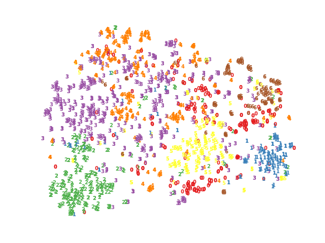
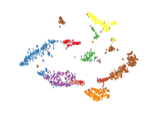
(a) DAEGC

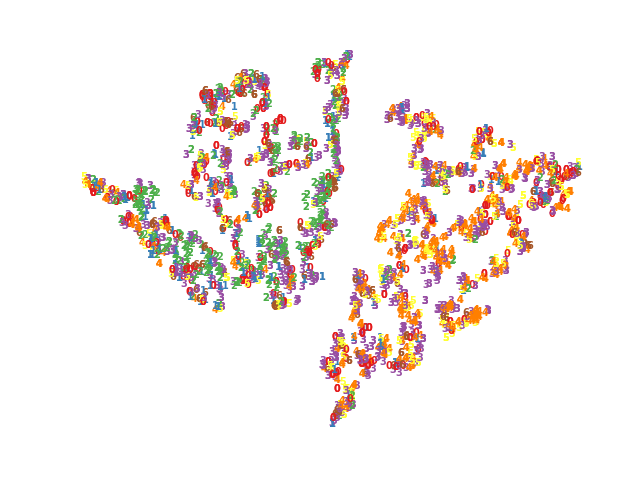
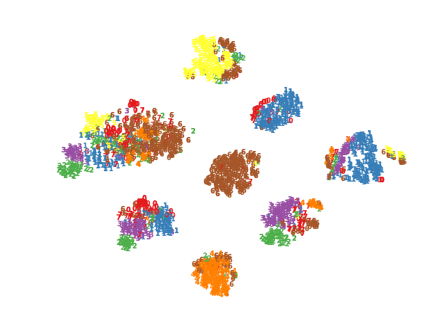
(b) SDCN

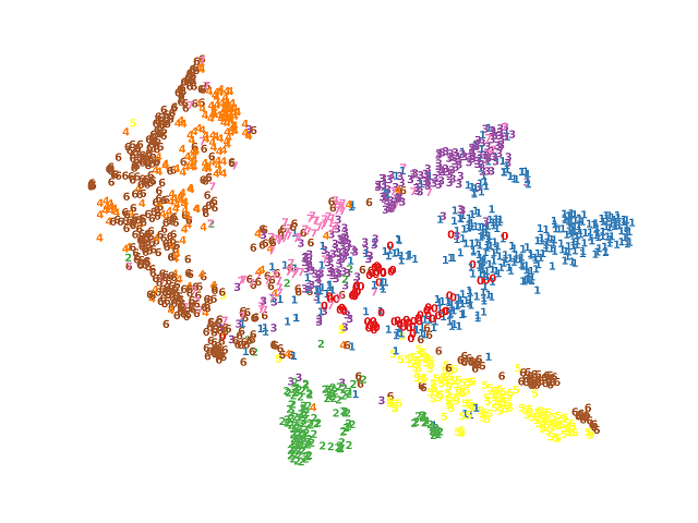
(c) AutoSSL

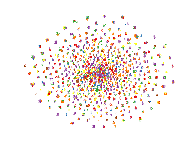
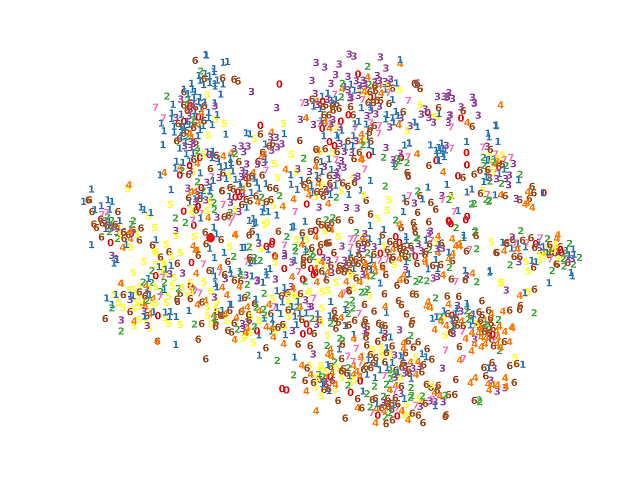
(d) AFGRL

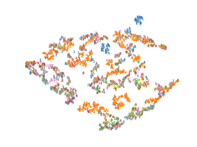
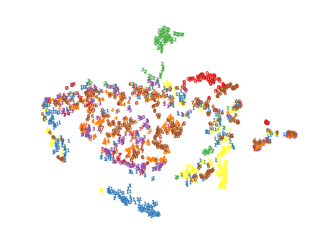
(e) GDCL

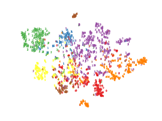
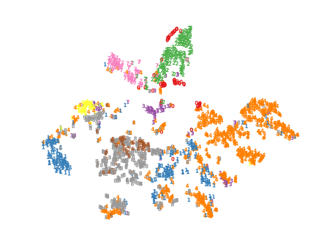
(f) ProGCL

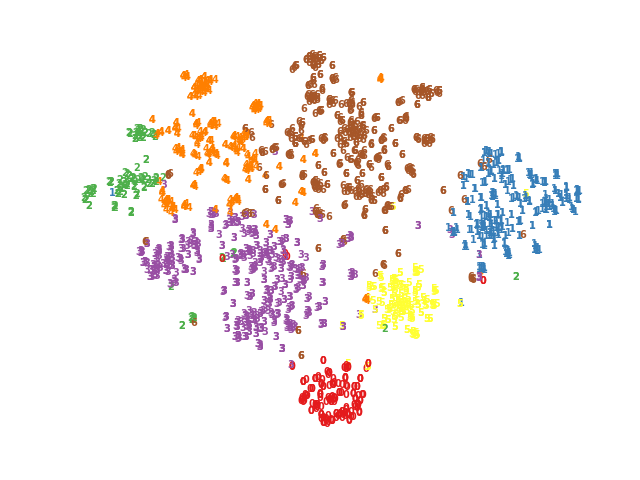
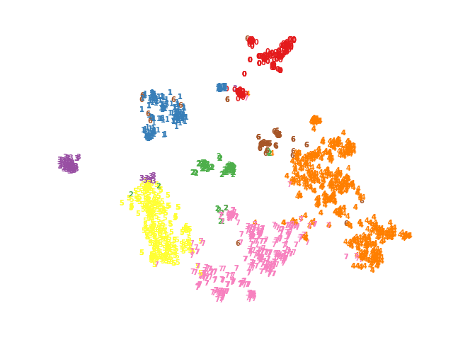
(g) Ours

Figure 3: 2D $t$-SNE visualization of seven methods on two benchmark datasets. The first row and second row corresponds to CORA and AMAP dataset, respectively.

Experimental Setup

All experimental results are obtained from the desktop computer with the Intel Core i7-7820x CPU, one NVIDIA GeForce RTX 2080Ti GPU, 64GB RAM, and the PyTorch deep learning platform. The training epoch number is set to 400 and we conduct ten runs for all methods. For the baselines, we adopt their source with original settings and reproduce the results. To our model, both the attribute encoders and structure encoders are two parameters un-shared one-layer MLPs with 500 hidden units for UAT/AMAP and 1500 hidden units for other datasets. The learnable trade-off $\alpha$ is set to $0.99999$ as initialization and reduces to around $0.4$ in our experiments as shown in Figure 4 of Appendix. The hyper-parameter settings are summarized in Table 1 of Appendix. The clustering performance is evaluated by four metrics, i.e., ACC, NMI, ARI, and F1, which are widely used in both deep clustering (Liu et al. 2022c; Xia et al. 2022c; Bo et al. 2020; Tu et al. 2020; Liu et al. 2022f) and traditional clustering (Zhou et al. 2019; Zhang et al. 2022b, 2021; Liu et al. 2022b; Chen et al. 2022b, a; Li et al. 2022; Zhang et al. 2022a, 2020; Sun et al. 2021; Wan et al. 2022; Wang et al. 2022b, 2021a).

Performance Comparison

To demonstrate the superiority of our proposed HSAN, we conduct extensive comparison experiments on six benchmark datasets. Concretely, we category these thirteen state-of-the-art deep graph clustering methods into three types, i.e., classical deep graph clustering methods (Wang et al. 2017, 2019; Bo et al. 2020; Tu et al. 2020), contrastive deep graph clustering methods (Cui et al. 2020; Hassani and Khasahmadi 2020; Gong et al. 2022; Liu et al. 2022c; Lee, Lee, and Park 2021; Jin et al. 2021), and hard sample mining methods (Zhao et al. 2021; Xia et al. 2022a). From the results in Table 2, we have three conclusions as follows. 1) Firstly, compared with the classical deep graph clustering methods, our method achieves promising performance since the contrastive mechanism helps the network capture more potential supervision information. 2) Besides, our proposed HSAN can surpass other contrastive methods thanks to our hard sample mining strategy, which guides the network to focus more the hard samples. 3) Furthermore, the existing hard sample mining methods overlook the hard positive samples and the structural information in the hardness measurement, thus limiting the discriminative capability. Take the CORA dataset as an example, our method surpasses ProGCL (Xia et al. 2022a) 18.99 % with the NMI metric. In summary, these experimental results verify the superiority of our proposed methods. Moreover, due to the limitations of paper pages, additional comparison experimental results of nine baselines can be found in Table 2 of the Appendix. The corresponding results also demonstrate the superiority of our proposed HSAN.

Ablation Study

In this section, we conduct ablation studies to verify the effectiveness of the proposed attribute-structure similarity function $\mathcal{S}$ and weight modulating function $\mathcal{M}$. Concretely, in Figure 4, we denote “B” as the baseline. In addition, “B+S”, “B+M”, and “Ours” denotes the baseline with $\mathcal{S}$, $\mathcal{M}$, and both, respectively. From the results in Figure 4, we have three observations as follows. 1) Our proposed attribute-structure similarity function $\mathcal{S}$ improves the performance of the baseline. The reason is that $\mathcal{S}$ measures the similarity between samples by considering both attribute and structure information, thus better revealing the potential relation between samples. 2) “B+M” can improve the performance of “B”. It indicates that the proposed weight modulating function $\mathcal{M}$ enhances the discriminative capability of samples by guiding our network to focus on the hard sample pairs. 3) The combination of $\mathcal{S}$ and $\mathcal{M}$ achieves the most superior clustering performance. For example, “Ours” exceeds “B” 8.48 % with the NMI metric on the CORA dataset. Overall, the effectiveness of our proposed attribute-structure similarity function $\mathcal{S}$ and weight modulating function $\mathcal{M}$ is verified by extensive experimental results.

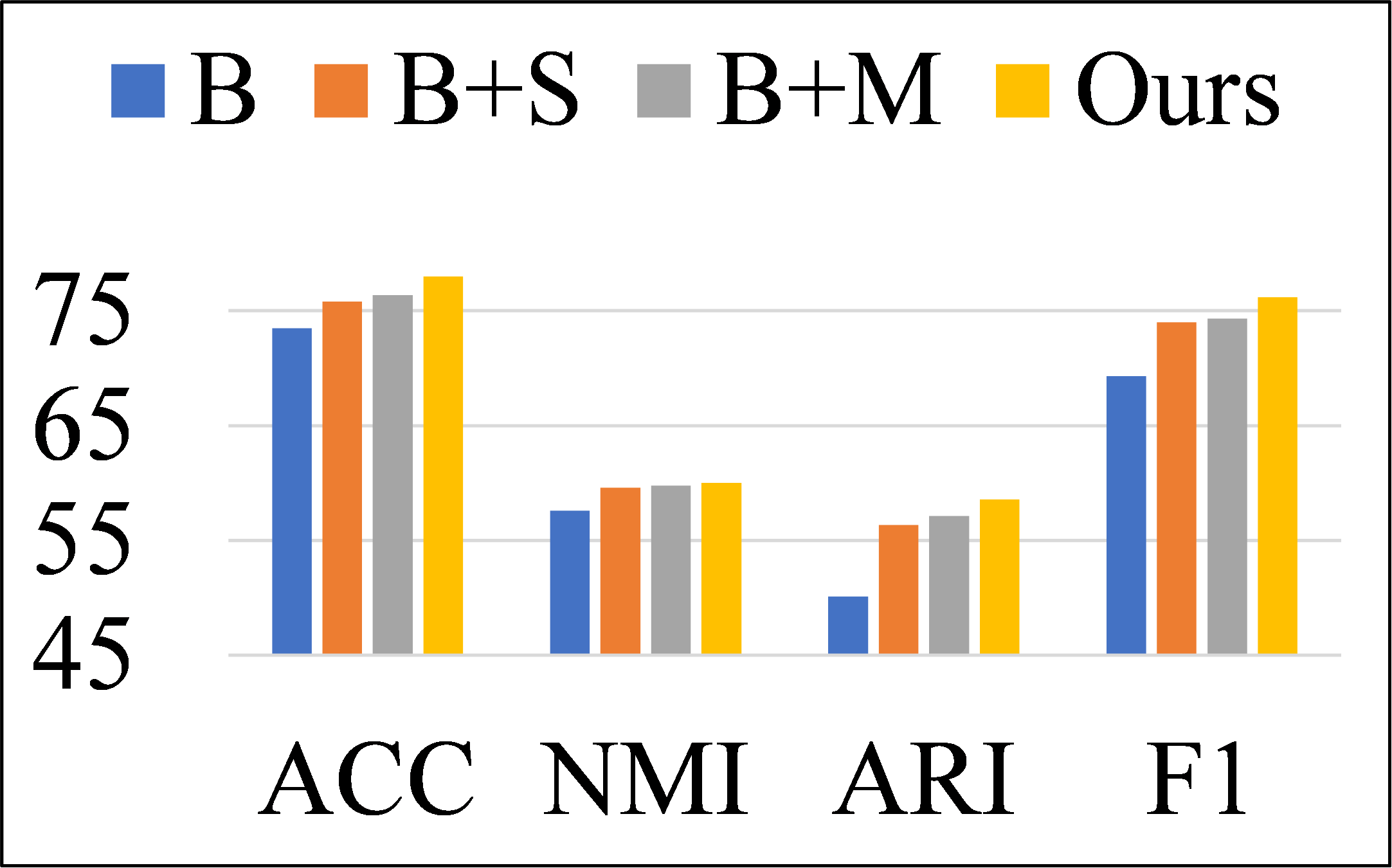
(a) CORA

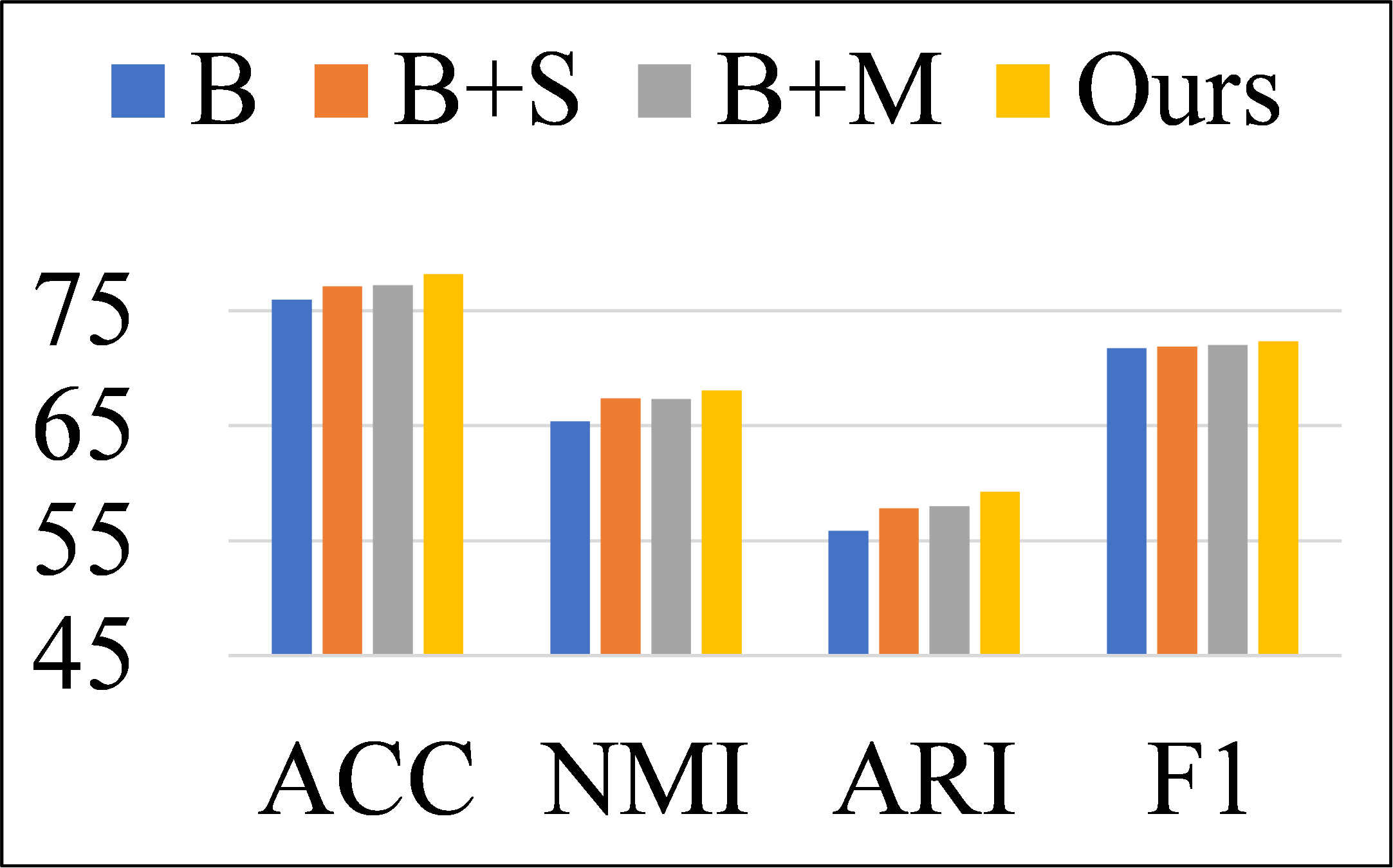
(b) AMAP

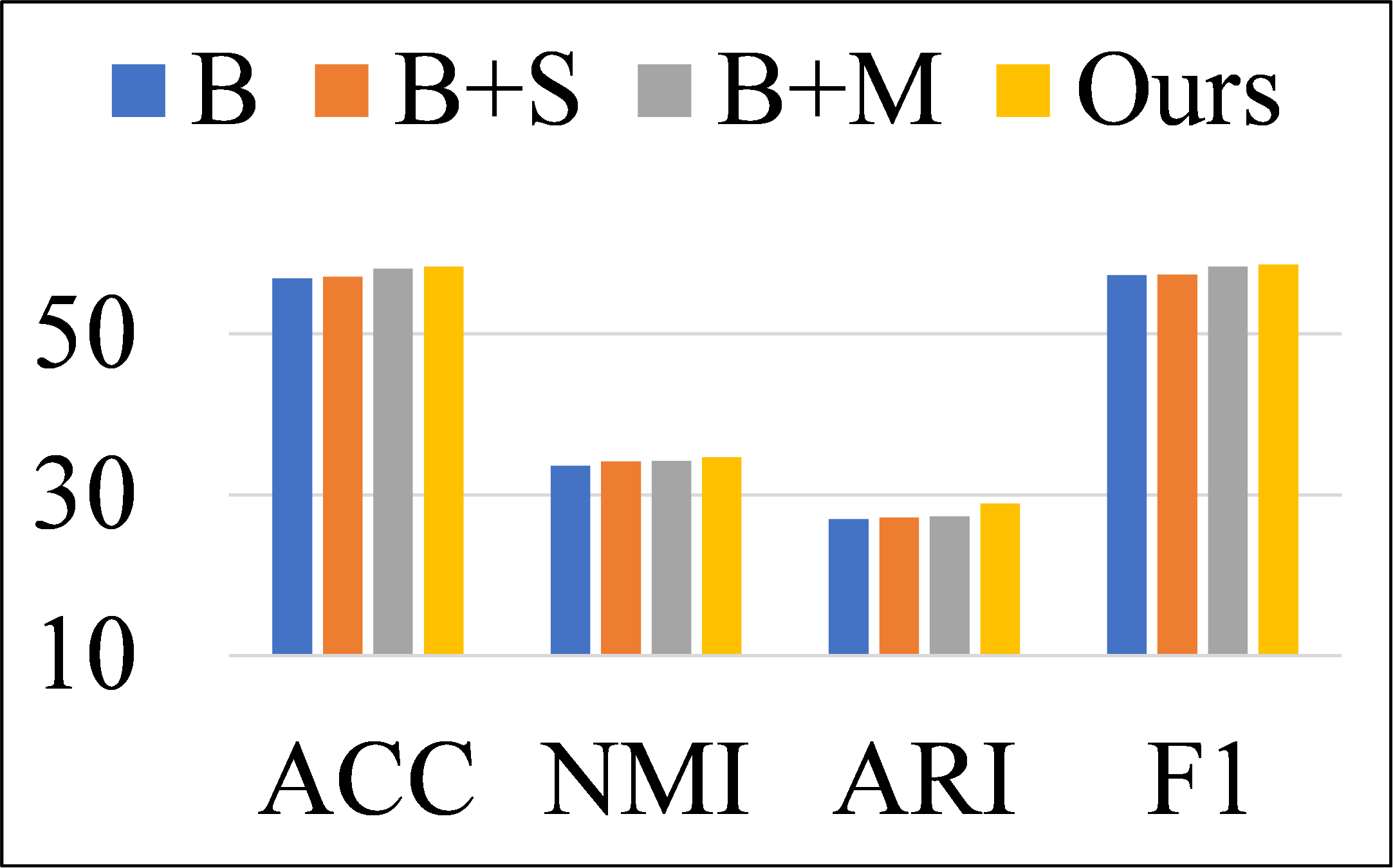
(c) EAT

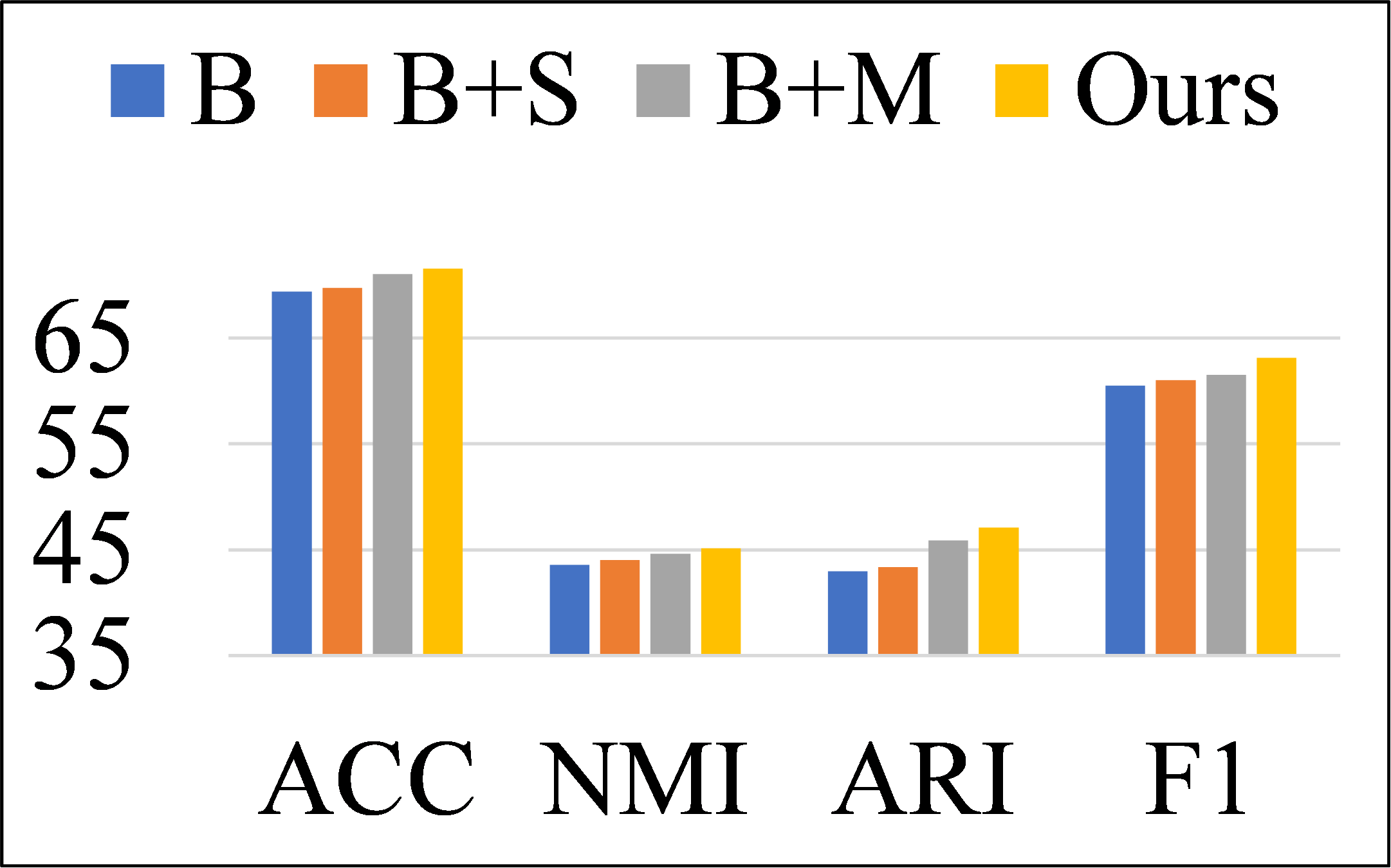
(d) CITE

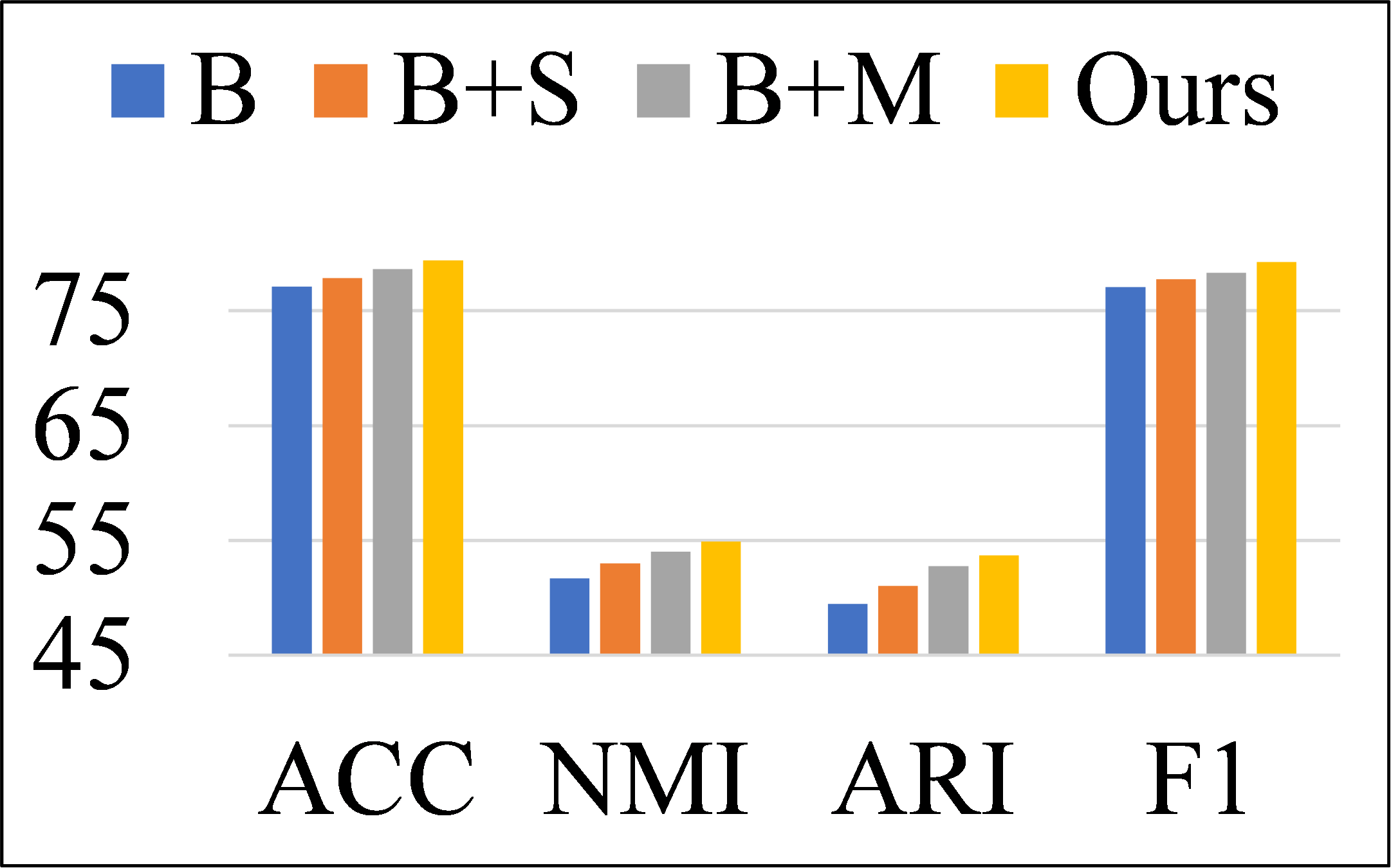
(e) BAT

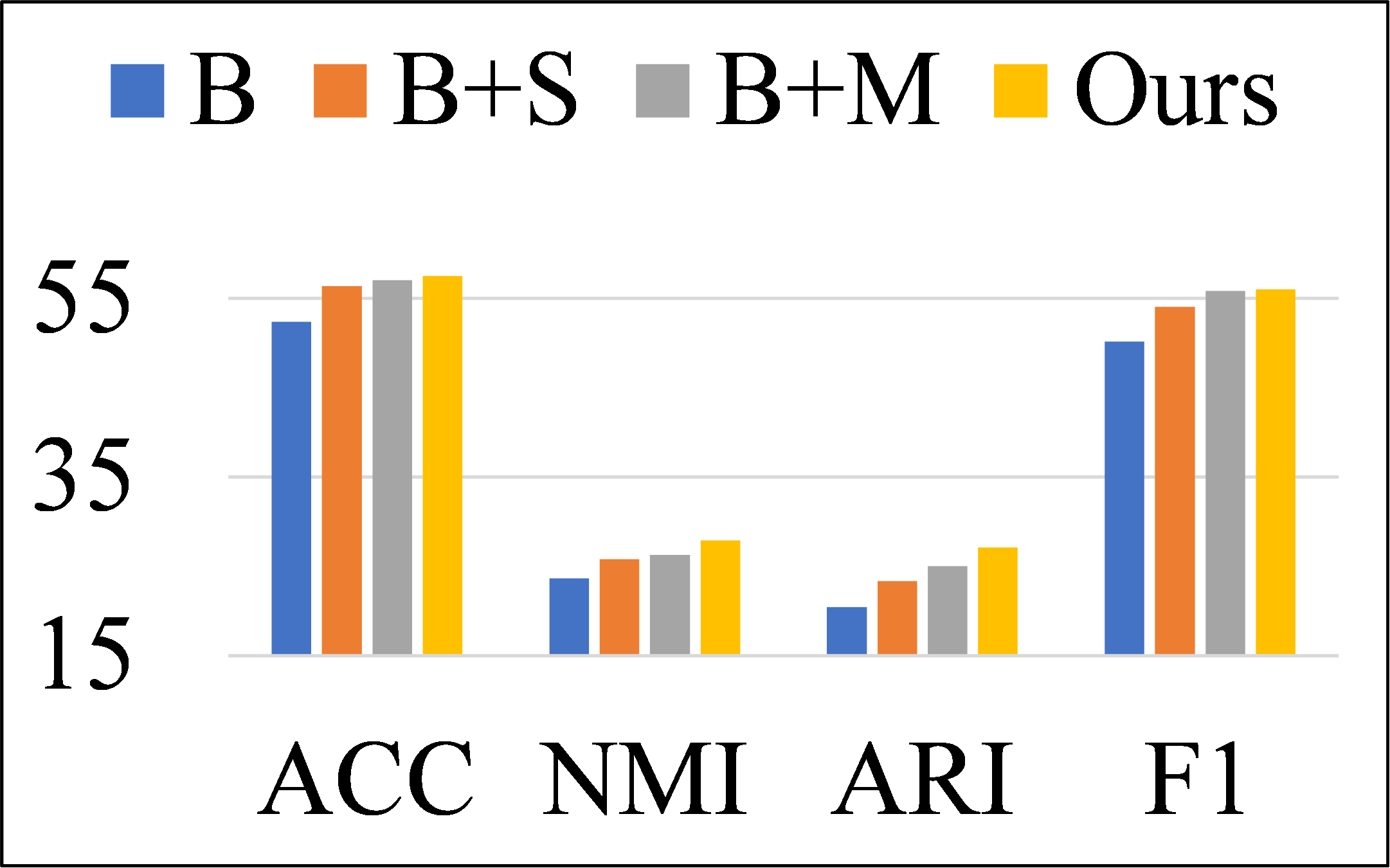
(f) UAT

Figure 4: Ablation studies of the proposed similarity function $\mathcal{S}$ and weight modulating function $\mathcal{M}$ on six datasets.

Analysis

Hyper-parameter Analysis

In this section, we analyze the hyper-parameters $\tau$ and $\beta$ in our method. For the confidence $\tau$, we select it in $\{0.1,0.3,0.5,0.7,0.9\}$. As shown in Figure 5, we observe that our method achieves promising performance when $\tau\in[0.1,0.3]$ on BAT / CITE datasets and when $\tau\in[0.7,0.9]$ on other datasets. In this paper, the confidence is set to a fixed value, thus a possible future work is to design a learnable or dynamical confidence. Besides, we analyze $\beta$ in Appendix. Two conclusions are deduced as follows. 1) The focusing factor $\beta$ controls the down-weighing rate of easy sample pairs. When $\beta$ increases, the down-weighting rate of easy sample pairs also increases and vice versa. 2) HSAN is not sensitive to $\beta$. Experimental evidence can be found in Figure 1-3 in Appendix.

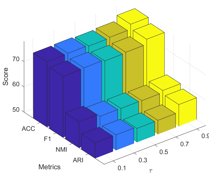
(a) CORA

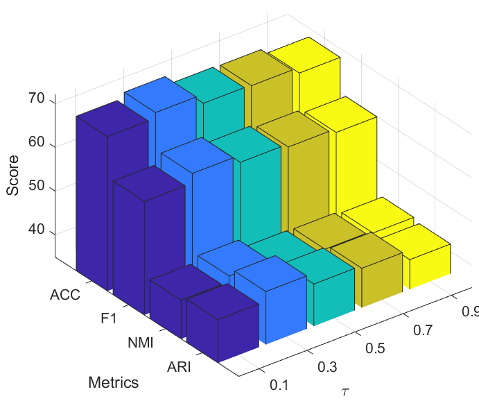
(b) CITE

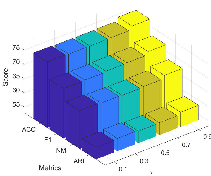
(c) AMAP

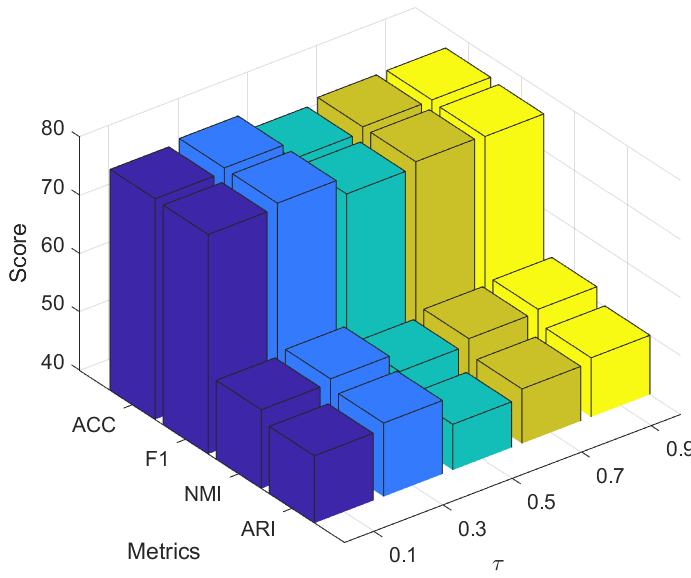
(d) BAT

(e) EAT

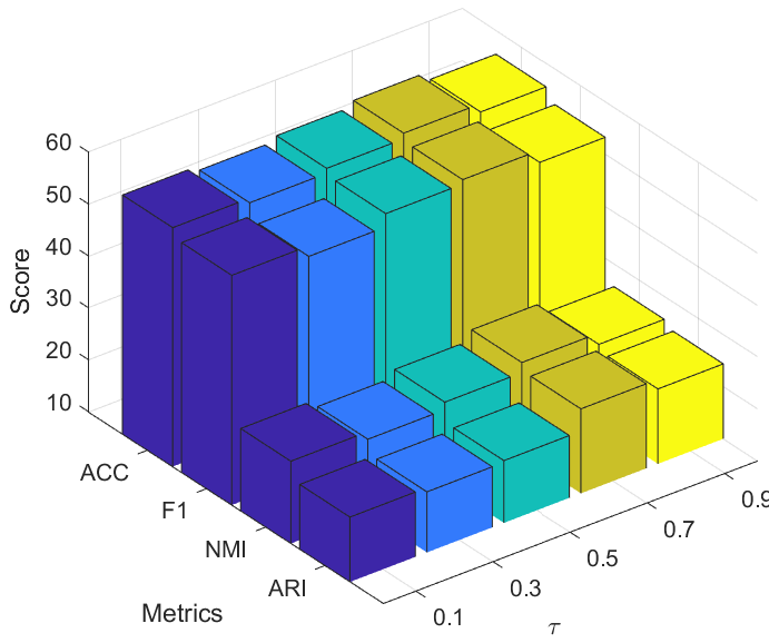
(f) UAT

Figure 5: Analysis of the confidence hyper-parameter $\tau$.

Visualization Analysis

To further demonstrate the superiority of HSAN intuitively, we conduct 2D $t$-SNE (Van der Maaten and Hinton 2008) on the learned node embeddings in Figure 3. It is observed that our HSAN can better reveal the cluster structure compared with other baselines.

Convergence Analysis

In addition, we analyze the convergence of our proposed loss. Specifically, we plot the trend of loss and the clustering ACC of our method in Figure 6. Here, “Ours” and “infoNCE” denotes our method with our hard sample aware contrastive loss, and the infoNCE loss, respectively. We observe 1) the loss and ACC gradually converge after 350 epochs. 2) after 50 epochs, “Ours” calculates the larger loss value while achieving better performance compared with “infoNCE”. The reason is that our loss down-weights the easy sample pairs while up-weighting the hard sample pairs, thus increasing the loss value. Meanwhile, the proposed loss guides the network to focus on the hard sample pairs, leading to better performance.

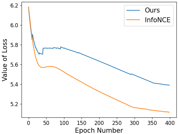
(a) Loss on BAT

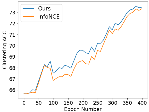
(b) ACC on BAT

Figure 6: Convergence analysis on BAT dataset.

Conclusion

In this paper, we propose a Hard Sample Aware Network (HSAN) to mine the hard samples in contrastive deep graph clustering. Concretely, we first design the attribute and structure encoders to embed the attribute and structure of samples into the latent space. Then a comprehensive similarity measure criterion is proposed to calculate the sample similarities by considering both attribute and structure information, thus better revealing the potential sample relations. Furthermore, guided by the high-confidence clustering information, we propose a general dynamic weight modulating function to up-weight the hard sample pairs while down-weighting the negative ones. In this manner, the proposed hard sample aware contrastive loss forces the network to focus on both positive and negative sample pairs, thus further improving the discriminative capability. The time and space analysis of the proposed loss demonstrate that it will not bring large time or space costs compared with the classical infoNCE loss. Experiments demonstrate the effectiveness and superiority of our proposed method. In this work, the confidence parameter is set to a fixed value, thus one future work is to design a learnable or adaptive confidence parameter.

References

- Bo et al. (2020) Bo, D.; Wang, X.; Shi, C.; Zhu, M.; Lu, E.; and Cui, P. 2020. Structural deep clustering network. In Proc. of WWW.
- Chen et al. (2022a) Chen, M.; Liu, T.; Wang, C.; Huang, D.; and Lai, J. 2022a. Adaptively-weighted Integral Space for Fast Multiview Clustering. In Proc. of ACM MM.
- Chen et al. (2022b) Chen, M.; Wang, C.; Huang, D.; Lai, J.; and Yu, P. S. 2022b. Efficient Orthogonal Multi-view Subspace Clustering. In Proc. of KDD.
- Chu et al. (2021) Chu, G.; Wang, X.; Shi, C.; and Jiang, X. 2021. CuCo: Graph Representation with Curriculum Contrastive Learning. In Proc. of IJCAI.
- Chuang et al. (2020) Chuang, C.-Y.; Robinson, J.; Lin, Y.-C.; Torralba, A.; and Jegelka, S. 2020. Debiased contrastive learning. Proc. of NeurIPS.
- Cui et al. (2020) Cui, G.; Zhou, J.; Yang, C.; and Liu, Z. 2020. Adaptive graph encoder for attributed graph embedding. In Proc. of KDD.
- Duan et al. (2022) Duan, J.; Wang, S.; Liu, X.; Zhou, H.; Hu, J.; and Jin, H. 2022. GADMSL: Graph Anomaly Detection on Attributed Networks via Multi-scale Substructure Learning. arXiv preprint arXiv:2211.15255.
- Gao et al. (2022) Gao, Z.; Tan, C.; Li, S.; et al. 2022. AlphaDesign: A graph protein design method and benchmark on AlphaFoldDB. arXiv preprint arXiv:2202.01079.
- Gong et al. (2022) Gong, L.; Zhou, S.; Liu, X.; and Tu, W. 2022. Attributed Graph Clustering with Dual Redundancy Reduction. In Proc. of IJCAI.
- Hassani and Khasahmadi (2020) Hassani, K.; and Khasahmadi, A. H. 2020. Contrastive multi-view representation learning on graphs. In Proc. of ICML.
- Hjelm et al. (2018) Hjelm, R. D.; Fedorov, A.; Lavoie-Marchildon, S.; Grewal, K.; Bachman, P.; Trischler, A.; and Bengio, Y. 2018. Learning deep representations by mutual information estimation and maximization. In Proc. of ICLR.
- Jin et al. (2021) Jin, W.; Liu, X.; Zhao, X.; Ma, Y.; Shah, N.; and Tang, J. 2021. Automated Self-Supervised Learning for Graphs. In Proc. of ICLR.
- Kalantidis et al. (2020) Kalantidis, Y.; Sariyildiz, M. B.; Pion, N.; Weinzaepfel, P.; and Larlus, D. 2020. Hard negative mixing for contrastive learning. Proc. of NeurIPS.
- Kipf and Welling (2017) Kipf, T. N.; and Welling, M. 2017. Semi-supervised classification with graph convolutional networks. In Proc. of ICLR.
- Lee, Lee, and Park (2021) Lee, N.; Lee, J.; and Park, C. 2021. Augmentation-Free Self-Supervised Learning on Graphs. arXiv preprint arXiv:2112.02472.
- Li et al. (2022) Li, L.; Wang, S.; Liu, X.; Zhu, E.; Shen, L.; Li, K.; and Li, K. 2022. Local Sample-Weighted Multiple Kernel Clustering With Consensus Discriminative Graph. IEEE Transactions on Neural Networks and Learning Systems.
- Liang et al. (2022a) Liang, K.; Liu, Y.; Zhou, S.; Liu, X.; and Tu, W. 2022a. Relational Symmetry based Knowledge Graph Contrastive Learning. arXiv preprint arXiv:2211.10738.
- Liang et al. (2022b) Liang, K.; Meng, L.; Liu, M.; Liu, Y.; Tu, W.; Wang, S.; Zhou, S.; Liu, X.; and Sun, F. 2022b. Reasoning over Different Types of Knowledge Graphs: Static, Temporal and Multi-Modal. arXiv preprint arXiv:2212.05767.
- Liu et al. (2022a) Liu, M.; Quan, Z.-W.; Wu, J.-M.; Liu, Y.; and Han, M. 2022a. Embedding temporal networks inductively via mining neighborhood and community influences. Applied Intelligence.
- Liu et al. (2022b) Liu, S.; Wang, S.; Zhang, P.; Xu, K.; Liu, X.; Zhang, C.; and Gao, F. 2022b. Efficient one-pass multi-view subspace clustering with consensus anchors. In Proc. of AAAI.
- Liu et al. (2022c) Liu, Y.; Tu, W.; Zhou, S.; Liu, X.; Song, L.; Yang, X.; and Zhu, E. 2022c. Deep Graph Clustering via Dual Correlation Reduction. In Proc. of AAAI.
- Liu et al. (2022d) Liu, Y.; Xia, J.; Zhou, S.; Wang, S.; Guo, X.; Yang, X.; Liang, K.; Tu, W.; Li, Z. S.; and Liu, X. 2022d. A Survey of Deep Graph Clustering: Taxonomy, Challenge, and Application. arXiv preprint arXiv:2211.12875.
- Liu et al. (2022e) Liu, Y.; Yang, X.; Zhou, S.; and Liu, X. 2022e. Simple Contrastive Graph Clustering. arXiv preprint arXiv:2205.07865.
- Liu et al. (2022f) Liu, Y.; Zhou, S.; Liu, X.; Tu, W.; and Yang, X. 2022f. Improved Dual Correlation Reduction Network. arXiv preprint arXiv:2202.12533.
- Meng Liu (2021) Meng Liu, Y. L. 2021. Inductive representation learning in temporal networks via mining neighborhood and community influences. In Proc. of SIGIR.
- Meng Liu (2022) Meng Liu, Y. L., Jiaming Wu. 2022. Embedding Global and Local Influences for Dynamic Graphs. In Proc. of CIKM.
- Mrabah et al. (2022) Mrabah, N.; Bouguessa, M.; Touati, M. F.; and Ksantini, R. 2022. Rethinking graph auto-encoder models for attributed graph clustering. IEEE Transactions on Knowledge and Data Engineering.
- Pan et al. (2019) Pan, S.; Hu, R.; Fung, S.-f.; Long, G.; Jiang, J.; and Zhang, C. 2019. Learning graph embedding with adversarial training methods. IEEE transactions on cybernetics.
- Robinson et al. (2020) Robinson, J.; Chuang, C.-Y.; Sra, S.; and Jegelka, S. 2020. Contrastive learning with hard negative samples. arXiv preprint arXiv:2010.04592.
- Sun et al. (2021) Sun, M.; Zhang, P.; Wang, S.; Zhou, S.; Tu, W.; Liu, X.; Zhu, E.; and Wang, C. 2021. Scalable multi-view subspace clustering with unified anchors. In Proc. of ACM MM.
- Tan et al. (2022) Tan, C.; Gao, Z.; Xia, J.; and Li, S. Z. 2022. Generative De Novo Protein Design with Global Context. arXiv preprint arXiv:2204.10673.
- Tu et al. (2020) Tu, W.; Zhou, S.; Liu, X.; Guo, X.; Cai, Z.; Cheng, J.; et al. 2020. Deep Fusion Clustering Network. arXiv preprint arXiv:2012.09600.
- Van den Oord et al. (2018) Van den Oord, A.; Li, Y.; Vinyals, O.; et al. 2018. Representation learning with contrastive predictive coding. arXiv preprint arXiv:1807.03748.
- Van der Maaten and Hinton (2008) Van der Maaten, L.; and Hinton, G. 2008. Visualizing data using t-SNE. Journal of machine learning research.
- Wan et al. (2022) Wan, X.; Liu, J.; Liang, W.; Liu, X.; Wen, Y.; and Zhu, E. 2022. Continual Multi-View Clustering. In Proc. of ACM MM.
- Wang et al. (2019) Wang, C.; Pan, S.; Hu, R.; Long, G.; Jiang, J.; and Zhang, C. 2019. Attributed graph clustering: A deep attentional embedding approach. arXiv preprint arXiv:1906.06532.
- Wang et al. (2017) Wang, C.; Pan, S.; Long, G.; Zhu, X.; and Jiang, J. 2017. Mgae: Marginalized graph autoencoder for graph clustering. In Proceedings of the 2017 ACM on Conference on Information and Knowledge Management.
- Wang and Chen (2021) Wang, L.; and Chen, L. 2021. FTSO: Effective NAS via First Topology Second Operator.
- Wang et al. (2022a) Wang, L.; Gong, Y.; Ma, X.; Wang, Q.; Zhou, K.; and Chen, L. 2022a. IS-MVSNet: Importance Sampling-Based MVSNet. In Proc. of ECCV.
- Wang et al. (2023) Wang, L.; Gong, Y.; Wang, Q.; Zhou, K.; and Chen, L. 2023. Flora: dual-Frequency LOss-compensated ReAl-time monocular 3D video reconstruction. In Proc. of AAAI.
- Wang et al. (2021a) Wang, S.; Liu, X.; Liu, L.; Zhou, S.; and Zhu, E. 2021a. Late fusion multiple kernel clustering with proxy graph refinement. IEEE Transactions on Neural Networks and Learning Systems.
- Wang et al. (2022b) Wang, S.; Liu, X.; Liu, S.; Jin, J.; Tu, W.; Zhu, X.; and Zhu, E. 2022b. Align then Fusion: Generalized Large-scale Multi-view Clustering with Anchor Matching Correspondences. arXiv preprint arXiv:2205.15075.
- Wang et al. (2021b) Wang, Y.; Wang, W.; Liang, Y.; Cai, Y.; and Hooi, B. 2021b. Mixup for node and graph classification. In Proc. of WWW.
- Wang et al. (2020) Wang, Y.; Wang, W.; Liang, Y.; Cai, Y.; Liu, J.; and Hooi, B. 2020. Nodeaug: Semi-supervised node classification with data augmentation. In Proc. of KDD.
- Wu et al. (2021a) Wu, L.; Lin, H.; Gao, Z.; Tan, C.; Li, S.; et al. 2021a. GraphMixup: Improving Class-Imbalanced Node Classification on Graphs by Self-supervised Context Prediction. arXiv preprint arXiv:2106.11133.
- Wu et al. (2021b) Wu, L.; Lin, H.; Tan, C.; Gao, Z.; and Li, S. Z. 2021b. Self-supervised learning on graphs: Contrastive, generative, or predictive. IEEE Transactions on Knowledge and Data Engineering.
- Wu et al. (2022) Wu, L.; Lin, H.; Xia, J.; Tan, C.; and Li, S. Z. 2022. Multi-level disentanglement graph neural network. Neural Computing and Applications.
- Xia et al. (2022a) Xia, J.; Wu, L.; Wang, G.; Chen, J.; and Li, S. Z. 2022a. ProGCL: Rethinking Hard Negative Mining in Graph Contrastive Learning. In Proc. of ICML.
- Xia et al. (2022b) Xia, J.; Zhu, Y.; Du, Y.; Liu, Y.; and Li, S. Z. 2022b. A Systematic Survey of Molecular Pre-trained Models. arXiv preprint arXiv:2210.16484.
- Xia et al. (2022c) Xia, W.; Gao, Q.; Wang, Q.; Gao, X.; Ding, C.; and Tao, D. 2022c. Tensorized Bipartite Graph Learning for Multi-View Clustering. IEEE Transactions on Pattern Analysis and Machine Intelligence.
- Xia et al. (2022d) Xia, W.; Wang, Q.; Gao, Q.; Yang, M.; and Gao, X. 2022d. Self-consistent Contrastive Attributed Graph Clustering with Pseudo-label Prompt. IEEE Transactions on Multimedia.
- Xia et al. (2022e) Xia, W.; Wang, Q.; Gao, Q.; Zhang, X.; and Gao, X. 2022e. Self-Supervised Graph Convolutional Network for Multi-View Clustering. IEEE Trans. Multim.
- Xie et al. (2022) Xie, F.; Zhang, Z.; Li, L.; Zhou, B.; and Tan, Y. 2022. EpiGNN: Exploring Spatial Transmission with Graph Neural Network for Regional Epidemic Forecasting. In Proc. of ECML.
- Xu and Lang (2020) Xu, Y.; and Lang, H. 2020. Distribution shift metric learning for fine-grained ship classification in SAR images. IEEE Journal of Selected Topics in Applied Earth Observations and Remote Sensing.
- Yang et al. (2022a) Yang, X.; Liu, Y.; Zhou, S.; Liu, X.; and Zhu, E. 2022a. Mixed Graph Contrastive Network for Semi-Supervised Node Classification. arXiv preprint arXiv:2206.02796.
- Yang et al. (2022b) Yang, Y.; Guan, Z.; Wang, Z.; Zhao, W.; Xu, C.; Lu, W.; and Huang, J. 2022b. Self-supervised Heterogeneous Graph Pre-training Based on Structural Clustering. arXiv preprint arXiv:2210.10462.
- Zeng et al. (2023) Zeng, D.; Liu, W.; Chen, W.; Zhou, L.; Zhang, M.; and Qu, H. 2023. Substructure Aware Graph Neural Networks. In Proc. of AAAI.
- Zeng et al. (2022) Zeng, D.; Zhou, L.; Liu, W.; Qu, H.; and Chen, W. 2022. A Simple Graph Neural Network via Layer Sniffer. In Proc. of ICASSP.
- Zhang et al. (2022a) Zhang, J.; Li, L.; Wang, S.; Liu, J.; Liu, Y.; Liu, X.; and Zhu, E. 2022a. Multiple Kernel Clustering with Dual Noise Minimization. In Proc. of ACM MM.
- Zhang et al. (2020) Zhang, P.; Liu, X.; Xiong, J.; Zhou, S.; Zhao, W.; Zhu, E.; and Cai, Z. 2020. Consensus one-step multi-view subspace clustering. IEEE Transactions on Knowledge and Data Engineering.
- Zhang et al. (2021) Zhang, T.; Liu, X.; Gong, L.; Wang, S.; Niu, X.; and Shen, L. 2021. Late Fusion Multiple Kernel Clustering with Local Kernel Alignment Maximization. IEEE Transactions on Multimedia.
- Zhang et al. (2022b) Zhang, T.; Liu, X.; Zhu, E.; Zhou, S.; and Dong, Z. 2022b. Efficient Anchor Learning-based Multi-view Clustering–A Late Fusion Method. In Proc. of ACM MM.
- Zhao et al. (2021) Zhao, H.; Yang, X.; Wang, Z.; Yang, E.; and Deng, C. 2021. Graph debiased contrastive learning with joint representation clustering. In Proc. of IJCAI.
- Zhou et al. (2019) Zhou, S.; Liu, X.; Li, M.; Zhu, E.; Liu, L.; Zhang, C.; and Yin, J. 2019. Multiple kernel clustering with neighbor-kernel subspace segmentation. IEEE transactions on neural networks and learning systems.
- Zhou et al. (2020) Zhou, S.; Nie, D.; Adeli, E.; Yin, J.; Lian, J.; and Shen, D. 2020. High-Resolution Encoder–Decoder Networks for Low-Contrast Medical Image Segmentation. IEEE Transactions on Image Processing.
- Zhu et al. (2022) Zhu, Y.; Xu, Y.; Cui, H.; Yang, C.; Liu, Q.; and Wu, S. 2022. Structure-enhanced heterogeneous graph contrastive learning. In Proc. of SDM.
- Zhu et al. (2020) Zhu, Y.; Xu, Y.; Yu, F.; Liu, Q.; Wu, S.; and Wang, L. 2020. Deep Graph Contrastive Representation Learning. In ICML Workshop on Graph Representation Learning and Beyond.