Wide-scale Monitoring of Satellite Lifetimes: Pitfalls and a Benchmark Dataset

Abstract

An important task within the broader goal of Space Situational Awareness (SSA) is to observe changes in the orbits of satellites, where the data spans thousands of objects over long time scales (decades). The Two-Line Element (TLE) data provided by the North American Aerospace Defense Command is the most comprehensive and widely-available dataset cataloguing the orbits of satellites. This makes it a highly-attractive data source on which to perform this observation. However, when attempting to infer changes in satellite behaviour from TLE data, there are a number of potential pitfalls. These mostly relate to specific features of the TLE data which are not always clearly documented in the data sources or popular software packages for manipulating them. These quirks produce a particularly hazardous data type for researchers from adjacent disciplines (such as anomaly detection or machine learning). We highlight these features of TLE data and the resulting pitfalls in order to save future researchers from being trapped. A seperate, significant, issue is that existing contributions to manoeuvre detection from TLE data evaluate their algorithms on different satellites, making comparison between these methods difficult. Moreover, the ground-truth in these datasets is often poor quality, sometimes being based on subjective human assessment. We therefore release and describe in-depth an open, curated, benchmark dataset containing TLE data for 15 satellites alongside high-quality ground-truth manoeuvre timestamps.

1 Introduction

The ability to recover the manoeuvre history of satellites is important for the analysis of their lifetimes. In particular, it is of significant interest to know whether a satellite has already reached its end of life and if its last manoeuvre has been performed in accordance with the Inter-Agency Space Debris Coordination Committee (IADC) mitigation guidelines [19], or to quickly discover unplanned manoeuvres.

Large-scale and long-term historical datasets are essential for inferring satellite manoeuvres in the post-mission mode. Detailed tracking measurements, such as optical and radar data, are not publicly available for most satellites, but the Two-Line Element (TLE) data [1] provided by the North American Aerospace Defense Command (NORAD) does provide long-term data detailing the orbits of a large number of satellites. The TLE data contains perturbation mean orbital elements, calculated by least squares from tracking observations of a space object [43, 41] and sampled at roughly daily intervals (more detail on sampling will follow). A more accurate catalogue, known as the Special Perturbation (SP) catalogue, is maintained by the $18^{th}$ Space Control Squadron and contains the sensing data of the United States Space Surveillance Network (SSN)[3]. TLEs are increasingly an outcome of fitting satellite ephemeris in the SP catalogue [27]. TLE data is publicly available from the U.S. Space Command’s space object catalog via Space-Track or Celestrak.

Most active satellites perform routine manoeuvres to change their orbital altitude or plane. A planned satellite manoeuvre is performed using the satellite’s propulsion subsystem to fire thrusters and bring about a change in its orbital elements, which otherwise would remain constant. Simple time series analysis on these orbital elements can therefore be employed to detect satellite manoeuvres. These can be enhanced by screening on TLE prediction residuals using a physical model to predict the future motion of the satellite. In particular TLE data is intended to be used in conjunction with the SGP4/SDP4 model [15], which can perform such predictions.

As explained in depth in Section 3, this model allows one to derive satellite positions across multiple time points from a single TLE. However, in this work we show that, if one’s goal is to detect changes in a satellite’s orbit over longer time periods (days or weeks), then the use of this model can be counter-productive. Specifically, in Section 4.1 and Section 4.3, we show that using the full SGP4/SDP4 model to propagate to subsequent epochs and make comparisons against the associated TLEs is not necessarily better than performing the simpler propagation of the mean orbital elements. In Section 4.2, we demonstrate how using SGP4/SDP4 to add in non-Keplerian orbit components before performing further analysis can transform the data in unexpected ways. Thus, one contribution of this work is to clarify the use of TLE data in conjunction with satellite models for change detection. That might seem minor, but we identify many past papers whose results might be more convincing with a better command of these important details.

This contribution can be summarised in three specific recommendations:

1. If possible, avoid propagating TLEs using the full SGP4/SDP4 model. Section 4.1 shows how using this model in its entirety introduces substantial noise in the propagation residuals, as compared with propagating mean elements.

2. Avoid transforming TLEs to osculating elements or satellite positions using SGP4/SDP4. If this is done, ensure that a sufficiently high sampling rate is used. Section 4.2 demonstrates how a low sampling rate can lead to aliasing of the high-frequency non-Keplerian components introduced by SGP4/SDP4.

3. If one does propagate TLEs using the full SGP4/SDP4 model, then ensure that TLEs in subsequent epochs are also transformed into osculating elements or satellite positions using this model. Section 4.3 shows the problems that can arise if this step is not included.

The second major contribution of this work is a dataset on which to base accurate results for future detection projects. Much of the previous work on detecting changes in satellite orbits from TLE data (see Section 2 for a review) has tested techniques on only a limited number of satellites. Moreover, each work chooses different satellites on which to test, and the “ground-truth” used is sometimes not a true ground truth as it is obtained from inspection of the same data being used to perform detection. In order to address these concerns, Section 5 presents an open, curated dataset of satellite TLEs and associated manoeuvre timestamps to serve as a benchmark for future work on satellite lifetime surveillance. This dataset can be found at github.com/dpshorten/TLE_observation_benchmark_dataset.

2 Previous Work

Change detection in satellite data now forms a small cottage industry, which we shall summarise below, but some definitions are needed first: each element of TLE data consists of two lines of data including an associated timestamp, which is referred to as its epoch [17], and the satellites orbital elements. The epoch is the notional time at which the data is recorded, though in fact the element may summarise a fit to data from a wider time interval. In general, we use the term epoch to mean a distinct point in time at which we can measure or predict a satellite position.

A popular approach to detecting changes in the orbits of satellites from TLE data is to propagate the TLE published for one or more epochs to the epoch associated with another TLE and compare the propagated (or predicted) and measured values [21, 22, 11, 26, 47]. The propagation should be performed using the SGP4/SDP4 model [15, 17, 41, 43] (see Section 3 for a detailed explanation of the relationship between TLE data and the SGP4/SDP4 model). Some work [26, 47] utilising this general approach simply propagates a TLE to the subsequent epoch, whereas others [11, 20, 21, 22] propagate the TLEs from multiple epochs (both forwards and backwards in time) to a given epoch before making a comparison. As will be described in detail in Section 4.3, great care must be taken to ensure that the TLE published at the epoch to which the other epochs are being propagated is also transformed using SGP4/SDP4 in order to have the non-Keplerian components of the orbit included. Much of the literature [22, 26, 21, 47] does not make it clear whether or not this step is performed. However, in some studies [26, 47], the large differences between the propagated orbital elements and those at subsequent epochs imply that it is likely that the non-Keplerian terms are not being added at the subsequent epochs.

There is also a substantial body of work which looks for changes in the TLE data using a data-centric approach, that is, without taking into account the underlying orbital dynamics [39, 4, 16, 28, 40, 38, 10, 18, 33, 44, 45]. The dominant data-centric approach uses some method to predict the values in a TLE based usually on past TLE values, but sometimes also including future TLEs in the predictions. If the recorded TLE deviates substantially from the predictions, then this is taken to be indicative of some change in the satellite’s orbit. The simplest such approach is that published by Songet al.[39], who applied outlier detection methods to changes in the semi-major axis between subsequent epochs. A number of studies applied polynomial regression to the prediction of TLE updates [4, 16, 28, 40]. Shivshankar and Ghose [38] apply classic time-series forecasting techniques to this problem. Two studies [10, 18] used neural networks to predict TLE values.

An alternative data-centric approach focuses specifically on the problem of detecting the timestamps of satellite manoeuvres and solves this task using supervised machine learning [44, 45]. That is, these studies compile datasets of TLE data and associated ground-truth manoeuvre timestamps and train models on this combination in order to be able to predict the presence of manoeuvres in unseen data. The study by Wanget al.[45] is unusual here, as, unlike other studies which make use of TLEs published by NORAD [17], they only make use of simulated data.

While the above-mentioned data-centric approaches operated on the raw TLE values (or a simple transformation of them, such as transforming the mean motion to the semi-major axis), Roberts and Linares [33] first created a regularly-sampled time series by propagating the TLEs using SGP4/SDP4 to sample points. A convolutional neural network is trained on a set of this data for which labelled manouevre timestamps are also provided.

An interesting counterpoint to these studies using supervised machine learning is the work of Shabarekhet al.[36, 37], who present machine learning approaches for predicting satellite manoeuvre timestamps based solely on historic manoeuvre times (that is, without any TLE data).

There are two notable studies [8, 20] that develop both data-centric and propagation-based approaches and contrast the two.

Finally, there are two significant recent studies that focus on the problem of inferring manoeuvre parameters from the TLEs at the epochs on either side of a given manoeuvre. Yuet al.[46] developed a model-based approach for determining the time point of a manoeuvre based on the mean orbital elements before and after the manoeuvre. It depends on preexisting knowledge that the manoeuvre took place. Pirovano and Armellin [30], develop an optimisation framework for estimating manoeuvre parameters for an unknown manoeuvre occurring between two TLE epochs. They show how this approach can also be adapted to manoeuvre detection.

The striking factor in these studies, particularly the data-centric studies, is that TLE data is often used in a manner that does not display a clear understanding on the non-Keplerian elements of orbital dynamics, and that can cause problems as we show below. It is towards this gap that this paper and the associated dataset are aimed.

3 Description of TLE Data

TLE is a data format encoding the orbital elements of Earth-orbiting objects. The data is encoded in ASCII text files as a sequence of characters and numbers. A single element is actually encoded over three lines in the form:

ISS (ZARYA)
1 25544U 98067A   08264.51782528 -.00002182  00000-0 -11606-4 0  2927
2 25544  51.6416 247.4627 0006703 130.5360 325.0288 15.72125391563537

where the first line encodes the 24 character name of the object, and the first data line contains information about the satellite (classification, international designator, …) and the epoch (the time point to which the measurement pertains). The second data line contains the orbital elements. Both lines have an additional checksum. The data are formatted over multiple lines because the format’s original use was on 80-column punch cards.

The pitfalls that can occur when analysing TLE data stem from some misunderstandings around the nature of what this data represents. This is understandable, as certain features of this data are often not clearly documented. This lack of clear documentation can make it difficult for those from other domain areas (such as anomaly detection or machine learning) to apply their knowledge to this area. As such, we first describe in some detail what the values in TLE data do represent, with a focus on making concepts clear to researchers unfamiliar with satellite orbit data. Subsequent sections will focus on some of the pitfalls that these misunderstandings can lead to.

The main potential source of confusion around TLE data is that reported numerical values are quite far removed from the underlying physical quantities. Anomalies in the data can therefore be the result of changes in how the underlying physical quantities are being transformed, as opposed to changes in the quantities themselves. This is in contrast with, say, financial market data, where the price associated with a stock bid is closely associated with the actual stock-market behaviour. Further, the relationship between TLE data and the models for propagating it is not straightforward (see below).

In an idealised model of an orbit, we would consider a small point mass (a satellite) orbiting a substantially larger point mass (the earth). This will result in an elliptical orbit which can be described by five parameters, typically the parameterisation used is: the semi-major axis ($a$), eccentricity ($e$), inclination ($i$), longitude of the ascending node ($\Omega$) and argument of the periapsis ($\omega$). A sixth parameter, the mean anomaly ($M$), describes the point along this ellipse where the satellite sits at a given epoch. These six parameters are usually referred to as Keplerian elements [34, 42].

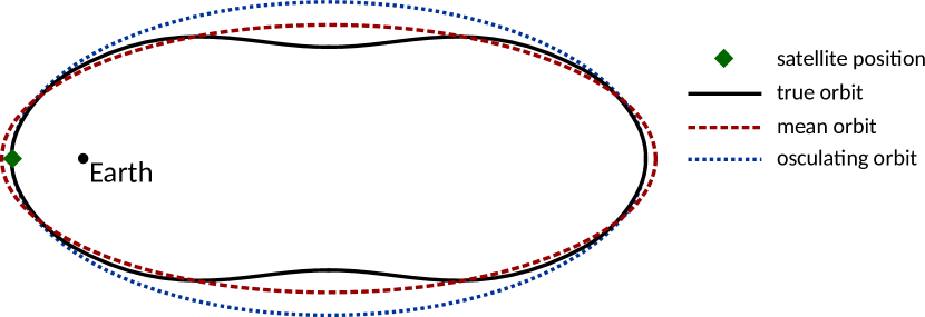
Figure 1: An illustration of mean and osculating orbits. The figure shows a satellite and its true orbit (which is non-elliptical due to perturbations), the mean (elliptical) orbit best fitting its overall path, and the osculating (elliptical) orbit for the satellite at perigee. Note that all affects are strongly exaggerated to make the illustrated differences more obvious. In particular one can see that using the mean orbit to estimate position will only be valid on a set of measure zero, but likewise, propagating the osculating orbit will be inaccurate at any point except the one for which it is calculated.

There are other parametrisations which can describe an orbit. Notable in the current context would be the three-dimensional position and velocity vectors $\vec{x}$ and $\vec{v}$ [34, 42]. It is easy to transform these vectors into the Keplerian elements using the mass of the larger object.

Real satellites, however, do not orbit in perfect ellipses [42]. This is due to factors such as the gravitational pull of other bodies (such as the moon) and atmospheric drag. A question then arises: given that the orbit is not elliptical, if we are given position and velocity vectors, how do we transform these into Keplerian orbital elements? There are two Keplerian orbits that can be used to describe the motion of the satellite: the $mean$ and $osculating$ orbits [34, 42].

Figure 1 illustrates the two elliptical representations of an orbit, though note it is substantially exaggerated. The osculating orbit is the Keplerian orbit that “kisses” the true orbit at the point at which the satellite currently sits. That is, it is the Keplerian orbit which will most closely approximate the motion of the satellite in the small neighbourhood around its current position. By contrast, the mean orbit is the Keplerian orbit which will most closely approximate the satellite’s orbit across its entire orbital period. This distinction is important when we are transforming Keplerian orbital elements into position vectors. If we translate the mean Keplerian orbital elements into position and velocity vectors in the straightforward manner that we might do for an elliptical orbit [9], then these vectors might differ significantly from the actual position and velocity.

Most importantly for change detection, we note that the mean orbital elements remain approximately constant, but inaccurate, while the osculating elements are accurate, but depend on the satellite location, so they vary periodically.

TLE data contains the mean Keplerian orbital elements (apart from the semi-major axis, although this can easily be recovered from the mean motion) [15, 41]. TLE data is intended to be used in conjunction with the SGP4/SDP4 orbital propagator. Although it is often referred to as a ‘propagator’, the purpose of SGP4 is not only to propagate orbits to later points in time, but also to recover the osculating orbit (and precise satellite positions and velocities) from the mean orbit [15, 41, 47]. Doing so also requires the satellite’s ballistic drag coefficient, which is provided in the TLE data. The implication of this is that the orbital elements contained in the TLE data can give a poor estimation of the current position and velocity of the satellite. It is only when the non-Keplerian components of the orbit are reintroduced via the SGP4/SDP4 model that we arrive at a reliable estimation of the satellite’s current state.

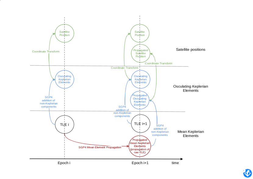
Figure 2: The process by which a TLE record can be used and propagated to a subsequent epoch. The goal of propagation is often to compare the propagated values to measured values at a subsequent epoch. There are a number of ways that this comparison can be done. One could compare the mean Keplerian elements propagated by SGP4/SDP4 with the mean orbital elements in the TLE recorded at the subsequent epoch. Alternatively, one could use SGP4/SDP4 to incorporate the non-Keplerian components of the orbit in order to generate a precise position for the satellite at the instant of the TLE epoch. This could be expressed as either osculating Keplerian elements or as position and velocity vectors.

Popular software libraries for manipulating TLE data (such as Skyfield [32] and pyorbital [14]) obscure some of these details for ease of use. These libraries make it easy to load TLE data and then query satellite positions or orbital elements. However, if we query the orbital elements or satellite positions at the same time point as a given TLE epoch, we will not be returned the original orbital elements of the TLE or a simple conversion from these elements to positions. Rather, the SGP4/SDP4 model is used to incorporate the non-Keplerian terms not present in the TLE data before returning any values to the user.

We need to take great care in how we treat orbital elements or positions to which these non-Keplerian components have been added. Some of these non-Keplerian components have periods much shorter than the interval between published TLE datapoints. This means that these components can be highly aliased [23]. Moreover, NORAD can and does make changes in the relative timepoints at which TLEs are published, which will change the effect of this aliasing. This phenomenon is demonstrated on a real satellite in Section 4.2.

The SGP4/SDP4 model first propagates the mean orbital elements, before the non-Keplerian terms are incorporated (see page 12 of [15]). It is possible to use this first component separately to model the evolution of the mean elements. Indeed, the very popular python-sgp4 library [31] (used by Skyfield) offers this functionality. Figure 2 provides a diagram showing the various modifications that can be made to TLEs, particularly within the context of comparing the propagation of one TLE to the TLE at the subsequent epoch. There are two ways of doing this. We could propagate the first TLE to the subsequent epoch using the full SGP4/SDP4 model. We would then also need to add the non-Keplerian terms to the TLE at the subsequent epoch with SGP4/SDP4. We could then compare the resulting osculating orbital elements or satellite positions. An alternative approach would be to just propagate the mean elements from the first TLE and compare these propagated elements directly against the values recorded in the subsequent TLE. Section 4.1 contrasts these two approaches in more depth. It is shown that the use of the full SGP4/SDP4 model can be detrimental to the purpose of detecting long-term changes in satellite orbits.

4 Potential Pitfalls

In this section, we analyse three pitfalls that can be encountered when analysing TLE data for the surveillance of satellite lifetimes. The first pitfall (Section 4.1) occurs with regularity in published research [8, 11, 47, 20] and also snared the authors in preliminary research using TLE data. The second pitfall (Section 4.2) is one that the authors have personally encountered and also occurs at least once [33] in the published literature. It is difficult to confirm whether the third pitfall (Section 4.3) was encountered in a given study without inspecting the scripts used to run the analysis. However, there are studies [26, 21, 22] where the figures suggest that it might have played a role.

4.1 Pitfall 1: Including non-Keplerian Components in Propagation

This subsection makes the recommendation that, if one propagates TLEs to subsequent epochs in order to make comparisons with the TLEs recorded at those epochs, then it is preferable to only propagate the mean elements. This is as opposed to using the full SGP4/SDP4 model.

The most common approach towards detecting anomalous updates in TLE data is to propagate the TLE from a given epoch to subsequent epochs and to then compare the propagated positions with those recorded from those in subsequent epochs [8, 11, 47, 20, 26, 21, 22]. There are also more complicated variations on this theme, such as propagating over multiple epochs or propagating backwards in time, or compositions of methods into larger schemes.

To the best of the authors’ knowledge, existing research that utilises this approach performs the propagation using the full SGP4/SDP4 model, which includes the non-Keplerian components. As described in detail in Section 3, the orbital elements in the TLEs correspond to the mean orbit of the satellite, which is the Keplerian orbit which best approximates its behaviour throughout a full orbit. Finding the position vectors which correspond with these mean Keplerian elements does not make sense, as the resulting positions will correspond to points on a fictional orbit, as opposed to the actual satellite positions. The standard practice for obtaining satellite positions from TLE records is, therefore, to use the SGP4/SDP4 model to reintroduce the non-Keplerian orbital components before calculating positions [41]. Comparisons to subsequent (or past) records are then usually made based on the satellite positions. Most often, comparison is made in the radial, in-track and cross-track directions, as these correspond to the directions in which thrust is applied during manoeuvres [25]. Given that this is the standard approach, and that current software implements this approach by default, we make the assumption that in previous work when comparisons of position vectors are made, unless explicitly stated, these positions are arrived at by using the full SGP4/SDP4 model.

This subsection argues that using the full SGP4/SDP4 model for propagation [21, 22, 11, 26, 47] introduces unnecessary complexity into the analysis. The SGP4/SDP4 model first propagates the mean orbital elements, before incorporating the non-Keplerian terms (see page 12 of [15]). A simpler analysis technique propagates the mean elements to the desired epoch and then compares the propagated mean elements directly against the raw TLE elements (a straightforward transform between the mean motion and semi-major axis is required). This approach greatly reduces the complexity of the comparison process. Only one of the two TLEs needs to be modified by SGP4/SDP4. Moreover, this modification only involves a subset of the usual terms of this model.

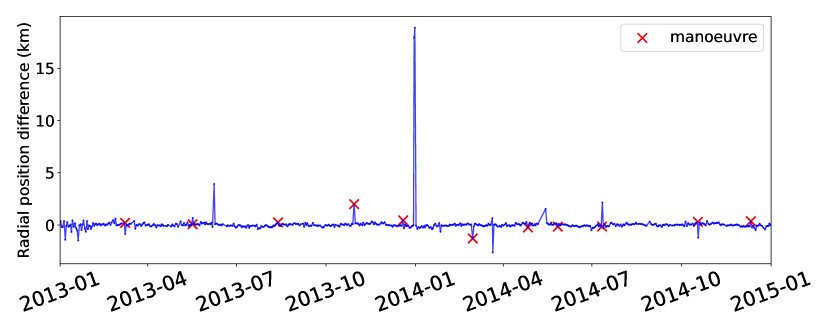
(a) Radial position difference, one epoch propagation

(b) Difference in mean semi-major axes, one epoch propagation

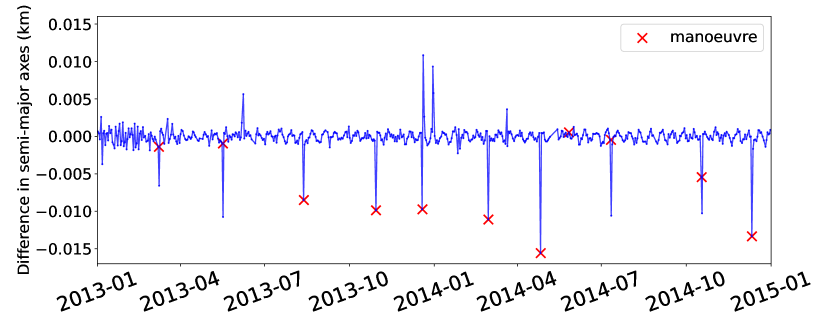
(c) Difference in osculating semi-major axes, one epoch propagation

(d) Difference in mean semi-major axes, five epoch propagation

(e) Difference in osculating semi-major axes, five epoch propagation

Figure 3: The different techniques for propagating a TLE to a subsequent epoch and then comparing the propagation to the TLE associated with that epoch for the Jason 2 satellite in the years 2013 and 2014. Independently obtained manoeuvre timestamps are shown with red crosses. Subfigure (3(a)) shows the result of performing propagation using the full SGP4/SDP4 model and then computing differences in the radial position. Note that some large propagation differences (e.g., around Jan 2014) do not align well with manoeuvre timestamps. Figure 12 in appendix B shows similar phenomena in both the in-track and cross-track directions. Subfigures (3(b)) and (3(c)) show differences between propagated and measured values for the semi-major axis. The magnitude of these differences corresponds fairly well with the manoeuvre timestamps. Subfigure (3(b)) shows the difference between propagating the mean semi-major axis and the mean semi-major axis in the subsequent TLE (obtained from the mean motion), whereas (3(c)), By contrast, propagates the semi-major axis using the full SGP4/SDP4 model and compares the propagations against the osculating element in the subsequent epoch, also obtained using SGP4/SDP4. There are small, but significant, differences in the propagation errors shown in (3(b)) and (3(c)). Subfigures (3(d)) and (3(e)) are equivalent to (3(b)) and (3(c)), but show the errors when the propagation is performed over five epochs, as opposed to one. Here the differences between propagating mean elements and using the full SGP4/SDP4 model are much starker. The propagations using the full SGP4/SDP4 model exhibit substantially larger noise in their errors. Figure 13 and Figure 14 in appendix B show similar plots to (3(b)) through (3(e)), but also include the inclination and eccentricity.

Due to the high-frequency nature of influences that affect satellite orbits, small differences in mean orbital elements can lead to substantial differences in resulting osculating orbits or calculated satellite positions. We argue that the mean elements and their propagations contain sufficient information for detecting changes in satellite orbits and that the addition of non-Keplerian components is unhelpful.

In the remainder of this subsection, we use the TLE data for the Jason-2 satellite in 2013 and 2014 as an example, with maneuver data independently obtained from the International DORIS Service (see Section 5.1 for details). We show that using the full SGP4/SDP4 model for propagation and comparison of this data is less effective than just propagating mean orbital elements. Although this does not demonstrate that this will always be the case, it suggests that care should be taken before employing SGP4/SDP4 when analysing lifetime trends in satellites.

Figure 3 shows the results of performing propagations and comparisons using the different techniques described above for the TLE data of Jason 2 from 2013 and 2014. We begin with the typical approach for detecting anomalous updates in TLE data. This technique propagates each TLE to the timestamp of the subsequent epoch using the full SGP4/SDP4 model. Non-Keplerian components are then added to the TLE at the subsequent epoch using SGP4/SDP4. 3(a) Shows the differences in the radial direction between the resulting propagated and non-propagated positions. 12(b) and 12(c) in appendix B show the same calculations in the cross-track and in-track directions, respectively. There is not a particularly close alignment between the magnitude of the errors and the manoeuvre timestamps in any of these three directions, especially when compared with the similar plots for the semi-major axis (3(b) and 3(c)).

Next, we perform similar computations, but find the differences between propagated and measured Keplerian orbital elements. This is performed both for the osculating elements, using the full SGP4/SDP4 model, as well as for the mean elements. 3(b) shows the results of propagating the mean semi-major axis and finding the difference with the semi-major axis of the TLE at the subsequent epoch (obtained from the mean motion). This can be compared with 3(c), which shows the results of the same process, but using the corresponding osculating elements. That is, the TLEs are propagated using the full SGP4/SDP4 model and the TLEs at the subsequent epoch are converted to osculating Keplerian elements using SGP4/SDP4. Although these plots are similar, there are distinct differences between them. For instance, in June 2013 there is a single very large propagation error in the osculating element propagations that is not present in the mean element propagations.

Similar plots, showing the propagation errors for both mean and osculating elements, for the inclination and eccentricity can be found in Figure 13.

Many methods for detecting anomalous updates to TLEs perform multiple propagations for each epoch, some of which will be over multiple epochs (that is, they will propagate further than the adjacent epoch) [11, 20, 21, 22]. 3(d) and 3(e) show the same plots as 3(b) and 3(c), respectively, however, the propagation is performed over five epochs. These show that performing propagations and comparisons using the full SGP4/SDP4 model introduces substantially more noise as opposed to operating solely on mean elements. Figure 14 shows plots of the propagation errors over five epochs for other orbital elements, with the same conclusion.

In summary, for the Jason-2 satellite in the years 2013 and 2014, if we want to propagate the TLEs and compare them against TLEs in subsequent epochs, then there are advantages to propagating the mean elements and comparing against the mean orbital elements recorded in the TLE for the subsequent epoch. Using the full SGP4/SDP4 model as well as calculating differences in satellite positions can introduce additional noise in the calculations and produce large deviations that do not align well with changes in the satellite’s orbit.

4.2 Pitfall 2: Sampling Osculating Orbits at Low Rates

Here we recommend that it is preferable to avoid converting TLEs to osculating orbits or satellite positions using SGP4/SDP4 before performing further analysis. Moreover, if this is done then care must be taken to use a sufficiently high sampling rate.

When analysing TLE data, especially when applying a general-purpose data analysis algorithm, it seems reasonable to convert the mean elements in the TLE data to either osculating orbital elements or positions. Mean elements are, after all, an approximation. One can use SGP4/SDP4 to produce such values either at regularly sampled intervals, or at the epoch times associated with the TLE, moreover, the most common software packages for working with TLE data do such transformations by default, to aid in ease of use.

It is then necessary to choose a method by which a sample point will be placed. One option (which is explored below) is to sample at the same time points as the published TLE epochs — resulting in a sampling rate of around once per day, but irregularly placed samples, which is inconvenient for most time-series algorithms. An alternative is to interpolate to a set of samples at regular intervals. For example, Roberts and Linares [33] sample at a fixed interval of one day. However, both such approaches inadequately sample the non-Keplerian components of satellite orbits. For instance, the variation in the semi-major axis of many satellites has a dominant frequency at twice the orbital frequency (see Appendix A). As low-earth-orbit satellites can have periods below 2 hours, The Nyquist sampling rate (that would avoid aliasing problems) is well above once per half hour in order to avoid aliasing.

The TLE data of the Jason 2 satellite contains a striking example of the potential negative consequences of analysing osculating elements with low sampling rates. The semi-major axis of the osculating orbit of Jason 2 is plotted (in blue) in 4(a), along with the semi-major axis of the mean orbit (in green). The figure includes all epochs between the 1^st of February and the 1^st of May 2013. Between the 1^st and 25^th of February, the semi-major axis of the osculating orbit appears to remain almost constant. After the 25^th of February it begins fluctuating substantially.

Observing only the semi-major axis of the osculating orbit, many reasonable observers would be tempted to conclude that some feature of the satellite’s orbit had changed on or around the 25^th of February 2013. However, we can also see that the semi-major axis of the mean orbit undergoes no substantial change and there was no published change in the orbit or mission of Jason 2 during this period.

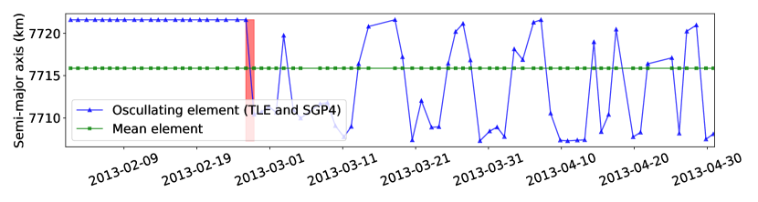
(a) Semi-major axes of the mean and osculating orbits

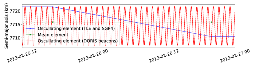
(b) High-resolution view of the highlighted part of (a)

Figure 4: A vivid demonstration of how TLE data can be confusing to work with. (4(a)) shows both the mean and osculating values for the semi-major axis of the Jason 2 satellite in early 2013. We observe that the osculating values change from being constant to varying substantially. This is strange behaviour which would probably trigger an anomaly in many anomaly detection algorithms. The causes of this strange behaviour are made clear in (4(b)), which focuses in on the onset of the fluctuating period. In this figure, more accurate data derived from DORIS ground beacons [6] is included in the plot. We can observe that, prior to the fluctuations, the timestamps associated with the TLE data aligned with the apex of the oscillations in the semi-major axis. This alignment was broken at the point the fluctuations begun.

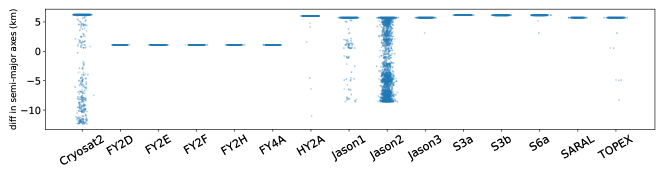
(a) Semi-major axis

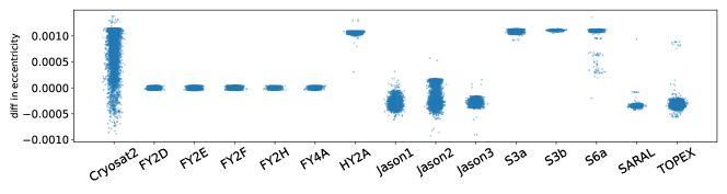
(b) Eccentricity

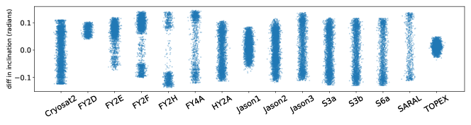
(c) Inclination

Figure 5: Rainfall plots visualising the distributions of the differences between orbital elements of the mean and the osculating orbits of the satellites included in the presented dataset. For the semi-major axis (5(a)), the majority of satellites have highly concentrated distributions. This is due to the epoch times always coinciding with the same phase in the high-frequency parts of the non-Keplerian components of the orbit. Other satellites, notably Cryosat 2, Jason 1 and Jason 2 have much broader distributions in this difference. Inspection of the semi-major axis of the osculating orbit (as show in 4(a)), shows that, in these cases, the phase within the non-Keplerian components of the orbit at which the epoch times are published varies during the period of the published data. There is a similar effect for the eccentricity (5(b)), where most satellites have a highly concentrated distribution, whereas Cryosat and the Jasons have broader concentrations. Conversely, all satellites have similarly broad distributions for the inclination (5(c)), indicating that the published epoch times are not sampling this component synchronously (that is, always at the same point within an oscillation).

The artefacts in the orbital data can be understood by inspecting the highly-accurate and finely-sampled recordings of this satellite’s semi-major axis. 4(b) contains the semi-major axis of the osculating orbit of Jason 2 as measured by ground radio beacons from the DORIS network [6]. Due to the high-frequency variation of this data, we have limited the $x$-axis to only cover the period from the 25^th to the 27^th of February (where the interesting change occurred). We see that the semi-major axis of the osculating orbit derived from the TLE data closely matches the semi-major axis of the osculating orbit derived from the DORIS beacons, both before and after the change in variation. Only two TLE data points can be shown in this plot, but this close correspondance continues to both the left and the right of the plotted region. What does change, however, is that the epoch dates published by NORAD align with the apex of the oscillations before the 25^th of February but this alignment is broken after this date. In essence, the manner in which the high-frequency parts of the non-Keplerian components are being aliased changes.

The conclusion of this analysis of Jason 2 is that, if we sample the osculating orbit at the published epoch times, we can get a very skewed view of the actual changes in the orbit of the satellite. In this example, although we observe a large change in the observed data after the 25^th of February 2013, this does not reflect any corresponding large change in the orbit of the satellite. It is merely the result of a relatively small change made by NORAD in times at which is observed the data.

Figure 5 shows the degree to which this effect is present in the historic data for the various satellites included in the benchmark dataset presented in Section 5. Rainfall plots show the distribution of the differences between the orbital elements associated with the osculating and mean orbit at each published epoch. This is done for the semi-major axis (5(a)), eccentricity (5(b)) and inclination (5(c)). Most satellites in this dataset have relatively narrow distributions of these differences for the semi-major axis and eccentricity. This is indicative of the published epoch times sampling these components synchronously. That is, they are always sampled at (close to) the same point in their phase. By contrast, CryoSat-2 and the Jason satellites have much broader distributions, which indicates changes in the phase at which this sampling takes place. However, the important point is that we have no control over exact sample times, and so these same effects could be present in any satellite’s data at some time period.

Aliasing is a well-understood phenomena in signal processing, but is perhaps so well-known that most signal processing data are automatically passed through band-pass filters before sampling. It is therefore commonly assumed that a dataset will have had aliasing effects removed before proceeding to the stage of, for instance, change detection. It is therefore a key pitfall that certain aspects of TLE data have not undergone this pre-processing.

4.3 Pitfall 3: Comparing Full SGP4 Propagations to Mean Elements

In this subsection we recommend that, if TLEs are propagated using the full SGP4/SDP4 model, then care must be taken to ensure that TLEs in subsequent epochs are also transformed with this model before comparisons are made.

There is a further trap relating to propagating TLEs. It is similar in nature to the first pitfall discussed in Section 4.1, however, it can lead to more serious consequences. This occurs when the TLEs are propagated using the full SGP4/SDP4 model, but the resulting osculating orbital elements are compared to the mean TLE elements in the subsequent epoch. That is, the non-Keplerian components of the orbit are not added to the TLE at the subsequent epoch before the comparison is made. The description of TLE data and the SGP4/SDP4 model provided in Section 3 reveals why this is problematic — it results in a comparison between fundamentally different types of orbital elements.

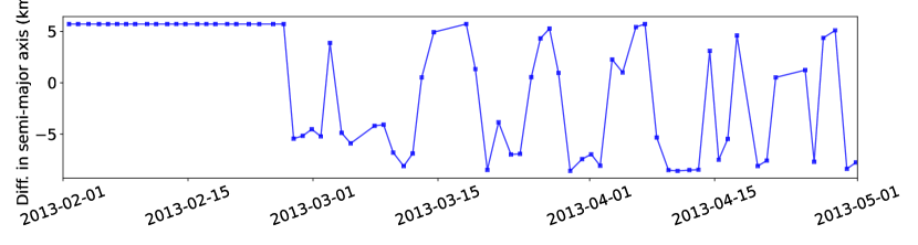
(a) Differences between the semi-major axis propagated from the previous epoch and the mean element at the current epoch.

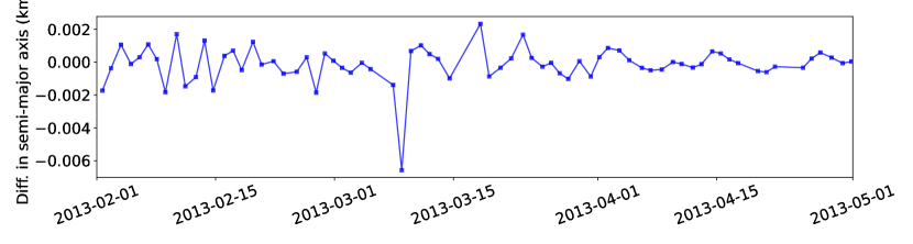
(b) Differences between the semi-major axis propagated from the previous epoch and the osculating element at the current epoch.

Figure 6: A demonstration of why it is necessary to be careful what propagated TLE elements are compared against. Both plots show the differences between the semi-major axis propagated from the previous epoch to the current epoch and that recorded at the current epoch for the Jason 2 satellite. Note that the time period covered is the same as in 4(a). Subfigure (6(a)) shows the difference with the mean element and (6(b)) shows the difference with the osculating element at the current epoch. Note the difference in the scales of the $y$ axes. Two points should stand out. The first is that the differences between the propagated element and the osculating element are substantially lower than the differences between the propagated element and the mean element. The second is that, when comparing with the mean element, the distribution of the differences goes through a dramatic change in early March of 2013. No such change is observed when comparing with the osculating element.

The consequence of this is that changes in the differences between propagated and subsequent elements might be dominated by changes in the phase at which the high-frequency parts of the non-Keplerian components are sampled, as opposed to changes in the orbit itself. An example of this is shown in Figure 6, where 6(a) shows the result of propagating the TLEs of Jason 2 using the full SGP4/SDP4 model and comparing the resulting osculating semi-major axis with the mean semi-major axis in the subsequent epoch. Note that 6(a) is plotting the same satellite over the same time period as 4(a). We observe a similar effect to the second pitfall described in Section 4.2: the residuals between the propagations and the TLEs undergo a substantial increase after the 25^th of February 2013. As in that instance, it would be tempting to conclude that there was a change in the satellite’s orbit. However, as discussed in Section 4.2, there are no published changes in the orbit or mission of Jason 2 around this time. Moreover, close inspection of accurate orbital data (see 4(b)) reveals that what has changed is that the published epoch times no longer coincide with the peaks in the oscillations of the semi-major axis. This leads to a change in the variance of the osculating semi-major axis sampled at these points, which subsequently changes the variance of the residuals. 6(b) plots the differences between the propagated semi-major axis (using the full SGP4/SDP4 model) and the osculating semi-major axis obtained from the subsequent TLE. Although this approach will suffer from the issues highlighted in Section 4.1, during analysed period it does not experience the same dramatic changes as comparing osculating and mean elements.

5 Dataset Description

There now exists a substantial body of work describing methods for analysing trends in a satellite’s orbit across its lifetime using TLE data. See Section 2 for a review of this literature. It is common, however, for each contribution to evaluate its methods on different satellites; and little attempt is therefore made to make performance comparisons with previously approaches. Evaluation is also usually performed on a relatively small set of satellites (2-5), and ground-truth data, against which performance is measured is rarely obtained from an independent source.

We present here a curated, benchmark dataset for satellite orbit surveillance using TLE data. The goal is to facilitate future studies by providing and easy-to-use dataset, that is larger than any existing set, and provides accurate ground truth for better performance evaluations and comparisons. The dataset consists of 15 diverse satellites and associated manoeuvre timestamps. It can be found at github.com/dpshorten/TLE_observation_benchmark_dataset.

The core of the curated dataset consists of the TLE data and associated independently obtained ground-truth manoeuvre timestamps. More accurate DORIS data detailing precise satellite positions (as available) is also included. This additional data is only intended to be used for the purpose of determining the accuracy of the TLE data and the associated SGP4/SDP4 propagator [1]. A list of all satellites included in the dataset is given in footnote 4, along with summary statistics of the data and features of the satellites. These satellites were chosen based on availability of the manoeuvre timestamps, as well as with the goal of providing a diversity of types of satellite, including both geostationary and low-earth-orbit satellites.

	SATCAT	TLE	Observed Manoeuvres				Altitude
Name	Number	Epochs	Num	First	Last	DORIS	(km)
Fengyun-2D	$29\,640$	$1178$	$22$	2011-02-01	2015-04-10		$35\,786$
Fengyun-2E	$33\,463$	$2367$	$48$	2011-03-17	2018-10-15		$35\,786$
Fengyun-2F	$38\,049$	$2977$	$68$	2012-09-11	2022-01-05		$35\,786$
Fengyun-2H	$43\,491$	$1043$	$12$	2019-01-18	2022-01-18		$35\,786$
Fengyun-4A	$41\,882$	$1296$	$49$	2018-05-22	2022-02-21		$35\,786$
Sentinel-3A	$41\,335$	$2226$	$64$	2016-02-23	2022-10-07	✓	$814.5$
Sentinel-3B	$43\,437$	$1416$	$56$	2018-05-01	2022-10-07	✓	$814.5$
Sentinel-6A	$46\,984$	$566$	$18$	2020-11-24	2022-10-14	✓	$1336$
Jason-1	$26\,997$	$4000$	$119$	2001-12-12	2013-06-14	✓	$1324$
Jason-2	$33\,105$	$3946$	$111$	2008-06-24	2019-10-05	✓	$1309.5$
Jason-3	$41\,240$	$2315$	$43$	2016-01-20	2022-10-11	✓	$1336$
SARAL	$39\,086$	$3165$	$62$	2013-02-28	2022-09-22	✓	$800$
CryoSat-2	$36\,508$	$4243$	$168$	2010-04-16	2022-10-06	✓	$717$
Haiyang-2A	$37\,781$	$3025$	$58$	2011-09-29	2020-06-10	✓	$975$
TOPEX	$22\,076$	$4156$	$43$	1992-08-18	2004-11-18		$1336$

Table 1: List of the satellites in the curated dataset, their SATCAT Number [17], and summary statistics. The first and last manoeuvres only refer to those included in the dataset. The “DORIS” column signifies whether the dataset includes the accurate position data derived from the DORIS ground beacons [6] for each satellite. The altitude values were obtained from the World Meteorological Association OSCAR database .

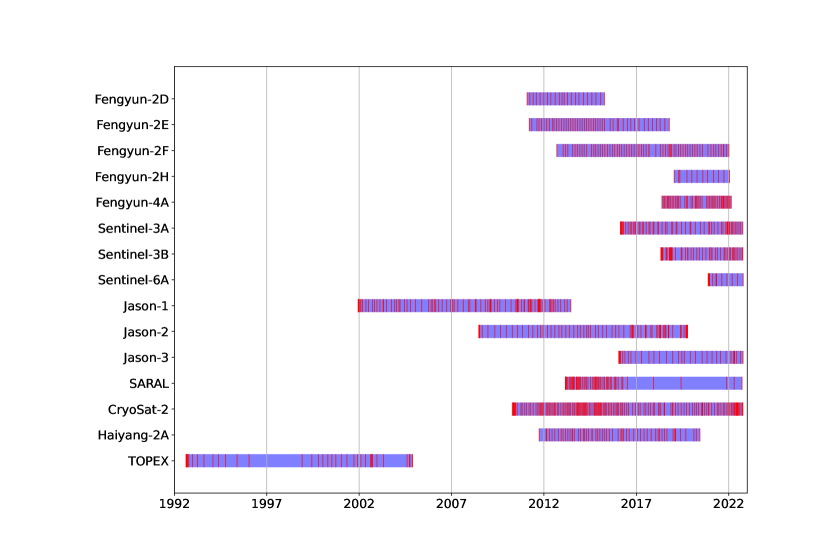
Figure 7: Time periods of satellite observation data sets. Red lines show the timestamps of each manoeuvre. For each satellite, the left point corresponds closely to its launch. The right point either corresponds with its end of life, or when the data was accessed by the authors.

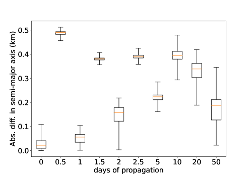
(a) Sentinel-3A

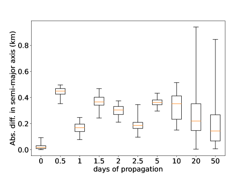
(b) Haiyang-2A

Figure 8: Box plots showing the distribution of propagation errors using SGP4/SDP4. Randomly chosen TLEs are propagated for the number of days shown on the $x$ axis. The propagated values are then compared with accurate data derived from DORIS ground beacons [6]. The large fluctuations in the mean of the propagation errors for small numbers of days of propagation is due to the known periodicity in the propagation errors of SGP4/SDP4 [5]. This periodicity makes it difficult to suggest a cutoff point beyond which the accuracy of the propagator is considered insufficient.

5.1 Manoeuvre Timestamps

The manoeuvre timestamps are stored in YAML files [2]. These files also contain the satellite name and SATCAT catalogue number [17] as metadata. For all satellites other than the Fengyung satellites, these were obtained from the International DORIS Service. Specifically, they were downloaded from ftp.ids-doris.org/pub/ids/satellites/ on the 24th of October 2022. Documentation on file formats can be obtained at that location. Note that, although there is no ground-beacon data available for the TOPEX satellite from the International DORIS Service, its manoeuvres were obtained from this source. Manoeuvre timestamps were extracted from the downloaded files and packaged into the YAML files in this dataset. Orbit control information for Fengyung satellites is provided by China’s National Satellite Meteorological Center on its official website www.nsmc.org.cn/nsmc/en/news/index.html. These manoeuvre events have been collected and shared by colleagues from Purple Mountain Observatory. footnote 4 shows the dates of the first and last manoeuvres for each satellite in the dataset, along with the number of manoeuvres. The period spanned by the manoeuvre data for each satellite is also visualised in Figure 7.

5.2 TLE Data

The TLE data is stored in plain-text files in accordance with the specification provided by NORAD [1]. This data was downloaded from space-track.org (a service provided by NORAD) on 26 October 2022. The files contain all TLE data from 1 week before the first manoeuvre in the associated manoeuvre file until 1 week after the last manoeuvre. footnote 4 shows the number of TLE epochs present in the data for each satellite. This TLE data is easily obtained. We incorporate it as part of this benchmark dataset in order to provide a standardised dataset (particularly with respect to start and end dates) on which to test methodologies for space situational awareness.

5.3 Accurate Satellite Position Data

The benchmark dataset also contains highly accurate (relative to TLE) satellite positions for a subset of satellites. This data is obtained from the DORIS network of ground beacons [6], where it was available. These beacons emit radio signals which are received by the satellites. Satellite positions can then be determined from the Doppler shift of the received signals. The derived satellite positions are highly accurate (on the order of centimeters) and published at 1 minute intervals.

This data was obtained from doris.ign.fr/pub/doris/products/orbits/ on the 28th of September 2022. The availability of this data for each satellite is shown in footnote 4.

The original data is stored in files with the SP3-c format [13]. As this file format requires specific software to manipulate , we have made it available in a more accessible format. Moreover, the positions in this data are recorded in the Geocentric Celestial Reference Frame [29]. They were converted into Keplerian elements [24], before being written to CSV files. These files contain the timestamp of each record, along with the osculating Keplerian elements.

5.4 Evaluation of SGP4/SDP4 Accuracy in this Dataset

As the SGP4/SDP4 propagation model [41] is extensively used for anomaly detection applied to TLE data, it is valuable to establish its accuracy for use in conjuction with this dataset. In particular, we are interested in how its accuracy deteriorates over propagation length. To gain an understanding of the accuracy of this propagator, we investigated the propagation errors on two satellites for which the high-precision DORIS beacon data is available [6]. For each of these satellites, 100 TLE epochs (which fell within the range spanned by the DORIS beacon data) were chosen randomly. At each randomly chosen epoch, the timestamp in the DORIS data that is closest to the given epoch is found. This timestamp is taken to be the starting point of the propagation. As the TLE data is sampled around once per day and the DORIS data is sampled every minute, the chosen timestamp in the DORIS data will align closely with the TLE epoch. SGP4 is then used to convert the mean orbital elements in the TLE data into osculating elements, at the chosen timestamp. These osculating elements are then compared with osculating elements obtained by converting the DORIS positions into osculating Keplerian elements. SGP4/SDP4 is also used to propagate the TLE data to timepoints at set intervals in the future from the originally found DORIS timestamp. Comparisons with the DORIS data are also made at these time points.

Plots of the distributions of these propagation errors are shown in Figure 8. One item that stands out in these plots is that, although the mean propagation error increases with the length of the propagation, this increase is not monotonic. Indeed, the mean error undergoes some sharp drops as we increase the propagation length. This is due to the known periodicity in SGP4/SDP4 errors along propagation length [5, 12, 7]. The conclusion is that some additional care is needed in multiple-time-step propagation, but that it can potentially be very useful, even up to fairly long time steps.

6 Discussion

As described in Section 3, TLE data is intended to be used in conjunction with the full SGP4/SDP4 propagation model [17, 41, 43]. This makes sense for the majority of the cases where one might be using TLE data. For instance, if we want to know where in the night sky to look for a satellite, we need an accurate position for the satellite at the current instant. This position cannot be arrived at from the mean elements in the TLE data used in isolation.

However, if we are interested in the longer-term trends in a satellite’s orbit, such as whether the shape of its orbit on a given day is different from this shape on the previous day, then the SGP4/SDP4 model is not only of far less value, but it has the potential to be the cause of misleading results. We argue that, if one is interested in analysing long-term changes in satellite orbits, then the full SGP4/SDP4 model should be ignored. It is intended for a different task: predicting relatively precise satellite positions at a given instant in time. Rather, one should focus on the mean orbital elements as recorded in the raw TLE values. Propagation of these values, according to some model of orbital mechanics, can be a useful step in an analysis pipeline, however, we suggest that this should be done using some method for propagating only mean orbital elements. Indeed, SGP4/SDP4 first propagates the mean orbital elements (see page 12 of [15]), before adding in non-Keplerian terms. Using just this component of the model would be appropriate.

Section 4.1 examined specific potential negative consequences of utilising SGP4/SDP4 for the long-term analysis of satellite orbits. It focussed on the use of SGP4/SDP4 for propagating TLE values to the epoch time of another satellite in order to compare values. It was shown how using the full SGP4/SDP4 model in this context could magnify the deltas in unpredictable ways (as compared to just propagating the mean elements). Section 4.2 looked at the use of SGP4/SDP4 in order to incorporate non-Keplerian components of the orbit before applying subsequent analysis. It was demonstrated how, if this approach was followed, one would need to ensure that the resulting time series were sampled at a rate much higher than the original TLE data to avoid aliasing. Moreover, a specific case where subtle changes in how NORAD chose epoch times had a drastic impact on the osculating elements at TLE epochs was highlighted. Finally, Section 4.3 looked at the potentially severe scenario where TLEs propagated using the full SGP4/SDP4 model are compared against raw TLE values in subsequent epochs. Not only is this not an apples-to-apples comparison, but it can also cause the introduction of errors due to aliasing effects.

While our analysis has not shown that the addition of non-Keplerian components to TLE data using SGP4/SDP4 will lead to negative consequences in all cases when analysing long-term satellite trends, we do not believe that it is necessary to do so. It is possible that there might be positive effects to incorporating these terms for some satellite. However, we argue that, in any data analysis task, the default approach should be to analyse the raw records. Transformation of these raw records according to some model of dynamics should only be done if this transformation can be demonstrated to provide value. This paper calls into question the value that is provided by transforming TLE data using SGP4/SDP4 when analysing satellite lifetimes. Practitioners should be hesitant to use it for this task until someone can demonstrate its effectiveness.

As summarised in Section 2, there is a large body of existing work on methods for observing changes in satellite orbits over long periods of time from TLE data. However, as different studies choose different satellites on which to evaluate their methods, it is very difficult to compare these approaches. Moreover, it is common for approaches to only be validated on one or two satellites, thus limiting the conclusions that can be made about their effectiveness. To remedy this situation, we have provided an open, curated benchmark dataset which contains the TLE data and associated ground-truth manoeuvre timestamps for a set of 15 satellites. This dataset is described in Section 5.

7 Conclusion

In this paper, we studied the task of analysing trends in satellites’ orbits using TLE data. We demonstrated how using the SGP4/SDP4 orbital propagator for this task, as is regularly done in the literature, can cause significant problems. We have argued that a more fruitful approach would be to propagate the mean orbital elements contained in the TLE records. We have also presented and described an open curated dataset of TLE records and ground-truth manoeuvre timestamps. It is hoped that this new dataset will facilitate future research in this area.

One main avenue for future research is to expand the presented dataset to include more satellites. The authors also hope to investigate the use of mean element propagation for the purpose of detecting anomalies in TLE data.

8 Acknowledgement

We thank Ms Can Zhu and Dr Tinglei Zhu from Key Laboratory for Space Object and Debris Observation, Purple Mountain Observatory, Chinese Academy of Sciences for kindly sharing Fengyun manoeuvring data. We thank Will Heyne of BAE Systems for helpful insights throughout the course of this research. Funding for this work was provided by the SmartSat CRC, project P2.11 .

Appendix A Frequency-space Analysis of High-Resolution Data

The figures in this section show the fourier power spectrum of the osculating semi-major axis (Figure 9), eccentricity (Figure 10) and inclination (Figure 11) for a subset of the satellites in the presented benchmark dataset. These satellites were chosen as they are the ones for which highly accurate orbital data from DORIS ground beacons [6] is available. The analysis presented in these figures was performed on that data. It is worth noting that all three of these orbital elements have dominant frequencies at twice the orbital frequency. The orbital period of low-earth orbit satellites (which includes many satellites in the benchmark dataset) is in the region of 2 hours [35]. This implies that if we sample these osculating components at the frequency of TLE epoch updates (around once per day), we should expect these components to be aliased. This is the root cause behind the pitfalls discussed in Section 4.2 and Section 4.3.

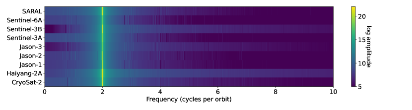
Figure 9: Fourier power spectrum of the semi-major axis of a sample of satellites from the presented dataset. The data used for this figure is derived from DORIS ground beacons [6]

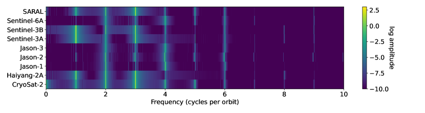
Figure 10: Fourier power spectrum of the eccentricity of a sample of satellites from the presented dataset. The data used for this figure is derived from DORIS ground beacons [6]

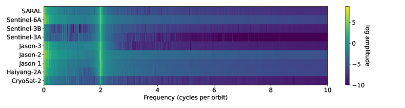
Figure 11: Fourier power spectrum of the inclination of a sample of satellites from the presented dataset. The data used for this figure is derived from DORIS ground beacons [6]

Appendix B Additional Plots Concerning Pitfall One

This appendix contains extra plots demonstrating the first pitfall, as discussed in Section 4.1. They were excluded from that section for the purpose of brevity. Whereas Figure 3 shows plots of propagation residuals in the radial direction and along the semi-major axis, Figure 12 includes residuals in the in-track and cross-track directions. Similarly, Figure 13 and Figure 14 include residuals in the eccentricity and inclination.

(a) Radial position difference

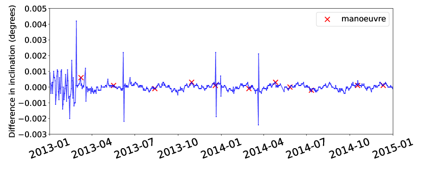
(b) In-track position difference

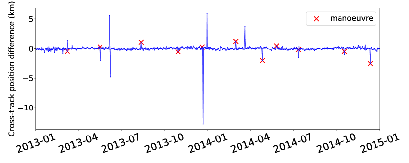
(c) Cross-track position difference

Figure 12: The difference between propagated TLE positions and positions taken from the TLE in the subsequent epoch. The TLE from each epoch is propagated to the subsequent epoch using the SGP4/SDP4 model. SGP4/SDP4 is also used to incorporate non-Keplerian terms into the TLE recorded at the subsequent epoch and arrive at precise positions. This analysis is plotted for the Jason 2 satellite. The red crosses show the manoeuvre times, obtained independently from the TLE data. These plots should be contrasted with those in Figure 13, which show the differences in Keplerian elements. Observe how, for none of the three directions plotted, do the large propagation errors align particularly well with the manoeuvre timestamps.

(a) Difference in osculating semi-major axes

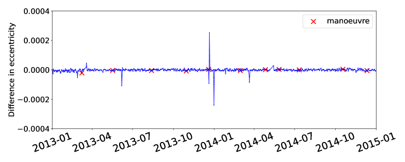
(b) Difference in osculating eccentricities

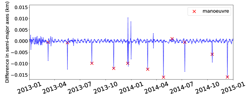
(c) Difference in mean semi-major axes

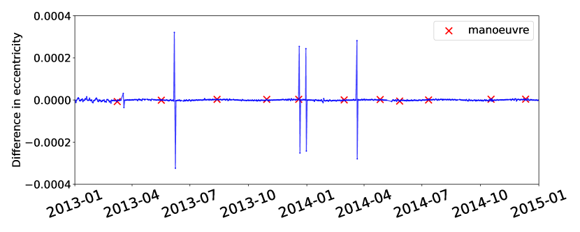
(d) Difference in mean eccentricities

(e) Difference in osculating inclinations

(f) Difference in mean inclinations

Figure 13: Compares different propagations of TLE data to the observed orbital elements at the subsequent epoch. (13(a)), (13(b)) and (13(e)) plot the results of using the full SGP4 algorithm (including non-Keplerian terms) to propagate the TLE from each epoch to the subsequent epoch. The SGP4 algorithm is also used to add the high frequency terms at the subsequent epoch in order to arrive at osculating Keplerian elements. The difference between the propagated and non-propagated elements is then found. (13(c)), (13(d)) and (13(f)), by contrast, show the results of propagating TLEs using only the low-frequency terms of SGP4, resulting in propagated mean elements. These elements are then compared directly against the TLE elements in the subsequent epoch. The plots show this analysis for the Jason 2 satellite. The red crosses show the manoeuvre times, obtained independently from the TLE data. A number of differences between these approaches can be observed. The propagation errors for the inclination contain substantially less noise when this is done using the mean elements. On the other hand, the computation of these errors for the eccentricity appears quite unstable.

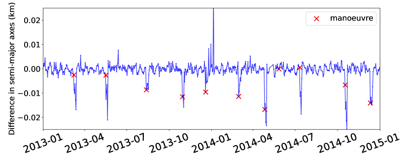
(a) Difference in osculating semi-major axes

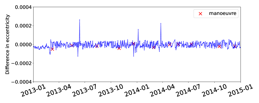
(b) Difference in osculating eccentricities

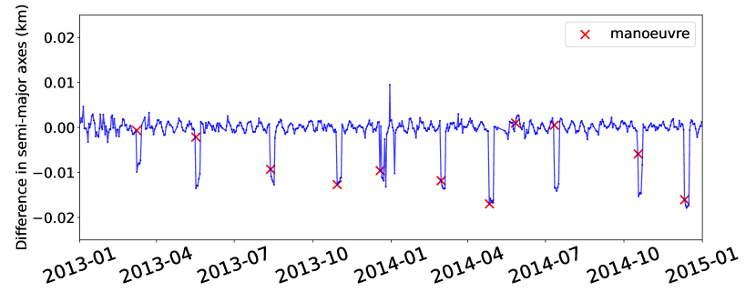
(c) Difference in mean semi-major axes

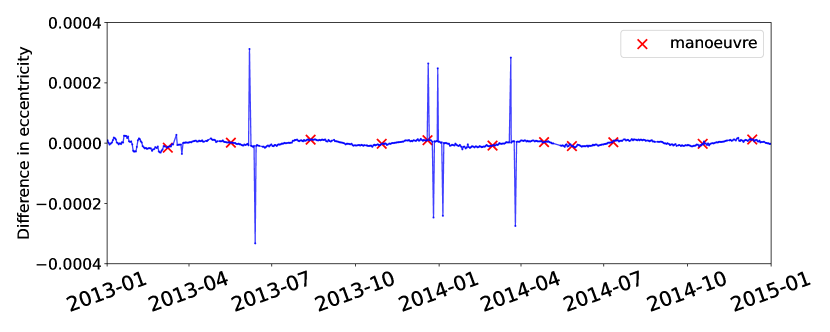
(d) Difference in mean eccentricities

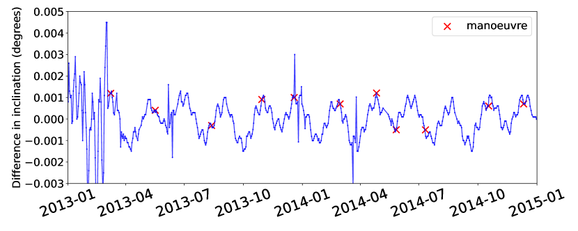
(e) Difference in osculating inclinations

(f) Difference in mean inclinations

Figure 14: Compares different propagations of TLE data to the observed orbital elements five epochs later. Contains the same plots as Figure 13, but the propagation is performed over 5 epochs as opposed to 1. We observe significantly more noise when the propagations are performed using the full SGP4/SDP4 model (that is, by comparing osculating elements), as compared to only propagating the mean elements.

References

- [1] CelesTrak: NORAD two-line element set format. celestrak.org/NORAD/documentation/tle-fmt.php. Accessed: 2022-10-24.
- [2] YAML ain’t markup language (YAMLTM) version 1.2. yaml.org/spec/1.2.2/. Accessed: 2022-10-24.
- [3] 18th Space Control Squadron. Spaceflight safety handbook for satellite operators. In Tech. Rep. 1.5, Combined Force Space Component Command Vandenberg Air Force Base, California, USA, 2020.
- [4] A Águeda, L Aivar, J Tirado, and JC Dolado. In-orbit lifetime prediction for LEO and HEO based on orbit determination from TLE data. In 6th European Conference on Space Debris, volume 723, page 61, 2013.
- [5] Saika Aida and Michael Kirschner. Accuracy assessment of SGP4 orbit information conversion into osculating elements. In 6th European Conference on Space Debris, 2013.
- [6] A Auriol and C Tourain. DORIS system: the new age. Advances in space research, 46(12):1484–1496, 2010.
- [7] Xian-Zong Bai, Lei Chen, and Guo-Jin Tang. Periodicity characterization of orbital prediction error and Poisson series fitting. Advances in space research, 50(5):560–575, 2012.
- [8] Xue Bai, Chuan Liao, Xiao Pan, and Ming Xu. Mining two-line element data to detect orbital maneuver for satellite. IEEE Access, 7:129537–129550, 2019.
- [9] Roger R Bate, Donald D Mueller, Jerry E White, and William W Saylor. Fundamentals of astrodynamics. Courier Dover Publications, 2020.
- [10] Christopher L Bowman and Paul Zetocha. Abnormal orbital event detection, characterization, and prediction. In AIAA Infotech @ Aerospace, page 0365. 2015.
- [11] Jacob Decoto and Patrick Loerch. Technique for GEO RSO station keeping characterization and maneuver detection. In Advanced Maui Optical and Space Surveillance Technologies Conference, page 42, 2015.
- [12] PF Easthope. Examination of SGP4 along-track errors for initially circular orbits. IMA Journal of Applied Mathematics, 80(2):554–568, 2015.
- [13] Steve Hilla. The extended standard product 3 orbit format (SP3-c). Technical report, National Geodetic Survey, National Ocean Service, 2010.
- [14] David Hoese. pyorbital. github.com/pytroll/pyorbital. Accessed: 2022-11-02.
- [15] Felix R Hoots and Ronald L. Roehrich. Models for propagation of NORAD element set. Technical Report 3, Aerospace Defense Command, United States Air Force, 1980. Spacetrack report No.3.
- [16] Tom Kelecy, Doyle Hall, Kris Hamada, and Dennis Stocker. Satellite maneuver detection using two-line element (TLE) data. In Proceedings of the Advanced Maui Optical and Space Surveillance Technologies Conference. Maui Economic Development Board (MEDB) Maui, HA, 2007.
- [17] T.S. Kelso. Frequently asked questions: Two-line element set format. celestrak.org/columns/v04n03/. Accessed: 2022-10-26.
- [18] Bill Kraus, Duane DeSieno, Derek M Surka, Gary Haith, and Christopher Bowman. Detecting abnormal space catalog updates. In Infotech@ Aerospace, 2012.
- [19] Stijn Lemmens and Holger Krag. Two-line-elements-based maneuver detection methods for satellites in low earth orbit. Journal of Guidance, Control, and Dynamics, 37(3):860–868, 2014.
- [20] Stijn Lemmens and Holger Krag. Two-line-elements-based maneuver detection methods for satellites in low earth orbit. Journal of Guidance, Control, and Dynamics, 37(3):860–868, 2014.
- [21] Tao Li, Kebo Li, and Lei Chen. New manoeuvre detection method based on historical orbital data for low earth orbit satellites. Advances in Space Research, 62(3):554–567, 2018.
- [22] Tao Li, Kebo Li, and Lei Chen. Maneuver detection method based on probability distribution fitting of the prediction error. Journal of Spacecraft and Rockets, 56(4):1114–1120, 2019.
- [23] Robert J Marks II. Handbook of Fourier analysis & its applications. Oxford University Press, 2009.
- [24] Jean Meeus. Astronomical Algorithms. Willman-Bell, 1991.
- [25] Andrea Milani, Anna Maria Nobili, and Paolo Farinella. Non-Gravitational Perturbations and Satellite Geodesy. 1987.
- [26] Arvind Mukundan and Hsiang-Chen Wang. Simplified approach to detect satellite maneuvers using TLE data and simplified perturbation model utilizing orbital element variation. Applied Sciences, 11(21):10181, 2021.
- [27] A Pastor, G Escribano, A Cano, M Sanjurjo-Rivo, C Pérez, I Urdampilleta, and D Escobar. Manoeuvre detection and estimation based on sensor and orbital data. In Proc. 8th European Conference on Space Debris (virtual), Darmstadt, Germany, 20–23 April 2021, pages 1–13. ESA Space Debris Office, 2021.
- [28] Russell P Patera. Space event detection method. Journal of Spacecraft and Rockets, 45(3):554–559, 2008.
- [29] Gérard Petit and Brian Luzum. IERS conventions (2010) - IERS technical note no. 36. Technical report, International Earth Rotation and Reference System Service, 2010.
- [30] Laura Pirovano and Roberto Armellin. Detection and estimation of spacecraft maneuvers for catalog maintenance. arXiv preprint arXiv:2210.14350, 2022.
- [31] Brandon Rhodes. python-sgp4. github.com/brandon-rhodes/python-sgp4. Accessed: 2022-11-02.
- [32] Brandon Rhodes. python-skyfield. github.com/brandon-rhodes/python-skyfield. Accessed: 2022-11-02.
- [33] Thomas G Roberts and Richard Linares. Geosynchronous satellite maneuver classification via supervised machine learning. Technical report, Massachusetts Institute of Technology, 2021.
- [34] Hanspeter Schaub and John L Junkins. Analytical mechanics of space systems. AIAA, 2003.
- [35] George Sebestyen, Steve Fujikawa, Nicholas Galassi, and Alex Chuchra. Low Earth Orbit Satellite Design. Springer, 2018.
- [36] Charlotte Shabarekh, J Kent-Bryant, M Garbus, G Keselman, J Baldwin, and B Engberg. Efficient object maneuver characterization for space situational awareness. In 32nd Space Symposium, Technical Track, Colorado Springs, Colorado, United States of America. Presented on April, pages 11–12, 2016.
- [37] Charlotte Shabarekh, Jordan Kent-Bryant, Gene Keselman, and Andonis Mitidis. A novel method for satellite maneuver prediction. In Advanced Maui Optical and Space Surveillance Technologies Conference, page 11, 2016.
- [38] S Shivshankar and Debasish Ghose. Behaviour modelling of satellites for space situational awareness using time series analysis and k-means clustering. In 2021 IEEE International Conference on Electronics, Computing and Communication Technologies (CONECCT), pages 1–6. IEEE, 2021.
- [39] WD Song, RL Wang, and J Wang. A simple and valid analysis method for orbit anomaly detection. Advances in Space Research, 49(2):386–391, 2012.
- [40] Raymond Swartz, John Coggi, and Justin McNeill. A swift sift for satellite event detection. In AIAA/AAS Astrodynamics Specialist Conference, page 7527, 2010.
- [41] David Vallado, Paul Crawford, Ricahrd Hujsak, and TS Kelso. Revisiting spacetrack report #3. In AIAA/AAS Astrodynamics Specialist Conference and Exhibit, page 6753, 2006.
- [42] David A Vallado. Fundamentals of astrodynamics and applications, volume 12. Springer Science & Business Media, 2001.
- [43] David A Vallado and Paul J Cefola. Two-line element sets - practice and use. In 63rd International Astronautical Congress, Naples, Italy, pages 1–14, 2012.
- [44] Dongfang Wang and Fen Li. A machine learning method for the orbit state classification of large LEO constellation satellites. Advances in Space Research, 2022.
- [45] Yiran Wang, Xiaoli Bai, Hao Peng, Genshe Chen, Dan Shen, Erik Blasch, and Carolyn B Sheaff. Gaussian-binary classification for resident space object maneuver detection. Acta Astronautica, 187:438–446, 2021.
- [46] Shengxian Yu, Xin Wang, and Tinglei Zhu. Maneuver detection methods for space objects based on dynamical model. Advances in Space Research, 68(1):71–84, 2021.
- [47] Yang Zhao, Kefei Zhang, James Bennett, Jizhang Sang, and Suqin Wu. A method for improving two-line element outlier detection based on a consistency check. In Proceedings of the Advanced Maui Optical and Space Surveilllance (AMOS) Technologies Conference, Maui, Hawaii, 2014.