MTMD: Multi-Scale Temporal Memory Learning and Efficient Debiasing Framework for Stock Trend Forecasting

Abstract

Recently, machine learning methods have shown the prospects of stock trend forecasting. However, the volatile and dynamic nature of the stock market makes it difficult to directly apply machine learning techniques. Previous methods usually use the temporal information of historical stock price patterns to predict future stock trends, but the multi-scale temporal dependence of financial data and stable trading opportunities are still difficult to capture. The main problem can be ascribed to the challenge of recognizing the patterns of real profit signals from noisy information. In this paper, we propose a framework called Multiscale Temporal Memory Learning and Efficient Debiasing (MTMD). Specifically, through self-similarity, we design a learnable embedding with external attention as memory block, in order to reduce the noise issues and enhance the temporal consistency of the model. This framework not only aggregates comprehensive local information in each timestamp, but also concentrates the global important historical patterns in the whole time stream. Meanwhile, we also design the graph network based on global and local information to adaptively fuse the heterogeneous multi-scale information. Extensive ablation studies and experiments demonstrate that MTMD outperforms the state-of-the-art approaches by a significant margin on the benchmark datasets. The source code of our proposed method is available at https://github.com/MingjieWang0606/MDMT-Public.

1 Introduction

With the development of information technology and financial technology, stock speculation has emerged as one of the most popular and eagerly awaited forms of investment. Stock trend forecasting has become an important way for people to study the stock market by analyzing and forecasting the trend of the stock market by various artificial and technical means [1]. However, the unpredictability of stock information and the ubiquitous noise persist, such as the random dynamic and non-stationary behaviors of markets and customers, the asymmetric information and the “noisy” behaviors of traders, all of which hinder the accurate prediction of trends [2]. Therefore, it is necessary to take the shadow knowledge of the above-mentioned implicit or explicit biases into account to provide more accurate prediction.

Recently, machine learning applications used for stock trend forecasting have shown their potential to bring significant returns [3, 4, 5]. In order to optimize the forecasting performance, it is common practice to analyze the market movement by inputting relevant features into the model, so as to mine fundamental and technical factors in the temporal information of historical price patterns. Generally, models such as Transformers [6], Long Short Term Memory (LSTM) [7], and Gated Recurrent Unit (GRU) [8, 9], exploit a variety of features based on price, relationship, and sequential information to capture non-linear patterns in multivariate time series. In order to make further use of the potential interdependence of different factors, a series of approaches have been proposed. For example, State Frequency Memory (SFM) [10] uses the discrete Fourier transform to capture multi-frequency trading patterns. In addition, hierarchical concept-oriented shared information mining (HIST) for stock trend forecasting [11] and Graph ATtention networks (GATs) [12] regard variables as nodes to construct graphs, so as to mine the interactions among concerned variables within the same timestamp.

However, there are two main issues in the above-mentioned work that have not been fully considered. On the one hand, the inconsistency of data distribution between the training data and the real-world data is difficult to deal with by using empirical knowledge-based modeling, which can lead to over-fitting and extreme inductive bias. Specifically, a basic principle of empirical design is that the underlying rules can be applied to a variety of situations. However, modeling is usually done through a set of processes based on expert knowledge, which makes it difficult for them to adapt to the ever-changing noise distribution in the stock movement, which greatly limits the actual profitability of the model. On the other hand, market frictions have short-term constraints on the market, resulting in a price pressure effect. The final stable point and instantaneous return of each price pressure effect provide an estimate of long-term and short-term effects of this constraint, and together with noise from the original stock data, it constitutes the price noise to varying degrees. The above problems exist simultaneously, interacting with each other in a fluctuating market, which will further increase the risk of model forecasting. Therefore, we believe that current model overemphasizes mixed noise patterns while completely missing and misinterpreting real profit signal patterns.

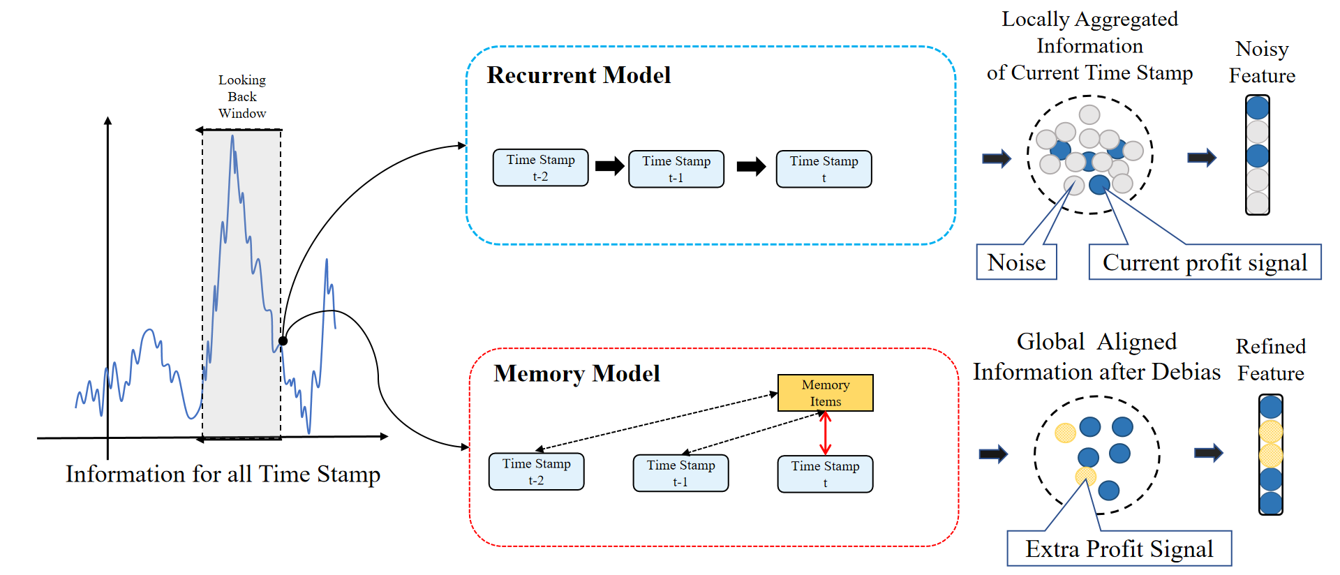
Figure 1: Illustration of recurrent model and memory model in the real stock market. The recurrent model only depends on the state at $t-1$, and it will tend to learn the noise patterns from historical data. However, the memory will span the global information flow with multiple previous timestamps, which helps the model capture extra profit signals for the current timestamp. In addition, the local aggregation will fit the noise in the current data. The memory model uses global alignment and uses the knowledge collected in the past to achieve denoising.

In order to address these problems, it is important to effectively capture profit signals in the noisy data and clearly summarize their general characteristics. Unfortunately, like the problems encountered by most existing methods [7, 8], this kind of signals is too rare and vague to be found in every timestamp of local batch processing. In the previous literature, it is suggested that Recurrent Neural Network (RNN) based methods have a poor performance in stock trend forecasting. Shown as the recurrent model in Figure 1, considering at timestamp $t$, its state only depends on the state at timestamp $t-1$. On the contrary, if we consider the global information flow, the profit signals may be connected as a meaningful trace that spans different timestamps. Therefore, our motivation is to retain the most important information and pass it on in different training steps to track the pattern of profit signals. In our method, shown as the memory model in Figure 1, the memory records general representative patterns of previous states and then works as a retrieve base in processing the state at timestamp $t$ to achieve temporal consistency. Here, the temporal consistency implies that the previous states from timestamp $0$ to $t-1$ participate in determining the state at timestamp $t$ together. Moreover, compared to Transformer, the quadratic complexity of Transformer leads to slow training for long sequences. However, the memory model saves all the important information from $0$ to $t-1$, and it does not need to traverse the whole batch data. In this way, when training the model, the complexity would be significantly reduced from $\mathcal{O}(t^{2})$ to $\mathcal{O}(t)$.

In this paper, we propose a Multi-scale Temporal Memory learning and efficient Debiasing (MTMD) framework for stock trend forecasting. Particularly, to achieve temporal consistency, we introduce a memory model based on HIST [11], which can mine the concept-oriented shared information from predefined concepts and hidden concepts. It can transfer summarized long-range profit features of all previous timestamps to current timestamp that can be seen in Figure 1. Specifically, in order to avoid excessive complexity, a learnable embedding of each stock with external attention is adopted, in which each individual element in this embedding corresponds to a representative profit signal at the stock level. This manner would be free from time intervals and group stocks via their self-similarity. Moreover, to ensure temporal consistency, the memory block will suppress all irrelevant noises and stocks according to all past feature of similarity. After that, aiming to verify the proposed MTMD, a large number of experiments are carried out on real-world stock market datasets. They are compared with nine baselines. Our result shows that MTMD outperforms other baselines in various evaluation metrics. Specifically, the approach outperforms the strongest baseline with an improvement of up to 6.0% and 4.3% in information coefficient (IC) [13] and Rank IC [14] scores, where IC is the pearson correlation coefficient and Rank IC is spearman’s rank correlation coefficient between the real and predicted change rates. In addition to further verifying the reliability of our MTMD, more analysis has been done to examine the impact of each individual component. The contribution is shown as follows.

1. We develop a new framework, MTMD, to capture and record the patterns of actual profit signals hidden in the information flow by using a memory block, thus reducing the impacts of the temporal inconsistency in empirical design and extreme model deviation.

2. We propose a strategy to process features at different levels. It allows for comprehensive mining of local information and disaggregation at global and local scales to understand more representative stock features in response to stock shocks at different levels.

3. We conduct extensive experiments on real stock market data. The results show that we achieve a new state-of-the-art (SOTA) performance on standard benchmarks and improves 6% and 4% compared to the previous SOTA in IC and Rank IC. Meanwhile, The validity of our MTMD framework is also validated.

Organization: The remainder of this paper can be organized as follows. Section 2 introduces background concepts and related work on stock trend forecasting. Section 3 and 4 describes our proposed approach. Section 5 presents experiments and discusses our findings. Finally, Section 6 concludes our paper and provides some feasible directions for the future work.

2 Related Works

In this section, we review the research on stock trend forecasting from the early machine learning models to the latest deep learning models. Besides, we summarize the shortcomings of existing models, even discuss the characteristics of the financial data and the practical application of the models. Finally, we explain how our method can fill in the gaps in the existing models.

Machine Learning Research in Financial Markets. The general data of stocks are mainly composed of price and trading volume in different time periods. Due to the huge market with lots of interfering factors, data of stocks presents the characteristics of non-stable, nonlinear and high noise. In machine learning, early Autoregressive Model (AR) [15] and Autoregressive Integrated Moving Average Model (ARIMA) [16] relied heavily on linear relationships so they did not perform well in the field of stock prediction. The structure of the tree models [17, 18, 19, 20, 21] can find the complex nonlinear relationship between the features by calculating the importance, but the stock data is often unbalanced, thus the calculation result of the decision tree is locally optimal rather than globally optimal, which is easy to lead to the problem of overfitting. Genetic Algorithm (GA) [22, 23, 24] can achieve global optimization through continuous iteration. However, stocks in the market not only have systemic risks, but also high similarity in a period of time accompanied by industry rotation and extreme events, thus GA is prone to premature convergence and cannot jump out of local search. Hidden Markov Model (HMM) [25] only depends on the probability of a state before current time. Although it can avoid historical invalid information and market noise, it has great weakness in mining and learning the features of long time series because of its non-memory. Therefore, if we want to use more known information, we must establish high-order Markov Random Fields (MRFs) or memory block. Therefore, the main shortcoming of the traditional machine learning models is that it cannot coordinate the optimal local and global features to adapt to the multi-frequency changes of nonlinear stock data. Our method uses multi-scale aggregation to search for local features and collect global features that uses a memory block to capture effective features at the same time, which greatly enhances the universality and stability of the model in different time series. In addition, the traditional machine learning model is still highly dependent on expert knowledge and has poor self-learning ability, thus it is easy to fall behind with the changes of the market. We hope to introduce the framework of deep learning to make the model better adapt to the current market.

Deep Learning Research in Financial Markets: Because the stock data has the characteristics of high noise and low signal-to-noise ratio, the model needs to be able to adapt to market disturbances better. The deep learning framework has strong learning ability, and it is superior to traditional machine learning in nonlinear and complex tasks by using efficient feature expression. On the one hand, Recurrent Neural Network (RNN) is the first successful deep learning model to address time series data, but it is hard to overcome the gradient explosion and gradient disappearance during training. Then, LSTM [7, 26, 27] and GRU [8, 28] networks can grasp the influence of historical information on the current state by setting the gate unit, and overcome the drawbacks of RNN. However, this model heavily relies on step-by-step prediction and unable to learn long sequences effectively. Zhang et al. [10] create a SFM, which requires the memory state to be decomposed into frequency components by Fourier transform, thus providing fine-grained multi-frequency analysis to establish the dependency model in the frequency domain. Nevertheless, the SFM is sensitive to high dimensional data and extreme events. ALSTM [29] and Transformer [6] frameworks combine the attention mechanism with a dual-stage RNN, proving that attention mechanism is effective for mining global temporal information. However, there are still a few problems in neural network models based on RNN framework because of the inability to capture long distance information and the large amount of computation. On the other hand, Graph Neural Network (GNN) is proposed to establish the correlation among stock concepts [30]. Kim et al. [31] present a hierarchical attention network for stock prediction (HATS) based on relational data. GATs [12] leverage masked self-attention layers on graph-structured data in stacked layers. In another study, HIST [11] adopts the idea of mining shared information from graphs constructed from stocks and related concepts. The aggregation of stock-concept features significantly improves the accuracy of prediction. These methods are based on the definition of relationship between stocks by human experts, and pay more attention to the relationship of stocks, while ignoring the pattern influence of sector rotation on noise.

In summary, the key point of deep learning is to learn a truly effective profit signal in a noisy environment. In our method, the MTMD hopes to pay more attention to the low-noise signals in multiple timestamps, which mining cross-stock relationships based on memory blocks.

3 Problem Formulation

The raw stock features of $N_{s}$ target stocks on date $t$ can be denoted by $X^{t}=\{\boldsymbol{x}_{1}^{t},\boldsymbol{x}_{2}^{t},\cdots,\boldsymbol{x}_{N_{s}}^{t}\}$ with $N_{c}$ predefined concepts $C^{t}=\{\boldsymbol{c}_{1}^{t},\boldsymbol{c}_{2}^{t},\cdots,\boldsymbol{c}_{N_{c}}^{t}\}$. Each raw stock feature $\boldsymbol{x}_{i}^{t}$ of stock $i$ on date $t$ is a vector, which contains a collection of features to stock $i$ on date $t$, including opening price, closing price, volume, etc. Here, we need to predict the the stock trend $\hat{\boldsymbol{p}}^{t}=\{\hat{p}_{1}^{t},\hat{p}_{2}^{t},\cdots,\hat{p}_{N_{s}}^{t}\}$ of the input stocks. Therefore, considering a stock $i$ on date $t$, our problem can be formulated as a mapping $f$ (a deep model in our approach) with parameters $\boldsymbol{W}$ such that

$$\hat{p}_{i}^{t}=f(\boldsymbol{x}_{i}^{t},C^{t};\boldsymbol{W}),$$ (1)

where $\hat{p}_{i}^{t}$ is the predicted trend (change rate) and its corresponding ground truth is defined as $p_{i}^{t}=\frac{price^{t+1}-price^{t}}{price^{t}}$, which is the real change rate of stock $i$ from date $t$ to $t+1$. Here, we hope that the predicted trend $\hat{p}_{i}^{t}$ is as close to the real trend $p_{i}^{t}$ as possible.

4 Methodology

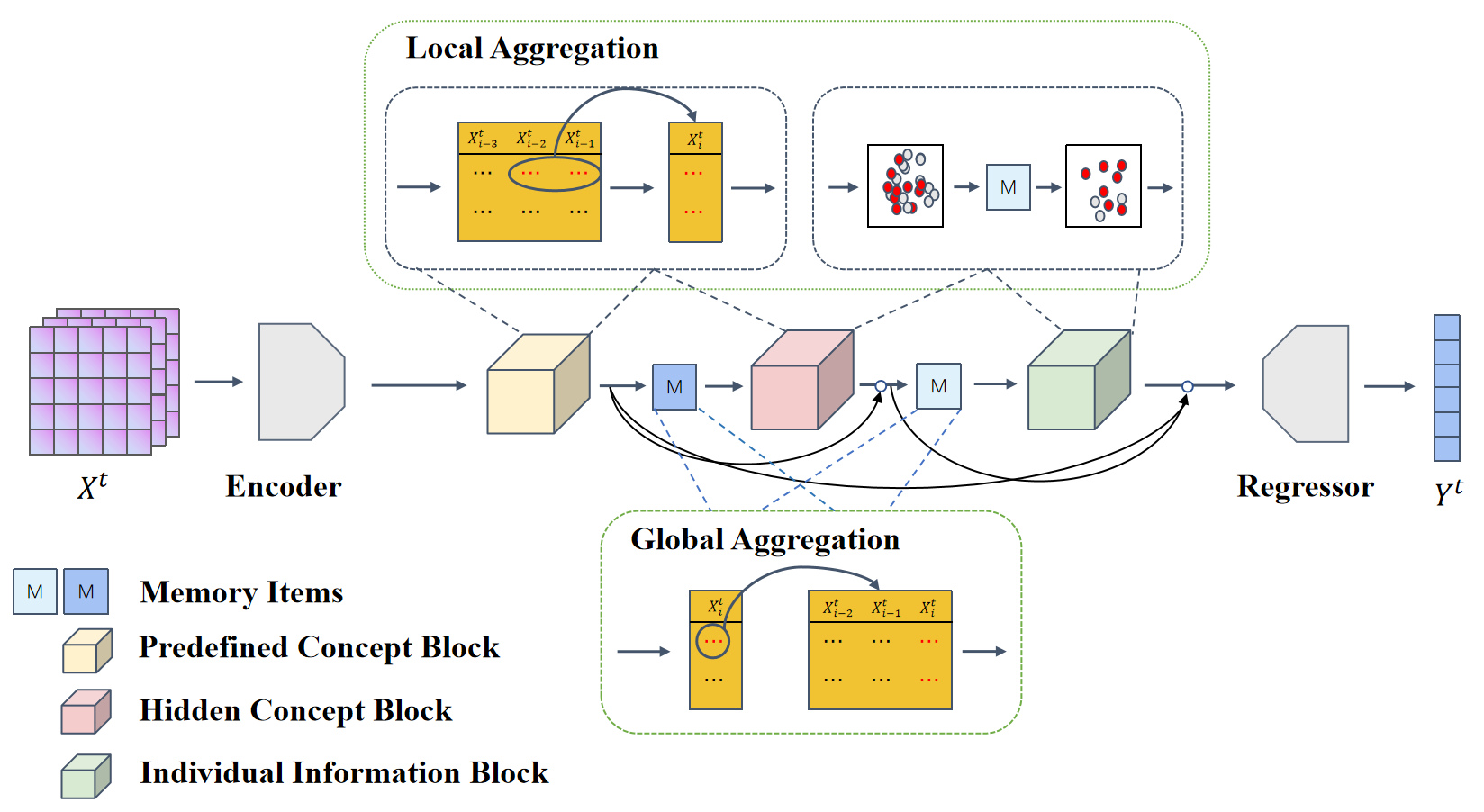
Figure 2: The architecture of our MTMD framework. The global aggregations modules includes predefined concept module, hidden concept module and personal information module. The local aggregation modules includes memory items. And the global and local aggregations modules captures and learn multi-scale time information segments, and is subjected to deviation removal.

4.1 The overview of our MTMD framework

In our approach, we first define a stock-concept feature extractor as the starting point because this is the fundamental component of our MTMD framework. Then, by introducing memory items into the stock-concept feature extractor, we formulate a memory-assisted stock-concept feature extractor to extract deep features from the raw stock feature $X^{t}$. Finally, we can get the prediction $\hat{\boldsymbol{p}}^{t}$ by combining the memory-assisted stock-concept feature extractor and stock trend regressor. The stock trend regressor is a predictor based on the output features from memory-assisted stock-concept feature extractor. Thus, our MTMD framework consists of the memory-assisted stock-concept feature extractor and stock trend regressor. Whether it is the stock-concept feature extractor or the memory-assisted stock-concept feature extractor, they all have three modules: Predefined concept module, hidden concept module, and individual information module. The basic architecture is shown in Figure 2.

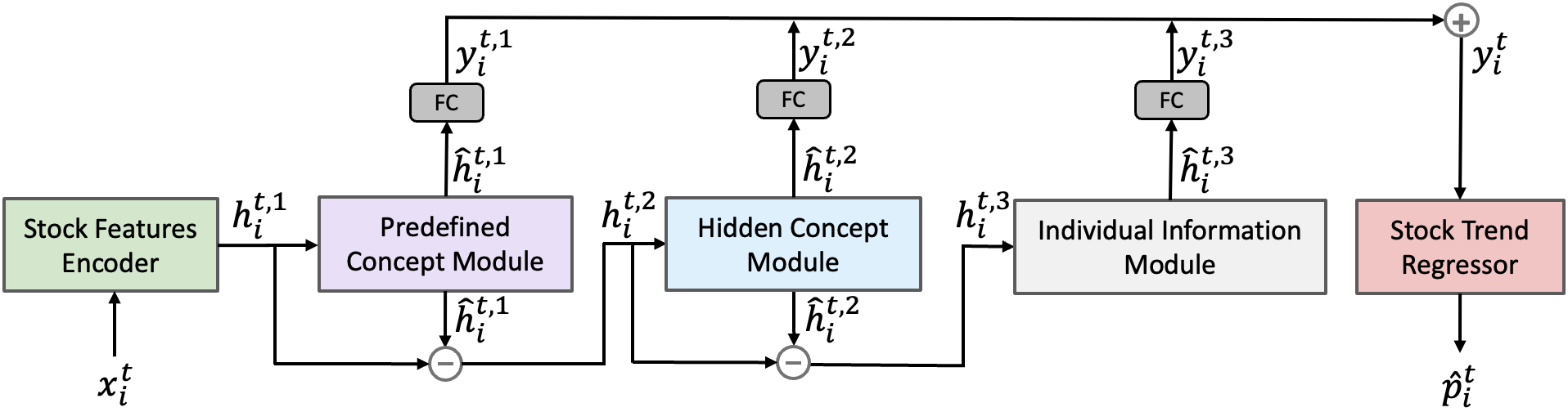
Figure 3: The framework of stock-concept feature extractor.

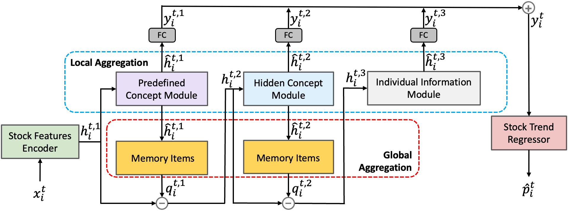
Figure 4: The framework of memory-assisted stock-concept feature extractor.

• Stock-concept feature extractor: It consists of a stock feature encoder and three modules shown in Figure 3: predefined concept module, hidden concept module, and individual information module, which are denoted by $\theta=1,2,3$ respectively. When considering the date $t$ and stock $\boldsymbol{x}_{i}^{t}$, the encoded stock features provide initial temporal embedding $\boldsymbol{h}^{t,1}_{i}\in\mathbb{R}^{L}$ with $\theta=1$ by using historical price data, and then the other three modules further extract various supplementary information using related stock concepts. The modules are organized through doubly residual architecture. For each module $\theta$, we input $\boldsymbol{h}^{t,\theta}_{i}$ obtained from the previous module $\theta-1$ and output the stock-concept feature $\hat{\boldsymbol{h}}^{t,\theta}_{i}\in\mathbb{R}^{L}$. This stock-concept feature $\hat{\boldsymbol{h}}^{t,\theta}_{i}$ contains the effect of its corresponding module, which will be removed from current input feature to generate the input of the next modele. Thus, we have $\boldsymbol{h}^{t,\theta+1}_{i}=\boldsymbol{h}^{t,\theta}_{i}-\hat{\boldsymbol{h}}^{t,\theta}_{i}$. Besides, it can formulate a forecast feature $\boldsymbol{y}^{t,\theta}_{i}\in\mathbb{R}^{L}$ by using a fully connected (FC) network. Finally, we get the eventually extracted feature $\boldsymbol{y}^{t}_{i}=\boldsymbol{y}^{t,1}_{i}+\boldsymbol{y}^{t,2}_{i}+\boldsymbol{y}^{t,3}_{i}$.

• Memory-assisted Stock-concept feature extractor: This framework is shown in Figure 4. We add a memory block for predefined concept module and hidden concept module, where the memory block is composed of $K$ memory items. These memory blocks are global, which collect all information in previous timestamps. The predefined concept module, hidden concept module, and individual information module are trained only in the current timestamp, thus they are local. Here, we can say that memory blocks are global aggregation and other modules are local aggregation. Shown as the blue dotted box in Figure 4, it is the local aggregation, which uses stock-concept feature extractor for local encoding. Shown as red dotted box in Figure 4, it is the global aggregation. For the first two module $\theta\in\{1,2\}$, predefined concept module or hidden concepts module, we input the stock-concept feature $\boldsymbol{\hat{h}}^{t,\theta}_{i}$ to its memory block, and get a low-noise and global feature $\boldsymbol{q}^{t,\theta}_{i}$. This global feature $\boldsymbol{q}^{t,\theta}_{i}$ will be removed from current input feature to generate the input of the next module. Thus, we have $\boldsymbol{h}^{t,\theta+1}_{i}=\boldsymbol{h}^{t,\theta}_{i}-\boldsymbol{q}^{t,\theta}_{i}$.

The stock trend regressor is a feed-forward network, and finally the different types of feature given by the above feature extractor are summarized together to make predictions, which shown in the red block of Figure 4.

4.2 Memory-assisted Stock-concept Feature Extractor

4.2.1 Stock Feature Encoder

The raw stock features of $N_{s}$ target stocks, each stock $i$ on date $t$ is denoted by $\boldsymbol{x}_{i}^{t}\in\mathbb{R}^{L^{\prime}}$, whose elements composed of historical trading prices and volumes of stock $i$ within a looking back window. The stock feature encoder extracts temporal information in them and compress the information as a denser embedding matrix in a lower dimension. As GRU [8] demonstrates the capability of learning sequential information and ability to alleviate gradient vanishing, we apply a 2-layer GRU as our encoder to generate the initial embedding:

$$\boldsymbol{h}^{t,1}_{i}={\rm GRU}(\boldsymbol{x}^{t}_{i}),$$ (2)

where $\boldsymbol{h}^{t,1}_{i}\in\mathbb{R}^{L},L<L^{\prime}$ represents temporal information in stock $i$, and each of them is the row of matrix $\boldsymbol{H}^{t,1}\in\mathbb{R}^{N_{s}\times L}$.

4.2.2 Predefined Concept Block

The predefined concepts are manually defined by a category of stocks, such as different stock market sectors. For example, Google and Facebook are classified as communication services, while Walmart and Coca-Cola are classified as daily consumer goods. These concepts connect companies, and build a bipartite graph of stock concepts, from which meaningful shared information can be mined to obtain more accurate forecasts.

Therefore, the predefined concept module are designed to learn such a dynamic concept embedding from the graph built on each date. Given $N_{c}$ predefined concepts $C^{t}$ on date $t$ and temporal embedding $\boldsymbol{h}^{t,1}$, we initialize the embedding of each concept $\boldsymbol{c}^{t}_{j}$, denoted by $\boldsymbol{e}^{t,1}_{j}$, as the weighted average over the encoded features of stocks connected with the concept:

$$\boldsymbol{e}^{t,1}_{j}=\sum\nolimits_{i\in D^{t,1}_{j}}\alpha^{t}_{i,j}\boldsymbol{h}^{t,1}_{i},$$ (3)

where $\boldsymbol{e}^{t,1}_{j}\in\mathbb{R}^{L}$ is the initial embedding of concept $\boldsymbol{c}^{t}_{j}$ on date $t$, $D^{t,1}_{j}$ is the set of stocks connected with concept $\boldsymbol{c}^{t}_{j}$, and $\alpha^{t}_{i,j}$ is the weight indicating the degree of contribution made by stock $i$ to concept $\boldsymbol{c}^{t}_{j}$. To measure this, we take advantage of the market capitalization $\delta^{t}_{i}$ of stock $i$ on date $t$ and compute its proportion over all connected stocks as

$$\alpha^{t}_{i,j}=\frac{\delta^{t}_{i}}{\sum_{i^{\prime}\in D^{t,1}_{j}}\delta^{t}_{i^{\prime}}}.$$ (4)

The above initial embedding can be learnt from a partially connected graph. However, some of the significant links between stocks and predefined concepts may not be covered by the input data, while some of the links may be incorrectly connected. Thus, we correct the concept embedding by using a fully connected graph with soft links instead.

To model the strength of these soft links, we compute the cosine similarity between each pair of stock feature $\boldsymbol{h}^{t,1}_{i}$ and concept embedding $\boldsymbol{e}^{t,1}_{j}$, and then normalize these scores as probability using the softmax function:

$$\beta_{i,j}^{t,1}=\cos\left(\boldsymbol{h}^{t,1}_{i},\boldsymbol{e}^{t,1}_{j}\right)=\frac{\boldsymbol{h}^{t,1}_{i}\cdot\boldsymbol{e}^{t,1}_{j}}{||\boldsymbol{h}^{t,1}_{i}||\cdot||\boldsymbol{e}^{t,1}_{j}||},$$ (5)

$$\hat{\alpha}^{t}_{i,j}=\frac{\exp(\beta_{i,j}^{t,1})}{\sum^{N_{s}}_{i^{\prime}=1}\exp(\beta_{i^{\prime},j}^{t,1})},$$ (6)

where $\cos(\boldsymbol{a},\boldsymbol{b})$ denotes cosine similarity between two vectors. The embedding of the concept will be updated using these normalized probabilities and a linear layer with ${\rm LeakyReLU}$ activation as:

$$\boldsymbol{e}^{t,1}_{j}={\rm LeakyReLU}\left[\boldsymbol{W}^{\prime}_{1}\left(\sum\nolimits^{N_{s}}_{i=1}\hat{\alpha}^{t}_{i,j}\boldsymbol{h}^{t,1}_{i}\right)+\boldsymbol{b}^{\prime}_{1}\right],$$ (7)

where $\boldsymbol{e}^{t,1}_{j}\in\mathbb{R}^{L}$ is the predefined concept embedding after correction, and $\boldsymbol{W}^{\prime}_{1}$ and $\boldsymbol{b}^{\prime}_{1}$ are learnable parameters. In order to mine the relationship between concept embedding and stock features more effectively, the concept embedding will be aggregated into the stock features by the memory-aware feature aggregator (see 4.1), obtaining a stock-concept feature $\hat{\boldsymbol{h}}^{t,1}_{i}$ with a forecast feature $\boldsymbol{y}^{t,1}_{i}$ for each stock $i$ on date $t$.

4.2.3 Hidden Concept Module

Predefined concepts can effectively capture shared information in target stocks. However, the scope of predefined stocks may be limited, and some latent correlations also influence the stock movements. Therefore, we try to mine hidden concepts beyond predefined ones and obtain the corresponding embedding which shown as the blue block in Figure 4.

Based on doubly residual architecture, we denote by the input of hidden concept Module $\boldsymbol{h}^{t,2}_{i}$, which can be defined (see 4.1) as

$$\boldsymbol{h}^{t,2}_{i}=\boldsymbol{h}^{t,1}_{i}-\boldsymbol{q}^{t,1}_{i},$$ (8)

where $\boldsymbol{h}^{t,2}_{i}\in\mathbb{R}^{L}$ represents the information of stock $i$ not captured by the previous module.

To mine the hidden concepts, we first assume that there are hidden concepts on date $t$, each of their embedding $\boldsymbol{e}^{t,2}_{j}$ is initialized as $\boldsymbol{e}^{t,1}_{j}$. Then we compute the similarity scores ${\beta}^{t}_{i,j}$ between each of the input features and initial hidden concept embedding as:

$$\beta_{i,j}^{t,2}=\cos\left(\boldsymbol{h}^{t,2}_{i},\boldsymbol{e}^{t,2}_{j}\right)=\frac{\boldsymbol{h}^{t,2}_{i}\cdot\boldsymbol{e}^{t,2}_{j}}{||\boldsymbol{h}^{t,2}_{i}||\cdot||\boldsymbol{e}^{t,2}_{j}||}.$$ (9)

In order to dig deeper conceptual relationships, we build a relationship between each stock $i$ and the concept with the greatest similarity to this stock, that is $j^{*}=\arg\max_{j}\{\beta^{t,2}_{i,j}\}$, and get a new stock set $D^{t,2}_{j}$ for each concept $\boldsymbol{c}^{t}_{j}$. To prune this bipartite graph and make it more informative, we remove the relationships that are in $D^{t,1}_{j}$ from $D^{t,2}_{j}$.

Thus, we compute the hidden concept embedding accordingly:

$$\boldsymbol{e}^{t,2}_{j}={\rm LeakyReLU}\left[\boldsymbol{W^{\prime}}_{2}\left(\sum\nolimits_{i\in D^{t,2}_{j}}\beta^{t,2}_{i,j}\boldsymbol{h}^{t,2}_{i}\right)+\boldsymbol{b}^{\prime}_{2}\right],$$ (10)

where $\boldsymbol{e}^{t,2}_{j}\in\mathbb{R}^{L}$ is the embedding of hidden concept after correction, and $\boldsymbol{W}^{\prime}_{2}$ and $\boldsymbol{b}^{\prime}_{2}$ are learnable parameters. Similar to the predefined concept module, the embedding obtained from hidden concept block will also be aggregated into the stock features by the memory-aware feature aggregator (see 4.1), obtaining a stock-concept feature $\hat{\boldsymbol{h}}^{t,2}_{i}$ with a forecast feature $\boldsymbol{y}^{t,2}_{i}$ for each stock $i$ on date $t$.

4.2.4 Individual Information Module

The previous two modules capture shared information between the target stocks, but it remains some other features possessed by each particular stock individually. Therefore, like the previous module, we extract the individual feature as the residual remained by the last module’s input. Shown as the grey block in Figure 4, we have

$$\boldsymbol{h}^{t,3}_{i}=\boldsymbol{h}^{t,2}_{i}-\boldsymbol{q}^{t,2}_{i},$$ (11)

where $\boldsymbol{h}^{t,3}_{i}\in\mathbb{R}^{L}$ represents the individual information of stock $i$. In this module, it does not need to be integrated with the memory-aware feature aggregator, which directly obtains a stock-concept feature $\hat{\boldsymbol{h}}^{t,3}_{i}$ with a forecast feature $\boldsymbol{y}^{t,3}_{i}$ for each stock $i$ on date $t$. Thus, we have

$$\boldsymbol{\hat{h}}^{t,3}_{i}={\rm LeakyReLU}\left[\boldsymbol{W}_{3}\boldsymbol{h}^{t,3}_{i}+\boldsymbol{b}_{3}\right],$$ (12)

where $\boldsymbol{W}_{3}$ and $\boldsymbol{b}_{3}$ are learneable FC parameters.

4.3 Work Flow of Memory Block

As mentioned in the previous section, two memory-aware feature aggregators are integrated into the predefined and hidden concept module. Since aggregators in these two modules are similar, we unify their working process as one pipeline for convenience during the later explanation, where $\theta$ is used as the identifier of each module ($\theta=1$ for predefined concept module and $\theta=2$ for hidden concept module). Overall, the memory-aware feature aggregators perform multi-scale feature aggregation with the help of memory items $\boldsymbol{M}^{\theta}\in\mathbb{R}^{K\times L}$ that can store historical stock-concept patterns. Each of the item is a vector of identical size with the concept features $\boldsymbol{e}^{t,\theta}_{i}\in\mathbb{R}^{L}$ that will be aggregated, containing concept information on date $t$ extracted by module $\theta$. Two operations, aggregating and memorizing, are performed by the aggregators, shown in Figure 4, and details about them will be discussed as follows.

4.3.1 Aggregation

Aggregation operation carries out multi-scale feature aggregation. On the local scale, the aggregator fuses the information in the concept features and stock features on date $t$ together. On the global scale, the memory block of the aggregator combines the local features with profit signal patterns recorded by the memory items across the whole time flow included in the training data.

Local aggregation. Shown as the red dotted box in Figure 4, given all input stock feature $\boldsymbol{h}^{t,\theta}_{i}$ and concept embedding $\boldsymbol{e}^{t,\theta}_{j}$, we compute the similarity between each of the stock-concept pairs and apply the softmax function to normalize these scores as probability along the dimension of all the concepts. Thus, we have:

$$\beta_{i,j}^{t,\theta}=\cos\left(\boldsymbol{h}^{t,\theta}_{i},\boldsymbol{e}^{t,\theta}_{j}\right)=\frac{\boldsymbol{h}^{t,\theta}_{i}\cdot\boldsymbol{e}^{t,\theta}_{j}}{||\boldsymbol{h}^{t,\theta}_{i}||\cdot||\boldsymbol{e}^{t,\theta}_{j}||},$$ (13)

$$\gamma^{t,\theta}_{i,j}=\frac{\exp(\beta_{i,j}^{t,\theta})}{\sum_{j^{\prime}\in D^{t,\theta}_{i}}\exp(\beta_{i,j^{\prime}}^{t,\theta})},$$ (14)

where $D^{t,\theta}_{i}$ is the set of concepts that connect with stock $i$ and $\gamma^{t}_{i,j}$ represents the importance of a concept to the stock it connects with, which will be used to aggregate the concept features as:

$$\boldsymbol{\hat{h}}^{t,\theta}_{i}={\rm LeakyReLU}\left[\boldsymbol{W}_{\theta}\left(\sum\nolimits_{j\in D^{t,\theta}_{i}}\gamma^{t,\theta}_{i,j}\boldsymbol{e}^{t,\theta}_{j}\right)+\boldsymbol{b}_{\theta}\right],$$ (15)

where $\boldsymbol{\hat{h}}^{t,\theta}_{i}$ is the stock-concept feature on date $t$ corresponding to stock $i$, and $\boldsymbol{W}_{\theta}$ and $\boldsymbol{b}_{\theta}$ are learnable parameters. It is computed as the weighted sum of concept features that are connected to stock $i$.

Global aggregation. Shown as the blue dotted box in Figure 4, the global aggregation process aggregates the profit signal patterns recorded in the memory items. The locally aggregated features are used as queries to retrieve related profit signals from the memory items, obtaining globally refined features. The similarity scores between each query $\boldsymbol{\hat{h}}^{t,\theta}_{i}\in\mathbb{R}^{L}$ and memory item $\boldsymbol{M}^{\theta}\in\mathbb{R}^{K\times L}$ are computed by matrix product, which can formulate a correlation vector, denoted by $\boldsymbol{b}_{i}^{t,\theta}\in\mathbb{R}^{K}$. Thus, we have

$$\boldsymbol{b}_{i}^{t,\theta}=\boldsymbol{M}^{\theta}\boldsymbol{\hat{h}}^{t,\theta}_{i}.$$ (16)

For our problem, there are $N_{s}$ stocks in a batch. In order to avoid excessive variance, we adopt the technique of batch normalization among these $N_{s}$ stocks. Here, we denoted by $(\boldsymbol{b}^{t,\theta}_{i})_{k}$ the $k$-th element of vector $\boldsymbol{b}^{t,\theta}_{i}$. After the batch normalization, we can change $\boldsymbol{b}^{t,\theta}_{i}$ to $\boldsymbol{v}^{t,\theta}_{i}$ by using

$$(\boldsymbol{v}^{t,\theta}_{i})_{k}=\frac{\exp((\boldsymbol{b}^{t,\theta}_{i})_{k})}{\sum^{N_{s}}_{i^{\prime}=1}\exp((\boldsymbol{b}^{t,\theta}_{i^{\prime}})_{k})}.$$ (17)

where $k\in\{1,2,\cdots,K\}$.

For each query $\boldsymbol{\hat{h}}^{t,\theta}_{i}$, we use the $\boldsymbol{v}^{t,\theta}$ to obtain aggregated memory features, which is computed as the weighted average over all memory items as $((\boldsymbol{v}^{t,\theta}_{i})^{T}\boldsymbol{M}^{\theta})^{T}$. Then, we output the globally refined feature $\boldsymbol{q}^{t,\theta}_{i}$ by combining the information in query $\boldsymbol{\hat{h}}^{t,\theta}_{i}$ (i.e. stock-concept feature) and aggregated items $((\boldsymbol{v}^{t,\theta}_{i})^{T}\boldsymbol{M}^{\theta})^{T}$ as an element-wise production, that is

$$\boldsymbol{q}^{t,\theta}_{i}=\boldsymbol{\hat{h}}^{t,\theta}_{i}\otimes((\boldsymbol{v}^{t,\theta}_{i})^{T}\boldsymbol{M}^{\theta})^{T},$$ (18)

where ‘$\otimes$’ stands for element-wise production operator. Note that when refining the concept features in the global aggregation process, we used all the memory items, because we assume that, in this way, the model retrieves more comprehensive and diverse information from the memory.

4.3.2 Memorization

Memory items need to be updated by the memory block during training. For each query $\boldsymbol{\hat{h}}^{t,\theta}_{i}$, the value to be updated is determined according to the matching probability in (17) obtained from the aggregation process. We renormalize the probabilities $\boldsymbol{v}^{t,\theta}_{i}$ for each stock $i$ in the updating process, denoted by $\hat{\boldsymbol{v}}^{t,\theta}_{i}$ as

$$(\hat{\boldsymbol{v}}^{t,\theta}_{i})_{k}=\frac{(\boldsymbol{v}^{t,\theta}_{i})_{k}}{\max_{1\leq\ {k^{\prime}}\leq K}\{(\boldsymbol{v}^{t,\theta}_{i})_{k^{\prime}}\}}.$$ (19)

For each stock $i$, we define a sum $s^{t,\theta}_{i}=\sum_{k=1}^{K}(\hat{\boldsymbol{v}}^{t,\theta}_{i})_{k}$. Then, we sort all stocks according their sum to obtain a decreasing sequence $\{i_{1},i_{2},\cdots,i_{N_{s}}\}$ such that $s^{t,\theta}_{i_{1}}\geq s^{t,\theta}_{i_{2}}\geq\cdots\geq s^{t,\theta}_{i_{N_{s}}}$. To update memory items, we select the top-$K$ stocks denoted by $\{i_{1},i_{2},\cdots,i_{K}\}$.

We denoted by $(\boldsymbol{M}^{\theta})_{k:}\in\mathbb{R}^{L}$ the $k$-th row of matrix $\boldsymbol{M}^{\theta}$. For each memory item $(\boldsymbol{M}^{\theta})_{k:}$, it will be updated by the $k$-th stock $i_{k}$ in above sequence $\{i_{1},i_{2},\cdots,i_{K}\}$. That is

$$(\boldsymbol{M}^{\theta})_{k:}\leftarrow L2\left((\boldsymbol{M}^{\theta})_{k:}+s^{t,\theta}_{i_{k}}(\boldsymbol{\hat{h}}^{t,\theta}_{i_{k}})^{T}\right)$$ (20)

where $L2(\cdot)$ implies we use L2 normalization. Unlike the aggregating process, when absorbing current information into the memory items, we used only part of the queries that are most related to the items, since we assume that this can filter out noise information in the dataset and make our model concentrate more on real profit signals.

4.4 Stock Trend Regressor

For each module $\theta\in\{1,2,3\}$, after obtaining the corresponding stock-concept feature $\hat{\boldsymbol{h}}^{t,\theta}_{i}$ according to the above procedures, we can compute its forecast feature $\boldsymbol{y}^{t,\theta}_{i}$. Thus, we have

$$\boldsymbol{y}^{t,\theta}_{i}={\rm LeakyReLU}\left[\boldsymbol{W}_{f}\hat{\boldsymbol{h}}^{t,\theta}_{i}+\boldsymbol{b}_{f}\right],$$ (21)

where $\boldsymbol{W}_{f}$ and $\boldsymbol{b}_{f}$ are learnable FC parameters.

Finally, all the forecast features will be collected by the stock trend regressor to make the forecast shown as the red block in Figure 4, that is

$$\hat{p}^{t}_{i}=\boldsymbol{W}_{p}\left(\boldsymbol{y}_{i}^{t,1}+\boldsymbol{y}_{i}^{t,2}+\boldsymbol{y}_{i}^{t,3}\right)+\boldsymbol{b}_{p},$$ (22)

where $\hat{p}^{t}_{i}$ is the predicted trend of stock $i$ on date $t$ and $W_{p}$, and $b_{p}$ are learnable parameters. The loss function of the whole model is formulated as

$$\mathcal{L}=\sum\nolimits_{t\in T}{\rm MSE}\left(\hat{\boldsymbol{p}}^{t},\boldsymbol{p}^{t}\right)=\sum\nolimits_{t\in T}\sum\nolimits^{N_{s}}_{i=1}\frac{(\hat{p}^{t}_{i}-p^{t}_{i})^{2}}{N_{s}},$$ (23)

where $T$ is the set of dates included in the training set, $p^{t}_{i}$ is the ground truth of the trend of stock $i$ on date $t$, and ${\rm MSE}$ denotes mean square error.

5 Experiments

In this section, we first compare the performance of our framework with other key related work, and then test the effect of our framework in different modules through an ablation study. The results show that when the memory block is used to improve the stock-concept features obtained by local aggregation, it is the most suitable for MTMD, and it is effective for both predefined and hidden concept modules. The results and details of the experiment are given in following subsections.

5.1 Datasets and Settings

Datasets. The source of the dataset is the CSI 100 and CSI 300. The CSI 300 is composed of 300 most representative, large-scale and liquid securities in the Shanghai and Shenzhen Stock Exchanges, which can reflect the overall market performance. The top three industries are industrial, financial, and major consumer. The CSI 100 selects the most extensive 100 stocks in the CSI 300, which fully reflects the overall situation of the large-cap companies with the most vitality in market influence. Therefore, they can represent the whole A-share market.

The stock features come from Alpha360 of the quantitative investment platform Qlib [32]. This dataset reviews the basic trading information of stocks in the past 60 days as features of the stock on that date, which include opening price, closing price, highest price, lowest price, volume-weighted average price (VWAP), and trading volume of target stocks including industry and the main business. The average number of target stocks on each day is 410 in the CSI 100 and 1344 in the CSI 300. The time span included in this dataset is from 01/01/2007 to 12/31/2020, with training set from 01/01/2007 to 12/31/2014, validation set from 01/01/2015 to 12/31/2016, and test set from 01/01/2017 to 12/31/2020. The forecast target is the daily change rate of each stock defined as $p_{i}^{t}=\frac{price^{t+1}-price^{t}}{price^{t}}$ and the change rates on the same date are normalized during data preprocessing.

Baselines. We compare our MTMD framework with the following models: GATs [12] , MLP, SFM [10] , GRU [8] , LSTM [7] , ALSTM [29] , ALSTM+TRA [13] , HIST [11]. The yield of MTMD is higher than other methods. The following is a description of baselines:

• MLP: A multi-layer perceptron (MLP) comprised of 3 linear layers with 512 units for each layer.

• SFM: A novel state frequency memory (SFM) cyclic network to capture multi-frequency trading patterns to make long-term and short-term forecasts from past market data.

• GATs: A graph attention network (GAT) is a network architecture with shielded self-attention layers used to solve the shortcomings of traditional graph convolution or other similar existing approaches.

• LSTM: A long short-term memory (LSTM) network used minimum time lag of bridging discrete time steps, which was learned by forcing a constant error stream through constant error rotation in a special model.

• ALSTM: A recurrent neural network based on two-stage attention (DA-RNN), which aims to solve the time dependence and correlation.

• GRU: A gated recurrent unit (GRU) network consists of two cycles. The encoder and decoder of the proposed model are jointly trained to maximize the conditional probability series of the target sequence of a given source.

• ALSTM+TRA: In addition to modeling multiple trading patterns, ALSTM is extended with a Temporal Routing Adaptor (TRA).

• HIST: A graph-based framework for stock trend forecasting via mining concept-oriented Shared Information (HIST) can fully extract shared information from graphs constructed with predefined concepts and hidden concepts to improve the performance of stock trend forecast.

Settings. The evaluation metrics used in our experiment are IC, Rank IC, and Precision@N. The Precision@N is the proportion of top N forecasts on each day with positive labels. In order to evaluate the precision comprehensively, we use different N values, including 3, 5, 10, and 30. All results of IC, Rank IC, and Precision@N are presented as the average value of these metrics on each day. The programming implementation of our framework is mainly based on the PyTorch library [33], and all experiments were run on a single NVIDIA Tesla A100 GPU.

Model	Numbers of Units		Numbers of Layers
	CSI 100	CSI 300	CSI 100	CSI 300
GATs	128	64	2	2
MLP	512	512	3	3
SFM	64	128	2	2
GRU	128	64	2	2
LSTM	128	64	2	2
ALSTM	64	128	2	2
ALSTM+TRA	64	128	2	2
HIST	128	128	2	2
MTMD	128	128	2	2

Table 1: The selection of the hyper-parameters in our experiment.

Hyper-Parameters. Since the training and test batches for Alpha360’s stock features come from the same date and have 360-degree dimensions, the batch size is decided by the number of stocks traded each day. In addition, the shape of MTMD’s memory matrix is $64\times 64$. We use grid search to optimize hyper-parameters. Table 1 displays the selection of the number of units and layers in other baselines and our MTMD. By looking up the hyper-parameters in the stock features encoder for our MTMD, the number of hidden units in the CSI 100 and CSI 300 are both 128 in $\left\{32,64,128,256,512\right\}$, the number of layers is $2$ in $\left\{1,2,3,4\right\}$, the shape of MTMD’s memory matrix is 64$\times$64 in $\left\{32,64,128,256\right\}$. According to our attempt, the best learning rate is 0.0002 in $\left\{0.01,0.001,0.0002,0.0001\right\}$.

5.2 Contrast Experiments

Methods	CSI 100						CSI 300
	IC	Rank IC	Orecision@N ($\uparrow$)				IC	Rank IC	Orecision@N ($\uparrow$)
	($\uparrow$)	($\uparrow$)	3	5	10	30	($\uparrow$)	($\uparrow$)	3	5	10	30
MLP	0.071	0.067	56.53	56.17	55.49	53.55	0.082	0.079	57.21	57.10	56.75	55.56
	($4.8e-3$)	($5.2e-3$)	(0.91)	(0.48)	(0.30)	(0.36)	(6.0e-4)	(3.0e-4)	(0.39)	(0.33)	(0.34)	(0.14)
SFM [10]	0.081	0.074	57.79	56.96	55.92	53.88	0.102	0.096	59.84	58.28	57.89	56.82
	($7.0e-3$)	($8.0e-3$)	(0.76)	(1.04)	(0.60)	(0.47)	($3.0e-3$)	($2.7e-3$)	(0.91)	(0.42)	(0.45)	(0.39)
GATs [12]	0.096	0.090	59.17	58.71	57.48	54.59	0.111	0.105	60.49	59.96	59.02	57.41
	($4.5e-3$)	($4.4e-3$)	(0.68)	(0.52)	(0.30)	(0.34)	($1.9e-3$)	($1.9e-3$)	(0.39)	(0.23)	(0.14)	(0.30)
LSTM [7]	0.097	0.091	60.12	59.59	59.04	54.77	0.104	0.098	59.51	59.27	58.40	56.98
	($2.2e-3$)	($2.0e-3$)	(0.52)	(0.19)	(0.15)	(0.11)	($1.5e-3$)	($1.6e-3$)	(0.46)	(0.34)	(0.30)	(0.11)
ALSTM [29]	0.102	0.094	60.79	59.76	58.13	55.00	0.115	0.109	59.51	59.33	58.92	57.47
	($1.8e-3$)	($1.9e-3$)	(0.23)	(0.42)	(0.13)	(0.12)	($1.4e-3$)	($1.4e-3$)	(0.20)	(0.51)	(0.29)	(0.16)
GRU [8]	0.103	0.097	59.97	58.99	58.37	55.09	0.113	0.108	59.95	59.28	58.59	57.43
	($1.7e-3$)	($1.6e-3$)	(0.63)	(0.42)	(0.29)	(0.15)	($1.0e-3$)	($8.0e-4$)	(0.62)	(0.35)	(0.40)	(0.28)
ALSTM+TRA [13]	0.107	0.102	60.27	59.09	57.66	55.16	0.119	0.112	60.45	59.52	59.61	58.24
	($2.0e-3$)	($1.8e-3$)	(0.43)	(0.42)	(0.33)	(0.22)	($1.9e-3$)	($1.7e-3$)	(0.53)	(0.58)	(0.43)	(0.32)
HIST [11]	0.120	0.115	61.87	60.82	59.38	56.04	0.131	0.126	61.60	61.08	60.51	58.79
	($1.7e-3$)	($1.6e-3$)	(0.47)	(0.43)	(0.24)	(0.19)	($2.2e-3$)	($2.2e-3$)	(0.59)	(0.56)	(0.40)	(0.31)
MTMD	0.128	0.120	61.62	60.89	59.70	56.25	0.138	0.133	62.51	61,61	60.80	59.25
	($2.0e-3$)	($1.3e-3$)	(0.66)	(0.53)	(0.08)	(0.19)	($1.4e-3$)	($1.3e-3$)	(0.55)	(0.35)	(0.17)	(0.11)

Table 2: The main results (and its standard deviation) on CSI 100 and CSI 300.

Given the same dataset and predefined concepts, Table 2 shows the experimental results of MTMD and other baselines on the stocks of CSI 100 and CSI 300. Here, our framework shows the best performance in IC, Rank IC, and Precision@N.

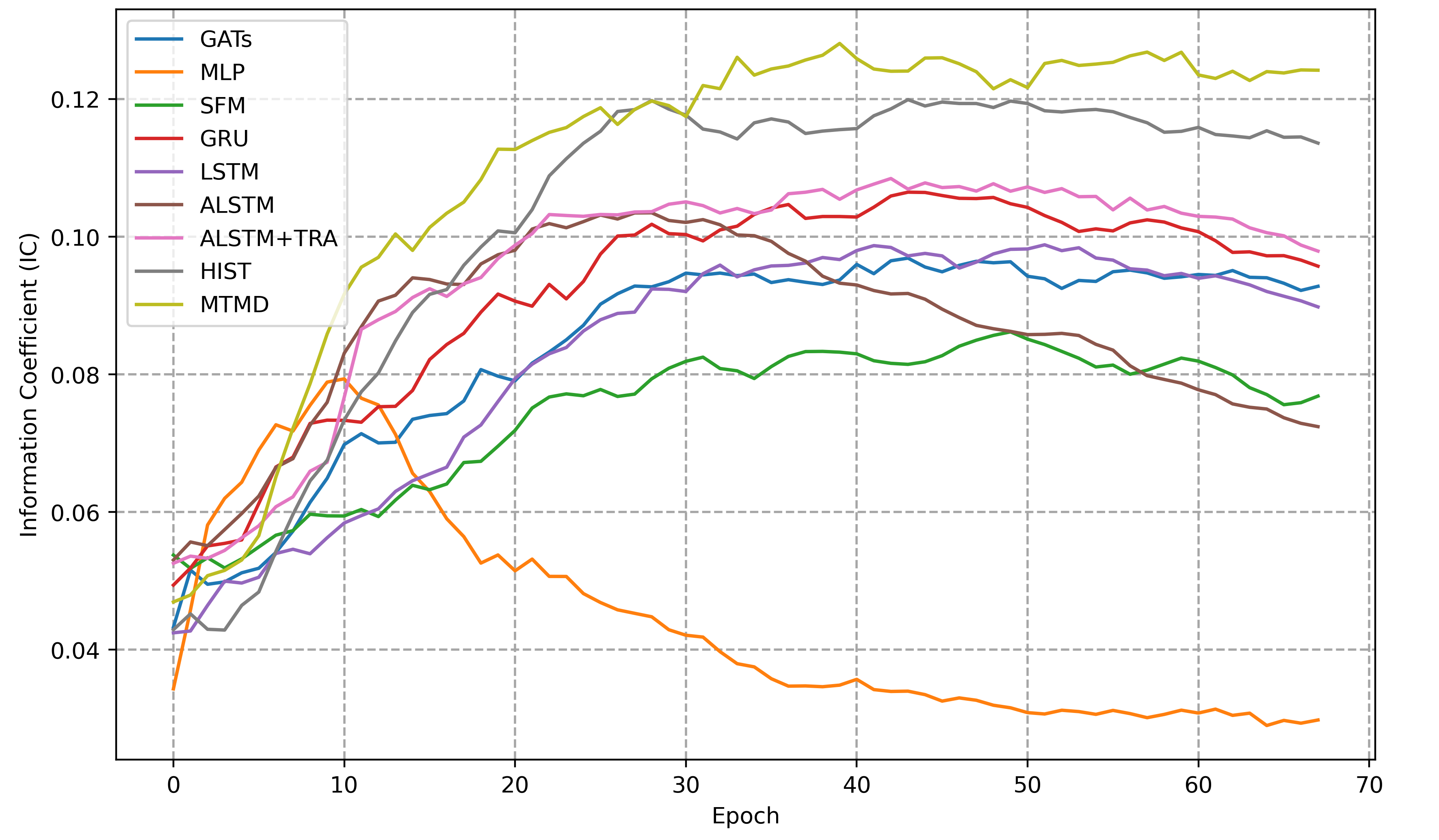
(a) Image of IC on CSI 100

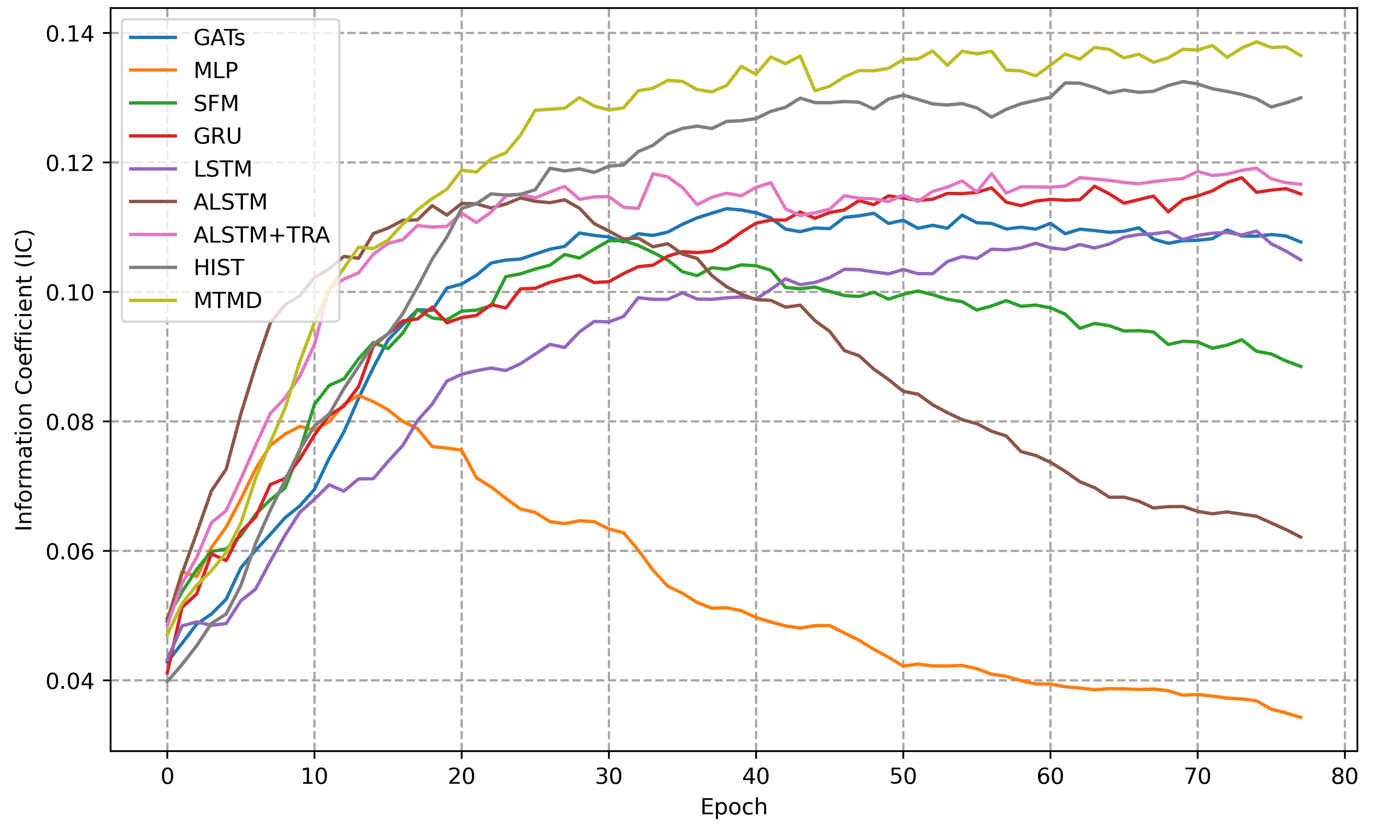
(b) Image of IC on CSI 300

Figure 5: IC on CSI 100 and CSI 300.

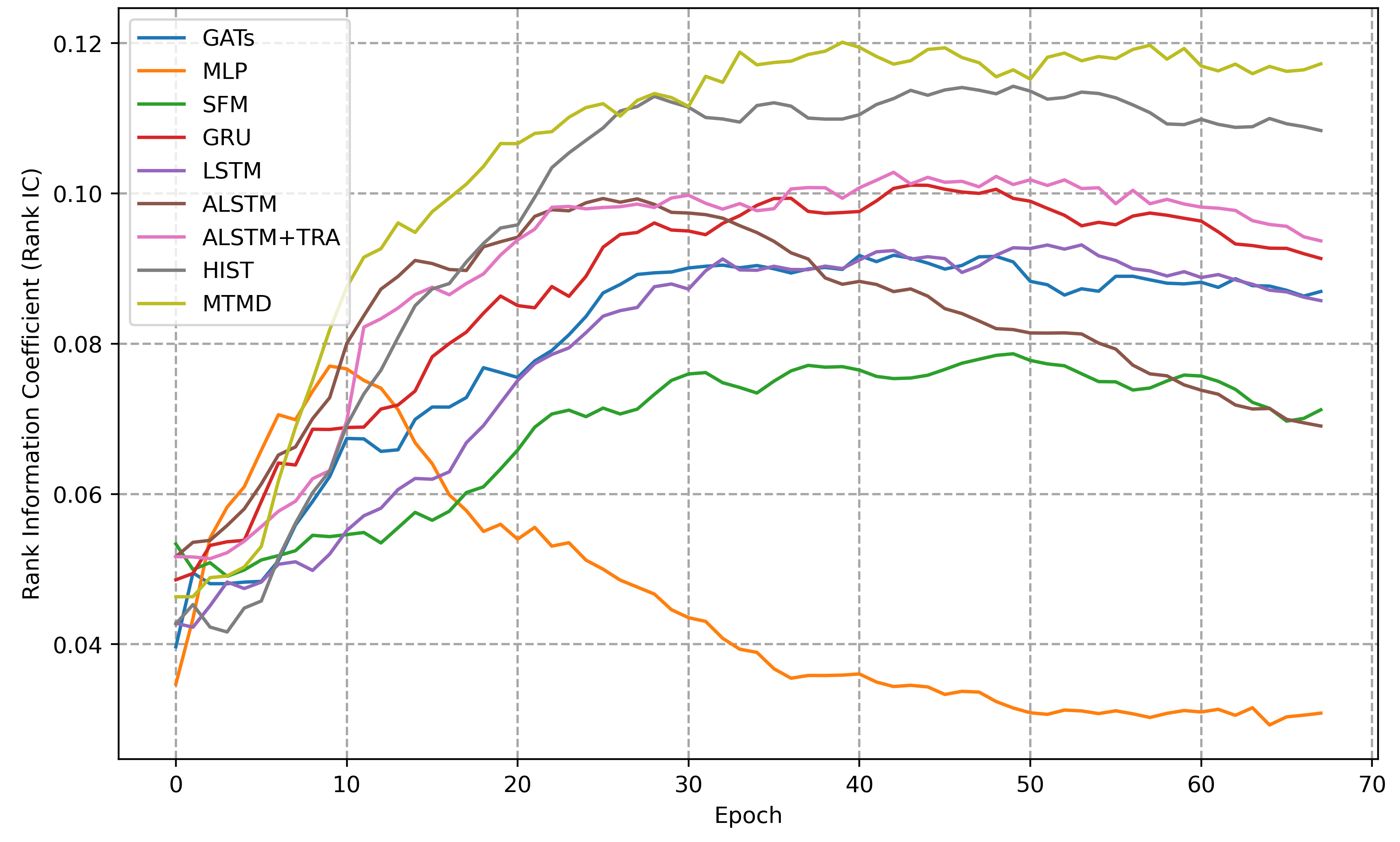
(a) Image of Rank IC on CSI 100

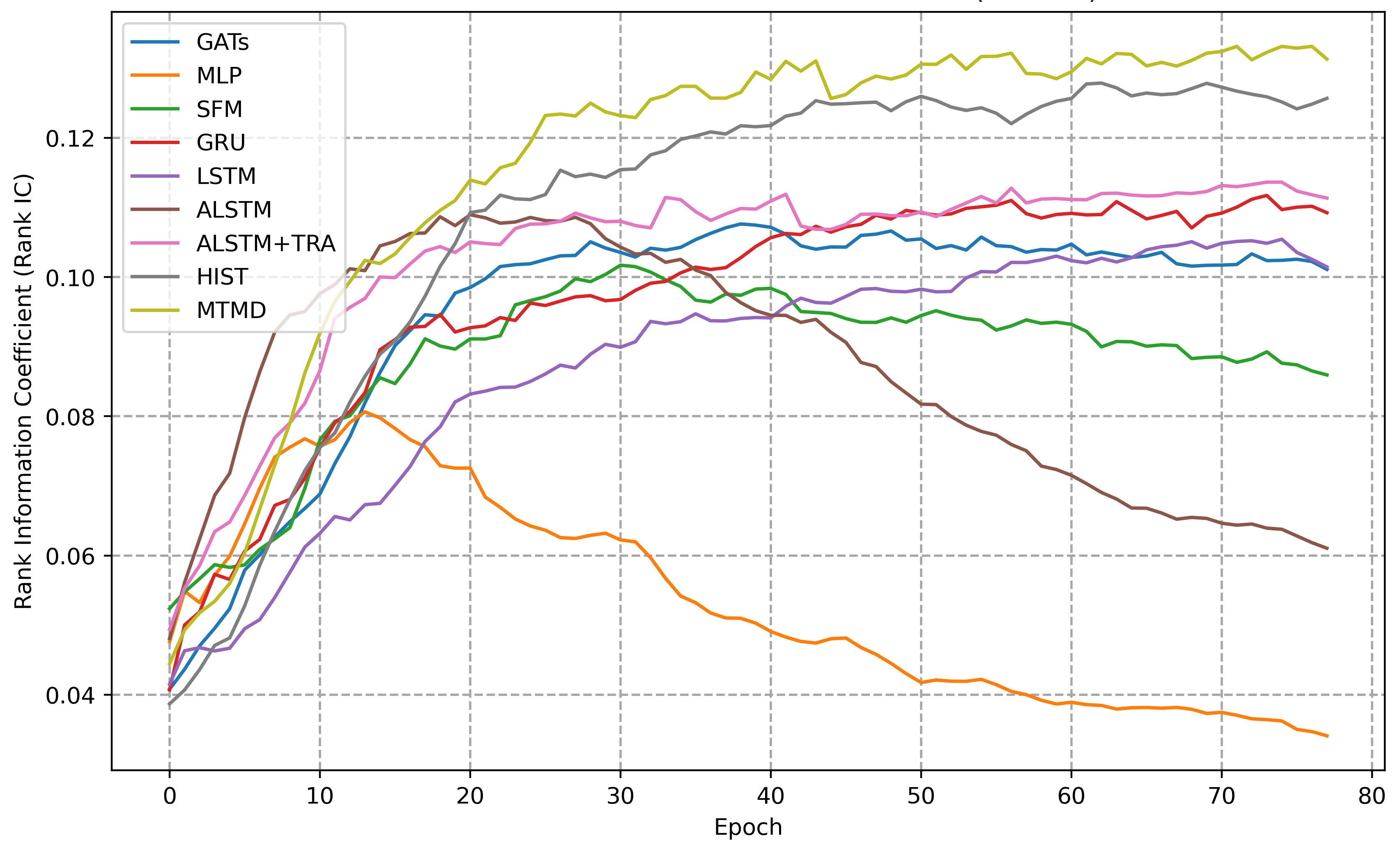
(b) Image of Rank IC on CSI 300

Figure 6: Rank IC on CSI 100 and CSI 300.

Compared with the SFM, ALSTM, ALSTM+TRA, and GRU, which predict stock trends through time series, our framework pays more attention to mining the conceptual features of stocks. The IC of MTMD is 0.008 higher than the best score of ALSTM+TRU on average. This result shows that the concept of stock can better mine the correlation of cross-stock changes to achieve a better forecast performance. Besides, although GATs can also capture the cross-stock connections, it does not study the dynamic correlation between stocks and concepts. However, HIST can more effectively capture the temporary and complicated cross-stock relationship between stocks. Our model is better than that of GATs in IC with an average of 0.112. This means that dynamically associating time features with conceptual features can predict the stock trend more accurately.

The complicated external noise in the market interferes with the learning effect of the model. We believe that a real profit signal can be used as a critical learning feature, and aggregating features can optimize the model at multiple scales. Combining with Figure 5 and Figure 6, we can observe that with the addition of epoch, the IC and Rank IC of most baselines show a gradual decrease after an obvious turning point at the end of the increasing process, while MTMD shows a trend of steady growth. This is a remarkable advantage of our method, which proves that the memory blocks in MTMD prevent them from being wrongly concentrating on the sample bias of each data batch, so that over-fitting can be avoided.

5.3 Ablation Study

Methods	IC ($\uparrow$)	Rank IC ($\uparrow$)	Precision@3 ($\uparrow$)	Precision@5 ($\uparrow$)	Precision@10 ($\uparrow$)	Precision@30 ($\uparrow$)	Memory Block Enabled
HIST	0.120	0.120	61.62	60.89	58.70	56.25	B
MTMD	0.124	0.118	62.86	61.62	59.68	56.27	P
	($4.7e-4$)	($9.4e-4$)	(0.74)	(0.42)	(0.33)	(0.21)
MTMD	0.126	0.120	62.24	61.13	59.86	56.17	H
	($2.0e-3$)	($2.9e-3$)	(0.13)	(0.30)	(0.49)	(0.15)
MTMD	0.128	0.120	61.62	60.89	59.70	56.25	A
	($2.0e-3$)	($1.3e-3$)	(0.66)	(0.53)	(0.08)	(0.19)

Table 3: The results of ablation study on CSI 100. In the memory block enabled, we have B is for baseline, P is for Predefined concept module, H is representative of Hidden concept module, and A means All.

Methods	IC ($\uparrow$)	Rank IC ($\uparrow$)	Precision@3 ($\uparrow$)	Precision@5 ($\uparrow$)	Precision@10 ($\uparrow$)	Precision@30 ($\uparrow$)	Memory Block Enabled
HIST	0.131	0.126	61.60	61.08	60.51	58.79	B
MTMD	0.136	0.132	61.31	61.19	61.12	59.46	P
	($3.0e-3$)	($3.6e-3$)	(0.26)	(0.07)	(0.56)	(0.46)
MTMD	0.137	0.132	62.68	61.65	60.76	59.15	H
	($4.7e-4$)	($4.7e-4$)	(0.64)	(0.28)	(0.22)	(0.27)
MTMD	0.138	0.133	62.51	61.61	60.80	59.25	A
	($1.4e-3$)	($1.3e-3$)	(0.55)	(0.35)	(0.17)	(0.11)

Table 4: The results of ablation study on CSI 300. In the memory block enabled, we have B is for baseline, P is for Predefined concept module, H is representative of Hidden concept module, and A means All.

In the ablation study, we test the significance of the memory block. We adopt HIST as our baseline, which only locally aggregates stock and concept information in each time step. In detail, our framework uses a 2-layer GRU network to encode the time-series features of several target stocks, plus a multi-scale aggregating process with memory block for predefined and hidden concept modules respectively. The experiment results are shown in Table 3 and Table 4. We will then demonstrate the effect of the global aggregation with memory items for each module.

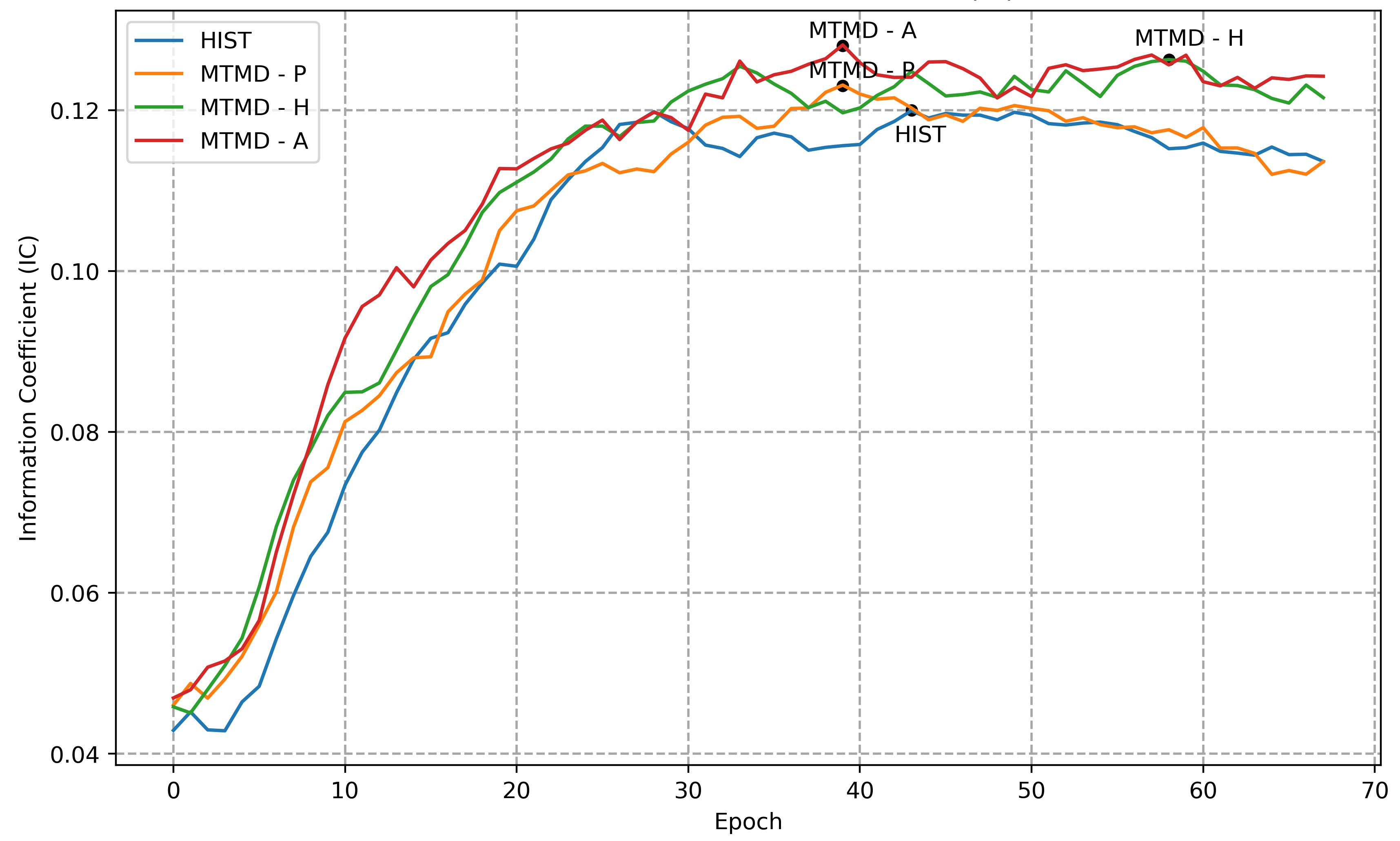
Figure 7: Ablation study of IC on CSI 100.

We first add a memory block to the predefined and hidden concept module separately. Then, when the memory block is applied to the predefined concept module, for test metrics of our model over CSI 100 and CSI 300 dataset, IC is improved by 0.006, Rank IC is improved by 0.006, and Precision@N rises by 0.694 on average. Also, the application of the memory block in the hidden concept module shows that IC is improved by 0.007, and Precision@N rises by 0.763, for the average value of metrics over CSI 100 and CSI 300 dataset. The better results show that information recorded in memory items is conducive to refining locally aggregated stock-concept features.

Moreover, we apply the memory block on these two modules simultaneously with two different sets of memory items for each module. For average metrics over CSI 100 and CSI 300 dataset, IC is improved by 0.009, Rank IC rises by 0.007, and Precision@N increases by 0.437. From Figure 7, it can be observed that the performance is improved more obviously, which means that the simultaneous application of the memory block on these two concept blocks will not cause conflicts, and the overall performance will get promoted.

Therefore, the application of multi-scale aggregation can help the model capture actual profit signals through different time and different inventory levels, which increases the robustness of the model to external noise.

5.4 Visualization of Debiasing

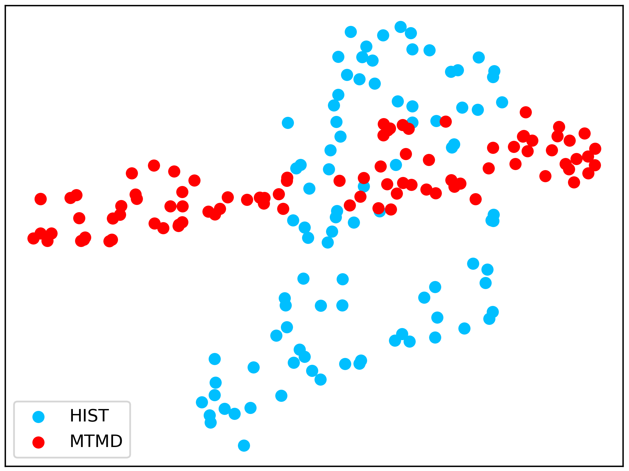
(a) Visualization of global aggregation in hidden concept module.

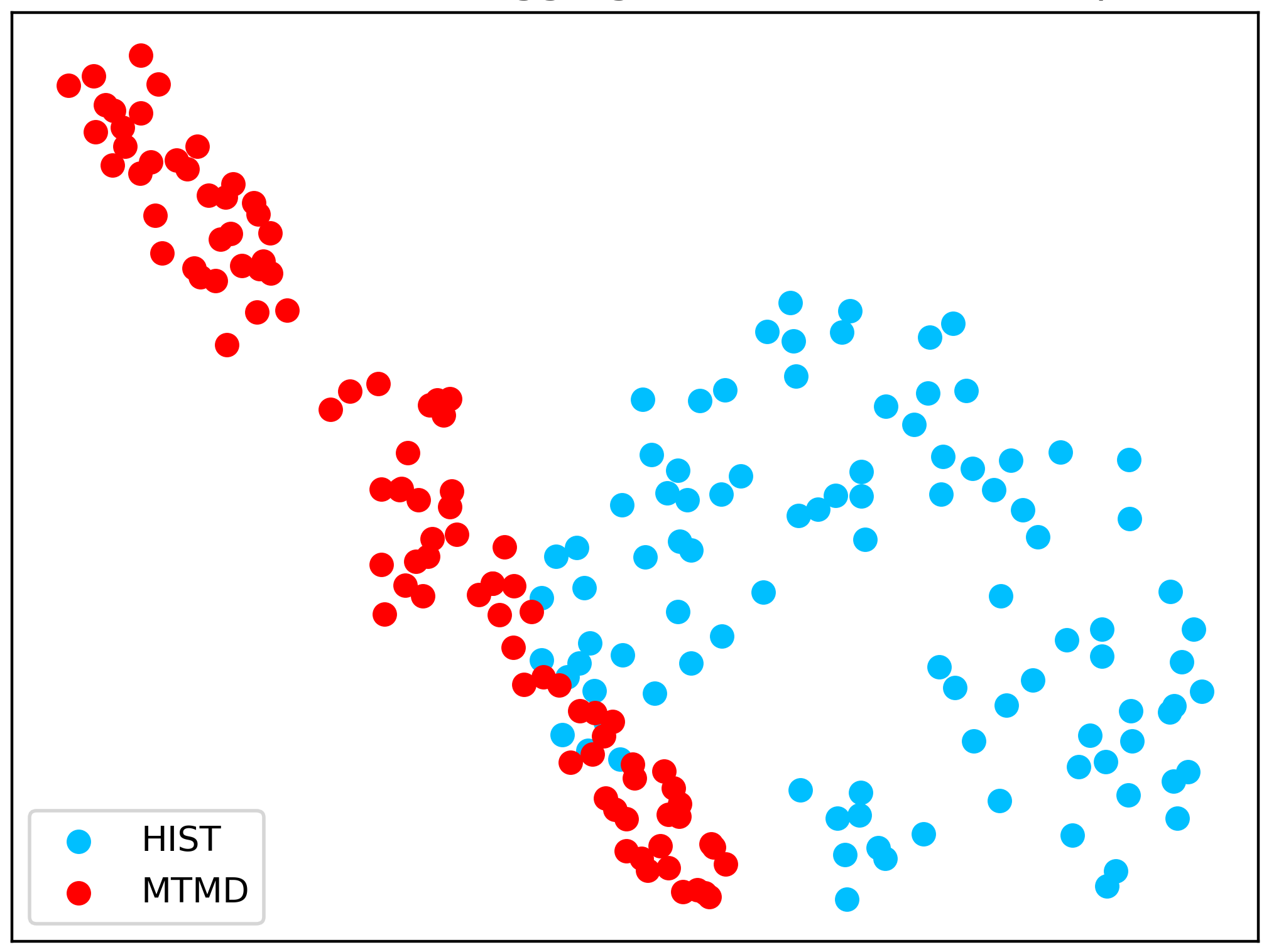
(b) Visualization of global aggregation in predefined concept module.

Figure 8: Visualization of memory matrix with base on t-SNE. And MTMD can capture the real profit signal from the noise more effectively.

We visualize the distribution of MTMD and HIST features based on t-SNE [34] in Figure 8, with samples randomly chosen from CSI 300 dataset. We compare the distribution of stock-concept features of HIST and MTMD to interpret the effect of debias. The distribution of features generated by HIST is sparsely distributed in the dimension space, which means that the feature is noisy, and it is hard for the model to discriminate significant profit signals. With global aggregation performed by the memory block, the features obtained from MTMD are more densely distributed and show an apparent linear pattern. Moreover, the features generated by MTMD present clusters with clear margins indicating the disparity between different kinds of samples, while the features output by HIST scatters in the dimension space without an obvious clustering pattern. Hence, the memory block’s debias effect is proved, making MTMD capture more meaningful information through the noisy stock market.

6 Conclusion

In this paper, we propose a novel time series prediction framework named Multi-scale Temporal Memory Learning and Efficient Debiasing (MTMD). With the help of memory blocks, our MTMD not only effectively aggregates stock-concept information from multi-scale time but also learns the low noise pattern of stock trend based on memorized real profit signals in recorded historical patterns. Moreover, we further enhance the temporal consistency of this model via self-similarity, which is free from time intervals. The experimental results from stock sets CSI 100 and CSI 300 show that our model reaches a new state-of-the-art performance and significantly improves the accuracy of stock trends. Despite our superior performance under real stock sets, markets are constantly changing. In the future, we will deploy our model under a more up-to-date stock market and make it more adaptive to more complex trading environments in real scenarios.

References

- [1] B. Chovancova, M. Dorocakova, V. Malacka, Changes in industrial structure of gdp and stock indices also with regard to the industry 4.0, Business and Economic Horizons (BEH) 14 (1232-2019-761) (2018) 402–414.
- [2] C. R. Chen, J. D. Diltz, Y. Huang, P. P. Lung, Stock and option market divergence in the presence of noisy information, J Bank Financ 35 (8) (2011) 2001–2020.
- [3] W. Jiang, Applications of deep learning in stock market prediction: recent progress, Expert Syst Appl 184 (2021) 115537.
- [4] F. Chen, F. Wu, J. Xu, G. Gao, Q. Ge, X.-Y. Jing, Adaptive deformable convolutional network, Neurocomputing 453 (2021) 853–864.
- [5] T. Chen, J. Guo, W. Wu, Graph representation learning for popularity prediction problem: A survey, Discrete Mathematics, Algorithms and Applications 14 (7) (2022) 2230003.
- [6] Q. Ding, S. Wu, H. Sun, J. Guo, J. Guo, Hierarchical multi-scale gaussian transformer for stock movement prediction, in: IJCAI, 2020, pp. 4640–4646.
- [7] S. Hochreiter, J. Schmidhuber, Long short-term memory, Neural Computation 9 (8) (1997) 1735–1780.
- [8] J. Chung, C. Gulcehre, K. Cho, Y. Bengio, Empirical evaluation of gated recurrent neural networks on sequence modeling, arXiv preprint arXiv:1412.3555 (2014).
- [9] U. Gupta, V. Bhattacharjee, P. S. Bishnu, Stocknet—gru based stock index prediction, Expert Syst Appl 207 (2022) 117986.
- [10] L. Zhang, C. Aggarwal, G.-J. Qi, Stock price prediction via discovering multi-frequency trading patterns, in: Proceedings of the 23rd ACM SIGKDD International Conference on Knowledge Discovery and Data Mining, 2017, pp. 2141–2149.
- [11] W. Xu, W. Liu, L. Wang, Y. Xia, J. Bian, J. Yin, T.-Y. Liu, Hist: A graph-based framework for stock trend forecasting via mining concept-oriented shared information, arXiv preprint arXiv:2110.13716 (2021).
- [12] P. V. G. C. A. Casanova, A. R. P. Lio, Y. Bengio, Graph attention networks, ICLR (2018).
- [13] H. Lin, D. Zhou, W. Liu, J. Bian, Learning multiple stock trading patterns with temporal routing adaptor and optimal transport, KDD ’21, Association for Computing Machinery, 2021, p. 1017–1026.
- [14] Z. Li, D. Yang, L. Zhao, J. Bian, T. Qin, T.-Y. Liu, Individualized indicator for all: Stock-wise technical indicator optimization with stock embedding, in: Proceedings of the 25th ACM SIGKDD International Conference on Knowledge Discovery and Data Mining, 2019, pp. 894–902.
- [15] L. Li, S. Leng, J. Yang, M. Yu, Stock market autoregressive dynamics: a multinational comparative study with quantile regression, Math Probl Eng 2016 (2016).
- [16] A. A. Ariyo, A. O. Adewumi, C. K. Ayo, Stock price prediction using the arima model, in: 2014 UKSim-AMSS 16th International Conference on Computer Modelling and Simulation, IEEE, 2014, pp. 106–112.
- [17] M.-C. Wu, S.-Y. Lin, C.-H. Lin, An effective application of decision tree to stock trading, Expert Syst Appl 31 (2) (2006) 270–274.
- [18] H. Y. Kim, C. H. Won, Forecasting the volatility of stock price index: A hybrid model integrating lstm with multiple garch-type models, Expert Syst Appl 103 (2018) 25–37.
- [19] Z. Jin, Y. Yang, Y. Liu, Stock closing price prediction based on sentiment analysis and lstm, Neural Comput Appl 32 (13) (2020) 9713–9729.
- [20] M. Ballings, D. Van den Poel, N. Hespeels, R. Gryp, Evaluating multiple classifiers for stock price direction prediction, Expert Syst Appl 42 (20) (2015) 7046–7056.
- [21] T. Le, B. Vo, H. Fujita, N.-T. Nguyen, S. W. Baik, A fast and accurate approach for bankruptcy forecasting using squared logistics loss with gpu-based extreme gradient boosting, Inform Sciences 494 (2019) 294–310.
- [22] K.-j. Kim, I. Han, Genetic algorithms approach to feature discretization in artificial neural networks for the prediction of stock price index, Expert Syst Appl 19 (2) (2000) 125–132.
- [23] C.-H. Cheng, T.-L. Chen, L.-Y. Wei, A hybrid model based on rough sets theory and genetic algorithms for stock price forecasting, Inform Sciences 180 (9) (2010) 1610–1629.
- [24] R. Aguilar-Rivera, M. Valenzuela-Rendón, J. Rodríguez-Ortiz, Genetic algorithms and darwinian approaches in financial applications: A survey, Expert Syst Appl 42 (21) (2015) 7684–7697.
- [25] C. Xiaoning, W. Shang, F. Jiang, W. Shouyang, Stock index forecasting by hidden markov models with trends recognition, in: 2019 IEEE International Conference on Big Data (BigData), IEEE, 2019, pp. 5292–5297.
- [26] K. Chen, Y. Zhou, F. Dai, A lstm-based method for stock returns prediction: A case study of china stock market, in: 2015 IEEE International Conference on Big Data (BigData), IEEE, 2015, pp. 2823–2824.
- [27] D. M. Nelson, A. C. Pereira, R. A. De Oliveira, Stock market’s price movement prediction with lstm neural networks, in: 2017 International Joint Conference on Neural Networks (IJCNN), IEEE, 2017, pp. 1419–1426.
- [28] H. Xu, L. Chai, Z. Luo, S. Li, Stock movement prediction via gated recurrent unit network based on reinforcement learning with incorporated attention mechanisms, Neurocomputing 467 (2022) 214–228.
- [29] F. Feng, H. Chen, X. He, J. Ding, M. Sun, T.-S. Chua, Enhancing stock movement prediction with adversarial training, IJCAI (2019) 5843–5849.
- [30] C. Xu, H. Huang, X. Ying, J. Gao, Z. Li, P. Zhang, J. Xiao, J. Zhang, J. Luo, Hgnn: Hierarchical graph neural network for predicting the classification of price-limit-hitting stocks, Inform Sciences 607 (2022) 783–798.
- [31] R. Kim, C. H. So, M. Jeong, S. Lee, J. Kim, J. Kang, Hats: A hierarchical graph attention network for stock movement prediction, arXiv preprint arXiv:1908.07999 (2019).
- [32] X. Yang, W. Liu, D. Zhou, J. Bian, T.-Y. Liu, Qlib: An ai-oriented quantitative investment platform, arXiv preprint arXiv:2009.11189 (2020).
- [33] A. Paszke, S. Gross, F. Massa, A. Lerer, J. Bradbury, G. Chanan, T. Killeen, Z. Lin, N. Gimelshein, L. Antiga, et al., Pytorch: An imperative style, high-performance deep learning library, Advances in neural information processing systems 32 (2019).
- [34] L. van der Maaten, G. Hinton, Visualizing data using t-sne, J Mach Learn Res 9 (86) (2008) 2579–2605.