GFPose: Learning 3D Human Pose Prior with Gradient Fields

Abstract

Learning 3D human pose prior is essential to human-centered AI. Here, we present GFPose, a versatile framework to model plausible 3D human poses for various applications. At the core of GFPose is a time-dependent score network, which estimates the gradient on each body joint and progressively denoises the perturbed 3D human pose to match a given task specification. During the denoising process, GFPose implicitly incorporates pose priors in gradients and unifies various discriminative and generative tasks in an elegant framework. Despite the simplicity, GFPose demonstrates great potential in several downstream tasks. Our experiments empirically show that 1) as a multi-hypothesis pose estimator, GFPose outperforms existing SOTAs by 20% on Human3.6M dataset. 2) as a single-hypothesis pose estimator, GFPose achieves comparable results to deterministic SOTAs, even with a vanilla backbone. 3) GFPose is able to produce diverse and realistic samples in pose denoising, completion and generation tasks.

1 Introduction

Modeling 3D human pose is a fundamental problem in human-centered applications, e.g. augmented reality [31, 40], virtual reality [1, 67, 39], and human-robot collaboration [9, 15, 33]. Considering the biomechanical constraints, natural human postures lie on a low-dimensional manifold of the physical space. Learning a good prior distribution over the valid human poses not only helps to discriminate the infeasible ones but also enables sampling of rich and diverse human poses. The learned prior has a wide spectrum of use cases with regard to recovering the 3D human pose under different conditions, e.g., monocular images with depth ambiguities and occlusions [8, 60], inertial measurement unit (IMU) signals with noises [70], or even partial sensor inputs [63, 22].

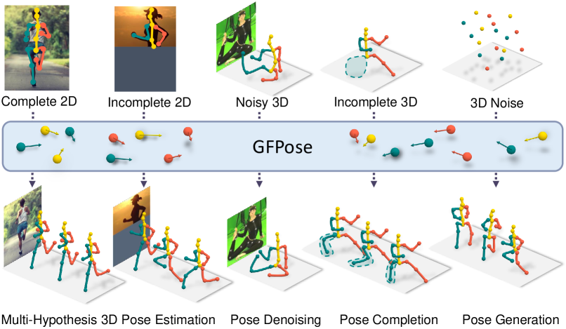
Figure 1: GFPose learns the 3D human pose prior from 3D human pose datasets and represents it as gradient fields for various applications, e.g., multi-hypothesis 3D pose estimation from 2D keypoints, correcting noisy poses, completing missing joints, and generating natural poses from noise.

Previous works explore different ways to model human pose priors. Pioneers [16, 26] attempt to explicitly build joint-angle limits based on biomechanics. Unfortunately, the complete configuration of pose-dependent joint-angle constraints for the full body is unknown. With the recent advances in machine learning, a rising line of works seek to learn the human pose priors from data. Representative methods include modeling the distribution of plausible poses with GMM[5], VAE[43], GAN[12] or neural implicit functions[58]. These methods learn an independent probabilistic model or energy function to characterize the data distribution $p_{data}(\mathbf{x})$. They usually require additional optimization process to introduce specific task constraints when applied to downstream tasks. Therefore extra efforts such as balancing prior terms and different task objectives are inevitable. Some methods jointly learn the pose priors and downstream tasks via adversarial training [23, 25] or explicit task conditions [32, 47, 45] $p_{data}(\mathbf{x}|\mathbf{c})$. These methods seamlessly integrate priors into learning-based frameworks, but limit their use to a single given task.

In this work, we take a new perspective to learn a versatile 3D human pose prior model for general purposes. Different from previous works that directly model the plausible pose distribution $p_{data}(\mathbf{x})$, we learn the score (gradient of a log-likelihood) of a task conditional distribution $\nabla_{\mathbf{x}}\log p_{data}(\mathbf{x}|\mathbf{c})$, where $\mathbf{c}$ is the task-specific condition, e.g., for 3D human pose estimation, $\mathbf{c}$ could be 2D images or detected 2D poses. $\mathbf{x}$ represents plausible 3D human poses. In this way, we can jointly encode the human pose prior and the task specification into the score, instead of considering the learned prior model as an ad-hoc plugin as in an optimization process. To further enhance the flexibility and versatility, we introduce a condition masking strategy, where task conditions are randomly masked to varying degrees during training. Different masks correspond to different task specifications. Thus we can handle various pose-related tasks in a unified learning-based framework.

We present GFPose, a general framework for pose-related tasks. GFPose learns a time-dependent score network $\mathbf{s}_{\theta}(\mathbf{x},t|\mathbf{c})$ to approximate $\nabla_{\mathbf{x}}\log p_{data}(\mathbf{x}|\mathbf{c})$ on a large scale 3D human pose dataset [19] via Denoising Score Matching (DSM) [59, 18, 54, 52, 53, 56, 51]. Specifically, for any valid human pose $\mathbf{x}\in\mathbb{R}^{J\times 3}$ in Euclidean space, we sample a time-dependent noise $\mathbf{z}(t)$ from a prior distribution, perturb $\mathbf{x}$ to get the noisy pose $\mathbf{\widetilde{x}}$, then train $\mathbf{s}_{\theta}(\mathbf{\widetilde{x}},t|\mathbf{c})$ to learn the score towards the valid pose. Intuitively, the score points in the direction of increasing pose plausibility. To handle a wider range of downstream tasks, we adopt a hierarchical condition masking strategy in training. Concretely, we randomly mask out the task condition $\mathbf{c}$ by sampling masks from a hierarchy of candidate masks. The candidate masks cover different levels of randomness, including human level, body part level, and joint level. This helps the model to build the spatial relation between different body joints and parts, and enables GFPose directly applicable to different task settings at test time (Figure 1), e.g., recovering 3D pose from severe occlusions when $\mathbf{c}$ is partially masked 2D pose or unconditional pose generation when $\mathbf{c}$ is fully masked ($\mathbf{c}=\O$).

We evaluate GFPose on various downstream tasks, including monocular 3D human pose estimation, pose denoising, completion, and generation. Empirical results on the H3.6M benchmark [19] show that: 1) GFPose outperforms SOTA in both multi-hypothesis and single-hypothesis pose estimation tasks [60] and demonstrates stronger robustness to severe occlusions in pose completion [28]. Notably, under the single-hypothesis setting, GFPose can achieve comparable pose estimation performance to previous deterministic SOTA methods [68, 11, 44] that learns one-to-one mapping. To the best of our knowledge, this is for the first time that a probabilistic model can achieve such performance. 2) As a pose generator, GFPose can produce diverse and realistic samples that can be used to augment existing datasets. We summarize our contributions as follows:

• We introduce GFPose, a novel score-based generative framework to model plausible 3D human poses.

• We design a hierarchical condition masking strategy to enhance the versatility of GFPose and make it directly applicable to various downstream tasks.

• We demonstrate that GFPose outperforms SOTA on multiple tasks under a simple unified framework.

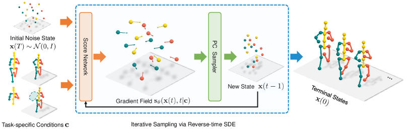
Figure 2: Inference pipeline of GFPose. For a downstream task specified by condition $\mathbf{c}$, we generate terminal states $\mathbf{x}(0)$ from initial noise states $\mathbf{x}(T)\sim\mathcal{N}(0,I)$ via a reverse-time Stochastic Differential Equation (RSDE). $T$ denotes the start time of RSDE. This process is simulated by a Predictor-Corrector sampler[56]. At each time step $t$, the time-dependent score network $\mathbf{s}_{\theta}(\mathbf{x}(t),t|\mathbf{c})$ outputs gradient fields that ‘pull’ the pose to be more valid and faithful to the task condition $\mathbf{c}$.

2 Related Work

2.1 Human Pose Priors

We roughly group previous works on learning 3D human pose priors into two categories. The first line of works learns task-independent pose priors, i.e.they learn the unconditional distribution $p_{data}(\mathbf{x})$ of plausible poses. These approaches usually involve time-consuming optimization process to introduce task-specific constraints when applying the learned priors to different downstream tasks. Akheter et al.  [2] learns the pose-dependent joint-angle limits directly. SMPLify [5] fits a mixture of Gaussians to motion capture (mocap) data. VAE-based methods such as VPoser [43] map the 3D poses to a compact representation space and can be used to generate valid poses. GAN-based methods[12] learn adversarial priors by discriminating the generated poses from the real poses. Most recently, Pose-NDF [58] proposes to model the plausible pose manifolds with a neural implicit function. The second line of works focuses on task-aware priors. They learn the conditional priors $p_{data}(\mathbf{x}|\mathbf{c})$ under specific task constraints. MVAE[32] and HuMoR [47] employ autoregressive conditional VAE to learn plausible pose trajectories given the historical state. ACTOR [45] learns an action-conditioned variational prior using Transformer VAE. HMR [23] and VIBE [25] jointly train the model with the adversarial prior loss and pose reconstruction loss. In this paper, we explore a novel score-based framework to model plausible human poses. Our method jointly learns the task-independent and various task-aware priors via a hierarchical condition masking strategy. Thus it is native and directly applicable to multiple downstream tasks without involving extra optimization steps.

2.2 3D Human Pose Estimation

Estimating the 3D human pose from a monocular RGB image is a fundamental yet unresolved problem in computer vision. The common two-stage practice is estimating the 2D pose with an off-the-shelf estimator first, then lifting it to 3D, which improves the model generalization. Most existing methods directly learn the 2D-to-3D mapping via various architecture designs [37, 10, 66, 71, 36]. Nonetheless, solving the 2D-to-3D mapping is intrinsically an ill-posed problem as infinite solutions suffice without extra constraints. Therefore, formulating and learning 3D human pose estimation as a one-to-one mapping fails to express the ambiguity and inevitably suffers from degraded precision [13, 14]. To this end, Li et al. [28] propose a multimodal mixture density network to learn the plausible pose distribution instead of the one-to-one mapping. Jahangiri et al. [20] design a compositional generative model to generate multiple 3D hypotheses from 2D joint detections. Sharma et al. [49] first sample plausible candidates with a conditional variational autoencoder, then use ordinal relations to filter and fuse the candidates. [27, 61, 46] employs normalizing flows to model the distribution of plausible human poses. Li et al. [30] use a transformer to learn the spatial-temporal representation of multiple hypotheses. We show that GFPose is a suitable solution for multi-hypothesis 3D human pose estimation, and is able to handle severe occlusions by producing plausible hypotheses.

2.3 Score-Based Generative Model

The score-based generative model aims at estimating the gradient of the log-likelihood of a given data distribution [59, 18, 54, 52, 53, 56, 51]. To improve the scalability of the score-based generative model, [54] introduces a sliced score-matching objective that projects the scores onto random vectors before comparing them. Song et al. introduce annealed training for denoising score matching [52] and several improved training techniques [53]. They further extend the discrete levels of annealed score matching to a continuous diffusion process and show promising results on image generation [56]. These recent advances promote the wide application of the score-based generative model in different fields, such as object rearrangement [64], medical imaging [55], point cloud generation [6], molecular conformation generation [50], scene graph generation [57], point cloud denoising [35], offline reinforcement learning [21], and depth completion [48]. Inspired by these promising results, we seek to develop a score-based framework to model plausible 3D human poses. To the best of our knowledge, our method is the first to explore score-based generative models for learning 3D human pose priors.

3 Revisiting Denoising Score Matching

Given samples $\{\mathbf{x}_{i}\}_{i=1}^{N}$ from an unknown data distribution $\{\mathbf{x}_{i}\sim p_{data}(\mathbf{x})\}$, the score-based generative model aims at learning a score function to approximate $\nabla_{\mathbf{x}}\log p_{data}(\mathbf{x})$ via a score network $\mathbf{s}_{\theta}(\mathbf{x}):\mathbb{R}^{|\mathcal{X}|}\rightarrow\mathbb{R}^{|\mathcal{X}|}$.

$$\mathcal{L}(\theta)=\frac{1}{2}\mathbb{E}_{p_{data}}\left[||\mathbf{s}_{\theta}(\mathbf{x})-\nabla_{\mathbf{x}}\log p_{data}(\mathbf{x})||^{2}_{2}\right].$$ (1)

During the test phase, a new sample is generated by Markov chain Monte Carlo (MCMC) sampling, e.g., Langevin Dynamics (LD). Given a step size $\epsilon>0$, an initial point $\tilde{\mathbf{x}}_{0}$ and a Gaussian noise $\mathbf{z}_{t}\sim\mathcal{N}(0,I)$, LD can be written as:

$$\tilde{\mathbf{x}}_{t}=\tilde{\mathbf{x}}_{t-1}+\frac{\epsilon}{2}\nabla_{\mathbf{x}}\log p_{data}(\tilde{\mathbf{x}}_{t-1})+\sqrt{\epsilon}\mathbf{z}_{t}.$$ (2)

When $\epsilon\rightarrow 0$ and $t\rightarrow\infty$, the $\tilde{\mathbf{x}}_{t}$ becomes an exact sample from $p_{data}(\mathbf{x})$ under some regularity conditions [62].

However, the vanilla objective of score-matching in Eq. 1 is intractable, since $p_{data}(\mathbf{x})$ is unknown. To this end, the Denoising Score-Matching (DSM) [59] proposes a tractable objective by pre-specifying a noise distribution $q_{\sigma}(\widetilde{\mathbf{x}}|\mathbf{x})$, e.g., $\mathcal{N}(0,\sigma^{2}I)$, and train a score network to denoise the perturbed data samples:

$$\mathcal{L}(\theta)=\mathbb{E}_{\widetilde{\mathbf{x}}\sim q_{\sigma},\mathbf{x}\sim p_{data}}\left[||\mathbf{s}_{\theta}(\widetilde{\mathbf{x}})-\nabla_{\widetilde{\mathbf{x}}}\log q_{\sigma}(\widetilde{\mathbf{x}}|\mathbf{x})||^{2}_{2}\right]$$ (3)

where $\nabla_{\widetilde{\mathbf{x}}}\log q_{\sigma}(\widetilde{\mathbf{x}}|\mathbf{x})=\frac{1}{\sigma^{2}}(\mathbf{x}-\widetilde{\mathbf{x}})$ are tractable for the Gaussian kernel. DSM guarantees that the optimal score network holds $\mathbf{s}_{\theta}^{*}(\mathbf{x})=\nabla_{\mathbf{x}}\log p_{data}(\mathbf{x})$ for almost all $\mathbf{x}$.

4 Method

4.1 Problem Statement

We seek to model 3D human pose priors under different task conditions $p_{data}(\mathbf{x}|\mathbf{c})$ by estimating $\nabla_{\mathbf{x}}\log p_{data}(\mathbf{x}|\mathbf{c})$ from a paired dataset $\{(\mathbf{x},\mathbf{c})\}^{N}$, where $\mathbf{x}\in\mathbb{R}^{J\times 3}$ represents plausible 3D human poses and $\mathbf{c}$ denotes different task conditions. In this work, we consider $\mathbf{c}$ to be 2D poses ($\mathbf{c}\in\mathbb{R}^{J\times 2}$) for monocular 3D human pose estimation tasks; 3D poses ($\mathbf{c}\in\mathbb{R}^{J\times 3}$) for 3D pose completion; $\O$ for pose generation and denoising. (elaborate in Section 5) We further introduce a condition masking strategy to unify different task conditions and empower the model to handle occlusions. Notably, this formulation does not limit to the choices used in this paper. In general, $\mathbf{c}$ can be any form of observation, e.g., image features or human silhouettes for recovering 3D poses from the image domain. $\mathbf{x}$ could also be different forms of 3D representation, e.g., joint rotation in SMPL [34]. With a learned prior model, different downstream tasks can be formulated as a unified generative problem, i.e., generate new samples from $p_{data}(\mathbf{x}|\mathbf{c})$.

4.2 Learning Pose Prior with Gradient Fields

We adopt an extension [56] of Denoising Score Matching (DSM) [59] to learn the score $\nabla_{\mathbf{x}}\log p_{data}(\mathbf{x}|\mathbf{c})$ and sample plausible poses from the data distribution $p_{data}(\mathbf{x}|\mathbf{c})$. The whole framework consists of a forward diffusion process and a reverse sampling process: (1) The forward diffusion process perturbs the 3D human poses from the data distribution to a predefined prior distribution, e.g., Gaussian distribution. (2) The reverse process samples from the prior distribution and reverse the diffusion process to get a plausible pose from the data distribution.

Perturb Poses via SDE Following [56], we construct a time-dependent diffusion process $\{\mathbf{x}(t)\}^{T}_{t=0}$ indexed by a continuous time variable $t\in[0,T]$. $\mathbf{x}(0)\sim p_{0}$ comes from the data distribution. $\mathbf{x}(T)\sim p_{T}$ comes from the diffused prior distribution. As $t$ grows from $0$ to $T$, we gradually perturb the poses with growing levels of noise. The perturbation procedure traces a continuous-time stochastic process and can be modeled by the solution to an It$\hat{o}$ SDE:

$$d\mathbf{x}=\mathbf{f}(\mathbf{x},t)dt+g(t)d\mathbf{w}$$ (4)

where $\mathbf{f}(\cdot,t):\mathbb{R}^{d}\to\mathbb{R}^{d}$ is called the drift coefficient, $g(t)\in\mathbb{R}$ is called the diffusion coefficient of $\mathbf{x}(t)$. $dt$ represents infinitesimal time step. $\mathbf{w}$ is the Brownian motion, and $d\mathbf{w}$ can be seen as infinitesimal white noise. We have various designs of SDEs to perturb the pose $\mathbf{x}$, i.e., different choices of $\mathbf{f}(\cdot,t)$ and $g(t)$. In this work, we use the subVP SDE proposed in [56], which perturbs any human poses $\mathbf{x}(0)$ to a Gaussian distribution $p_{T}$.

Sample Poses via Reverse-Time SDE If we reverse the perturbation process, we can get a pose sample $\mathbf{x}(0)\sim p_{0}$ from a Gaussian noise $\mathbf{x}(T)\sim p_{T}$. According to [3, 56], the reverse is another diffusion process described by the reverse-time SDE (RSDE):

$$d\mathbf{x}=[\mathbf{f}(\mathbf{x},t)-g^{2}(t)\nabla_{\mathbf{x}}\log p_{t}(\mathbf{x}|\mathbf{c})]dt+g(t)d\bar{\mathbf{w}}$$ (5)

where $t$ starts from $T$ and flows back to $0$. $dt$ here represents negative time step and $\bar{\mathbf{w}}$ denotes Brownian motion at reverse time. In order to simulate Eq. 5, we need to know $\nabla_{\mathbf{x}}\log p_{t}(\mathbf{x}|\mathbf{c})$ for all $t$. We train a neural network to estimate it.

Train Score Estimation Network According to Eq. 3, we train a time-dependent score network $\mathbf{s}_{\theta}(\mathbf{x},t|\mathbf{c}):\mathcal{X}\times\mathbb{R}^{+}\times\mathcal{C}\rightarrow\mathcal{X}$ to estimate $\nabla_{\mathbf{x}}\log p_{t}(\mathbf{x}|\mathbf{c})$ for all $t$, where $\mathcal{C}$ denotes the condition space. The objective can be written as:

$$\mathbb{E}_{t\sim\mathcal{U}(0,T)}\{\lambda(t)\mathbb{E}_{\mathbf{x}(0)\sim p_{0}(\mathbf{x}|\mathbf{c}),\mathbf{x}(t)\sim p_{0t}(\mathbf{x}(t)|\mathbf{x}(0),\mathbf{c})}$$ (6)

$$[\|\mathbf{s}_{\theta}(\mathbf{x}(t),t|\mathbf{c})-\nabla_{\mathbf{x}(t)}\log p_{0t}(\mathbf{x}(t)\mid\mathbf{x}(0),\mathbf{c})\|_{2}^{2}]\}$$

where $t$ is uniformly sampled over $[0,T]$. $\lambda(t)$ is a weighting term. $p_{0t}$ denotes the perturbation kernel. Due to the choice of subVP SDE, we can get a closed form of $p_{0t}$2. Thus, we can get a tractable objective of Eq. 6.

Given a well-trained score network $\mathbf{s}_{\theta}(\mathbf{x},t|\mathbf{c})$, we can iterate over Eq. 5 to sample poses from $p_{data}(\mathbf{x}|\mathbf{c})$ as illustrated in Fig. 2. At each time step $t$, the network takes the current pose $\mathbf{x}(t)$, time step $t$ and task condition $\mathbf{c}$ as input and outputs the gradient $\nabla_{\mathbf{x}(t)}\log p_{t}(\mathbf{x}(t)|\mathbf{c})$ that intuitively guides the current pose to be more feasible to the task condition. To improve the sample quality, we simulate the reverse-time SDE via a Predictor-Corrector (PC) sampler [56]2.

4.3 Masked Condition for Versatility

To handle different applications and enhance the versatility, we design a hierarchical masking strategy to randomly mask the task condition $\mathbf{c}$ while training $\mathbf{s}_{\theta}(\mathbf{x},t|\mathbf{c})$. Concretely, we design a 3-level mask hierarchy to deal with human-pose-related tasks: $M=M_{human}\odot M_{part}\odot M_{joint}$. $M_{human}$ indicates whether a condition $\mathbf{c}$ is fully masked out with probability $p_{h}$ (result in $\O$ for unconditional pose prior $p_{data}(\mathbf{x}|\O)$). $M_{part}$ indicates whether each human body part in $\mathbf{c}$ should be masked out with probability $p_{p}$. It facilitates recovery from occluded human body parts in the pose completion task. Practically, we think of humans as consisting of 5 body parts: 2 legs, 2 arms, torso. $M_{joint}$ indicates if we should randomly mask each human joint independently with probability $p_{j}$. This facilitates recovery from occluded human body joints in the pose completion task. We augment our model $\mathbf{s}_{\theta}(\mathbf{x},t|\mathbf{c})$ with $\mathbf{c}=M\odot\mathbf{c}$ during training.

5 Experiments

In this section, we first provide summaries of the datasets and evaluation metrics we use and then elaborate on the implementation details. Then, we demonstrate the effectiveness and generalizability of GFPose under different problem settings, including pose estimation, pose denoising, pose completion, and pose generation. Moreover, we ablate design factors of GFPose in the 3D human pose estimation task for in-depth analysis.

5.1 Datasets and Evaluation Metrics

Human3.6M (H3.6M) [19]

is a large-scale dataset for 3D human pose estimation, which consists of 3.6 million poses and corresponding images featuring 11 actors performing 15 daily activities from 4 camera views. Following the standard protocols, the models are trained on subjects $1$, $5$, $6$, $7$, $8$ and tested on subjects $9$, $11$. We evaluate the performance with the Mean Per Joint Position Error (MPJPE) measure following two protocols. Protocol #1 computes the MPJPE between the ground-truth (GT) and the estimated 3D joint coordinates after aligning their root (mid-hip) joints. Protocol #2 computes MPJPE after applying a rigid alignment between GT and prediction. For multi-hypothesis estimation, we follow the previous works [20, 28, 29, 60] to compute the MPJPE between the ground truth and the best 3D hypothesis generated by our model, denoted as minMPJPE.

MPI-INF-3DHP (3DHP) [38]

features more complex cases including indoor scenes, green screen indoor scenes, and outdoor scenes. We directly apply our model, which is trained on the H3.6M dataset, to 3DHP without extra finetuning to evaluate its generalization capability following the convention. We report the Percentage of Correctly estimated Keypoints (PCK) with a threshold of $150$ mm.

5.2 Implementation Details

We use Stacked Hourglass network (SH) [41] as our 2D human pose estimator for any downstream tasks that require 2D pose conditions, e.g., 3D human pose estimation. SH is pretrained on the MPII dataset [4] and finetuned on the H3.6M dataset [19]. We set the time range of subVP SDE [56] to $t\in[0,1.0]$. To better demonstrate the effectiveness of the proposed pipeline, we choose a vanilla fully connected network [37] as the backbone of our score network. While many recent works take well-designed GNNs [10, 69] and Transformers [30, 72] as their backbone to enhance performance, we show GFPose can exhibit competitive results with a simple backbone. We use 2 residual blocks and set the hidden dimension of our score network to 1024 as in [37]. We adopt exponential moving average with a ratio of 0.9999 and a quick warm start to stabilize the training process as suggested by [52]. We do not use additional data augmentation techniques commonly used in previous works, e.g., additional inputs (2d detection confidence, heatmaps, ordinal labels) and augmentation (horizontal flipping). We train GFpose with a batch size of 1000, learning rate $2e-4$, and Adam optimizer[24]. Note that we can train a unified model for all downstream applications with a mixed condition masking strategy (when training together with 3D pose conditions, we add zeros to the last dimension of the 2D poses for a unified condition representation) or train separate models for each task with independent conditions and masking strategies. In the main paper, we report the performance of independently trained models, which slightly improve over the unified model on each task. We use “HPJ-xxx” to denote the masking strategy used during training. E.g., HPJ-010 means only the part level mask is activated with probability $0.1$. We use “T” to denote the probability $1.0$. Please refer to the Supplementary for detailed settings of each task and results of the unified model.

5.3 Monocular 3D Pose Estimation (2D$\rightarrow$3D)

5.3.1 Multi-Hypothesis

Protocol #1	Dire.	Disc.	Eat	Greet	Phone	Photo	Pose	Purch.	Sit	SitD	Smoke	Wait	WalkD	Walk	WalkT	Avg
Martinez et al.  [37] $(S=1)$	51.8	56.2	58.1	59.0	69.5	78.4	55.2	58.1	74.0	94.6	62.3	59.1	65.1	49.5	52.4	62.9
Li et al.  [29] $(S=10)$	62.0	69.7	64.3	73.6	75.1	84.8	68.7	75.0	81.2	104.3	70.2	72.0	75.0	67.0	69.0	73.9
Li et al.  [28] $(S=5)$	43.8	48.6	49.1	49.8	57.6	61.5	45.9	48.3	62.0	73.4	54.8	50.6	56.0	43.4	45.5	52.7
Oikarinen et al.  [42] $(S=200)$	40.0	43.2	41.0	43.4	50.0	53.6	40.1	41.4	52.6	67.3	48.1	44.2	44.9	39.5	40.2	46.2
Sharma et al.  [49] $(S=200)$	37.8	43.2	43.0	44.3	51.1	57.0	39.7	43.0	56.3	64.0	48.1	45.4	50.4	37.9	39.9	46.8
Wehrbein et al.  [60] $(S=200)$	38.5	42.5	39.9	41.7	46.5	51.6	39.9	40.8	49.5	56.8	45.3	46.4	46.8	37.8	40.4	44.3
Ours $(S=10)$	39.9	44.6	40.2	41.3	46.7	53.6	41.9	40.4	52.1	67.1	45.7	42.9	46.1	36.5	38.0	45.1
Ours $(S=200)$	31.7	35.4	31.7	32.3	36.4	42.4	32.7	31.5	41.2	52.7	36.5	34.0	36.2	29.5	30.2	35.6
Protocol #2	Dire.	Disc.	Eat	Greet	Phone	Photo	Pose	Purch.	Sit	SitD	Smoke	Wait	WalkD	Walk	WalkT	Avg
Martinez et al.  [37] $(S=1)$	39.5	43.2	46.4	47.0	51.0	56.0	41.4	40.6	56.5	69.4	49.2	45.0	49.5	38.0	43.1	47.7
Oikarinen et al.  [42] $(S=200)$	30.8	34.7	33.6	34.2	39.6	42.2	31.0	31.9	42.9	53.5	38.1	34.1	38.0	29.6	31.1	36.3
Sharma et al.  [49] $(S=200)$	30.6	34.6	35.7	36.4	41.2	43.6	31.8	31.5	46.2	49.7	39.7	35.8	39.6	29.7	32.8	37.3
Wehrbein et al.  [60] $(S=200)$	27.9	31.4	29.7	30.2	34.9	37.1	27.3	28.2	39.0	46.1	34.2	32.3	33.6	26.1	27.5	32.4
Ours $(S=200)$	26.4	31.5	27.2	27.4	30.3	36.1	26.8	26.0	38.4	45.8	31.2	29.2	32.2	23.1	25.8	30.5
Ours $(GT,S=200)$	14.5	17.3	13.9	16.3	16.9	15.2	19.1	22.3	16.5	16.6	16.8	16.6	18.8	14.0	14.6	16.9

Table 1: Pose estimation results on the H3.6M dataset. We report the minMPJPE(mm) under Protocol#1 (no rigid alignment) and Protocol#2 (with rigid alignment). $S$ denotes the number of hypotheses. $GT$ indicates the condition is ground truth 2D poses.

Results on H3.6M

Based on the conditional generative formulation, it is natural to use GFPose to generate multiple 3D poses conditioned on a 2D observation. Following previous works [49, 60], we produce $S$ 3D pose estimates for each detected 2D pose and report the minMPJPE between the GT and all estimates. As shown in Table 1, when 200 samples are drawn, our method outperforms the SOTAs [42, 49, 60] by a large margin. When only 10 samples are drawn, GFPose can already achieve comparable performance to the SOTA methods [60] with 200 samples, indicating the high quality of the learned pose priors.

Results on 3DHP

We evaluate GFPose on the 3DHP dataset to assess the cross-dataset generalization. Neither the 2D detector nor the generative model is finetuned on 3DHP. As shown in Table 2 , our method achieves consistent performance across different scenarios and outperforms previous methods [60, 28] even if  [28] uses GT 2D joints. GFPose also surpasses [29], although it is specifically designed for transfer learning.

Method	GS	noGS	Outdoor	ALL PCK
Li et al.  [28]	70.1	68.2	66.6	67.9
Wehrbein et al.  [60]	86.6	82.8	82.5	84.3
Li et al.  [29]	86.9	86.6	79.3	85.0
Ours	88.4	87.1	84.3	86.9

Table 2: Pose estimation results on the 3DHP dataset. 200 samples are drawn. “GS” represents the “Green Screen” scene. Our method outperforms [28, 60, 29], although [29] is specifically designed for domain transfer.

5.3.2 Single-Hypothesis

We further evaluate GFPose under a single-hypothesis setting, i.e., only 1 hypothesis is drawn. Table 3 reports the MPJPE(mm) of current probabilistic (one-to-many mapping) and deterministic (one-to-one mapping) methods. Our method outperforms the SOTA probabilistic approaches by a large margin under the single hypothesis setting. This shows that GFPose can better estimate the likelihood . Moreover, we find GFPose can also achieve comparable results to the SOTA deterministic methods [68], even with a plain fully-connected network. In contrast, SOTA deterministic methods [11, 68] use specifically designed architectures, e.g., Graph Networks [11, 68] or a stronger 2D pose estimator (CPN [7]) [44, 68] to boost performance. This in turn shows the great potential of GFPose. We believe the improvement of GFPose comes from the new probabilistic generative formulation which mitigates the risk of over-fitting to the mean pose as well as the powerful gradient field representation.

To further verify this, we use the backbone of GFPose and train it in a deterministic manner. We test it on different 2D pose distributions and compare it side-by-side with our GFPose. MPJPE measurements are reported in Table 4. We can find that GFPose (P) consistently outperforms its deterministic counterpart (D) on both same- and cross-distribution tests, demonstrating a higher accuracy and robustness. Although it is hard to control all the confounding factors (e.g., finding the best hyperparameter sets for each setting), arguably, learning score is a better alternative to learning deterministic mapping for 3D pose estimation.

Type	Method	MPJPE(mm)
Probabilistic	Li et al.  [29]	80.9
	Li et al.  [28]	62.9
	Wehrbein et al.  [60]	61.8
	Oikarinen et al.  [42]	59.2
	Ours	51.0
Deterministic	Martinez et al.  [37]	62.9
	Ci et al.  [11]	52.7
	Pavllo et al.  [44]	51.8
	Zeng et al.  [68]	49.9

Table 3: Single-hypothesis results on the H3.6M dataset. We report MPJPE(mm) under Protocol #1. The upper body of the table lists the SOTA probabilistic methods. The lower body of the table lists the SOTA deterministic methods. We demonstrate that the probabilistic method can also achieve competitive results under the single-hypothesis setting for the first time.

Train/Test	GT	DT	GT+$\mathcal{N}$(0, 25)	DT+$\mathcal{N}$(0, 25)
P (GT)	35.6	55.7	72.2	81.2
D (GT)	41.9	61.6	77.9	89.2
P (DT)	38.9	51.0	61.1	69.0
D (DT)	46.9	57.0	64.4	72.1

Table 4: Side-by-side comparison between the probabilistically trained score model (P) and the deterministically trained counterpart (D). Models are trained on GT 2D poses (GT) or Stack Hourglass detected 2D poses (DT) and test with different 2D pose distributions. $\mathcal{N}$ indicates Gaussian noise. Only one sample is drawn from P. We report MPJPE(mm) under Protocol#1 on H3.6M.

5.4 Pose Completion (Incomplete 2D/3D $\rightarrow$ 3D)

2D pose estimation algorithms and MoCap systems often suffer from occlusions, which result in incomplete 2D pose detections or 3D captured data. As a general pose prior model, GFPose can also help to recover an intact 3D human pose from incomplete 2D/3D observations. Due to the condition masking strategy, fine-grained completion can be done at either the joint level or body part level.

Occ. Body Parts	Ours	Li et al.  [28]
1 Joint	37.8	58.8
2 Joints	39.6	64.6
2 Legs	53.5	-
2 Arms	60.0	-
Left Leg + Left Arm	54.6	-
Right Leg + Right Arm	53.1	-

Table 5: Recover 3D pose from partial 2D observation. We train two separate models with masking strategy HPJ-001 and HPJ-020 for random missing joints and body parts, respectively. We report minMPJPE(mm) with 200 samples under Protocol #1. Our HPJ-001 model significantly outperforms [28] even though they train 2 models to deal with different numbers of missing joints while we only use one model to handle varying numbers of missing joints.

Occ. Body Parts	$S=1$	$S=200$
Right Leg	13.0	5.2
Left Leg	14.3	5.8
Left Arm	25.5	9.4
Right Arm	22.4	8.9

Table 6: Recover 3D pose from partial 3D observation. We report minMPJPE(mm) under Protocol #1. $S$ denotes the number of samples.

Recover 3D pose from partial 2D observation

We first evaluate GFPose given incomplete 2D pose estimates. This is a very common scenario in 2D human pose estimation. Body parts are often out of the camera view and body joints are often occluded by objects in the scene. We train two separate models conditioning on 2D incomplete poses with masking strategy HPJ-001 and HPJ-020 to recover from random missing joints and body parts respectively. We draw 200 samples and report minMPJPE in Table 5. Our method outperforms [28] by a large margin even though they train 2 models to deal with different numbers of missing joints. Our method also shows a smaller performance drop when the number of missing joints increases (1.8mm vs. 5.8mm), which validates the robustness of GFPose. In addition, we provide more numerical results on recovering from occluded body parts. This indicates more severe occlusion (6 joints are occluded) where less contextual information can be explored to infer joint locations. GFPose still shows compelling results. In most cases, it outperforms  [28] although our method recovers from 6 occluded joints while  [28] recovers from only 1 occluded joint. This indeed demonstrates that GFPose learns a strong pose prior.

Recover 3D pose from partial 3D observation

Fitting to partial 3D observations has many potential downstream applications, e.g., completing the missing legs for characters in VR applications (metaverse). We show that GFPose can be directly used to recover missing 3D body parts given partial 3D observations. In this task, we train GFPose with 3D poses as conditions. We adopt the masking strategy HPJ-020. Table 6 shows the minMPJPE. We can find that GFPose does quite well in completing partial 3D poses. When we sample 200 candidates, minMPJPE reaches a fairly low level. If we take a further look, we can see that legs are more difficult to recover than arms. We believe it is caused by the greater freedom of arms. Compared to legs, the plausible solution space of arms is not well constrained given the positions of the rest body. We show some qualitative results of completing lower body given upper body in Figure 3.

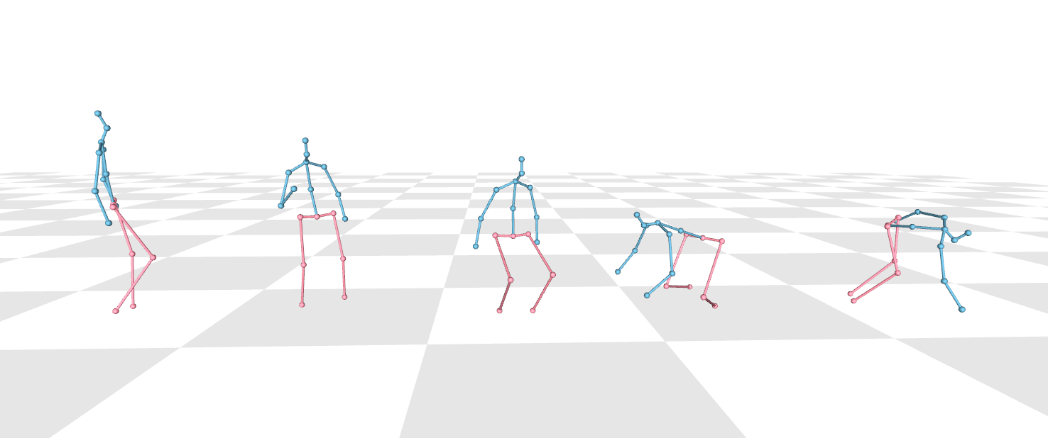
Figure 3: The lower body completed by GFPose given only the upper body. One sample is drawn for each pose.

5.5 Denoise MoCap Data (Noisy 3D $\rightarrow$ Clean 3D)

3D human poses captured from vision-based algorithms or wearable devices often suffer from different types of noises, such as jitters or drifts. Due to the denoising nature of score-based models, it is straightforward to use GFPose to denoise MoCap Data. Following previous works [58], we evaluate the denoising effect of GFPose on a noisy MoCap dataset. Concretely, we add uniform noise and Gaussian noise with different intensities to the test set of H3.6M, and evaluate GFPose on this “noisy H3.6M” dataset. We train GFPose with a masking strategy HPJ-T00 (always activate human level mask with a probability 1.0). At test time, we condition GFPose on $\O$ and replace the initial state $\mathbf{x}(T)$ with the noisy pose. Generally, we choose a smaller start time for smaller noise. Table 7 reports the MPJPE (mm) under Protocol #2 before and after denoising. We find that GFPose can effectively handle different types and intensities of noise. For Gaussian noise with a small variance of 25, GFPose can improve the pose quality by about 24% in terms of MPJPE. For Gaussian noise with a large variance of 400, GFPose can improve the pose quality by about 49%. We also observe consistent improvement in uniform noise. In addition, we report the denoising results on a clean dataset, as shown in the first row of Table 7. A good denoiser should keep minimum adjustment on the clean data. We find our GFPose introduces moderate extra noise on the clean data.

Most previous works [58, 47, 43, 12] learn the pose priors in the SMPL [34] parameter space. While our method learns pose priors on the joint locations. It is hard to directly compare the denoising effect between our method and previous works. Here, we list the denoising performance of a most recent work Pose-NDF[58] as a reference. According to [58], the average intensity of introduced noise is 93.0mm, and the per-vertex error after denoising is 79.6mm. Note that they also leverage additional temporal information to enforce smoothness.

Input Data	MPJPE (before/ after)	Start $T$
GT	0 / 14.7	0.05
GT + $\mathcal{N}(0,25)$	33.1 / 25.0	0.05
GT + $\mathcal{N}(0,100)$	65.5 / 42.8	0.05
GT + $\mathcal{N}(0,400)$	126.0 / 64.6	0.1
GT + $\mathcal{U}(25)$	49.1 / 32.8	0.05
GT + $\mathcal{U}(50)$	96.2 / 50.9	0.1
GT + $\mathcal{U}(100)$	178.2 / 89.4	0.1

Table 7: Denoising results on H3.6M dataset. We report MPJPE (mm) under Protocol #2. $\mathcal{N}$ and $\mathcal{U}$ denote Gaussian and uniform noise respectively. $T$ denotes the start time of RSDE.

5.6 Pose Generation (Noise $\rightarrow$ 3D)

Getting annotated 3D pose is expensive. We show that GFPose can also be used as a pose generator to produce diverse and realistic 3D poses. In this task, we train GFPose with a maksing strategy HPJ-T00. At test time, we condition GFPose on $\O$ to generate random poses from $p_{data}(\mathbf{x})$. To assess the diversity and realism of the generated poses, we train a deterministic pose estimator on the generated data and evaluate it on the test set of H3.6M. Note that the pose estimator gets satisfactory performance only when the generated data are both diverse and realistic. It is in fact a strict metric. We sample 177,200 poses from GFPose to compose the synthetic dataset. While the original H3.6M training set consists of 1,559,752 poses. Table 8 shows that the pose estimator can achieve moderate performance when trained only with the synthetic data. This demonstrates GFPose can draw diverse and realistic samples.

In addition, we find that the generated data can also serve as an augmentation to the existing H3.6M training set and further benefit the training of a deterministic pose estimator. We experiment with different scales of real data and synthetic data to simulate two typical scenarios where MoCap data are scarce or abundant. When the size of Mocap data is small (2,438 samples), increasing the size of synthetic data will continuously improve performance. When the size of Mocap data is large (1,559,752 samples), complementing it with a small proportion of synthetic data can still boost the performance. This further demonstrates the value of GFPose as a pose generator.

Mocap Data (H3.6M)	Synthetic Data (GFPose)	MPJPE
2,438	0	66.1
2,438	1,219	62.0
2,438	2,438	60.0
2,438	177,200	58.1
1,559,752	0	54.3
1,559,752	177,200	53.4
0	177,200	58.1

Table 8: Augment training data with sampled poses from GFPose. We train separate deterministic pose estimators with different combinations of real / synthetic data. The number of 1,559,752 is the size of the H3.6M training set. The number of 2,438 indicates sampling the original H3.6M training set every 640 frames. MPJPE(mm) under Protocol #1 is reported.

5.7 Ablation Study

We ablate different factors that would affect the performance of our model on the 3D pose estimation task, including the number of sampling steps, and the depth and width of the network. As shown in Table 9, more sampling steps or deeper or wider networks do not improve the reconstruction accuracy, but at the expense of greatly reducing the inference speed. We leave the ablation of different condition masking strategies to the Supplementary.

Steps	Blocks	Hidden Dim	MPJPE	FPS
1k	2	1024	35.6	240
0.5k	2	1024	36.1	594
2k	2	1024	35.7	107
1k	3	1024	37.2	154
1k	4	1024	37.1	123
1k	2	512	44.3	461
1k	2	2048	37.6	79
1k	2	4096	37.5	35

Table 9: Ablation Study. We draw 200 samples for each model and report minMPJPE(mm) under Protocol #1. We also compare the inference speed to draw one sample on a NVIDIA 2080Ti GPU.

6 Conclusion and Discussion

We introduce GFPose, a versatile framework to model 3D human pose prior via denoising score matching. GFPose incorporates pose prior and task-specific conditions into gradient fields for various applications. We further propose a condition masking strategy to enhance the versatility. We validate the effectiveness of GFPose on various downstream tasks and demonstrate compelling results.

Limitation Although GFPose has shown great potential in many applications, the reverse sampling process requires repeated model inferences. The overall inference time is proportional to the number of sampling steps, which may limit the use of very large deep networks in real-time scenarios.

Appendix A Details of subVP SDE

In this work, we use the subVP SDE proposed in  [56] to perturb the 3D pose data. Formally,

$$d\mathbf{x}=-\frac{1}{2}\beta(t)\mathbf{x}dt+\sqrt{\beta(t)(1-e^{-2\int_{0}^{t}\beta(s)\,ds})}d\mathbf{w},$$ (7)

where $\mathbf{x}\in\mathbb{R}^{J\times 3}$ denotes the 3D human pose, $\beta(t)$ denotes the noise scale at timestep $t$. The drift coefficient of $\mathbf{x}(t)$ is $\mathbf{f}(\mathbf{x},t)=-\frac{1}{2}\beta(t)\mathbf{x}$. The diffusion coefficient is $g(t)=\sqrt{\beta(t)(1-e^{-2\int_{0}^{t}\beta(s)\,ds})}$. $t\in[0,1]$ is a continuous variable. We adopt the linear scheduled noise scales:

$$\beta(t)=\beta(0)+t\left(\beta(1)-\beta(0)\right).$$ (8)

We empirically set the minimum and maximum noise scale $\beta(0)$ and $\beta(1)$ to $0.1$ and $20.0$, respectively.

Appendix B Closed Form of Loss Function

Because the drift coefficient $\mathbf{f}(\mathbf{x},t)$ is affine, according to [56], the transition kernel $p_{0t}(\mathbf{x}(t)\mid\mathbf{x}(0),\mathbf{c})$ in the loss function (Eq. 6 in the main text) is always a Gaussian distribution, where the mean and variance can be obtained in the closed form:

$$\mathcal{N}\left(\mathbf{x}(t);\mathbf{x}(0)e^{-\frac{1}{2}\int_{0}^{t}\beta(s)\,ds},\left[1-e^{-\int_{0}^{t}\beta(s)\,ds}\right]^{2}\mathbf{I}\right).$$ (9)

Following [52], we choose the weighting function $\lambda(t)=\sigma(t)^{2}$. Thus, the loss function can be written as:

$$\mathcal{L} ={}\mathbb{E}_{\mathcal{U}(t;0,1)}\left[\lambda(t)\left\lVert\mathbf{s}_{\theta}\left(\mathbf{x}(t),t,\mathbf{c}\right)+\frac{\mathbf{x}(t)-\mu}{\sigma^{2}}\right\rVert_{2}^{2}\right]$$ (10)

$$={}\mathbb{E}_{\mathcal{U}(t;0,1)}\left[\left\lVert\sigma(t)\mathbf{s}_{\theta}\left(\mathbf{x}(t),t,\mathbf{c}\right)+\mathbf{z}\right\rVert_{2}^{2}\right],$$

where $\mathbf{z}\sim\mathcal{N}(0,1)$ is random noise. $\mathbf{s}_{\theta}\left(\mathbf{x}(t),t,\mathbf{c}\right)$ is the score network we would like to learn. According to Eq. 9, we can get $\sigma(t)=1-e^{-\int_{0}^{t}\beta(s)\,ds}$.

During training, we uniformly sample the time variable $t$ from $[0,1]$ and sample a noise vector $\mathbf{z}\in\mathbb{R}^{J\times 3}$ from a standard normal distribution. Then we perturb the ground-truth 3D human pose $\mathbf{x}(0)$ according to Eq. 9 to get the noisy 3D pose $\mathbf{x}(t)$:

$$\mathbf{x}(t)=\mathbf{x}(0)e^{-\frac{1}{2}\int_{0}^{t}\beta(s)\,ds}+\mathbf{z}\cdot\left(1-e^{-\int_{0}^{t}\beta(s)\,ds}\right).$$ (11)

Then we can compute the loss according to Eq. 10 to train the score network.

Appendix C Network Architecture

Fig. 4 shows the architecture of our score network $\mathbf{s}_{\theta}$. It is a simple fully-connected network with a structure similar to [37]. Following [37], we set the hidden dimension of all FC layers to $1024$. We adopt group normalization [65] with the number of groups set to $32$. We use SiLU [17] as nonlinear activation and set the dropout rate to $0.25$.

Appendix D Pose Sampling

To sample human poses from the learned pose prior $p_{data}(\mathbf{x}|\mathbf{c})$, we need to solve the reverse-time SDE (Eq. 5 in the main text). Following [56], we simulate the RSDE via the Predictor-Corrector (PC) sampler. We use the Euler-Maruyama solver as the predictor and Identity as the corrector. We set the number of sampling steps $N=1000$, start time $T=1.0$ and the end time $eps=1e-3$. Please refer to Alg. 1 for the detailed sampling process.

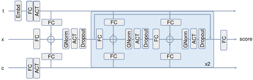
Figure 4: Architecture of the score network $\mathbf{s}_{\theta}$. It is a plain fully connected network consisting of 2 residual blocks. $\mathbf{x}\in\mathbb{R}^{J\times 3}$ denotes noisy 3D poses. $\mathbf{c}$ denotes different task conditions, e.g.detected 2D poses. $t$ denotes the timestep. $\oplus$ denotes the sum operator.

Appendix E Detailed Settings for Different Tasks

In this section, we detail how we train and use our model for each task described in the main text. The difference lies in the types of conditions, masking strategy and sampling process.

Monocular 3D Human Pose Estimation

During training, GFPose conditions on the detected 2D pose without any condition masking strategy, i.e., HPJ-000. At inference, we sample a noise vector $\mathbf{x}(T)\in\mathbb{R}^{J\times 3}$ from a standard normal distribution $\mathcal{N}(0,1)$, and gradually adjust it according to the standard sampling process described in Alg. 1.

Algorithm 1 Sampling from $p_{data}(\mathbf{x}|\mathbf{c})$

1:learned $\mathbf{s}_{\theta}$; sampling step $N$; condition $c$; start time $T$; end time $eps$

2:$\mathbf{f}(\mathbf{x},t)\leftarrow-\frac{1}{2}\beta(t)\mathbf{x}$

3:$g(t)\leftarrow\sqrt{\beta(t)(1-e^{-2\int_{0}^{t}\beta(s)\,ds})}$

4:$dt\leftarrow\frac{1}{N}$

5:$\mathbf{x}_{N}\sim\mathcal{N}(0,1)$

6:for $i\leftarrow N-1$ to $0$ do

7:     $t\leftarrow eps+(T-eps)\cdot\frac{i+1}{N}$

8:     $\mathbf{x}_{i}^{\prime}\leftarrow\mathbf{x}_{i+1}-\left[\mathbf{f}(\mathbf{x}_{i+1},t)-g(t)^{2}\mathbf{s}_{\theta}\left(\mathbf{x}_{i+1},t,\mathbf{c}\right)\right]dt$

9:     $\mathbf{z}\sim\mathcal{N}(0,1)$

10:     $\mathbf{x}_{i}\leftarrow\mathbf{x}_{i}^{\prime}+g(t)\sqrt{dt}\mathbf{z}$

11:end for

12:return $\mathbf{x}_{0}$

Pose Completion (2D $\rightarrow$ 3D)

During training, GFPose conditions on the detected 2D pose with masking strategy HPJ-001 and HPJ-020 for missing joint and part completion, respectively. Here, we explore three sampling approaches. The first is the standard conditional inference process as described in Alg. 1. The second is the imputation approach proposed in [56]. We also try combining these two inference techniques as the third approach. In this task, we adopt the combination approach as it performs best. In Sec. G, we will further compare different inference approaches.

Pose Completion (3D $\rightarrow$ 3D)

During training, GFPose conditions on the gt 3D pose with a masking strategy HPJ-020 for missing body part completion. We also adopt the combination approach during sampling.

Denoising Mocap Data

In this task, GFPose is trained with a masking strategy HPJ-T00, i.e., human level mask is always activated and the condition is always zero. To use this model for denoising, we condition the model on $\O$ and start the sampling process from a noisy 3D pose $\mathbf{x}(T)\in\mathbb{R}^{J\times 3}$ instead of a noise vector. We set the start time $T$ of reverse-time SDE to a small value of $0.05$ or $0.1$ instead of the default value $1.0$, as shown in Table 7 in the main text. Intuitively, a smaller start time notifies the score network $\mathbf{s}_{\theta}$ that we are not starting from pure noise, so a small adjustment is sufficient.

Pose Generation

For generation, GFPose is trained with a masking strategy HPJ-T00. During inference, GFPose conditions on $\O$ and gradually adjusts the noise vector $\mathbf{x}(T)\in\mathbb{R}^{J\times 3}$ sampled from a standard normal distribution $\mathcal{N}(0,1)$ to generate realistic and diverse 3D poses.

Appendix F Train A Unified Model for Various Tasks

Instead of training separate models for different tasks, we can also train one unified model for all tasks. Concretely, we active all three levels of masks during training. There are two different choices to train such a unified model. 1) We only condition on the detected 2D pose, i.e. $\mathbf{c}\subset\{\mathbf{x}_{2d}\}$. We call this model “U2D”. 2) We condition on the detected 2D pose $0.9$ and the 3D pose with a probability of $0.1$, i.e. $\mathbf{c}\subset\{\mathbf{x}_{2d},\mathbf{x}_{3d}\}$. We call this model “U3D”. Note that the 3D condition shares the same masking strategy as the 2D condition. This helps the model to explicitly establish the relationship between different 3D body parts. We quantitatively study the unified model in the following.

$p_{h}$	$p_{p}$	$p_{j}$	2D	3D	minMPJPE ($S=1/200$)
0.0	0.0	0.0	✓	✗	51.0 / 35.6
0.1	0.0	0.0	✓	✗	50.8 /35.8
0.0	0.1	0.0	✓	✗	50.5 / 35.1
0.0	0.0	0.1	✓	✗	51.7 / 36.4
0.1	0.1	0.0	✓	✗	51.0 / 36.0
0.0	0.1	0.1	✓	✗	51.1 / 35.5
0.1	0.1	0.1	✓	✗	52.3 / 36.7
0.1	0.2	0.1	✓	✗	52.4 / 36.5
0.1	0.1	0.1	✓	✓	51.3 / 35.9
0.1	0.2	0.1	✓	✓	51.6 / 36.4

Table 10: Effects of condition masking strategies on monocular 3D human pose estimation. We report minMPJPE(mm) on H3.6M dataset under protocol #1. S denotes the number of samples. $p_{h}$, $p_{p}$ and $p_{j}$ respectively denote the probability of activating human-, part- and joint- level masks.

Monocular 3D Pose Estimation

We first ablate condition masking strategies on monocular 3D human pose estimation. Table 10 reports the minMPJPE(mm) for different models on H3.6M dataset. We can find that training with human- or part- level masks slightly boosts the performance of pose estimation ($\sim$0.5mm). Training with the mixed masking strategy, i.e. the unified model “U2D” (3rd and 4th row from last) causes a slight drop ($\sim$1mm) in reconstruction accuracy. Further incorporating 3D pose (1st and 2nd row from last, “U3D”) can benefit the pose estimation task.

Pose Completion

We compare the two unified models “U2D” and “U3D” on the pose completion task. From Table 11, we can observe that the unified models perform slightly worse than the specifically trained model when recovering occluded body parts. However, they achieve competitive results as the specifically trained model when recovering occluded random joints and significantly outperforms the SOTA [28]. From Table 12, we can find that the unified model “U3D” performs quite well when recovering from partial 3D observations. Note that “U2D” cannot directly apply to this task unless through the imputation technique introduced in the next section.

Pose Denoising

Table 13 shows that the unified model performs slightly better on small noise intensities while the specifically trained model (HPJ-T00) performs slightly better on large noise intensities.

Pose Generation

We train 3 deterministic pose estimators on the synthetic poses generated by HPJ-T00, “U2D” and “U3D”, respectively. Table 14 shows that the specifically trained model HPJ-T00 can generate the best quality poses. Unified models also show competitive results.

Summary

We can trade very little performance loss for a versatile unified model “U3D”.

Occ. Parts	Sep.	U2D	U3D	Li et al.  [28]
1 Joint	37.8	37.5	37.6	58.8
2 Joints	39.6	39.8	39.5	64.6
2 Legs	53.5	54.9	53.8	-
2 Arms	60.0	62.1	60.4	-
Left Leg + Left arm	54.6	56.4	55.2	-
Right leg + Right arm	53.1	54.3	53.5	-

Table 11: Recover 3D pose from partial 2D observation. We compare the unified models (“U2D” and “U3D”) and the model specifically trained for this task (Sep. here means HPJ-001 and HPJ-020, reported in the main text. Please refer to Section E). We report minMPJPE(mm) on H3.6M dataset under protocol #1. 200 samples are drawn.

Occ. Parts	Sep.	U3D
Right Leg	5.2	5.6
Left Leg	5.8	5.9
Left Arm	9.4	9.7
Right Arm	8.9	9.0

Table 12: Recover 3D pose from partial 3D observation. We compare the unified models (“U2D” and “U3D”) and the model specifically trained for this task (Sep., reported in the main text. Please refer to Section E for details) on H3.6M dataset and report minMPJPE(mm) under protocol #1. 200 samples are drawn.

Noisy Data	Base	Sep.	U2D	U3D	Start $T$
GT	0	14.7	13.8	14.0	0.05
GT + $\mathcal{N}(0,25)$	33.1	25.0	25.1	24.8	0.05
GT + $\mathcal{N}(0,100)$	65.5	42.8	44.0	43.5	0.05
GT + $\mathcal{N}(0,400)$	126.0	64.6	65.5	65.2	0.1
GT + $\mathcal{U}(25)$	49.1	32.8	33.5	33.0	0.05
GT + $\mathcal{U}(50)$	96.2	50.9	51.0	51.0	0.1
GT + $\mathcal{U}(100)$	178.2	89.4	91.4	91.1	0.1

Table 13: Denoising results on H3.6M dataset. We report MPJPE (mm) under Protocol #2. “Sep.” here indicates model “HPJ-T00”. (Please refer to Section E) “Base” represents the MPJPE(mm) of noisy data. $\mathcal{N}$ and $\mathcal{U}$ denote Gaussian and uniform noise, respectively. $T$ denotes the start time of RSDE.

Model	Sep.	U2D	U3D
MPJPE	58.1	60.8	59.7

Table 14: Quality comparison of generated poses. We train 3 deterministic pose estimators on the poses generated by 3 different GFPose models (Sep. here means “HPJ-T00”. Please refer to Section E). Then we evaluate them on the H3.6M test set. MPJPE(mm) under Protocol #1 is reported.

Appendix G Different Sampling Approaches

Imputation [56] provides a flexible way to use score models for imputation tasks, like image inpainting and colorization. By repeatedly replacing part of the data in $\mathbf{x}(t)$ with the observed data $\mathbf{x}_{obs}$ during the sampling process, imputation allows us to use unconditional score models to impute the missing dimensions of data. Here, we can also view the 3D pose estimation and the completion task as imputation tasks, i.e., we impute the depth of 2D poses or impute the missing body joints. We compare the performance of imputation, conditional inference and the combination of these 2 techniques in Table 15, 17, 16. We can get the following observations: (1) conditional inference generally performs better than imputation. (2) Combining two inference approaches can yield consistently better results than either approach alone on pose completion tasks. (3) Conditional inference performs best on the 3D human pose estimation task. (4) Imputation works better with unconditional models (HPJ-T00).

Appendix H More Qualitative Results

We show more qualitative results for multi-hypothesis 3D pose estimation (Figure 5), pose completion (Figure 6), pose denoising and generation (Figure 7). All poses are sampled from the unified model “U3D”.

Model	Cond.	Impt.	Cond.+Impt.
HPJ-010	35.1	49.5	36.8
HPJ-T00	-	42.3	-
U2D	36.7	43.0	37.2
U3D	35.9	43.0	37.1

Table 15: Comparison between different sampling approaches on 3D pose estimation. HPJ-T00 means we always activate the human level mask and learn an unconditional score model.

Model	Cond.	Impt.	Cond.+Impt.
HPJ-020	53.9	72.8	53.5
HPJ-T00	-	64.9	-
U2D	55.8	67.4	54.9
U3D	54.6	66.8	53.8

Table 16: Comparison between different sampling approaches on pose completion from partial 2D observation (2 legs). HPJ-T00 indicates an unconditional score model.

Model	Cond.	Impt.	Cond.+Impt.
HPJ-020	5.3	8.3	5.2
HPJ-T00	-	6.0	-
U2D	-	6.2	-
U3D	8.6	6.1	5.6

Table 17: Comparison between different sampling approaches on pose completion from partial 3D observation (rigth leg). HPJ-T00 indicates an unconditional score model.

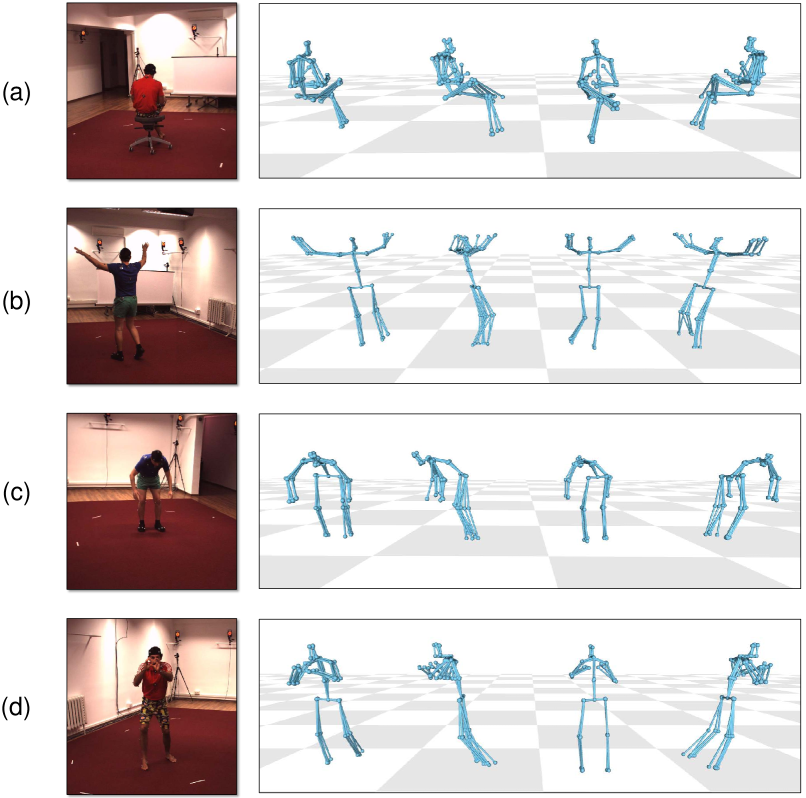
Figure 5: Multi-hypothesis 3D human pose estimation. We randomly sample $5$ hypotheses from GFPose and show them from $4$ different viewpoints. From left to right, the plausible poses are rotated 90 degrees clockwise around the z-axis.

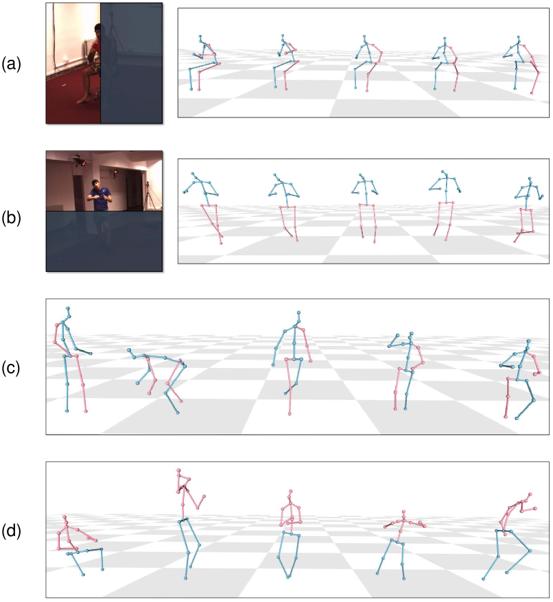
Figure 6: Pose completion. GFPose can recover full 3D human body from partial observations. 3D poses corresponding to the visible observation and missing observation are plotted in different colors for clarity. (a)(b) Recover full 3D human body from partial 2D image. We show five plausible poses sampled from GFPose. (a) Left side of the body is invisible. (b) Lower body is invisible. (c)(d) Recover full 3D human body from partial 3D poses. For each instance, we sample and plot one plausible completion. (c) Left arm and right leg are missing. They are completed by GFPose. (d) Upper body are missing and completed by GFPose.

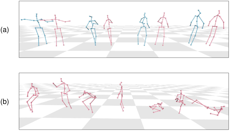
Figure 7: Pose denoising and generation. (a) Pose denoising. We add Gaussian noise $\sim\mathcal{N}(0,100)$ onto GT and denoise it with GFPose. Nosiy poses and denoised poses are plotted in different colors. GFPose can effectively correct unreasonable poses. (b) Pose generation. GFPose can generate diverse and realistic poses.

References

- [1] Karan Ahuja, Chris Harrison, Mayank Goel, and Robert Xiao. Mecap: Whole-body digitization for low-cost vr/ar headsets. In Proceedings of the 32nd Annual ACM Symposium on User Interface Software and Technology, pages 453–462, 2019.
- [2] Ijaz Akhter and Michael J Black. Pose-conditioned joint angle limits for 3d human pose reconstruction. In Proceedings of the IEEE conference on computer vision and pattern recognition, pages 1446–1455, 2015.
- [3] Brian DO Anderson. Reverse-time diffusion equation models. Stochastic Processes and their Applications, 12(3):313–326, 1982.
- [4] Mykhaylo Andriluka, Leonid Pishchulin, Peter Gehler, and Bernt Schiele. 2d human pose estimation: New benchmark and state of the art analysis. In Proceedings of the IEEE Conference on computer Vision and Pattern Recognition, pages 3686–3693, 2014.
- [5] Federica Bogo, Angjoo Kanazawa, Christoph Lassner, Peter Gehler, Javier Romero, and Michael J Black. Keep it smpl: Automatic estimation of 3d human pose and shape from a single image. In European conference on computer vision, pages 561–578. Springer, 2016.
- [6] Ruojin Cai, Guandao Yang, Hadar Averbuch-Elor, Zekun Hao, Serge Belongie, Noah Snavely, and Bharath Hariharan. Learning gradient fields for shape generation. In European Conference on Computer Vision, pages 364–381. Springer, 2020.
- [7] Yilun Chen, Zhicheng Wang, Yuxiang Peng, Zhiqiang Zhang, Gang Yu, and Jian Sun. Cascaded pyramid network for multi-person pose estimation. In Proceedings of the IEEE conference on computer vision and pattern recognition, pages 7103–7112, 2018.
- [8] Yu Cheng, Bo Yang, Bo Wang, Wending Yan, and Robby T Tan. Occlusion-aware networks for 3d human pose estimation in video. In Proceedings of the IEEE/CVF international conference on computer vision, pages 723–732, 2019.
- [9] Yalin Cheng, Pengfei Yi, Rui Liu, Jing Dong, Dongsheng Zhou, and Qiang Zhang. Human-robot interaction method combining human pose estimation and motion intention recognition. In 2021 IEEE 24th International Conference on Computer Supported Cooperative Work in Design (CSCWD), pages 958–963. IEEE, 2021.
- [10] Hai Ci, Xiaoxuan Ma, Chunyu Wang, and Yizhou Wang. Locally connected network for monocular 3d human pose estimation. IEEE TPAMI, pages 1–1, 2020.
- [11] Hai Ci, Chunyu Wang, Xiaoxuan Ma, and Yizhou Wang. Optimizing network structure for 3d human pose estimation. In Proceedings of the IEEE/CVF international conference on computer vision, pages 2262–2271, 2019.
- [12] Andrey Davydov, Anastasia Remizova, Victor Constantin, Sina Honari, Mathieu Salzmann, and Pascal Fua. Adversarial parametric pose prior. In Proceedings of the IEEE/CVF Conference on Computer Vision and Pattern Recognition, pages 10997–11005, 2022.
- [13] Junting Dong, Qing Shuai, Yuanqing Zhang, Xian Liu, Xiaowei Zhou, and Hujun Bao. Motion capture from internet videos. In ECCV, 2020.
- [14] Haodong Duan, Yue Zhao, Kai Chen, Dian Shao, Dahua Lin, and Bo Dai. Revisiting skeleton-based action recognition. In CVPR, 2022.
- [15] Qing Gao, Jinguo Liu, Zhaojie Ju, and Xin Zhang. Dual-hand detection for human–robot interaction by a parallel network based on hand detection and body pose estimation. IEEE Transactions on Industrial Electronics, 66(12):9663–9672, 2019.
- [16] H Hatze. A three-dimensional multivariate model of passive human joint torques and articular boundaries. Clinical Biomechanics, 12(2):128–135, 1997.
- [17] Dan Hendrycks and Kevin Gimpel. Gaussian error linear units (gelus). arXiv preprint arXiv:1606.08415, 2016.
- [18] Aapo Hyvärinen and Peter Dayan. Estimation of non-normalized statistical models by score matching. Journal of Machine Learning Research, 6(4), 2005.
- [19] Catalin Ionescu, Dragos Papava, Vlad Olaru, and Cristian Sminchisescu. Human3.6m: Large scale datasets and predictive methods for 3d human sensing in natural environments. IEEE TPAMI, 2014.
- [20] Ehsan Jahangiri and Alan L Yuille. Generating multiple diverse hypotheses for human 3d pose consistent with 2d joint detections. In Proceedings of the IEEE International Conference on Computer Vision Workshops, pages 805–814, 2017.
- [21] Michael Janner, Yilun Du, Joshua B Tenenbaum, and Sergey Levine. Planning with diffusion for flexible behavior synthesis. arXiv preprint arXiv:2205.09991, 2022.
- [22] Jiaxi Jiang, Paul Streli, Huajian Qiu, Andreas Fender, Larissa Laich, Patrick Snape, and Christian Holz. Avatarposer: Articulated full-body pose tracking from sparse motion sensing. In Proceedings of European Conference on Computer Vision. Springer, 2022.
- [23] Angjoo Kanazawa, Michael J. Black, David W. Jacobs, and Jitendra Malik. End-to-end recovery of human shape and pose. In Computer Vision and Pattern Regognition (CVPR), 2018.
- [24] Diederik P Kingma and Jimmy Ba. Adam: A method for stochastic optimization. arXiv preprint arXiv:1412.6980, 2014.
- [25] Muhammed Kocabas, Nikos Athanasiou, and Michael J. Black. Vibe: Video inference for human body pose and shape estimation. In The IEEE Conference on Computer Vision and Pattern Recognition (CVPR), June 2020.
- [26] Timotej Kodek and Marko Munih. Identifying shoulder and elbow passive moments and muscle contributions during static flexion-extension movements in the sagittal plane. In IEEE/RSJ International Conference on Intelligent Robots and Systems, volume 2, pages 1391–1396. IEEE, 2002.
- [27] Nikos Kolotouros, Georgios Pavlakos, Dinesh Jayaraman, and Kostas Daniilidis. Probabilistic modeling for human mesh recovery. In ICCV, 2021.
- [28] Chen Li and Gim Hee Lee. Generating multiple hypotheses for 3d human pose estimation with mixture density network. In The IEEE Conference on Computer Vision and Pattern Recognition (CVPR), June 2019.
- [29] Chen Li and Gim Hee Lee. Weakly supervised generative network for multiple 3d human pose hypotheses. arXiv preprint arXiv:2008.05770, 2020.
- [30] Wenhao Li, Hong Liu, Hao Tang, Pichao Wang, and Luc Van Gool. Mhformer: Multi-hypothesis transformer for 3d human pose estimation. In Proceedings of the IEEE/CVF Conference on Computer Vision and Pattern Recognition, pages 13147–13156, 2022.
- [31] Huei-Yung Lin and Ting-Wen Chen. Augmented reality with human body interaction based on monocular 3d pose estimation. In International Conference on Advanced Concepts for Intelligent Vision Systems, pages 321–331. Springer, 2010.
- [32] Hung Yu Ling, Fabio Zinno, George Cheng, and Michiel Van De Panne. Character controllers using motion vaes. ACM Transactions on Graphics (TOG), 39(4):40–1, 2020.
- [33] Hongyi Liu and Lihui Wang. Collision-free human-robot collaboration based on context awareness. Robotics and Computer-Integrated Manufacturing, 67:101997, 2021.
- [34] Matthew Loper, Naureen Mahmood, Javier Romero, Gerard Pons-Moll, and Michael J Black. Smpl: A skinned multi-person linear model. ACM transactions on graphics (TOG), 34(6):1–16, 2015.
- [35] Shitong Luo and Wei Hu. Score-based point cloud denoising. In Proceedings of the IEEE/CVF International Conference on Computer Vision, pages 4583–4592, 2021.
- [36] Xiaoxuan Ma, Jiajun Su, Chunyu Wang, Hai Ci, and Yizhou Wang. Context modeling in 3d human pose estimation: A unified perspective. In CVPR, 2021.
- [37] Julieta Martinez, Rayat Hossain, Javier Romero, and James J Little. A simple yet effective baseline for 3d human pose estimation. In ICCV, pages 2640–2649, 2017.
- [38] Dushyant Mehta, Helge Rhodin, Dan Casas, Pascal Fua, Oleksandr Sotnychenko, Weipeng Xu, and Christian Theobalt. Monocular 3d human pose estimation in the wild using improved cnn supervision. In 3D Vision (3DV), 2017 Fifth International Conference on, 2017.
- [39] Dushyant Mehta, Srinath Sridhar, Oleksandr Sotnychenko, Helge Rhodin, Mohammad Shafiei, Hans-Peter Seidel, Weipeng Xu, Dan Casas, and Christian Theobalt. Vnect: Real-time 3d human pose estimation with a single rgb camera. Acm transactions on graphics (tog), 36(4):1–14, 2017.
- [40] Erik Murphy-Chutorian and Mohan Manubhai Trivedi. Head pose estimation and augmented reality tracking: An integrated system and evaluation for monitoring driver awareness. IEEE Transactions on intelligent transportation systems, 11(2):300–311, 2010.
- [41] Alejandro Newell, Kaiyu Yang, and Jia Deng. Stacked hourglass networks for human pose estimation. In European conference on computer vision, pages 483–499. Springer, 2016.
- [42] Tuomas Oikarinen, Daniel Hannah, and Sohrob Kazerounian. Graphmdn: Leveraging graph structure and deep learning to solve inverse problems. In 2021 International Joint Conference on Neural Networks (IJCNN), pages 1–9. IEEE, 2021.
- [43] Georgios Pavlakos, Vasileios Choutas, Nima Ghorbani, Timo Bolkart, Ahmed AA Osman, Dimitrios Tzionas, and Michael J Black. Expressive body capture: 3d hands, face, and body from a single image. In Proceedings of the IEEE/CVF conference on computer vision and pattern recognition, pages 10975–10985, 2019.
- [44] Dario Pavllo, Christoph Feichtenhofer, David Grangier, and Michael Auli. 3d human pose estimation in video with temporal convolutions and semi-supervised training. In Proceedings of the IEEE/CVF Conference on Computer Vision and Pattern Recognition, pages 7753–7762, 2019.
- [45] Mathis Petrovich, Michael J. Black, and Gül Varol. Action-conditioned 3D human motion synthesis with transformer VAE. In International Conference on Computer Vision (ICCV), pages 10985–10995, October 2021.
- [46] Paweł A Pierzchlewicz, R James Cotton, Mohammad Bashiri, and Fabian H Sinz. Multi-hypothesis 3d human pose estimation metrics favor miscalibrated distributions. arXiv preprint arXiv:2210.11179, 2022.
- [47] Davis Rempe, Tolga Birdal, Aaron Hertzmann, Jimei Yang, Srinath Sridhar, and Leonidas J Guibas. Humor: 3d human motion model for robust pose estimation. In Proceedings of the IEEE/CVF International Conference on Computer Vision, pages 11488–11499, 2021.
- [48] Ruizhi Shao, Zerong Zheng, Hongwen Zhang, Jingxiang Sun, and Yebin Liu. Diffustereo: High quality human reconstruction via diffusion-based stereo using sparse cameras. arXiv preprint arXiv:2207.08000, 2022.
- [49] Saurabh Sharma, Pavan Teja Varigonda, Prashast Bindal, Abhishek Sharma, and Arjun Jain. Monocular 3d human pose estimation by generation and ordinal ranking. In The IEEE International Conference on Computer Vision (ICCV), October 2019.
- [50] Chence Shi, Shitong Luo, Minkai Xu, and Jian Tang. Learning gradient fields for molecular conformation generation. In International Conference on Machine Learning, pages 9558–9568. PMLR, 2021.
- [51] Yang Song, Conor Durkan, Iain Murray, and Stefano Ermon. Maximum likelihood training of score-based diffusion models. Advances in Neural Information Processing Systems, 34:1415–1428, 2021.
- [52] Yang Song and Stefano Ermon. Generative modeling by estimating gradients of the data distribution. Advances in Neural Information Processing Systems, 32, 2019.
- [53] Yang Song and Stefano Ermon. Improved techniques for training score-based generative models. Advances in neural information processing systems, 33:12438–12448, 2020.
- [54] Yang Song, Sahaj Garg, Jiaxin Shi, and Stefano Ermon. Sliced score matching: A scalable approach to density and score estimation. In Uncertainty in Artificial Intelligence, pages 574–584. PMLR, 2020.
- [55] Yang Song, Liyue Shen, Lei Xing, and Stefano Ermon. Solving inverse problems in medical imaging with score-based generative models. arXiv preprint arXiv:2111.08005, 2021.
- [56] Yang Song, Jascha Sohl-Dickstein, Diederik P Kingma, Abhishek Kumar, Stefano Ermon, and Ben Poole. Score-based generative modeling through stochastic differential equations. arXiv preprint arXiv:2011.13456, 2020.
- [57] Mohammed Suhail, Abhay Mittal, Behjat Siddiquie, Chris Broaddus, Jayan Eledath, Gerard Medioni, and Leonid Sigal. Energy-based learning for scene graph generation. In Proceedings of the IEEE/CVF Conference on Computer Vision and Pattern Recognition, pages 13936–13945, 2021.
- [58] Garvita Tiwari, Dimitrije Antić, Jan Eric Lenssen, Nikolaos Sarafianos, Tony Tung, and Gerard Pons-Moll. Pose-ndf: Modeling human pose manifolds with neural distance fields. In European Conference on Computer Vision, pages 572–589. Springer, 2022.
- [59] Pascal Vincent. A connection between score matching and denoising autoencoders. Neural computation, 23(7):1661–1674, 2011.
- [60] Tom Wehrbein, Marco Rudolph, Bodo Rosenhahn, and Bastian Wandt. Probabilistic monocular 3d human pose estimation with normalizing flows. In Proceedings of the IEEE/CVF international conference on computer vision, pages 11199–11208, 2021.
- [61] Tom Wehrbein, Marco Rudolph, Bodo Rosenhahn, and Bastian Wandt. Probabilistic monocular 3d human pose estimation with normalizing flows. In ICCV, 2021.
- [62] Max Welling and Yee W Teh. Bayesian learning via stochastic gradient langevin dynamics. In Proceedings of the 28th international conference on machine learning (ICML-11), pages 681–688, 2011.
- [63] Alexander Winkler, Jungdam Won, and Yuting Ye. Questsim: Human motion tracking from sparse sensors with simulated avatars. arXiv preprint arXiv:2209.09391, 2022.
- [64] Mingdong Wu, Fangwei Zhong, Yulong Xia, and Hao Dong. Targf: Learning target gradient field for object rearrangement. arXiv preprint arXiv:2209.00853, 2022.
- [65] Yuxin Wu and Kaiming He. Group normalization. In Proceedings of the European conference on computer vision (ECCV), pages 3–19, 2018.
- [66] Tianhan Xu and Wataru Takano. Graph stacked hourglass networks for 3d human pose estimation. In CVPR, 2021.
- [67] Jackie Yang, Tuochao Chen, Fang Qin, Monica S Lam, and James A Landay. Hybridtrak: Adding full-body tracking to vr using an off-the-shelf webcam. In CHI Conference on Human Factors in Computing Systems, pages 1–13, 2022.
- [68] Ailing Zeng, Xiao Sun, Fuyang Huang, Minhao Liu, Qiang Xu, and Stephen Lin. Srnet: Improving generalization in 3d human pose estimation with a split-and-recombine approach. In European Conference on Computer Vision, pages 507–523. Springer, 2020.
- [69] Ailing Zeng, Xiao Sun, Lei Yang, Nanxuan Zhao, Minhao Liu, and Qiang Xu. Learning skeletal graph neural networks for hard 3d pose estimation. In Proceedings of the IEEE/CVF International Conference on Computer Vision, pages 11436–11445, 2021.
- [70] Zhe Zhang, Chunyu Wang, Wenhu Qin, and Wenjun Zeng. Fusing wearable imus with multi-view images for human pose estimation: A geometric approach. In Proceedings of the IEEE/CVF Conference on Computer Vision and Pattern Recognition, pages 2200–2209, 2020.
- [71] Long Zhao, Xi Peng, Yu Tian, Mubbasir Kapadia, and Dimitris N. Metaxas. Semantic graph convolutional networks for 3d human pose regression. In IEEE Conference on Computer Vision and Pattern Recognition (CVPR), pages 3425–3435, 2019.
- [72] Ce Zheng, Sijie Zhu, Matias Mendieta, Taojiannan Yang, Chen Chen, and Zhengming Ding. 3d human pose estimation with spatial and temporal transformers. In Proceedings of the IEEE/CVF International Conference on Computer Vision, pages 11656–11665, 2021.