Score function-based tests for ultrahigh-dimensional linear models

Abstract

To sufficiently exploit the model structure under the null hypothesis such that the conditions on the whole model can be mild, this paper investigates score function-based tests to check the significance of an ultrahigh-dimensional sub-vector of the model coefficients when the nuisance parameter vector is also ultrahigh-dimensional in linear models. We first reanalyze and extend a recently proposed score function-based test to derive, under weaker conditions, its limiting distributions under the null and local alternative hypotheses. As it may fail to work when the correlation between testing covariates and nuisance covariates is high, we propose an orthogonalized score function-based test with two merits: debiasing to make the non-degenerate error term degenerate and reducing the asymptotic variance to enhance the power performance. Simulations evaluate the finite-sample performances of the proposed tests, and a real data analysis illustrates its application.

Keywords: Ultrahigh-dimensional inference; U-statistics; Orthogonalization.

1 Introduction

It is important to check whether the covariates of interest contribute to the response, given the other covariates. In linear regression models, this is formulated as testing whether the parametric vector of interest is equal to zero. This paper studies inference of ultrahigh-dimensional parameter vector of interest with ultrahigh-dimensional nuisance parameter vector. This problem is of great importance in practice. For instance, researchers may aim to test whether a gene pathway, consisting of ultrahigh-dimensional genes for the same biological functions, is important for certain clinical outcome, given the other ultrahigh-dimensional genes.

For this challenging problem, there are several proposals available in the literature. The coordinate-based maximum tests have been proposed recently. See for instance Ning and Liu, (2017), Zhang and Cheng, (2017), Dezeure et al., (2017), Ma et al., (2021) and Wu et al., (2021). These methods are computationally expensive because many penalized optimization implementations with ultrahigh-dimensional parameter vector are involved. Further, these tests require the sparsity assumption on both nuisance parameter vector and parameter vector of interest, otherwise, the max-type statistics would have relatively low power. A Wald-type test was suggested by Guo et al., (2021), which is computationally low costed. They imposed the boundedness of eigenvalues of covariance matrix and sparse structure on the whole parameter vector. To tackle the problem in the study of the asymptotic properties, brought by too small variance (Guo et al., (2021) pointed out), a positive tuning parameter over the sample size is added to the estimated variance. As the limiting null distribution remains untractable, the critical values determined by their method cause the test conservative in theory (see the discussion on page 11 of Guo et al., (2021)). But in practice, the test could be either very liberal or very conservative in different models as numerical studies in Section 6 of our paper indicate.

Score function-based testing procedures are also popular. As this method can easily exploit the information contained in the null hypothesis, mild conditions on the whole model are in need. This is particularly useful in ultrahigh dimensional paradigms. When the dimension of the nuisance parameter vector is low or diverging at relatively slow rate, and the parameter vector of interest is high-dimensional, the references include Goeman et al., (2006), Zhong and Chen, (2011), Guo and Chen, (2016) (for generalized linear models), Cui et al., (2018), and Guo et al., (2022). The recent development of score function-based testing procedure is made by Chen et al., (2022) who extended the score function-based test of Guo and Chen, (2016) to handle ultra-high dimensional nuisance parameter vector. Due to the adoption of score function, only the nuisance parameter vector requires the sparsity assumption, and the dimension of the parameter vector of interest can grow polynomially with the sample size to guarantee nontrivial power. As a result, this test is suitable under dense alternative hypotheses. Chen et al., (2022) showed some merits of their test in numerical studies. In theory, the eigenvalue boundedness assumption on covariance matrix is still imposed to control the correlations between covariates and the asymptotic limiting distributions under the local alternatives are not established. Although the limiting null distribution was established (Theorem 1, Chen et al., (2022)), some technical details need further careful checks.

The above observations motivate us to further study the score function-based test for linear models, extend the results in the literature and propose new test to handle high correlation between nuisance and testing covariates. To be specific, we will do the following. First, we need to reanalyze, under weaker conditions, the properties of the test statistic and extend the results to the case where the testing parameter and nuisance parameter vectors are ultrahigh dimensional simultaneously at the rates up to the exponential of the sample size. To this end, we derive the limiting distributions under the null and local alternative hypotheses. Second, when the correlation between the covariates of interest and the nuisance covariates is strong, a non-negligible bias causes that the tests in Chen et al., (2022) fail to work. Therefore, we propose an orthogonalization procedure to reduce the possible bias. Although this technique has been adopted in the recent high-dimensional inference literature (Zhang and Zhang,, 2014; Van de Geer et al.,, 2014; Javanmard and Montanari,, 2014; Belloni et al.,, 2015; Chernozhukov et al.,, 2018), to the best of our knowledge, it has not been applied to constructing test statistics based on the quadratic norm of the score function for ultra-high dimensional testing parameter vector. Two merits shown in our investigation are as follows. The orthogonalization can debiase the error terms and convert the non-degenerate error terms to degenerate, thus relaxing the correlation assumption between the covariates of interest and nuisance covariates; it can also reduce the variance of the test statistic and thus enhance the power performance, which was not observed in the literature.

Technically, we establish the asymptotic normality of the two proposed test statistics in a different way from those used by Zhong and Chen, (2011); Guo and Chen, (2016); Cui et al., (2018) for the quadratic norm-based test statistics. Instead of calculating the relatively complex spectral norm of the high dimensional sample matrix, we derive the order of element-max norm of the high-dimensional $U$-statistics with the help of maximal inequalities established in Chernozhukov et al., (2015) and Chen, (2018). The technique developed in this paper can be useful for other high-dimensional inference problems.

The rest of the paper is organized as follows. Section 2 re-analyzes the test statistic in Chen et al., (2022) to handle the case with higher dimensional parameter vector of interest and presents the limiting distributions under both null and local alternative hypotheses. The failure of this test statistic in the high correlation case is also discussed. Section 3 introduces the orthogonalization procedure. Section 4 contains an oracle inference procedure to illustrate the merits of the orthogonalization approach. Further, Section 5 develops an orthogonalization-based test in the general case and derives the relevant asymptotic analysis. Section 6 presents simulation studies and a real data analysis. Section 7 offers some conclusions. The detailed proofs of the theoretical properties are in the Appendix. The Supplementary Materials include some proofs of the theoretical properties, technical lemmas, and additional simulation results.

Before closing this section, we introduce some necessary notations. For a $d$-dimension vector $\mathbf{U}$, write $\lVert\mathbf{U}\rVert_{r}=(\sum_{k=1}^{d}|U_{k}|^{r})^{1/r}$ and $\lVert\mathbf{U}\rVert_{\infty}=\max_{1\leq k\leq d}\lvert U_{k}\rvert$ to denote $L_{r}$ and $L_{\infty}$ norms of $\mathbf{U}$, where $U_{k}$ is the $k$-th element of $\mathbf{U}$. Further define $\|\mathbf{U}\|_{0}=\#\left\{k:U_{k}\neq 0\right\}$. A random variable $X$ is $\operatorname{\mathit{sub-Gaussian}}$ if the moment generating function (MGF) of $X^{2}$ is bounded at some point, namely $\mathbb{E}\exp(X^{2}/K^{2})\leq 2$, where $K$ is a positive constant. A random vector ${\bf{X}}$ in $\mathbb{R}^{p}$ is called $\operatorname{\mathit{sub-Gaussian}}$ if $x^{\top}{\bf{X}}$ are sub-gaussian random variables for all $x\in\mathbb{R}^{p}$. For $a,b\in\mathbb{R}$, write $a\vee b=\max\{a,b\}$. For $p_{1}\times p_{2}$ dimensional matrix $\mathbf{A}$, write $\lambda_{\rm{max}}(\mathbf{A})$ to denote the spectral norm of $\mathbf{A}$. Further define $\lVert\mathbf{A}\rVert_{0}=\#\{(i,j):A_{ij}\neq 0\}$ and $\lVert\mathbf{A}\rVert_{F}=\{\mathrm{tr}(\mathbf{A}\mathbf{A}^{\top})\}^{1/2}$, where $A_{ij}$ is the $(i,j)$-th element of $\mathbf{A}$.

2 The score function-based test and new results

Let $Y\in\mathbb{R}$ be the response variable along with the covariates ${\bf{X}}=(X_{1},\ldots,X_{p_{\bm{\beta}}})^{\top}\in\mathbb{R}^{p_{\bm{\beta}}}$ and $\mathbf{Z}=(Z_{1},\ldots,Z_{p_{\bm{\gamma}}})^{\top}\in\mathbb{R}^{p_{\bm{\gamma}}}$. Consider the following linear model:

$$Y=\bm{\beta}^{\top}{\bf{X}}+\bm{\gamma}^{\top}\mathbf{Z}+\epsilon,$$ (2.1)

where $\epsilon$ is the random error satisfying $\mathbb{E}(\epsilon)=0$ and $\mathbb{E}(\epsilon^{2})=\sigma^{2}$. Let $\bm{V}=({\bf{X}}^{\top},\mathbf{Z}^{\top})^{\top}$ and $\bm{\Sigma}$ be the covariance matrix of $\bm{V}$. Without loss of generality, assume that $\mathbb{E}(\bm{V})=\bm{0}$, $\bm{\Sigma}$ is positive definite and $\epsilon$ is independent of $\bm{V}$. Our primary interest is to detect whether ${\bf{X}}$ contributes to the response $Y$ or not given the other covariates, which is testing the following inference problem:

$$\mathbb{H}_{0}:\bm{\beta}=\bm{0},\qquad\mathrm{versus}\qquad\mathbb{H}_{1}:\bm{\beta}\neq\bm{0}.$$ (2.2)

To test the above hypothesis, we can construct test statistics based on score functions. An advantage of score function-based tests is that we do not need to estimate the parametric vector of interest and thus no sparsity assumption on it is required. To be precise, consider the following $L_{2}$ loss function:

$$\mathcal{L}(\bm{\beta},\bm{\gamma})=\mathbb{E}(Y-\bm{\beta}^{\top}{\bf{X}}-\bm{\gamma}^{\top}\mathbf{Z})^{2},$$

and the corresponding score function of $\bm{\beta}$:

$$\partial\mathcal{L}(\bm{\beta},\bm{\gamma})/\partial\bm{\beta}=\nabla_{\bm{\beta}}\mathcal{L}(\bm{\beta},\bm{\gamma})=\mathbb{E}\{(Y-\bm{\beta}^{\top}{\bf{X}}-\bm{\gamma}^{\top}\mathbf{Z}){\bf{X}}\}.$$

Then $\nabla_{\bm{\beta}}\mathcal{L}(\bm{0},\bm{\gamma})=\bm{0}$ corresponds to $\mathbb{H}_{0}$; otherwise, to $\mathbb{H}_{1}$.

A test statistic can be based on the quadratic norm $\nabla_{\bm{\beta}}\mathcal{L}(\bm{0},\bm{\gamma})^{\top}\nabla_{\bm{\beta}}\mathcal{L}(\bm{0},\bm{\gamma})$. As the nuisance parameter $\bm{\gamma}$ is unknown, we can replace $\bm{\gamma}$ with an estimator $\widehat{\bm{\gamma}}$. Now suppose $\{{\bf{X}}_{i},\mathbf{Z}_{i},Y_{i}\}_{i=1}^{n}$ is a random sample from the population $({\bf{X}},\mathbf{Z},Y)$. Guo and Chen, (2016) proposed the following test statistic based on the quadratic norm of the score function:

$$T_{n}=\frac{1}{n}\sum_{i\neq j}(Y_{i}-\widehat{\bm{\gamma}}^{\top}\mathbf{Z}_{i})(Y_{j}-\widehat{\bm{\gamma}}^{\top}\mathbf{Z}_{j}){\bf{X}}_{i}^{\top}{\bf{X}}_{j},$$ (2.3)

where $\widehat{\bm{\gamma}}$ is the least squares estimator. Clearly $T_{n}$ can be seen as a $U$-statistic type estimator of $(n-1)\nabla_{\bm{\beta}}\mathcal{L}(\bm{0},\widehat{\bm{\gamma}})^{\top}\nabla_{\bm{\beta}}\mathcal{L}(\bm{0},\widehat{\bm{\gamma}})$. In the asymptotic analysis, the growth rate of the dimension of $\bm{\gamma}$ is required to be slower than $n^{1/4}$. Recently, Chen et al., (2022) extended it to handle the ultrahigh dimensional nuisance parameter situation. They obtained the estimator $\widehat{\bm{\gamma}}$ by solving the following penalized problem,

$$\widehat{\bm{\gamma}}=\mathop{\mbox{argmin}}\limits_{\bm{\gamma}\in\mathbb{R}^{p_{\bm{\gamma}}}}\frac{1}{2n}\sum_{i=1}^{n}(Y_{i}-\bm{\gamma}^{\top}\mathbf{Z}_{i})^{2}+\lambda_{Y}\lVert\bm{\gamma}\rVert_{1},$$ (2.4)

where $\lambda_{Y}$ is the tuning parameter and $\bm{\gamma}$ has a sparse structure. Other penalties such as SCAD and MCP, are also applicable. To deal with the case with ultrahigh dimensional parameter vector of interest, relax some unrealistic conditions, and fill up some leaks in their technical proofs, we conduct a further investigation for their test.

2.1 Limiting null distribution

Let $\bm{\Sigma}_{{\bf{X}}}$ and $\bm{\Sigma}_{\mathbf{Z}}$ be the covariance matrices of the covariates ${\bf{X}}$ and $\mathbf{Z}$ respectively. Denote $p_{\bm{\beta}}$, $p_{\bm{\gamma}}$ as the dimension of $\bm{\beta}$ and $\bm{\gamma}$, and let $p=p_{\bm{\beta}}+p_{\bm{\gamma}}$. Denote $\bm{\gamma}_{\phi}=\bm{\Sigma}_{\mathbf{Z}}^{-1}\mathbb{E}(\mathbf{Z}Y)$, and $\bm{\gamma}_{\phi}=\bm{\gamma}$ under $\mathbb{H}_{0}$. Let $s$ be a positive integer and represents the sparsity level of $\bm{\gamma}_{\phi}$. Let $\varrho^{2}=\max_{1\leq k\leq p_{\bm{\gamma}}}\lVert\mathbb{E}(Z_{k}{\bf{X}})\rVert_{2}^{2}$ and $\varpi^{2}=s^{2}\log p_{\bm{\gamma}}\varrho^{2}$. Here $\varrho^{2}$ describes the dependence of covariates of interest and nuisance covariates. Next, under some technical assumptions, we study the asymptotic null distribution of the test statistic $T_{n}$ with $\widehat{\bm{\gamma}}$ in (2.4).

Assumption 2.1.

$\mathrm{tr}(\bm{\Sigma}^{4}_{{\bf{X}}})=o(\mathrm{tr}^{2}(\bm{\Sigma}_{{\bf{X}}}^{2}))$ and $\mathrm{tr}(\bm{\Sigma}_{{\bf{X}}}^{2})\rightarrow\infty$ as $(n,p_{\bm{\beta}})\rightarrow\infty$.

Assumption 2.2.

$\bm{V}$ can be expressed as

$$\bm{V}=\bm{\Gamma}\bm{\nu},$$

where $\bm{\Gamma}$ is a $p\times m$ dimensional matrix with $p\leq m$. The $L_{2}$ norms of row vectors in $\bm{\Gamma}$ are uniformly bounded. $\bm{\nu}$ is an $m$-dimensional sub-Gaussian random vector with mean zero and identity covariance matrix.

Assumption 2.3.

$\lVert\widehat{\bm{\gamma}}-\bm{\gamma}_{\phi}\rVert_{1}=O_{p}(s\sqrt{\log p_{\bm{\gamma}}/n})$.

Assumption 2.4.

$\log p_{\bm{\gamma}}=O(n^{b})$ for some constant $0<b<1/3$.

Assumption 2.5.

$\epsilon$ is $\operatorname{\mathit{sub-Gaussian}}$ with bounded $\operatorname{\mathit{sub-Gaussian}}$ norm.

Assumption 2.1 frequently appeared in the literature (Chen and Qin,, 2010; Guo and Chen,, 2016; Cui et al.,, 2018) and is required in applying the martingale central limit theorem. If all the eigenvalues of $\bm{\Sigma}_{{\bf{X}}}$ are bounded, then Assumption 2.1 holds. Assumption 2.2 says that $\bm{V}$ can be expressed as a linear transformation of an $m$-dimensional sub-Gaussian vector $\bm{\nu}$ with zero mean and unit variance. Cai and Guo, (2020) imposed a similar assumption. This assumption is similar to the pseudo-independence assumption, which is widely used in the literature such as Bai and Saranadasa, (1996); Chen et al., (2009); Chen and Qin, (2010); Zhong and Chen, (2011); Cui et al., (2018). The boundedness assumption of $L_{2}$ norms of row vectors in $\bm{\Gamma}$ is imposed to ensure that sub-Gaussian norms of the components of $\bm{V}$ are uniformly bounded. Assumption 2.3 requires the $L_{1}$ error bound of $\widehat{\bm{\gamma}}$ at the order of $s(\log p_{\bm{\gamma}}/n)^{1/2}$. Many estimators, such as Lasso, SCAD, and MCP, can achieve such a rate of convergence. See for instance Loh and Wainwright, (2015). Assumption 2.4 allows the dimension of the nuisance parameter in an exponential order of the sample size. Assumption 2.5 is standard in the analysis for high dimensional linear models.

Theorem 2.1.

Under $\mathbb{H}_{0}$ in (2.2) and Assumptions 2.1 – 2.5, and the following two conditions:

$$\varpi^{2}\vee(\log p_{\bm{\gamma}})^{1/2}\varpi\lambda_{\rm{max}}^{1/2}(\bm{\Sigma}_{{\bf{X}}})=o(\sqrt{\bm{\Lambda}_{{\bf{X}}}}),$$ (2.5)

and

$$s(\log p_{\bm{\gamma}})^{3/2}/\sqrt{n}=o(1),$$ (2.6)

we have

$$\frac{T_{n}}{\sqrt{2\bm{\Lambda}_{{\bf{X}}}}}\rightarrow N(0,1)\quad\text{in distribution}$$

as $(n,p_{\bm{\beta}},p_{\bm{\gamma}})\rightarrow\infty$, where $\bm{\Lambda}_{{\bf{X}}}=\sigma^{4}\mathrm{tr}(\bm{\Sigma}^{2}_{{\bf{X}}})$.

Note that Zhang and Cheng, (2017) assumed $s^{*}(\log p)^{3/2}/\sqrt{n}=o(1)$. Here $s^{*}$ is the sparsity level of the whole parameter vector $(\bm{\beta}^{\top},\bm{\gamma}^{\top})^{\top}$. Thus, condition (2.6) is weaker when the sparse structure exists. Condition (2.5) restricts the sparsity, the dimensions of the nuisance and testing parameter, and the correlations among the covariates. Generally speaking, if the correlations are weak and the dimension of the testing parameter is high, the sparsity level and the dimension of the nuisance parameter can be very high. Therefore, when the correlation between ${\bf{X}}$ and $\mathbf{Z}$ is weak, $T_{n}$ still has a tractable limiting null distribution. Particularly, when $\bm{\Sigma}$ has bounded eigenvalues, $\varrho^{2}$ and $\lambda_{\rm{max}}(\bm{\Sigma}_{{\bf{X}}})$ can be bounded by a constant, condition (2.5) can be simplified as $s^{2}\log p_{\bm{\gamma}}=o(\sqrt{p_{\bm{\beta}}}).$ Furthermore, if $p_{\bm{\beta}}\asymp n^{2}$, condition (2.5) can be further simplified as $s^{2}\log p_{\bm{\gamma}}=o(n)$ which is weaker than condition (2.6). This implies that $T_{n}$ has tractable null distribution even when both $p_{\bm{\beta}}$ and $p_{\bm{\gamma}}$ are of exponential order of $n$.

To formulate the testing procedure based on Theorem 2.1, we use

$$R_{1n}=\widehat{\sigma}^{4}\frac{1}{2\tbinom{n}{4}}\sum_{i<j<k<l}^{n}({\bf{X}}_{i}-{\bf{X}}_{j})^{\top}({\bf{X}}_{k}-{\bf{X}}_{l})({\bf{X}}_{j}-{\bf{X}}_{k})^{\top}({\bf{X}}_{l}-{\bf{X}}_{i})$$

to estimate $\bm{\Lambda}_{{\bf{X}}}$, where $\widehat{\sigma}^{2}$ is a consistent estimator of the error variance $\sigma^{2}$, such as the one in Sun and Zhang, (2012). Under the null hypothesis, $R_{1n}$ is a ratio consistent estimator of $\bm{\Lambda}_{{\bf{X}}}$. The consistency of $R_{1n}$ has been discussed by many authors such as Zhong and Chen, (2011); Cui et al., (2018); Guo et al., (2022). Combining Theorem 2.1 and Slutsky Theorem, we reject $\mathbb{H}_{0}$ at a significance level $\alpha$ if

$$T_{n}\geq z_{\alpha}\sqrt{2R_{1n}}.$$

Here $z_{\alpha}$ is the upper-$\alpha$ quantile of standard normal distribution.

2.2 Power analysis

Next, we study the limiting distribution of $T_{n}$ under a class of alternative hypotheses. Let $\mathbb{E}({\bf{X}}\mathbf{Z}^{\top})=:\bm{\Sigma}_{{\bf{X}}\mathbf{Z}}=\bm{\Sigma}_{\mathbf{Z}{\bf{X}}}^{\top}$ be the covariance matrix between ${\bf{X}}$ and $\mathbf{Z}$ and ${\bm{\eta}}={\bf{X}}-\bm{W}^{\top}\mathbf{Z}$, where

$$\bm{W}=\bm{\Sigma}_{\mathbf{Z}}^{-1}\bm{\Sigma}_{\mathbf{Z}{\bf{X}}}.$$ (2.7)

Let $\bm{\Sigma}_{{\bm{\eta}}}$ be the covariance matrix of ${\bm{\eta}}$. Define the following family of local alternatives:

$$\mathscr{L}_{1}(\bm{\beta})=\biggl{\{}\bm{\beta}\in\mathbb{R}^{p_{\bm{\beta}}}\bigg{|}\bm{\beta}^{\top}\bm{\Sigma}_{{\bm{\eta}}}\bm{\beta}=o(1),\,\bm{\beta}^{\top}\bm{\Sigma}_{{\bm{\eta}}}^{2}\bm{\beta}=o\biggl{(}\frac{\bm{\Lambda}_{{\bf{X}}}}{n\varpi^{2}}\biggr{)}\,\,\text{and}\,\,\bm{\beta}^{\top}\bm{\Sigma}_{{\bm{\eta}}}\bm{\Sigma}_{{\bf{X}}}\bm{\Sigma}_{{\bm{\eta}}}\bm{\beta}=o\biggl{(}\frac{\bm{\Lambda}_{{\bf{X}}}}{n}\biggr{)}\biggr{\}}.$$

We have the following theorem.

Theorem 2.2.

Under the conditions in Theorem 2.1, for $\bm{\beta}\in\mathscr{L}_{1}(\bm{\beta})$, we have

$$\frac{T_{n}-n\bm{\beta}^{\top}\bm{\Sigma}_{{\bm{\eta}}}^{2}\bm{\beta}}{\sqrt{2\bm{\Lambda}_{{\bf{X}}}}}\rightarrow N(0,1)\quad\text{in distribution}$$

as $(n,p_{\bm{\beta}},p_{\bm{\gamma}})\rightarrow\infty$.

Theorem 2.2 tells that the asymptotic power under the local alternatives $\mathscr{L}_{1}(\bm{\beta})$ of $T_{n}$ is

$$\phi_{1n}=\Phi\biggl{(}-z_{\alpha}+\frac{n\bm{\beta}^{\top}\bm{\Sigma}_{{\bm{\eta}}}^{2}\bm{\beta}}{\sqrt{2\bm{\Lambda}_{{\bf{X}}}}}\biggr{)},$$ (2.8)

where $\Phi(\cdot)$ denotes the standard normal cumulative distribution function. (2.8) implies that the proposed test has nontrivial power as long as the signal-to-noise ratio $n\bm{\beta}^{\top}\bm{\Sigma}_{{\bm{\eta}}}^{2}\bm{\beta}/\sqrt{2\bm{\Lambda}_{{\bf{X}}}}$ does not vanish to 0 as $(n,p_{\bm{\beta}})\rightarrow\infty$. Compared with Chen et al., (2022), we now establish the asymptotic distribution of $T_{n}$ under local alternative hypotheses. Both the parameter vector of interest and nuisance parameter vector are allowed to be ultra-high dimensional.

2.3 The failure of $T_{n}$

As discussed, the asymptotic distribution of $T_{n}$ can be established when the correlation between ${\bf{X}}$ and $\mathbf{Z}$ is weak. However, in highly correlated cases, condition (2.5) fails as $\varrho^{2}$ can be divergent in this situation. This may cause the failure of the asymptotic normality. To illustrate this problem, consider the following toy example.

Example 2.1.

Generate the covariates according to the following model:

$${\bf{X}}=\bm{W}^{\top}\mathbf{Z}+{\bm{\eta}},$$ (2.9)

where ${\bm{\eta}}$ is a $p_{\bm{\beta}}$-dimensional random vector and ${\bm{\eta}}$ is independent of $\mathbf{Z}$. $\bm{W}$ is a $p_{\bm{\gamma}}\times p_{\bm{\beta}}$ dimensional matrix with non-zero corners

$$\bm{W}^{\top}=\begin{pmatrix}\bm{0}&\bm{0}&\bm{0}\\ \bm{Q}^{\top}&\bm{0}&\bm{Q}^{\top}\end{pmatrix},$$ (2.10)

where $\bm{Q}$ is an $d_{\mathbf{Z}}\times 2d_{{\bf{X}}}$ dimensional matrix and all the elements of $\bm{Q}$ equal $0.5$. In this example, we set $\bm{\beta}=\bm{0}$ and $\bm{\gamma}\neq\bm{0}$. The null hypothesis $\mathbb{H}_{0}$ then holds. We derive $\varrho^{2}$ increases with the increase of $d_{{\bf{X}}}$ by some calculation. Let $d_{\mathbf{Z}}=3$ and vary $d_{{\bf{X}}}$ from $0$ to $15$.

Left penal of Figure 1 plots the empirical sizes of $T_{n}$. As $d_{{\bf{X}}}$ increases, the empirical size rises rapidly, and the significance level cannot be maintained. Right penal of Figure 1 reports the empirical probability density function of $T_{n}$, which can be well approximated by the standard normal distribution when $d_{{\bf{X}}}=0$. However, the deviation gradually increases with the increase of $d_{{\bf{X}}}$. This toy example illustrates that when ${\bf{X}}$ and $\mathbf{Z}$ are not weakly dependent, $T_{n}$ is not applicable.

Figure 1: Left panel presents the empirical sizes of $T_{n}$ with different $d_{{\bf{X}}}$. Right panel presents the empirical probability density function of $T_{n}$ with different $d_{{\bf{X}}}$ ($d_{{\bf{X}}}$ = 0,5,10,15). The pink shade represents the probability density function of the standard normal distribution. Set $n=100$, $p=600$ and $p_{\bm{\beta}}=p_{\bm{\gamma}}$. We generate 500 replications and reject the null hypothesis at the significance level $\alpha=0.05$. More details can be seen in Scenario 3 in Section 6.

In the proof of Theorem 2.1, the following error term depends on the correlation between ${\bf{X}}$ and $\mathbf{Z}$:

$$\operatorname{ERROR}_{1}=(\bm{\gamma}-\widehat{\bm{\gamma}})^{\top}\frac{1}{n}\sum_{i\neq j}\mathbf{Z}_{i}{\bf{X}}_{i}^{\top}{\bf{X}}_{j}\mathbf{Z}_{j}^{\top}(\bm{\gamma}-\widehat{\bm{\gamma}}),$$ (2.11)

where $n^{-1}\sum_{i\neq j}\mathbf{Z}_{i}{\bf{X}}_{i}^{\top}{\bf{X}}_{j}\mathbf{Z}_{j}^{\top}$ is a $p_{\bm{\gamma}}\times p_{\bm{\gamma}}$ dimensional random matrix, and the $(k,l)$-th element is a non-degenerate U-statistic with non-zero mean $\mathbb{E}(Z_{k}{\bf{X}})^{\top}\mathbb{E}(Z_{l}{\bf{X}})$. The order of $\operatorname{ERROR}_{1}$ is $O_{p}(s^{2}\log p_{\bm{\gamma}}\varrho^{2})$. Thus condition (2.5) is required to reduce the impact of bias term $\operatorname{ERROR}_{1}$ on the asymptotic behavior of $T_{n}$. Clearly the bias is no longer negligible if $s^{2}\log p_{\bm{\gamma}}\varrho^{2}\geq C\sqrt{\Lambda_{{\bf{X}}}}$. In the following, we suggest an orthogonalization-based test to reduce the bias term.

3 An orthogonal score function-based test

As discussed in subsection 2.3, the estimation error of $\widehat{\bm{\gamma}}$ may make the test statistic $T_{n}$ fail to work when the correlation of ${\bf{X}}$ and $\mathbf{Z}$ is high. To make the score function immune to the estimation error of $\widehat{\bm{\gamma}}$, we consider orthogonalizing the score function of $\bm{\beta}$,

$$\mathcal{S}(\bm{\beta},\bm{\gamma})=\nabla_{\bm{\beta}}\mathcal{L}-\bm{W}^{\top}\nabla_{\bm{\gamma}}\mathcal{L}\quad\mathrm{with}\quad\bm{W}^{\top}=\nabla_{\bm{\beta}\bm{\gamma}}\mathcal{L}(\nabla_{\bm{\gamma}\bm{\gamma}}\mathcal{L})^{-1}.$$

Here $\mathcal{L}=\mathcal{L}(\bm{\beta},\bm{\gamma})=\mathbb{E}(Y-\bm{\beta}^{\top}{\bf{X}}-\bm{\gamma}^{\top}\mathbf{Z})^{2},\nabla_{\bm{\beta}}\mathcal{L}=\partial\mathcal{L}/\partial\bm{\beta},\nabla_{\bm{\beta}\bm{\gamma}}\mathcal{L}=\partial\mathcal{L}^{2}/\partial\bm{\beta}\partial\bm{\gamma}$. $\nabla_{\bm{\gamma}}\mathcal{L}$ and $\nabla_{\bm{\gamma}\bm{\gamma}}\mathcal{L}$ are similarly defined.

The main idea of orthogonalization is to construct a statistic for the target parameter, which is locally insensitive to the nuisance parameter. The orthogonalization plays an important role in high dimensional inference problems and has been successfully applied in the recent literature. See for example, Belloni et al., (2015), Ning and Liu, (2017) and Belloni et al., (2018). However, the current adoption of orthogonalization only focuses on low-dimensional parameters. Actually the coordinate-based maximum tests firstly consider orthogonalization for each element of testing parameter vector and then take the maximum of all individual test statistics for each elements. To the best of our knowledge, orthogonalization has not been investigated for test statistics based on the quadratic norm of the score function for ultra-high dimensional testing parameter vector.

In our model setting, $\mathcal{S}(\bm{\beta},\bm{\gamma})$ is equal to

$$\mathcal{S}(\bm{\beta},\bm{\gamma})=\mathbb{E}\{(Y-\bm{\beta}^{\top}{\bf{X}}-\bm{\gamma}^{\top}\mathbf{Z})({\bf{X}}-\bm{W}^{\top}\mathbf{Z})\}.$$

Again $\mathbb{H}_{0}$ corresponds to $\mathcal{S}(\bm{0},\bm{\gamma})=\bm{0}$. Compared with $\mathcal{L}(\bm{\beta},\bm{\gamma})$, we replace ${\bf{X}}$ with ${\bf{X}}-\bm{W}^{\top}\mathbf{Z}$ now. We can then construct a test statistic based on $\mathcal{S}(\bm{0},\bm{\gamma})^{\top}\mathcal{S}(\bm{0},\bm{\gamma})$. For the sample $\{{\bf{X}}_{i},\mathbf{Z}_{i},Y_{i}\}_{i=1}^{n}$, define:

$$M_{n}^{*}=\frac{1}{n}\sum_{i\neq j}(Y_{i}-\bm{\gamma}^{\top}\mathbf{Z}_{i})(Y_{j}-\bm{\gamma}^{\top}\mathbf{Z}_{j})({\bf{X}}_{i}-\bm{W}^{\top}\mathbf{Z}_{i})^{\top}({\bf{X}}_{j}-\bm{W}^{\top}\mathbf{Z}_{j}).$$ (3.1)

We construct a final test statistic in Sections 4 and 5.

4 The oracle inference

To illustrate the merits of the orthogonalization technique, we first consider the case with given $\bm{W}$. Recall $\bm{W}$ is defined in (2.7) and $\bm{W}=\bm{\Sigma}_{\mathbf{Z}}^{-1}\bm{\Sigma}_{\mathbf{Z}{\bf{X}}}$. A sufficient condition for known $\bm{W}$ is that the joint distribution of $({\bf{X}}^{\top},\mathbf{Z}^{\top})^{\top}$ is known in advance. This assumption is given in the recent literature on high-dimensional statistics, such as the model-X knockoff procedure in Candes et al., (2018). Based on the term in (3.1), consider the following test statistic:

$$M_{n}^{\text{o}}=\frac{1}{n}\sum_{i\neq j}(Y_{i}-\widehat{\bm{\gamma}}^{\top}\mathbf{Z}_{i})(Y_{j}-\widehat{\bm{\gamma}}^{\top}\mathbf{Z}_{j})({\bf{X}}_{i}-\bm{W}^{\top}\mathbf{Z}_{i})^{\top}({\bf{X}}_{j}-\bm{W}^{\top}\mathbf{Z}_{j}).$$ (4.1)

We obtain the estimator $\widehat{\bm{\gamma}}$ by solving a penalized least squares problem in (2.4).

4.1 Limiting null distribution

Recall ${\bm{\eta}}$ is defined in subsection 2.2 and ${\bm{\eta}}={\bf{X}}-\bm{W}^{\top}\mathbf{Z}$. $\bm{\Sigma}_{{\bm{\eta}}}$ is the covariance matrix of ${\bm{\eta}}$. Give the following assumption.

Assumption 4.1.

$\mathrm{tr}(\bm{\Sigma}^{4}_{{\bm{\eta}}})=o(\mathrm{tr}^{2}(\bm{\Sigma}_{{\bm{\eta}}}^{2}))$ and $\mathrm{tr}(\bm{\Sigma}_{{\bm{\eta}}}^{2})\rightarrow\infty$ as $(n,p_{\bm{\beta}})\rightarrow\infty$.

Assumption 4.1 is a counterpart of Assumption 2.1 in the case of the orthogonal score function. Theorem 4.1 states the limiting null distribution of the oracle test statistic $M_{n}^{\text{o}}$ in (4.1).

Theorem 4.1.

Under $\mathbb{H}_{0}$, and Assumptions 2.2-2.5, 4.1 and condition (2.6), we have

$$\frac{M_{n}^{o}}{\sqrt{2\bm{\Lambda}_{{\bm{\eta}}}}}\rightarrow N(0,1)\quad\text{in distribution}$$

as $(n,p_{\bm{\beta}},p_{\bm{\gamma}})\rightarrow\infty$, where $\bm{\Lambda}_{{\bm{\eta}}}=\sigma^{4}\mathrm{tr}(\bm{\Sigma}_{{\bm{\eta}}}^{2})$.

Notably, compared with Theorem 2.1, condition (2.5) is removed in Theorem 4.1. Except for Assumption 4.1, there are no additional restrictions on the relationship between the covariates in Theorem 4.1. The dependence requirement is greatly relaxed. The proof for this theorem is similar to that for Theorem 2.1, but the error term becomes

$$\operatorname{ERROR}^{\text{o}}=(\bm{\gamma}-\widehat{\bm{\gamma}})^{\top}\frac{1}{n}\sum_{i\neq j}\mathbf{Z}_{i}{\bm{\eta}}_{i}^{\top}{\bm{\eta}}_{j}\mathbf{Z}_{j}^{\top}(\bm{\gamma}-\widehat{\bm{\gamma}}),$$

where ${\bm{\eta}}_{i}={\bf{X}}_{i}-\bm{W}^{\top}\mathbf{Z}_{i}$ and $n^{-1}\sum_{i\neq j}\mathbf{Z}_{i}{\bm{\eta}}_{i}^{\top}{\bm{\eta}}_{j}\mathbf{Z}_{j}^{\top}$ is a $p_{\bm{\gamma}}\times p_{\bm{\gamma}}$ dimensional matrix with zero-mean degenerate $U$-statistic components. Benefitting from the zero-mean property of $n^{-1}\sum_{i\neq j}\mathbf{Z}_{i}{\bm{\eta}}_{i}^{\top}{\bm{\eta}}_{j}\mathbf{Z}_{j}^{\top}$, the order of the bias term $\operatorname{ERROR}^{\text{o}}$ is much smaller than that of $\operatorname{ERROR}_{1}$. From the theory of $U$-statistics (see, e.g., Serfling, (1980)), the order of a typical degenerate $U$ statistic is $O_{p}(n^{-1})$. Thus, by the property of degenerate $U$ statistic, $n^{-1}\sum_{i\neq j}\mathbf{Z}_{i}{\bm{\eta}}_{i}^{\top}{\bm{\eta}}_{j}\mathbf{Z}_{j}^{\top}$ is much easier to handle than $n^{-1}\sum_{i\neq j}\mathbf{Z}_{i}{\bf{X}}_{i}^{\top}{\bf{X}}_{j}\mathbf{Z}_{j}^{\top}$. In the proof, we show that $\operatorname{ERROR}^{\text{o}}=o_{p}(\sqrt{2\Lambda_{{\bm{\eta}}}})$. In summary, the orthogonalization technique has two merits: debiasing and converting a non-degenerate $U$-statistic to a degenerate one. The first is frequently observed in the literature, such as Zhu and Xue, (2006), Zhang and Zhang, (2014), and Van de Geer et al., (2014). We have not seen in the literature any study to show the second merit of the orthogonalization technique.

4.2 Power analysis

To study the power performance of $M_{n}^{\text{o}}$, consider the following local alternatives:

$$\mathscr{L}^{\text{o}}(\bm{\beta})=\biggl{\{}\bm{\beta}\in\mathbb{R}^{p_{\bm{\beta}}}\bigg{|}\bm{\beta}^{\top}\bm{\Sigma}_{{\bm{\eta}}}\bm{\beta}=o(1)\,\,\text{and}\,\,\bm{\beta}^{\top}\bm{\Sigma}_{{\bm{\eta}}}^{3}\bm{\beta}=o\biggl{(}\frac{\Lambda_{{\bm{\eta}}}}{n}\biggr{)}\biggr{\}}.$$

Theorem 4.2.

Under conditions in Theorem 4.1, and for $\bm{\beta}\in\mathscr{L}^{\text{o}}(\bm{\beta})$, we derive

$$\frac{M_{n}^{\text{o}}-n\bm{\beta}^{\top}\bm{\Sigma}_{{\bm{\eta}}}^{2}\bm{\beta}}{\sqrt{2\bm{\Lambda}_{{\bm{\eta}}}}}\rightarrow N(0,1)\quad\text{in distribution}$$

as $(n,p_{\bm{\beta}},p_{\bm{\gamma}})\rightarrow\infty$.

Similarly, the asymptotic power function of $M_{n}^{\text{o}}$ under the local alternatives is

$$\phi^{\text{o}}_{n}=\Phi\biggl{(}-z_{\alpha}+\frac{n\bm{\beta}^{\top}\bm{\Sigma}_{{\bm{\eta}}}^{2}\bm{\beta}}{\sqrt{2\bm{\Lambda}_{{\bm{\eta}}}}}\biggr{)}.$$ (4.2)

Comparing with Theorem 2.2, the Pitman asymptotic relative efficiency (ARE) of $M_{n}^{\text{o}}$ concerning the $T_{n}$ is

$$\operatorname{ARE}(M_{n}^{\text{o}},T_{n})=\biggl{\{}\frac{\mathrm{tr}(\bm{\Sigma}_{{\bf{X}}}^{2})}{\mathrm{tr}(\bm{\Sigma}_{{\bm{\eta}}}^{2})}\biggr{\}}^{1/2}.$$

By the definition of ${\bm{\eta}}$, $\mathrm{tr}(\bm{\Sigma}_{{\bf{X}}}^{2})\geq\mathrm{tr}(\bm{\Sigma}_{{\bm{\eta}}}^{2})$. Thus the power of $M_{n}^{o}$ is higher than $T_{n}$. This result is important as the orthogonalization technique can simultaneously reduce bias and variance, thus improving power performance.

5 The test with unknown $\bm{W}$

In this case, the test statistic is defined by using a plug-in estimator of $\bm{W}$:

$$M_{n}=\frac{1}{n}\sum_{i\neq j}(Y_{i}-\widehat{\bm{\gamma}}^{\top}\mathbf{Z}_{i})(Y_{j}-\widehat{\bm{\gamma}}^{\top}\mathbf{Z}_{j})({\bf{X}}_{i}-\widehat{\bm{W}}^{\top}\mathbf{Z}_{i})^{\top}({\bf{X}}_{j}-\widehat{\bm{W}}^{\top}\mathbf{Z}_{j}).$$ (5.1)

We obtain the estimator $\widehat{\bm{\gamma}}$ by solving a penalized least squares problem in (2.4). The $k$-th column of $\bm{W}$ can be estimated by

$$\widehat{\bm{W}}_{k}=\mathop{\mbox{argmin}}\limits_{\bm{W}_{k}\in\mathbb{R}^{p_{\bm{\gamma}}}}\frac{1}{2n}\sum_{i=1}^{n}(X_{ik}-\bm{W}_{k}^{\top}\mathbf{Z}_{i})^{2}+\lambda_{X_{k}}\lVert\bm{W}_{k}\rVert_{1},$$ (5.2)

where $X_{ik}$ is the $k$th component of ${\bf{X}}_{i}$, and $\lambda_{X_{k}}$ is the tuning parameter.

5.1 Limiting null distribution

We let $\lVert\bm{W}\rVert_{0}\leq s^{\prime}$, where $s^{\prime}$ is a positive integer and represents the sparsity level of $\bm{W}$. Let $\varphi^{2}=\max_{1\leq k\leq p_{\bm{\gamma}}}\lVert\mathbb{E}(Z_{k}\mathbf{Z})\rVert_{2}^{2}$ and $\vartheta^{2}=s^{2}s^{\prime}(\log p_{\bm{\gamma}})^{2}\varphi^{2}/n^{\prime}$. Next, under the following assumption, we study the asymptotic null distribution of the test statistic $M_{n}$.

Assumption 5.1.

The estimator $\widehat{\bm{W}}$ is independent of the data $\{{\bf{X}}_{i},\mathbf{Z}_{i},Y_{i}\}_{i=1}^{n}$, and $\lVert\widehat{\bm{W}}-\bm{W}\rVert_{F}=O_{p}(\sqrt{s^{\prime}\log p_{\bm{\gamma}}/n^{\prime}})$ for some positive integer $n^{\prime}$.

Assumption 5.1 requires the Frobenius norm bound of $\widehat{\bm{W}}$ in the order of $(s^{\prime}\log p_{\bm{\gamma}}/n^{\prime})^{1/2}$, which can be satisfied by most of existing high-dimensional estimators. See section 9.7 in Wainwright, (2019) for instance. Besides, $n^{\prime}$ represents the sample size used to estimate $\bm{W}$. We can estimate $\bm{W}$ using additional data of ${\bf{X}}$ and $\mathbf{Z}$ if we have, otherwise, applying the sample-splitting approach. See, for instance, Belloni et al., (2012) and Chernozhukov et al., (2018). We also note that the independence between $\widehat{\bm{W}}$ and $\{{\bf{X}}_{i},\mathbf{Z}_{i},Y_{i}\}_{i=1}^{n}$ can make the asymptotic analysis more easily. However, the simulation study shows that the proposed test statistic $M_{n}$ still works well numerically even when we estimate $\bm{W}$ based on the same data set. Therefore, we guess this independence might not be necessary, although we have not yet got rid of it in the technical deduction.

Theorem 5.1.

Under $\mathbb{H}_{0}$, Assumptions 2.2-2.5, 4.1, and 5.1, condition (2.6), and

$$\vartheta^{2}\vee(\log p_{\bm{\gamma}})^{1/2}\vartheta\biggl{(}\lambda_{\rm{max}}(\bm{\Sigma}_{{\bm{\eta}}})+\lambda_{\rm{max}}(\bm{\Sigma}_{\mathbf{Z}})\frac{s^{\prime}\log p_{\bm{\gamma}}}{n^{\prime}}\biggr{)}^{1/2}\vee\lambda_{\rm{max}}(\bm{\Sigma}_{\mathbf{Z}})\frac{s^{\prime}\log p_{\bm{\gamma}}}{n^{\prime}}=o(\sqrt{\Lambda_{{\bm{\eta}}}}),$$ (5.3)

we have

$$\frac{M_{n}}{\sqrt{2\bm{\Lambda}_{{\bm{\eta}}}}}\rightarrow N(0,1)\quad\text{in distribution}$$

as $(n,p_{\bm{\beta}},p_{\bm{\gamma}})\rightarrow\infty$, where $\bm{\Lambda}_{{\bm{\eta}}}$ is defined in Theorem 4.1.

Compared with Theorem 2.1, condition (2.5) is replaced by condition (5.3) that handles the impact caused by the estimation error of $\widehat{\bm{W}}$. As discussed, the error term caused by the correlation between ${\bf{X}}$ and $\mathbf{Z}$ is reduced by the orthogonalization technique, but the estimation error is brought by $\widehat{\bm{W}}$. Now we compare condition (5.3) with (2.5). By the formula of these conditions, it suffices to compare $\vartheta^{2}$ with $\varpi^{2}$. Note that

$$\frac{\vartheta^{2}}{\varpi^{2}}=\frac{\varphi^{2}}{\varrho^{2}}\frac{s^{\prime}\log p_{\bm{\gamma}}}{n^{\prime}}.$$ (5.4)

If ratio (5.4) is small, condition (5.3) can be weaker than (2.5). When the relationship between nuisance covariates is weak while the relationship between covariates of interest and nuisance covariates is high, the ratio (5.4) can be small. When the matrix $\bm{W}$ is sparse, or $n^{\prime}$ is large, the ratio (5.4) can also be small.

Similar to the test construction in Section 2.1, we estimate $\bm{\Lambda}_{{\bm{\eta}}}$ by

$$R_{n}=\widehat{\sigma}^{4}\frac{1}{2\tbinom{n}{4}}\sum_{i<j<k<l}^{n}(\widehat{{\bm{\eta}}}_{i}-\widehat{{\bm{\eta}}}_{j})^{\top}(\widehat{{\bm{\eta}}}_{k}-\widehat{{\bm{\eta}}}_{l})(\widehat{{\bm{\eta}}}_{j}-\widehat{{\bm{\eta}}}_{k})^{\top}(\widehat{{\bm{\eta}}}_{l}-\widehat{{\bm{\eta}}}_{i}),$$

where $\widehat{\bm{\eta}}_{i}={\bf{X}}_{i}-\widehat{\bm{W}}^{\top}\mathbf{Z}_{i}$. Under the null hypothesis and conditions in Theorem 5.1, $R_{n}$ is a ratio consistent estimator of $\Lambda_{{\bm{\eta}}}$; see the details in Supplementary Material. We reject $\mathbb{H}_{0}$ at the significance level $\alpha$ if

$$M_{n}\geq z_{\alpha}\sqrt{2R_{n}}.$$

Here $z_{\alpha}$ is the upper-$\alpha$ quantile of standard normal distribution.

5.2 Power analysis

Consider the class of local alternatives as follows:

$$\mathscr{L}(\bm{\beta})=\biggl{\{}\bm{\beta}\in\mathbb{R}^{p_{\bm{\beta}}}\bigg{|}\bm{\beta}\in\mathscr{L}^{\text{o}}(\bm{\beta})\quad\text{and}\quad\bm{\beta}^{\top}\bm{\Sigma}_{{\bm{\eta}}}^{2}\bm{\beta}=o\biggl{(}\frac{\Lambda_{{\bm{\eta}}}}{n(\vartheta^{2}\vee\lambda_{\max}(\bm{\Sigma}_{\mathbf{Z}})s^{\prime}\log p_{\bm{\gamma}}/n^{\prime})}\biggr{)}\biggr{\}}.$$

Then the power performance is stated in the following theorem.

Theorem 5.2.

Assume conditions in Theorem 5.1, and for $\bm{\beta}\in\mathscr{L}(\bm{\beta})$, we derive

$$\frac{M_{n}-n\bm{\beta}^{\top}\bm{\Sigma}_{{\bm{\eta}}}^{2}\bm{\beta}}{\sqrt{2\bm{\Lambda}_{{\bm{\eta}}}}}\rightarrow N(0,1)\quad\text{in distribution}$$

as $(n,p_{\bm{\beta}},p_{\bm{\gamma}})\rightarrow\infty$.

Compared to $\mathscr{L}^{\text{o}}(\bm{\beta})$, this class of alternatives have more restrictions on $\bm{\beta}$. This is because we have to handle the extra error caused by estimating $\bm{W}$. Also, comparing this theorem to Theorem 4.2, under designed conditions, the test $M_{n}$ has the same power performance as the oracle test $M_{n}^{o}$ with a known $\bm{W}$ asymptotically.

6 Numerical studies

6.1 Simulations

We first compare the performances among four tests: (1). the score function-based test $T_{n}$ in Section 2; (2). the orthogonalied score function-based test $M_{n}$ in Section 5; (3). the studentized bootstrap-assisted test $ST$ in Zhang and Cheng, (2017); and (4). the Wald-type test $WALD$ in Guo et al., (2021).

Generate data from the following ultrahigh-dimensional linear model:

$$Y =\bm{\beta}^{\top}{\bf{X}}+\bm{\gamma}^{\top}\mathbf{Z}+\epsilon,$$

where the covariates $\bm{V}_{i}=({\bf{X}}_{i}^{\top},\mathbf{Z}_{i}^{\top})^{\top}$ are generated from the multivariate normal distribution. The details are given later, and the regression error $\epsilon_{i}\sim N(0,1)$ independent of $\bm{V}_{i}$. Denote $s_{\bm{\beta}}$ and $s_{\bm{\gamma}}$ as the sparsity levels of $\bm{\beta}$ and $\bm{\gamma}$ respectively. The regression coefficients $\bm{\beta}$ are set as: $\beta_{j}=b_{0}$ for $1\leq j\leq s_{\bm{\beta}}$ and $\beta_{j}=0$ otherwise. Similarly let $\gamma_{j}=g_{0}$ for $1\leq j\leq s_{\bm{\gamma}}$ and $\gamma_{j}=0$ otherwise. Throughout the simulation study, let $s_{\bm{\gamma}}=\lfloor 5\%p_{\bm{\gamma}}\rfloor$ and $g_{0}=0.5$. There are three settings for the values of $\bm{\beta}$:

1. Consider $b_{0}=0$ to assess the empirical Type-I error.

2. Let $s_{\bm{\beta}}=\lfloor 5\%p_{\bm{\beta}}\rfloor$ and $b_{0}\neq 0$ to assess the empirical power with sparse alternative.

3. Let $s_{\bm{\beta}}=\lfloor 50\%p_{\bm{\beta}}\rfloor$ and $b_{0}\neq 0$ to assess the empirical power with dense alternative.

The experiment is repeated $500$ times for each simulation setting to assess the empirical type-I error and power at the significance level $\alpha=0.05$. The tuning parameter $\lambda_{Y}$ in (2.4) and $\lambda_{X_{k}}$ in (5.2) are selected by 10-fold cross-validations using the R-package glmnet. Based on these settings, we consider the following three scenarios.

Scenario 1. We aim to compare our tests with other testing methods in this scenario. The covariates are generated from the multivariate normal distribution $N_{p}(\bm{0}_{p},\bm{\Sigma})$. Here $\bm{\Sigma}=(\sigma_{ij})_{p\times p}$ follows the Toeplitz design, that is, $\sigma_{ij}=0.5^{|i-j|},i,j=1,\ldots,p$. The sample size $n=100$, the covariate dimension $p=600$ and $p_{\bm{\beta}}=p_{\bm{\gamma}}=300$. In the sparse alternative (setting 2) and the dense alternative (setting 3), we vary $b_{0}$ from $0$ to $\sqrt{\lVert\bm{\gamma}\rVert_{2}^{2}/s_{\bm{\beta}}}$.

Scenario 2. This scenario investigates the performance of our tests thoroughly when the correlation between covariates of interest and nuisance covariates is weak. Generate the covariates from the multivariate normal distribution $N_{p}(\bm{0}_{p},\bm{\Sigma})$, where $\bm{\Sigma}=(\sigma_{ij})_{p\times p}$ with $\sigma_{ij}=\rho^{|i-j|},i,j=1,\ldots,p$ and $\rho=0.3,0.5,0.7$. The sample size $n=100,200$, the covariate dimension $p=600,1000,2000,4000$ and $p_{\bm{\beta}}=p_{\bm{\gamma}}$. In the sparse alternative (setting 2) and the dense alternative (setting 3), we set $b_{0}=\sqrt{\lVert\bm{\gamma}\rVert_{2}^{2}/s_{\bm{\beta}}}$.

Scenario 3. This scenario investigates the performance of our tests when ${\bf{X}}$ and $\mathbf{Z}$ are highly correlated. The covariates are generated according to the following model:

$${\bf{X}} =\bm{W}^{\top}\mathbf{Z}+{\bm{\eta}},$$ (6.1)

where ${\bm{\eta}}$ is a $p_{\bm{\beta}}$-dimensional random vector and ${\bm{\eta}}$ is independent of $\mathbf{Z}$. ${\bm{\eta}}\sim N_{p_{\bm{\beta}}}(\bm{0}_{p_{\bm{\beta}}},\bm{\Sigma}_{{\bm{\eta}}})$ and $\mathbf{Z}\sim N_{p_{\bm{\gamma}}}(\bm{0}_{p_{\bm{\gamma}}},\bm{\Sigma}_{\mathbf{Z}})$, where $\bm{\Sigma}_{{\bm{\eta}}}$ and $\bm{\Sigma}_{\mathbf{Z}}$ follow the Toeplitz design with $\rho=0.5$ respectively. $\bm{W}$ is defined in (2.10) in subsection 2.3. Throughout the scenario, $d_{\mathbf{Z}}=3$ and $d_{{\bf{X}}}=10$. The sample size $n=100$, the predictor dimension $p=600$ and $p_{\bm{\beta}}=p_{\bm{\gamma}}=300$. In the sparse alternative (setting 2) and the dense alternative (setting 3), we vary $b_{0}$ from $0$ to $\sqrt{\lVert\bm{\gamma}\rVert_{2}^{2}/s_{\bm{\beta}}}$.

Figure 2 displays the empirical size-power curves of the four tests in scenario 1. It can be observed that $T_{n}$, $M_{n}$ and $ST$ tests control the size well. $T_{n}$ and $M_{n}$ are generally more powerful than $ST$ under the sparse and dense alternative hypotheses. Under the dense alternative, the empirical powers of $ST$ can be as low as the significance level. The empirical powers of $T_{n}$ and $M_{n}$ increase quickly as the signal strength $b_{0}$ becomes stronger. On the other hand, the $WALD$ test is very liberal to have very large empirical size when we use the tuning parameter $\tau=1$ recommended by Guo et al., (2021). While the numerical studies in Guo et al., (2021) suggest that the $WALD$ test with $\tau=1$ can be very conservative in their setting. We have also conducted different settings with different dimensions and sample sizes, and found that with different values $\tau=0,0.5,1.0,1.5,2.0,2.5,3.0$ the test can be either very liberal or very conservative. Thus selecting a proper tuning parameter is difficult in general. It is worth noticing that $T_{n}$ and $M_{n}$ have similar performances in this scenario. $T_{n}$ performs well enough when the correlation between ${\bf{X}}$ and $\mathbf{Z}$ is relatively weak.

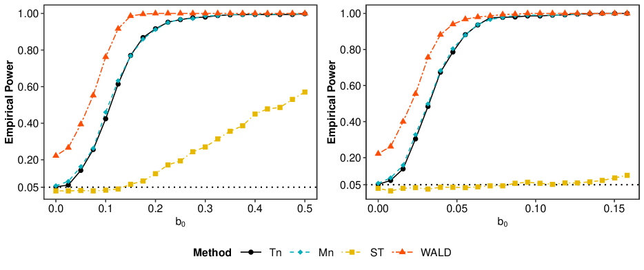
Figure 2: The left penal represents empirical sizes and powers of the $T_{n},M_{n}$, $ST$ and $WALD$ in the sparse alternative (setting 2). The right penal corresponds to dense alternative (setting 3). The solid line with circle points, dash line with diamond points, dot-dash line with square points and two-dash line with triangle points represent the empirical sizes and powers of $T_{n}$, $M_{n}$, $ST$ and $WALD$, respectively.

Table 1 reports the simulation results of scenario 2. We have the following observations. First, $T_{n}$ and $M_{n}$ control the type I error well, even when the dimension is $4000$. Second, the empirical powers increase when the dimension decreases and the sample size increases. Third, there is no significant difference in power between sparse and dense alternatives as long as $\lVert\bm{\beta}\rVert_{2}$ stays the same.

Table 1: The empirical type-I errors and powers for $T_{n}$ and $M_{n}$.

			Type-I Error			Power (Sparse)			Power (Dense)
$n$	$p$	$\rho$	$0.3$	$0.5$	$0.7$	$0.3$	$0.5$	$0.7$	$0.3$	$0.5$	$0.7$
$100$	$600$	$T_{n}$	$0.046$	$0.070$	$0.060$	$0.950$	$0.998$	$1.000$	$0.956$	$1.000$	$1.000$
		$M_{n}$	$0.050$	$0.058$	$0.054$	$0.964$	$0.998$	$1.000$	$0.950$	$1.000$	$1.000$
$100$	$1000$	$T_{n}$	$0.038$	$0.050$	$0.076$	$0.820$	$0.972$	$1.000$	$0.826$	$0.980$	$1.000$
		$M_{n}$	$0.042$	$0.050$	$0.076$	$0.808$	$0.974$	$1.000$	$0.824$	$0.980$	$1.000$
$100$	$2000$	$T_{n}$	$0.052$	$0.058$	$0.048$	$0.552$	$0.800$	$0.982$	$0.522$	$0.760$	$0.996$
		$M_{n}$	$0.042$	$0.062$	$0.042$	$0.532$	$0.796$	$0.984$	$0.504$	$0.780$	$0.990$
$100$	$4000$	$T_{n}$	$0.052$	$0.066$	$0.068$	$0.382$	$0.534$	$0.816$	$0.356$	$0.546$	$0.848$
		$M_{n}$	$0.046$	$0.066$	$0.064$	$0.376$	$0.516$	$0.826$	$0.348$	$0.528$	$0.852$
$200$	$600$	$T_{n}$	$0.048$	$0.056$	$0.060$	$1.000$	$1.000$	$1.000$	$1.000$	$1.000$	$1.000$
		$M_{n}$	$0.048$	$0.052$	$0.052$	$1.000$	$1.000$	$1.000$	$1.000$	$1.000$	$1.000$
$200$	$1000$	$T_{n}$	$0.062$	$0.062$	$0.054$	$1.000$	$1.000$	$1.000$	$1.000$	$1.000$	$1.000$
		$M_{n}$	$0.070$	$0.064$	$0.060$	$1.000$	$1.000$	$1.000$	$1.000$	$1.000$	$1.000$
$200$	$2000$	$T_{n}$	$0.070$	$0.048$	$0.068$	$0.982$	$1.000$	$1.000$	$0.978$	$0.998$	$1.000$
		$M_{n}$	$0.070$	$0.042$	$0.060$	$0.986$	$1,000$	$1.000$	$0.976$	$0.998$	$1.000$
$200$	$4000$	$T_{n}$	$0.040$	$0.050$	$0.052$	$0.818$	$0.956$	$1,000$	$0.796$	$0.986$	$1.000$
		$M_{n}$	$0.040$	$0.054$	$0.052$	$0.818$	$0.960$	$1,000$	$0.794$	$0.980$	$1.000$

• “Type-I error”, “Power (Sparse),” and “Power (Dense)” correspond to Setting 1, Setting two, and Setting 3.

Figure 3 displays the empirical size-power curves of $T_{n}$ and $M_{n}$ in scenario 3. We find that $T_{n}$ is too liberal to maintain the significance level. On the contrary, $M_{n}$ maintains the level well. As $b_{0}$ increases, although the empirical powers of $T_{n}$ and $M_{n}$ increase rapidly, the empirical power of $T_{n}$ does not go to $1$ as the increase of $b_{0}$. In contrast, the empirical power of $M_{n}$ can increase to 1 quickly. The results show that $M_{n}$ can also improve the power compared with $T_{n}$. This confirms the theory.

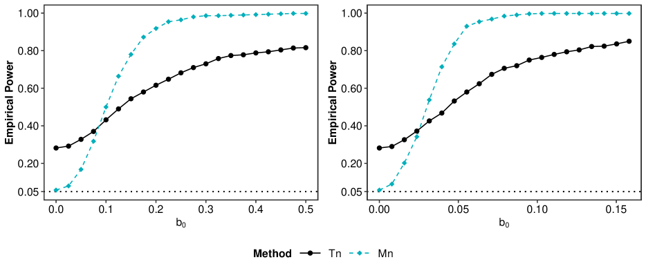
Figure 3: The left penal represents empirical sizes and powers of the $T_{n}$ and $M_{n}$ in the sparse alternatives (setting 2). The right penal corresponds to dense alternatives (setting 3). The solid line with circle points and dash line with diamond points represent the empirical sizes and powers of $T_{n}$ and $M_{n}$, respectively.

The above simulation studies conclude that our proposed tests perform well even when the testing and nuisance parameters are both ultrahigh dimensional. When a relatively high correlation exists between the covariates of interest and the nuisance covariates, $M_{n}$ can enhance the power performance over $T_{n}$. These confirm the merits of the orthogonalization technique.

6.2 Real data analysis

We apply our tests to a data set about riboflavin (vitamin B2) production rate with Bacillus Subtilis. This data set was made publicly by Bühlmann et al., (2014) and analyzed by several authors, for instance Van de Geer et al., (2014), Javanmard and Montanari, (2014), Dezeure et al., (2017), and Fei et al., (2019). It consists of $71$ observations of strains of Bacillus Subtilis and $4088$ covariates, measuring the log-expression levels of 4088 genes. The response variable is the logarithm of the riboflavin production rate.

First, we screen the covariates using the sure independence screening procedure in Fan and Lv, (2008). 133 genes are picked out using R-package SIS. Table LABEL:selectedgenesetofrealdata in the Supplementary Material reports the names of selected genes. Denote $\mathcal{G}$ as the selected gene set and $\mathcal{G}^{c}$ as its complement. The set $\mathcal{G}$ contains some detected genes reported in the literature, such as YXLD_at, YXLE_at, YCKE_at, and XHLA_at. A natural question is whether the selected genes contribute to the response given the other genes? Consider the following regression modeling:

$$Y=\bm{\beta}^{\top}\bm{V}_{\mathcal{G}}+\bm{\gamma}^{\top}\bm{V}_{\mathcal{G}^{c}}+\epsilon,$$

where $Y$ is the response variable, $\bm{V}_{\mathcal{G}}$ is the vector of selected genes, $\bm{V}_{\mathcal{G}^{c}}$ denotes the genes in set $\mathcal{G}^{c}$, and $\epsilon$ is the regression error. Further $\lVert\bm{\beta}\rVert_{0}=\lvert\mathcal{G}\rvert=133$, $\lVert\bm{\gamma}\rVert_{0}=\lvert\mathcal{G}^{c}\rvert=3955$. The null hypothesis of interest is $\mathbb{H}_{01}:\bm{\beta}=\bm{0}$. Thus the testing parameter is $\bm{\beta}$, and the nuisance parameter is $\bm{\gamma}$. The dimensions of $\bm{\beta}$ and $\bm{\gamma}$ are higher than the sample size ($n=71$). To verify whether some genes in $\mathcal{G}^{c}$ contribute to the response given the other genes, we also consider the null hypothesis $\mathbb{H}_{02}:\bm{\gamma}=\bm{0}$. In this testing problem $\mathbb{H}_{02}$, the testing parameter is changed to be $\bm{\gamma}$, and $\bm{\beta}$ is the nuisance parameter correspondingly.

Apply $T_{n}$, $M_{n}$, $ST$, and $WALD$. We standardize the data and report the $p$-values in Table 2. For the testing problem $\mathbb{H}_{01}$, only $T_{n}$ and $M_{n}$ reject the null hypothesis at the significance level $\alpha=0.01$. For the testing problem $\mathbb{H}_{02}$, all tests do not reject the null hypothesis at the significance level $\alpha=0.01$. The results suggest that the selected gene set $\mathcal{G}$ contributes to the response, and there is no significant gene in $\mathcal{G}^{c}$.

Table 2: The $p$-values for real data example.

Method	$T_{n}$	$M_{n}$	$ST$	$WALD$
	$p$-value
$\mathbb{H}_{01}$	0.008	$<$0.001	0.052	0.101
$\mathbb{H}_{02}$	0.794	0.789	0.402	0.377

7 Conclusions

This paper considers testing the significance of ultrahigh-dimensional parameter vector of interest with ultrahigh-dimensional nuisance parameter vector. We first reanalyze the score function-based test under weaker conditions to show the limiting distributions under the null and local alternative hypotheses. We construct an orthogonalized score function-based test to handle the correlation between the covariates of interest and nuisance covariates. Our investigation shows that the orthogonalization technique can debiase the error term, convert the non-degenerate error terms to degenerate, and reduce the variance to achieve higher power than the non-orthogonalized score function-based test.

Our procedure is very generic. Extensions to other regression models such as generalized linear regression models and partially linear regression models are possible. We would investigate these extensions in near future.

Appendix A Appendix

Notation. For functions $f(n)$ and $g(n)$, we write $f(n)\lesssim g(n)$ to mean that $f(n)\leq cg(n)$ for some universal constant $c\in(0,\infty)$, and similarly, $f(n)\gtrsim g(n)$ when $f(n)\geq c^{\prime}g(n)$ for some universal constant $c^{\prime}\in(0,\infty)$. We write $f(n)\asymp g(n)$ when $f(n)\lesssim g(n)$ and $f(n)\gtrsim g(n)$ hold simultaneously. The $\operatorname{\mathit{sub-Gaussian\ norm}}$ of a $\operatorname{\mathit{sub-Gaussian}}$ random variable $X$ is defined as $\lVert X\rVert_{\psi_{2}}{:=}\inf\{t>0:\mathbb{E}\exp(X^{2}/t^{2})\leq 2\}$. Similarly, the $\operatorname{\mathit{sub-Exponential\ norm}}$ of a $\operatorname{\mathit{sub-Exponential}}$ random variable $Y$ is defined as $\lVert Y\rVert_{\psi_{1}}{:=}\inf\{t>0:\,\mathbb{E}\exp(\lvert Y\rvert/t)\leq 2\}$. The $\operatorname{\mathit{sub-Gaussian\ norm}}$ of a $\operatorname{\mathit{sub-Gaussian}}$ random vector $X$ in $\mathbb{R}^{p}$ is defined as $\lVert{\bf{X}}\rVert_{\psi_{2}}:=\sup_{x\in\mathbb{S}^{p-1}}\lVert x^{\top}{\bf{X}}\rVert_{\psi_{2}}$. The $L_{p}$-$\mathit{norm}$ of a random variable $X$ in $\mathbb{R}$ is defined as $\lVert X\rVert_{p}:=(\mathbb{E}\lvert X\rvert^{p})^{1/p}$. For $x\in\mathbb{R}$, $\lceil x\rceil$ represents the least integer greater than or equal to $x$.

A.1 Proofs of Theorem 2.1

To save space we only present the proof of Theorem 2.1 here. The proofs of other theorems and related lemmas are put in the Supplementary Material. To simplify the representations of the proofs, we give nine lemmas in the Supplementary Material. Therefore, we will cite them in the proofs. For brevity, assume $\lVert\bm{\nu}\rVert_{\psi_{2}}=1$. To simplify the notation, let $\epsilon_{i}=Y_{i}-\bm{\gamma}^{\top}\mathbf{Z}_{i}$, $\widehat{\epsilon}_{i}=Y_{i}-\widehat{\bm{\gamma}}^{\top}\mathbf{Z}_{i}$ and $\breve{\bm{\gamma}}=\bm{\gamma}_{\phi}-\widehat{\bm{\gamma}}$.

As $\bm{\gamma}_{\phi}=\bm{\gamma}$ under $\mathbb{H}_{0}$, we decompose $T_{n}$ it as

$$T_{n} =\frac{1}{n}\sum_{i\neq j}\widehat{\epsilon}_{i}\widehat{\epsilon}_{j}{\bf{X}}_{i}^{\top}{\bf{X}}_{j}=\frac{1}{n}\sum_{i\neq j}(\epsilon_{i}+\breve{\bm{\gamma}}^{\top}\mathbf{Z}_{i})(\epsilon_{j}+\breve{\bm{\gamma}}^{\top}\mathbf{Z}_{j}){\bf{X}}_{i}^{\top}{\bf{X}}_{j}$$

$$=\frac{1}{n}\sum_{i\neq j}\epsilon_{i}\epsilon_{j}{\bf{X}}_{i}^{\top}{\bf{X}}_{j}+\frac{1}{n}\sum_{i\neq j}\breve{\bm{\gamma}}^{\top}\mathbf{Z}_{i}\breve{\bm{\gamma}}^{\top}\mathbf{Z}_{j}{\bf{X}}_{i}^{\top}{\bf{X}}_{j}$$

$$\quad\,\,+\frac{1}{n}\sum_{i\neq j}(\epsilon_{i}\breve{\bm{\gamma}}^{\top}\mathbf{Z}_{j}+\breve{\bm{\gamma}}^{\top}\mathbf{Z}_{i}\epsilon_{j}){\bf{X}}_{i}^{\top}{\bf{X}}_{j}$$

$$=:I_{1}^{\text{c}}+I_{2}^{\text{c}}+I_{3}^{\text{c}}.$$

Similar to the proof of Theorem 3 in Guo and Chen, (2016), we have

$$\frac{I_{1}^{\text{c}}}{\sqrt{2\Lambda_{{\bf{X}}}}}\rightarrow N(0,1)\quad\text{in distribution}$$

as $(n,p_{\bm{\beta}})\rightarrow\infty$. Lemma LABEL:lemma14 in the Supplementary Material gives the detailed proof about $I_{1}^{\text{c}}$. We now prove that $I_{2}^{\text{c}}$ and $I_{3}^{\text{c}}$ are $o_{p}(\sqrt{2\Lambda_{{\bf{X}}}})$.

Following Lemma LABEL:lemma37 in the Supplementary Material, we have

$$I_{2}^{\text{c}}\leq\biggl{\lVert}\frac{1}{n}\sum_{i\neq j}\mathbf{Z}_{i}\mathbf{Z}_{j}^{\top}{\bf{X}}_{i}^{\top}{\bf{X}}_{j}\biggr{\rVert}_{\infty}\lVert\breve{\bm{\gamma}}\rVert_{1}^{2},$$ (A.1)

Let $\mathbf{U}_{1}^{\text{c}}$ be a $p_{\bm{\gamma}}\times p_{\bm{\gamma}}$ dimension matrix with $(k_{1},k_{2})$-th element

$$U_{1,(k_{1},k_{2})}^{\text{c}}=\frac{1}{n}\sum_{i\neq j}\frac{1}{2}(Z_{i,k_{1}}Z_{j,k_{2}}+Z_{i,k_{2}}Z_{j,k_{1}}){\bf{X}}_{i}^{\top}{\bf{X}}_{j}.$$

Note that $\mathbf{U}_{1}^{\text{c}}=n^{-1}\sum_{i\neq j}\mathbf{Z}_{i}\mathbf{Z}_{j}^{\top}{\bf{X}}_{i}^{\top}{\bf{X}}_{j}$ and all of its elements are $U$-statistics. By Hoeffding decomposition, we derive

$$\frac{1}{n-1}U_{1,(k_{1},k_{2})}^{\text{c}}=\mathbb{E}(Z_{k_{1}}{\bf{X}})^{\top}\mathbb{E}(Z_{k_{2}}{\bf{X}})+2S_{1,1,(k_{1},k_{2})}^{\text{c}}+S_{1,2,(k_{1},k_{2})}^{\text{c}},$$

where

$$S_{1,1,(k_{1},k_{2})}^{\text{c}}=\frac{1}{n}\sum_{i=1}^{n}g_{1,1,(k_{1},k_{2})}^{\text{c}}({\bf{X}}_{i},\mathbf{Z}_{i})$$

with $g_{1,1,(k_{1},k_{2})}^{\text{c}}({\bf{X}}_{1},\mathbf{Z}_{1})=\{Z_{1,k_{1}}{\bf{X}}_{1}-\mathbb{E}(Z_{k_{1}}{\bf{X}})\}^{\top}\mathbb{E}(Z_{k_{2}}{\bf{X}})/2+\{Z_{1,k_{2}}{\bf{X}}_{1}-\mathbb{E}(Z_{k_{2}}{\bf{X}})\}^{\top}\mathbb{E}(Z_{k_{1}}{\bf{X}})/2$,

$$S_{1,2,(k_{1},k_{2})}^{\text{c}}=\frac{1}{n(n-1)}\sum_{i\neq j}^{n}g_{1,2,(k_{1},k_{2})}^{\text{c}}({\bf{X}}_{i},\mathbf{Z}_{i};{\bf{X}}_{j},\mathbf{Z}_{j})$$

with $g_{1,2,(k_{1},k_{2})}^{\text{c}}({\bf{X}}_{1},\mathbf{Z}_{1};{\bf{X}}_{2},\mathbf{Z}_{2})=\{Z_{1,k_{1}}{\bf{X}}_{1}-\mathbb{E}(Z_{k_{1}}{\bf{X}})\}^{\top}\{Z_{2,k_{2}}{\bf{X}}_{2}-\mathbb{E}(Z_{k_{2}}{\bf{X}})\}/2+\{Z_{1,k_{2}}{\bf{X}}_{1}-\mathbb{E}(Z_{k_{2}}{\bf{X}})\}^{\top}\{Z_{2,k_{1}}{\bf{X}}_{2}-\mathbb{E}(Z_{k_{1}}{\bf{X}})\}/2$.

For any $1\leq k_{1},k_{2}\leq p_{\bm{\gamma}}$, $Z_{1,k_{1}}$ is a sub-Gaussian random variable and $\mathbb{E}(Z_{k_{2}}{\bf{X}})^{\top}{\bf{X}}$ is a sub-Gaussian random variable with norm $\lVert\mathbb{E}(Z_{k_{2}}{\bf{X}})^{\top}{\bf{X}}\rVert_{\psi_{2}}\lesssim\{\mathbb{E}(Z_{k_{2}}{\bf{X}})^{\top}\bm{\Sigma}_{{\bf{X}}}\mathbb{E}(Z_{k_{2}}{\bf{X}})\}^{1/2}$. Thus $\{Z_{1,k_{1}}{\bf{X}}_{1}-\mathbb{E}(Z_{k_{1}}{\bf{X}})\}^{\top}\mathbb{E}(Z_{k_{2}}{\bf{X}})$ is sub-Exponential with norm

$$\lVert\{Z_{1,k_{1}}{\bf{X}}_{1}-\mathbb{E}(Z_{k_{1}}{\bf{X}})\}^{\top}\mathbb{E}(Z_{k_{2}}{\bf{X}})\rVert_{\psi_{1}} \leq\lVert Z_{1,k_{1}}\rVert_{\psi_{2}}\lVert\mathbb{E}(Z_{k_{2}}{\bf{X}})^{\top}{\bf{X}}\rVert_{\psi_{2}}$$

$$\lesssim\{\mathbb{E}(Z_{k_{2}}{\bf{X}})^{\top}\bm{\Sigma}_{{\bf{X}}}\mathbb{E}(Z_{k_{2}}{\bf{X}})\}^{1/2}.$$ (A.2)

Therefore we derive

$$\lVert\max_{1\leq i\leq n}\max_{1\leq k_{1},k_{2}\leq p_{\bm{\gamma}}}g_{1,1,(k_{1},k_{2})}^{\text{c}}\rVert_{2} \lesssim\log(np_{\bm{\gamma}})\max_{1\leq i\leq n}\max_{1\leq k_{1},k_{2}\leq p_{\bm{\gamma}}}\lVert g_{1,1,(k_{1},k_{2})}^{\text{c}}\rVert_{\psi_{1}}$$

$$\lesssim\log(np_{\bm{\gamma}})\max_{1\leq k\leq p_{\bm{\gamma}}}\{\mathbb{E}(Z_{k}{\bf{X}})^{\top}\bm{\Sigma}_{{\bf{X}}}\mathbb{E}(Z_{k}{\bf{X}})\}^{1/2}$$

$$\lesssim\log(np_{\bm{\gamma}})\lambda_{\rm{max}}^{1/2}(\bm{\Sigma}_{{\bf{X}}})\varrho.$$ (A.3)

The first inequality follows from Lemma LABEL:lemma36 in the Supplementary Material. The second inequality holds by inequality (A.1).

Denote $q=\lceil 4/(1-3b)\rceil$. We have

$$\lVert\max_{1\leq i\neq j\leq n}\max_{1\leq k_{1},k_{2}\leq p_{\bm{\gamma}}}g_{1,2,(k_{1},k_{2})}^{\text{c}}\rVert_{4} \leq\lVert\max_{1\leq i\neq j\leq n}\max_{1\leq k_{1},k_{2}\leq p_{\bm{\gamma}}}g_{1,2,(k_{1},k_{2})}^{\text{c}}\rVert_{q}$$

$$\lesssim\lVert\max_{1\leq i\neq j\leq n}\max_{1\leq k_{1},k_{2}\leq p_{\bm{\gamma}}}Z_{i,k_{1}}Z_{j,k_{2}}{\bf{X}}_{i}^{\top}{\bf{X}}_{j}\rVert_{q}$$

$$\lesssim\lVert\max_{1\leq i\neq j\leq n}\max_{1\leq k_{1},k_{2}\leq p_{\bm{\gamma}}}Z_{i,k_{1}}Z_{j,k_{2}}\rVert_{2q}\lVert\max_{1\leq i\neq j\leq n}{\bf{X}}_{i}^{\top}{\bf{X}}_{j}\rVert_{2q}$$

$$\lesssim\log(np_{\bm{\gamma}})\max_{1\leq k_{1},k_{2}\leq p_{\bm{\gamma}}}\lVert Z_{1,k_{1}}Z_{2,k_{2}}\rVert_{\psi_{1}}n^{1/q}\mathrm{tr}^{1/2}(\bm{\Sigma}_{{\bf{X}}}^{2})$$

$$\lesssim\log(np_{\bm{\gamma}})n^{1/q}\mathrm{tr}^{1/2}(\bm{\Sigma}_{{\bf{X}}}^{2}).$$ (A.4)

The first inequality holds by Liapounov inequality. The third inequality holds by Cauchy-Schwartz inequality, the fourth inequality holds by the property of Orlicz norm(Page 96 in Van der Vaart and Wellner, (1996)), Lemmas LABEL:lemma36 and LABEL:lemmaofassumptionb5 in the Supplementary Material. The last inequality holds by Assumption 2.2. Similarly, we derive

$$\max_{1\leq k_{1},k_{2}\leq p_{\bm{\gamma}}}\lVert g_{1,1,(k_{1},k_{2})}^{\text{c}}\rVert_{2}\lesssim\lambda_{\rm{max}}^{1/2}(\bm{\Sigma}_{{\bf{X}}})\varrho$$ (A.5)

and

$$\max_{1\leq k_{1},k_{2}\leq p_{\bm{\gamma}}}\lVert g_{1,2,(k_{1},k_{2})}^{\text{c}}\rVert_{2}\leq\max_{1\leq k_{1},k_{2}\leq p_{\bm{\gamma}}}\lVert g_{1,2,(k_{1},k_{2})}^{\text{c}}\rVert_{4}\lesssim\mathrm{tr}^{1/2}(\bm{\Sigma}_{{\bf{X}}}^{2}).$$ (A.6)

Applying Lemma LABEL:lemma26 in the Supplementary Material, we derive

$$\mathbb{E}(\lVert\mathbf{U}_{1}^{\text{c}}\rVert_{\infty})\lesssim n\varrho^{2}+\{n^{1/2}(\log p_{\bm{\gamma}})^{1/2}+\log p_{\bm{\gamma}}\log(np_{\bm{\gamma}})\}\lambda_{\rm{max}}^{1/2}(\bm{\Sigma}_{{\bf{X}}})\varrho$$

$$+\{\log p_{\bm{\gamma}}+n^{-1/2+1/q}(\log p_{\bm{\gamma}})^{3/2}\log(np_{\bm{\gamma}})\}\mathrm{tr}^{1/2}(\bm{\Sigma}_{{\bf{X}}}^{2})$$

$$\lesssim n\varrho^{2}+n^{1/2}(\log p_{\bm{\gamma}})^{1/2}\lambda_{\rm{max}}^{1/2}(\bm{\Sigma}_{{\bf{X}}})\varrho+\log p_{\bm{\gamma}}\mathrm{tr}^{1/2}(\bm{\Sigma}_{{\bf{X}}}^{2}),$$ (A.7)

where the first inequality holds by Lemma LABEL:lemma26 in the Supplementary Material and the inequalities (A.1)-(A.6). The last inequality holds by the fact $\log p_{\bm{\gamma}}=O(n^{b})$, where $0<b<1/3$. Combining equations (A.1) and (A.1), Assumption 2.3, we have

$$I_{2}^{\text{c}}=O_{p}\bigl{\{}s^{2}\log p_{\bm{\gamma}}\varrho^{2}+n^{-1/2}s^{2}(\log p_{\bm{\gamma}})^{3/2}\lambda_{\rm{max}}^{1/2}(\bm{\Sigma}_{{\bf{X}}})\varrho+n^{-1}s^{2}(\log p_{\bm{\gamma}})^{2}\mathrm{tr}^{1/2}(\bm{\Sigma}_{{\bf{X}}}^{2})\bigr{\}}.$$ (A.8)

Thus $I_{2}^{\text{c}}=o_{p}(\sqrt{\Lambda_{{\bf{X}}}})$ when $s^{2}\log p_{\bm{\gamma}}\varrho^{2}=o(\sqrt{\Lambda_{{\bf{X}}}})$, $n^{-1/2}s^{2}(\log p_{\bm{\gamma}})^{3/2}\lambda_{\rm{max}}^{1/2}(\bm{\Sigma}_{{\bf{X}}})\varrho=o(\sqrt{\Lambda_{{\bf{X}}}})$ and $n^{-1}s^{2}(\log p_{\bm{\gamma}})^{2}=o(1)$ hold simultaneously.

Similar to the proof of $I_{2}^{\text{c}}$, we derive

$$I_{3}^{\text{c}}\leq\biggl{\lVert}\frac{1}{n}\sum_{i\neq j}(\epsilon_{i}\mathbf{Z}_{j}+\mathbf{Z}_{i}\epsilon_{j}){\bf{X}}_{i}^{\top}{\bf{X}}_{j}\biggr{\rVert}_{\infty}\lVert\breve{\bm{\gamma}}\rVert_{1}.$$ (A.9)

Let $\mathbf{U}_{2}^{\text{c}}$ be a $p_{\bm{\gamma}}$ dimension vector with $k$-th element

$$U_{2,k}^{\text{c}}=\frac{1}{n}\sum_{i\neq j}(\epsilon_{i}Z_{j,k}+Z_{i,k}\epsilon_{j}){\bf{X}}_{i}^{\top}{\bf{X}}_{j}.$$

Note that $\mathbf{U}_{2}^{\text{c}}=n^{-1}\sum_{i\neq j}(\epsilon_{i}\mathbf{Z}_{j}+\mathbf{Z}_{i}\epsilon_{j}){\bf{X}}_{i}^{\top}{\bf{X}}_{j}$ and all of its elements are $U$-statistics. By Hoeffding decomposition again, we derive

$$\frac{1}{n-1}U_{2,k}^{\text{c}}=2S_{2,1,k}^{\text{c}}+S_{2,2,k}^{\text{c}},$$

where

$$S_{2,1,k}^{\text{c}}=\frac{1}{n}\sum_{i=1}^{n}g_{2,1,k}^{\text{c}}({\bf{X}}_{i},\mathbf{Z}_{i},\epsilon_{i})$$

with $g_{2,1,k}^{\text{c}}({\bf{X}}_{1},\mathbf{Z}_{1},\epsilon_{1})=\epsilon_{1}{\bf{X}}_{1}^{\top}\mathbb{E}(Z_{k}{\bf{X}})$,

$$S_{2,2,k}^{\text{c}}=\frac{1}{n(n-1)}\sum_{i\neq j}^{n}g_{2,2,k}^{\text{c}}({\bf{X}}_{i},\mathbf{Z}_{i},\epsilon_{i};{\bf{X}}_{j},\mathbf{Z}_{j},\epsilon_{j})$$

with $g_{2,2,k}^{\text{c}}({\bf{X}}_{i},\mathbf{Z}_{i},\epsilon_{i};{\bf{X}}_{j},\mathbf{Z}_{j},\epsilon_{j})=\epsilon_{1}{\bf{X}}_{1}^{\top}\{Z_{2,k}{\bf{X}}_{2}-\mathbb{E}(Z_{k}{\bf{X}})\}+\epsilon_{2}{\bf{X}}_{2}^{\top}\{Z_{1,k}{\bf{X}}_{1}-\mathbb{E}(Z_{k}{\bf{X}})\}$.

Similar to the proof of inequality (A.1), we derive

$$\lVert\max_{1\leq i\leq n}\max_{1\leq k\leq p_{\bm{\gamma}}}g_{2,1,k}^{\text{c}}\rVert_{2} \lesssim\lVert\max_{1\leq i\leq n}\max_{1\leq k\leq p_{\bm{\gamma}}}\epsilon_{i}{\bf{X}}_{i}^{\top}\mathbb{E}(Z_{k}{\bf{X}})\rVert_{2}$$

$$\lesssim\log(np_{\bm{\gamma}})\max_{1\leq k\leq p_{\bm{\gamma}}}\lambda_{\rm{max}}^{1/2}(\bm{\Sigma}_{{\bf{X}}})\varrho.$$ (A.10)

The last inequality is derived by Assumption 2.5, Lemma LABEL:lemma36 in the Supplementary Material, and the technique used in the last inequality in the proof for the inequality (A.1). Similar to the proof of (A.1), we derive

$$\lVert\max_{1\leq i\neq j\leq n}\max_{1\leq k\leq p_{\bm{\gamma}}}g_{2,2,k}^{\text{c}}\rVert_{4} \leq\lVert\max_{1\leq i\neq j\leq n}\max_{1\leq k\leq p_{\bm{\gamma}}}g_{2,2,k}^{\text{c}}\rVert_{q}$$

$$\lesssim\lVert\max_{1\leq i\neq j\leq n}\max_{1\leq k\leq p_{\bm{\gamma}}}\epsilon_{1}Z_{2,k}{\bf{X}}_{1}^{\top}{\bf{X}}_{2}\rVert_{q}$$

$$\lesssim\log(np_{\bm{\gamma}})n^{1/q}\mathrm{tr}^{1/2}(\bm{\Sigma}_{{\bf{X}}}^{2}).$$ (A.11)

Similarly,

$$\max_{1\leq k\leq p_{\bm{\gamma}}}\lVert g_{2,1,k}^{\text{c}}\rVert_{2}\lesssim\lambda_{\rm{max}}(\bm{\Sigma}_{{\bf{X}}})\varrho^{2}$$ (A.12)

and

$$\max_{1\leq k\leq p_{\bm{\gamma}}}\lVert g_{2,2,k}^{\text{c}}\rVert_{2}\leq\max_{1\leq k\leq p_{\bm{\gamma}}}\lVert g_{2,2,k}^{\text{c}}\rVert_{4}\lesssim\mathrm{tr}^{1/2}(\bm{\Sigma}_{{\bf{X}}}^{2}).$$ (A.13)

The argument for proving the inequality (A.1) yields

$$\mathbb{E}(\lVert\mathbf{U}_{2}^{\text{c}}\rVert_{\infty})\lesssim n^{1/2}(\log p_{\bm{\gamma}})^{1/2}\lambda_{\rm{max}}^{1/2}(\bm{\Sigma}_{{\bf{X}}})\varrho+\log p_{\bm{\gamma}}\mathrm{tr}^{1/2}(\bm{\Sigma}_{{\bf{X}}}^{2}).$$ (A.14)

Combining equations (A.9) and (A.14), Assumption 2.3, we have

$$I_{3}^{\text{c}}=O_{p}\bigl{\{}s\log p_{\bm{\gamma}}\lambda_{\rm{max}}^{1/2}(\bm{\Sigma}_{{\bf{X}}})\varrho+n^{-1/2}s(\log p_{\bm{\gamma}})^{3/2}\mathrm{tr}^{1/2}(\bm{\Sigma}_{{\bf{X}}}^{2})\bigr{\}}.$$ (A.15)

Thus $I_{3}^{\text{c}}=o_{p}(\sqrt{\Lambda_{{\bf{X}}}})$ when $s\log p_{\bm{\gamma}}\lambda_{\rm{max}}^{1/2}(\bm{\Sigma}_{{\bf{X}}})\varrho=o(\sqrt{\Lambda_{{\bf{X}}}})$ and $n^{-1/2}s(\log p_{\bm{\gamma}})^{3/2}=o(1)$ hold simultaneously. The proof is concluded.

References

- Bai and Saranadasa, (1996) Bai, Z. and Saranadasa, H. (1996). Effect of high dimension: by an example of a two sample problem. Statistica Sinica, 6(2):311–329.
- Belloni et al., (2012) Belloni, A., Chen, D., Chernozhukov, V., and Hansen, C. (2012). Sparse models and methods for optimal instruments with an application to eminent domain. Econometrica, 80(6):2369–2429.
- Belloni et al., (2018) Belloni, A., Chernozhukov, V., Chetverikov, D., and Wei, Y. (2018). Uniformly valid post-regularization confidence regions for many functional parameters in z-estimation framework. Annals of statistics, 46(6B):3643–3675.
- Belloni et al., (2015) Belloni, A., Chernozhukov, V., and Kato, K. (2015). Uniform post-selection inference for least absolute deviation regression and other z-estimation problems. Biometrika, 102(1):77–94.
- Bühlmann et al., (2014) Bühlmann, P., Kalisch, M., and Meier, L. (2014). High-dimensional statistics with a view toward applications in biology. Annual Review of Statistics and Its Application, 1(1):255–278.
- Cai and Guo, (2020) Cai, T. and Guo, Z. (2020). Semisupervised inference for explained variance in high dimensional linear regression and its applications. Journal of the Royal Statistical Society: Series B (Statistical Methodology), 82(2):391–419.
- Candes et al., (2018) Candes, E., Fan, Y., Janson, L., and Lv, J. (2018). Panning for gold:‘model-x’knockoffs for high dimensional controlled variable selection. Journal of the Royal Statistical Society: Series B (Statistical Methodology), 80(3):551–577.
- Chen et al., (2022) Chen, J., Li, Q., and Chen, H. Y. (2022). Testing generalized linear models with high-dimensional nuisance parameters. Biometrika, In press.
- Chen et al., (2009) Chen, S. X., Peng, L., and Qin, Y.-L. (2009). Effects of data dimension on empirical likelihood. Biometrika, 96(3):711–722.
- Chen and Qin, (2010) Chen, S. X. and Qin, Y.-L. (2010). A two-sample test for high-dimensional data with applications to gene-set testing. Annals of Statistics, 38(2):808–835.
- Chen, (2018) Chen, X. (2018). Gaussian and bootstrap approximations for high-dimensional u-statistics and their applications. Annals of Statistics, 46(2):642–678.
- Chernozhukov et al., (2018) Chernozhukov, V., Chetverikov, D., Demirer, M., Duflo, E., Hansen, C., Newey, W., and Robins, J. (2018). Double/debiased machine learning for treatment and structural parameters. The Econometrics Journal, 21(1):C1–C68.
- Chernozhukov et al., (2015) Chernozhukov, V., Chetverikov, D., and Kato, K. (2015). Comparison and anti-concentration bounds for maxima of gaussian random vectors. Probability Theory and Related Fields, 162(1):47–70.
- Cui et al., (2018) Cui, H., Guo, W., and Zhong, W. (2018). Test for high-dimensional regression coefficients using refitted cross-validation variance estimation. Annals of Statistics, 46(3):958–988.
- Dezeure et al., (2017) Dezeure, R., Bühlmann, P., and Zhang, C.-H. (2017). High-dimensional simultaneous inference with the bootstrap. Test, 26(4):685–719.
- Fan and Lv, (2008) Fan, J. and Lv, J. (2008). Sure independence screening for ultrahigh dimensional feature space. Journal of the Royal Statistical Society: Series B (Statistical Methodology), 70(5):849–911.
- Fei et al., (2019) Fei, Z., Zhu, J., Banerjee, M., and Li, Y. (2019). Drawing inferences for high-dimensional linear models: A selection-assisted partial regression and smoothing approach. Biometrics, 75(2):551–561.
- Goeman et al., (2006) Goeman, J. J., Van De Geer, S. A., and Van Houwelingen, H. C. (2006). Testing against a high dimensional alternative. Journal of the Royal Statistical Society: Series B (Statistical Methodology), 68(3):477–493.
- Guo and Chen, (2016) Guo, B. and Chen, S. X. (2016). Tests for high dimensional generalized linear models. Journal of the Royal Statistical Society: Series B (Statistical Methodology), 78(5):1079–1102.
- Guo et al., (2022) Guo, W., Zhong, W., Duan, S., and Cui, H. (2022). Conditional test for ultrahigh dimensional linear regression coefficients. Statistica Sinica, 32(3):1381–1409.
- Guo et al., (2021) Guo, Z., Renaux, C., Bühlmann, P., and Cai, T. (2021). Group inference in high dimensions with applications to hierarchical testing. Electronic Journal of Statistics, 15(2):6633–6676.
- Javanmard and Montanari, (2014) Javanmard, A. and Montanari, A. (2014). Confidence intervals and hypothesis testing for high-dimensional regression. Journal of Machine Learning Research, 15(1):2869–2909.
- Loh and Wainwright, (2015) Loh, P.-L. and Wainwright, M. J. (2015). Regularized m-estimators with nonconvexity: Statistical and algorithmic theory for local optima. Journal of Machine Learning Research, 16(1):559–616.
- Ma et al., (2021) Ma, R., Tony Cai, T., and Li, H. (2021). Global and simultaneous hypothesis testing for high-dimensional logistic regression models. Journal of the American Statistical Association, 116(534):984–998.
- Ning and Liu, (2017) Ning, Y. and Liu, H. (2017). A general theory of hypothesis tests and confidence regions for sparse high dimensional models. Annals of Statistics, 45(1):158–195.
- Serfling, (1980) Serfling, R. J. (1980). Approximation theorems of mathematical statistics. John Wiley & Sons.
- Sun and Zhang, (2012) Sun, T. and Zhang, C.-H. (2012). Scaled sparse linear regression. Biometrika, 99(4):879–898.
- Van de Geer et al., (2014) Van de Geer, S., Bühlmann, P., Ritov, Y., and Dezeure, R. (2014). On asymptotically optimal confidence regions and tests for high-dimensional models. Annals of Statistics, 42(3):1166–1202.
- Van der Vaart and Wellner, (1996) Van der Vaart, A. W. and Wellner, J. A. (1996). Weak Convergence and Empirical Processes: With Applications to Statistics. Springer, New York.
- Wainwright, (2019) Wainwright, M. J. (2019). High-Dimensional Statistics: A Non-Asymptotic Viewpoint. Cambridge University Press.
- Wu et al., (2021) Wu, Y., Wang, L., and Fu, H. (2021). Model-assisted uniformly honest inference for optimal treatment regimes in high dimension. Journal of the American Statistical Association, In press.
- Zhang and Zhang, (2014) Zhang, C.-H. and Zhang, S. S. (2014). Confidence intervals for low dimensional parameters in high dimensional linear models. Journal of the Royal Statistical Society: Series B (Statistical Methodology), 76(1):217–242.
- Zhang and Cheng, (2017) Zhang, X. and Cheng, G. (2017). Simultaneous inference for high-dimensional linear models. Journal of the American Statistical Association, 112(518):757–768.
- Zhong and Chen, (2011) Zhong, P.-S. and Chen, S. X. (2011). Tests for high-dimensional regression coefficients with factorial designs. Journal of the American Statistical Association, 106(493):260–274.
- Zhu and Xue, (2006) Zhu, L. and Xue, L. (2006). Empirical likelihood confidence regions in a partially linear single-index model. Journal of the Royal Statistical Society: Series B (Statistical Methodology), 68(3):549–570.