Statistically consistent inverse optimal control for discrete-time indefinite linear-quadratic systems
Abstract
The Inverse Optimal Control (IOC) problem is a structured system identification problem that aims to identify the underlying objective function based on observed optimal trajectories. This provides a data-driven way to model experts’ behavior. In this paper, we consider the case of discrete-time finite-horizon linear-quadratic problems where: the quadratic cost term in the objective is not necessarily positive semi-definite; the planning horizon is a random variable; we have both process noise and observation noise; the dynamics can have a drift term; and where we can have a linear cost term in the objective. In this setting, we first formulate the necessary and sufficient conditions for when the forward optimal control problem is solvable. Next, we show that the corresponding IOC problem is identifiable. Using the optimality conditions of the forward problem, we then formulate an estimator for the parameters in the objective function of the forward problem as the globally optimal solution to a convex optimization problem, and prove that the estimator is statistical consistent. Finally, the performance of the algorithm is demonstrated on a numerical example.
keywords:
Inverse optimal control, Indefinite linear quadratic regulator, System identification, Time-varying system matrices, Convex optimization, Semidefinite programming, Inverse reinforcement learning,
1 Introduction
Optimal control is a powerful framework in which control decisions are performed in order to minimize some given objective function; see, e.g., one of the monographs [anderson2007optimal, bertsekas2000dynamic]. In fact, many processes in nature can be model as optimal control problems with respect to some criteria [alexander1996optima]. However, in applications of optimal control, a fundamental problem is to design an appropriate objective function. In order to induce an appropriate control response, the object function needs to be adapted to the contextual environment in which the system is operating. This is a difficult task, which relies heavily on the designers’ experience and imagination.
Instead of designing the cost criteria, one way to overcome this difficulty would be to identify the cost function from the observations of an expert system that behaves “optimally” in the environment and thus “imitating” the expert behaviour. The latter is known as Inverse Optimal Control (IOC) [kalman1964linear], and has received considerable attention. In particular, IOC reconstructs the objective function of the expert system and hence predicts the closed-loop system’s behaviour using observed data as well as the knowledge of underlying system dynamics. The problem can be categorized as gray-box system identification [ljung1999system, p. 13], and is also closely related to inverse reinforcement learning [ng2000algorithms].
As one of the most classical optimal controller designs, linear-quadratic optimal regulators has been widely used in engineering. Though most of the literature considers the case of (the penalty parameter for the states) being positive semi-definite, indefinite linear-quadratic optimal control [chen1998stochastic, ran1993linear, rami2002discrete, ferrante2015note, ferrante2016discussion] has found applications in, e.g., mathematical finance [zhou2000continuous], crowd evacuation [toumi2020tractable, toumi2021spatial], and controller design for automatic steering of ships [reid1983optimal]. To this end, we are motivated to develop an IOC framework for general indefinite linear-quadratic optimal control. Linear-quadratic IOC problem has been studied under many different settings, including the infinite-horizon case in both continuous time [boyd1994linear, anderson2007optimal] and discrete time [priess2014solutions], respectively, as well as the finite-horizon case in both continuous time [li2018convex, li2020continuous] and discrete time [keshavarz2011imputing, zhang2019inverse, yu2021system, zhang2021inverse, zhang2022statistically], respectively. IOC is also closely connected to inverse reinforcement learning [ng2000algorithms], and this perspective has been used in [xue2021inverse, lian2021robust, xue2021inverse_tracking] to consider infinite horizon discrete-time and continuous-time linear-quadratic set-ups for regulation, tracking, and adversary scenarios, respectively. However, to the best of our knowledge, IOC frameworks for general indefinite linear-quadratic optimal control has not been considered yet. Furthermore, there are also other important aspects that have not been fully investigated in the aforementioned literature. More precisely, any real-world data would inevitably contain noise: it can either be process noise, observation noise, or both. Therefore, from robustness and accuracy perspectives, it is important to have a statistically consistent estimator, i.e., that converges to the true underlying parameter values as the number of observation grows. Moreover, many of the aforementioned IOC algorithms that are based on optimization either suffer from the fact that the estimation problems are nonconvex [keshavarz2011imputing, zhang2019inverse, yu2021system], and can therefore have issues with local minima, or suffer from the fact the estimation procedure needs to know the control gain a priori [boyd1994linear, anderson2007optimal, priess2014solutions, li2018convex, li2020continuous]. In the latter case, the estimation normally needs to be done in a two-stage procedure and the information is thus not used in the most efficient way. Furthermore, most of the literature on linear-quadratic IOC consider the regulation problem. However, in many experimental set-ups, an expert agent may have more complicated tasks than regulation, e.g., tracking a reference signal. Finally, real-world data can be of different time lengths, and this needs to be handled in a systematic way in order not to deteriorate the estimates.
In this work, we address these issues. More specifically, we consider the generalized linear-quadratic, indefinite, discrete-time IOC problem. We extend our previous work [zhang2021inverse] where we consider the standard linear-quadratic IOC problem for indistinguishable agents only with noisy measurements and fixed time-horizon length. We also extend the conference paper [zhang2022statistically], where we only considered the linear-quadratic positive semi-definite tracking case with random planning horizons. In particular, the contribution of this work is three-fold:
-
1.
We give necessary and sufficient conditions for the well-posedness of the generalized discrete-time finite-horizon indefinite linear-quadratic optimal control problem. Specifically, we do not assume that the running cost is positive semi-definite, and we include a linear term in the objective function, a forcing term in the dynamics, and process noise.
-
2.
We prove the identifiability of the parameters in the objective function.
-
3.
We construct an IOC algorithm that works for both the positive semi-definite and the indefinite case. The algorithm is based on convex optimization, and we show that its unique optimal solution is the “true” underlying parameters in the objective function of the forward problem. Moreover, the constructed optimization problem is approximated by empirical mean in practice and we also show that the estimator based on the approximated optimization is statistically consistent. This means that the estimator converge in probability to the true underlying parameter when the number of observations goes to infinity. In addition, the convex optimization formulation guarantees that the statistically consistent estimate that corresponds to the global optimum can actually be attained in practice.
The article is organized as follows. In Section 2, we formulate the forward and inverse problem, and specify the assumptions we use. Next, in Section 3, we analyze the forward problem and prove the necessary and sufficient conditions for when it is well-posed. Section 4 investigates the identifiability issue of the formulated IOC problem, and in particular prove that the formulated IOC problem is identifiable. In Section 5, we construct the IOC algorithm, construct the estimator, and prove that the latter is statistical consistent. To illustrate the performance of the proposed algorithm, in Section 6 we include a numerical example. Finally, we conclude the paper in Section 7. For improved readability, some proofs are deferred to the Appendix.
Notation: denotes the set of symmetric matrices, while denotes the set of positive semi-definite matrices. denotes -norm and denotes Frobenius norm. denotes the open ball of radius centered at , and denotes its closure. Moreover, . For , we denote as Loewner partial order of and , i.e., . Further, denotes the Moore-Penrose pseudo-inverse of . For integers , we let denote , and define the expression as empty if . In addition, by and we denote the image space and kernel, respectively, by ⟂ we denote the orthogonal complement, and by we denote the (mathematical) negation of a statement. Finally, we use italic bold font to denote stochastic elements, and use to denote convergence in probability, i.e., for a sequence of random elements and a random element , means that for all , .
2 Problem formulation
We start by introducing the mathematical formulation of the forward optimal control problem. To this end, let be a probability space that carries random vectors , , , and a random variable . It is assumed that for each realization of the random element (corresponding to the initial position and planning horizon length), the agent’s control decision is determined by a stochastic generalized linear-quadratic control problem, namely,
| (1a) | ||||
| s.t. | ||||
| (1b) | ||||
| (1c) | ||||
| (1d) | ||||
| (1e) | ||||
where , , , , and . More specifically, the minimization in (1) is over admissible control strategies with complete state information, i.e., is a function that maps from to , (see, e.g., [astrom1970introduction, Chp. 8]). Furthermore, the reason why we only consider a time-invariant external forcing term in (1b) is to simplify the presentation. The results of the paper also hold for time-varying forcing terms , provided that the agent knows all the future forcing terms for . Similarly, this formulation can be extended to tracking-problems by letting the linear cost term be time-varying, where is the reference signal, and the results in the paper follows analogously (cf. [zhang2022statistically]). In addition, we will in general make the following assumptions.
Assumption 2.1 (Controlability and full rank).
The system is controllable, is invertible, and is of full-column rank.
Assumption 2.2 (I.I.D. random variables).
The random elements , , are mutually independent. In addition, the random vectors are identically distributed (I.I.D.), the random vectors are I.I.D., , , , and , , where and are a priori known.
The rationale behind the first assumption is that we are considering a controllable discrete-time linear system that is not over-actuated, and that is sampled from a continuous-time system.
The formulation (1) is motivated by the fact that an agent can have different time horizon lengths (and initial values) to complete different tasks, while the underlying decision principle (i.e., running cost) remains unchanged since the principle is connected to the agent’s characteristics. In particular, given a realization of the time-horizon length and initial value , the agent starts to apply its control from the initial value at the time instant and the agent maintains the same running cost for each control execution. This formulation gives a systematic way to handle real-world data with different time lengths (see [zhang2022statistically]). However, due to the fact that might not be positive semi-definite, (1) might not admit an optimal solution (see, e.g. [ferrante2015note, ferrante2016discussion]). We analyze the well-posedness of the forward problem (1) in depth in Section 3. To proceed, we first make the following mild assumptions regarding the stochastic planning horizon .
Assumption 2.3 (Support of the planning horizon).
The constant is known, and . Moreover, the probability distribution for satisfies , and .
The above assumption means that the longest possible planning horizon is known, that it is sufficiently long, and that the longest horizon can be realized, i.e., it has a nonzero probability. In addition, we have the following proposition which illustrates the reason why we emphasize the longest time-horizon length in Assumption 2.3.
Proposition 2.4.
Proof.
See appendix. ∎
With Assumption 2.3 and Proposition 2.4 in mind, we are thus interested in parameters that belong to the following set:
| (1) with the objective function given by admits | ||
| solutions a.s. under the distribution of and for all | ||
More specifically, if , then the forward problem is well-posed for any under the distribution of almost surely. In addition, for the inverse problem we assume that the observation of the optimal states are contaminated by observation noise:
| (2) |
and that we observe trials of the agent. More precisely, let have the same distribution as , for all and all . Then the observed trajectories of the agent’s trials, , are just realizations of the I.I.D. random vectors .
Before we formulate the IOC problem, we also make the following assumptions.
Assumption 2.5 (Persistent excitation).
The random element is such that . Moreover, for all such that , the conditional distribution is such that for all there exists a such that for all .
Assumption 2.6 (Bounded parameters).
The parameter tuple that governs the agents tracking behaviour lies in the compact set
for some (potentially unknown) .
When we solve the corresponding inverse problem in practice, we can always set arbitrary large if we have no prior knowledge on the norm bound of the parameters. With the setup presented in this section, we summarize the IOC problem to be considered in this paper. For the sake of simplicity, we consider the case when designing the IOC algorithm.
3 Forward problem analysis
Before we present the IOC algorithm set-up, we first need to analyze the forward problem. More precisely, we need to characterize the set and find the necessary and sufficient optimality conditions for the existence of such generalized indefinite linear-quadratic optimal control. This is not only because we want to ensure that the forward-problem is well-behaved, but also to construct the IOC algorithm based on the optimality conditions. Moreover, we also analyze the properties of the time-varying closed-loop system matrices that will be useful in developing the IOC algorithm. For the theoretical development in this section, we do not assume that .
3.1 Necessary and sufficient conditions for existence of optimal control
To this end, we first derive the necessary and sufficient conditions for existence of optimal control to (1). The results build on [ferrante2015note]; in particular, some of the proof ideas are inspired by the proof in [ferrante2015note, Thm. 2.1]. However, we not only extend the result to a more general setting of stochastic linear-quadratic problems, but also show that solvability of the forward problem, i.e., that , can be characterized in different, but equivalent, ways. The main result of this section is the following.
Theorem 3.1 (Boundedness of forward problem).
Under Assumptions 2.2 and 2.5, the following statements are equivalent:
-
1.
.
-
2.
Let and be generated by the following Riccati iterations
(3a) (3b) (3c) (3d) Denote
(4a) (4b) (4c) It holds that (4d) (4e) for all .
- 3.
- 4.
In addition, if any of the four above conditions hold, then the optimal control signal for (1) is parametrized by any arbitrary vector , and is given by
| (9a) | ||||
| (9b) | ||||
where is the projection operator onto the kernel space of .111For the fact that is indeed the projection operator onto the kernel space of , see, e.g., [engl2000regularization, Prop. 2.3].
Proof.
First, assume that 4) holds. Note that for an agent with a planning horizon realization , by the principle of optimality in dynamic programming (see, e.g., [bertsekas2000dynamic, p. 18]), we can easily show that 4)1) (cf. [bertsekas2000dynamic, Prop. 1.3.1]). For the case , note that the HJBE is still valid for , and thus the agents behavior is still optimal in . Since the systems behavior for is completely determined by (1c), and (1e), by Bellman’s principle of optimality, the solution to the HJBE still gives the optimal control. This implies 1), and hence shows that 4)1).
Next, we prove that 1)2) by proving the contraposition of the statement, i.e., by proving that 2) 1). Before we proceed, first note the fact that
| (10) |
for any . Taking the expectation with respect to on both sides of (10), adding the latter expression to (1a), and using (1b), (3a), (3c), and Assumption 2.2, we can write the objective function as
| (11) |
with in the form of (5b) and in . Note that the term in the above equation is constant with respect to the state and the control and hence can be discarded in the optimization problem. On the other hand, since and are generated by (3), can also be written as
| (12) |
Now, we use the above trick to prove that 2)1). Suppose (4d) and (4e) cease to hold at the th backward iteration (3), where . Namely, , still holds for but not for . We proceed by showing that this implies that for this planning horizon length realization , (1) is not bounded from below. In particular, by (12) and , , it follows that
| (13) |
for . Hence, in view of (1d), (1c) and the fact that is independent of other random elements from Assumption 2.2, for the given “initial state” realization from which the agent starts tracking, the objective function can be written as
| (14) |
Notably, it holds that
where is the largest eigenvalue of a matrix. Also note that, for any and , by the dynamics (1b) we get an . Selecting , for some arbitrary , this would give the next state . Recursively selecting the other control signals for accordingly, i.e., as , for some arbitrary , then all terms in the summation in (14) would become zero. Therefore, for the objective function it holds that
| (15) |
If , it is clear that we can choose , where is an eigenvector that corresponds to a negative eigenvalue of . In this case, since such choice of does not depend on the random vectors , the expectation would be marginalized out. Letting would make tend to minus infinity. Thus, unless (4d) holds, irrespective of the initial condition there is a planning horizon length realization such that the cost function is not bounded from below.
On the other hand, if (4d) holds but , then there exists a vector with norm one, such that , and such that or . Without loss of generality, assume that ; otherwise we instead consider . By Assumption 2.5, it follows that we can find such that . Now, consider and , where and where will be determined shortly. Note that with such choice, the expectation in (15) would be again marginalized out. Then it holds for the objective function that
In particular, we can always make small enough so that , . By taking , the upper bound goes to minus infinity and hence pushes to minus infinity. Recalling that , this shows that there exists a set of initial value realizations with non-zero probability such that the forward problem is ill-posed. This proves that 2)1), and thus that 1)2).
Next, we prove that 2)4). We make an ansatz that the solution to the HJBE (6) is , where , and are generated by (3) and (8), respectively. The ansatz fulfils (6a) and (8). Plugging the ansatz into (6b), we have that
By Assumption 2.2, we can expand the expectation regarding on the right hand side of the above equation, and removing constant terms that are irrelevant to the optimization we get
| (16) |
(16) is an unconstrained quadratic optimization problem with respect to . By (4d) we know that it is a convex problem, and hence it has an optimal solution if and only if the gradient is zero in some point (see, e.g., [bertsekas1999nonlinear, Prop. 1.1.2]) To verify that it has a solution, and to work out the optimal control, we take the derivative of (16) with respect to and equate it to zero, which gives
Since (4e) holds, we have that (see, e.g., [engl2000regularization, Prop. 2.3] for the last equality), where denotes the direct sum of the subspaces. Hence, the above equation has a solution, and the control signal takes the form of
| (17) |
which minimizes the right hand side of (16). Plug (17) into (16), use the property of (4e) and in view of (3), (8), the quadratic, first order and constant terms regarding equates between the left and right hand sides. Thus the ansatz is indeed a solution to the HJBE.
So far, we have shown 4)1)2)4), i.e., the equivalence among 1), 2) and 4). To complete the proof, we now show the equivalence between 2) and 3).
First, we prove 2) 3), and start with noting that if (3) holds, then (5a) holds trivially. Next, with , we know from the above argument that due to the kernel containment (4e), can be expressed as
By (4d), and hence , i.e., (5b) holds. On the other hand, by the rank property of Schur complement [horn2005basic, p. 43], it holds that
Now, observe that
and hence , i.e., (5c) holds.
Before we continue, we make a few remarks related to Theorem 3.1 and the proof.
Remark 3.2.
Remark 3.3.
By extending the state space to and with state space matrices given by
| (18a) | |||
| and cost matrices given by | |||
| (18b) | |||
we can indeed rewrite the forward problem (1) as a “standard” LQ problem (albeit possibly indefinite):
| (19a) | ||||
| s.t. | ||||
| (19b) | ||||
| (19c) | ||||
| (19d) | ||||
| (19e) | ||||
with initial value , and where . However, note that (19) is not a classic LQR in the sense that is not controllable. Moreover, does not satisfy Assumption 2.5. Furthermore, extending (19) to time-varying or the tracking problem, where and is the reference signal, is not possible without specifying the problem structure (18). Therefore, existing IOC results cannot be directly applied to (19).
3.2 Analysis of the closed-loop system matrices
In view of (9), it seems like there might be infinitely many choices of control signals that are optimal. However, as we shall see, under the assumptions we impose the optimal control signal is unique for the considered forward problem (1).
Proof.
The implication “” follows from Theorem 3.1. To prove the implications “”: by Theorem 3.1, since , there exist matrices and vectors that fulfil (3) and (4). In particular, since is invertible, by (4a) and (4b) we have that
for . Now, by (4e) we have that holds for . In particular, this means that
This in turn means that for any ,
and since this means that . Therefore, the only vector in is the zero-vector, and since is positive semi-definite (see (4d)), this implies that is in fact strictly positive definite for . ∎
Corollary 3.5.
Remark 3.6.
Even if is not strictly positive definite, by the proof of Proposition 3.4 we can still partially characterize . In particular, implies that . If is full rank, this is the neutral subspace in the indefinite inner product space defined by ; see, e.g., [gohberg2005indefinite, Chp. 2].
By Corollary 3.5, under the conditions in Proposition 3.4 there is a unique solution to the forward optimal control problem (1). In this case, the system’s behavior (after it starts applying control) is determined by , for , where is the closed-loop system matrix at time for the extended state-space model (see Remark 3.3). In particular,
| (21) |
with , , and as in (4), and hence it implicitly depends on in the objective function (1a). This means that the (conditional) distribution of the agent’s optimal trajectory and optimal control are implicitly given by solving (1). Moreover, under mild regularity conditions on the probability distribution of , the formulation in (1) then defines joint probability distributions for and (cf. [shao1999mathematical, Prop. 1.15] or [kallenberg1997foundations, Thm. 5.3]). Before we continue analyzing the identifiability, we present the following corollary that is useful in the analysis to come.
Corollary 3.7.
Proof.
The fact that the matrix is invertible for follows by an argument similar to the proof of [zhang2019inverse, Thm. 2.1], since and holds for . To show that has full rank, we simply note that it has the upper block-triangular form (21), and since has full rank so does . ∎
4 Identifiability analysis and persistent excitation
Next, we investigate the inverse problem of recovering from observations of optimal trajectories to problem (1). Throughout the rest we will therefore, unless explicitly stated otherwise, assume that and . We start by considering the identifiability of the problem.
To this end, first note that from the analysis in Section 3, for any parameters , the agent’s behavior is completely determined by the time-varying closed-loop system matrices . Therefore, the fundamental question for identifiability is if there exist two different sets of parameters and such that for all .
Proof.
Assume that for , and let and be the solutions to (3) and (4) for and , respectively. Moreover, let , , , , , , and . Since , for , it follows that , for . Then following the line of arguments in [zhang2019inverse, Thm. 2.1], we can conclude that . This in turn implies that , and are all zero (cf. (3) and (4)).
Next, since and , for , it follows that for . Therefore, it holds that for . Since is full column rank by assumption, and since by Proposition 3.4, we must have that for . In view of (4c), we therefore have that
Next, in view of (3c) and (3d), this in turn implies that
Thus, we have
| (22a) | |||
| (22b) | |||
| Furthermore, | |||
| (22c) | |||
| (22d) | |||
Writing (22) in a compact form gives
Since is controllable by Assumption 2.1, and by Assumption 2.3, the matrix has full column rank, and hence . The fact that implies that . ∎
This means that the parameters that characterizes the closed-loop system matrices are identifiable. Moreover, in view of (1), we can see as the “input” of the model and as the “output”. To this end, in order to uniquely identify the parameters , the “input” needs to be “persistently exciting”. Notably, Assumption 2.3 gives the persistent excitation assumption regarding . Moreover, Assumption 2.5 turns out to give a persistent excitation condition for the initial value . In fact, we have the following result, the proof of which we defer to the appendix.
Lemma 4.2.
Let be as in Assumption 2.5. Then, for all such that , .
This result can now be used to prove the following Lemma, which is useful in the IOC algorithm construction to come. Similarly, the proof of this Lemma is also deferred to the appendix.
5 The IOC algorithm
In this section, we construct the IOC algorithm for general linear-quadratic systems with different time-horizon lengths. In particular, we show that the algorithm is statistically consistent, i.e., that it converges in probability to the true underlying parameter. For the sake of brevity, in some of the following we sometimes use the notation for the arguments of some functions.
5.1 Construction and empirical approximation
To this end, the algorithm is constructed based on the necessary and sufficient optimality conditions in Theorem 3.1. More precisely, we are interested in finding the best that suits the collected optimal state trajectory observations of the agent’s trials . Thus, the IOC algorithm will be built upon an optimization problem whose optimal solution is constructed to be the “true” and unique.
First, we construct the objective function for the optimization problem. Given a realization of the planning horizon , state and control signal , we first define the “violation” of HJBE at time step by
where has the form (7), and where , , and in are determined by via (3). Note that by (6), if is not optimal with respect to , the “violation” would be greater than zero. This is the main idea behind the construction of the objective function.
Now, plugging (7) and (8) in to the above equation, we have
| (23) |
Given a realization of the planning horizon , let and be the optimal trajectory and control. We let and , and take the expectation of with respect to . In view of (1b), this gives
| (24) |
However, the above expression is constructed based on , while the observations are in terms of . To rewrite it in terms of , first we simply add and subtract some terms in the expression above:
| (25) |
On the other hand, by Assumption 2.2, are independent of any other stochastic elements. Using the cyclic permutation property of the matrix trace operator, we know that
Similarly, we also have , , . In view of (8), (2) and the fact that , , using (24) and (25) we can rewrite as
where we introduce . We construct the objective function by summing up the above equation from to , but excluding the terms which are constants, and taking the expectation over . In particular,
| (26) |
where
| (27) |
The objective function (26) can be rewritten as a joint expectation over and . However, we find the form in (26) more useful both in analysis and in implementation.
The objective function (26) is constructed with the idea that , where the latter is the discarded constant, should be bounded from below by for all . Therefore, ideally we would consider the problem of finding the point that minimizes (26) subject to (5) and for . However, while (26) is linear and hence a convex function, neither the constraint (5) nor the constraint for are convex. Even so, note that the only nonconvex part in (5) is (5c). We therefore consider the relaxed, convex problem obtained by removing the constraints (5c) and for .222Another possibility would be to substitute into the matrix (5b), which would (also) give a convex problem; see [nordstrom2011convexity, nordstrom2018note]. In particular, the optimization problem for IOC reads
| s.t. | (28a) | |||
| (28b) | ||||
| (28c) | ||||
where has the same form as (5b). In Section 5.2, we prove that the unique optimal solution to this optimization problem is indeed .
Nevertheless, the distribution of and are usually not a priori known in practice, and hence the distribution of and are not known. Therefore, it is not possible to calculate the objective function (26) explicitly, and hence we cannot solve (28) directly. But since we have the optimal state trajectory observations of the agent’s trials, i.e., realizations of I.I.D. random processes for , we can instead empirically estimate the objective function. To this end, let denote the number of observations which has a planning horizon of time steps. Clearly, . Then, for each value of , the expectation in (26) is approximated by the empirical mean as
On the other hand, approximating the expectation over is the same as estimating the probabilities using the empirical estimates . This, together with the above expression, gives that
| (29) |
We therefore consider the estimator
| s.t. | (28a)–(28c) hold. | (30) |
In practice, an estimate is obtained by solving (30) for a given realization of . We will use the notation to denote the objective function at the given realization.
5.2 Statistical consistency analysis
In this section, we analyze the statistical consistency of the IOC algorithm. To proceed, we first show that the optimization problem (28) is well-posed, i.e., the objective function (26) is bounded from below on its feasible domain (28a), (28b) and (28c). In addition, we show the “true” is actually the unique global minimizer.
Theorem 5.1.
Let be the “true” parameters of the stochastic linear-quadratic control problem (1) that governs the agent, and let , , and be distributed accordingly. Under Assumptions 2.1, 2.2, 2.3, 2.5, and 2.6, for any feasible solution of the optimization problem (28), the objective function (26) is bounded from below by . Moreover, for that is large enough, is the unique globally optimal solution achieving the lower bound, where are generated by (3) and , .
Proof.
As can be seen from the construction of the objective function in Section 5.1, and in view of (1e),
Now, by the definition of in (23), as in (24) we have that
By opening the parenthesis and computing the expectation with respect to , and using Assumption 2.2, we have that
| (31) |
where has the form (5b). On the other hand, since is feasible, by the constraint (28c) we have that . Therefore, it holds that
| (32) | |||
This proves the first part of the theorem.
Next, we show that the lower bound is actually attained by . By using Theorem 3.1 we have that the true underlying and , together with corresponding solution and to the Riccati recursions (3), and with for , is a feasible solution to the optimization problem, if is large enough. For this feasible solution , we can decompose the corresponding as in (13) and in this case, together with (20), (31) can be written as
This shows that the lower bound for the objective function is attained by .
Finally, we show that the “true” is actually the unique global optimizer to (28). To this end, let be an optimal solution to (28), and let us also use ⋆ to denote other vectors and matrices obtained using this optimal solution. Since the solution is optimal, it must be feasible, which implies that . Hence it follows that , and , see [horn2005basic, Thm. 1.20, p. 43]. In view of the above “kernel containment” and (32), the optimal objective value can be further rewritten as
Recalling the notation and the fact that , we in turn get
where denotes the (uniquely defined) positive semi-definite matrix square root (see [horn2013matrix, Thm. 7.2.6]). Note that since , all terms except are non-negative. Hence, in order for the lower bound to be attained, we must have that
| (33a) | |||
| (33b) | |||
for all such that . In particular, by Assumption 2.3 it must be true for . From Lemma 4.3, we know that . Thus it follows that, for , (33b) implies that holds for . By using the observation in Remark 3.2, we therefore have that satisfies the generalized Riccati iterations (3).
Now, to show that the optimal solution to (28) is unique, first assume that is an optimal solution such that , for . In this case, also for . By (33a), this means that, conditioned on , we have a.s. for . But conditioned on , we also have that . Therefore
for . Multiplying from the right with and taking expectation on both sides, we have that
for . Using Lemma 4.3, we know that and hence the matrix is full rank. Therefore, it must hold that
and thus, by (21), that
By Proposition 4.1, we therefore have that and that . This implies that in the subset of the feasible region (28a)-(28c) where , for , it holds that is the unique globally optimal solution to (28). Therefore, next, suppose that there exists a minimizer such that but not strictly positive definite for some . In particular, this means that . Moreover, since (28) is a convex optimization problem that attains an optimal solution, the set of all optimal solutions is a nonempty convex set [rockafellar1970convex, Thm. 27.2]. This means that are all optimal for all ; for each we denote the optimal solution . Since the eigenvalues of , , depends smoothly on , see (4), we can select close enough to 1 so that will be such that for all . However, this contradicts the fact that is the unique globally optimal solution to (28) with , . Therefore, there can be no optimal solution such that is not (strictly) positive definite for all , and hence is the unique globally optimal solution to (28). ∎
Having shown that the optimization problem (28) has as unique globally optimal solution, next we turn to the estimator (30). We show that it is statistically consistent, but to this end we first have the following Lemmas.
Lemma 5.2 (Boundedness of estimator).
Proof.
It has already been established that the feasible region is convex, see the arguments in Section 5.1. Moreover, the feasible region is bounded by construction. Next, for any realization, is a linear function, and hence (30) is a convex problem. Moreover, since the cost function is linear, it is bounded on the compact feasible domain. Finally, by Weierstrass’ theorem (see, e.g., [bertsekas1999nonlinear, Prop. A.8]) the optimization problem (30) admits an optimal solution. ∎
Lemma 5.3 (Uniform law of large numbers).
Proof.
The proof follows along the lines of [zhang2021inverse, Proof of Lem. 4.2]. First, the argument inside the expectation in can be bounded from above by an integrable function of the random variables, but which is independent of the parameters . This can be done using bounds from Lemmas 4.3 and 5.2. Using this bound in terms of an integrable function, the result follows from [jennrich1969asymptotic, Thm. 2]. ∎
Theorem 5.4 (Statistical consistency).
Proof.
The result follows by verifying the conditions in [van1998asymptotic, Thm. 5.7]. In particular, since (30) is convex, is a globally optimal solution. This means that
Moreover, since convergence almost surely implies convergence in probability [kallenberg1997foundations, Lem. 3.2], Lemma 5.3 implies that
| s.t. | (28a)–(28c) hold. |
converges to in probability as . Finally, the fact that the feasible region to (28) and (30) is compact (see Lemma 5.2), and that (28) has a unique optimal solution (see Theorem 5.1), by [van1998asymptotic, p. 46] the last condition also holds. Hence, the result follows. ∎
6 Numerical example: Identification of cost in non-zero sum pursuit-evasion game
In this section, we demonstrate the performance of the proposed IOC algorithm on a non-zero sum two-dimensional finite-horizon linear-quadratic pursuit-evasion game, cf. [starr1969nonzero]. For a more extensive treatment of pursuit-evasion games, see, e.g., [bacsar1982dynamic]. To this end, let be the distance between the pursuer and the evader, and let be the control signal of the pursuer and the evader, respectively. In particular, for each realization of , we assume that the evader solves the following problem
| (34a) | ||||
| s.t. | ||||
| (34b) | ||||
| (34c) | ||||
| (34d) | ||||
| (34e) | ||||
where , are sampled from the continuous-time dynamics using the sampling period , and where . Notably, . If remains unknown to the pursuer, the pursuer can first use some “dummy” movements that are easy for the evader to predict (i.e., known by the evader). For instance, if is chosen to be constant, then it can be viewed by the evader as a constant forcing term (cf. (1b)). The pursuer observes the noisy distance (see (2)) between the pursuer and evader, which is the optimal solution to (34), and can use the proposed IOC algorithm to estimate . This estimate can be used to model and predict the future movement of the evader.
To simulate this, we choose , , , and for each time step in the trajectories process noise and measurement noise are drawn from multi-variate normal distribution and , respectively, with covariance matrices
The latter matrices were randomly generated by drawing two elements from a Wishart distribution of degree 2, i.e., with the same degrees of freedom as the dimension of the state. Moreover, the Wishart distribution used has a random covariance of , where each element in was drawn from a standard normal distribution. As “dummy” movements for the pursuer, we choose , and hence the constant forcing term in the dynamics is given by . Finally, the random variable is taken to be uniformly distributed on the integers between and .
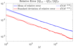
To test the performance of the algorithm, we generate batches of trajectories, where each batch consists of trajectories. For each batch, we divide the trajectories into groups of size , for , where each larger group contains all the trajectories of a smaller group. For each such group of trajectories, we solve the IOC problem (with set to ), and this procedure is repeated for all the batches. This means that we obtain estimates , for and . For each value of , the relative error is averaged over the batches, and the resulting empirical mean and empirical standard deviation (as a function of ) is shown in Figure 1. From the figure we see that, in line with the statistical consistency proved in Theorem 5.4, both the mean and the standard deviation decreases with increasing . Moreover, in Figure 1 the logarithm of the mean and the logarithm of the standard deviation appears to be (approximately) affine in . The figure also shows the corresponding lines obtained by fitting an affine model to each of the two sets of logarithmic data. From this fit, we see that and . We hence suspect that the convergence rate is , and that is asymptotically normal, just like most M-estimators such as maximum log-likelihood [van1998asymptotic, p. 51]. However, a theoretical analysis of this is left for future work.
7 Conclusion
In this work, we have considered the inverse optimal control problem for discrete-time finite-horizon general indefinite linear-quadratic problems with stochastic planning horizons. We first investigate the necessary and sufficient conditions for the when the forward problem is solvable. The identifiability of the corresponding inverse optimal control problem is analyzed and proved. Furthermore, based on the underlying necessary and sufficient condition, we construct the estimator of the inverse optimal control problem as the solution to a convex optimization problem, and prove that the estimator is statistically consistent. The performance of the estimator is illustrated on a numerical example of identifying the evaders cost in non-zero sum pursuit-evasion game.
Appendix A Deferred proofs
Proof of Proposition 2.4..
We show the contraposition of the statement, i.e., that if is such that there exists an initial value and a time-horizon length so that the optimal control problem (1) is unbounded from below, then there exists an initial value so that (1) is unbounded from below for planning horizon length . To this end, consider planning horizon . By Theorem 3.1, if then there exists an such that (4d) or (4e) does not hold for . Splitting the summation in the objective function as
and following along the lines of the proof of “1)2)” in Theorem 3.1, similar to (15) we get the following inequality
Moreover, from the same proof we know that we can select in order to make the terms outside of the last summation unbounded from below. Now, by invertability of , we can select and for . For any value of , this gives an initial condition and a sequence of states and controls that fulfill the constraints (1b)-(1e) (note that (1c) and (1e) are vacuous since ). Moreover it is easily seen that is bounded from above by an expression similar to the one in the previous proof, but containing and additional constant . Following a logic similar to the reminder of the proof of “1)2)” in Theorem 3.1, the result follows. ∎
Proof of Lemma 4.2..
Let be such that . The matrix is symmetric. Let be an orthonormal eigen-decomposition of the matrix. This means that we can write for some real-valued random variables , .
Assume that is not (strictly) positive definite. Then at least one eigenvalue is zero; without loss of generality, let . Then we have that
and thus that . By Jensen’s inequality [bauschke2017convex, Prop. 9.24], we know that , and by following the proof of [bauschke2017convex, Prop. 9.24], we see that equality holds if and only if is constant a.s. (otherwise, the inequality from [bauschke2017convex, Thm. 9.23] is strict at some points). To this end, let a.s. for some constant . If , then for , Assumption 2.5 does not hold. If , then the probability mass of is located on a hyperplane defined by , which does not pass through the origin. In this case, let and note that for we have that for all , hence violating Assumption 2.5. Therefore, we must have . ∎
Proof of Lemma 4.3..
Note that
Hence by Lemma 4.2 and [horn2005basic, Thm. 1.12], we know that for all such that , . On the other hand, by Assumption 2.2, is independent of the noiseless , for , and for such it thus hold that
where . In particular, note that
| (35) |
since is invertible for all and since positive definiteness is invariant under congruence. By induction, we thus have for all such that , and in particular thus for by Assumption 2.3.
Now we show . First, note that . By Assumption 2.5 we have , and hence . In addition, by taking trace on both sides of (35), moving the trace inside the expectation, rearranging terms, and using Cauchy-Schwartz inequality, we have that
Using an induction argument similar to the one above, we thus have that for all and all such that . Finally,
which proves the lemma. ∎