Context Label Learning: Improving Background Class Representations in Semantic Segmentation

Abstract

Background samples provide key contextual information for segmenting regions of interest (ROIs). However, they always cover a diverse set of structures, causing difficulties for the segmentation model to learn good decision boundaries with high sensitivity and precision. The issue concerns the highly heterogeneous nature of the background class, resulting in multi-modal distributions. Empirically, we find that neural networks trained with heterogeneous background struggle to map the corresponding contextual samples to compact clusters in feature space. As a result, the distribution over background logit activations may shift across the decision boundary, leading to systematic over-segmentation across different datasets and tasks. In this study, we propose context label learning (CoLab) to improve the context representations by decomposing the background class into several subclasses. Specifically, we train an auxiliary network as a task generator, along with the primary segmentation model, to automatically generate context labels that positively affect the ROI segmentation accuracy. Extensive experiments are conducted on several challenging segmentation tasks and datasets. The results demonstrate that CoLab can guide the segmentation model to map the logits of background samples away from the decision boundary, resulting in significantly improved segmentation accuracy. Code is available.

I Introduction

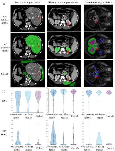
Figure 1: (a) Examples of ROI classes (in red color) along with human-defined context labels and context labels generated automatically by the proposed context label learning (CoLab) in background. Here, human-defined context labels (e.g., liver, kidney, brain tissue) provide additional anatomical information to benefit representation learning. In a similar manner, CoLab automatically finds and labels task-related tissues/structures in background to benefit corresponding ROI segmentation, see Fig. LABEL:fig_contexttask for more details. (b) Self-supervised context labels generated by CoLab can significantly improve the segmentation of different structures with improved Dice similarity coefficient (DSC) and reduced 95% Hausdorff distance (HD), compared to the one trained w/o context labels. The performance gains are comparable and sometimes even higher than the ones using human-defined context labels.

Convolutional neural networks (CNNs) are state-of-the-art approach for semantic image segmentation. Their large number of trainable parameters make them capable to fit to different kinds of tasks yielding high performance in terms segmentation accuracy [zhang2021understanding]. Yet, in real world applications, CNNs seem sometimes unable to capture and generalize from complex, heterogeneous training sets when the amount of training data is limited [novak2018sensitivity]. Specifically, in the case of medical image segmentation, samples from the background class, which provide essential contextual information for regions of interest (ROIs), make up the majority of the training set while containing diverse sets of structures with heterogeneous characteristics, making it hard for the segmentation model to learned accurate decision boundaries.

When trained with datasets with a highly heterogeneous background class, the segmentation model is prone to underfit these contextual samples and fail to separate the ones which share characteristics similar to the ROI samples. The model then produces false positives (FP), yielding systematic over-segmentation. In this study, we argue that underfitting of the contextual information is a main cause of degraded segmentation performance by affecting precision (calculated as $\frac{\text{TP}}{\text{TP}+\text{FP}}$). We observe that better context representation where the background class is decomposed into several subclasses, for example, using additional anatomy labels, significantly improves the ROI segmentation accuracy. We show some examples of human-defined context labels in Fig. 1(a). In the case of liver tumor segmentation, for example, it is beneficial to also have labels for the liver available in addition to the tumor class. Empirically, we find that when training with human-defined context labels, the segmentation model can yield better performance in terms of Dice similarity coefficient (DSC) and 95% Hausdorff distance (HD), as shown in Fig. 1(b). However, these human-defined context labels are not always available and difficult and time-consuming to obtain. In many applications, only the ROI labels, e.g., tumor class, are available. Here, we propose context label learning (CoLab), which automatically generates context labels to improve the learning of a context representation yielding better ROI segmentation accuracy. As demonstrated in Fig. 1(b), CoLab can bring similar improvements when compared with training with human-defined context labels, without the need for expert knowledge.

The contribution of this study can be summarized as follows: 1) With the observations of six datasets, we conclude that underfitting of the background class consistently degrades the segmentation performance by decreasing precision. 2) We find that better context representations with a decomposition of the background class can improve segmentation performance. 3) We propose CoLab, a flexible and generic method to automatically generate soft context labels. We validate CoLab with extensive experiments and find consistent improvements where the segmentation accuracy is en par and sometimes better compared to the case where human annotated context labels are available.

II Related work

II-A Class imbalance

CoLab is related to the class imbalance problem as background commonly constitutes the majority class in image segmentation. However, methods to combat class imbalance mostly focus explicitly on improving the performance of the minority categories [kang2019decoupling, xiang2020learning, liu2019large]. Most approaches ignore the characteristics of majority background class as it is not contributing much to the common evaluation metrics of sensitivity, precision, and DSC of the ROI classes. CoLab focuses specifically on the representation of the background class and is complementary to methods tackling class imbalance such as loss reweighting strategies [cai2021ace].

Previous studies adopt coarse-to-fine strategies to reduce FP in segmentation tasks with class imbalance [setio2016pulmonary, valindria2018small, zhou2017fixed]. However, ROI samples missed in the coarse stage cannot be recovered with later stages. In contrast, CoLab is trained in an end-to-end manner and can reduce varied kinds of FP.

II-B Multi-task learning

CoLab, which is formulated as multi-label classification, can be seen as a form of multi-task learning (MTL). Current MTL methods train the model with different predefined tasks together with the main task using a shared feature representation [li2019deepvolume, qaiser2021multiple, bragman2019stochastic]. Previous works also attempted to incorporate spatial prior [zhang2021automatic, glocker2012joint] or task prior [zhang2020exploring, zhou2019prior] into model training with some predefined auxiliary tasks and optimization functions. In contrast, CoLab reformulates the main task by decomposing the background class with context labels and automatically generate the auxiliary task in a self-supervised manner. We argue that CoLab can have a direct impact on the main task by extending the label space.

The main methodology of the CoLab strategy is inspired by some recently proposed methods which aim to generate the weights for pre-defined auxiliary tasks or labels through a similar meta-learning framework [navon2020auxiliary, liu2019self]. In this study, CoLab is specifically designed for semantic segmentation with heterogeneous background classes which is a common scenario in medical imaging.

III Context labels in image segmentation

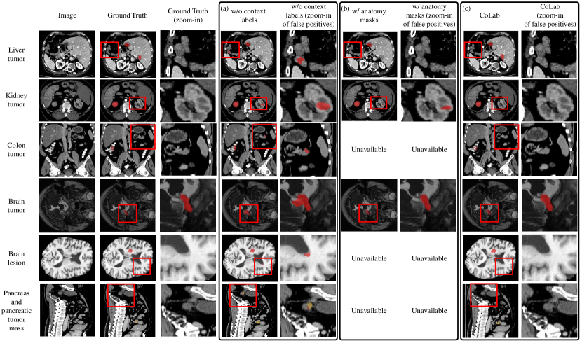
Figure 2: Visualization of different datasets and segmentation results on test data when training w/o and w/ different types of context labels. (a) Models trained without any context labels are prone to over-segmentation of the ROI (red/red + orange) with different kinds of FP (marked with red boxes). (b) Empirically, we observe that adding human-defined context labels such as anatomy masks for supervision helps reduce FP and therefore obtains higher overall segmentation accuracy. (c) The proposed CoLab achieves a similar benefit without requiring additional human annotation by producing context labels automatically.

III-A Preliminaries

We consider CNNs for multi-class segmentation with a total of $c$ classes. Given a training dataset $\mathcal{D}=\{(\boldsymbol{x}_{i},\boldsymbol{y}_{i})\}_{i=1}^{N}$ with $N$ samples, where $\boldsymbol{y}_{i}\in\rm I\!R^{c}$ is the one-hot encoded label for the central pixel in the image sample $\boldsymbol{x}_{i}\in\rm I\!R^{d}$, such that $\boldsymbol{1}\cdot\boldsymbol{y}_{i}=1$ $\forall$ $i$. A segmentation model $f_{\phi}(\cdot)$ learns class representations of the input sample $\boldsymbol{x}_{i}$, noted as $\boldsymbol{z}_{i}=f_{\phi}(\boldsymbol{x}_{i})\in\rm I\!R^{c}$. We obtain the predicted probability $\boldsymbol{p}_{i}$ that the real class of $\boldsymbol{x}_{i}$ is $j$ via a softmax function with $p_{ij}=\mathrm{e}^{z_{ij}}/\sum_{j=1}^{c}\mathrm{e}^{z_{ij}}$. Typically the model is optimized by minimizing the empirical risk $R_{\mathcal{L}_{seg}}(f_{\phi})=\frac{1}{N}\sum_{i=1}^{N}\mathcal{L}_{seg}(f_{\phi}(\boldsymbol{x}_{i}),\boldsymbol{y}_{i})$ computed on the training set. The segmentation loss $\mathcal{L}_{seg}$ can be defined as the sum of losses $\mathcal{L}$ over $c$ classes:

$$\begin{split}&\mathcal{L}_{seg}(f_{\phi}(\boldsymbol{x}_{i}),\boldsymbol{y}_{i})=\sum_{j=1}^{c}\mathcal{L}(p_{ij},y_{ij})\\ &=\underbrace{\sum_{j=1}^{c-1}\mathcal{L}(p_{ij},y_{ij})}_{\text{ROI classes}}+\underbrace{\mathcal{L}(p_{ic},y_{ic})}_{\text{background class}},\end{split}$$ (1)

where $\mathcal{L}$ is a criterion for a specific class, such as cross entropy (CE) or soft DSC [milletari2016v]. Here, we further decompose $\mathcal{L}_{seg}$ into two terms, including an ROI loss (computed on $c-1$ foreground classes) and a background loss (computed on the background class, only).

We aim to improve segmentation performance by augmenting the background class with auxiliary context classes. Specifically, we propose to utilize context labels assigned to different and decomposed background regions. In order to divide the background class into $t>1$ classes, we create another model $\tilde{f}_{\theta}(\cdot)$ with $\tilde{\boldsymbol{z}}_{i}=\tilde{f}_{\theta}(\boldsymbol{x}_{i})\in\rm I\!R^{c+t-1}$ and predicted probability $\tilde{\boldsymbol{p}}_{i}$. We also require an additional one-hot label $\tilde{\boldsymbol{y}}_{i}\in\rm I\!R^{c+t-1}$, where we require $\tilde{y}_{ij}=y_{ij}$ $\forall$ $i$, $j\in\{1,\cdots,c-1\}$ and $\sum_{j=c}^{c+t-1}\tilde{y}_{ij}=y_{ic}$ $\forall$ $i$. With this notion, the segmentation loss can be written as:

$$\begin{split}&\mathcal{L}_{seg}(\tilde{f}_{\theta}(\boldsymbol{x}_{i}),\tilde{\boldsymbol{y}}_{i})=\sum_{j=1}^{c+t-1}\mathcal{L}(\tilde{p}_{ij},\tilde{y}_{ij})\\ &=\underbrace{\sum_{j=1}^{c-1}\mathcal{L}(\tilde{p}_{ij},\tilde{y}_{ij})}_{\text{ROI classes}}+\underbrace{\sum_{j=c}^{c+t-1}\mathcal{L}(\tilde{p}_{ij},\tilde{y}_{ij})}_{\text{background classes}},\end{split}$$ (2)

In the following method section, we always consider a simplified but common case where we only have one ROI class ($c=2$) for simplicity. In other words, we only consider binary ROI segmentation with $f_{\phi}(\boldsymbol{x}_{i})\in\rm I\!R^{2}$, although the method can be naturally extended to multi-class ROI segmentation. With this assumption, Eq. 2 can be simplified as:

$$\mathcal{L}_{seg}(\tilde{f}_{\theta}(\boldsymbol{x}_{i}),\tilde{\boldsymbol{y}}_{i})=\underbrace{\mathcal{L}(\tilde{p}_{i1},\tilde{y}_{i1})}_{\text{ROI class}}+\underbrace{\sum_{j=2}^{t+1}\mathcal{L}(\tilde{p}_{ij},\tilde{y}_{ij})}_{\text{background classes}}$$ (3)

III-B False positives on background class

To better understand the effect of the background class on the model learning, we train multiple CNNs on segmentation datasets which contain heterogeneous background. We conduct experiments on challenging tasks including liver tumor segmentation in computed tomography (CT) images [bilic2019liver], kidney tumor segmentation in CT images [heller2019kits19], colon tumor segmentation in CT images [simpson2019large], vestibular schwannoma (VS) segmentation in T2-weighted magnetic resonance (MR) images [shapey2019artificial], brain stroke lesion segmentation in T1-weighted MR images [liew2018large] and pancreatic tumor segmentation in CT images [simpson2019large]. We adopt a well-configured 3D U-Net [isensee2021nnu] as the segmentation model for all the experiments, which has been demonstrated to yield competitive results across different medical image segmentation tasks. The detailed data and network configurations are summarized in Section V.

Visualizations of the segmentation results are shown in Fig. 2(a). When trained with binary segmentation tasks and without context labels, the models are prone to over-segment the ROIs with many FP. Specifically, the model trained on the binary liver tumor task predicts other organs outside liver as liver tumor; the model trained on the binary kidney tumor task predicts parts of the healthy kidney regions as kidney tumor; while the model trained on the binary brain tumor task predicts the surrounding brain tissue as brain tumor; the model trained on the binary brain lesion task predicts unrelated healthy brain regions as brain lesion.

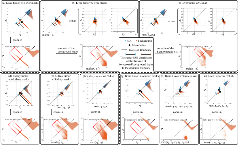
Figure 3: The distribution of activations (logits) after the classification layer using ROI (blue) or background samples (orange) of test data as network input. Here, $z_{1}$ denotes logits for ROI classes, while $z_{i}\;(i>1)$ denotes logits for background classes. We also report the number of pixel-level predictions that are FP. Without context labels (a, d, g), CNNs fail to map the background samples to compact clusters. This is because CNNs are forced to learn generic filters for the background samples, yielding similar activations regardless of different background structures with diverse patterns/appearance. Consequently, the logit distribution of background samples would spread across the decision boundary, leading to increased FP. Extending the label space with anatomy masks (b, e, h) or CoLab (c, f, i) can alleviate this issue.

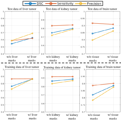
Figure 4: Performance on liver tumor, kidney tumor and brain tumor segmentation on training data (lower part) and testing data (upper part) when networks were trained w/o and w/ context labels. Extending the label space with anatomy masks can help the model improve the performance by increasing the precision, while the sensitivity is largely retained.

III-C Underfitting of background samples

To study the model behavior when trained with heterogeneous background classes, we can monitor the logit distribution of samples from ROI and background classes for the test data. Our observations for liver tumor, kidney tumor, and brain tumor segmentation are summarized in Fig. 3(a, d, g).

We find that the CNN models map the ROI samples to a compact cluster in the logit space while background samples form a more dispersed distribution. This indicates that the model cannot easily map all background samples to a single cluster representing the background class. Although the model seems to separate ROI from background samples in the feature space, it builds complex background representations and unable to capture an accurate decision boundary between ROI and immediate context. A possible reason is that the CNN uses most of its capacity to extracted the common features among background regions with different characteristics. Unfortunately, these shared features are not very discriminate. Specifically, we observe that the logit distribution of background samples overlaps with the learned decision boundary. This is the reason why the model predicts many FP leading to over-segmentation of ROI structures when the background class is heterogeneous. We hypothesise that the width of the distribution serves as an indicator of the heterogeneity of a specific class and is a sign of the difficulty during learning. As a result of sample heterogeneity, a CNN may struggle to reduce intra-class variation of the background class and underfit the background samples, failing to recognize the background samples that share similar characteristics with ROI samples.

It should be noted that we do not observe significant difference between the logit distribution of training background samples and test background samples, as also shown in previous studies [li2019overfitting, li2020analyzing], indicating that the logit shift of background samples is indeed due to underfitting instead of overfitting.

III-D The effect of context labels

The availability of context labels greatly helps with the ROI segmentation, which provide additional signals to CNN to fit the training data of heterogeneous background samples. We confirm this empirically by including human-defined context labels in the model training. Specifically, we adopt liver masks ($t=2$) for liver tumor segmentation, kidney masks ($t=2$) for kidney tumor segmentation, brain tissue masks including ventricles, deep grey matter, cortical grey matter, white matter and other tissues ($t=6$) for brain tumor segmentation. The kidney and liver masks are manually annotated, while the brain tissue masks are generated automatically using the paired T1-weighted MR images and a multi-atlas label propagation with expectation–maximisation based refinement (MALP-EM) [ledig2015robust]. In order to make a fair comparison, we make sure that all the experiments share the same training schedule except the label space. We sample the training patches only considering ROIs. Specifically, we make sure 50% training patches to contain ROIs and sample the other half of the training patches uniformly.

The observations on test and training set are summarized in Fig. 4. We find that the models yield overall better performance when trained with anatomy masks, as indicated by improved DSC (defined as $DSC=2\frac{\text{sensitivity}\cdot\text{precision}}{\text{sensitivity}+\text{precision}}$). Furthermore, we observe that the model trained with context labels yields higher precision while preserving similar sensitivity. The observation is consistent with the visualization results in Fig. 2(b), where we find the models trained with human-defined context labels reduce FP.

Similarly, we visualize the corresponding network behaviour in Fig. 3(b, e, h). As we only consider the segmentation performance of the ROI (class 1), we visualize the logits in the plane of ($z_{1}$, max($z_{2}$, …, $z_{t+1}$)). We observe that the model trained with anatomy masks maps the background samples to a narrower distribution and reduces the background logits shift across the decision boundary. This indicates that the models fit the training data better with the help of context labels. Instead of building generic filters for all the background samples, the CNNs can dedicate specific filters to model a more homogeneous subparts of the background samples that share common characteristics. The models are faced with a simplified segmentation task with homogeneous background subclasses yielding better overall performance with the same model capacity.

Although anatomy masks are found to be effective context labels, they are not always available in real-world applications. Specifically acquiring manually annotated context labels is time-consuming and would require significant efforts from human experts to generate annotations at large scale. Therefore, we propose CoLab which can automatically discover specific soft context labels using a meta-learning strategy. CoLab benefits the segmentation model training by making it to fit the background samples better, achieving comparable or even better performance when compared with models trained on manually defined anatomy masks.

IV CoLab

IV-A Overview

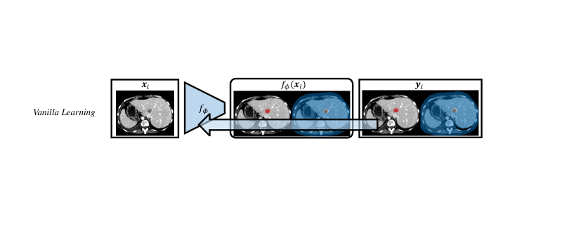
Figure 5: Illustration of the training process of CoLab. $g_{\omega}(\cdot)$ is optimized to generate context labels such that it can help reduce the training loss of the ROI in the most effective way, see Section IV-A for more details.

Now we consider CNNs for binary semantic segmentation. Typically, we are given a baseline segmentation model $f_{\phi}(\cdot)$ that maps the input image $\boldsymbol{x}_{i}$ to the label space $f_{\phi}(\boldsymbol{x}_{i})\in\rm I\!R^{2}$. In order to fit the label space with context labels, we first extend the classification layer of $f_{\phi}(\cdot)$ with additional $t-1$ output neurons and obtain $\tilde{f}_{\theta}(\cdot)$ which map $\boldsymbol{x}_{i}$ to $\tilde{f}_{\theta}(\boldsymbol{x}_{i})\in\rm I\!R^{t+1}$. We employ another model $g_{\omega}(\cdot)$ as the task generator parameterized by $\omega$ to produce context labels, with the network output $\boldsymbol{o}_{i}$ = $g_{\omega}(\boldsymbol{x}_{i})\in\rm I\!R^{t}$. We have no requirements for the backbone of $g_{\omega}(\cdot)$ and empirically keep it the same with that of $f_{\phi}(\cdot)$.

We illustrate the training process of the proposed CoLab in Fig. 5. At the beginning of each iteration, we obtain the context labels termed as distance constrained label $\hat{\tilde{\boldsymbol{y}}}_{i}$ by taking use of $\boldsymbol{o}_{i}$ and the ground truth $\boldsymbol{y}$. This process is marked with ① and will be illustrated in Section IV-B and IV-C. Then, we calculate a new $\theta^{*}$ with one step of gradient descent with ② to access the impact of $\hat{\tilde{\boldsymbol{y}}}_{i}$ on model training of ROI segmentation. Next, we optimize $\omega$ based on the second-order derivatives through a meta learning scheme with ③, which would be demonstrated in Section IV-D. Finally, we optimize the segmentation model $\tilde{f}_{\theta}(\cdot)$ based on the updated context labels with ④.

IV-B Label aggregation

We calculate the context probability $(q_{ij})_{j=1}^{t}$ based on $\boldsymbol{o}_{i}$ via the softmax function as:

$$q_{ij}=\frac{\mathrm{e}^{o_{ij}}}{\sum_{j=1}^{t}\mathrm{e}^{o_{ij}}}.$$ (4)

The extended label $\tilde{\boldsymbol{y}}_{i}\in\rm I\!R^{t+1}$ is calculated by aggregating the original label $\boldsymbol{y}_{i}=(y_{i1},y_{i2})$ and the context probability $\boldsymbol{q}_{i}$ with:

$$\tilde{y}_{ij}=\left\{\begin{array}[]{rcl}y_{i1}&&\text{if}\quad j=1,\\ q_{ij}&&\text{if}\quad j>1\quad\text{and}\quad y_{i1}=0,\\ 0&&\text{otherwise.}\end{array}\right.$$ (5)

The label aggregation process is also illustrated in Fig. 6. By doing so, we can decompose the background class $y_{i2}$ into $t$ subclasses while ensure that the $\tilde{\boldsymbol{y}}_{i}$ contains sufficient information about the ROI segmentation. For multi-class segmentation with totally $c$ classes, $\tilde{\boldsymbol{y}}_{i}$ can be calculated as:

$$\tilde{y}_{ij}=\left\{\begin{array}[]{rcl}y_{ij}&&\text{if}\quad j<c,\\ q_{ij}&&\text{if}\quad j\geq c\quad\text{and}\quad y_{ij}=0\quad\forall j<c,\\ 0&&\text{otherwise.}\end{array}\right.$$ (6)

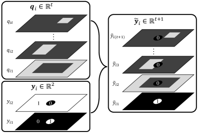
Figure 6: Illustration of the label aggregation process. We generate the extended label $\tilde{\boldsymbol{y}}_{i}$ by aggregating the original label $\boldsymbol{y}_{i}$ with the context probability $\boldsymbol{q}_{i}$.

IV-C Context constraints

Compared with background samples which are further away, the ones closer to the ROIs share similar characteristics with ROI samples and are more likely to be misclassified. In order to make the segmentation model focus more on those hard background samples that are close to ROIs, we make an assumption that all samples which are distant from the ROI need less attention and should be safely assigned the same background label. Specifically, we create a hard label $\boldsymbol{b}_{i}\in\rm I\!R^{t+1}$ to represent the the background samples that are far from the ROI:

$$b_{ij}=\left\{\begin{array}[]{rcl}1&&\text{if}\quad j=2,\\ 0&&\text{otherwise}.\end{array}\right.$$ (7)

By utilizing the ROI label $\boldsymbol{y}_{i}$, we calculate the corresponding distance map $d_{i}$ which is the Euclidean distance of a pixel to the closest boundary point of the ROI of any class. We set $d_{i}$ to be zero for pixels inside the ROI.

We then calculate a soft dilated mask $\mathcal{M}_{i}$ based on $d_{i}$:

$$\mathcal{M}_{i}=\left\{\begin{array}[]{rcl}1&&\text{if}\quad d_{i}<m,\\ \mathrm{e}^{\frac{-d_{i}+m}{\tau}}&&\text{otherwise,}\end{array}\right.$$ (8)

where $m$ is the margin controlling the model’s focus on the pixels which are neighbouring to ROI and $\tau$ is the temperature to control the probabilities of the dilated regions. Empirically, $m$ is set as 30 and $\tau$ is set as 20 for all our experiments. $\mathcal{M}_{i}$ would be 1 for pixels around ROIs and decrease close to 0 for pixels far from ROIs. We visualize an example of $\mathcal{M}_{i}$ with liver tumor in Fig. 7. The distance constrained label then is calculated as:

$$\hat{\tilde{\boldsymbol{y}}}_{i}=\mathcal{M}_{i}\tilde{\boldsymbol{y}}_{i}+(1-\mathcal{M}_{i})\boldsymbol{b}_{i}.$$ (9)

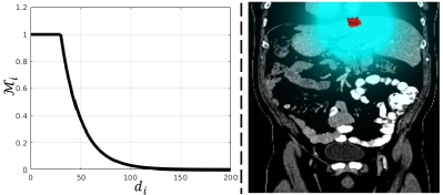
Figure 7: The task generator focuses on the context which is near to the ROI. To do so, we train the segmentation model to classify the pixels which are outside the soft dilated ROI as the same class (pixels marked without color in the right figure). (Left part) The value of a soft dilated mask $\mathcal{M}_{i}$ with $m=30$ and $\tau=20$. (Right part) The visualization of the dilated mask $\mathcal{M}_{i}$ (blue) with a liver tumor (red) of a training case.

In this way, only the regions neighbouring to the tumor are considered to be classified as the contextual background class. Specifically, both $\tilde{f}_{\theta}(\cdot)$ and $g_{\omega}(\cdot)$ would be trained to focus on the regions which are close to ROIs.

IV-D Task generator optimization with meta-gradients

We formulate the optimization of CoLab as a bi-level problem:

$$\min_{\omega}\frac{1}{N}\sum_{i=1}^{N}\mathcal{L}_{ROI}(\tilde{f}_{\theta^{*}}(\boldsymbol{x}_{i}),\boldsymbol{y}_{i})$$ (10)

$$s.t.\quad\theta^{*}=\operatorname*{argmin}_{\theta}\frac{1}{N}\sum_{i=1}^{N}\mathcal{L}_{seg}(\tilde{f}_{\theta}(\boldsymbol{x}_{i}),\hat{\tilde{\boldsymbol{y}}}_{i})),$$ (11)

where $\mathcal{L}_{ROI}(\tilde{f}_{\theta}(\boldsymbol{x}_{i}),\boldsymbol{y}_{i})=\mathcal{L}_{c}(\tilde{p}_{i1},y_{i1})$ is computed on the ROI class. Different from $\mathcal{L}$, we choose $\mathcal{L}_{c}$ to be a criteria that can be calculated in the one-versus-all manner, such as binary cross entropy (BCE) and soft DSC loss, to represent the binary segmentation performance of the ROI class with more than two output logits.

We train the model using a batch of training samples with batch size $n$. For simplicity, we shorten $\frac{1}{n}\sum_{i=1}^{n}\mathcal{L}_{ROI}(\tilde{f}_{\theta^{*}}(\boldsymbol{x}_{i}),\boldsymbol{y}_{i})$ as $\mathcal{L}_{ROI}(\theta^{*})$ and $\frac{1}{n}\sum_{i=1}^{n}\mathcal{L}_{seg}(\tilde{f}_{\theta}(\boldsymbol{x}_{i}),\hat{\tilde{\boldsymbol{y}}}_{i})$ as $\mathcal{L}_{seg}(\theta,\omega)$ in the following descriptions. The bi-level optimization problem defined in Eq. 10 and 11 can be solved with gradient descent [pedregosa2016hyperparameter, franceschi2018bilevel]. Specifically, the derivative of $\mathcal{L}_{ROI}(\theta^{*})$ w.r.t. $\omega$ can be calculated by applying the chain rule:

$$\nabla_{\omega}\mathcal{L}_{ROI}(\theta^{*})=(\frac{\partial\theta^{*}}{\partial\omega})^{\intercal}\nabla_{\theta}\mathcal{L}_{ROI}(\theta^{*}),$$ (12)

where $\nabla_{\omega}=(\frac{\partial}{\partial\omega})^{\intercal}$ and $\nabla_{\theta}=(\frac{\partial}{\partial\theta})^{\intercal}$. One can compute $\frac{\partial\theta^{*}}{\partial\omega}$ based on implicit function theorem [bengio2000gradient]. However, the derived result would contain a Hessian which is computational expensive and not always possible to access for deep neural networks. Among the many heuristics for the gradient approximation [pedregosa2016hyperparameter, franceschi2018bilevel, liu2018darts], we follow the solution described in [finn2017model, liu2018darts] to approximate $\theta^{*}$ by a single optimization step. Specifically, we sample a batch of training data and approximate the optimal inner variable $\theta^{*}$ with a step of gradient decent:

$$\theta^{*}\approx\theta-\alpha\nabla_{\theta}\mathcal{L}_{seg}(\theta,\omega),$$ (13)

where $\alpha$ is step size, which is kept the same with the learning rate of $\theta$. We differentiate this equation w.r.t. $\omega$ from both sides yielding:

$$\frac{\partial\theta^{*}}{\partial\omega}=-\alpha\nabla^{2}_{\theta,\omega}\mathcal{L}_{seg}(\theta^{*},\omega),$$ (14)

where $\nabla^{2}_{\theta,\omega}=\frac{\partial\nabla_{\theta}}{\partial\omega}$. By substituting Eq. 14 into Eq. 12, we can obtain the gradient on $\omega$ and update it with:

$$\omega^{t+1}=\omega^{t}-\beta\nabla_{\omega^{t}}\mathcal{L}_{ROI}(\theta^{*})$$ (15)

$$=\omega^{t}+\alpha\beta\nabla^{2}_{\omega^{t},\theta}\mathcal{L}_{seg}(\theta^{*},\omega^{t})\nabla_{\theta}\mathcal{L}_{ROI}(\theta^{*}),$$

where $\beta$ is the learning rate to update $\omega$. In this way, the task generator $g_{\omega}$ is explicitly trained to produce effective context labels with the second-order gradients. Although Eq. 15 contains an expensive vector-matrix product, it is feasible to calculate with prevailing machine learning frameworks such as PyTorch [paszke2019pytorch]. We find CoLab can be efficient as it costs as little as 30% additional training time. We summarize the implementation details in supplementary material. The full algorithm is summarized in Algorithm 1.

Algorithm 1 Context label learning (CoLab)

1:

2:$\mathcal{D}=\{(\boldsymbol{x}_{i},\boldsymbol{y}_{i})\}_{i=1}^{N}$: training data; $t$: the number of context classes, $f_{\phi}(\cdot)$: the segmentation model which produces $f_{\phi}(\boldsymbol{x}_{i})\in\rm I\!R^{2}$; $g_{\omega}(\cdot)$: the task generator which produce $g_{\omega}(\boldsymbol{x}_{i})\in\rm I\!R^{t}$.

3:$\alpha$, $\beta$: learning rates to update $\theta$ and $\omega$.

4:Extend the classification layer of $f_{\phi}(\cdot)$ to get $\tilde{f}_{\theta}(\cdot)$ which produce $\tilde{f}_{\theta}(\boldsymbol{x}_{i})\in\rm I\!R^{t+1}$.

5:for each iteration do

6:     Sample a batch of data $\mathcal{B}=\{(\boldsymbol{x}_{i},\boldsymbol{y}_{i})\}_{i=1}^{n}$ from $\mathcal{D}$.

7:     for a number of steps do $\triangleright$ Note: One step is sufficient in our experiments.

8:         Generate the context probability $\boldsymbol{q}_{i}$ based on the output of task generator $g_{\omega}(\boldsymbol{x}_{i})$ via Eq. 4.

9:         Generate the extended label $\tilde{\boldsymbol{y}}_{i}$ by aggregating the context probability $\boldsymbol{q}_{i}$ with $\boldsymbol{y}_{i}$ via Eq. 5.

10:         Calculate a loss mask $\mathcal{M}_{i}$ via Eq. 8 and generate the distance constrained label $\hat{\tilde{\boldsymbol{y}}}_{i}$ via Eq. 9.

11:         Calculate a new $\theta^{*}$ with the gradient descent optimization algorithm via Eq. 13.

12:         Optimize $\omega$ based on meta-gradients via Eq. 15. $\triangleright$ Training the task generator.

13:     end for

14:     Update $\theta$ with gradient decent based on updated $\omega$. $\triangleright$ Training the segmentation model.

15:end for

V Experiments

V-A Experimental setup

V-A1 Network configurations

We use a state-of-the-art 3D U-Net [isensee2021nnu] as the network backbone for both the segmentation model $f_{\phi}$/$\tilde{f}_{\theta}$ and the task generator $g_{\omega}$. We normalize all datasets with the built-in pipeline following [isensee2021nnu]. Specifically, we adopt case-wise Z-score normalization within brain masks for MR images, while we employ dataset-wise Z-score normalization based on ROI samples for CT images after clipping the Hounsfield units (HU) from 0.5% to 99.5%. We utilize the default data augmentation policies for all experiments. We adopt a combination of CE and sample-wise soft DSC loss with equal weight for $\mathcal{L}$ while using BCE for $\mathcal{L}_{c}$. We use a batch size of 2 and patch size of 80$\times$80$\times$80. We train the networks for 1000 epochs for brain tumor and lesion segmentation and 2000 epochs for liver, kidney, colon and pancreas tumor segmentation as we observed that the network needed more iterations to converge latter tasks. We summarize the hyper-parameters of all experiments in supplementary material. All reported results are the average of two runs with different random seeds.

V-A2 Liver tumor segmentation

We evaluate CoLab for liver tumor segmentation with the training dataset from the Liver Tumor Segmentation Challenge (LiTS) which contains 131 CT images. We exclude the samples which do not contain any liver tumor leaving 118 cases. We resample all CT images to a common voxel spacing of 1.9$\times$1.9$\times$2.5 mm following [isensee2021nnu]. We train models with 83 cases and test on 35 cases.

V-A3 Kidney tumor segmentation

We further conduct experiments using the training dataset of the Kidney Tumor Segmentation Challenge (KiTS) which contains 210 CT images. We resample all CT images to a common voxel spacing of 1.6$\times$1.6$\times$3.2 mm following [isensee2021nnu]. We tested on 70 cases and used the other 140 cases as the training data.

V-A4 Colon tumor segmentation

We evaluate CoLab for the case of colon tumor segmentation from CT images. We collect 126 colon cancer CT images from the training dataset of the Medical Segmentation Decathlon challenge [simpson2019large]. We resample all CT images to the voxel spacing of 1.6$\times$1.6$\times$3.1 mm following [isensee2021nnu]. We train models with 88 cases and test on the other 38 cases.

V-A5 Brain tumor segmentation

We also conduct experiments for brain tumor segmentation using the VS dataset [shapey2019artificial] which contains 243 paired T1-weighted and T2-weighted MR images. We only used T2-weighted MR images for evaluating CoLab but used T1-weighted MR images to generate the brain structure masks with MALP-EM. We did not use brain masks for the histogram normalization of this task because VS can appear at the brain boundary and may be excluded when using common brain extraction algorithms. All MR images have the same isotropic voxel spacing of 1.0 mm³. We train the models with 176 cases and test on 46 cases following [shapey2019artificial].

V-A6 Brain stroke lesion segmentation

Additionally, we evaluate CoLab with brain stroke lesion segmentation using the Anatomical Tracings of Lesions After Stroke (ATLAS) dataset [liew2018large] which contains 220 T1-weighted MR images. The MR images all have the same voxel spacing of 1.0 mm³. We randomly selected 145 cases as training data and left the rest 75 cases for testing.

V-A7 Pancreas and pancreatic tumor mass segmentation

We further evaluate Colab in the setting of multi-class segmentation. Specifically, we train the segmentation model to segment three classes including pancreas, pancreatic tumor mass and background. We aim to find the context labels which can benefit the segmentation of both foreground classes. We collect 281 CT images containing pancreas tumor from the training dataset of the Medical Segmentation Decathlon challenge [simpson2019large, attiyeh2018survival, attiyeh2019preoperative, chakraborty2018ct]. We resample all the CT images to the voxel spacing of 1.3$\times$1.3$\times$2.6 mm following [isensee2021nnu]. We randomly split the dataset into 197 cases for training and 84 cases for testing.

V-B Compared methods and processing

V-B1 Context labels based on k-means

We compare CoLab with alternative approaches for context label generation, including a context label generation via clustering. Here, we take pixels inside the body masks or brain masks as samples and employ $k$-means [arthur2006k] to construct $t$ clusters. We kept $t$ the same with the class number of human-defined anatomy masks. Specifically, we chose $t=2$ for liver, kidney, colon and pancreas tumor segmentation and $t=6$ for brain tumor and brain stroke lesion segmentation.

V-B2 Context labels based on dilated masks

We also compare with a baseline using dilated masks of the ROI as the context labels. This idea is somewhat similar to label smoothing [muller2019does, islam2021spatially] where models are trained with blurred ROI labels. Specifically, we take the soft dilated masks $\mathcal{M}_{i}$ defined in Eq. 8 and set the context probability as $\boldsymbol{p}_{i}=[1-\mathcal{M}_{i},\mathcal{M}_{i}]^{\intercal}$.

V-B3 Context labels predicted with external datasets

We further evaluate and compare to an approach which leverages prior knowledge from other datasets. Specifically, we trained a segmentation model with 20 CT images using data from [xu2015efficient] which contains labels of 14 abdominal organs including liver and kidney. We resample the 20 CT images to the voxel spacing of 1.6$\times$1.6$\times$3.2 mm. We reduce the dependency of the model on longitudinal axis and trained the segmentation model with a patch size of 128$\times$128$\times$32 as the slice numbers differ across datasets. We then apply this segmentation model to the resampled training split of LiTS as well as KiTS, and extract the liver and kidney masks as the automatically generated contextual anatomy masks.

V-B4 Post-processing

We also compare with a common strategy to suppress FP in segmentation based on component-based post-processing, which is widely adopted in many segmentation pipelines [isensee2021nnu]. Specifically, we assume there is always one ROI and remove all but the largest region. For the cases when ROIs contain multiple classes (pancreas and pancreatic tumor segmentation), we take all the ROIs as a whole and only keep the largest component.

V-C Quantitative results

TABLE I: Evaluation of different binary segmentation tasks with different types of context label generation approaches. We divide the results according to whether expert knowledge and labeling efforts are included. The best and second best results without human efforts are in bold with the best also underlined.

3 Task Method $t$ DSC SEN PRC HD 1 Liver tumor [bilic2019liver] w/o liver masks 1 54.4 58.8 58.9 111.1 $K$-means [arthur2006k] 2 61.4 61.4 67.0 71.9 Dilated masks [muller2019does] 2 60.7 59.8 68.0 67.6 CoLab 2 62.5 62.8 67.3 69.4 CoLab 4 57.3 60.5 62.3 56.3 CoLab 6 59.7 60.3 65.2 43.6 w/ model-predicted liver masks [xu2015efficient] 2 62.4 61.6 70.6 44.1 w/ liver masks [bilic2019liver] 2 62.8 62.1 69.1 53.5 Kidney tumor [heller2019kits19] w/o kidney masks 1 74.9 83.2 71.9 120.4 $K$-means [arthur2006k] 2 76.8 83.5 74.3 87.1 Dilated masks [muller2019does] 2 76.4 83.9 73.1 95.3 CoLab 2 78.5 82.2 77.7 75.7 CoLab 4 76.4 80.6 76.5 63.7 CoLab 6 74.9 81.0 73.3 79.4 w/ model-predicted kidney masks [xu2015efficient] 2 79.2 81.3 82.7 38.1 w/ kidney masks [heller2019kits19] 2 79.9 84.1 78.9 54.7 Colon tumor [simpson2019large] w/o context labels 1 45.6 53.9 45.3 154.9 $K$-means [arthur2006k] 2 44.9 47.2 48.7 111.7 Dilated masks [muller2019does] 2 47.1 49.8 52.8 83.3 CoLab 2 48.9 53.9 50.3 86.0 CoLab 4 45.3 48.1 51.5 81.2 CoLab 6 46.1 50.2 49.7 88.9 Brain tumor [shapey2019artificial] w/o tissue masks 1 84.3 91.2 80.5 15.2 $K$-means [arthur2006k] 6 85.0 91.3 80.3 9.4 Dilated masks [muller2019does] 2 84.8 91.6 81.1 8.8 CoLab 2 85.2 90.4 82.5 7.8 CoLab 4 89.0 91.7 86.7 1.4 CoLab 6 87.9 92.0 84.9 2.5 w/ tissue masks [shapey2019artificial, ledig2015robust] 6 88.2 90.9 86.2 3.1 Brain lesion [liew2018large] w/o context labels 1 58.5 68.2 58.6 51.7 $K$-means [arthur2006k] 6 60.0 60.7 70.5 19.5 Dilated masks [muller2019does] 2 61.9 69.8 63.3 35.3 CoLab 2 62.8 68.2 67.4 28.1 CoLab 4 62.6 68.1 65.4 25.1 CoLab 6 61.7 66.7 65.7 24.5

TABLE II: Evaluation of pancreas and pancreatic tumor mass segmentation with different types of context label generation approaches. The best and second best results are in bold with the best also underlined.