Metaphorical Polysemy Detection:
Conventional Metaphor meets Word Sense Disambiguation

Abstract

Linguists distinguish between novel and conventional metaphor, a distinction which the metaphor detection task in NLP does not take into account. Instead, metaphoricity is formulated as a property of a token in a sentence, regardless of metaphor type. In this paper, we investigate the limitations of treating conventional metaphors in this way, and advocate for an alternative which we name metaphorical polysemy detection (MPD). In MPD, only conventional metaphoricity is treated, and it is formulated as a property of word senses in a lexicon. We develop the first MPD model, which learns to identify conventional metaphors in the English WordNet. To train it, we present a novel training procedure that combines metaphor detection with word sense disambiguation (WSD). For evaluation, we manually annotate metaphor in two subsets of WordNet. Our model significantly outperforms a strong baseline based on a state-of-the-art metaphor detection model, attaining an ROC-AUC score of $.78$ (compared to $.65$) on one of the sets. Additionally, when paired with a WSD model, our approach outperforms a state-of-the-art metaphor detection model at identifying conventional metaphors in text ($.659$ F1 compared to $.626$).

1 Introduction

Linguists differentiate between two types of metaphor: novel and conventional. While novel metaphors are creative expressions made in a particular situation by one particular individual, conventional metaphors are those which have been widely adopted by a language community. Consider:

1. The attack began at dawn.

2. The government has come under attack.

3. The government torpedoed the housing bill.

Example (1) is a literal usage of attack which refers to a military offensive. Example (2) is a conventional metaphor referring to intense verbal criticism. Example (3) is a novel metaphor, which reuses the well-established imagery from (2), but extends it with the word torpedoed.

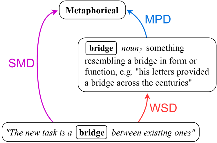
Figure 1: Metaphorical polysemy detection is the missing link between standard metaphor detection and word sense disambiguation

Detecting novel metaphors and conventional metaphors are fundamentally different tasks. Novel metaphors are creative usages of words, which violate statistical patterns of language (e.g. Wilks, 1975, 1978), and which extend the meaning of a word into unexpected areas of semantic space. Conventional metaphors, on the other hand, can be considered lexicalised: examples (1) and (2) come from the gloss of two senses of attack in WordNet (Miller, 1995), where the novel sense of torpedoed in example (3) is not yet captured. Despite these inherent differences, in NLP the standard metaphor detection task, abbreviated as SMD here, makes no distinction between novel and conventional metaphor.

Sense	Definition	Metaphor?
adopt1	take into one’s family (e.g. They adopted two children from Nicaragua)	✗
adopt2	choose and follow; as of theories, ideas, policies, strategies or plans	✓
adopt3	take on a certain form, attribute, or aspect (e.g. he adopted an air of superiority)	✓
adopt4	take up the cause, ideology, practice, method, of someone and use it as one’s own (e.g. They adopted the Jewish faith)	✓

Table 1: Verbal senses of adopted in WordNet

Although recent works have produced resources which distinguish between novel and conventional metaphors (Parde and Nielsen, 2018; Do Dinh et al., 2018), both metaphor types are annotated as properties of tokens, suitable for SMD. In this work, we demonstrate the shortcomings of this formulation, and argue that conventional metaphoricity is best treated not as a property of word occurrences in a sentence, but of word senses in a lexicon. With this in mind, we investigate the problem of assigning metaphoricity ratings to word senses, a problem we name metaphorical polysemy detection (MPD). We build the first model of MPD, which identifies metaphorical senses in WordNet (Miller, 1995).

No training data is available for this task. We design a novel training regime which utilises existing resources, which works by decomposing SMD into two steps: word sense disambiguation (WSD) and MPD (see Figure 1). More specifically, we pair our MPD model with a state-of-the-art WSD model, and train them in conjunction on SMD data, treating word sense as a latent variable.

To investigate the performance of our model, we establish an evaluation framework for MPD. To collect test data, we perform an annotation study, and label two subsets of WordNet for metaphoricity (${\kappa=0.78}$). Metaphor detection is typically evaluated using F1-score, which measures how well a model can judge metaphoricity in absolute terms. For MPD, we additionally introduce a new quantity for evaluation, which we call relative metaphoricity. It measures whether a model is able to correctly identify whether one sense is more metaphorical than another, even if it is unable to correctly determine where they sit around a threshold. It is calculated using ROC-AUC.

On one of our test sets, consisting of words from a large resource of conventional metaphors (the Master Metaphor List; Lakoff et al., 1991), our MPD model attains $.78$ ROC-AUC and $.60$ F1, significantly higher than a strong baseline which uses a state-of-the-art SMD model (MelBERT; Choi et al., 2021), which scores $.65$ and $.54$ respectively. Additionally, for SMD on conventional metaphors, when our model is paired with a WSD model it attains $.659$ F1, significantly better than the state-of-the-art SMD model ($.626$).

2 Metaphor in the Lexicon

A fundamental feature of language is polysemy, the phenomenon of a wordform exhibiting multiple meanings which are systematically related. When meanings are related by metaphorical similarity, the phenomenon is called metaphorical polysemy. An example is the word attack, which describes either a physical confrontation, or—metaphorically—heated criticism (e.g. “she attacked my arguments”). Instances of metaphorical polysemy are called conventional metaphors.

In this section, we describe how conventional metaphors materialise in lexica (§ 2.1). With this in mind, we illustrate the shortcomings of the existing metaphor detection task (§ 2.2), and propose an alternative formulation which is more suitable for conventional metaphors (§ 2.3).

2.1 Metaphoricity of Word Senses

In a lexicon, metaphoricity can be formulated as a property of word senses. Consider the example definitions of the word adopted in WordNet (Miller, 1995), which are shown in Table 1 (some senses are excluded for brevity). Sense adopt₁ is literal, but the other senses are conventional metaphors.

The conventionality of a metaphor lends itself to treatment as a continuous property. For instance, a metaphor used by an entire language community would be highly conventionalised, while a metaphor used by speakers in a particular geographic region would be moderately conventionalised. Novel metaphors sit at the extreme other end of the spectrum: they are creative expressions with ad-hoc meanings. By definition, lexica designed to encode widespread language use will only encode the most conventional of metaphors as word senses.

In order to formulate metaphoricity as a property of word senses, a lexicon needs to encode the literal and metaphorical meanings of a wordform as separate senses. The criteria that need to be met for two meanings to be considered distinct is highly contentious, with some lexicographers arguing that senses should be represented as spectra rather than discrete units (see Cruse, 1986, Ch. 3). In practice, however, lexica describe senses as discrete objects. Moreover, in most lexica the granularity of these senses is high enough to separate metaphorical senses from literal ones, which thus matches our criteria. That being said, no existing lexicon systematically labels senses for metaphoricity (the decision of whether to label metaphorical senses as such is left to the lexicographer’s discretion).

Sentence Excerpt	Prediction
…the South Carolina nullifiers adopted the principle of state interposition…	Metaphorical
…the methods he adopted to accomplish…	Metaphorical
…the denomination’s 16 basic beliefs adopted in 1966…	Metaphorical
…the Government’s new feed grain program was adopted; the program…	Literal
…the Albany Plan of Union, which, had it been adopted, might…	Literal
…the use of target-hunting noses on the projectiles has been adopted, and…	Literal

Table 2: MelBERT makes inconsistent predictions for occurrences of adopted with sense adopt₂ in SemCor

If word senses in a lexicon like WordNet were labeled for metaphoricity, this would be useful in a number of areas of study. When a language community need to reference a newly-arisen meaning, instead of creating a new wordform, often an existing word is extended metaphorically (e.g. a computer mouse). This process of metaphorical extension is a cornerstone of lexical-semantic language change (Koch, 2016), and knowing which word senses were metaphorical would open up new possibilities to study this phenomenon. The metaphors which do enter the lexicon participate in sophisticated patterns, preserving the structure of their literal domains: just as one can attack an opponent in a debate, so too can claims be defended, different rhetorical strategies adopted, and so on. These patterns are known as conceptual metaphors (Lakoff and Johnson, 1980), and knowing which word senses in a lexicon were metaphorical would create new opportunities to analyse their substructures (this has been previously recognised by Lönneker, 2003).

2.2 Issues with Standard Metaphor Detection

In the standard metaphor detection (SMD) task, metaphoricity is formulated as a property of a token in a sentence. The dataset which is almost universally used for this is the VUAMC (Steen et al., 2010). It contains tokenised English sentences, in which words are annotated with binary metaphoricity labels. It was the subject of two recent metaphor detection shared tasks (Leong et al., 2018, 2020).

The VUAMC was annotated following an adapted version of the Metaphor Annotation Procedure (MIP; Crisp et al., 2007). To annotate each token, MIP involves a three-stage process:

1. Establish the contextual meaning of the word, based on the other words in the sentence.

2. Determine whether the word has a more basic meaning which occurs in different contexts (where “basic” meanings are defined as those more concrete, related to bodily action, less vague, and/or historically older).

3. If the word does have a more basic meaning in different contexts, decide whether the meaning in this context can be understood in comparison with the more basic meaning.

If the wordform does have a more basic meaning which the contextual meaning relates to, the token is labeled as a metaphor.

To perform well in SMD, a model must emulate this procedure. There are two drawbacks to this task formulation:

Learning WSD Implicitly

For conventional metaphors, stage 1 of MIP is very similar to word sense disambiguation (WSD). In WSD, the goal is to identify the sense evoked by a wordform in a sentence. This is a hard task in its own right, and, in order to perform well, models of SMD are expected to learn to do this implicitly.

We can check whether an SMD model has learnt to do this by analysing its predictions for wordforms which appear in multiple distinct contexts which all evoke the same sense. Tokens which evoke the same sense should always receive the same metaphoricity prediction (either they should all be metaphorical, or all literal). This is because, for conventional metaphors, metaphoricity is a property of a word sense (§ 2.1). After the sense of a token is established, stages 2 and 3 of MIP should always yield the same prediction; if a model makes inconsistent predictions for different invocations of the same sense, that suggests that it is incorrectly establishing the contextual meaning of the token.

To investigate whether a state-of-the-art model is able to adequately perform stage 1 of MIP, we perform an error analysis of MelBERT (Choi et al., 2021). More specifically, we compute MelBERT’s metaphoricity predictions for every token in an English sense-tagged corpus (SemCor; Miller et al., 1994), then extract all the predictions of the same word sense, which should always elicit a consistent prediction. Table 2 shows MelBERT’s predictions for different instances of the word adopted which all evoke the same metaphorical sense, adopt₂. MelBERT misclassifies the bottom three examples as literal. In general, for word senses which occur multiple times in the data, MelBERT gave contradictory classifications $31.8\%$ of the time. It becomes more likely that a system will make an inconsistent classification when there are more occurrences of a word sense in the data: for word senses which occurred $15$ or more times, the misclassification rate was $49.3\%$.

This error analysis suggests that MelBERT is not performing stage 1 of MIP adequately. The errors in Table 2 result not from a failure to reason about metaphoricity, but from MelBERT incorrectly establishing the contextual meaning of adopted in the first place. We argue that this is beyond the remit of metaphor detection, since it is a hard challenge in its own right, covered by other NLP tasks.

Word’s Senses Undefined

After stage 1 of MIP has been performed, stages 2 and 3 require information about how the contextual meaning of a wordform relates to the other senses it may take. More specifically, models need to determine the most basic sense of the wordform, and relate that sense to the contextual meaning. However, the VUAMC does not provide information about other meanings a wordform could assume. Because of this, model architects typically assume that static word embeddings will represent the basic sense of a wordform (e.g. Choi et al., 2021; Mao et al., 2018; Zayed et al., 2018; Wu et al., 2018). We argue that this assumption is problematic, because static word embeddings do not distinguish between word senses, and are sensitive to occurrence frequency. If one sense is much more frequent than others, static word embeddings will primarily encode that sense—but the basic sense of a wordform is often not the most frequent.

Fortunately, we know that the most basic sense of a wordform will be one of its senses in a lexicon. If we model metaphoricity as a property of word senses, we create scope for researchers to explicitly investigate the relations between different senses, which we argue is the core challenge posed by metaphor.

2.3 A New Task Formulation for Conventional Metaphor

Let $w\in\mathcal{W}$ be all the wordforms in a language. To represent metaphoricity, let $\mathcal{M}$ be the set $\{0,1\}$ with members $m$, such that $1$ represents metaphorical and $0$ represents literal.

A token ${t\in\mathcal{T}}$ is an occurrence of a wordform in a sentence. Using $\circ$ to denote concatenation, we define a token as a wordform $w$ surrounded by a prefix and suffix string ($\mathbf{p}$ and $\mathbf{s}$) in a sentence:

$$\mathcal{T}=\{\langle\mathbf{p},w,\mathbf{s}\rangle\mid\mathbf{p}\circ w\circ\mathbf{s}\in\mathcal{W}^{*}\}$$ (1)

In SMD, the goal is to determine whether a token is metaphorical, i.e. to construct a model of ${p(m\mid t)}$.

A word sense is a particular meaning of a word, which are typically represented in lexica as definitions. Let $\mathcal{D}$ be the complete set of definitions in a lexicon (in WordNet these correspond to synsets), with elements $d$. A lexicon maps a wordform $w$ to a subset of the definitions ${\mathcal{D}_{w}\subseteq\mathcal{D}}$. Some lexica (WordNet included) associate multiple synonymous wordforms with the same definition; because of this, we define a word sense $s\in\mathcal{S}$ as a tuple consisting of a wordform and a definition:

$$\mathcal{S}=\{\langle w,d\rangle\mid w\in\mathcal{W},d\in\mathcal{D}_{w}\}$$ (2)

Because conventional metaphors are lexicalised, we propose that the task of detecting conventional metaphors should be formulated as modelling the metaphoricity of word senses, i.e. constructing models of ${p(m\mid s)}$. We call this metaphorical polysemy detection (MPD). This formulation of conventional metaphoricity alleviates the problems with SMD outlined in § 2.2.

3 Learning Conventional Metaphor

In this section, we describe the first MPD model (§ 3.1). To train it, it is embedded into an SMD pipeline (§ 3.2).

3.1 An Architecture for MPD

To model MPD (see § 2.3), we implement ${p(m\mid s)}$ as a multi-layer perceptron (MLP). In eq. 2, we defined a word sense $s$ as a tuple consisting of a wordform $w$ and a definition $d$. Our MPD model’s MLP is input with a pair of embeddings, for $w$ and $d$. Suppose we have a $k$-dimensional embeddings space for words ${w\in\mathcal{W}}$, and a $k$-dimensional embedding space for definitions ${d\in\mathcal{D}}$. Let us define two functions to map inputs into these spaces, ${\texttt{TypeEmb}:\mathcal{W}\rightarrow{}^{k}}$ and ${\texttt{SynsetEmb}:\mathcal{D}\rightarrow{}^{k}}$. We concatenate these embeddings, then pass them through an MLP and a sigmoid to get a probability distribution. Letting $\texttt{MLP}_{\bm{\psi}}^{\langle u,v\rangle}:^{u}\rightarrow^{v}$ be an MLP parameterised by ${\bm{\psi}}$ with an input size $u$ and output size $v$, we have

$$\mathbf{h}=\texttt{TypeEmb}(w)\circ\texttt{SynsetEmb}(d)$$

$$p_{\bm{\theta}}(m\mid s)=\sigma\big{(}\texttt{MLP}^{\langle 2k,1\rangle}_{\bm{\theta}}\big{(}\mathbf{h}\big{)}\big{)}$$ (3)

3.2 Teasing MPD out of SMD using WSD

Training this model would be trivial if we had $\langle m,s\rangle$ tuples, but no training data of this form currently exists. In WSD, the task is to produce models of ${p(s\mid t)}$ for a corpus ${\langle s,t\rangle~{}\in~{}\mathcal{C}_{\text{WSD}}}$. In SMD, on the other hand, the task is to produce models of ${p(m\mid t)}$, using a corpus ${\langle m,t\rangle~{}\in~{}\mathcal{C}_{\text{SMD}}}$. No corpus contains both $m$ and $s$ annotations in parallel. In this section, we describe a training procedure that works by pairing an MPD model with a WSD model, and training them in conjunction on SMD, thus making it possible to use existing resources of $\mathcal{C}_{\text{WSD}}$ and $\mathcal{C}_{\text{SMD}}$ to train MPD. We do not believe that this procedure is an optimal way to learn MPD, as errors in the WSD component will degrade MPD performance. However, given that these are the only resources currently available, we design a method to use them for MPD, and in doing so empirically test whether they can result in a sufficiently good MPD model.

By marginalising out word sense, we can decompose SMD into two parts, introducing sense $s$ as a latent variable. The first part disambiguates senses (WSD), and the second predicts metaphoricity based on the sense (MPD):

$${\color[rgb]{0.80078125,0,0.80078125}\underbrace{{\color[rgb]{0,0,0}\vphantom{\sum}p_{\langle{\bm{\theta}},{\bm{\phi}}\rangle}(m\mid t)}}_{\begin{subarray}{c}\text{SMD}\end{subarray}}}=\sum_{s\in\mathcal{S}}{\color[rgb]{0,0.4375,0.87890625}\underbrace{{\color[rgb]{0,0,0}\vphantom{\sum}p_{\bm{\theta}}(m\mid s)}}_{\text{MPD}}}~{}{\color[rgb]{1,0.19921875,0.19921875}\underbrace{{\color[rgb]{0,0,0}\vphantom{\sum}p_{\bm{\phi}}(s\mid t)}}_{\text{WSD}}}$$ (4)

where ${\bm{\theta}}$ and ${\bm{\phi}}$ are disjoint sets of parameters (colours correspond with Figure 1). Introducing WSD into SMD like this makes explicit what SMD models typically attempt to learn implicitly (see § 2.2). The WSD component outputs a probability distribution over the senses ${s\in\mathcal{S}}$, and the MPD component outputs the probability that each $s$ is metaphorical. This formulation assumes that metaphoricity is conditionally independent of token given sense; we assume that the context of a word’s usage tells us its sense, and that that alone is enough to predict metaphoricity.

Taken as a whole, the combined model in eq. 4 can be trained end-to-end by minimising its cross-entropy on an SMD dataset,

$$\mathcal{L}_{\text{SMD}}({\bm{\theta}},{\bm{\phi}})=-\sum_{\mathclap{\begin{subarray}{c}\langle m,t\rangle\\ \in\mathcal{C}_{\text{SMD}}\end{subarray}}}\frac{\log p_{\langle{\bm{\theta}},{\bm{\phi}}\rangle}(m\mid t)}{|\mathcal{C}_{\text{SMD}}|}$$ (5)

However, this approach to training would leave the model to infer $s$ implicitly. Instead, we can complement this objective with another, which trains the WSD model in isolation on another dataset ($\mathcal{C}_{\text{WSD}}$), also using cross-entropy,

$$\mathcal{L}_{\text{WSD}}( {\bm{\phi}})=-\sum_{\mathclap{\begin{subarray}{c}\langle s,t\rangle\\ \in\mathcal{C}_{\text{WSD}}\end{subarray}}}\frac{\log p_{\bm{\phi}}(s\mid t)}{|\mathcal{C}_{\text{WSD}}|}$$ (6)

These two objectives can be combined into a multi-task objective, using $\alpha$ as a hyperparameter which regulates the ratio between them, yielding the final global loss function

$$\mathcal{L}({\bm{\theta}},{\bm{\phi}})= ~{}~{}\alpha \cdot\mathcal{L}_{\text{SMD}}({\bm{\theta}},{\bm{\phi}})~{}+$$ (7)

$$(1 -\alpha) \cdot\mathcal{L}_{\text{WSD}}({\bm{\phi}})$$

Any supervised WSD architecture can be used in conjunction with our MPD model.

4 Evaluation

In this section, we describe the evaluation data we collected for MPD (§ 4.1), and introduce relative metaphoricity, an aspect of metaphor which it is only possible to evaluate with MPD (§ 4.2). We then describe our experimental setup (§ 4.3) and results (§ 4.4).

4.1 Evaluation Data for MPD

Our approach to training (§ 3.2) alleviates the need for labeled MPD training data. However, we still need evaluation data. For this we collect annotation. In this section, we describe the main evaluation set we collected. This evaluation set consists of data from the Master Metaphor List, which is the largest list of conventional metaphors (collated by Lakoff et al., 1991).

Data for Annotation

We sample $250$ commonly cited metaphor examples from the MML, filtering out wordforms which have more than $10$ or fewer than $3$ senses. We annotate the remaining $98$ wordforms for metaphoricity (a total of $554$ word senses).

Annotation Procedure

We adapt MIP stages 2 and 3 for the annotation task (our guidelines are presented in App. A). For MPD, we require a lexicon which consistently separates literal and metaphorical senses (see § 2.1). We use the annotation phase to also check whether WordNet complies with this. Along with options for “metaphorical” and “literal”, annotators also have the option to label senses as “mixed”, meaning that the sense combined literal and metaphorical definitions. Our data is annotated by two judges, who are native speakers of English.

Analysis

At least one of the annotators labeled a sense as “mixed” $5.4\%$ of the time. We conclude from this that although WordNet mixes some literal and metaphorical senses, for the most part the granularity of the sense inventory was high enough to separate them. Of those which neither thought was mixed, inter-annotator agreement was measured at ${\kappa=0.78}$ ($N{=}539,n{=}2,k{=}2$): where the senses were clearly distinct, annotation was consistent. Of the senses that the judges agreed upon, $52\%$ were metaphorical and $48\%$ were literal.

4.2 Relative Metaphoricity

Metaphor detection performance is typically reported using F1-score, which factors in the precision and recall of a classifier. This evaluates a model’s ability to judge whether the metaphoricity level of an input passes a threshold to be considered metaphorical, in an absolute sense.

With absolute metaphoricity judgments, there are lots of edge cases, which do not cleanly fit into a metaphorical–literal binary. For example, while a physical attack (e.g. an outlaw with a knife) is widely accepted as being literal, and an attack with words (e.g. in the perpetrator’s court hearing) is widely accepted as being metaphorical, the case is less clear-cut for a sporting attack (e.g. when they are playing football with other inmates): here we have a physical act which can result in injury, but that takes place within the confines of a game, and certainly does not involve weapons. It is difficult to decide whether an edge case like this is metaphorical or not, if those are the only options. Most people would likely agree, however, that a sporting attack is more metaphorical than an attack with a knife, and less metaphorical than an attack within a debate.

We are not the first to note these flaws in absolute metaphoricity judgements; they have previously been used to motivate proposals for the treatment of metaphor on graded or continuous scales (e.g. Dunn, 2014; Mohler et al., 2016). Even though MPD is a binary classification task, it additionally gives us the opportunity to evaluate whether a model can judge which of a word’s senses are more metaphorical than others, even if it gets the exact threshold wrong. We call this a measure of relative metaphoricity.

Beneath the surface, models assign a probability of metaphoricity, rather than an absolute judgement. With MPD, we can compute a model’s predictions for all the senses of a word, and investigate whether it puts these probabilities in the right order, even if it gets absolute predictions “wrong” in an absolute sense. A metric for this is described in § 4.3.

4.3 Experimental Setup

In this section, we describe the models and data we experimented with. Additional details can be found in the appendices.

MPD Models

We compare our MPD model (Ours) to several baselines. To establish a lower-bound of performance for MPD, we compute two baselines which make predictions randomly or by choosing the most common class (Random and Majority). In addition to these, we compute a strong baseline: using a state-of-the-art SMD model (MelBERT; Choi et al., 2021), we compute the metaphoricity probability of all occurrences of $s$ in WSD data, and take the average (MelBERT Average). More formally, let $t\in\mathcal{C}_{\text{WSD}}^{s}$ be every token in the WSD data which elicits a specific word sense $s$. We compute the average metaphoricity probability of that word sense by taking the mean of MelBERT’s metaphoricity prediction for all tokens that evoke that sense:

$$p(m\mid s)=\operatorname*{mean}_{t\in\mathcal{C}_{\text{WSD}}^{s}}\underbrace{p(m\mid t)}_{\begin{subarray}{c}\text{MelBERT}\end{subarray}}$$ (8)

If $|\mathcal{C}_{\text{WSD}}^{s}|=0$ (i.e. there are no occurrences of $s$ in the WSD data) then we default to the random baseline (and take the probability as random).

WSD Models

We experiment with two WSD models: a baseline (BERT WSD Baseline) and a state-of-the-art approach (EWISER; Bevilacqua and Navigli, 2020). Additional description is left to App. B.

SMD Models

We train the combined model (WSD+MPD) from eq. 4, using our MPD model and both WSD models (we select the highest performing variant). We compare the overall SMD performance of this combined model to two other approaches, a baseline (BERT SMD Baseline) and a high-performing model (MelBERT). Additional description is left to App. C.

MPD Data

To evaluate MPD performance, we use the evaluation set described in § 4.1 (MML). We also collected a second set using the same procedure, designed to evaluate model generalisation ability to words which are out-of-vocabulary of the training data (OOV). We randomly sampled $100$ wordform from the WordNet vocabulary which are not included in the vocabularies of $\mathcal{C}_{\text{SMD}}$ or $\mathcal{C}_{\text{WSD}}$, and asked one of the annotators from § 4.1 to follow the same procedure as before. The final evaluation sets for MML and OOV consist of $535$ and $492$ word senses respectively, after senses which the annotator labeled as “mixed” were removed. As an additional third set, we use the data of Mohammad et al. (2016), who annotated verbs in WordNet for metaphoricity (Verbs). Their data consists of $1{,}679$ word sense annotations, covering $440$ verbal wordforms.

WSD Data

For $\mathcal{C}_{\text{WSD}}$, we use SemCor (Miller et al., 1994). In SemCor each token is annotated with the WordNet sense it evokes. We remove all datapoints with trivial solutions (for which there is only a single sense to choose from, i.e. ${|\mathcal{D}_{w}|=1}$).

SMD Data

For $\mathcal{C}_{\text{SMD}}$, we use the VUAMC (see § 2.2). We remove all part-of-speech types and words not in WordNet (meaning we remove all prepositions, which are almost always labeled as metaphorical in VUAMC, and so are easy to predict). Additionally, because our focus is on conventional metaphors, when investigating SMD performance, we also experiment using a subset of this data in which novel metaphors are filtered out (we refer to this subset as Conventional, as opposed to All). We achieve this using the annotation layer of Do Dinh et al. (2018).

			Relative (ROC-AUC)				Absolute (F1)
MPD Model			MML	OOV	Verbs		MML	OOV	Verbs
Ours	(with EWISER WSD)		$\hphantom{{}^{**}}\bm{.78}^{**}$	$\hphantom{{}^{*}}\bm{.64}^{*}$	$.70$		$.54$	$.37$	$.43$
	(with BERT WSD Baseline)		$.72$	$.60$	$\hphantom{{}^{**}}\bm{.71}^{**}$		$\hphantom{{}^{*}}\bm{.60}^{*}$	$\hphantom{{}^{*}}\bm{.41}^{*}$	$\hphantom{{}^{**}}\bm{.47}^{**}$
MelBERT Average			$.65$	$.50$	$.54$		$.54$	$.33$	$.37$
Random			$.54$	$.51$	$.51$		$.49$	$.33$	$.35$
Majority			$.50$	$.50$	$.50$		$.00$	$.00$	$.00$

Table 3: Metaphorical polysemy detection results

Metrics

To evaluate MPD for absolute metaphoricity, we compute the F1-score. For relative metaphoricity, we compute (for each wordform individually) the area under a receiver operating characteristic curve (ROC-AUC, see Fawcett, 2004 for discussion). An ROC curve is a plot of the true positive rate against the false positive rate, as a threshold shifts from $0$ to $1$. This tells us whether the metaphoricity probabilities assigned to the senses of a wordform are in correct high–low ordering, even if they are not properly calibrated around the $.5$ threshold. ROC-AUC values range from $1$ (perfectly correct) to $0$ (perfectly incorrect), where $.5$ indicates no correlation. To get a value for a whole evaluation set, we take the mean of the ROC-AUC scores of all wordforms in the set. To evaluate SMD, we compute the F1-score, and for WSD, where the goal is multi-class classification, we compute the micro-averaged F1-score.

Significance Testing

We use a two-tailed Monte Carlo permutation test with $r=1{,}000$ permutations. We experiment with two significance levels, $\alpha=0.05$ and $0.01$, and differentiate between these by indicating the significance level using ^∗ and ^∗∗ respectively.

4.4 Results

Metaphorical Polysemy Detection

MPD results are presented in Table 3. We compare two versions of our MPD model, trained in combination with different WSD implementations. In all experimental settings (each column), a variant of our model performs significantly better than the highest-performing baseline. Our model’s results are highest for the MML set ($.78$ ROC-AUC and $.60$ F1), perhaps because the examples here exhibited the clearest cases of metaphoricity. In general, the EWISER WSD variant’s results are higher for relative metaphoricity, whilst the baseline WSD variant’s results are higher for absolute metaphoricity. The reason for this is unclear. Results are lowest for the OOV set, which shows that the model has difficulties generalising beyond training data. Generalising to never-before-seen senses is a well-known issue in WSD: Bevilacqua and Navigli themselves note that their model, EWISER, relies too much on corpus supervision. This problem will affect MPD models if they are trained with our methodology (§ 3.2); to improve on MPD, it will be necessary to collect dedicated training data. Nevertheless, our results show that it is possible to learn MPD using existing resources.

	F1
SMD Model	Conventional	All
Ours (WSD+MPD)	$\hphantom{{}^{**}}\bm{.659}^{**}$	$.631$
MelBERT	$.626$	$.638$
BERT SMD Baseline	$.619$	$.625$

Table 4: Standard metaphor detection results

Standard Metaphor Detection

SMD results are presented in Table 4, for both variants of $\mathcal{C}_{\text{SMD}}$ (one with only conventional metaphors, one with any). When trained and evaluated on only conventional metaphors, our combined MPD+WSD model significantly outperforms the state-of-the-art, scoring $.659$ F1 (compared to MelBERT’s $.626$). When all metaphors are included, MelBERT’s results are higher that our model ($.638$ compared to $.631$), but in this case the difference is insignificant (at both significance levels). That our model’s performance is diminished in this setting is unsurprising, since this data will contain novel metaphors which are not encoded as senses in WordNet. We expect that with improvements to WSD generalisation, it should be possible to improve the SMD performance of a combined MPD+WSD model, for both variants. As mentioned above, generalising to unseen senses is a common issue in WSD. Only $9.4\%$ of words in the SMD (All) test set have all their senses covered in the WSD training data, which is likely to have a substantial effect on the combined model’s performance.

WSD Model	Objective	F1
EWISER	WSD	$.768$
	WSD & SMD	$.766$
BERT WSD Baseline	WSD	$.740$
	WSD & SMD	$.741$

Table 5: Word sense disambiguation results

Word Sense Disambiguation

Table 5 compares the performance of WSD models which are paired with MPD models and trained jointly on SMD, as opposed to trained on WSD alone. Although the auxiliary SMD objective leads marginal numerical differences ($-0.02$ and $+0.01$ for EWISER and the baseline WSD model respectively), in both cases these differences are not significantly distinguishable (at either significance level), suggesting that utilising SMD data to train WSD models is not useful. This is likely because of the relatively small overlap between the vocabularies of the datasets.

5 Conclusion and Future Work

In this paper, we argued that the standard metaphor detection (SMD) task in NLP is ill-suited to conventional metaphor, because it conflates metaphor detection with word sense disambiguation (WSD). As an alternative, we proposed metaphorical polysemy detection (MPD). We constructed the first MPD model, which identifies conventional metaphors in WordNet. To train it, we employed a novel training technique which exploits resources designed for SMD and WSD. To evaluate MPD, we collected two sets of evaluation data, and proposed a new performance measure based on relative judgements of metaphoricity. Our model performed significantly better than a state-of-the-art SMD model in all MPD evaluation settings (e.g. attaining $.78$ ROC-AUC and $.60$ F1 on a subset based on the master metaphor list). Additionally, we found that pairing our model with a WSD model led to state-of-the-art results for token-based conventional metaphor detection ($.659$ compared to $.626$). We make our code and MPD evaluation data publicly available.

Making serious improvements in MPD will require the collection of dedicated training data. Training MPD using SMD data necessitated the inclusion of a WSD model, which will negatively affect MPD performance when it makes mistakes. Additionally, our model did not utilise information about the set of definitions a wordform is associated with ($\mathcal{D}_{w}$), and instead made the naïve assumption that this information will be encoded in a static embedding of $w$. Set- and graph-based architectures which exploited this information would be a natural thing to explore. With more data and better models, it may be possible to synthesise a full set of WordNet metaphoricity annotation, and even to extend this synthetic annotation to multilingual WordNet versions. This would be a valuable resource, which would open the door to study other questions surrounding metaphorical polysemy.

Appendix A Annotation Guidelines

We are studying conventional metaphors. A conventional metaphor is a metaphorical usage of a word that is common enough to appear in dictionaries. Consider the two definitions below for the English verb “flood”.

1. cover with liquid, usually water (e.g. “the swollen river flooded the village”)

2. supply with an excess of (e.g. “flood the market with tennis shoes”)

The first is a literal meaning, while the second is a conventional metaphor (in the example sentence, the market is not literally being flooded). Words often have more than two meanings, and can have multiple literal meanings and/or multiple metaphorical meanings.

Your task is to identify which definitions are conventional metaphors. To annotate a word:

1. Read all of the definitions the word is associated with. Using the definitions (and the synonyms and example sentences), try and get a feel for the meaning of each definition and how they are different.

2. Then, for each of the word’s definitions:

   1. Determine if another of the word’s definitions is more “basic” than the current one. Basic definitions tend to be

      • more concrete (they describe things which are easier to see, hear, feel, smell, and/or taste);

      • related to the body or the physical world;

      • more precise (less vague);

      • historically older

      Basic meanings are not necessarily the first definitions of a word in the list, and are not necessarily the most frequent meanings of a word.

   2. If the word has a more basic definition than the current one, decide whether the current definition can be understood as an extension of a more basic one.

If a definition can be understood as an extension of a more basic one belonging to the word, label it as “metaphorical”. Otherwise, label it as “literal”. There is one exception:

Sometimes, the definitions can be ambiguous, and combine metaphorical and literal meanings. Sometimes the definition is explicitly ambiguous (it might say that it is meant “metaphorically or literally”, or that it can apply to something “concrete or abstract”), and other times it is just vague. If the definition is vague, then you should attempt to resolve the ambiguity by looking at the example sentences. For example, if all the examples are clearly metaphorical, say that this definition is metaphorical. If it cannot be disambiguated, you should select “mixed”.

Appendix B Additional WSD Models

WSD Baseline

Suppose we have another $k$-dimensional embedding space for tokens, retrieved by ${\texttt{TokenEmb}:\mathcal{T}\mapsto{}^{k}}$. As a baseline WSD model, we predict a distribution over $\mathcal{S}$ from $\texttt{TokenEmb}(t)$:

$$\mathbf{h}=\texttt{TokenEmb}(t)$$ (9)

$$p_{\bm{\phi}}(s\mid t)=\texttt{softmax}\big{(}\texttt{MLP}_{\bm{\phi}}^{\langle k,|\mathcal{S}|\rangle}\big{(}\mathbf{h}\big{)}\big{)}$$

In practice, we renormalise the output distribution so only senses with ${d\in\mathcal{D}_{w}}$ have nonzero probabilities.

EWISER

For a high-performing WSD model, we experiment with a reimplementation of EWISER (Bevilacqua and Navigli, 2020). Where $O$ is a matrix where the $i$^th column corresponds to a $b$-dimensional embedding of ${d_{i}\in\mathcal{D}}$, ${\texttt{SynsetEmb}(d_{i})}$, and $A$ is an adjacency matrix of size ${|\mathcal{D}|\times|\mathcal{D}|}$, where $1$ indicates that two synsets are connected, and $0$ indicates they are disconnected, EWISER is defined as

$$\mathbf{h}=\texttt{MLP}^{\langle k,k\rangle}_{\bm{\phi}}\big{(}\texttt{TokenEmb}(t)\big{)}$$ (10)

$$\mathbf{z}=\mathbf{h}^{T}O$$

$$p_{\bm{\phi}}(m\mid t)=\sigma\big{(}\mathbf{z}A^{T}+\mathbf{z}\big{)}$$

In the original paper, a linear layer rather than an MLP is used, and many different experimental settings are explored; we only experiment with the setting in which $S$ is initialised with only hypernyms set to $1$, and $O$ and $S$ are kept frozen. For the definition representations and token representations, we use the same ones as the other models (see App. D), and use the standard activation functions we use throughout, rather than the Swish activation function (Ramachandran et al., 2017) which Bevilacqua and Navigli use. In practice, we renormalise the output distribution so only senses with ${d\in\mathcal{D}_{w}}$ have nonzero probabilities.

Appendix C Additional SMD Models

SMD Baseline

We compute a simple SMD baseline, which takes a contextualised embedding and passes it through an MLP to make predictions

$$\mathbf{h}=\texttt{TokenEmb}(t)$$ (11)

$$p_{\bm{\psi}}(m\mid t)=\sigma\big{(}\texttt{MLP}^{\langle k,1\rangle}_{\bm{\psi}}\big{(}\mathbf{h}\big{)}\big{)}$$

where ${\bm{\psi}}$ are sets of parameters.

MelBERT

For a high-performing SMD model, we experiment with a reimplementation of MelBERT (Choi et al., 2021). Let ${\texttt{SentEmb}:\mathcal{T}\mapsto{}^{k}}$ return a $k$-dimensional sentence embedding (for BERT, this can correspond to the BOS token). We define MelBERT as

$$\mathbf{h}_{\text{tok}}=\texttt{TokenEmb}(t)$$ (12)

$$\mathbf{h}_{\text{SPV}}=\texttt{MLP}^{\langle 2k,k\rangle}_{{\bm{\psi}}_{1}}\big{(}\mathbf{h}_{\text{tok}}\circ\texttt{SentEmb}(t)\big{)}$$

$$\mathbf{h}_{\text{MIP}}=\texttt{MLP}^{\langle 2k,k\rangle}_{{\bm{\psi}}_{2}}\big{(}\mathbf{h}_{\text{tok}}\circ\texttt{TypeEmb}(w)\big{)}$$

$$\mathbf{h}_{\text{both}}=\mathbf{h}_{\text{MIP}}\circ\mathbf{h}_{\text{SPV}}$$

$$p_{\langle{\bm{\psi}}_{1},{\bm{\psi}}_{2},{\bm{\psi}}_{3}\rangle}(m\mid t)=\sigma\big{(}\texttt{linear}^{\langle 2k,1\rangle}_{{\bm{\psi}}_{3}}\big{(}\mathbf{h}_{\text{both}}\big{)}\big{)}$$

where ${\bm{\psi}}_{1}$, ${\bm{\psi}}_{1}$, ${\bm{\psi}}_{3}$ are sets of parameters. We also use BERT rather than RoBERTa (Liu et al., 2019), for parity with other models.

Appendix D Implementation and Training Details

Embedding Spaces

For $\texttt{TokenEmb}(t)$, we use the output of BERT base (Devlin et al., 2019). Following Bevilacqua and Navigli, we average the last four layers, and for wordforms which correspond to multiple BERT tokens, we use the first. For $\texttt{SynsetEmb}(d)$, we average all of the word sense ARES embeddings (Scarlini et al., 2020) associated with $d$ (this approach is also following Bevilacqua and Navigli), and pass them through SVD (default parameters from scikit-learn, Pedregosa et al., 2011) to make them the same dimentionality as BERT. For $\texttt{TypeEmb}(w)$, we follow Choi et al. (2021) and compute the BERT embedding where the input is $w$ on its own. In practice, then, the dimentionality of all our embedding spaces are $k=768$.

Data Splits

Having performed the filtration described in § 4.3, and additionally removing any datapoint which does not align with the BERT tokenisation scheme, we finally compute our own datasplits, shown in Table 6.

Dataset	# Train	# Dev	# Test
VUAMC (All)	$75{,}395$	$8{,}818$	$9{,}594$
VUAMC (Conv.)	$71{,}920$	$8{,}539$	$9{,}169$
SemCor	$141{,}025$	$17{,}701$	$17{,}481$

Table 6: SMD and WSD datasplits

Because of our data filtering process, numbers shown for EWISER and MelBERT in our paper cannot be compared with the originals.

#	Experiment	Model	$\bm{\alpha}$	$\bm{x}$	$\bm{n_{\phi}}$	$\bm{n_{\theta}}$	$\bm{h_{\phi}}$	$\bm{h_{\theta}}$	$\bm{\gamma}$	$\bm{\gamma_{d}}$
$1$	SMD (All)	Ours (w/ WSD Baseline)	$0.8$	$0.1$	$1\hphantom{{}^{*}}$	$3\hphantom{{}^{*}}$	$500\hphantom{{}^{*}}$	$300\hphantom{{}^{*}}$	$5\times 10^{-4}$	$1$
$2$		MelBERT		$0.2$	$3^{\dagger}$	$1^{\ddagger}$	$500^{\dagger}$	$300^{\ddagger}$	$1\times 10^{-4}$	$10$
$3$		BERT SMD Baseline		$0.2$	$2^{*}$		$300^{*}$		$5\times 10^{-4}$	$1$
$4$	SMD (Conv.)	Ours (w/ EWISER)	$0.8$	$0.2$	$3\hphantom{{}^{*}}$	$4\hphantom{{}^{*}}$	$500\hphantom{{}^{*}}$	$300\hphantom{{}^{*}}$	$1\times 10^{-4}$	$1$
$5$		MelBERT		$0.1$	$3^{\dagger}$	$3^{\ddagger}$	$300^{\dagger}$	$500^{\ddagger}$	$1\times 10^{-4}$	$10$
$6$		BERT SMD Baseline		$0.2$	$3^{*}$		$500^{*}$		$1\times 10^{-4}$	$1$
$7$	WSD (WSD & SMD)	EWISER	$0.2$	$0.1$	$3\hphantom{{}^{*}}$	$4\hphantom{{}^{*}}$	$300\hphantom{{}^{*}}$	$500\hphantom{{}^{*}}$	$1\times 10^{-4}$	$10$
$8$		Baseline	$0.2$	$0.1$	$3\hphantom{{}^{*}}$	$3\hphantom{{}^{*}}$	$300\hphantom{{}^{*}}$	$500\hphantom{{}^{*}}$	$1\times 10^{-4}$	$10$
$9$	WSD (WSD only)	EWISER		$0.1$	$4\hphantom{{}^{*}}$		$500\hphantom{{}^{*}}$		$1\times 10^{-4}$	$10$
$10$		Baseline		$0.1$	$1\hphantom{{}^{*}}$		$300\hphantom{{}^{*}}$		$5\times 10^{-4}$	$1$
$11$	MPD	Ours (w/ EWISER)	$0.4$	$0.2$	$3\hphantom{{}^{*}}$	$4\hphantom{{}^{*}}$	$500\hphantom{{}^{*}}$	$300\hphantom{{}^{*}}$	$1\times 10^{-4}$	$1$
$12$		Ours (w/ WSD Baseline)	$0.2$	$0.1$	$1\hphantom{{}^{*}}$	$3\hphantom{{}^{*}}$	$500\hphantom{{}^{*}}$	$300\hphantom{{}^{*}}$	$5\times 10^{-4}$	$1$
$13$		MelBERT Average	Uses model $2$ (above)

Table 7: Final hyperparameters of the models presented in § 4

Implementation

We implement our models in PyTorch (Paszke et al., 2019). Our MLP is implemented so each middle layer is the same size, which is controlled by a hyperparameter. Each layer consists of Dropout (Srivastava et al., 2014) then a linear layer, then a ReLU activation function (ReLU is excluded from the output of the final linear layer). As an optimiser, we use AdamW (Loshchilov and Hutter, 2017). We train in batches of $128$ datapoints at a time (from both SMD and WSD datasets simultaneously).

Training and Loss

In practise, after training the objective in eq. 7, we freeze the WSD model, set $\alpha$ to $1$, then continue training to finetune the MPD component. This means that if initially $\alpha=0$, the WSD and MPD subcomponents are trained sequentially. If initially $\alpha=1$, meanwhile, the distribution over $s$ is inferred implicitly, without learning WSD. More specifically, every $50$ iterations we compute the loss on the development set, and if this loss does not decrease for $5$ consecutive checks then our early stopping criteria is met. The first time this criteria is met we freeze the WSD component, divide the learning rate by a divisor (a hyperparameter), set $\alpha=1$, recover the best model on the development set so far, and resume training (in effect fine-tuning the MPD component); the second time it is met we recover the best model and stop training completely.

Appendix E Hyperparameter Tuning

Hyperparameter Search

For each value of $\alpha\in\{0.0,0.2,0.4,0.6,0.8,1.0\}$, we perform a random search over the following hyperparameters:

• The number of layers of $\mathrm{MLP}_{\bm{\theta}}$ and $\mathrm{MLP}_{\bm{\phi}}$, denoted $n_{\theta}$ and $n_{\phi}$, sampled from $\{1,2,3,4\}$.

• The dimensionality of the hidden state of $\mathrm{MLP}_{\bm{\theta}}$ and $\mathrm{MLP}_{\bm{\phi}}$, denoted $h_{\theta}$ and $h_{\phi}$, sampled from $\{100,300,500\}$.

• The Dropout (Srivastava et al., 2014), denoted $x$, sampled from $\{0.1,0.2,0.3,0.4\}$.

• The learning rate, denoted $\gamma$, sampled from $\{0.005,0.001,0.0005,0.0001\}$.

• The learning rate divisor, denoted $\gamma_{d}$, sampled from $\{1,10\}$.

For each model, and each value of $\alpha$, we train $20$ samples from this hyperparameter space.

Model Selection

For SMD, we choose models with the best F1 on the VUAMC development set. For WSD, we do the same but on the SemCor set. For MPD, we choose the models with the best mean SMD and WSD performance (again on the development sets).

Final Hyperparameters

The final hyperparameters are shown in Table 7 (^∗ are hyperparameters of $\psi$ not $\phi$; ^† are hyperparameters of $\psi_{1}$ not $\phi$; ^‡ are hyperparameters of $\psi_{2}$ not $\theta$).

References

- Bevilacqua and Navigli (2020) Michele Bevilacqua and Roberto Navigli. 2020. Breaking through the 80% glass ceiling: Raising the state of the art in word sense disambiguation by incorporating knowledge graph information. In Proceedings of the 58th Annual Meeting of the Association for Computational Linguistics, pages 2854–2864, Online. Association for Computational Linguistics.
- Choi et al. (2021) Minjin Choi, Sunkyung Lee, Eunseong Choi, Heesoo Park, Junhyuk Lee, Dongwon Lee, and Jongwuk Lee. 2021. MelBERT: Metaphor detection via contextualized late interaction using metaphorical identification theories. In Proceedings of the 2021 Conference of the North American Chapter of the Association for Computational Linguistics: Human Language Technologies, pages 1763–1773, Online. Association for Computational Linguistics.
- Crisp et al. (2007) Peter Crisp, Raymond Gibbs, Alice Deignan, Low, Graham, Gerard Steen, Cameron, Lynne, Elena Semino, Joe Grady, Alan Cienki, and Zoltan Kövecses. 2007. MIP: A method for identifying metaphorically used words in discourse. Metaphor and Symbol, 22(1):1–39.
- Cruse (1986) David A. Cruse. 1986. Lexical Semantics. Cambridge University Press.
- Devlin et al. (2019) Jacob Devlin, Ming-Wei Chang, Kenton Lee, and Kristina Toutanova. 2019. BERT: Pre-training of deep bidirectional transformers for language understanding. In Proceedings of the 2019 Conference of the North American Chapter of the Association for Computational Linguistics: Human Language Technologies, Volume 1 (Long and Short Papers), pages 4171–4186, Minneapolis, Minnesota. Association for Computational Linguistics.
- Do Dinh et al. (2018) Erik-Lân Do Dinh, Hannah Wieland, and Iryna Gurevych. 2018. Weeding out conventionalized metaphors: A corpus of novel metaphor annotations. In Proceedings of the 2018 Conference on Empirical Methods in Natural Language Processing, pages 1412–1424, Brussels, Belgium. Association for Computational Linguistics.
- Dunn (2014) Jonathan Dunn. 2014. Measuring metaphoricity. In Proceedings of the 52nd Annual Meeting of the Association for Computational Linguistics (Volume 2: Short Papers), pages 745–751, Baltimore, Maryland. Association for Computational Linguistics.
- Fawcett (2004) Tom Fawcett. 2004. ROC graphs: Notes and practical considerations for researchers. Machine learning, 31(1):1–38.
- Koch (2016) Peter Koch. 2016. Meaning change and semantic shifts. In Päivi Juvonen and Maria Koptjevskaja-Tamm, editors, The Lexical Typology of Semantic Shifts, chapter 2, pages 21–66. De Gruyter Mouton.
- Lakoff et al. (1991) George Lakoff, Jane Espenson, and Alan Schwartz. 1991. Master Metaphor List (Second Draft). University of California.
- Lakoff and Johnson (1980) George Lakoff and Mark Johnson. 1980. Metaphors We Live By. University of Chicago Press.
- Leong et al. (2020) Chee Wee (Ben) Leong, Beata Beigman Klebanov, Chris Hamill, Egon Stemle, Rutuja Ubale, and Xianyang Chen. 2020. A report on the 2020 VUA and TOEFL metaphor detection shared task. In Proceedings of the Second Workshop on Figurative Language Processing, pages 18–29, Online. Association for Computational Linguistics.
- Leong et al. (2018) Chee Wee (Ben) Leong, Beata Beigman Klebanov, and Ekaterina Shutova. 2018. A report on the 2018 VUA metaphor detection shared task. In Proceedings of the Workshop on Figurative Language Processing, pages 56–66, New Orleans, Louisiana. Association for Computational Linguistics.
- Liu et al. (2019) Yinhan Liu, Myle Ott, Naman Goyal, Jingfei Du, Mandar Joshi, Danqi Chen, Omer Levy, Mike Lewis, Luke Zettlemoyer, and Veselin Stoyanov. 2019. Roberta: A robustly optimized BERT pretraining approach. CoRR, abs/1907.11692.
- Lönneker (2003) Birte Lönneker. 2003. Is there a way to represent metaphors in WordNets? Insights from the Hamburg Metaphor Database. In Proceedings of the ACL 2003 Workshop on the Lexicon and Figurative Language, pages 18–27, Sapporo, Japan. Association for Computational Linguistics.
- Loshchilov and Hutter (2017) Ilya Loshchilov and Frank Hutter. 2017. Fixing weight decay regularization in Adam. CoRR, abs/1711.05101.
- Mao et al. (2018) Rui Mao, Chenghua Lin, and Frank Guerin. 2018. Word embedding and WordNet based metaphor identification and interpretation. In Proceedings of the 56th Annual Meeting of the Association for Computational Linguistics (Volume 1: Long Papers), pages 1222–1231, Melbourne, Australia. Association for Computational Linguistics.
- Miller (1995) George A. Miller. 1995. WordNet: A lexical database for English. Commun. ACM, 38(11):39–41.
- Miller et al. (1994) George A. Miller, Martin Chodorow, Shari Landes, Claudia Leacock, and Robert G. Thomas. 1994. Using a semantic concordance for sense identification. In Proceedings of the Workshop on Human Language Technology, HLT ’94, page 240–243, USA. Association for Computational Linguistics.
- Mohammad et al. (2016) Saif Mohammad, Ekaterina Shutova, and Peter Turney. 2016. Metaphor as a medium for emotion: An empirical study. In Proceedings of the Fifth Joint Conference on Lexical and Computational Semantics, pages 23–33, Berlin, Germany. Association for Computational Linguistics.
- Mohler et al. (2016) Michael Mohler, Mary Brunson, Bryan Rink, and Marc Tomlinson. 2016. Introducing the LCC metaphor datasets. In Proceedings of the Tenth International Conference on Language Resources and Evaluation (LREC’16), pages 4221–4227, Portorož, Slovenia. European Language Resources Association (ELRA).
- Parde and Nielsen (2018) Natalie Parde and Rodney Nielsen. 2018. A corpus of metaphor novelty scores for syntactically-related word pairs. In Proceedings of the Eleventh International Conference on Language Resources and Evaluation (LREC 2018), Miyazaki, Japan. European Language Resources Association (ELRA).
- Paszke et al. (2019) Adam Paszke, Sam Gross, Francisco Massa, Adam Lerer, James Bradbury, Gregory Chanan, Trevor Killeen, Zeming Lin, Natalia Gimelshein, Luca Antiga, Alban Desmaison, Andreas Kopf, Edward Yang, Zachary DeVito, Martin Raison, Alykhan Tejani, Sasank Chilamkurthy, Benoit Steiner, Lu Fang, Junjie Bai, and Soumith Chintala. 2019. PyTorch: An imperative style, high-performance deep learning library. In H. Wallach, H. Larochelle, A. Beygelzimer, F. d'Alché-Buc, E. Fox, and R. Garnett, editors, Advances in Neural Information Processing Systems 32, pages 8024–8035. Curran Associates, Inc.
- Pedregosa et al. (2011) Fabian Pedregosa, Gaël Varoquaux, Alexandre Gramfort, Vincent Michel, Bertrand Thirion, Olivier Grisel, Mathieu Blondel, Peter Prettenhofer, Ron Weiss, Vincent Dubourg, Jake Vanderplas, Alexandre Passos, David Cournapeau, Matthieu Brucher, Matthieu Perrot, and Édouard Duchesnay. 2011. Scikit-learn: Machine learning in Python. Journal of Machine Learning Research, 12(85):2825–2830.
- Ramachandran et al. (2017) Prajit Ramachandran, Barret Zoph, and Quoc V. Le. 2017. Searching for activation functions. CoRR, abs/1710.05941.
- Scarlini et al. (2020) Bianca Scarlini, Tommaso Pasini, and Roberto Navigli. 2020. With more contexts comes better performance: Contextualized sense embeddings for all-round word sense disambiguation. In Proceedings of the 2020 Conference on Empirical Methods in Natural Language Processing (EMNLP), pages 3528–3539, Online. Association for Computational Linguistics.
- Srivastava et al. (2014) Nitish Srivastava, Geoffrey Hinton, Alex Krizhevsky, Ilya Sutskever, and Ruslan Salakhutdinov. 2014. Dropout: A simple way to prevent neural networks from overfitting. Journal of Machine Learning Research, 15(56):1929–1958.
- Steen et al. (2010) Gerard J. Steen, Aletta G. Dorst, J. Berenike Herrmann, Anna Kaal, Tina Krennmayr, and Trijntje Pasma. 2010. A Method for Linguistic Metaphor Identification: From MIP to MIPVU. John Benjamins.
- Wilks (1975) Yorick Wilks. 1975. A preferential, pattern-seeking, semantics for natural language inference. Artificial Intelligence, 6(1):53–74.
- Wilks (1978) Yorick Wilks. 1978. Making preferences more active. Artificial Intelligence, 11(3):197–223.
- Wu et al. (2018) Chuhan Wu, Fangzhao Wu, Yubo Chen, Sixing Wu, Zhigang Yuan, and Yongfeng Huang. 2018. Neural metaphor detecting with CNN-LSTM model. In Proceedings of the Workshop on Figurative Language Processing, pages 110–114, New Orleans, Louisiana. Association for Computational Linguistics.
- Zayed et al. (2018) Omnia Zayed, John Philip McCrae, and Paul Buitelaar. 2018. Phrase-level metaphor identification using distributed representations of word meaning. In Proceedings of the Workshop on Figurative Language Processing, pages 81–90, New Orleans, Louisiana. Association for Computational Linguistics.