Search Budget in Multi-Objective Refactoring Optimization: a Model-Based Empirical Study

Abstract

Software model optimization is the task of automatically generate design alternatives, usually to improve quality aspects of software that are quantifiable, like performance and reliability. In this context, multi-objective optimization techniques have been applied to help the designer find suitable trade-offs among several non-functional properties. In this process, design alternatives can be generated through automated model refactoring, and evaluated on non-functional models. Due to their complexity, this type of optimization tasks require considerable time and resources, often limiting their application in software engineering processes.

In this paper, we investigate the effects of using a search budget, specifically a time limit, to the search for new solutions. We performed experiments to quantify the impact that a change in the search budget may have on the quality of solutions. Furthermore, we analyzed how different genetic algorithms (i.e., NSGA-II, SPEA2, and PESA2) perform when imposing different budgets. We experimented on two case studies of different size, complexity, and domain.

We observed that imposing a search budget considerably deteriorates the quality of the generated solutions, but the specific algorithm we choose seems to play a crucial role. From our experiments, NSGA-II is the fastest algorithm, while PESA2 generates solutions with the highest quality. Differently, SPEA2 is the slowest algorithm, and produces the solutions with the lowest quality.

I Introduction

In the last decades, multi-objective optimization techniques have been successfully applied to many model-driven software development problems [1, 2, 3, 4, 5]. These techniques are especially effective on problems whose objectives can be expressed through quantifiable metrics. Problems related to non-functional aspects undoubtedly fit into this category, as witnessed by the vast literature in this domain [6, 7]. Most approaches are based on evolutionary algorithms [8] that allow exploring the solution space by combining solutions.

One of the main drawbacks of applying optimization techniques to improve non-functional attributes is that, more often than not, the search for better alternatives requires a considerable amount of resources, notably time. In fact, every time a new solution is generated, the algorithms usually have to quantify non-functional indices by solving non-functional models, either analytically or by simulating them. Due to their complexity, it is difficult to further improve the efficiency of these activities. Therefore, they intrinsically extend the time required for the search to obtain better solutions.

When performed on realistic models, this type of non-functional optimization can even take days [9]. This clearly poses an obstacle on the adoption of these techniques in any practical design and development scenario. An alternative approach to the problem could be the imposition of a time limit on the search for better solutions. Usually, this time cap is called the search budget, and it represents the maximum budget that can be spent to explore the solution space. Hence, on the one hand, a smaller budget might heavily limit the exploration of the solution space, hampering the quality of the resulting Pareto fronts (i.e., the set of non-dominated solutions obtained at the end of the optimization). On the other hand, a time cap that is too large might defeat the purpose of having one in place [10].

In our recent work [9, 5, 11], we experienced that the required time to investigate the solution space for model-based multi-objective refactoring optimization represents one of the main limitations. Therefore, in this paper, we present an initial investigation on the influence of the search budget on the quality of solutions in the modeling context. We show how a designer can find and evaluate a possible trade-off between the time spent on the search and the quality of solutions. We also provide insights on the role of different searching policies, represented by different genetic algorithms, when imposing a time cap. Specifically, we run experiments with three increasing time budgets and three different genetic algorithms.

To estimate the differences in the quality of Pareto fronts when varying the budget and the algorithm, we employ the Hypervolume (HV) quality indicator for multi-objective problems [12, 13], and hypothesis testing. The HV measures the amount of volume in the solution space that is covered by a computed Pareto front with respect to a reference Pareto front. In our case, the reference Pareto front is one obtained without a time budget, but terminated after 102 evolutions.

We experiment on two model-based benchmarks, namely Train Ticket Booking Service [14], and CoCoME [15]. Furthermore, we compare three genetic algorithms, i.e., NSGA-II [16], SPEA2 [17], and PESA2 [18], in order to identify which algorithm performs better when the search is limited in time.

This study answers the following research questions:

• RQ1: To what extent does the time budget penalize the quality of Pareto fronts?

• RQ2: Which algorithm performs better when limited by a time budget?

Our results show that the time budget heavily impacts the quality of Pareto fronts. Furthermore, we notice that slightly increasing the budget generates little improvements of Pareto fronts quality. On the contrary, the choice of the algorithm seems to be crucial. In most cases, NSGA-II is the fastest among the analyzed ones, while PESA2 is the algorithm that generates the solutions with the highest quality. Also, SPEA2 shows worse performance than NSGA-II and PESA2. Our findings suggest that, when in need for a faster algorithm, NSGA-II should be preferred, while PESA2 can deliver better solutions in longer, but still reasonable, time.

The remaining of the paper is structured as follows: Section II reports related work, Section III introduces background concepts, Section IV presents the design of this study. Results are presented and discussed in Section V. Section VI describes our findings towards the search budget in model-based multi-objective refactoring optimization. Section VII ends the paper and reports future work.

II Related Work

In the last decade, software model multi-objective optimization studies have been introduced to optimize various quality attributes (e.g., reliability, and energy [7, 19, 20, 21, 5]) with different degrees of freedom in the modification of models (e.g., service selection [22]).

Recent work compares the ability of two different multi-objective optimization approaches to improve non-functional attributes [23, 24] within a specific modeling notation (i.e., Palladio Component Model [25]). To find optimal solutions, the authors apply architectural tactics, which mainly change system configurations (e.g., hardware settings, or operation demands). Conversely, in this work, we apply refactoring actions that change the structure of the initial model by preserving the original behavior. Another difference is the modeling notation, as we use UML with the goal of experimenting on a standard notation instead of a custom Domain Specific Language.

Menasce et al. have presented a framework for architectural design and quality optimization [26], where architectural patterns are used to support the searching process (e.g., load balancing, fault tolerance). Two limitations affects the approach: the architecture has to be designed in a tool-specific notation and not in a standard modeling language (as we do in this paper), and performance indices are computed through equation-based analytical models that could be too simple to capture architectural details and resource contention.

Aleti et al. [6] have presented an approach for modeling and analyzing AADL architectures [27]. They have also introduced a tool aimed at optimizing different quality attributes while varying the architecture deployment and the component redundancy. Our work relies on UML models and considers more complex refactoring actions, as well as different target attributes for the fitness function. Besides, we investigate the role of performance antipatterns in the context of many-objective software model refactoring optimization.

III Background

In this study we analyzed the impact of search budget on three Genetic Algorithms: NSGA-II [16], SPEA2 [17], and PESA2 [18]. We chose these algorithms for their different policies in searching the solution space. For example, NSGA-II uses the knowledge of non-dominated sorting to generate Pareto frontiers, SPEA2 uses two archives to store computed Pareto frontiers, and PESA2 uses the hyper-grid concept to compute Pareto frontiers. Our process, depicted in Figure 1, optimizes four conflicting objectives: the performance overall quality indicator (perfQ) [11], the reliability (reliability) of model alternatives [28], the number of performance antipatterns(#pas), and the architectural distance (#changes) [9].

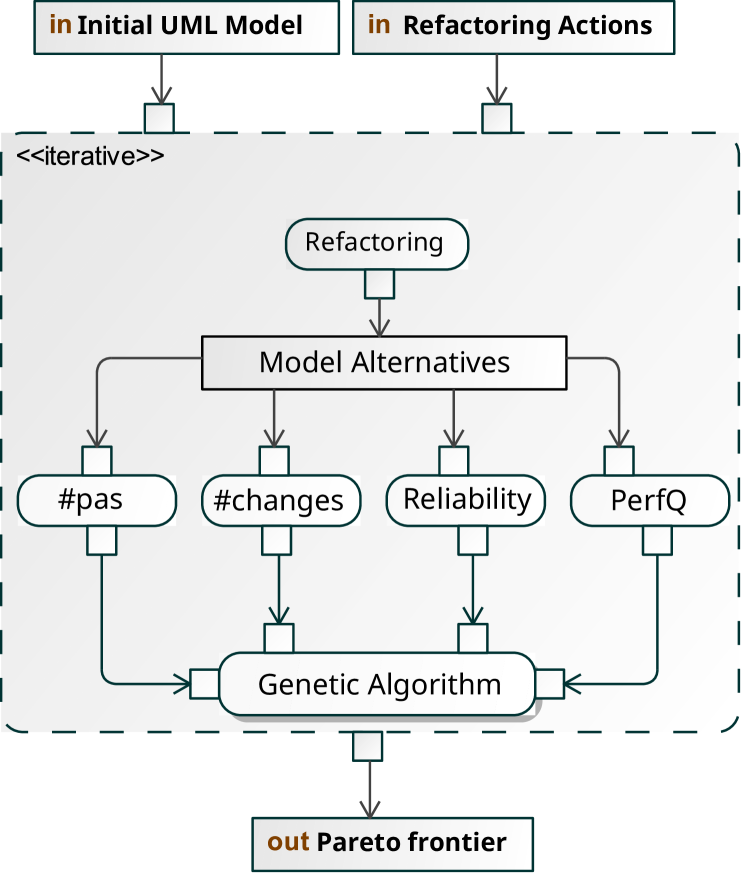
Figure 1: The graphical representation of the approach. The approach takes as input: the set of all the available refactoring actions (Refactoring Actions), and the subject model (Initial UML Model). The Genetic Algorithm (i.e., NSGA-II, SPEA2, and PESA2) randomly selects and combines refactoring actions (Refactoring) in order to build a set of Model Alternatives. #pas, #changes, reliability, and perfQ are the four objectives that drive the optimization process.

Performance Quality Indicator (perfQ)

perfQ quantifies the performance improvement/detriment between two models. Furthermore, a single perfQ for each performance index is computed as the normalized ratio between the index value of a model alternative and the initial model. Finally, the global perfQ is computed as the average across the number of performance indices considered in the performance analysis.

Reliability model

The reliability model that we adopt here to quantify the reliability objective is based on the model introduced in [29].

The model takes into account failure probabilities of components and communication links, as well as the probability of a scenario to be executed. Such probabilities are combined to obtain the overall reliability on demand of the system, which represents how often the system is not expected to fail when its scenarios are invoked.

Performance Antipatterns

A performance antipattern describes bad design practices that might lead to performance degradation in a system. These textual descriptions were later translated into first-order logic (FOL) equations [30].

FOLs enable an automated comparison with thresholds in order to reveal the occurrences of a performance antipattern. The identification of such thresholds is a non-trivial task, and using deterministic values may result in an excessively strict detection, where the smallest change in the value of a literal determines the occurrence of the antipattern. For these reasons, we use the fuzzy threshold concept [30], instead of detecting a performance antipattern in a deterministic way. By using fuzzy thresholds, we assign probabilities to the occurrences of antipatterns.

Architectural distance

The architectural distance #changes quantifies the distance of the model obtained by applying refactoring actions to the initial one. The effort needed to perform a refactoring is quantified as the product between the baseline refactoring factor, which is associated to each refactoring action, and the architectural weight, which is associated to each model element on the basis of the number of connections to other elements in the model [9]. The overall #changes is obtained by summing the efforts of all refactoring actions contained in a solution.

Hypervolume

Establishing the quality of a computed Pareto front is arduous, and it is a NP-hard problem [31]. Different quality estimators have been introduced, such as the Hypervolume (HV) [13, 12]. Each estimator measures a different quality aspect of a Pareto front. In this study, we use the HV as our quality estimator, since it has been proved to be a valid estimator for Pareto fronts comparison [32]. Moreover, the HV interpretation is straightforward in the context of our problem.

The HV measures the amount of the volume of the solution space that a Pareto front ($PF^{c}$) covers with respect to a reference Pareto front ($PF^{ref}$), and it can assume values between $0$ and $1$. When the $HV=0$, it means that the $PF^{c}$ is fully dominated by the $PF^{ref}$, while $HV=1$ means that each point within the $PF^{c}$ is non-dominated by any points within the $PF^{ref}$. Therefore, the closer to 1 the HV, the higher the quality of the $PF^{c}$. In our evaluation, we use the HV to estimate the quality of the $PF^{c}$ obtained with a search budget when compared to a $PF^{ref}$ computed without, but terminated after 102 evolutions.

IV Study Design

The goal of the study is to establish how much the imposition of a time-based search budget can hamper the quality of the resulting Pareto fronts in a model-based multi-objective refactoring optimization context. Additionally, we are interested in how different algorithms cope with different search budgets. To this extent, we selected two case studies, and we run the optimization with search budgets of 15, 30, and 60 minutes. Moreover, for each search budget, we also run three genetic algorithms: NSGA-II, SPEA2, and PESA2. We chose these three algorithms on the basis of their different searching policies, as described in Section III.

As recommended in other studies [33], because of the random nature of genetic algorithms, we run the same experiment 31 times, and we compute the HV for each computed Pareto front ($PF^{c}$). The HV indicator measures the amount of volume in the solution space that is covered by a $PF^{c}$ with respect to an optimal reference Pareto front ($PF^{ref}$) for the problem. Since $PF^{ref}$ is unknown in our case studies, we computed the HV with respect to the best Pareto front we obtained for the same case studies when we run the search for 102 evolutions without a search budget. The entire study consisted of 558 experiments that we performed on three AMD EPYC 7282, each with 64 cores and 512GB of RAM.

We follow the guidelines by Arcuri et al. [34] to compare the experiments against each other. Therefore, we apply the Mann–Whitney U non-parametric statistical test (also referred to as Wilcoxon rank-sum test) [35] with the null hypothesis that the experiments do not show a statistically significant difference. We consider two experiments to be significantly different on the basis of their HV if the test computes a p-values smaller than $0.05$. To assess the magnitude of the difference, we use the Vargha–Delaney $\hat{A}_{12}$ [36], a standardized non-parametric effect size measure. $\hat{A}_{12}$ takes values between $0$ and $1$, and a values of $0.5$ indicates that the two experiments are equivalent. The closer the value of $\hat{A}_{12}$ gets to $0$ or $1$, the larger the effect. The interpretation of the magnitude as negligible, small, medium, and large is performed according to the thresholds $0.147$, $0.33$, $0.474$ [37].

V Empirical Evaluation

In this section, we present the results of our experiments, and we answer the research questions formulated in Section I.

V-A Case Study

We applied our optimization approach to two case studies from the literature: the Train Ticket Booking Service (TTBS) [14], and the well-established modeling case study CoCoME, whose UML model has been derived by the specification in [15].

Train Ticket Booking Service

Train Ticket Booking Service (TTBS) is a web-based booking application, whose architecture is based on the microservice paradigm. The system is made up of 40 microservices, and it provides different scenarios through users that can perform realistic operations, e.g., book a ticket or watch trip information.

For our analysis we downsized the TTBS UML model [14] by considering 11 UML Components, 11 UML Nodes, and 3 UML Use Cases. Furthermore, we considered Login, Update user details and Rebook as selected scenarios because they commonly represent performance-critical scenarios in a ticketing booking service. Also, the model defines two user categories: simple and admin users.

CoCoME

CoCoME describes a trading system containing several stores. A store can have one or more cash desks for processing goods. A cash desk is equipped with all the tools needed to serve a customer (e.g., a Cash Box, Printer, Bar Code Scanner). CoCoME covers possible scenarios performed at a cash desk (e.g., scanning products, paying by credit card, or ordering new goodies). CoCoME describes 8 scenarios involving more than 20 components.

For our analysis, we downsized CoCoME by selecting 3 UML Use Cases, 13 UML Components, and 8 UML Nodes. Beside this, we focused on three scenarios: Process Sale, Receive Ordered Products, and Show stock reports because they represent common activities in a trading system.

V-B RQ1

RQ1: To what extent does the time budget penalize the quality of Pareto fronts?

The first main concern on the imposition of a search budget is the effect this can have on the optimization process. As outlined in Section IV, we estimate the impact a search budget has on the optimization by means of the HV quality indicator. Table I reports, for each algorithm and for each search budget, the average HV achieved in 31 runs, along with its standard deviation. These value represent the percentage of volume of the $PF^{ref}$ that is covered by a give $PF^{c}$. Intuitively, this gives an idea of how much of the solution space was covered with the budget restriction, compared to a run without the search budget. We can observe that, in fact, the time budget heavily impacts the quality of the obtained Pareto fronts.

Algor.	Budget	HV avg	HV stdev
TTBS ($\Omega=1.2\times 10^{13}$)
NSGA-II	15 min	0.3060	0.0915
NSGA-II	30 min	0.3469	0.1071
NSGA-II	60 min	0.3437	0.0980
PESA2	15 min	0.3532	0.0794
PESA2	30 min	0.4084	0.0757
PESA2	60 min	0.4182	0.0819
SPEA2	15 min	0.3041	0.0794
SPEA2	30 min	0.2917	0.0920
SPEA2	60 min	0.2868	0.0769
CoCoME ($\Omega=3.26\times 10^{16}$)
NSGA-II	15 min	0.0931	0.0335
NSGA-II	30 min	0.1199	0.0523
NSGA-II	60 min	0.1125	0.0604
PESA2	15 min	0.1363	0.0277
PESA2	30 min	0.1460	0.0300
PESA2	60 min	0.1514	0.0366
SPEA2	15 min	0.1189	0.0336
SPEA2	30 min	0.1098	0.0309
SPEA2	60 min	0.1023	0.0384

Table I: Average HV quality indicator and its standard deviation over 31 runs, listed by algorithm and search budget. Higher values are associated to a better quality of the Pareto fronts. $\Omega$ is the size of the solution space computed as the Cartesian product of the types of refactoring actions and all the eligible refactoring targets in any possible refactoring sequence.

The search budget had a different impact on the two case studies. In TTBS, the search was able to achieve better HV in all cases, when compared to CoCoME. This is probably due to the difference in size and complexity between the two case studies. CoCoME not only has a larger number of possible refactoring candidates, but its model defines a more complex behavior. This inherently leads to a bigger solution space ($\Omega$ in the table), but also to spending more time in computing the objective functions. Therefore, on average, the longer it takes to complete a single evolution, the fewer the evolutions will be performed on a given time budget.

To assess whether doubling or quadrupling the time budget makes a significant difference in the HV of the $PF^{c}$, we compare the results obtained with different budgets but with the same algorithm. Table II reports the results of the Mann–Whitney U test, and the corresponding $\hat{A}_{12}$ effect size. The p-value is highlighted in bold when the detected difference is statistically significant. The time budget is underlined when (i) the test resulted in a significant difference, and (ii) the experiment running on that time budget produced higher values of HV. In very few cases (two per case study), we obtained a significant difference, and in all the cases this was detected for the PESA2 algorithm: with a medium magnitude in TTBS, and with a large one in CoCoME. This suggests that, except for PESA2, the main difference in the obtained HV values might be imputed to a difference in the used algorithm, more than to a difference in the budget. We are going to investigate this in the next section.

Algor.	Budget 1	Budget 2	MWU p	$\hat{A}_{12}$
TTBS
NSGA-II	15 min	30 min	0.1677	(S) 0.3975
NSGA-II	15 min	60 min	0.1677	(S) 0.3975
NSGA-II	30 min	60 min	0.9327	(N) 0.5068
PESA2	15 min	30 min	0.018	(M) 0.3247
PESA2	15 min	60 min	0.0031	(M) 0.281
PESA2	30 min	60 min	0.4223	(N) 0.4402
SPEA2	15 min	60 min	0.4992	(N) 0.5505
SPEA2	30 min	15 min	0.4556	(N) 0.4443
SPEA2	30 min	60 min	0.7999	(N) 0.4807
CoCoME
NSGA-II	15 min	30 min	0.0574	(S) 0.359
NSGA-II	60 min	15 min	0.1054	(S) 0.6202
NSGA-II	60 min	30 min	0.8769	(N) 0.488
PESA2	15 min	30 min	$<$0.0001	(L) 0.2092
PESA2	60 min	15 min	$<$0.0001	(L) 0.7992
PESA2	60 min	30 min	0.6024	(N) 0.539
SPEA2	30 min	15 min	0.2483	(S) 0.4142
SPEA2	60 min	15 min	0.1249	(S) 0.3861
SPEA2	60 min	30 min	0.6123	(N) 0.462

Table II: Mann–Whitney U test and $\hat{A}_{12}$ effect sizes comparing the HV achieved with different time budgets in 31 runs. Magnitude interpretation: negligible (N), small (S), medium (M), large (L). The magnitude of the effect size is also represented by bars.

V-C RQ2

RQ2: Which algorithm performs better when limited by a time budget?

When a time constraint is imposed on the process, a designer may be interested in selecting the algorithm that provides best quality solutions for the specific time budget. In this section, we discuss some aspects on which such a decision could be based.

At first, we compare the algorithms against each other on the basis of the HV they achieved in the experiments, analogously to how it has been done in Section V-B. Table III reports the results of the Mann–Whitney U test, and the corresponding $\hat{A}_{12}$ effect size. The name of the algorithm is underlined when (i) the test resulted in a significant difference, and (ii) that algorithm yielded higher values of HV. In this case, most of the tests revealed a significant difference between the algorithms in any given time budget (highlighted in bold). PESA2 performed better in many cases and in both case studies, NSGA-II scored better on only two cases in TTBS and not by a large margin, and SPEA2 won only the 15 minutes budget test in CoCoME.

Budget	Algor. 1	Algor. 2	MWU p	$\hat{A}_{12}$
TTBS
15 min	PESA2	NSGA-II	0.0487	(S) 0.6462
15 min	SPEA2	NSGA-II	0.8548	(N) 0.486
15 min	SPEA2	PESA2	0.0234	(M) 0.3319
30 min	NSGA-II	PESA2	0.0167	(M) 0.3226
30 min	SPEA2	NSGA-II	0.0385	(S) 0.3465
30 min	SPEA2	PESA2	$<$0.0001	(L) 0.1582
60 min	NSGA-II	PESA2	0.0037	(M) 0.2851
60 min	SPEA2	NSGA-II	0.0202	(M) 0.3278
60 min	SPEA2	PESA2	$<$0.0001	(L) 0.1301
CoCoME
15 min	NSGA-II	SPEA2	0.0085	(M) 0.3049
15 min	PESA2	NSGA-II	0.0072	(M) 0.6993
15 min	PESA2	SPEA2	0.7999	(N) 0.4807
30 min	PESA2	NSGA-II	0.0066	(M) 0.7014
30 min	SPEA2	NSGA-II	0.5543	(N) 0.4558
30 min	SPEA2	PESA2	$<$0.0001	(L) 0.1738
60 min	PESA2	NSGA-II	0.0127	(M) 0.6847
60 min	SPEA2	NSGA-II	0.3789	(N) 0.4344
60 min	SPEA2	PESA2	$<$0.0001	(L) 0.1686

Table III: Mann–Whitney U test and $\hat{A}_{12}$ effect sizes comparing the HV achieved by different algorithms in 31 runs. Magnitude interpretation: negligible (N), small (S), medium (M), large (L). The magnitude of the effect size is also represented by bars.

While the results vary in the two case studies we considered, the PESA2 algorithm looks like a better choice in most cases. To investigate the possible reasons behind such differences in HV, we take a look at how the HV is achieved and when, by comparing it to the time budget and the number of performed evolutions. To this extent, Figure 2 depicts the timelines of how the HV indicator varies with different search budgets, and how many evolutions were performed during the search. From the timelines, we can see that SPEA2 is the slowest algorithm in our experiments, whereas NSGA-II is the fastest one. Furthermore, for each search budget, NSGA-II performed the highest number of evolutions, e.g., it performed on average 20 evolutions for TTBS with 60 minutes of search budget, and almost 18 for CoCoME. Conversely, SPEA2 performed, on average, only 8 evolutions for TTBS with a 60 minutes search budget. Concerning the PESA2 algorithm, we can state that it consistently generated the highest HV in each case study and for every search budget. However, it is slower than NSGA-II, but faster than SPEA2.

Analyzing the TTBS results, we observed that the HV values of SPEA2 almost lie close to $0.3$ fore every search budget, while the longer the search budget, the higher the HV values of PESA2. The HV values of NSGA-II increase between the 15 and 30 minutes budget, while they are almost flat between 30 and 60 minutes. In addition, we can observe that the timelines of the two case studies resemble each other. In fact, also per CoCoME, NSGA-II is the fastest algorithm, SPEA2 the slowest, and PESA2 generates the highest HV values. Furthermore, the number of evolutions are consistent with the number of evolutions of TTBS.

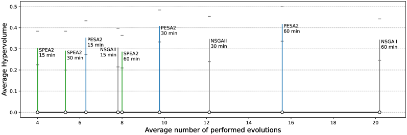
(a) TTBS

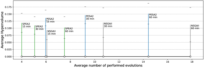
(b) CoCoME

Figure 2: Timelines of the number of evolutions performed by the algorithms in the different budget configurations, along with the achieved HV. Vertical bars show the average HV over 31 runs, and ticks represent the standard deviation from the mean.

Another viewpoint on the difference among the algorithms could be the actual quality of the computed solutions in terms of the non-functional properties we are interested in. To visually inspect this aspect, we produced scatter plots to compare perfQ and reliability, because these objectives are the non-functional properties we aim at improving through the refactoring and optimization process. Therefore, Figure 3(a), Figure 3(b), and Figure 3(c) depict the three $PF^{c}$ when varying the time budget of all three genetic algorithms for both case studies. At a glance, we can observe more densely populated $PF^{c}$ for CoCoME than for TTBS, while TTBS showed a more evident trend towards the top-right corner (the optimization direction for these two objectives). Regarding the CoCoME $PF^{c}$, we can observe an horizontal clustering for the three search budgets. The cluster that lies around $0.8$ reliability is always more populated that the other two: one between $0.4$ and $0.6$, and the other between $0.0$ and $0.2$, approximately. We did not observe an evident motivation for the horizontal clustering of CoCoME. We can only suppose that the characteristics of the CoCoME model, which has a more complex behavior than TTBS, prevent the algorithms from reaching higher reliability values in the search budgets we considered. Also, the CoCoME solution space might be less homogeneous, with feasible solutions that are inherently clustered.

Summarizing, on the one hand we can establish a clear difference among the algorithms when comparing them on the basis of a quality indicator for multi-objective optimization, like the HV, and when looking at their speed in completing evolutions. But on the other hand, if we only look at the non-functional properties we considered, there is not much difference in the shape of the $PF^{c}$ and in the explored design space.

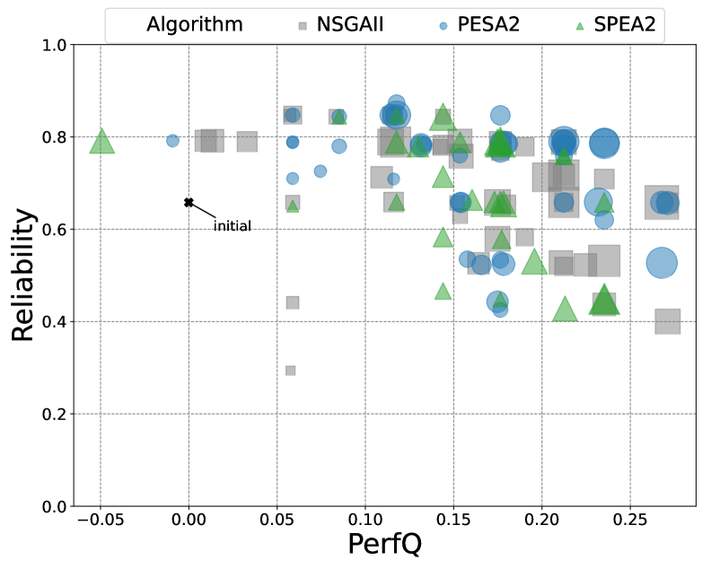
TTBS CoCoME

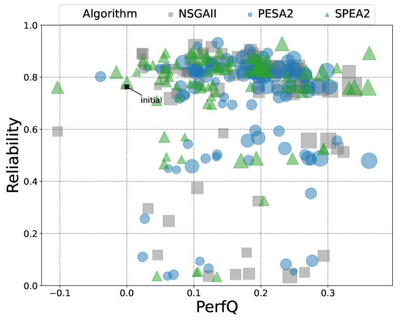
(a) 15 min budget

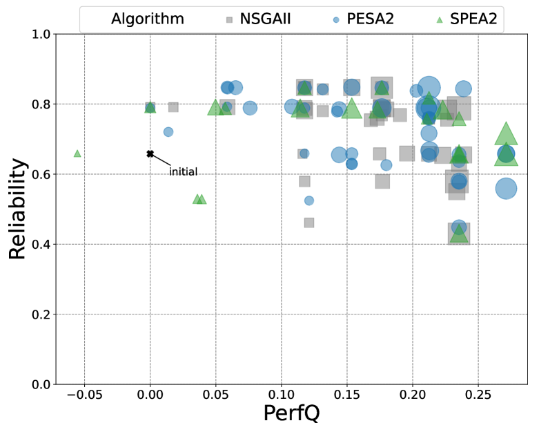
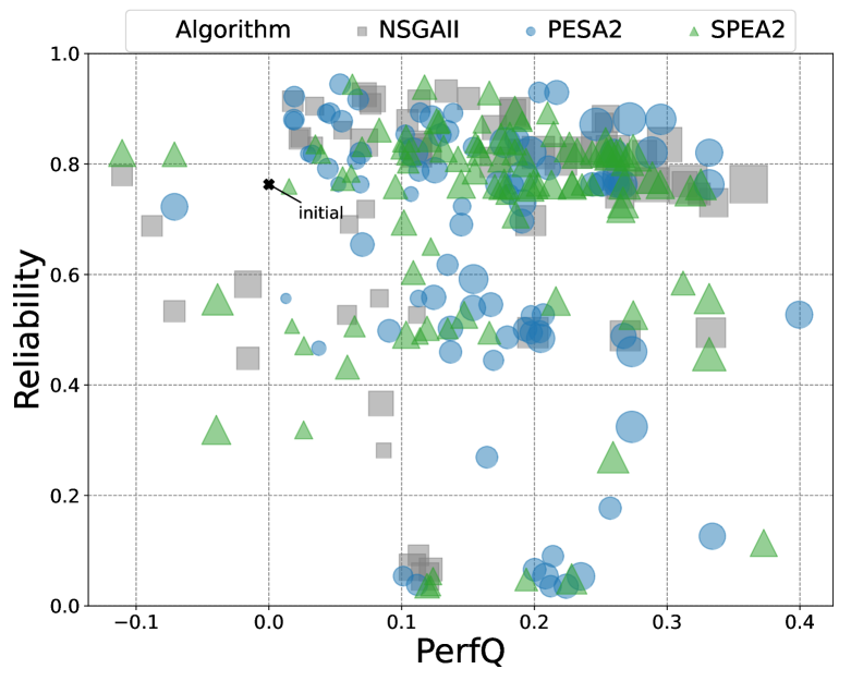
(b) 30 min budget

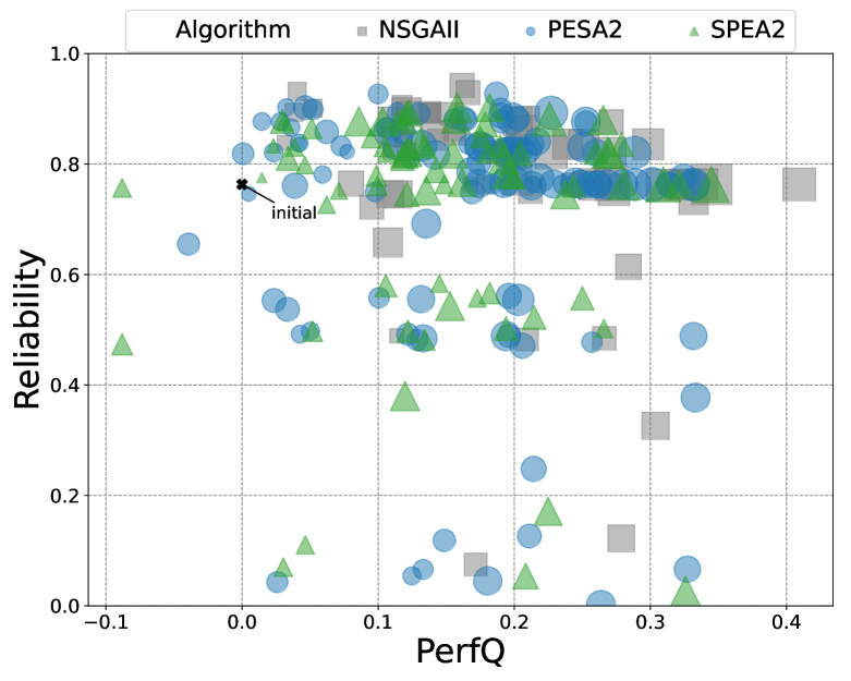
(c) 60 min budget

Figure 3: TTBS, and CoCoME Pareto frontiers obtained by the three algorithms when varying the time budget between 15, 30, and 60 minutes. The top-right corner is the optimal point, whereas the bottom-left corner is the worst one. Filled symbols are the three algorithms: NSGA-II is the gray squares, PESA2 is the blue circles, and SPEA2 is the green triangles.

V-D Threats to validity

In this section we discuss threats that might affect our results.

Construct validity

Our approach might be affected by Construct validity threats. An aspect that might affect our results is the estimation of the reference Pareto front ($PF^{ref}$). $PF^{ref}$ is used to extract the quality indicators, as described in Section IV. We mitigate this threat by building the $PF^{ref}$ from a run without the search budget for each case study. Therefore, $PF^{ref}$ should contain all the non-dominated solutions across all configurations, and it should also represent a good Pareto front for computing the HV indicator.

External validity

Our approach might be affected by external validity threats, because we have used a single modeling notation. We cannot generalize our results to other modeling notations, which could imply using a different portfolio of refactoring actions. In fact, the syntax and semantics of the modeling notation determine the amount and nature of refactoring actions that can be performed. We could mitigate these threats, for example, by using another modeling notation.

Internal Validity

Our results might be affected by Internal validity threats. One aspect that might affect our findings is a misleading interpretation of the outcome due to the random nature of genetic algorithms. In order to mitigate the internal validity threats, we performed 31 executions for each configuration [33].

Conclusion validity

Our results might be affected by Conclusion validity threats, since our considerations might change with better-tuned parameters for each algorithm. We did not perform an extensive tuning phase for each algorithm. However, we used common parameters to setup the algorithms, which should mitigate these threats [38]. Wherever possible, we used appropriate statistical procedures with p-value and effect size measures to test the significance of the differences and their magnitude.

VI Lesson learned

We learned that it is not always possible to select a genetic algorithm beforehand. The selection of the algorithm is strictly related to the domain and the policy for searching the solution space. Furthermore, the selection becomes even more complex when a search budget limits the search.

Our initial investigation shed light on which algorithm is faster among the studied ones and which algorithm has been able to produce better quality Pareto fronts when the search has a time limitation. Based on our investigation, we understand that the NSGA-II policy of non-dominated knowledge helps the algorithm to perform more evolutions. In contrast, the hyper-grid searching policy exploited by PESA2 allows the algorithm to generate the Pareto fronts with the highest quality. Finally, SPEA2, in our experimentation, showed speed and quality limitations due to the usage of two archives for storing Pareto solutions.

We also learned that the application domain is the most driving aspect of genetic algorithms. In fact, from our results, in one case, we had horizontal clusters (see CoCoME on Figure 3), which were likely due to the more complex nature of the subject model. Our results showed a more precise optimization direction for two objectives in the other case.

As a final takeaway, small time budgets could be used in preliminary experiments designed to compare the algorithms and to select the best one for the longer runs.

VII Conclusion and Future Work

In this study we presented an investigation on the impact of the search budget for model-based multi-objective refactoring optimization. The study was aimed at helping designers to select the best algorithm with respect to the search budget. In addition, we validated the study on two model benchmarks, Train Ticket Booking Service, and CoCoME, and on three genetic algorithms, NSGA-II, SPEA2, and PESA2.

We assessed the overall quality of each algorithm through the Hypervolume indicator, which measures the amount of the search space volume that a computed Pareto front covers with respect to the reference Pareto front. From our results, it emerges that NSGA-II is the fastest algorithm because it generated the highest number of evolution genetic within the search budget. PESA2 is the algorithm that generated the highest quality results in terms of HV. Finally, SPEA2 is the slowest algorithm, and it generated the worst quality results. Thus, it generated the lowest number of genetic evolutions, and showed the lowest HV values.

As future work, we intend to analyze the Pareto front at each evolution in order to discover if the quality is not improving enough, and we could just stop the algorithm.

References

- [1] A. Ramírez, J. R. Romero, and S. Ventura, “A survey of many-objective optimisation in search-based software engineering,” JSS, vol. 149, pp. 382–395, 2019.
- [2] T. Mariani and S. R. Vergilio, “A systematic review on search-based refactoring,” JIST, vol. 83, pp. 14–34, Mar. 2017.
- [3] A. Ouni, M. Kessentini, K. Inoue, and M. Ó Cinnéide, “Search-Based Web Service Antipatterns Detection,” TSC, vol. 10, no. 4, pp. 603–617, 2017.
- [4] G. Bavota, M. Di Penta, and R. Oliveto, “Search Based Software Maintenance: Methods and Tools,” in Evol. Soft. Sys., 2014, pp. 103–137.
- [5] V. Cortellessa and D. Di Pompeo, “Analyzing the sensitivity of multi-objective software architecture refactoring to configuration characteristics,” JIST, vol. 135, p. 106568, 2021.
- [6] A. Aleti, S. Björnander, L. Grunske, and I. Meedeniya, “ArcheOpterix: An extendable tool for architecture optimization of AADL models,” in ICSE MOMPES Workshop, 2009, pp. 61–71.
- [7] A. Martens, H. Koziolek, S. Becker, and R. H. Reussner, “Automatically improve software architecture models for performance, reliability, and cost using evolutionary algorithms,” in ICPE 2010 - Proceedings of the 1st ACM/SPEC International Conference on Performance Engineering. New York, New York, USA: ACM Press, 2010, pp. 105–116.
- [8] C. Blum and A. Roli, “Metaheuristics in combinatorial optimization: Overview and conceptual comparison,” ACM Comput. Surv., vol. 35, no. 3, pp. 268–308, 2003.
- [9] V. Cortellessa, D. Di Pompeo, V. Stoico, and M. Tucci, “On the impact of performance antipatterns in multi-objective software model refactoring optimization,” in SEAA, 2021, p. 224–233. [Online]. Available: \urlhttps://ieeexplore.ieee.org/document/9582578/
- [10] A. Arcuri and G. Fraser, “On parameter tuning in search based software engineering,” in Search Based Software Engineering, ser. LNCS, M. B. Cohen and M. Ó Cinnéide, Eds., vol. 6956. Springer Berlin Heidelberg, 2011, p. 33–47. [Online]. Available: \urlhttp://link.springer.com/10.1007/978-3-642-23716-4_6
- [11] D. Arcelli, V. Cortellessa, M. D’Emidio, and D. Di Pompeo, “EASIER: an Evolutionary Approach for multi-objective Software archItecturE Refactoring,” in ICSA, 2018, pp. 1–10.
- [12] N. Beume, B. Naujoks, and M. Emmerich, “Sms-emoa: Multiobjective selection based on dominated hypervolume,” European Journal of Operational Research, vol. 181, no. 3, pp. 1653 – 1669, 2007.
- [13] Y. Cao, B. J. Smucker, and T. J. Robinson, “On using the hypervolume indicator to compare Pareto fronts: Applications to multi-criteria optimal experimental design,” Journal of Statistical Planning and Inference, vol. 160, pp. 60–74, May 2015.
- [14] D. Di Pompeo, M. Tucci, A. Celi, and R. Eramo, “A microservice reference case study for design-runtime interaction in MDE,” in STAF MDE@DeRun Workshop, vol. 2405, 2019, pp. 23–32.
- [15] S. Herold, H. Klus, Y. Welsch, C. Deiters, A. Rausch, R. Reussner, K. Krogmann, H. Koziolek, R. Mirandola, B. Hummel, M. Meisinger, and C. Pfaller, CoCoME - The Common Component Modeling Example, ser. lncs. Springer Berlin Heidelberg, 2008, vol. 5153, p. 16–53. [Online]. Available: \urlhttp://link.springer.com/10.1007/978-3-540-85289-6_3
- [16] K. Deb, A. Pratap, S. Agarwal, and T. Meyarivan, “A fast and elitist multiobjective genetic algorithm: NSGA-II,” TEVC, vol. 6, no. 2, pp. 182–197, Apr. 2002.
- [17] E. Zitzler, M. Laumanns, and L. Thiele, “Spea2: Improving the strength pareto evolutionary algorithm,” Swiss Federal Institute of Technology (ETH) Zurich, TIK-report 103, 2001.
- [18] D. W. Corne, N. R. Jerram, J. D. Knowles, and M. J. Oates, “Pesa-ii: Region-based selection in evolutionary multiobjective optimization,” in Proceedings of the 3rd Annual Conference on Genetic and Evolutionary Computation, ser. GECCO’01. Morgan Kaufmann Publishers Inc., 2001, p. 283–290, event-place: San Francisco, California.
- [19] R. Li, R. Etemaadi, M. T. M. Emmerich, and M. R. V. Chaudron, “An evolutionary multiobjective optimization approach to component-based software architecture design,” in CEC. IEEE, 2011, pp. 432–439.
- [20] I. Meedeniya, B. Buhnova, A. Aleti, and L. Grunske, “Architecture-Driven Reliability and Energy Optimization for Complex Embedded Systems,” in QoSA. Springer, 2010, pp. 52–67.
- [21] A. Martens, D. Ardagna, H. Koziolek, R. Mirandola, and R. H. Reussner, “A Hybrid Approach for Multi-attribute QoS Optimisation in Component Based Software Systems,” in Research into Practice – Reality and Gaps, 2010, pp. 84–101.
- [22] V. Cardellini, E. Casalicchio, V. Grassi, F. Lo Presti, and R. Mirandola, “QoS-driven Runtime Adaptation of Service Oriented Architectures,” in ESEC/FSE, 2009, pp. 131–140.
- [23] Y. Ni, X. Du, P. Ye, L. L. Minku, X. Yao, M. Harman, and R. Xiao, “Multi-objective software performance optimisation at the architecture level using randomised search rules,” JIST, vol. 135, p. 106565, 2021.
- [24] A. Rago, S. A. Vidal, J. A. Diaz-Pace, S. Frank, and A. van Hoorn, “Distributed quality-attribute optimization of software architectures,” in SBCARS, 2017, pp. 7:1–7:10.
- [25] S. Becker, H. Koziolek, and R. H. Reussner, “The Palladio component model for model-driven performance prediction,” Systems and Software, vol. 82, no. 1, pp. 3–22, Jan. 2009.
- [26] D. A. Menascé, J. M. Ewing, H. Gomaa, S. Malek, and J. P. Sousa, “A framework for utility-based service oriented design in SASSY,” in WOSP/SIPEW, 2010, pp. 27–36.
- [27] P. H. Feiler and D. P. Gluch, Model-Based Engineering with AADL - An Introduction to the SAE Architecture Analysis and Design Language, ser. SEI series in software engineering. Addison-Wesley, 2012.
- [28] V. Cortellessa, R. Eramo, and M. Tucci, “From software architecture to analysis models and back: Model-driven refactoring aimed at availability improvement,” Inf. Softw. Technol., vol. 127, p. 106362, 2020.
- [29] V. Cortellessa, H. Singh, and B. Cukic, “Early reliability assessment of UML based software models,” in WOSP@ISSTA, 2002, pp. 302–309.
- [30] D. Arcelli, V. Cortellessa, and C. Trubiani, “Performance-based software model refactoring in fuzzy contexts,” in FASE, 2015, pp. 149–164.
- [31] S. Ali, P. Arcaini, D. Pradhan, S. A. Safdar, and T. Yue, “Quality indicators in search-based software engineering: An empirical evaluation,” ACM Transactions on Software Engineering and Methodology, vol. 29, no. 2, p. 1–29, 2020. [Online]. Available: \urlhttps://dl.acm.org/doi/10.1145/3375636
- [32] J. G. Falcón-Cardona and C. A. C. Coello, “Indicator-based multi-objective evolutionary algorithms: A comprehensive survey,” ACM Computing Surveys, vol. 53, no. 2, p. 1–35, Mar 2021. [Online]. Available: \urlhttps://dl.acm.org/doi/10.1145/3376916
- [33] E. Zitzler, K. Deb, and L. Thiele, “Comparison of multiobjective evolutionary algorithms: Empirical results,” Evolutionary Computation, vol. 8, no. 2, p. 173–195, 2000. [Online]. Available: \urlhttps://direct.mit.edu/evco/article/8/2/173-195/868
- [34] A. Arcuri and L. C. Briand, “A hitchhiker’s guide to statistical tests for assessing randomized algorithms in software engineering,” Softw. Test. Verification Reliab., vol. 24, no. 3, pp. 219–250, 2014. [Online]. Available: \urlhttps://doi.org/10.1002/stvr.1486
- [35] H. B. Mann and D. R. Whitney, “On a Test of Whether one of Two Random Variables is Stochastically Larger than the Other,” The Annals of Mathematical Statistics, vol. 18, no. 1, pp. 50 – 60, 1947. [Online]. Available: \urlhttps://doi.org/10.1214/aoms/1177730491
- [36] A. Vargha and H. D. Delaney, “A critique and improvement of the ”cl” common language effect size statistics of mcgraw and wong,” Journal of Educational and Behavioral Statistics, vol. 25, no. 2, pp. 101–132, 2000. [Online]. Available: \urlhttp://www.jstor.org/stable/1165329
- [37] M. Hess and J. Kromrey, “Robust confidence intervals for effect sizes: A comparative study of cohen’s d and cliff’s delta under non-normality and heterogeneous variances,” American Educational Research Association, 01 2004.
- [38] A. Arcuri and G. Fraser, “Parameter tuning or default values? an empirical investigation in search-based software engineering,” Empirical Software Engineering, vol. 18, no. 3, pp. 594–623, 2013.