Instance-specific Label Distribution Regularization for Learning with Label Noise

Abstract

Modeling noise transition matrix is a kind of promising method for learning with label noise. Based on the estimated noise transition matrix and the noisy posterior probabilities, the clean posterior probabilities, which are jointly called Label Distribution (LD) in this paper, can be calculated as the supervision. To reliably estimate the noise transition matrix, some methods assume that anchor points are available during training. Nonetheless, if anchor points are invalid, the noise transition matrix might be poorly learned, resulting in poor performance. Consequently, other methods treat reliable data points, extracted from training data, as pseudo anchor points. However, from a statistical point of view, the noise transition matrix can be inferred from data with noisy labels under the clean-label-domination assumption. Therefore, we aim to estimate the noise transition matrix without (pseudo) anchor points. There is evidence showing that samples are more likely to be mislabeled as other similar class labels, which means the mislabeling probability is highly correlated with the inter-class correlation. Inspired by this observation, we propose an instance-specific Label Distribution Regularization (LDR), in which the instance-specific LD is estimated as the supervision, to prevent DCNNs from memorizing noisy labels. Specifically, we estimate the noisy posterior under the supervision of noisy labels, and approximate the batch-level noise transition matrix by estimating the inter-class correlation matrix with neither anchor points nor pseudo anchor points. Experimental results on two synthetic noisy datasets and two real-world noisy datasets demonstrate that our LDR outperforms existing methods.

1 Introduction

The success of deep convolutional neural networks (DCNNs) relies heavily on a myriad amount of accurately labeled training data. However, due to the intensive annotation cost and inter-annotator variability, most collected datasets inevitably contain label noise yu2018learning , $i.e.$, the observed labels of samples might be wrong, particularly when the size of datasets is large. Since a DCNN is capable of memorizing randomly labeled data Zhang2017UnderstandingDL , it tends to overfit noisy labels, leading to poor performance and generalizability. Therefore, designing an effective method to improve the robustness of DCNNs against noisy labels is of great practical significance.

Many research efforts have been devoted to learning with label noise, resulting in a number of solutions. Most of them attempt to first filter the samples with noisy labels and then reduce the impact of those samples han2018co ; li2019dividemix ; wang2022scalable ; xia2020robust ; kim2019nlnl ; thulasidasan2019combating ; patrini2017making ; xia2022sample ; Huang2022UncertaintyAwareLA . Although these methods avoid the complex modeling of label noise, they have limited reliability, since the classifier learned on data with label noise may not be statistically consistent (i.e., it can hardly guarantee that the noisy-label-trained classifier approaches the optimal classifier defined on the clean risk) li2021provably .

To overcome this limitation, more and more methods choose to model label noise explicitly cheng2022instance ; li2021provably . Particularly, the most popular strategy, which theoretically guarantees the statistical consistency, is to convert the noisy posterior probabilities $P(Y\mid\textbf{x})$ into a clean one $P(Y^{*}\mid\textbf{x})$ based on the noise transition matrix and then use the clean posterior probabilities as supervision to guide the training process hendrycks2018using ; li2021provably ; xia2019anchor ; shu2020meta ; yao2020dual ; cheng2020learning ; cheng2022instance ; berthon2021confidence ; xia2020part ; yang2021estimating . $Y$ and $Y^{*}$ represent the observed label and the unseen GT label, and the clean posterior $P(Y^{*}\mid\textbf{x})$ is called Label Distribution (LD) in this paper. Obviously, estimating the noise transition matrix is the most essential and challenging step xia2019anchor . To reliably estimate the noise transition matrix, some methods assume that a small anchor point set is available during training hendrycks2018using ; shu2020meta ; berthon2021confidence ; xia2020part . Note that anchor points are training samples that we know are correctly labeled. Nonetheless, the anchor point assumption limits the application of those fore-mentioned methods. If anchor points are invalid, the noise transition matrix might be poorly learned xia2020part , resulting in poor performance. Consequently, other methods treat reliable data points, extracted from training data, as the pseudo anchor points xia2019anchor ; yao2020dual ; cheng2022instance . These noise transition matrix estimating methods use the anchor points or pseudo anchor points because of the concern that the estimation might be misguided by wrong annotations shu2020meta ; xia2020part . However, from a statistical point of view, the noise transition matrix can be inferred from data with noisy labels under the clean-label-domination assumption. Note that the clean-label-domination assumption is that samples have a higher probability to be annotated with GT labels than any other class labels zhou2021asymmetric . As a consequence, we aim to estimate the noise transition matrix without either anchor points or pseudo anchor points. There is some evidence showing that samples are more likely to be mislabeled as other similar class labels cohen2020separability ; beyer2020we , which means the mislabeling probability is highly correlated with the inter-class correlation. It points out a way to approximate the noise transition matrix, $i.e.$, estimating the inter-class correlation.

To this end, we propose a simple and effective regularization, named Label Distribution Regularization (LDR), to alleviate the negative impact of label noise. Overall, for each training sample, we estimate the instance-specific LD base on the estimated noise transition matrix and the estimated noisy posterior probabilities, and then utilize the estimated instance-specific LD as the supervision. Specifically, noisy posterior $P\left(Y\mid\textbf{x}\right)$ is easy to be estimated under the supervision of noisy labels. The noise transition matrix $P\left(Y^{*}\mid Y\right)$ is approximated by estimating the batch-level inter-class correlation matrix, which is more accurate than estimating the inter-class correlation matrix of the dataset. The batch-level inter-class correlation matrix is the column Gram Matrix gatys2016neural of the prediction of the classifier in each mini-batch. Based on these two steps, the instance-specific LD $P\left(Y^{*}\mid\textbf{x}\right)$ can be calculated. To further minimize the impact of noise, the estimated instance-specific LD is sharpened at the end. In addition, when trained on noisy datasets, DCNNs have been observed to first fit data with clean labels during an early learning phase, before eventually memorizing the samples with false labels liu2020early , so that the model begins by learning to predict the true labels, even for many of the samples with the wrong labels. This phenomenon is called early learning phenomenon in learning with label noise. According to this phenomenon, we utilize the temporal ensembling technique Laine2017TemporalEnsembling to ensemble the historical estimation of instance-specific LD vectors as the enhanced supervision. Moreover, we introduce a diagonally-dominant constraint for generating reasonable noise transition matrices.

The main contributions of our work are listed as follows:

• We propose a Label Distribution Regularization that estimates the instance-specific LD as supervision making the training of DCNNs robust to noise.

• We propose to approximate the noise transition matrix by estimating inter-class correlation. What’s more, both anchor points and pseudo anchor points are not required during the matrix estimation.

• Experimental results on both synthetic and real-world noisy datasets demonstrate that our LDR outperforms other existing methods.

2 Related Work

2.1 Learning with Label Noise

Methods for handling label noise can be divided into two categories: statistically inconsistent methods and statistically consistent methods.

Statistically inconsistent methods do not model the label noise and employ intuitive ways to reduce the negative effects of label noise. Most of the methods identify noisy samples by small loss trick han2018co ; li2019dividemix ; wang2022scalable , prediction confidence trick kim2019nlnl , or early learning phenomenon trick xia2020robust , and then reduce the negative effects of noisy samples by discarding them, treating them as unlabeled data to use semi-supervised methods nguyen2019self ; jiang2018mentornet ; wang2022scalable ; xia2020robust , assigning pseudo labels kim2019nlnl , and sample weighting thulasidasan2019combating ; patrini2017making . While other methods design constraints to reduce the impact of label noise, such as early learning regularization liu2020early and label smoothing Wei2022ToSO . Although such approaches often empirically work well, the noisy-label-trained classifier may not be statistically consistent and their reliability cannot be guaranteed.

Statistically consistent methods model the label noise implicitly or explicitly. Methods modeling label noise implicitly include noise-tolerant loss function ghosh2017robust ; zhang2018generalized ; wang2019symmetric ; lyu2019curriculum ; ma2020normalized ; yao2020deep ; zhou2021asymmetric and regularization menon2019can ; zhou2021learning . For instance, when the symmetric condition is satisfied, the risk minimization with respect to the symmetric cross entropy loss wang2019symmetric becomes noise-tolerant. Methods modeling label noise explicitly aim to estimate the noise transition matrix and infer the clean posterior based on the noise transition matrix and the noisy posterior hendrycks2018using ; yao2020dual ; li2021provably ; xia2019anchor ; berthon2021confidence ; xia2020part ; cheng2022instance ; cheng2020learning . While these methods theoretically guarantee statistical consistency, they all heavily rely on the success of estimating the noise transition matrix.

2.2 Noise Transition Matrix Estimation

The noise transition matrix bridges the clean posterior probabilities and the noisy posterior probabilities. To estimate the noise transition matrix, Natarajan et al. natarajan2013learning propose a cross-validation method for the binary classification tasks. For multi-classification tasks, the noise transition matrix could be learned by exploiting anchor points patrini2017making ; yu2018efficient ; yao2020towards ; hendrycks2018using ; shu2020meta ; berthon2021confidence ; xia2020part . To be less dependent on given anchor points, pseudo anchor points are extracted from noisy training data according to the estimated noisy class posterior xia2019anchor , the estimated intermediate class posterior yao2020dual , or theoretically guaranteed Bayes optimal labels cheng2022instance ; yang2021estimating . And then pseudo anchor points are utilized to estimate the noise transition matrix. In contrast, due to the observation that the mislabeling probability is highly correlated with the inter-class correlation, we propose to approximate the noise transition matrix by estimating inter-class correlation rather than using (pseudo) anchor points, which makes our method has a single training stage.

Figure 1: The calculation of instance-specific Label Distribution Regularization (LDR) in a mini-batch. There are three terms in the loss function, including the noisy supervision ($L_{NL}$), the instance-specific LD supervision ($L_{LD}$), and the diagonally-dominant constraint ($L_{M}$) on the batch-level inter-class correlation matrix $M_{b}^{LD}$. $\textbf{p}_{b}$ is the output of the classifier followed by a softmax layer. $\textbf{y}_{b}^{oh}$ means one-hot noisy labels. $\textbf{y}_{b}^{LD}$ and $\hat{\textbf{y}}_{b}^{LD}$ are the estimated LD and the sharpened one, respectively. $\bar{\textbf{y}}_{b}^{t}$ is calculated by the weighted summation of the historical target $\bar{\textbf{y}}_{b}^{t-1}$ and the sharpened LD $\hat{\textbf{y}}_{b}^{LD}$, and is the training target in the $t$-th epoch.

3 Preliminaries

3.1 Formalization

We consider a $K$-classes classification problem. $\mathcal{X}\subset\mathbb{R}^{d}$ represents the image feature space, and $d$ is the dimension of the feature vector. $\mathcal{Y}=\left\{1,2,...,K\right\}=\left[K\right]$ represents the label space. The noisy training dataset is denoted as $\tilde{D}=\left\{\left(\textbf{x}_{i},y_{i}\right)\right\}^{N}_{i=1}$. $\left(\textbf{x}_{i},y_{i}\right)$ is drawn $i.i.d.$ from a distribution over $\mathcal{X}\times\mathcal{Y}$. $N$ is the number of samples in the training set $\tilde{D}$. We denote the unseen GT label of $\textbf{x}_{i}$ as $y^{*}_{i}$, and denote the observed label of $\textbf{x}_{i}$ as $y_{i}$. $\textbf{y}^{*oh}_{i}$ and $\textbf{y}^{oh}_{i}$ are the corresponding one-hot vectors to $y^{*}_{i}$ and $y_{i}$ respectively. Our goal is to train a classifier that can identify the latent GT labels based on training over the noisy dataset $\tilde{D}$. The classifier is denoted as $f:\mathcal{X}\longrightarrow\mathcal{P}$, $\mathcal{P}\subset\left[0,1\right]^{K}$, $\forall\textbf{p}\in\mathcal{P}$, $\textbf{1}^{T}\textbf{p}=1$. The output of classifier $\textbf{p}_{x_{i}}=f\left(\textbf{x}_{i}\right)$ is the estimation of the posterior probability of $\textbf{x}_{i}$.

3.2 Label Noise

The label noise structure of a sample can be formulated as

$$y=\left\{\begin{matrix}k,&k\in\left[K\right]\wedge k\neq y^{*}&with\ probability\ \eta_{x}^{k}\\ y^{*}&&with\ probability\ 1-\eta_{x}\end{matrix}\right.$$ (1)

where $\eta_{x}$ is the noise rate of $x$, $i.e.$, the probability that the observed label $y$ does not equal to the unseen GT label $y^{*}$, so $\eta_{x}={\textstyle\sum_{k\neq y^{*}}\eta_{x}^{k}}$, and $\eta_{x}^{k}$ is the probability that the observed label $y$ equals wrong class $k$. It can be seen that $y$ is the observed value of the discrete random variable $Y$, and all possible states of the random variable $Y$ are $1,2,...,K$, and the probability distribution of the observed value of $Y$ is shown in Eq. 1. Therefore, the mentioned probability distribution of sample $x$ is called its label distribution (LD), which appears as a $K$-element vector that sums up to 1.0.

The commonly called symmetric/uniform/random noise means the $\eta_{x}^{k}$ equals $\frac{\eta_{x}}{K-1}$, while the asymmetric noise means each wrong class label has a different probability of appearing. When all samples of each class share one label distribution, such noise is class-dependent. However, such class-dependent noise is a simplified case. In reality, the label noise is dependent on both data features and class labels, so each sample has a unique label distribution. Such noise is instance-dependent (feature-dependent) wei2021learning . In this work, we estimate the instance-specific label distribution as training supervision.

4 Label Distribution Regularization

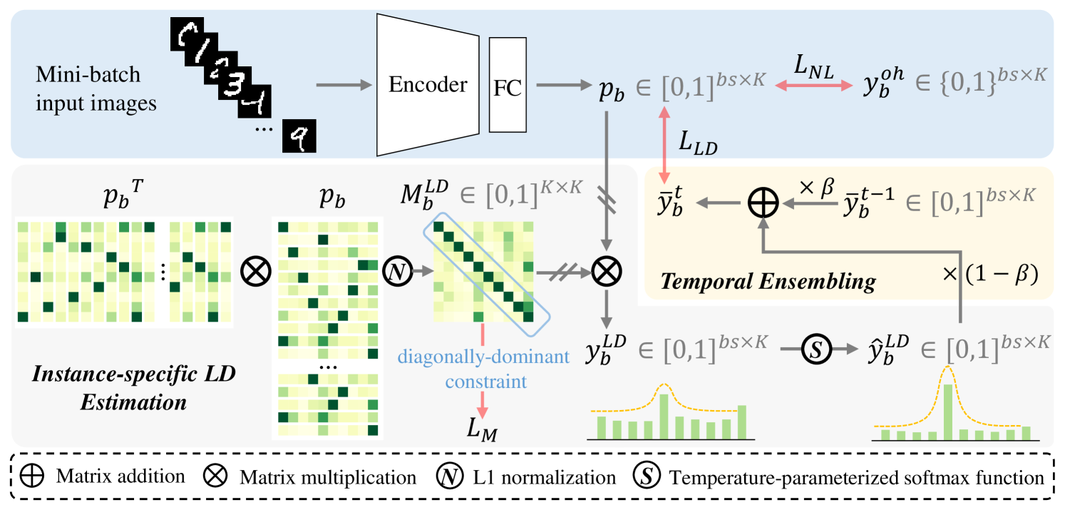
In this section, we dive into the details of the combination of cross-entropy (CE) loss and our LDR (see Fig. 1), and show how it works in a mini-batch.

4.1 Noisy Supervision

The latent useful information hidden in noisy labels is more or less ignored by statistically inconsistent methods. On the contrary, we learn all labels in the training set equally, whether the labels are correct or wrong. In a mini-batch, the images are input into an encoder followed by fully connected layers and a softmax function, and the batch-level prediction is denoted as $\textbf{p}_{b}\in[0,1]^{bs\times K}$, in which $bs$ is the number of samples in this mini-batch. Then we calculate the CE loss between the prediction $\textbf{p}_{b}$ and noisy labels as the noisy supervision, which is denoted as $L_{NL}$ and the formulation of $L_{NL}$ is

$$L_{NL}=-\frac{1}{bs}\sum_{i=1}^{bs}\textbf{y}_{b_{i}}^{oh}\log{\textbf{p}_{b_{i}}}$$ (2)

in which $\textbf{y}_{b_{i}}^{oh}$ is the one-hot encoding of $i$-th sample’s observed label in the mini-batch.

4.2 Label Distribution Supervision

In our LDR, we aim to estimate the instance-specific LD based on the estimated noise transition matrix and the estimated noisy posterior probabilities, and utilize instance-specific LD as supervision. The instance-specific LD is the clean posterior probabilities, which can be denoted as $\left[P\left(Y^{*}=k\mid\textbf{x}\right)\right]_{k=1}^{K}$, abbreviated to $P\left(Y^{*}\mid\textbf{x}\right)$. $P\left(Y^{*}\mid\textbf{x}\right)$ can be calculated by multiplying $P\left(Y^{*}\mid Y\right)$ and $P\left(Y\mid\textbf{x}\right)$. where $P\left(Y^{*}\mid Y\right)$ is the noise transition matrix, and $P\left(Y\mid\textbf{x}\right)$ is the noisy posterior probabilities. Due to the noisy supervision by noisy label $\textbf{y}_{b}^{oh}$ (see Eq. 2), the prediction $\textbf{p}_{b}$ is the estimation of the noisy posterior probabilities $P\left(Y\mid\textbf{x}\right)$. If the noise transition matrix $P\left(Y^{*}\mid Y\right)$ can be estimated, then the clean posterior probabilities $P\left(Y^{*}\mid\textbf{x}\right)$ is got.

A sample is more likely to be misassigned one of the similar class labels cohen2020separability ; beyer2020we . Hence the mislabeling probability is highly correlated with the inter-class correlation, which is treated as the noise transition matrix in this work. Specifically, the Gram Matrix, which has been widely used for spatial/channel/sample-wise correlations liu2020semi , is employed to represent the class-wise correlation. The batch-level noise transition matrix $M_{b}^{LD}\in[0,1]^{K\times K}$ is calculated by

$$M_{b}^{LD}=\mathcal{N}(\textbf{p}_{b}^{T}\times\textbf{p}_{b})$$ (3)

where $\mathcal{N}$ means the L1-normalization on each row of the column Gram matrix of prediction $\textbf{p}_{b}$. Now we have the estimation of $P\left(Y^{*}\mid Y\right)$ ($i.e.$, $M_{b}^{LD}$) and the estimation of $P\left(Y\mid\textbf{x}\right)$ ($i.e.$, $\textbf{p}_{b}$). Thus the estimated clean posterior probabilities $P\left(Y^{*}\mid\textbf{x}\right)$ ($i.e.$, the instance-specific LD) can be calculated as follow

$$\textbf{y}_{b}^{LD}=\textbf{p}_{b}\times M_{b}^{LD^{T}}$$ (4)

Note that we clip the gradient of $M_{b}^{LD}$ and $\textbf{p}_{b}$ before calculating the matrix multiplication between them.

Intuitively, the sharper LD labels can achieve better performance by reducing the impact of noise. Therefore, we utilize the temperature-parameterized softmax function to sharpen the estimated instance-specific LD ($i.e.$, $\textbf{y}_{b}^{LD}$). The temperature-parameterized softmax function can be formulated as follow

$$\sigma_{\tau}(\textbf{z})_{i}=\frac{\exp(z_{i}/\tau)}{\sum_{j}\exp(z_{j}/\tau)}$$ (5)

where z is the input vector, and $\tau$ is the temperature. When $0<\tau<1$, the input vector z can be sharpened; when $1<\tau$, the input vector z can be smoothed. So we set $\tau\in(0,1)$ for the proposed LDR.

We treat the running average of the sharpened instance-specific LD (denoted as $\hat{\textbf{y}}_{b}^{LD}$) as the target for each sample. In semi-supervised learning yang2022survey , this technique is known as temporal ensembling Laine2017TemporalEnsembling . The target vector of a mini-batch in $t$-th epoch is denoted as $\bar{\textbf{y}}_{b}^{t}$, which is calculated as follows

$$\bar{\textbf{y}}_{b}^{t}=\beta\times\bar{\textbf{y}}_{b}^{t-1}+(1-\beta)\times\hat{\textbf{y}}_{b}^{LD}$$ (6)

where $0\leq\beta<1$ is a hyper-parameter which means the momentum. Note that $\bar{\textbf{y}}_{b}^{0}$ is an all-zero tensor. We introduce $L_{LD}$ which maximizes the inner product between the prediction $\textbf{p}_{b}$ and the target $\bar{\textbf{y}}_{b}^{t}$. $L_{LD}$ can be formulated as

$$L_{LD}=-\frac{1}{bs}\sum_{i=1}^{bs}\log{(1-\bar{\textbf{y}}_{b_{i}}^{t}\textbf{p}_{b_{i}})}$$ (7)

Theoretically, CE loss and Kullback-Leibler divergence also can be utilized to push $\textbf{p}_{b}$ close to $\bar{\textbf{y}}_{b}^{t}$. However, the inner product is more effective and performs better liu2020early . Moreover, we introduce a diagonally-dominant constraint to make sure that $M_{b}^{LD}$ is diagonally-dominant. The corresponding regularization term $L_{M}$ is formulated as follow

$$L_{M}=\left\|M_{b}^{LD}\right\|_{2}^{2}-\left\|diag(M_{b}^{LD})\right\|_{2}^{2}$$ (8)

which represents the square of the L2 norm of all elements in the matrix $M_{b}^{LD}$ except the diagonal elements. The smaller $L_{M}$, the more dominant the diagonal of $M_{b}^{LD}$.

Figure 2: Training loss curves of CE+LDR on the CIFAR-10 dataset with asymmetric noise and noise rate is 0.5. (a,b,c,d) show the loss curves of $L_{NL}$, $L_{LD}$, $L_{M}$, and $L_{SUM}$, respectively.

4.3 Loss Function

The combination of CE loss and the proposed LDR is formulated as follows

$$L_{SUM}=L_{NL}+(\alpha\times L_{LD}+\delta\times L_{M})$$ (9)

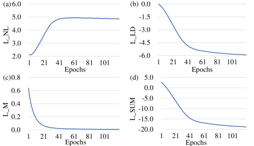
in which $\alpha$ and $\delta$ are the weighting hyper-parameters. It seems that $L_{NL}$ and $L_{LD}$ have conflicting optimization directions on noisy datasets. In fact, we set $\alpha>1.0$, so that the optimization focus on $L_{LD}$. And the value of $L_{NL}$ keeps getting bigger until convergence during training on noisy datasets (see Fig. 2). It is shown that LDR does not make the model blindly memorize the labels in the training set. However, the noisy supervision ($L_{NL}$) is essential for noise transition matrix estimation because noisy labels reflect inter-class correlation.

Table 1: Test accuracies (%, mean$\pm$standard deviation) of different methods on two datasets with clean or symmetric label noise ($\eta\in[0.2,0.4,0.6,0.8]$). The results are reported and the top two best results are highlighted with bold.

Dataset	Method	Clean	Symmetric Noise Rate
			0.2	0.4	0.6	0.8
MNIST	CE	99.08 $\pm$ 0.09	86.06 $\pm$ 0.76	66.70 $\pm$ 1.25	44.40 $\pm$ 1.66	20.89 $\pm$ 1.17
	SCE	99.01 $\pm$ 0.25	88.76 $\pm$ 0.49	69.04 $\pm$ 1.42	47.29 $\pm$ 0.62	21.19 $\pm$ 1.02
	ELR	99.18 $\pm$ 0.06	99.05 $\pm$ 0.06	98.87 $\pm$ 0.04	98.54 $\pm$ 0.12	91.37 $\pm$ 1.01
	AUL	99.18 $\pm$ 0.09	99.02 $\pm$ 0.05	98.88 $\pm$ 0.11	98.14 $\pm$ 0.20	97.14 $\pm$ 0.02
	AGCE	99.19 $\pm$ 0.07	99.05 $\pm$ 0.06	98.92 $\pm$ 0.07	98.36 $\pm$ 0.09	96.74 $\pm$ 0.15
	SR	99.30 $\pm$ 0.06	98.99 $\pm$ 0.10	98.93 $\pm$ 0.08	98.69 $\pm$ 0.12	98.37 $\pm$ 0.19
	GLS	99.33 $\pm$ 0.06	98.66 $\pm$ 0.06	97.94 $\pm$ 0.15	95.92 $\pm$ 0.31	76.65 $\pm$ 1.59
	VolMinNet	98.99 $\pm$ 0.13	98.87 $\pm$ 0.08	98.74 $\pm$ 0.09	98.46 $\pm$ 0.22	98.17 $\pm$ 0.19
	MEIDTM	99.04 $\pm$ 0.64	99.05 $\pm$ 0.37	98.95 $\pm$ 0.24	98.70 $\pm$ 0.32	98.35 $\pm$ 0.39
	Ours	99.18 $\pm$ 0.08	99.06 $\pm$ 0.09	98.95 $\pm$ 0.07	98.81 $\pm$ 0.07	98.39 $\pm$ 0.18
	Ours$*$	99.24 $\pm$ 0.07	99.14 $\pm$ 0.04	99.04 $\pm$ 0.04	98.84 $\pm$ 0.09	98.57 $\pm$ 0.04
CIFAR-10	CE	90.12 $\pm$ 0.17	71.87 $\pm$ 0.55	54.29 $\pm$ 1.23	36.43 $\pm$ 1.18	17.62 $\pm$ 0.32
	SCE	90.63 $\pm$ 0.26	77.01 $\pm$ 0.45	59.16 $\pm$ 0.97	40.23 $\pm$ 0.41	17.91 $\pm$ 0.32
	ELR	91.18 $\pm$ 0.28	88.68 $\pm$ 0.17	85.90 $\pm$ 0.17	77.04 $\pm$ 0.35	35.75 $\pm$ 1.42
	NCE+AUL	90.06 $\pm$ 0.11	88.06 $\pm$ 0.28	84.97 $\pm$ 0.21	77.95 $\pm$ 0.32	55.54 $\pm$ 1.59
	NCE+AGCE	89.82 $\pm$ 0.20	88.06 $\pm$ 0.20	84.67 $\pm$ 0.66	78.27 $\pm$ 0.77	47.55 $\pm$ 4.10
	SR	90.01 $\pm$ 0.06	88.04 $\pm$ 0.18	84.81 $\pm$ 0.16	78.02 $\pm$ 0.44	50.61 $\pm$ 0.93
	GLS	90.10 $\pm$ 0.36	81.99 $\pm$ 0.64	72.53 $\pm$ 0.71	61.80 $\pm$ 0.64	36.94 $\pm$ 1.88
	VolMinNet	89.92 $\pm$ 0.17	88.85 $\pm$ 0.29	85.99 $\pm$ 0.52	78.34 $\pm$ 0.56	54.37 $\pm$ 0.48
	MEIDTM	90.04 $\pm$ 0.46	89.01 $\pm$ 0.37	86.22 $\pm$ 0.68	78.51 $\pm$ 0.79	55.84 $\pm$ 0.95
	Ours	90.36 $\pm$ 0.16	89.35 $\pm$ 0.14	87.03 $\pm$ 0.41	79.34 $\pm$ 0.54	56.25 $\pm$ 0.82
	Ours$*$	90.92 $\pm$ 0.25	89.53 $\pm$ 0.12	87.27 $\pm$ 0.46	81.35 $\pm$ 0.43	59.10 $\pm$ 0.84

Table 2: Test accuracies (%, mean$\pm$standard deviation) of different methods on two datasets with asymmetric label noise ($\eta\in[0.1,0.2,0.3,0.4,0.5]$). The results are reported and the top two best results are highlighted with bold.

Dataset	Method	Asymmetric Noise Rate
		0.1	0.2	0.3	0.4	0.5
MNIST	CE	93.59 $\pm$ 0.59	86.74 $\pm$ 1.06	76.98 $\pm$ 0.99	66.28 $\pm$ 1.42	54.93 $\pm$ 1.88
	SCE	94.46 $\pm$ 0.29	88.50 $\pm$ 1.03	78.40 $\pm$ 1.28	69.19 $\pm$ 2.27	57.21 $\pm$ 1.49
	ELR	99.14 $\pm$ 0.07	99.00 $\pm$ 0.11	98.96 $\pm$ 0.09	98.79 $\pm$ 0.09	98.65 $\pm$ 0.10
	AUL	99.06 $\pm$ 0.03	99.04 $\pm$ 0.07	98.85 $\pm$ 0.16	98.87 $\pm$ 0.11	96.68 $\pm$ 3.78
	AGCE	99.10 $\pm$ 0.04	99.07 $\pm$ 0.04	98.87 $\pm$ 0.10	98.54 $\pm$ 0.22	97.57 $\pm$ 0.45
	SR	98.79 $\pm$ 0.05	98.99 $\pm$ 0.19	99.03 $\pm$ 0.06	98.96 $\pm$ 0.08	98.85 $\pm$ 0.10
	GLS	98.94 $\pm$ 0.06	98.71 $\pm$ 0.10	98.38 $\pm$ 0.09	97.56 $\pm$ 0.10	95.92 $\pm$ 0.65
	VolMinNet	99.03 $\pm$ 0.09	99.00 $\pm$ 0.15	98.95 $\pm$ 0.07	98.81 $\pm$ 0.07	98.77 $\pm$ 0.19
	MEIDTM	99.07 $\pm$ 0.32	99.04 $\pm$ 0.26	99.06 $\pm$ 0.12	98.85 $\pm$ 0.14	98.83 $\pm$ 0.21
	Ours	99.09 $\pm$ 0.07	99.09 $\pm$ 0.06	99.08 $\pm$ 0.06	98.98 $\pm$ 0.06	98.97 $\pm$ 0.06
	Ours$*$	99.20 $\pm$ 0.06	99.16 $\pm$ 0.08	99.10 $\pm$ 0.05	99.00 $\pm$ 0.08	98.97 $\pm$ 0.06
CIFAR-10	CE	80.97 $\pm$ 0.39	72.60 $\pm$ 0.98	63.24 $\pm$ 0.74	55.86 $\pm$ 0.82	46.81 $\pm$ 0.57
	SCE	82.89 $\pm$ 0.40	76.20 $\pm$ 0.51	67.82 $\pm$ 0.82	58.34 $\pm$ 0.76	49.60 $\pm$ 1.01
	ELR	89.11 $\pm$ 0.22	88.43 $\pm$ 0.26	87.17 $\pm$ 0.14	84.31 $\pm$ 0.64	75.00 $\pm$ 0.32
	NCE+AUL	88.76 $\pm$ 0.28	86.80 $\pm$ 0.57	85.38 $\pm$ 0.38	81.43 $\pm$ 0.60	74.68 $\pm$ 1.17
	NCE+AGCE	88.59 $\pm$ 0.23	86.97 $\pm$ 0.55	85.19 $\pm$ 0.35	81.03 $\pm$ 1.09	71.85 $\pm$ 0.58
	SR	88.89 $\pm$ 0.23	87.16 $\pm$ 0.15	85.25 $\pm$ 0.16	81.97 $\pm$ 0.18	76.58 $\pm$ 0.22
	GLS	84.60 $\pm$ 0.69	80.27 $\pm$ 0.63	76.40 $\pm$ 0.33	71.53 $\pm$ 0.87	65.07 $\pm$ 1.18
	VolMinNet	89.02 $\pm$ 0.41	87.56 $\pm$ 0.38	85.97 $\pm$ 0.46	83.87 $\pm$ 0.34	75.79 $\pm$ 0.63
	MEIDTM	89.18 $\pm$ 0.33	88.43 $\pm$ 0.27	87.26 $\pm$ 0.31	84.50 $\pm$ 0.40	77.23 $\pm$ 0.57
	Ours	89.83 $\pm$ 0.19	88.84 $\pm$ 0.30	88.03 $\pm$ 0.24	85.28 $\pm$ 0.46	77.88 $\pm$ 0.89
	Ours$*$	89.94 $\pm$ 0.18	89.20 $\pm$ 0.16	88.30 $\pm$ 0.23	85.89 $\pm$ 0.21	80.74 $\pm$ 0.51

5 Experiments

5.1 Experiment Setup

Synthetic Noisy Datasets The validation is constructed on two synthetic noisy datasets MNIST lecun1998gradient and CIFAR-10 krizhevsky2009learning . We consider two types of noisy labels for MNIST and CIFAR-10: (1) Symmetric noise: the GT label is corrupted randomly to any other class label; (2) Asymmetric noise: the GT label is corrupted to similar classes with higher probability. The two types of synthetic noise are class-dependent.

Real-world Noisy Datasets We also validate the effectiveness of LDR on two real-world noisy datasets CIFAR-10N and CIFAR-100N wei2021learning (jointly called CIFAR-N), which equipped the training datasets of CIFAR-10 and CIFAR-100 with human-annotated noisy labels collected from Amazon Mechanical Turk. CIFAR-10N provides five noisy label sets for training data, $i.e.$, Aggregate ($\eta$=$9.03\%$), Random 1 ($\eta$=$17.23\%$), Random 2 ($\eta$=$18.12\%$), Random 3 ($\eta$=$17.64\%$), and Worst ($\eta$=$40.21\%$). CIFAR-100N provides one noisy label set for training data ($\eta$=$40.20\%$). The human noise in CIFAR-N has been proven to be feature-dependent wei2021learning .

5.2 Implementation Details

For MNIST, we use two convolutional layers followed by two fully connected layers as the backbone. For CIFAR-10 and CIFAR-10N, six convolutional layers followed by two fully connected layers are utilized as the backbone. For CIFAR-100N, we use ResNet-34 he2016deep as the backbone. For all experiments, the SGD algorithm with a momentum of 0.9 is used as the optimizer, and the batch size is set to 128 consistently. The learning rate is set to 0.01 for MNIST, CIFAR-10, and CIFAR-10N, and 0.1 for CIFAR-100N. The weight decay is set to 1e-3, 1e-4, 1e-4, and 1e-5 for MNIST, CIFAR-10, CIFAR-10N, and CIFAR-100N, respectively. The model is trained for 50 epochs for MNIST, 120 epochs for CIFAR-10 and CIFAR-10N, and 200 epochs for CIFAR-100N. Random cropping and random horizontal flipping are adopted to increase the data diversity of CIFAR10, CIFAR-10N, and CIFAR-100N. All experiments were performed on a workstation with one NVIDIA 3080Ti GPU and implemented using the PyTorch framework. The experimental results are reported over five random runs.

5.3 Comparison with State-of-the-art Methods

We compare our LDR with seven state-of-the-art methods on two synthetic noisy datasets and two real-world noisy datasets: (1) Symmetric cross entropy (SCE) wang2019symmetric , which combines cross-entropy loss with reverse cross-entropy term; (2) Early-learning regularization (ELR) liu2020early , which utilizes the ensemble of historical predictions as supervision; (3) Asymmetric loss functions (AUL, AGCE, NCE+AUL, and NCE+AGCE) zhou2021asymmetric , which makes the optimization direction shift to the loss term of class with the maximum weight; (4) Sparse regularization (SR) zhou2021learning , which makes any loss be noise-robustness by restricting the prediction to the set of permutations over a fixed vector; (5) Generalized label smoothing (GLS) Wei2022ToSO , which uses the positively or negatively weighted average of both the hard observed labels and uniformly distributed soft labels as the target labels; (6) Volume Minimization Network (VolMinNet) li2021provably , which optimizes the trainable noise transition matrix by minimizing the volume of the simplex formed by the columns of the noise transition matrix; and (7) Manifold embedding instance-dependent transition matrix (MEIDTM) cheng2022instance , which proposes the practical assumption on the geometry of transition matrix to reduce the degree of freedom of transition matrix and make it stably estimable in practice. The baseline CE represents directly training a classification network with the standard cross-entropy loss on the noisy dataset. All competing methods are re-implemented using their released codes and the reported optimal hyper-parameters. The learning rate, batch size, weight decay, optimizer, epochs number, and backbone are kept the same for a fair comparison.

Results on Synthetic Noisy Datasets We compare LDR with other competing methods on MNIST and CIFAR-10 with symmetric (see Table 1) or asymmetric noise (see Table 2). All methods are compared on both datasets with a series of noise rates. Each competitor’s hyper-parameter setting under different noise rates is the same. However, the hyper-parameter of GLS is sensitive to noise rate, so we adjust the hyper-parameter of GLS under each noise rate case. Thus we provide ‘Ours’ and ‘Ours$*$’ in Table 1 and Table 2. ‘Ours’ means we use the same hyper-parameter setting under each noise rate case, while ‘Ours^∗’ means we use different hyper-parameter settings under each noise rate case.

Although GLS and ELR perform better on the clean set of MNIST (GLS: 99.33% v.s. Ours^∗: 99.24%) and CIFAR-10 (ELR: 91.18% v.s. Ours^∗: 90.92%), our LDR achieves the best result on all symmetric noisy cases and most asymmetric noisy cases. Moreover, our LDR outperforms other competing methods in the most difficult situations by a clear margin. On CIFAR-10 with symmetric noise ($\eta$=0.8), LDR outperforms the best competitor MEIDTM by 3.26% (59.10% v.s. 55.84%; p-value=4.54e-4$<$0.05). On CIFAR-10 with asymmetric noise ($\eta$=0.5), our LDR outperforms the best competitor MEIDTM by 3.51% (80.74% v.s. 77.23%; p-value=7.65e-6$<$0.05). In addition, although our gain on symmetric/asymmetric noisy MNIST is only 0.2%/0.12% (p-value=0.077/0.057), we achieve an average accuracy of 98.57%/98.97%, which we believe is saturated on MNIST.

Table 3: Comparison of test accuracies (%, mean$\pm$standard deviation) on CIFAR-10N and CIFAR-100N using different methods. The top two results are highlighted with bold.

Method	CIFAR-10N					CIFAR-100N
	Aggregate	Random 1	Random 2	Random 3	Worst	Noisy
CE	84.05 $\pm$ 0.20	77.15 $\pm$ 0.76	76.07 $\pm$ 0.73	76.96 $\pm$ 0.65	59.10 $\pm$ 0.25	44.49 $\pm$ 1.40
SCE	84.98 $\pm$ 0.29	78.96 $\pm$ 0.44	78.59 $\pm$ 0.59	79.02 $\pm$ 0.48	62.60 $\pm$ 0.86	45.42 $\pm$ 1.49
ELR	88.53 $\pm$ 0.47	87.35 $\pm$ 0.27	87.49 $\pm$ 0.49	87.12 $\pm$ 0.19	81.19 $\pm$ 0.61	45.48 $\pm$ 0.59
NCE+AUL	88.13 $\pm$ 0.43	86.28 $\pm$ 0.50	86.28 $\pm$ 0.68	86.54 $\pm$ 0.29	78.82 $\pm$ 0.73	52.01 $\pm$ 0.83
NCE+AGCE	87.84 $\pm$ 0.16	86.51 $\pm$ 0.32	86.61 $\pm$ 0.25	86.20 $\pm$ 0.52	78.56 $\pm$ 0.89	54.82 $\pm$ 0.48
SR	88.38 $\pm$ 0.23	87.18 $\pm$ 0.18	86.95 $\pm$ 0.20	87.04 $\pm$ 0.18	79.51 $\pm$ 0.34	52.45 $\pm$ 0.30
GLS	84.93 $\pm$ 0.44	81.93 $\pm$ 0.45	81.83 $\pm$ 0.53	81.77 $\pm$ 0.48	72.86 $\pm$ 1.12	46.97 $\pm$ 0.94
VolMinNet	88.83 $\pm$ 0.22	87.30 $\pm$ 0.14	87.14 $\pm$ 0.17	87.01 $\pm$ 0.25	80.07 $\pm$ 0.47	54.69 $\pm$ 0.46
MEIDTM	89.10 $\pm$ 0.24	87.89 $\pm$ 0.12	87.93 $\pm$ 0.17	87.54 $\pm$ 0.21	81.43 $\pm$ 0.30	55.06 $\pm$ 0.41
Ours	89.16 $\pm$ 0.15	88.52 $\pm$ 0.60	88.52 $\pm$ 0.15	88.19 $\pm$ 0.57	82.74 $\pm$ 0.69	55.95 $\pm$ 0.47
Ours*	89.49 $\pm$ 0.16	88.52 $\pm$ 0.60	88.55 $\pm$ 0.19	88.52 $\pm$ 0.15	82.74 $\pm$ 0.69	57.83 + 0.61

Results on Real-world Noisy Datasets We evaluate our LDR and other competitors on two real-world noisy datasets, CIFAR-10N and CIFAR-100N, which are human-annotated, and the results are shown in Table 3. In Table 3, except for GLS and Ours^∗, other methods use the same hyper-parameters setting for all noisy label sets on each dataset. As shown in 3, under the feature-dependent noise which is more challenging than synthetic label noise, our LDR also outperforms the best-competitor by 2.77%/1.31% on CIFAR-100N/CIFAR-10N-Worst (p-value=6.52e-5/9.68e-3$<$0.05), The results demonstrate that the proposed LDR can help the trained classifier against real-world label noise.

5.4 Ablation studies

We conducted ablation studies on CIFAR-10 with asymmetric noise (noise rate is 0.5) to investigate the effectiveness of $L_{LD}$ and $L_{M}$ of LDR, respectively. We validate CE+LDR and its two variants in Table 4. ‘$L_{NL}$’ means only using the CE loss between the predictions and noisy labels, ‘$L_{NL}+L_{LD}$’ means using CE+LDR without diagonally-dominant constraint $L_{M}$, and ‘$L_{NL}+L_{LD}+L_{M}$ means the complete CE+LDR. When $L_{LD}$ and $L_{M}$ were removed, the performance drops seriously.

Moreover, there are two important operations in $L_{LD}$ of LDR, $i.e.$, the estimated instance-specific LD sharpening (Eq. 5) and temporal ensembling (Eq. 6). We conducted experiments on CIFAR-10 to validate their effectiveness. Table 5 gives the performance of the CE+LDR with complete $L_{LD}$ and its two variants. When sharpening or temporal ensembling is removed, the performance is more or less degraded.

Table 4: Test accuracy (%, mean$\pm$standard deviation) of CE+LDR and its variants on CIFAR-10 with asymmetric noise ($\eta$=0.5). The best result is highlighted with bold.

$L_{NL}$	$L_{LD}$	$L_{M}$	Accuracy
$\checkmark$			46.81 $\pm$ 0.57
$\checkmark$	$\checkmark$		70.19 $\pm$ 0.56
$\checkmark$	$\checkmark$	$\checkmark$	80.74 $\pm$ 0.51

6 Discussions

6.1 Hyper-parameter Settings

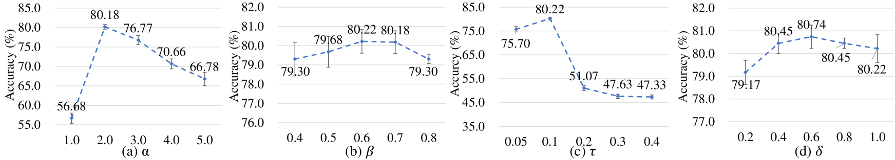
In the proposed LDR, there are four hyper-parameters that should be adjusted, $i.e.$, the weighting factors $\alpha$ and $\delta$ in the loss function (Eq. 9), the weighting factor $\beta$ in temporal ensembling (Eq. 6), and the sharpen factor $\tau$ in Eq. 5. We show the hyper-parameters adjustment experiments on CIFAR-10 with an asymmetric noise rate of 0.5 in Fig. 3. We set $\alpha=2.0,\beta=0.7,\tau=0.1,\delta=1.0$ for initialization and adjust these four hyper-parameters one by one. Note that we adjust the value of one hyper-parameter while fixing the other three. Finally these hyper-parameters are set as $\alpha=2.0,\beta=0.6,\tau=0.1,\delta=0.6$ for CIFAR-10 with asymmetric noise rate ($\eta$=0.5).

Figure 3: Test Accuracy (%) of CE+LDR trained on CIFAR-10 (asymmetric noise rate is 0.5) with different hyper-parameters settings. (a,b,c,d) show the performances of LDR with different values of $\alpha$, $\beta$, $\tau$ and $\delta$, respectively. The mean and standard deviation of five runs’ performances are shown here.

Table 5: Test accuracy (%, mean$\pm$standard deviation) of CE+LDR with complete $L_{LD}$ and its variants on the CIFAR-10 dataset with asymmetric noise ($\eta$=0.5). The best result is highlighted with bold.

Temporal Ensembling	Sharpening	Accuracy
		75.85 $\pm$ 0.60
$\checkmark$		79.71 $\pm$ 0.30
$\checkmark$	$\checkmark$	80.74 $\pm$ 0.51

6.2 Analysis of Batch Size

The noise transition matrix estimation is essential to the estimation of instance-specific label distribution. In LDR, we estimate the noise transition matrix by Eq. 3, in which the batch size directly affects the estimation results. Thus we want to explore how the batch size affects the performance of our LDR. We conducted experiments on CIFAR-10 with an asymmetric noise rate of 0.5, and the hyper-parameters in LDR are set to $\alpha=2.0,\beta=0.6,\tau=0.1,\delta=0.6$. Under this case, different batch sizes are tried to perform and the results are shown in Table 6. When the batch size drops from 128 to 32, the performance of LDR is further improved (80.74% v.s. 84.43%). As can be seen, the smaller the batch size is, the more the estimated noise transition matrix is suitable for each sample in the mini-batch. However, as the batch size continues to degrade, the performance of LDR deteriorates. That is because a small number of samples are difficult to reflect the real inter-class correlation.

Table 6: Test accuracies (%, mean$\pm$standard deviation) of CE+LDR trained on CIFAR-10 (asymmetric noise rate is 0.5) with different batch sizes. The best result is highlighted with bold.

Batch Size	Test Accuracy
128	80.74 $\pm$ 0.51
64	82.74 $\pm$ 0.55
32	84.43 $\pm$ 0.43
16	83.33 $\pm$ 0.65
8	78.83 $\pm$ 0.69

6.3 Memorization of Noisy Training Data

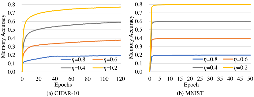
We visualize the memory accuracy curves of the proposed LDR trained on the synthetic noisy datasets MNIST and CIFAR-10, whose symmetric noise rates are set to $[0.2,0.4,0.6,0.8]$, respectively, as shown in Fig. 4. The memory accuracy is calculated between the predictions for training samples and the noisy labels of training data. It is expected that the classifier memorizes all training samples with clean labels, and does not memorize that with noisy labels. As shown in Fig. 4, when the noise rate is set to 0.8, which is the hardest case, both memory accuracy curves of the two datasets converge to 0.2, indicating that the proposed LDR can effectively prevent the classifier from memorizing noisy labels.

Figure 4: Memory accuracy of classifiers trained on MNIST and CIFAR-10 datasets with symmetric noise ($\eta\in[0.2,0.4,0.6,0.8]$). Memory accuracy is calculated between training samples’ observed labels and the prediction of the classifier.

6.4 Training time cost

Table 7 shows the training time cost of all competing methods on the CIFAR-10N dataset. It shows that the training time of our LDR is comparable with that of CE, SCE, VolMinNet, MEIDTM, and GLS. But the accuracy of LDR is better (see Table 3).

Table 7: Training time cost of all competing methods on the CIFAR-10N dataset.

Method	Training Time Cost
CE	18min17s
SCE	18min36s
ELR	19min19s
NCE+AUL	19min33s
NCE+AGCE	19min32s
SR	20min07s
GLS	18min48s
VolMinNet	18min45s
MEIDTM	18min09s
Our LDR	18min39s

7 Conclusion

In this paper, we propose an instance-specific Label Distribution Regularization (LDR) method, in which the instance-specific LD is estimated as supervision, to prevent DCNNs from memorizing noisy labels. In contrast to existing noise transition matrix methods, we propose to approximate the noise transition matrix by estimating the inter-class correlation matrix without either anchor points or pseudo anchor points. Moreover, our estimation of the noise transition matrix, which does not require an extra training stage, is more efficient than most existing methods. Ablation study shows the effectiveness of modeling batch-level noise transition matrix. And experimental results on two synthetic noisy datasets and two real-world noisy datasets demonstrate the proposed LDR outperforms other competitors.

References

- \bibcommenthead
- (1) Yu, X., Liu, T., Gong, M., Tao, D.: Learning with biased complementary labels. In: Proceedings of the European Conference on Computer Vision, pp. 68–83 (2018)
- (2) Zhang, C., Bengio, S., Hardt, M., Recht, B., Vinyals, O.: Understanding deep learning requires rethinking generalization. International Conference on Learning Representations (2017)
- (3) Han, B., Yao, Q., Yu, X., Niu, G., Xu, M., Hu, W., Tsang, I., Sugiyama, M.: Co-teaching: Robust training of deep neural networks with extremely noisy labels. Advances in Neural Information Processing Systems 31 (2018)
- (4) Li, J., Socher, R., Hoi, S.C.: Dividemix: Learning with noisy labels as semi-supervised learning. In: International Conference on Learning Representations (2019)
- (5) Wang, Y., Sun, X., Fu, Y.: Scalable penalized regression for noise detection in learning with noisy labels. In: Proceedings of the IEEE/CVF Conference on Computer Vision and Pattern Recognition, pp. 346–355 (2022)
- (6) Xia, X., Liu, T., Han, B., Gong, C., Wang, N., Ge, Z., Chang, Y.: Robust early-learning: Hindering the memorization of noisy labels. In: International Conference on Learning Representations (2020)
- (7) Kim, Y., Yim, J., Yun, J., Kim, J.: Nlnl: Negative learning for noisy labels. In: Proceedings of the IEEE/CVF International Conference on Computer Vision, pp. 101–110 (2019)
- (8) Thulasidasan, S., Bhattacharya, T., Bilmes, J.A., Chennupati, G., Mohd-Yusof, J.: Combating label noise in deep learning using abstention. In: International Conference on Machine Learning (2019)
- (9) Patrini, G., Rozza, A., Krishna Menon, A., Nock, R., Qu, L.: Making deep neural networks robust to label noise: A loss correction approach. In: Proceedings of the IEEE/CVF Conference on Computer Vision and Pattern Recognition, pp. 1944–1952 (2017)
- (10) Xia, X., Liu, T., Han, B., Gong, M., Yu, J., Niu, G., Sugiyama, M.: Sample selection with uncertainty of losses for learning with noisy labels. International Conference on Learning Representations (2022)
- (11) Huang, Y., Bai, B., Zhao, S., Bai, K., Wang, F.: Uncertainty-aware learning against label noise on imbalanced datasets. Proceedings of the AAAI Conference on Artificial Intelligence (2022)
- (12) Li, X., Liu, T., Han, B., Niu, G., Sugiyama, M.: Provably end-to-end label-noise learning without anchor points. In: International Conference on Machine Learning, pp. 6403–6413 (2021). PMLR
- (13) Cheng, D., Liu, T., Ning, Y., Wang, N., Han, B., Niu, G., Gao, X., Sugiyama, M.: Instance-dependent label-noise learning with manifold-regularized transition matrix estimation. In: Proceedings of the IEEE/CVF Conference on Computer Vision and Pattern Recognition, pp. 16630–16639 (2022)
- (14) Hendrycks, D., Mazeika, M., Wilson, D., Gimpel, K.: Using trusted data to train deep networks on labels corrupted by severe noise. Advances in neural information processing systems 31 (2018)
- (15) Xia, X., Liu, T., Wang, N., Han, B., Gong, C., Niu, G., Sugiyama, M.: Are anchor points really indispensable in label-noise learning? Advances in Neural Information Processing Systems 32 (2019)
- (16) Shu, J., Zhao, Q., Xu, Z., Meng, D.: Meta transition adaptation for robust deep learning with noisy labels. arXiv preprint arXiv:2006.05697 (2020)
- (17) Yao, Y., Liu, T., Han, B., Gong, M., Deng, J., Niu, G., Sugiyama, M.: Dual t: Reducing estimation error for transition matrix in label-noise learning. Advances in neural information processing systems 33, 7260–7271 (2020)
- (18) Cheng, H., Zhu, Z., Li, X., Gong, Y., Sun, X., Liu, Y.: Learning with instance-dependent label noise: A sample sieve approach. In: International Conference on Learning Representations (2020)
- (19) Berthon, A., Han, B., Niu, G., Liu, T., Sugiyama, M.: Confidence scores make instance-dependent label-noise learning possible. In: International Conference on Machine Learning, pp. 825–836 (2021). PMLR
- (20) Xia, X., Liu, T., Han, B., Wang, N., Gong, M., Liu, H., Niu, G., Tao, D., Sugiyama, M.: Part-dependent label noise: Towards instance-dependent label noise. Advances in Neural Information Processing Systems 33, 7597–7610 (2020)
- (21) Yang, S., Yang, E., Han, B., Liu, Y., Xu, M., Niu, G., Liu, T.: Estimating instance-dependent label-noise transition matrix using dnns. arXiv preprint arXiv:2105.13001 (2021)
- (22) Zhou, X., Liu, X., Jiang, J., Gao, X., Ji, X.: Asymmetric loss functions for learning with noisy labels. In: International Conference on Machine Learning, pp. 12846–12856 (2021)
- (23) Cohen, U., Chung, S., Lee, D.D., Sompolinsky, H.: Separability and geometry of object manifolds in deep neural networks. Nature Communications 11(1), 1–13 (2020)
- (24) Beyer, L., Hénaff, O.J., Kolesnikov, A., Zhai, X., Oord, A.v.d.: Are we done with imagenet? arXiv preprint arXiv:2006.07159 (2020)
- (25) Gatys, L., Ecker, A., Bethge, M.: A neural algorithm of artistic style. Journal of Vision 16(12), 326–326 (2016)
- (26) Liu, S., Niles-Weed, J., Razavian, N., Fernandez-Granda, C.: Early-learning regularization prevents memorization of noisy labels. Advances in Neural Information Processing Systems 33, 20331–20342 (2020)
- (27) Laine, S., Aila, T.: Temporal ensembling for semi-supervised learning. In: International Conference on Learning Representations (2017)
- (28) Nguyen, D.T., Mummadi, C.K., Ngo, T.P.N., Nguyen, T.H.P., Beggel, L., Brox, T.: Self: Learning to filter noisy labels with self-ensembling. In: International Conference on Learning Representations (2019)
- (29) Jiang, L., Zhou, Z., Leung, T., Li, L.-J., Fei-Fei, L.: Mentornet: Learning data-driven curriculum for very deep neural networks on corrupted labels. In: International Conference on Machine Learning, pp. 2304–2313 (2018)
- (30) Wei, J., Liu, H., Liu, T., Niu, G., Liu, Y.: To smooth or not? when label smoothing meets noisy labels. In: International Conference on Machine Learning (2022)
- (31) Ghosh, A., Kumar, H., Sastry, P.S.: Robust loss functions under label noise for deep neural networks. In: Proceedings of the AAAI Conference on Artificial Intelligence, vol. 31 (2017)
- (32) Zhang, Z., Sabuncu, M.: Generalized cross entropy loss for training deep neural networks with noisy labels. Advances in Neural Information Processing Systems 31 (2018)
- (33) Wang, Y., Ma, X., Chen, Z., Luo, Y., Yi, J., Bailey, J.: Symmetric cross entropy for robust learning with noisy labels. In: Proceedings of the IEEE/CVF International Conference on Computer Vision, pp. 322–330 (2019)
- (34) Lyu, Y., Tsang, I.W.: Curriculum loss: Robust learning and generalization against label corruption. International Conference on Learning Representations (2019)
- (35) Ma, X., Huang, H., Wang, Y., Romano, S., Erfani, S., Bailey, J.: Normalized loss functions for deep learning with noisy labels. In: International Conference on Machine Learning, pp. 6543–6553 (2020)
- (36) Yao, Y., Deng, J., Chen, X., Gong, C., Wu, J., Yang, J.: Deep discriminative cnn with temporal ensembling for ambiguously-labeled image classification. In: Proceedings of the AAAI Conference on Artificial Intelligence, vol. 34, pp. 12669–12676 (2020)
- (37) Menon, A.K., Rawat, A.S., Reddi, S.J., Kumar, S.: Can gradient clipping mitigate label noise? In: International Conference on Learning Representations (2019)
- (38) Zhou, X., Liu, X., Wang, C., Zhai, D., Jiang, J., Ji, X.: Learning with noisy labels via sparse regularization. In: Proceedings of the IEEE/CVF International Conference on Computer Vision, pp. 72–81 (2021)
- (39) Natarajan, N., Dhillon, I.S., Ravikumar, P.K., Tewari, A.: Learning with noisy labels. Advances in neural information processing systems 26 (2013)
- (40) Yu, X., Liu, T., Gong, M., Batmanghelich, K., Tao, D.: An efficient and provable approach for mixture proportion estimation using linear independence assumption. In: Proceedings of the IEEE Conference on Computer Vision and Pattern Recognition, pp. 4480–4489 (2018)
- (41) Yao, Y., Liu, T., Han, B., Gong, M., Niu, G., Sugiyama, M., Tao, D.: Towards mixture proportion estimation without irreducibility. arXiv preprint arXiv:2002.03673 (2020)
- (42) Wei, J., Zhu, Z., Cheng, H., Liu, T., Niu, G., Liu, Y.: Learning with noisy labels revisited: A study using real-world human annotations. In: International Conference on Learning Representations (2021)
- (43) Liu, Q., Yu, L., Luo, L., Dou, Q., Heng, P.A.: Semi-supervised medical image classification with relation-driven self-ensembling model. IEEE transactions on medical imaging 39(11), 3429–3440 (2020)
- (44) Yang, X., Song, Z., King, I., Xu, Z.: A survey on deep semi-supervised learning. IEEE Transactions on Knowledge and Data Engineering (2022)
- (45) LeCun, Y., Bottou, L., Bengio, Y., Haffner, P.: Gradient-based learning applied to document recognition. Proceedings of the IEEE 86(11), 2278–2324 (1998)
- (46) Krizhevsky, A., Hinton, G., et al.: Learning multiple layers of features from tiny images (2009)
- (47) He, K., Zhang, X., Ren, S., Sun, J.: Deep residual learning for image recognition. In: Proceedings of the IEEE/CVF Conference on Computer Vision and Pattern Recognition, pp. 770–778 (2016)