Quaternion Tensor Completion with Sparseness for Color Video Recovery

Abstract

A novel low-rank completion algorithm based on the quaternion tensor is proposed in this paper. This approach uses the TQt-rank of quaternion tensor to maintain the structure of RGB channels throughout the entire process. In more detail, the pixels in each frame are encoded on three imaginary parts of a quaternion as an element in a quaternion matrix. Each quaternion matrix is then stacked into a quaternion tensor. A logarithmic function and truncated nuclear norm are employed to characterize the rank of the quaternion tensor in order to promote the low rankness of the tensor. Moreover, by introducing a newly defined quaternion tensor discrete cosine transform-based (QTDCT) regularization to the low-rank approximation framework, the optimized recovery results can be obtained in the local details of color videos. In particular, the sparsity of the quaternion tensor is reasonably characterized by $l_{1}$ norm in the QDCT domain. This strategy is optimized via the two-step alternating direction method of multipliers (ADMM) framework. Numerical experimental results for recovering color videos show the obvious advantage of the proposed method over other potential competing approaches.

I Introduction

WITH the development of computer vision processing, the effective recovery of missing color videos has become an indispensable research direction because high-dimensional images would inevitably be damaged; for instance, because of a bad imaging environment or poor transfer process. The main task of color video restoration is to recover missing elements in incomplete color video from limited observation. As a kind of high-dimensional data, color videos can be naturally represented by tensors because tensors are high-dimensional vectors, which are the generalization of matrices and vectors. Based on tensor representation, color video restoration can be transformed into a tensor completion (TC) problem, and the key to this issue is to ascertain the correlation between observed and missing elements [1].

Like matrix completion, comprehensive research has been conducted on low-rank based models, resulting in numerous improvements. Concretely, high-dimensional visual data has many similar and repeating patterns, thus, the image or video data has a highly correlated underlying structure [2]. In this way, the main task of low-rank TC (LRTC) is to build a low-rank regularization as per the previous description of the association between the observed and missing elements, enabling the filling of missing elements.

Unlike matrix-based methods, which need to pull high-dimensional data into vectors or matrices for processing, tensor can maintain the high-dimensional structure of the data itself. For example, a color image (with red, green, and blue channels) can be regarded as a third-order tensor, and a color video consisting of frame-by-frame color images can be considered as a fourth-order tensor similarly. Furthermore, unlike the uniqueness of the definition of the rank of a matrix, the definition of the rank of a tensor is not unique, e.g., the CANDECOMP/PARAFAC (CP) rank [3, 4] , the Tucker rank [5] and the tubal rank that in the light of tensor singular value decomposition (t-SVD) [6, 7, 8], etc.

The CP rank and the Tucker rank are the two most commonly utilized tensor ranks. The CP rank is defined as the minimum number of rank-1 tensors used to express a tensor by tallying this series of rank-1 tensors. It can be observed that although the CP rank is consistent with the definition of rank of matrix, it is difficult to identify a replaceable form that can be solved [9]. Hence, many CP-based methods directly utilize CP decomposition to characterize low-rankness of high-dimensional visual data [3]. The Tucker rank is defined as a vector, the k-th element in the vector is the rank of the mode-k unfolding of the tensor that is an unfolding matrix [10]. Inspired by the success of nuclear norm (NN) as the tightest convex surrogate of the matrix rank, methods based on Tucker rank generally adopt the sum of NN (SNN) of all the unfolding matrices of the tensor. Consequently, the problem evolves to how to optimize the SNN to achieve low-rank characterization. To avoid all singular values being treated equally, the method of adding weights to the NN of unfolding matrices was proposed in [1]. The weighted method entails introducing additional parameters, which weakens the degree of robustness. To overcome this disadvantage, the logarithm of singular values was designed, which allows larger singular values to be given smaller weights, because larger singular values carry more important information [11]. Although SNN can effectively apply the relationship among different modes after unfolding, the structure of high-dimensional data is inevitably destroyed during the process of unfolding a tensor to a matrix along one mode.

Moreover, based on t-SVD, the tubal rank also has been extensively studied in recent years. The definition of t-SVD was suggested in [7], then based on the novel definition of tensor-tensor product and some properties of t-SVD that are similar to SVD, the definition of the tubal nuclear norm was put forward [6]. This norm was defined by the sum of NN of all slices of tensor in the Fourier domain. Furthermore, in [8], the tensor truncated nuclear norm (T-TNN) was proposed for a superior estimation of rank since the larger the singular value, the less it will affect the rank. In addition, in [12], inspired by a novel tensor-tensor product defined in [13], a more general tensor NN was proposed induced by linear transforms such as Discrete Cosine Transform (DCT) and Random Orthogonal Matrix (ROM), etc. Approaches based on the tubal NN have proven to be effective in practical application by preserving the intrinsic structure of a tensor [14, 15]. However, the definition of t-SVD is designed for third-order tensors, so when dealing with color videos, this type of method needs to perform dimensional reduction operations, which also means that the structure among RGB will be disregarded. To overcome the above issue, in this paper, a color video is represented by a third order quaternion tensor as the pixel values of RGB channels can be placed in three imaginary parts of a quaternion. In fact, the quaternion-based strategies were proposed to process high-dimensional visual data and outstanding results were returned, e.g., color face recognition [16], color image and video completion [17], classification of biomedical color image [18], etc. In most of the quaternion-based methods, a color image is regarded as a quaternion matrix. In order to extend the definition of quaternion matrix and fully preserve the structure of color channels, in [17], the concept of quaternion tensor is presented. More specifically, a color image and a color video can be reconstructed as a two-dimensional quaternion tensor and a three- dimensional quaternion tensor, respectively. Considering the definition of quaternion tensor, in this paper, a color video is put in a three- dimensional quaternion tensor, and the visible explanation of a three- dimensional quaternion tensor representing a color video can be seen in Fig.1.

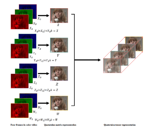
Figure 1: The illustration of a color video is represented by a three-dimensional quaternion tensor, taking four frames as an example.

As shown in Fig.1, it is expected to extend the t-SVD to the quaternion domain such that the color information and spatial structure of a video are preserved to the greatest extent. Not only that, inspired by the novel transform-based tensor product and corresponding transform-based quaternion tensor SVD (TQt-SVD) defined in the quaternion domain in [19], a TQt-SVD based on Quaternion Discrete Cosine Transform (QDCT) is adopted to address the low-rank recovery problem in this paper. Furthermore, to more accurately depict the low-rankness, the proposed model encompasses a truncated strategy and logarithmic function of singular values.

Not limited to the low-rank property, due to the fact that some signals in real visual data, such as audio, color images, and videos, can be represented sparsely by fixed bases [20], the sparse property of a color video can be found in some transformed domain. Thus, many methods previously considered sparseness by formulating it as a $l_{1}$ norm regularizer in a specific domain [21, 22].

Considering the above, this paper develops a novel quaternion tensor recovery model, which accounts for both the low-rankness and sparseness of the underlying quaternion tensor. The detailed demonstration of this regularization can be found in Section III.

The main contribution of this paper is summarized as follows:

• This work concentrate on quaternion tensor recovery, and a novel quaternion tensor completion model is developed, which simultaneously depicts the low rankness and the sparseness of the target quaternion tensor. The color visual data is addressed in the quaternion domain, which prevents corruption of the data structures.

• The low-rankness is depicted by introducing a truncated strategy and logarithmic function to the singular value for a more accurate substitute of the rank function, which is based on TQt-SVD.

• There is no decrease in dimensionality or slicing of the quaternion tensor, and the sparse regularization of the target quaternion tensor is designed, which is based on the quaternion tensor DCT (QTDCT) defined in this paper.

• This model alternates between the two steps with ADMM so as to optimize its development. The simulations on color videos recovery demonstrate that the proposed method outperforms state-of-the-art and comparable tensor-based and quaternion tensor-based methods.

The rest of this paper is arranged as follows. Section II presents some notations preliminaries used in this paper. Section III is devoted to introduce the proposed low-rank approximation and the sparse regularization. Section IV gives the corresponding recovery models and two-step optimization with ADMM. Section V then provides the numerical results to show the efficiency of the proposed method, while Section VI offers a conclusion to the work.

II Notations and Preliminaries

II-A Notations

In the real domain $\mathbb{R}$, scalar, vector, matrix, and tensor are denoted as a, $\mathbf{a}$, $\mathbf{A}$, and $\mathcal{A}$, respectively. In the quaternion domain $\mathbb{H}$, scalar, vector, matrix, and tensor are denoted as $\dot{a}$, $\dot{\mathbf{a}}$, $\dot{\mathbf{A}}$, and $\dot{\mathcal{A}}$, respectively. Besides, the complex space is denoted as $\mathbb{C}$. For a quaternion $\dot{q}$, the real part and imaginary part are denoted as $\mathfrak{R}(\dot{q})$ and $\mathfrak{I}(\dot{q})$. For a quaternion tensor $\dot{\mathcal{A}}\in\mathbb{H}^{I_{1}\times I_{2}\times\cdots\times I_{N}}$, the frontal slice is denoted by the Matlab notation $\dot{\mathcal{A}}(:,:,i_{3},\cdots,i_{N})$, where $i_{k}=1,\cdots,I_{k},$ for $k=3,\cdots,N$. Compactly, $\dot{\mathcal{A}}(:,:,i_{3},\cdots,i_{N})$ is denoted by $\dot{\mathcal{A}}^{(k)}$. The transpose, conjugate transpose, and inverse are denoted as $\mathbf{(\cdot)}^{T}$, $\mathbf{(\cdot)}^{H}$, and $\mathbf{(\cdot)}^{-1}$, respectively. The inner product of $*_{1}$ and $*_{2}$ is defined as $\langle*_{1}\cdot*_{2}\rangle\triangleq\text{tr}(*_{1}^{H}*_{2})$, where $tr(\cdot)$ is the trace function. The $\times_{k}$ represents the $k$-mode product. The trace function of $\dot{\mathcal{A}}$ is defined as $tr(\dot{\mathcal{A}})=\sum_{i=1}^{I_{3}}tr(\dot{\mathcal{A}}^{(i)}).$ $\mathbf{I}$ denotes the identity matrix.

II-B Preliminaries

II-B1 Quaternion basics

As an extension of complex numbers, quaternions are discovered by Hamilton in 1843 [23]. A quaternion number $\dot{q}\in\mathbb{H}$ can be represented as

$$\dot{q}=q_{0}+q_{1}\emph{i}+q_{2}\emph{j}+q_{3}\emph{k},$$

where $q_{n}\in\mathbb{R}$ $(n=0,1,2,3)$, and i, j, k are imaginary units which have the following relations:

$$\begin{cases}\emph{i}^{2}=\emph{j}^{2}=\emph{k}^{2}=\emph{i}\emph{j}\emph{k}=-1\\ \emph{i}\emph{j}=-\emph{j}\emph{i}=\emph{k},\emph{j}\emph{k}=-\emph{k}\emph{j}=\emph{i},\emph{k}\emph{i}=-\emph{i}\emph{k}=\emph{j}.\end{cases}$$

Let $\dot{q}=\mathfrak{R}(\dot{q})+\mathfrak{I}(\dot{q})$, where $\mathfrak{R}(\dot{q})\triangleq q_{0}$ is the real part of $\dot{q}$, and $\mathfrak{I}(\dot{q})\triangleq q_{1}\emph{i}+q_{2}\emph{j}+q_{3}\emph{k}$ is the imaginary part of $\dot{q}$. If real part $q_{0}=0$, $\dot{q}$ is a pure quaternion. A quaternion can be denoted by the Cayley-Dickson notation: $\dot{q}=\alpha+\beta j$, where $\alpha=a+bi$ and $\beta=c+di\in\mathbb{C}$. The conjugate and the modulus of $\dot{q}$ are formulated as $\dot{q}^{*}\triangleq q_{0}-q_{1}\emph{i}-q_{2}\emph{j}-q_{3}\emph{k}$ and $|\dot{q}|\triangleq\sqrt{\dot{q}\dot{q}^{*}}=\sqrt{q_{0}^{2}+q_{1}^{2}+q_{2}^{2}+q_{3}^{2}}$, respectively. Given two quaternions $\dot{p}$ and $\dot{q}\in\mathbb{H}$, the addition and multiplication are separately formulated as

$$\dot{p}+\dot{q}=(p_{0}+q_{0})+(p_{1}+q_{1})\emph{i}+(p_{2}+q_{2})\emph{j}+(p_{3}+q_{3})\emph{k},$$

$$\dot{p}\dot{q}= (p_{0}q_{0}-p_{1}q_{1}-p_{2}q_{2}-p_{3}q_{3})$$

$$+(p_{0}q_{1}+p_{1}q_{0}+p_{2}q_{3}-p_{3}q_{2})\emph{i}$$

$$+(p_{0}q_{2}-p_{1}q_{3}+p_{2}q_{0}+p_{3}q_{1})\emph{j}$$

$$+(p_{0}q_{3}+p_{1}q_{2}-p_{2}q_{1}+p_{3}q_{0})\emph{k}.$$

Note that the multiplication in the quaternion domain is not commutative, i.e., $\dot{p}\dot{q}\neq\dot{p}\dot{q}$.

A quaternion matrix $\dot{\mathbf{Q}}=(\dot{q}_{ij})\in\mathbb{H}^{M\times N}$ is formulated as $\dot{\mathbf{Q}}=\mathbf{Q}_{0}+\mathbf{Q}_{1}\emph{i}+\mathbf{Q}_{2}\emph{j}+\mathbf{Q}_{3}\emph{k}$, where $\mathbf{Q}_{n}\in\mathbb{R}^{M\times N}$ $(n=0,1,2,3)$ are real matrices. When $\mathbf{Q}_{0}=\mathbf{0}$, $\dot{\mathbf{Q}}$ is pure quaternion matrix.

Definition 1 (The Cayley-Dickson form [24])

Let $\dot{\mathbf{Q}}=\mathbf{Q}_{0}+\mathbf{Q}_{1}\emph{i}+\mathbf{Q}_{2}\emph{j}+\mathbf{Q}_{3}\emph{k}\in\mathbb{H}^{M\times N}$, the Cayley-Dickson form of $\dot{\mathbf{Q}}$ is $\dot{\mathbf{Q}}=\mathbf{Q}_{p}+\mathbf{Q}_{q}\emph{j}$, where $\mathbf{Q}_{p}=\mathbf{Q}_{0}+\mathbf{Q}_{1}\emph{i}$ and $\mathbf{Q}_{q}=\mathbf{Q}_{2}+\mathbf{Q}_{3}\emph{i}\in\mathbb{C}^{M\times N}$. Besides, the isomorphic complex matrix representation of $\dot{\mathbf{Q}}$ is given by $\mathbf{Q}_{c}\in\mathbb{C}^{2M\times 2N}$:

$$\mathbf{Q}_{c}={\left(\begin{array}[]{cc}\mathbf{Q}_{p}&\mathbf{Q}_{q}\\ -\mathbf{Q}_{q}^{*}&\mathbf{Q}_{p}^{*}\\ \end{array}\right)_{2M\times 2N}}.$$

Definition 2 (The rank of quaternion matrix [25])

Let $\dot{\mathbf{Q}}=(\dot{q}_{ij})\in\mathbb{H}^{M\times N}$, the rank of $\dot{\mathbf{Q}}$ is defined as the maximum number of right (left) linearly independent columns (rows) of $\dot{\mathbf{Q}}$.

Theorem 1 (Quaternion SVD (QSVD) [25])

Given $\dot{\mathbf{Q}}\in\mathbb{H}^{M\times N}$ be of rank $r$. There are two unitary quaternion matrices $\dot{\mathbf{U}}\in\mathbb{H}^{M\times M}$ and $\dot{\mathbf{V}}\in\mathbb{H}^{N\times N}$ such that

$$\dot{\mathbf{Q}}=\dot{\mathbf{U}}\left(\begin{array}[]{cc}\mathbf{\Sigma}_{r}&\mathbf{0}\\ \mathbf{0}&\mathbf{0}\\ \end{array}\right)\dot{\mathbf{V}}^{H}=\dot{\mathbf{U}}\mathbf{\Lambda}\dot{\mathbf{V}}^{H},$$

where $\mathbf{\Sigma}_{r}=diag({\sigma_{1},\cdots,\sigma_{r}})\in\mathbb{R}^{r\times r}$is a real diagonal matrix, and singular values $\sigma_{i}$ are positive, where $i=1,\cdots,r$.

Similar to the case of the real matrix, the Frobenius norm and $l_{1}$ norm of the quaternion matrix $\dot{\mathbf{Q}}=(\dot{q}_{ij})\in\in\mathbb{H}^{M\times N}$ are separately formulated as $\parallel\dot{\textbf{Q}}\parallel_{F}=\sqrt{\sum_{i=1}^{M}\sum_{j=1}^{N}|\dot{q}_{ij}|^{2}}=\sqrt{tr(\dot{\textbf{Q}}^{H}\dot{\textbf{Q}})}$, $\parallel\dot{\textbf{Q}}\parallel_{1}=\sum_{i=1}^{M}\sum_{j=1}^{N}|\dot{q}_{ij}|$. The rank of $\dot{\mathbf{Q}}$ is the $l_{0}$ norm of the vector $\{\sigma_{i}(\dot{\mathbf{Q}})\}_{i=1}^{\min(M,N)}$. Since the $l_{0}$ norm is nonconvex, quaternion NN is developed as $\parallel\dot{\mathbf{Q}}\parallel_{*}=\sum_{i=1}^{\min(M,N)}\sigma_{i}(\dot{\mathbf{Q}})$.

II-B2 Quaternion tensor basics

Definition 3 (Quaternion tensor[17])

A multi-dimensional array or an Nth-order tensor is defined as a quaternion tensor when its entries are quaternions. Specifically, quaternion tensor $\dot{\mathcal{T}}=(\dot{t}_{i_{1}i_{2}\ldots i_{N}})\in\mathbb{H}^{I_{1}\times I_{2}\times\cdots\times I_{N}}$ is formulated as $\dot{\mathcal{T}}=\mathcal{T}_{0}+\mathcal{T}_{1}\emph{i}+\mathcal{T}_{2}\emph{j}+\mathcal{T}_{3}\emph{k}$, where $\mathcal{T}_{n}\in\mathbb{R}^{I_{1}\times I_{2}\times\cdots\times I_{N}}$ $(n=0,1,2,3)$ are real tensors. When $\mathcal{T}_{0}$ is a zero tensor, $\dot{\mathcal{T}}$ is pure quaternion tensor.

As introduced above, in [19], a general quaternion tensor product and the corresponding TQt-SVD are proposed.

Definition 4 ($\star_{QT}$-product [19])

Given two Nth-order ($N\geq 3$) quaternion tensors $\dot{\mathcal{A}}\in\mathbb{H}^{I_{1}\times l\times I_{3}\times\ldots\times I_{N}}$, $\dot{\mathcal{B}}\in\mathbb{H}^{l\times I_{2}\times I_{3}\times\ldots\times I_{N}}$ and $N-2$ invertible quaternion matrices $\dot{\mathbf{Q}}_{3}\in\mathbb{H}^{I_{3}\times I_{3}},\cdots,\dot{\mathbf{Q}}_{N}\in\mathbb{H}^{I_{N}\times I_{N}}$, the $\star_{QT}$-product is defined as

$$\dot{\mathcal{T}}=\dot{\mathcal{A}}\star_{QT}\dot{\mathcal{B}}=(\hat{\dot{\mathcal{A}}}\star_{QF}\hat{\dot{\mathcal{B}}})\times_{3}\dot{\mathbf{Q}}_{3}^{-1}\times_{4}\cdots\times_{N}\dot{\mathbf{Q}}_{N}^{-1},$$ (1)

where $\hat{\dot{\mathcal{A}}}=\dot{\mathcal{A}}\times_{3}\dot{\mathbf{Q}}_{3}\times_{4}\cdots\times_{N}\dot{\mathbf{Q}}_{N}$ and $\hat{\dot{\mathcal{B}}}=\dot{\mathcal{B}}\times_{3}\dot{\mathbf{Q}}_{3}\times_{4}\cdots\times_{N}\dot{\mathbf{Q}}_{N}$. The $\star_{QF}$-product is the quaternion facewise produce, i.e., $\dot{\mathcal{F}}=\dot{\mathcal{A}}\star_{QF}\dot{\mathcal{B}}$ such that the frontal slice of $\dot{\mathcal{F}}$ satisfies $\dot{\mathcal{F}}(:,:,i_{3},\cdots,i_{N})=\dot{\mathcal{A}}(:,:,i_{3},\cdots,i_{N})\dot{\mathcal{B}}(:,:,i_{3},\cdots,i_{N})$.

Based on $\star_{QT}$-product, the TQt-SVD is proposed.

Theorem 2 (TQt-SVD [19])

Given $\dot{\mathcal{T}}\in\mathbb{H}^{I_{1}\times I_{2}\times\cdots\times I_{N}}$. There are two unitary quaternion tensors $\dot{\mathcal{U}}\in\mathbb{H}^{I_{1}\times I_{1}\times\cdots\times I_{N}}$. and $\dot{\mathcal{V}}\in\mathbb{H}^{I_{2}\times I_{2}\times\cdots\times I_{N}}$. such that

$$\dot{\mathcal{T}}=\dot{\mathcal{U}}\star_{QT}\dot{\mathcal{D}}\star_{QT}\dot{\mathcal{V}}^{H},$$

where $\dot{\mathcal{D}}\in\mathbb{H}^{I_{1}\times I_{2}\times\cdots\times I_{N}}$ is an f-diagonal quaternion tensor which means that only its frontal slices have non-zero elements on them.

Further, the definition of Nth-order quaternion tensor rank (TQt-rank) was proposed.

Definition 5 (TQt-rank [19])

Let $\dot{\mathcal{T}}\in\mathbb{H}^{I_{1}\times I_{2}\times\cdots\times I_{N}}(N\geq 3)$, and the corresponding TQt-SVD is $\dot{\mathcal{T}}=\dot{\mathcal{U}}\star_{QT}\dot{\mathcal{D}}\star_{QT}\dot{\mathcal{V}}^{H}$. The TQt-rank of $\dot{\mathcal{T}}$ is defined as the number of nonzero tubes in $\dot{\mathcal{D}}$, i.e., $rank_{TQt}(\dot{\mathcal{T}})=\#\{k\mid\parallel\dot{\mathcal{D}}(k,k,:\cdots,:)\parallel_{F}>0\},k\in[K],K=\min\{I_{1},I_{2}\}$. Moreover, the kth singular value of $\dot{\mathcal{T}}$ is defined as $\sigma_{k}(\dot{\mathcal{T}})=\parallel\dot{\mathcal{D}}(k,k,:\cdots,:)\parallel_{F}$.

More detail basis about quaternions and quaternion tensors can be found in [19, 17, 25].

III Quaternion Tensor Low-rank Approximation and Sparse Regularization

III-A Low-rank Approximation for Quaternion Tensor

The TQt-rank can actually be regarded as a generalization of the real valued tensor tubal rank. Fig. 2. provides an intuitive illustration of the three-dimensional TQt-SVD. Additionally, based on the definition of $\star_{QT}$-product, the specific process of computing TQt-SVD of the target quaternion tensor is to perform QSVD for every frontal slice in the transformed domain that is equivalent to the invertible quaternion matrix $\dot{\mathbf{Q}}_{3}$ mode-product in the $\star_{QT}$-product. Let $\mathit{L}$ be the linear transform $\mathbb{H}^{I_{1}\times I_{2}\times I_{3}}\longrightarrow\mathbb{H}^{I_{1}\times I_{2}\times I_{3}}$: $\hat{\dot{\mathcal{T}}}=\mathit{L}(\dot{\mathcal{T}})=\dot{\mathcal{T}}\times_{3}\dot{\mathbf{Q}}_{3}$. Similarly, the inverse mapping can be formulated as $\mathit{L}^{-1}(\dot{\mathcal{T}})=\dot{\mathcal{T}}\times_{3}\dot{\mathbf{Q}}_{3}^{-1}$.

The particulars of the process of TQt-SVD can be seen in Algorithm 1.

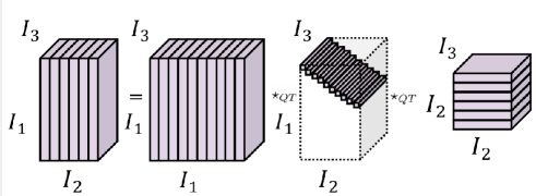
Figure 2: The illustration of the TQt-SVD of an $I_{1}\times I_{2}\times I_{3}$ quaternion tensor.

Algorithm 1 TQt-SVD based on $\star_{QT}$-product

0:  $\dot{\mathcal{T}}\in\mathbb{H}^{I_{1}\times I_{2}\times\times I_{3}}$, and invertible quaternion matrix $\dot{\mathbf{Q}}_{3}\in\mathbb{H}^{I_{3}\times I_{3}}$.

1:  Compute $\hat{\dot{\mathcal{T}}}=\mathit{L}(\dot{\mathcal{T}})=\dot{\mathcal{T}}\times_{3}\dot{\mathbf{Q}}_{3}$

2:  Compute each frontal slice of $\hat{\dot{\mathcal{U}}}$, $\hat{\dot{\mathcal{D}}}$, $\hat{\dot{\mathcal{V}}}$ from $\hat{\dot{\mathcal{T}}}$ byfor $i=1,\cdots,n_{3}$ do$[\hat{\dot{\mathcal{U}}}^{(i)},\hat{\dot{\mathcal{D}}}^{(i)},\hat{\dot{\mathcal{V}}}^{(i)}]=QSVD(\hat{\dot{\mathcal{T}}}^{(i)})$;end for

3:  Compute $\dot{\mathcal{U}}=\mathit{L}^{-1}(\hat{\dot{\mathcal{U}}}),\dot{\mathcal{D}}=\mathit{L}^{-1}(\hat{\dot{\mathcal{D}}}),\dot{\mathcal{V}}=\mathit{L}^{-1}(\hat{\dot{\mathcal{V}}}).$

3:  TQt-SVD components $\dot{\mathcal{U}},\dot{\mathcal{D}}$, and $\dot{\mathcal{V}}$ of $\dot{\mathcal{T}}$.

From Theorem 1, it can be concluded that the diagonal matrix is real such that the f-diagonal quaternion tensor in TQt-SVD is a real quaternion tensor in the transform domain. Moreover, it can be observed that the singular values of $\dot{\mathcal{T}}^{(i)}$ and $\dot{\mathcal{D}}^{(i)}$ are the same, whiche are the elements on the diagonal of $\dot{\mathcal{D}}^{(i)}$. Based on the above discussion, the quaternion tensor nuclear norm is defined for three-dimensional quaternion tensor as follows.

Definition 6 (quaternion tensor tubal rank and nuclear norm (QTNN))

For $\dot{\mathcal{T}}\in\mathbb{H}^{I_{1}\times I_{2}\times\times I_{3}}$, its corresponding TQt-SVD is $\dot{\mathcal{T}}=\dot{\mathcal{U}}\star_{QT}\dot{\mathcal{D}}\star_{QT}\dot{\mathcal{V}}^{H}$. The tubal rank of $\dot{\mathcal{T}}$ is defined as the maximum rank among all frontal slices of the f-diagonal quaternion tensor $\hat{\dot{\mathcal{D}}}$ i.e., $rank_{TQt}(\dot{\mathcal{T}})=\max_{i}\{rank(\dot{\mathcal{D}}^{(i)})\}$. The quaternion tensor nuclear norm is defined as the sum of singular values of $\dot{\mathcal{T}}$, i.e., $\parallel\dot{\mathcal{T}}\parallel_{*}=\sum_{i=1}^{I_{3}}\sum_{j=1}^{\min\{I_{1},I_{2}\}}\sigma_{j}(\dot{\mathcal{T}}^{(i)})=\sum_{i=1}^{I_{3}}\sum_{j=1}^{\min\{I_{1},I_{2}\}}\sigma_{j}(\dot{\mathcal{D}}^{(i)})=tr(\dot{\mathcal{T}})$.

As highlighted in [26], the largest singular values do not affect the rank of target matrix.Various works were inspired by it and subsequently improved the efficacy of image completion [8, 27]. Furthermore, the quaternion tensor truncated nuclear norm is proposed as follows.

Definition 7 (quaternion tensor truncated nuclear norm (QT-RNN))

For $\dot{\mathcal{T}}\in\mathbb{H}^{I_{1}\times I_{2}\times\times I_{3}}$, the QT-RNN is defined as $\|\dot{\mathcal{T}}\|_{r}=\sum_{i=1}^{I_{3}}\sum_{j=r+1}^{\min\{I_{1},I_{2}\}}\sigma_{j}(\dot{\mathcal{T}}^{(i)}).$

Motivated by the superior performance of logarithmic function acts on singular values compared to NN [28, 29, 11], the quaternion tensor Logarithmic norm (QTLN) is defined as follows.

Definition 8 (QTLN)

Given $\dot{\mathcal{T}}\in\mathbb{H}^{I_{1}\times I_{2}\times\times I_{3}}$, the logarithmic norm of the quaternion tensor with $0<p\leq 1$ and $\epsilon>0$ is:

$$\parallel\dot{\mathcal{T}}\parallel_{L}^{p}=\sum_{i=1}^{\min(M,N)}\log(\sigma_{i}^{p}(\dot{\mathcal{T}})+\epsilon),$$ (2)

where $\sigma_{i}$ can be obtained by the TQt-SVD of $\dot{\mathcal{T}}$.

The logarithmic function can flexibly control the penalization of singular values, which is consistent with the operation that larger singular values should be punished less (because the larger the singular value, the less it will affect the judgment of the rank) and correspondingly, smaller singular values should be punished more.

III-B Sparsity of The Underlying Quaternion Tensor

Many nature signals are sparse, like audios, images, and videos, and such property can be characterized in a certain transformed domain [20]. Motivated by these factors, in this section, the QTDCT is defined without destroying the structure of the quaternion tensor and the practical steps are listed.

Definition 9 (QTDCT)

As the non-commutative multiplication of quaternions, QTDCT has two forms, left-handed form $\text{QTDCT}_{L}(\mathcal{C}(\cdot)_{L})$ and right-handed form $\text{QTDCT}_{R}(\mathcal{C}(\cdot)_{R})$. They satisfy the following formulas, respectively. Let $\dot{\mathcal{T}}\in\mathbb{H}^{I_{1}\times I_{2}\times\times I_{3}}$ be a input signal, the transformed output quaternion tensor $\mathcal{C}(\dot{\mathcal{T}})\in\mathbb{H}^{I_{1}\times I_{2}\times\times I_{3}}$ is given by:

$$\mathcal{C}(\dot{\mathcal{T}})_{L}\triangleq\dot{u}\cdot(\dot{\mathcal{T}}\times_{1}\mathbf{C}_{1}\times_{2}\mathbf{C}_{2}\times_{3}\mathbf{C}_{3})$$ (3)

$$\mathcal{C}(\dot{\mathcal{T}})_{R}\triangleq(\dot{\mathcal{T}}\times_{1}\mathbf{C}_{1}\times_{2}\mathbf{C}_{2}\times_{3}\mathbf{C}_{3})\cdot\dot{u},$$ (4)

where $\dot{u}$ is a pure quaternion and meets $\dot{u}^{2}=-1$, and $\mathbf{C}_{i}\in\mathbb{R}^{I_{i}\times I_{i}},i=1,2,3.$ are DCT matrix as described in [30].

Corresponding to QTDCT, there are two forms of inverse transformation of QTDCT (denoted as $\mathcal{C}^{-1}(\cdot)_{L}$ and $\mathcal{C}^{-1}(\cdot)_{R}$). They satisfy the following formulas, respectively:

$$\mathcal{C}^{-1}(\dot{\mathcal{T}})_{L}\triangleq\dot{u}\cdot(\dot{\mathcal{T}}\times_{1}\mathbf{C}_{1}^{-1}\times_{2}\mathbf{C}_{2}^{-1}\times_{3}\mathbf{C}_{3}^{-1})$$ (5)

$$\mathcal{C}^{-1}(\dot{\mathcal{T}})_{R}\triangleq(\dot{\mathcal{T}}\times_{1}\mathbf{C}_{1}^{-1}\times_{2}\mathbf{C}_{2}^{-1}\times_{3}\mathbf{C}_{3})^{-1}\cdot\dot{u},$$ (6)

$\mathcal{C}(\dot{\mathcal{T}})$ and $\mathcal{C}^{-1}(\dot{\mathcal{T}})$ are the transformation pairs of each other.

In the developed algorithm, $\text{QTDCT}_{L}$ is utilized to carry out QTDCT. A better explanation of the efficiency of $\text{QTDCT}_{L}$ is that it is used to depict the sparsity of the target quaternion tensor. In Fig. 3, the modulus of each pixel of the color video stream is drawn. Typically, the modulus of the pixels of the color video stream tend zero after QTDCT transformation, which means that the video stream is sparse in the transform domain. This is the sparse regularization which is employed in the proposed algorithm. Taking advantage of the Cayley Dickson notation and motivating by the matrix form in Definition 1, all steps of $\text{QTDCT}_{L}$ are listed as follows:

1. Transforming the given quaternion tensor $\dot{\mathcal{T}}\in\mathbb{H}^{I_{1}\times I_{2}\times\times I_{3}}$ to the Cayley Dickson form $\dot{\mathcal{T}}=\mathcal{T}_{p}+\mathcal{T}_{q}j$, where $\mathcal{T}_{p}$ and $\mathcal{T}_{q}\in\mathbb{C}^{I_{1}\times I_{2}\times\times I_{3}}$.

2. Calculating the multidimensional DCT of complex tensors $\mathcal{T}_{p}$ and $\mathcal{T}_{q}$. The results are denoted as $\text{DCT}_{C}(\mathcal{T}_{p})$ and $\text{DCT}_{C}(\mathcal{T}_{q})$, respectively.

3. According to Cayley Dickson theorem, $\text{DCT}_{C}(\mathcal{T}_{p})$ and $\text{DCT}_{C}(\mathcal{T}_{q})$ can form a quaternion tensor: $\hat{\mathcal{C}}(\dot{\mathcal{T}})_{L}=\text{DCT}_{C}(\mathcal{T}_{p})+\text{DCT}_{C}(\mathcal{T}_{q})j$.

4. Multiplying $\mathcal{C}(\dot{\mathcal{T}})_{L}$ with the unit quaternion factor $\dot{u}$ to obtain the final result $\mathcal{C}(\dot{\mathcal{T}})_{L}=\dot{u}\cdot\hat{\mathcal{C}}(\dot{\mathcal{T}})_{L}$.

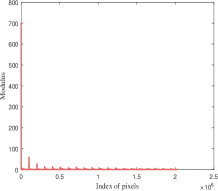
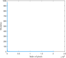
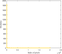
Figure 3: The illustration of the sparsity under QTDCT, taking three color videos (each video has 20 frames) as examples.

IV The corresponding recovery models and Algorithm

This section is divided into two parts. Subsection IV-A gives the formulation of the proposed recovery model, while subsection IV-B presents the two-step optimization with ADMM.

IV-A Problem Formulation

This section gives the formulation of low-rank quaternion tensor optimized model for color video recovery.

Similar to completion models based on low-rank constraints, thee low-rank quaternion tensor completion also utilizes low rankness as previously detailed to build the relationship between the observed and the missing elements in the target quaternion tensor. Mathematically, the recovery model can be formulated as follows.

$$\min\limits_{\dot{\mathcal{T}}}\text{rank}(\dot{\mathcal{T}})$$ (7)

$$\text{ s.t.}\quad P_{\Omega}(\dot{\mathcal{T}})=P_{\Omega}(\dot{\mathcal{O}}),$$

where $\dot{\mathcal{T}}$ is the underlying quaternion tensor, $\dot{\mathcal{O}}$ is the observed quaternion tensor, $\Omega$ is the index set for observed elements. $P_{\Omega}$ is a linear operation that indicates the elements in $\Omega$ are unchanged and zeros out others.

In the existing research, there has been extensive discussion of the nuclear norm (sum of the singular values) as the tightest convex substitute of rank. Moreover, the first few largest singular values do not affect the rank, hence, the QT-RNN which proposed in Definition 7 is adopted to replace the nuclear norm. Additionally, the sparsity as a vital property is considered in the recovery model by the designed regularization under QTDCT. Subsequently, the QT-RNN with sparsity (QT-RNNS) model can be written as follows.

$$\min\limits_{\dot{\mathcal{T}}}\parallel\dot{\mathcal{T}}\parallel_{r}+\lambda\parallel\dot{\mathcal{S}}\parallel_{1}$$ (8)

$$\text{s.t.}\quad P_{\Omega}(\dot{\mathcal{T}})=P_{\Omega}(\dot{\mathcal{O}}),\dot{\mathcal{S}}=\mathcal{C}(\dot{\mathcal{T}})_{L},$$

where $\parallel\dot{\mathcal{T}}\parallel_{r}=\sum_{i=1}^{I_{3}}\sum_{j=r+1}^{\min\{I_{1},I_{2}\}}\sigma_{j}(\dot{\mathcal{T}}^{(i)})=\sum_{i=1}^{I_{3}}\sum_{j=1}^{\min\{I_{1},I_{2}\}}\sigma_{j}(\dot{\mathcal{T}}^{(i)})-\sum_{i=1}^{I_{3}}\sum_{j=1}^{r}\sigma_{j}(\dot{\mathcal{T}}^{(i)})=\parallel\dot{\mathcal{T}}\parallel_{*}-\sum_{i=1}^{I_{3}}\sum_{j=1}^{r}\sigma_{j}(\dot{\mathcal{T}}^{(i)})$, $\dot{\mathcal{S}}$ is the transformed quaternion tensor, $\mathcal{C}(\cdot)$ is the QTDCT transform operator, and $\lambda$ is a positive number.

Basing on the Theorem 3 in [27], the equation in model (8) can be rewritten as

$$\min\limits_{\dot{\mathcal{T}}}\parallel\dot{\mathcal{T}}\parallel_{*}-\sum_{i=1}^{I_{3}}\mathop{\max}\limits_{\dot{\mathbf{A}}^{(i)}\dot{\mathbf{A}}^{(i)H}=\mathbf{I},\atop\dot{\mathbf{B}}^{(i)}\dot{\mathbf{B}}^{(i)H}=\mathbf{I}}|tr(\dot{\mathbf{A}}^{(i)}\dot{\mathcal{T}}^{(i)}\dot{\mathbf{B}}^{(i)H})|+\lambda\parallel\dot{\mathcal{S}}\parallel_{1}$$ (9)

$$\text{s.t.}\quad P_{\Omega}(\dot{\mathcal{T}})=P_{\Omega}(\dot{\mathcal{O}}),\dot{\mathcal{S}}=\mathcal{C}(\dot{\mathcal{T}})_{L},$$

where $\dot{\mathbf{A}}^{(i)}$ and $\dot{\mathbf{B}}^{(i)}$ are combined by the first r columns of $\dot{\mathcal{U}}^{(i)}$ and $\dot{\mathcal{V}}^{(i)}$ respectively, which are the left and right unitary matrices of $\dot{\mathcal{T}}^{(i)}$. Besides, based on the definition of $\star_{QT}$-product in Definition 4, (9) can be converted to

$$\min\limits_{\dot{\mathcal{T}}}\parallel\dot{\mathcal{T}}\parallel_{*}-\mathop{\max}\limits_{\dot{\mathcal{A}}\star_{QT}\dot{\mathcal{A}}^{H}=\dot{\mathcal{I}},\atop\dot{\mathcal{B}}\star_{QT}\dot{\mathcal{B}}^{H}=\dot{\mathcal{I}}}|tr(\dot{\mathcal{A}}\star_{QT}\hat{\dot{\mathcal{T}}}\star_{QT}\dot{\mathcal{B}}^{H})|+\lambda\parallel\dot{\mathcal{S}}\parallel_{1}$$ (10)

$$\text{s.t.}\quad P_{\Omega}(\dot{\mathcal{T}})=P_{\Omega}(\dot{\mathcal{O}}),\dot{\mathcal{S}}=\mathcal{C}(\dot{\mathcal{T}})_{L},$$

where $\dot{\mathcal{I}}$ is the identity quaternion tensor whose each frontal slice is the quaternion matrix. $\dot{\mathcal{A}}$ and $\dot{\mathcal{B}}$ is derived from the first $r$ columns of the second dimension of $\dot{\mathcal{U}}$ and $\dot{\mathcal{V}}$, respectively. Using Matlab notation, $\dot{\mathcal{A}}$ and $\dot{\mathcal{B}}$ can be denoted as follows

$$\dot{\mathcal{A}}\triangleq\dot{\mathcal{U}}(:,1:r,:)^{H},\quad\dot{\mathcal{B}}\triangleq\dot{\mathcal{V}}(:,1:r,:)^{H}.$$ (11)

Thus, after obtaining $\dot{\mathcal{A}}$ and $\dot{\mathcal{B}}$ in the first step, the main purpose is to solve (10) in the second step. The two-step based method is summarized in Algorithm 2.

Algorithm 2 Low-rank Quaternion Recovery with Sparse Regularization

0:  the observed incomplete quaternion tensor $\dot{\mathcal{O}}\in\mathbb{H}^{I_{1}\times I_{2}\times I_{3}}$; the index set of observed elements $\Omega$; the tolerance $\varepsilon_{0}$.

1:  Initialize the initial number of iteration $l=1$, $\dot{\mathcal{T}}_{1}=\dot{\mathcal{O}}$.

2:  Repeat

3:   Step 1. Calculating the QTt-SVD of the given $\dot{\mathbf{T}}_{l}$      $[\dot{\mathcal{U}}_{l},\mathcal{D}_{l},\dot{\mathcal{V}}_{l}]=\text{QTt-SVD }(\dot{\mathcal{T}}_{l})$, where $\dot{\mathcal{U}}_{l}\in\mathbb{H}^{I_{1}\times I_{1}\times I_{3}}$, $\dot{\mathcal{V}}_{l}\in\mathbb{H}^{I_{2}\times I_{2}\times I_{3}}$ are the unitary  quaternion tensor.

4:   Calculating $\dot{\mathcal{A}}_{l}$ and $\dot{\mathcal{B}}_{l}$ as follows $\dot{\mathcal{A}}_{l}\triangleq\dot{\mathcal{U}}_{l}(:,1:r,:)^{H},\dot{\mathcal{B}}_{l}\triangleq\dot{\mathcal{V}}_{l}(:,1:r,:)^{H}.$

5:   Step 2. Solving the optimization problem as follows   $\dot{\mathcal{T}}_{l+1}=\arg\min\limits_{\dot{\mathcal{T}}}\parallel\dot{\mathcal{T}}\parallel_{*}-|tr(\dot{\mathcal{A}}_{l}\star_{QT}\dot{\mathcal{T}}\star_{QT}\dot{\mathcal{B}}_{l}^{H})|$     $+\lambda\parallel\dot{\mathcal{S}}\parallel_{1}$,  $\text{s.t.}\quad P_{\Omega}(\dot{\mathcal{T}})=P_{\Omega}(\dot{\mathcal{O}})\qquad\mathcal{C}(\dot{\mathcal{T}})=\dot{\mathcal{S}}.$

6:  Until convergence $\|\dot{\mathcal{T}}_{l+1}-\dot{\mathcal{T}}_{l}\|_{F}\leq\varepsilon_{0}$, $\dot{\mathcal{T}}_{opt}=\dot{\mathcal{T}}_{l+1}$.

6:  the recovered quaternion tensor $\dot{\mathcal{T}}_{opt}$.

IV-B ADMM-based optimization

Next, the goal is to optimize problem (10). The ADMM framework is employed to solve this problem. Firstly, an auxiliary variable is introduced $\dot{\mathcal{H}}$ and reformulating (10) as

$$\min\limits_{\dot{\mathcal{T}}}\parallel\dot{\mathcal{T}}\parallel_{*}-\mathop{\max}\limits_{\dot{\mathcal{A}}\star_{QT}\dot{\mathcal{A}}^{H}=\dot{\mathcal{I}},\atop\dot{\mathcal{B}}\star_{QT}\dot{\mathcal{B}}^{H}=\dot{\mathcal{I}}}|tr(\dot{\mathcal{A}}\star_{QT}\hat{\dot{\mathcal{H}}}\star_{QT}\dot{\mathcal{B}}^{H})|+\lambda\parallel\dot{\mathcal{S}}\parallel_{1}$$ (12)

$$\text{s.t.}\quad P_{\Omega}(\dot{\mathcal{T}})=P_{\Omega}(\dot{\mathcal{O}}),\dot{\mathcal{H}}=\dot{\mathcal{T}},\dot{\mathcal{S}}=\mathcal{C}(\dot{\mathcal{T}})_{L}.$$

Inspiring by the ADMM framework utilized in the quaternion domain [31]. The corresponding augmented Lagrangian function of (12) can be written as

$$\begin{split}&\mathcal{L}(\dot{\mathcal{T}},\dot{\mathcal{H}},\dot{\mathcal{S}},\dot{\mathcal{Y}},\dot{\mathcal{Z}},\beta)=\\ &\parallel\dot{\mathcal{T}}\parallel_{*}-|tr(\dot{\mathcal{A}}_{l}\star_{QT}\dot{\mathcal{H}}\star_{QT}\dot{\mathcal{B}}_{l}^{H})|+\lambda\parallel\dot{\mathcal{S}}\parallel_{1}\\ &+\mathfrak{R}(\langle\dot{\mathcal{Y}},\dot{\mathcal{T}}-\dot{\mathcal{H}}\rangle)+\frac{\beta}{2}\parallel\dot{\mathcal{T}}-\dot{\mathcal{H}}\parallel_{F}^{2}\\ &+\mathfrak{R}(\langle\dot{\mathcal{Z}},\dot{\mathcal{S}}-\mathcal{C}(\dot{\mathcal{T}})_{L})+\frac{\beta}{2}\parallel\dot{\mathcal{S}}-\mathcal{C}(\dot{\mathcal{T}})_{L}\parallel_{F}^{2},\end{split}$$ (13)

where $\dot{\mathcal{Y}}$ and $\dot{\mathcal{Z}}$ are Lagrange multipliers, and $\beta$ is a positive penalty parameter. With utilization of ADMM algorithm, in the $k$-th iteration, (13) can be rewritten as

$$\left\{\begin{array}[]{lr}\dot{\mathcal{T}}^{k+1}=\arg\min\limits_{\dot{\mathcal{T}}}\mathcal{L}(\dot{\mathcal{T}},\dot{\mathcal{H}}^{k},\dot{\mathcal{S}}^{k},\dot{\mathcal{Y}}^{k},\dot{\mathcal{Z}}^{k},\beta^{k}),&\\ \dot{\mathcal{S}}^{k+1}=\arg\min\limits_{\dot{\mathcal{S}}}\mathcal{L}(\dot{\mathcal{T}}^{k+1},\dot{\mathcal{H}}^{k},\dot{\mathcal{S}},\dot{\mathcal{Y}}^{k},\dot{\mathcal{Z}}^{k},\beta^{k}),\\ \dot{\mathcal{H}}^{k+1}=\arg\min\limits_{\dot{\mathcal{H}}}\mathcal{L}(\dot{\mathcal{T}}^{k+1},\dot{\mathcal{H}},\dot{\mathcal{S}}^{k+1},\dot{\mathcal{Y}}^{k},\dot{\mathcal{Z}}^{k},\beta^{k}),\\ \dot{\mathcal{Y}}^{k+1}=\dot{\mathcal{Y}}^{k}+\beta^{k}(\dot{\mathcal{T}}^{k+1}-\dot{\mathcal{H}}^{k+1}),\\ \dot{\mathcal{Z}}^{k+1}=\dot{\mathcal{Z}}^{k}+\beta^{k}(\dot{\mathcal{S}}^{k+1}-\mathcal{C}(\dot{\mathcal{T}}^{k+1})_{L}).\end{array}\right.$$ (14)

1. The $\dot{\mathcal{T}}^{k+1}$ subproblem is

$$\begin{split}\dot{\mathcal{T}}^{k+1}&=\arg\min\limits_{\dot{\mathcal{T}}}\parallel\dot{\mathcal{T}}\parallel_{*}+\mathfrak{R}(\langle\dot{\mathcal{Y}}^{k},\dot{\mathcal{T}}-\dot{\mathcal{H}}^{k}\rangle)+\frac{\beta^{k}}{2}\parallel\dot{\mathcal{T}}-\dot{\mathcal{H}}^{k}\parallel_{F}^{2}\\ &\quad+\mathfrak{R}(\langle\dot{\mathcal{Z}}^{k},\dot{\mathcal{S}}^{k}-\mathcal{C}(\dot{\mathcal{T}}^{k})_{L})+\frac{\beta^{k}}{2}\parallel\dot{\mathcal{S}}^{k}-\mathcal{C}(\dot{\mathcal{T}})_{L}\parallel_{F}^{2}\\ &=\arg\min\limits_{\dot{\mathcal{T}}}\parallel\dot{\mathcal{T}}\parallel_{*}+\frac{\beta^{k}}{2}\parallel\dot{\mathcal{T}}-\dot{\mathcal{H}}^{k}+\dot{\mathcal{Y}}^{k}/\beta^{k}\parallel_{F}^{2}\\ &\quad+\frac{\beta^{k}}{2}\parallel\dot{\mathcal{S}}^{k}-\mathcal{C}(\dot{\mathcal{T}})_{L}+\dot{\mathcal{Z}}^{k}/\beta^{k}\parallel_{F}^{2}.\end{split}$$ (15)

Although, in the last term of (15), $\dot{\mathcal{T}}$ can not be separated directly since the transformation $\mathcal{C}$. The Parseval theorem is established in the quaternion domain, which demonstrates that after transforming the total energy of the signal is unchanged [32, 33]. This allows the last term to be computed in either the spatial domain or the quaternion domain. Thus the Frobenius norm in the last term of (15) can be rewritten as

$$\begin{split}\parallel\dot{\mathcal{S}}^{k}-\mathcal{C}(\dot{\mathcal{T}})_{L}+\dot{\mathcal{Z}}^{k}/\beta^{k}\parallel_{F}^{2}=\parallel\mathcal{C}^{-1}(\dot{\mathcal{S}}^{k}+\dot{\mathcal{Z}}^{k}/\beta^{k})_{L}-\dot{\mathcal{T}}\parallel_{F}^{2}.\end{split}$$

Consequently, (15) can be rewritten as

$$\begin{split}\dot{\mathcal{T}}^{k+1}&=\arg\min\limits_{\dot{\mathcal{T}}}\parallel\dot{\mathcal{T}}\parallel_{*}+\frac{\beta^{k}}{2}\parallel\dot{\mathcal{T}}-\dot{\mathcal{H}}^{k}+\dot{\mathcal{Y}}^{k}/\beta^{k}\parallel_{F}^{2}\\ &\quad+\frac{\beta^{k}}{2}\parallel\mathcal{C}^{-1}(\dot{\mathcal{S}}^{k}+\dot{\mathcal{Z}}^{k}/\beta^{k})_{L}-\dot{\mathcal{T}}\parallel_{F}^{2}\\ &=\arg\min\limits_{\dot{\mathcal{T}}}\parallel\dot{\mathcal{T}}\parallel_{*}\\ &\quad+\beta^{k}\parallel\dot{\mathcal{T}}-\frac{1}{2}[\dot{\mathcal{H}}^{k}+\dot{\mathcal{Y}}^{k}/\beta^{p}+\mathcal{C}^{-1}(\dot{\mathcal{S}}^{k}+\dot{\mathcal{Z}}^{k}/\beta^{k})]\parallel_{F}^{2}.\end{split}$$ (16)

To solve (16), the Quaternion Tensor Singular Value Thresholding (QTSVT) is defined as follows

Definition 10 (QTSVT)

Let $\dot{\mathcal{X}}=\dot{\mathcal{U}}\star_{QT}\dot{\mathcal{D}}\star_{QT}\dot{\mathcal{V}}^{H}$ be the QTt-SVD of $\dot{\mathcal{X}}$. For any $\tau>0$, the QTSVT operator is defined as

$$\mathfrak{D}_{\tau}(\dot{\mathcal{X}})=\dot{\mathcal{U}}\star_{QT}\dot{\mathcal{D}}_{\tau}\star_{QT}\dot{\mathcal{V}}^{H},$$ (17)

where $\dot{\mathcal{D}}_{\tau}=L^{-1}((L(\dot{\mathcal{D}})-\tau))_{+}$, and $(*)_{+}$ denotes the positive part of $*$.

Theorem 3

Let $L$ be the linear transform which is utilized in TQt-SVD, for any $\tau>0$ and $\dot{\mathcal{X}}\in\mathbb{H}^{I_{1}\times I_{2}\times I_{3}}$, the TQSVT in (17) obeys

$$\mathfrak{D}_{\tau}(\dot{\mathcal{X}})=\arg\min\limits_{\dot{\mathcal{T}}}\tau\parallel\dot{\mathcal{T}}\parallel_{*}+\frac{1}{2}\parallel\dot{\mathcal{T}}-\dot{\mathcal{X}}\parallel_{F}^{2}.$$ (18)

Utilizing Theorem 3, (16) can be solved by

$$\dot{\mathcal{T}}^{k+1}=\mathfrak{D}_{\frac{1}{2\beta^{k}}}(\frac{1}{2}[\dot{\mathcal{H}}^{k}+\dot{\mathcal{Y}}^{k}/\beta^{k}+\mathcal{C}^{-1}(\dot{\mathcal{S}}^{k}+\dot{\mathcal{Z}}^{k}/\beta^{k})]).$$ (19)

It can be observed from (16) that the process of obtaining the update of $\dot{\mathcal{T}}^{k+1}$ is to find the optimized solution from the sum of QTNN and Frobenius norm. In this process, the QTNN also implies that all the singular values are treated equally, to optimize this problem and get a more precise approximation of the rank, the QTNN is further replaced by QTLN in (16). In this way, (16) can be reformulated as

$$\begin{split}\dot{\mathcal{T}}^{k+1}&=\arg\min\limits_{\dot{\mathcal{T}}}\parallel\dot{\mathcal{T}}\parallel_{L}+\frac{\beta^{k}}{2}\parallel\dot{\mathcal{T}}-\dot{\mathcal{H}}^{k}+\dot{\mathcal{Y}}^{k}/\beta^{k}\parallel_{F}^{2}\\ &\quad+\frac{\beta^{k}}{2}\parallel\mathcal{C}^{-1}(\dot{\mathcal{S}}^{k}+\dot{\mathcal{Z}}^{k}/\beta^{k})_{L}-\dot{\mathcal{T}}\parallel_{F}^{2}\\ &=\arg\min\limits_{\dot{\mathcal{T}}}\parallel\dot{\mathcal{T}}\parallel_{L}\\ &\quad+\beta^{k}\parallel\dot{\mathcal{T}}-\frac{1}{2}[\dot{\mathcal{H}}^{k}+\dot{\mathcal{Y}}^{k}/\beta^{p}+\mathcal{C}^{-1}(\dot{\mathcal{S}}^{k}+\dot{\mathcal{Z}}^{k}/\beta^{k})]\parallel_{F}^{2}.\end{split}$$ (20)

For solving (20), similar to the real cases [29], the theorem of Quaternion Tensor Logarithmic Singular Value Thresholding (QTLSVT) is given as follows

Theorem 4 (QTLSVT)

For any quaternion tensor $\dot{\mathcal{X}}\in\mathbb{H}^{I_{1}\times I_{2}\times I_{3}}$ and $\lambda>0$, the QTt-SVDt is $\dot{\mathcal{X}}=\dot{\mathcal{U}}\star_{QT}\dot{\mathcal{D}}\star_{QT}\dot{\mathcal{V}}^{H}$. Then the closed solution of the following problem

$$\mathop{\arg\min}\limits_{\dot{\mathcal{T}}}\lambda\parallel\dot{\mathcal{T}}\parallel_{L}^{1}+\frac{1}{2}\parallel\dot{\mathcal{T}}-\dot{\mathcal{X}}\parallel_{F}^{2}$$ (21)

is provided by $\dot{\mathcal{U}}\star_{QT}\dot{\mathcal{L}}_{\lambda,\epsilon}\star_{QT}\dot{\mathcal{V}}^{H}$, where $\dot{\mathcal{L}}_{\lambda,\epsilon}(\dot{\mathcal{D}}_{\dot{\mathcal{X}}})=L^{-1}(\mathcal{L}_{\lambda,\epsilon}(L(\dot{\mathcal{D}})))$. The soft thresholding operator $\mathcal{L}_{\lambda,\epsilon}(\cdot)$ is defined as:

$$\mathcal{L}_{\lambda,\epsilon}(x)=\begin{cases}0,\qquad\qquad\qquad\qquad\qquad\Delta\leq 0\\ \mathop{\arg\min}\limits_{a\in\{0,\frac{1}{2}(x-\epsilon+\sqrt{\Delta})\}}\textit{h}(a),\qquad\Delta>0,\end{cases}$$ (22)

where $\Delta=(x-\epsilon)^{2}-4(\lambda-x\epsilon)$, and function $\mathit{h}(a):=\frac{1}{2}(a-x)^{2}+\lambda\log(a+\epsilon)$ is $\mathbb{R}^{+}\longrightarrow\mathbb{R}^{+}$.

Utilizing Theorem 4, (20) can be solved by

$$\dot{\mathcal{T}}^{k+1}=\dot{\mathcal{U}}\star_{QT}\dot{\mathcal{L}}_{\lambda,\epsilon}(\dot{\mathcal{D}}_{\dot{\mathcal{A}}})\star_{QT}\dot{\mathcal{V}}^{H},$$ (23)

where $\dot{\mathcal{A}}^{k}=\frac{1}{2}[\dot{\mathcal{H}}^{k}+\dot{\mathcal{Y}}^{k}/\beta^{k}+\mathcal{C}^{-1}(\dot{\mathcal{S}}^{k}+\dot{\mathcal{Z}}^{k}/\beta^{k})]$.

2. The $\dot{\mathcal{S}}^{k+1}$ subproblem is

$$\begin{split}\dot{\mathcal{S}}^{k+1}&=\arg\min\limits_{\dot{\mathcal{S}}}\lambda\parallel\dot{\mathcal{S}}\parallel_{1}+\mathfrak{R}(\langle\dot{\mathcal{Z}}^{k},\dot{\mathcal{S}}-\mathcal{C}(\dot{\mathcal{T}}^{k+1})_{L})\\ &\quad+\frac{\beta}{2}\parallel\dot{\mathcal{S}}-\mathcal{C}(\dot{\mathcal{T}}^{k+1})_{L}\parallel_{F}^{2}\\ &=\arg\min\limits_{\dot{\mathcal{S}}}\lambda\parallel\dot{\mathcal{S}}\parallel_{1}+\frac{\beta^{k}}{2}\parallel\dot{\mathcal{S}}-\mathcal{C}(\dot{\mathcal{T}}^{k+1})+\dot{\mathcal{Z}}^{k}/\beta^{k}\parallel_{F}^{2}\\ &\end{split}$$ (24)

Because in the quaternion domain the closed solution of $\min\limits_{\dot{\mathbf{X}}}\lambda\parallel\dot{\mathbf{X}}\parallel_{1}+\parallel\dot{\mathbf{Y}}-\dot{\mathbf{X}}\parallel_{F}^{2}$ is given by $\dot{\mathbf{X}}_{opt}=\mathcal{S}_{2\lambda}(\dot{\mathbf{Y}})$ [34], analogously, problem (24) has a closed-form solution given by

$$\dot{\mathcal{S}}^{k+1}=\mathcal{S}_{\frac{4\lambda}{\beta^{k}}}(\mathcal{C}(\dot{\mathcal{T}}^{k+1})-\dot{\mathcal{Z}}^{k}/\beta^{k}).$$ (25)

3. The $\dot{\mathcal{H}}^{k+1}$ subproblem is

$$\begin{split}\dot{\mathcal{H}}^{k+1}&=\arg\min\limits_{\dot{\mathcal{H}}}-|tr(\dot{\mathcal{A}}_{l}\star_{QT}\dot{\mathcal{H}}\star_{QT}\dot{\mathcal{B}}_{l}^{H})|\\ &\quad+\mathfrak{R}(\langle\dot{\mathcal{Y}}^{k},\dot{\mathcal{T}}^{k+1}-\dot{\mathcal{H}}\rangle)\\ &\quad+\frac{\beta^{k}}{2}\parallel\dot{\mathcal{T}}^{k+1}-\dot{\mathcal{H}}\parallel_{F}^{2}.\end{split}$$ (26)

Because (26) is quadratic with respect to $\dot{\mathcal{H}}$, letting the derivation of (26) be zero, then the closed solution of $\dot{\mathcal{H}}$ can be written as

$$\dot{\mathcal{H}}^{k+1}=\dot{\mathcal{X}}^{k+1}+(\dot{\mathcal{Y}}^{k}+\dot{\mathcal{A}}^{H}\star_{QT}\dot{\mathcal{B}})/\beta^{k}.$$ (27)

Besides, let the observed elements remain unchanged in each iteration as follows

$$\dot{\mathcal{H}}^{k+1}=P_{\Omega^{C}}(\dot{\mathcal{H}}^{k+1})+P_{\Omega}(\dot{\mathcal{O}}).$$ (28)

4. The update of Lagrange multiplier $\dot{\mathcal{Y}}^{k+1}$

$$\dot{\mathcal{Y}}^{k+1}=\dot{\mathcal{Y}}^{k}+\beta^{k}(\dot{\mathcal{T}}^{k+1}-\dot{\mathcal{H}}^{k+1}),\\$$ (29)

5. The update of Lagrange multiplier $\dot{\mathcal{Z}}^{k+1}$

$$\dot{\mathcal{Z}}^{k+1}=\dot{\mathcal{Z}}^{k}+\beta^{k}(\dot{\mathcal{S}}^{k+1}-\mathcal{C}(\dot{\mathcal{T}}^{k+1})_{L}).$$ (30)

6. The update of penalty parameter $\beta^{k}$ is

$$\beta^{k+1}=\min\{\rho\beta^{k},\beta_{\max}\},$$ (31)

where $\rho\geq 1$ is a constant parameter to increase the penalty, and $\beta_{\max}$ is the upper bounded of $\beta$.

The QTSVT-based method is denoted as QT-RNNS1, and the logarithmic QTLSVT-based method is denoted as QT-RNNS2. The whole process in Step 2 is summarized in Algorithm 3.

Algorithm 3 The process of QT-RNNS1 and QT-RNNS2 in Step 2.

0:  $\dot{\mathcal{O}}$, $\Omega$, $\dot{\mathcal{A}}_{l}$, $\dot{\mathcal{B}}_{l}$, tolerance $\varepsilon$, and parameters $\lambda$, $\rho$, $\beta_{\max}$.

1:  Initial $\dot{\mathcal{X}}^{1}=\dot{\mathcal{O}}$, $\dot{\mathcal{H}}^{1}=\dot{\mathcal{D}}^{1}=\dot{\mathcal{X}}^{1}$, and $\beta^{1}$. Let $\dot{\mathcal{Y}}^{1}$ and $\dot{\mathcal{Z}}^{1}$ be random quaternion matrix with the same size of $\dot{\mathcal{X}}^{1}$.

2:  Repeat

3:  Update $\dot{\mathcal{X}}^{k+1}$$\dot{\mathcal{T}}^{k+1}=\mathfrak{D}_{\frac{1}{2\beta^{k}}}(\frac{1}{2}[\dot{\mathcal{H}}^{k}+\dot{\mathcal{Y}}^{k}/\beta^{k}+\mathcal{C}^{-1}(\dot{\mathcal{S}}^{k}+\dot{\mathcal{Z}}^{k}/\beta^{k})]).$ Or$\dot{\mathcal{T}}^{k+1}=\dot{\mathcal{U}}\star_{QT}\dot{\mathcal{L}}_{\lambda,\epsilon}(\dot{\mathcal{D}}_{\dot{\mathcal{A}}})\star_{QT}\dot{\mathcal{V}}^{H}$,where $\dot{\mathcal{A}}^{k}=\frac{1}{2}[\dot{\mathcal{H}}^{k}+\dot{\mathcal{Y}}^{k}/\beta^{k}+\mathcal{C}^{-1}(\dot{\mathcal{S}}^{k}+\dot{\mathcal{Z}}^{k}/\beta^{k})]$.

4:  Update $\dot{\mathcal{S}}^{k+1}=\mathcal{S}_{\frac{4\lambda}{\beta^{k}}}(\mathcal{C}(\dot{\mathcal{T}}^{k+1})-\dot{\mathcal{Z}}^{k}/\beta^{k}).$

5:  Update $\dot{\mathcal{H}}^{k+1}=\dot{\mathcal{X}}^{k+1}+(\dot{\mathcal{Y}}^{k}+\dot{\mathcal{A}}^{H}\star_{QT}\dot{\mathcal{B}})/\beta^{k},$   $\dot{\mathcal{H}}^{k+1}=P_{\Omega^{C}}(\dot{\mathcal{H}}^{k+1})+P_{\Omega}(\dot{\mathcal{O}}).$

6:  Update $\dot{\mathcal{Y}}^{k+1}=\dot{\mathcal{Y}}^{k}+\beta^{k}(\dot{\mathcal{T}}^{k+1}-\dot{\mathcal{H}}^{k+1}).$

7:  Update $\dot{\mathcal{Z}}^{k+1}=\dot{\mathcal{Z}}^{k}+\beta^{k}(\dot{\mathcal{S}}^{k+1}-\mathcal{C}(\dot{\mathcal{T}}^{k+1})_{L}).$

8:  Update $\beta^{k+1}=\min\{\rho\beta^{k},\beta_{\max}\}$.

9:  Until convergence $\|\dot{\mathcal{T}}^{k+1}-\dot{\mathcal{T}}^{k}\|_{F}\leq\varepsilon$ or $p$ reaches the given maximum iteration number.

9:  $\dot{\mathcal{T}}^{k+1}$

V Experimental Results

In this section, the proposed QT-RNNS1 and QT-RNNS2 methods are compared with seven related methods. Subsection V-A lists the experimental settings. Subsection V-B presents the color video recovery results. Subsection V-C provides a discussion of the experimental results.

V-A Experimental Settings

V-A1 Compared Methods

TNN [6], TNN-log [11], TNN-TV [35], TMac-inc and TMac-dec [36], TMac-TT[37], R-TNN[8], LRQTC [17]. The differences and relationships among all methods are listed in Table I.

TABLE I: The differences and relationships of the related methods.

Method	Representation of video	Description of low-rankness	Other prior information
TNN	tensor-based	tensor nuclear norm based on tensor SVD	-
TNN-log	tensor-based	sum of weighted logarithmic norm of mode-n unfolding matrices	-
TNN-TV	tensor-based	sum of nuclear norm based on Tucker decomposition	total variation regularization for local piecewise smooth structure
T-TNN	tensor-based	truncated tensor nuclear norm based on tensor SVD	-
TMac	tensor-based	low-rank matrix factorization based on Tucker decomposition	-
TMac-TT	tensor-based	low-rank matrix factorization based on Tensor Train decomposition	-
LRQTC	quaternion tensor-based	sum of weighted nuclear norm based on Tucker decomposition	-
QT-RNNS1	quaternion tensor-based	truncated nuclear norm based on TQt-SVD	sparse regularization based on QTDCT
QT-RNNS2	quaternion tensor-based	truncated nuclear norm with logarithmic norm based on TQt-SVD	sparse regularization based on QTDCT

V-A2 Test Data and Experimental Facility

Eight color videos were selected, including bus, akiyo, stefan, tempete, waterfall, suzie, container, and grandma . In the following experiments, only the first 20 frames are adopted, such that the first six videos are of size $288\times 352\times 3\times 20$ and the last three videos are of size $144\times 176\times 3\times 20$. They are reconstructed as pure quaternion tensors with sizes $288\times 352\times 20$ and $144\times 176\times 20$, respectively. The Sample Rates (SRs) are set to 50%, 30%, 20%, 10%, respectively. All the experiments were implemented in MATLAB R2019a, on a PC with a 3.00GHz CPU and 8GB RAM.

V-A3 Evaluation Indicators and Parameters Setting

Two indicators are employed to evaluate the performance of the proposed methods, including peak signal to noise rate (PSNR) and average structural similarity index (ASSIM). The parameters of QT-RNNS1 were set as $\beta^{1}=1e-1,\lambda=0.05,\rho=1.1$, and the parameters of QT-RNNS2 were set as $\beta^{1}=1e-1,\lambda=0.05,\rho=1.01$. Besides, based on the author’s codes, the parameters of other compared methods are adjusted to the best.

V-B Color Video Recovery Results

The PSNR and ASSIM are listed in Table II and Table III, and are obtained by all compared methods. The best numerical results are bolded. It can be observed that the proposed QT-RNNS2 can achieve the best results in most cases, except when SR$=0.5$ and SR$=0.3$, the QT-RNNS1 obtained the best PSNR values when recovering bus. Although QT-RNNS1 method is inferior to some tensor-based methods in some cases, the results are acceptable when compared to the quaternion-based methods .

Figure 4: The visual results of recovering bus with SR$=0.3$ at the 18th frame.

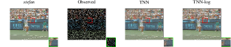
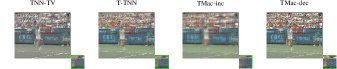
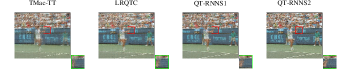
Figure 5: The visual results of recovering stefan with SR$=0.3$ at the 18th frame.

TABLE II: The $\frac{\text{PSNR}}{\text{ASSIM}}$comparison of different recovery methods for 8 color videos

Video	$\text{SR}=0.5$
	TNN	TNN-log	TNN-TV	T-TNN	TMac-inc	TMac-dec	TMac-TT	LRQTC	QT-RNNS1	QT-RNNS2
bus	27.4688 0.8472	27.8489 0.8520	26.7656 0.8848	27.5426 0.8481	22.5015 0.7017	26.0222 0.8118	23.5855 0.7589	27.0989 0.8767	28.1625 0.8916	29.3049 0.8792
akiyo	42.0237 0.9958	42.2329 0.9959	31.7104 0.9647	41.8984 0.9953	29.4959 0.9293	37.3297 0.9777	32.2096 0.9477	37.2693 0.9846	40.1668 0.9905	47.2225 0.9983
stefan	25.1503 0.9004	25.4682 0.9052	25.4945 0.9068	25.1899 0.9009	21.5793 0.8030	25.6508 0.9103	22.4252 0.8356	26.4100 0.9294	27.5370 0.9454	28.9896 0.9522
tempete	29.9098 0.9349	30.2200 0.9373	25.6139 0.8883	29.9513 0.9349	23.2665 0.7831	26.8717 0.8783	24.5690 0.8352	27.8278 0.9162	28.9693 0.9311	32.3476 0.9583
waterfall	36.2144 0.9837	36.4523 0.9844	29.4415 0.9358	36.2379 0.9837	28.0918 0.9077	31.7318 0.9543	29.4339 0.9318	32.6245 0.9678	35.1978 0.9802	39.8446 0.9921
suzie	37.0243 0.9844	37.2051 0.9849	32.1941 0.9515	36.9587 0.9840	31.9933 0.9531	20.8712 0.8327	34.1747 0.9683	34.6803 0.9756	35.4444 0.9773	40.1347 0.9908
container	39.2179 0.9924	39.4946 0.9927	26.5751 0.9202	38.8865 0.9918	27.9132 0.9249	18.4649 0.7712	31.6999 0.9635	30.9900 0.9668	32.4229 0.9722	47.3978 0.9974
grandma	46.2940 0.9986	46.4175 0.9986	30.0921 0.9540	46.1753 0.9986	31.3900 0.9613	24.5059 0.9213	36.2686 0.9862	36.1837 0.9877	36.6203 0.9889	47.9809 0.9990
Video	$\text{SR}=0.3$
	TNN	TNN-log	TNN-TV	T-TNN	TMac-inc	TMac-dec	TMac-TT	LRQTC	QT-RNNS1	QT-RNNS2
bus	23.7394 0.6998	24.2432 0.7123	23.2642 0.7453	23.8325 0.7016	22.9045 0.6080	21.7801 0.6850	23.4549 0.6487	24.5961 0.7331	25.7786 0.7823	29.3049 0.7713
akiyo	38.1462 0.9900	38.5320 0.9907	22.7441 0.8489	37.8275 0.9889	28.3054 0.9091	32.7141 0.9503	30.0190 0.9192	32.2587 0.9562	34.2534 0.9705	42.9540 0.9960
stefan	21.7232 0.7888	21.9902 0.7966	21.5849 0.7189	21.7321 0.7888	20.2946 0.7350	22.4055 0.8318	20.6749 0.7541	22.3532 0.8264	23.4745 0.8662	24.6364 0.8807
tempete	26.1205 0.8581	26.5584 0.8657	21.4621 0.7217	26.1117 0.8552	21.9732 0.7152	24.3118 0.7991	22.7670 0.7568	24.4188 0.8156	25.2774 0.8536	28.6686 0.9113
waterfall	32.3438 0.9620	32.7389 0.9647	22.1695 0.7371	32.2264 0.9607	26.8074 0.8792	26.8360 0.9064	27.6290 0.8973	29.0284 0.9288	30.8075 0.9483	35.9844 0.9816
suzie	33.3655 0.9668	33.7148 0.9686	26.9049 0.7988	32.9049 0.9631	30.4892 0.9366	15.8579 0.5306	31.9480 0.9492	30.8670 0.9498	31.3812 0.9496	36.6677 0.9809
container	35.2095 0.9823	35.7235 0.9837	23.0744 0.7725	34.4224 0.9800	26.5851 0.9001	12.4708 0.5230	29.0497 0.9360	26.5512 0.9151	27.1275 0.9217	42.3936 0.9939
grandma	43.0166 0.9971	43.3858 0.9973	22.8230 0.7525	42.6545 0.9968	30.1309 0.9488	19.4189 0.7586	33.5095 0.9742	31.4801 0.9669	31.5416 0.9683	45.1272 0.9980

TABLE III: The $\frac{\text{PSNR}}{\text{ASSIM}}$ comparison of different recovery methods for 8 color videos

Video	$\text{SR}=0.2$
	TNN	TNN-log	TNN-TV	T-TNN	TMac-inc	TMac-dec	TMac-TT	LRQTC	QT-RNNS1	QT-RNNS2
bus	21.8280 0.5931	22.3784 0.6113	21.5413 0.6319	21.9307 0.5953	20.4624 0.5495	18.4727 0.4981	20.9389 0.5807	21.6094 0.6346	22.7354 0.6967	24.0853 0.6986
akiyo	35.9674 0.9839	36.5191 0.9854	19.1079 0.6944	35.5094 0.9815	27.7474 0.8968	22.2224 0.7897	29.0119 0.9023	29.5693 0.9285	31.2501 0.9481	40.4373 0.9983
stefan	21.7232 0.7888	21.9902 0.7966	19.7294 0.5349	21.7321 0.7888	19.6133 0.6902	17.4463 0.6549	19.8573 0.7034	20.4872 0.7448	21.4389 0.7934	22.5682 0.8192
tempete	26.1205 0.8581	26.5584 0.8657	19.4599 0.5773	26.1117 0.8552	21.3331 0.6756	20.8422 0.6654	21.9784 0.7121	22.7217 0.7473	23.3364 0.7855	26.6932 0.8700
waterfall	32.3438 0.9620	32.7389 0.9647	19.1428 0.5020	17.7733 0.3313	32.2264 0.9607	22.8920 0.8426	26.8652 0.8781	27.0465 0.8924	28.6831 0.9184	33.6559 0.9697
suzie	31.4173 0.9507	31.9273 0.9547	24.4801 0.6262	30.6578 0.9415	29.6985 0.9253	12.6942 0.2244	30.7311 0.9345	28.6060 0.9145	28.9900 0.9222	34.6850 0.9706
container	32.7163 0.9710	33.4670 0.9744	21.3214 0.6191	31.5467 0.9639	25.7684 0.8817	9.9466 0.1523	27.5190 0.9130	24.1345 0.8566	24.5348 0.8703	38.6235 0.9885
grandma	19.0741 0.2940	19.0728 0.2956	19.7285 0.4841	19.0706 0.2930	29.4595 0.9400	16.5534 0.5292	32.0661 0.9646	28.6993 0.9414	28.8418 0.9462	43.2002 0.9970
Video	$\text{SR}=0.1$
	TNN	TNN-log	TNN-TV	T-TNN	TMac-inc	TMac-dec	TMac-TT	LRQTC	QT-RNNS1	QT-RNNS2
bus	19.6664 0.4522	19.9377 0.4590	19.5717 0.4828	19.4149 0.4350	19.5916 0.4686	14.0292 0.1959	19.7682 0.4854	19.3573 0.4897	19.4710 0.5314	21.9361 0.5863
akiyo	32.9523 0.9666	32.9349 0.9647	17.7276 0.5682	31.8867 0.9556	27.0762 0.8812	13.8732 0.4587	27.9046 0.8801	25.9348 0.8651	24.9418 0.8469	36.5933 0.9845
stefan	18.5912 0.6022	18.5178 0.5964	18.5187 0.5606	18.1608 0.5780	18.7304 0.6288	12.6956 0.2878	18.7689 0.6317	18.4741 0.6181	17.8973 0.6242	18.5270 0.6359
tempete	21.9430 0.6927	22.1501 0.7001	17.6936 0.4100	21.2944 0.6485	20.6303 0.6237	14.7226 0.3087	21.1393 0.6540	20.4420 0.6324	19.9407 0.6456	24.2331 0.7951
waterfall	27.5731 0.8948	27.6326 0.8963	17.9488 0.3211	26.5949 0.8757	25.4843 0.8409	16.8750 0.5648	26.0418 0.8546	24.8760 0.8355	25.7330 0.8565	30.4565 0.9414
suzie	28.7691 0.9193	29.1793 0.9234	22.4736 0.4667	26.5000 0.8780	28.3883 0.9057	9.9371 0.0592	28.8264 0.9094	25.0000 0.8500	23.2253 0.8156	31.9447 0.9496
container	28.2328 0.9331	28.1848 0.9300	19.4086 0.4668	25.0618 0.8808	23.4926 0.8337	7.1822 0.0333	24.8569 0.8624	21.4210 0.7439	18.7180 0.6174	31.9465 0.9647
grandma	15.0825 0. 5019	15.0834 0.5024	18.3090 0.2774	29.9678 0.9578	28.2759 0.9256	13.7822 0.2109	30.1074 0.9476	24.9565 0.8889	24.6477 0.8876	38.5849 0.9915

Figure 6: The visual results of recovering bus with SR=0.1 at the first frame.

Figure 7: The visual results of recovering akiyo with SR=0.1 at the first frame.

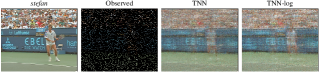
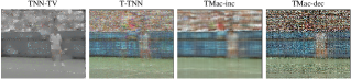
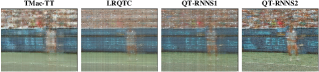
Figure 8: The visual results of recovering stefan with SR=0.1 at the first frame.

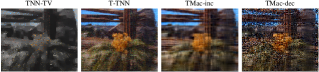
Figure 9: The visual results of recovering tempete with SR=0.1 at the first frame.

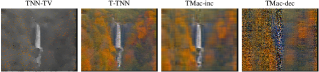
Figure 10: The visual results of recovering waterfall with SR=0.1 at the first frame.

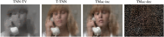
Figure 11: The visual results of recovering suzie with SR=0.1 at the first frame.

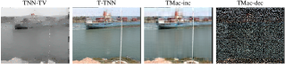
Figure 12: The visual results of recovering container with SR=0.1 at the first frame.

Figure 13: The visual results of recovering grandma with SR=0.1 at the first frame.

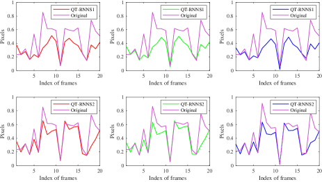
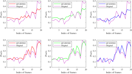
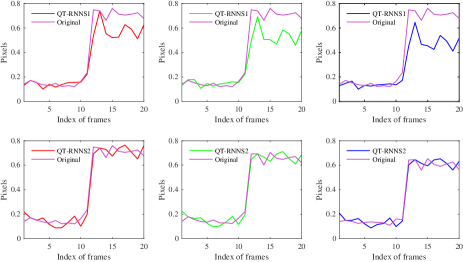
Figure 14: The pixels recovered results of color video bus by operating the proposed algorithms with SR$=0.1$. The first two rows are the pixels at the spatial location (206,100), the middle two rows are the pixels at the spatial location (220,300), and the bottom two rows are the pixels at the spatial location (11,16). The first, second, and third columns are the results for the red, green, and blue channels, respectively.

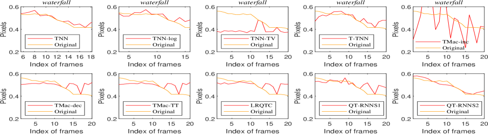
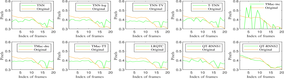
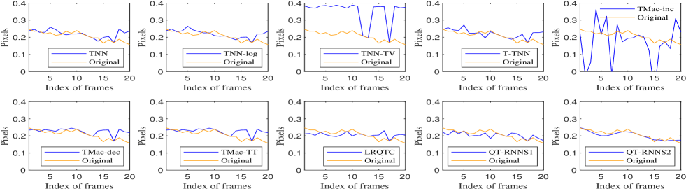
Figure 15: Comparison of the pixels recovered results of different algorithms with SR$=0.1$ at spatial location (153,104) of video waterfall. The first two rows are the results of the red channel, the middle two rows are the results of the green channel, and the bottom two rows are the blue channel.

The visual comparison is shown in Fig.4-Fig.5 in case of SR=$0.3$ (taking bus and stefan as examples). The picture in the green box in the lower right corner is the double magnification of the red box in the picture. As observed in Fig.4, the letters in the picture recovered by QT-RNNS2 are the most distinct. In Fig.5, it is possible to observe the tennis racket Stefan holding by carrying out QT-RNNS1 and QT-RNNS2.

In the case of SR=$0.1$, the visual comparison is shown in Fig.6-Fig.12. As can be seen, the results obtained by QT-RNNS2 have generally better visual effects than the recovered results obtained by other compared methods. The proposed method not only retains the global structure of the color video but also recovers its details. For example, it can be clearly observed from Fig. 8, stefan’s shoes can be seen in the recovered result of QT-RNNS2, while the recovery results of other methods are less visible.

In Fig. 14, the reconstructed pixel values of the color video bus at three spatial locations (206, 100), (220, 300), (11, 16) are shown. The pink curves represent the original pixels, whereas the red, green, and blue curves represent the recovered pixels.

Further, in Fig. 15, the reconstructed pixel values of the color video waterfall at one spatial location (153, 104) are shown. The yellow curves represent the original pixels, whereas the red, green, and blue curves are the recovered pixels. It can be observed that QT-RNNS2 can produce results that are the closest to the original curve. When the curves of QT-RNNS1 and QT-RNNS2 are compared, it is clear that the logarithmic function captures the rank function more well than other techniques.

V-C Discussions

The following is a summary of the discussion of the above experiment results:

• The developed QT-RNNS1 and QT-RNNS2 methods can achieve such excellent performance because they take into account both the global low rankness of color videos and the sparseness. Moreover, the quaternion tensor-based framework can prevent dimensionality reduction loss.

• In comparison to tensor-based methods: the proposed QT-RNNS1 and QT-RNNS2 are based on TQt-SVD which is comparable to tensor SVD in that the structure of color videos is preserved in the whole process. Besides, the simulation results demonstrate that the benefit of utilizing a truncated strategy and a logarithmic function to pursue a more accurate rank approximation is effectively implemented in newly created quaternion-based methods.

• In comparison to quaternion tensor-based methods: QT-RNNS1 and QT-RNNS2 are based on TQt-rank, and further approximation of the rank function improves the accuracy of the recovery results.

VI Conclusion

In this paper, a new quaternion tensor recover model was proposed for color video completion. The proposed method is based on TQt-rank, and then utilizes truncation and logarithmic function to obtain a more accurate low-rank restriction. A novel QTDCT was also developed to address the sparseness of color videos in the model. Furthermore, this regularization was induced by ${l_{1}}$ norm in the proposed model. A two-step optimization with ADMM framework was adopted to optimize the model. Experimental results for color videos recovery demonstrate the superiority of the proposed model. However, there remains significant room for improvement in color video recovery using quaternion tensors, such as introducing other decomposition methods in tensors (ring decomposition, fully-connect tensor network decomposition, etc.) into quaternion tensors, such as more in-depth exploration of the local properties of color video (smoothness, continuity, etc.).

References

• [1] J. Liu, P. Musialski, P. Wonka, and J. Ye, “Tensor completion for estimating missing values in visual data,” IEEE Trans. Pattern Anal. Mach. Intell., vol. 35, no. 1, pp. 208–220, 2013.
• [2] Z. Zhang, G. Ely, S. Aeron, N. Hao, and M. E. Kilmer, “Novel methods for multilinear data completion and de-noising based on tensor-svd,” in 2014 IEEE Conference on Computer Vision and Pattern Recognition, CVPR.   IEEE Computer Society, 2014, pp. 3842–3849.
• [3] T. Yokota, Q. Zhao, and A. Cichocki, “Smooth PARAFAC decomposition for tensor completion,” IEEE Trans. Signal Process., vol. 64, no. 20, pp. 5423–5436, 2016.
• [4] Q. Zhao, L. Zhang, and A. Cichocki, “Bayesian CP factorization of incomplete tensors with automatic rank determination,” IEEE Trans. Pattern Anal. Mach. Intell., vol. 37, no. 9, pp. 1751–1763, 2015.
• [5] S. Gandy, B. Recht, and I. Yamada, “Tensor completion and low-n-rank tensor recovery via convex optimization,” Inverse problems, vol. 27, no. 2, p. 025010, 2011.
• [6] Z. Zhang and S. Aeron, “Exact tensor completion using t-svd,” IEEE Trans. Signal Process., vol. 65, no. 6, pp. 1511–1526, 2017.
• [7] M. E. Kilmer, K. S. Braman, N. Hao, and R. C. Hoover, “Third-order tensors as operators on matrices: A theoretical and computational framework with applications in imaging,” SIAM J. Matrix Anal. Appl., vol. 34, no. 1, pp. 148–172, 2013.
• [8] S. Xue, W. Qiu, F. Liu, and X. Jin, “Low-rank tensor completion by truncated nuclear norm regularization,” in 24th International Conference on Pattern Recognition, ICPR.   IEEE Computer Society, 2018, pp. 2600–2605.
• [9] C. J. Hillar and L. Lim, “Most tensor problems are np-hard,” J. ACM, vol. 60, no. 6, pp. 45:1–45:39, 2013.
• [10] T. G. Kolda and B. W. Bader, “Tensor decompositions and applications,” SIAM review, vol. 51, no. 3, pp. 455–500, 2009.
• [11] T.-Y. Ji, T.-Z. Huang, X.-L. Zhao, T.-H. Ma, and L.-J. Deng, “A non-convex tensor rank approximation for tensor completion,” Applied Mathematical Modelling, vol. 48, pp. 410–422, 2017.
• [12] C. Lu, X. Peng, and Y. Wei, “Low-rank tensor completion with a new tensor nuclear norm induced by invertible linear transforms,” in IEEE Conference on Computer Vision and Pattern Recognition, CVPR.   Computer Vision Foundation / IEEE, 2019, pp. 5996–6004.
• [13] E. Kernfeld, M. Kilmer, and S. Aeron, “Tensor–tensor products with invertible linear transforms,” Linear Algebra and its Applications, vol. 485, pp. 545–570, 2015.
• [14] W. Hu, D. Tao, W. Zhang, Y. Xie, and Y. Yang, “The twist tensor nuclear norm for video completion,” IEEE Trans. Neural Networks Learn. Syst., vol. 28, no. 12, pp. 2961–2973, 2017.
• [15] P. Zhou, C. Lu, Z. Lin, and C. Zhang, “Tensor factorization for low-rank tensor completion,” IEEE Trans. Image Process., vol. 27, no. 3, pp. 1152–1163, 2018.
• [16] C. Zou, K. I. Kou, and Y. Wang, “Quaternion collaborative and sparse representation with application to color face recognition,” IEEE Trans. Image Process., vol. 25, no. 7, pp. 3287–3302, 2016.
• [17] J. Miao, K. I. Kou, and W. Liu, “Low-rank quaternion tensor completion for recovering color videos and images,” Pattern Recognit., vol. 107, p. 107505, 2020.
• [18] H. Amakdouf, A. Zouhri, M. E. Mallahi, A. Tahiri, D. Chenouni, and H. Qjidaa, “Artificial intelligent classification of biomedical color image using quaternion discrete radial tchebichef moments,” Multim. Tools Appl., vol. 80, no. 2, pp. 3173–3192, 2021.
• [19] J. Miao and K. I. Kou, “Quaternion tensor singular value decomposition using a flexible transform-based approach,” CoRR, vol. abs/2112.08921, 2021.
• [20] J. Wright, Y. Ma, J. Mairal, G. Sapiro, T. S. Huang, and S. Yan, “Sparse representation for computer vision and pattern recognition,” Proceedings of the IEEE, vol. 98, no. 6, pp. 1031–1044, 2010.
• [21] J. Dong, Z. Xue, J. Guan, Z. Han, and W. Wang, “Low rank matrix completion using truncated nuclear norm and sparse regularizer,” Signal Process. Image Commun., vol. 68, pp. 76–87, 2018.
• [22] P. Wang, L. Li, and G. Cheng, “Low-rank tensor completion with sparse regularization in a transformed domain,” Numer. Linear Algebra Appl., vol. 28, no. 6, 2021.
• [23] S. W. R. H. L. P. F. H. M. R. S. Ed. and D. H. or Corr. M., “Ii. on quaternions; or on a new system of imaginaries in algebra,” Philosophical Magazine Series 3, vol. 25, no. 163, pp. 10–13, 1844.
• [24] N. L. Bihan and J. I. Mars, “Singular value decomposition of quaternion matrices: a new tool for vector-sensor signal processing,” Signal Process., vol. 84, no. 7, pp. 1177–1199, 2004.
• [25] F. Zhang, “Quaternions and matrices of quaternions,” Linear Algebra Appl., vol. 251, pp. 21–57, 1997.
• [26] Y. Hu, D. Zhang, J. Ye, X. Li, and X. He, “Fast and accurate matrix completion via truncated nuclear norm regularization,” IEEE Trans. Pattern Anal. Mach. Intell., vol. 35, no. 9, pp. 2117–2130, 2013.
• [27] L. Yang, K. I. Kou, and J. Miao, “Weighted truncated nuclear norm regularization for low-rank quaternion matrix completion,” J. Vis. Commun. Image Represent., vol. 81, p. 103335, 2021.
• [28] Z. Kang, C. Peng, and Q. Cheng, “Top-n recommender system via matrix completion,” in Proceedings of the AAAI Conference on Artificial Intelligence, vol. 30, no. 1, 2016.
• [29] L. Chen, X. Jiang, X. Liu, and Z. Zhou, “Logarithmic norm regularized low-rank factorization for matrix and tensor completion,” IEEE Trans. Image Process., vol. 30, pp. 3434–3449, 2021.
• [30] V. de A. Coutinho, R. J. Cintra, and F. M. Bayer, “Low-complexity multidimensional DCT approximations for high-order tensor data decorrelation,” IEEE Trans. Image Process., vol. 26, no. 5, pp. 2296–2310, 2017.
• [31] J. Miao and K. I. Kou, “Quaternion-based bilinear factor matrix norm minimization for color image inpainting,” IEEE Trans. Signal Process., vol. 68, pp. 5617–5631, 2020.
• [32] M. Bahri, E. S. M. Hitzer, A. Hayashi, and R. Ashino, “An uncertainty principle for quaternion fourier transform,” Comput. Math. Appl., vol. 56, no. 9, pp. 2398–2410, 2008.
• [33] E. Hitzer, “Quaternion fourier transform on quaternion fields and generalizations,” CoRR, vol. abs/1306.1023, 2013.
• [34] L. Yang, Y. Liu, and K. I. Kou, “Quaternion optimized model with sparse regularization for color image recovery,” CoRR, vol. abs/2204.08629, 2022.
• [35] X. Li, Y. Ye, and X. Xu, “Low-rank tensor completion with total variation for visual data inpainting,” in Proceedings of the Thirty-First AAAI Conference on Artificial Intelligence, S. Singh and S. Markovitch, Eds.   AAAI Press, 2017, pp. 2210–2216.
• [36] Y. XU, R. HAO, W. YIN, and Z. SU, “Parallel matrix factorization for low-rank tensor completion.” Inverse Problems & Imaging, vol. 9, no. 2, 2015.
• [37] J. A. Bengua, H. N. Phien, H. D. Tuan, and M. N. Do, “Efficient tensor completion for color image and video recovery: Low-rank tensor train,” IEEE Trans. Image Process., vol. 26, no. 5, pp. 2466–2479, 2017.