Roundoff error problem in L2-type methods for time-fractional problems

Abstract

Roundoff error problems have occurred frequently in interpolation methods of time-fractional equations, which can lead to undesirable results such as the failure of optimal convergence. These problems are essentially caused by catastrophic cancellations. Currently, a feasible way to avoid these cancellations is using the Gauss–Kronrod quadrature to approximate the integral formulas of coefficients rather than computing the explicit formulas directly for example in the L2-type methods. This nevertheless increases computational cost and arises additional integration errors. In this work, a new framework to handle catastrophic cancellations is proposed, in particular, in the computation of the coefficients for standard and fast L2-type methods on general nonuniform meshes. We propose a concept of $\delta$-cancellation and then some threshold conditions ensuring that $\delta$-cancellations will not happen. If the threshold conditions are not satisfied, a Taylor-expansion technique is proposed to avoid $\delta$-cancellation. Numerical experiments show that our proposed method performs as accurate as the Gauss–Kronrod quadrature method and meanwhile much more efficient. This enables us to complete long time simulations with hundreds of thousands of time steps in short time.

Keywords:  roundoff error problem, catastrophic cancellation , time-fractional problem, L2-type methods, sum-of-exponentials approximation

1 Introduction

The Caputo derivative [2] has been widely-used to model phenomena which takes account of interactions within the past and problems with nonlocal properties. It is defined as

$$\partial_{t}^{\alpha}u\coloneqq\frac{1}{\Gamma(1-\alpha)}\int_{0}^{t}\frac{u^{\prime}(s)}{(t-s)^{\alpha}}\,\mathrm{d}s.$$

One issue is how to compute the Caputo derivative numerically, which is important in numerical simulations of time-fractional problems. Some approximations have been developed and analyzed, including the piecewise polynomial interpolation methods (such as L1, L2-1_σ and L2 schemes) on uniform meshes [12, 27, 1, 4, 19, 21] and nonuniform meshes [26, 9, 3, 11, 10, 14, 15, 16], discontinuous Galerkin methods [20], and convolution quadrature correction methods [6, 7]. The solutions to time-fractional problems typically admit weak singularities, which leads to deterioration of convergence in the case of uniform meshes for interpolation methods and then inspires researchers to use nonuniform meshes. Another important issue is the CPU time and storage problem due to the nonlocality of the fractional derivatives. To reduce the computation cost, fast algorithms are proposed, for example, using the sum-of-exponentials (SOE) approximation to the Caputo derivative [13, 18, 8, 29].

Despite of many works on the convergence analysis, the aforementioned interpolation methods could encounter roundoff error problems in practice where the accuracy is destroyed as well as the convergence rate. However, only a few literatures have discussed about this issue. For example, in [16, 3], the authors use the Gauss–Kronrod quadrature to compute the coefficients in the second-order L2-1_σ method for time-fractional diffusion problem. Even earlier, in [5], Jiang et al. encounter the cancellation error in the fast L1 method and use the Taylor expansion of exponentials with a small number of terms to overcome it. Despite of some attempts, a systematic analysis of the roundoff error problem in the interpolation methods remains a gap.

In this work, we focus on solving the roundoff error problems in standard and fast L2 methods on general nonuniform time meshes. We consider particularly the L2-type method proposed in [19] but on general nonuniform meshes. When calculating the explicit expressions of L2 coefficients, catastrophic cancellations could happen, the phenomenon that subtracting good approximations to two nearby numbers may yield a very bad approximation to the difference of the original numbers. This can lead to completely wrong simulations especially for a large number of time steps. To quantify the phenomena of catastrophic cancellation, we first propose a concept of $\delta-$cancellation, where $\delta$ denotes the tolerance of relative error of the approximated difference (due to rounding) and the exact difference. Then we reformulate the standard L2 coefficients into a combination of $I_{1},~{}I_{2}$ in (2.7) and the fast L2 coefficients into a combination of $J_{1},~{}J_{2}$ in (2.13) to make the analysis of $\delta$-cancellation simpler. For any fixed $\alpha\in(0,1)$ and $\delta>12\delta_{0}$, we define the following thresholds

$$\theta_{s,1}=\frac{2\delta_{0}}{(1-\alpha)\delta},\ \theta_{s,2}=\left(\frac{6\delta_{0}}{(1-\alpha)\delta}\right)^{\frac{1}{2}},\ \theta_{f,1} =\frac{4\delta_{0}}{\delta},\ \theta_{f,2}=\left(\frac{12\delta_{0}}{\delta}\right)^{\frac{1}{2}},$$

where $\delta_{0}$ is the machine error ($\delta_{0}\approx 2.22\times 10^{-16}$ with 64 bits in double precision). We show that for any $j$ and $k$, if the following threshold condition

$$\tau_{j}/(t_{k}-t_{j-1})\geq\theta_{s,i}$$

holds where $\tau_{j}$ is the $j$th time step and $t_{k}$ is the $k$th time node, then $I_{i}$ will not meet $\delta$-cancellation ($i=1,2$). Similarly, for any $\ell$ and $k$, if the following threshold condition

$$\theta^{\ell}\tau_{k-1}\geq\theta_{f,i}$$

holds where $\theta^{\ell}$ is the $\ell$th quadrature node in the SOE approximation, then $J_{i}$ will not meet $\delta$-cancellation ($i=1,2$). In other words, if the above threshold conditions are satisfied, one can compute the L2 coefficients directly from the explicit expressions (see Theorem 3.2). If the threshold conditions are not satisfied, we propose to use Taylor’s expansion to approximate $I_{i}$ and $J_{i}$ to avoid $\delta$-cancellation, called the Taylor-expansion technique in this work. Usually, only several terms are needed to ensure the relative error of Taylor approximation within machine error. Numerical experiments show that this method using the threshold conditions plus the Taylor-expansion technique, called TCTE method, can perform as accurate as the Gauss–Kronrod quadrature, but much more efficient. This enables us to implement long time simulations with hundreds of thousands of time steps.

This work is organized as follows. In Section 2, we describe the roundoff error problems in the standard and fast L2 methods. In Section 3, we propose the concept of $\delta-$cancellation and provide the threshold conditions when $\delta-$cancellation will not happen, and then proposed the Taylor-expansion technique to avoid $\delta-$cancellation if the threshold conditions are not satisfied. In Section 4, some numerical experiments are given to verify the efficiency and accuracy of the proposed TCTE method. Some conclusions are provided in the final section.

2 Catastrophic cancellations in standard and fast L2 formulas

In this part, we describe the catastrophic cancellations encountered in the L2-type methods, which can lead to bad results when computing the explicit formulas of L2 coefficients. Note that such problems can also happen in L1 and L2-1_σ methods.

2.1 Reformulation of standard L2 formula

Given a general nonuniform time mesh $t_{0}<t_{1}<\ldots<t_{k}$, the Caputo fractional derivative at time $t_{k}$ is approximated by the L2 discrete fractional operator (see [22] for details)

$$L_{1}^{\alpha}u =\frac{u^{1}-u^{0}}{\Gamma(2-\alpha)\tau_{1}^{\alpha}},$$ (2.1)

$$L_{k}^{\alpha}u =\frac{1}{\Gamma(1-\alpha)}\left(\sum_{j=1}^{k-1}\left(a_{j}^{(k)}u^{j-1}+b_{j}^{(k)}u^{j}+c_{j}^{(k)}u^{j+1}\right)+a^{(k)}_{k}u^{k-2}+b^{(k)}_{k}u^{k-1}+c^{(k)}_{k}u^{k}\right),\quad k\geq 2,$$

where $b_{j}^{(k)}=-a_{j}^{(k)}-c_{j}^{(k)}$ for $1\leq j\leq k$, and for $1\leq j\leq k-1$,

$$a_{j}^{(k)} =\int_{t_{j-1}}^{t_{j}}\frac{2s-t_{j}-t_{j+1}}{\tau_{j}(\tau_{j}+\tau_{j+1})}\frac{1}{(t_{k}-s)^{\alpha}}\,\mathrm{d}s,\quad c_{j}^{(k)}=\int_{t_{j-1}}^{t_{j}}\frac{2s-t_{j-1}-t_{j}}{\tau_{j+1}(\tau_{j}+\tau_{j+1})}\frac{1}{(t_{k}-s)^{\alpha}}\,\mathrm{d}s,$$ (2.2)

and

$$a^{(k)}_{k}=\int_{t_{k-1}}^{t_{k}}\frac{2s-t_{k-1}-t_{k}}{\tau_{k-1}(\tau_{k-1}+\tau_{k})}\frac{1}{(t_{k}-s)^{\alpha}}\,\mathrm{d}s,\quad c^{(k)}_{k}=\int_{t_{k-1}}^{t_{k}}\frac{2s-t_{k-2}-t_{k-1}}{\tau_{k}(\tau_{k-1}+\tau_{k})}\frac{1}{(t_{k}-s)^{\alpha}}\,\mathrm{d}s.$$ (2.3)

Note that we have the following relationship:

$$c_{j}^{(k)}=\frac{\tau_{j}}{\tau_{j+1}}a_{j}^{(k)}+\tilde{c}_{j}^{(k)}\quad\text{with }\quad\tilde{c}_{j}^{(k)}\coloneqq\int_{t_{j-1}}^{t_{j}}\frac{1}{\tau_{j+1}(t_{k}-s)^{\alpha}}\,\mathrm{d}s.$$ (2.4)

Then we can reformulate (2.1) for $k\geq 2$ as

$$L_{k}^{\alpha}u =\frac{1}{\Gamma(1-\alpha)}\left(\sum_{j=1}^{k-1}\left(a_{j}^{(k)}\left({\tau_{j}}/{\tau_{j+1}}\delta_{j+1}u-\delta_{j}u\right)+\tilde{c}_{j}^{(k)}\delta_{j+1}u\right)-a^{(k)}_{k}\delta_{k-1}u+c^{(k)}_{k}\delta_{k}u\right),$$ (2.5)

where $\delta_{j}u\coloneqq u^{j}-u^{j-1}$. Note that the reformulation (2.5) will help to obtain simpler threshold conditions in later analysis. We can figure out the explicit expression of $a_{j}^{(k)}$, $\tilde{c}_{j}^{(k)}$, in (2.2) and (2.4), for $1\leq j\leq k-1$:

$$a_{j}^{(k)}=-\frac{(2-\alpha)\tau_{j+1}I_{1}+2I_{2}}{(2-\alpha)(1-\alpha)\tau_{j}(\tau_{j}+\tau_{j+1})},\quad\tilde{c}_{j}^{(k)}=\frac{I_{1}}{(1-\alpha)\tau_{j+1}}$$ (2.6)

with

$$I_{1}=(t_{k}-t_{j-1})^{1-\alpha}-(t_{k}-t_{j})^{1-\alpha},\quad I_{2}=(2-\alpha)\tau_{j}(t_{k}-t_{j-1})^{1-\alpha}+(t_{k}-t_{j})^{2-\alpha}-(t_{k}-t_{j-1})^{2-\alpha},$$ (2.7)

and

$$a_{k}^{(k)}=\frac{\alpha\tau_{k}^{2}}{(2-\alpha)(1-\alpha)\tau_{k-1}(\tau_{k-1}+\tau_{k})\tau_{k}^{\alpha}},\quad c_{k}^{(k)}=\frac{1}{(1-\alpha)\tau_{k}^{\alpha}}+\frac{\alpha\tau_{k}}{(2-\alpha)(1-\alpha)(\tau_{k-1}+\tau_{k})\tau_{k}^{\alpha}}.$$

It is not difficult to verify that $I_{1}>0$ and $I_{2}>0$.

2.2 Reformulation of fast L2 formula

We consider the fast L2 formula obtained by applying the sum-of-exponentials approximation [5, 17] to the historical part of the standard L2 formula. Specifically speaking, the fast L2 formula reads

$$F_{1}^{\alpha}u=\frac{u^{1}-u^{0}}{\Gamma(2-\alpha)\tau_{1}^{\alpha}},\quad F_{k}^{\alpha}u=\frac{1}{\Gamma(1-\alpha)}\left(\sum_{\ell=1}^{N_{q}}\varpi^{\ell}H^{\ell}(t_{k})-a^{(k)}_{k}\delta_{k-1}u+c^{(k)}_{k}\delta_{k}u\right),\quad k\geq 2,$$

where $a^{(k)}_{k},\ c^{(k)}_{k}$ are given in (2.3), and

$$H^{\ell}(t_{k})=e^{-\theta^{\ell}\tau_{k}}H^{\ell}(t_{k-1})+{a}^{k,\ell}_{k-1}u^{k-2}+{b}^{k,\ell}_{k-1}u^{k-1}+{c}^{k,\ell}_{k-1}u^{k},$$ (2.8)

where $\theta^{\ell}$ and $\varpi^{\ell}$ are positive quadrature nodes and weights in the SOE approximation, $N_{q}$ is the number of quadrature nodes, $H^{\ell}(t_{1})=0$, ${b}^{k,\ell}_{k-1}=-{a}^{k,\ell}_{k-1}-{c}^{k,\ell}_{k-1}$ and

$${a}^{k,\ell}_{k-1}=\int_{t_{k-2}}^{t_{k-1}}\frac{2s-t_{k-1}-t_{k}}{\tau_{k-1}(\tau_{k-1}+\tau_{k})}e^{-\theta^{\ell}(t_{k}-s)}\,\mathrm{d}s,\quad{c}^{k,\ell}_{k-1}=\int_{t_{k-2}}^{t_{k-1}}\frac{2s-t_{k-2}-t_{k-1}}{\tau_{k}(\tau_{k-1}+\tau_{k})}e^{-\theta^{\ell}(t_{k}-s)}\,\mathrm{d}s.$$ (2.9)

Note that

$${c}^{k,\ell}_{k-1}=\frac{\tau_{k-1}}{\tau_{k}}{a}^{k,\ell}_{k-1}+\tilde{c}^{k,\ell}_{k-1}\quad\text{with}\quad\tilde{c}^{k,\ell}_{k-1}\coloneqq\int_{t_{k-2}}^{t_{k-1}}\frac{e^{-\theta^{\ell}(t_{k}-s)}}{\tau_{k}}\,\mathrm{d}s.$$ (2.10)

We can reformulate (2.8) as

$$H^{\ell}(t_{k})=e^{-\theta^{\ell}\tau_{k}}H^{\ell}(t_{k-1})+{a}^{k,\ell}_{k-1}\left(\tau_{k-1}/\tau_{k}\delta_{k}u-\delta_{k-1}u\right)+\tilde{c}^{k,\ell}_{k-1}\delta_{k}u.$$ (2.11)

We can figure out the explicit expression of ${a}^{k,\ell}_{k-1}$, $\tilde{c}^{k,\ell}_{k-1}$ in (2.9) and (2.10):

$${a}^{k,\ell}_{k-1}=-\frac{e^{-\theta^{\ell}\tau_{k}}(\theta^{\ell}\tau_{k}J_{1}+2J_{2})}{\tau_{k-1}(\tau_{k-1}+\tau_{k})(\theta^{\ell})^{2}},\quad\tilde{c}^{k,\ell}_{k-1}=\frac{e^{-\theta^{\ell}\tau_{k}}J_{1}}{\theta^{\ell}\tau_{k}}$$ (2.12)

with

$$J_{1}=1-e^{-\theta^{\ell}\tau_{k-1}},\quad J_{2}=1-\theta^{\ell}\tau_{k-1}e^{-\theta^{\ell}\tau_{k-1}}-e^{-\theta^{\ell}\tau_{k-1}}.$$ (2.13)

It is not difficult to verify that $J_{1}>0$ and $J_{2}>0$.

2.3 Catastrophic cancellations in $I_{1},~{}I_{2},~{}J_{1}$ and $J_{2}$

We introduce a bit about the catastrophic cancellation for readers. Consider the subtraction of two numbers $x$ and $y$. Assume that the approximations (probably caused by rounding in floating point arithmetic) of $x$ and $y$ are

$$\tilde{x}=x(1+\delta_{x}),\qquad\tilde{y}=y(1+\delta_{y}),$$

where $|\delta_{x}|=|x-{\tilde{x}}|/|x|$ and $|\delta_{y}|=|y-{\tilde{y}}|/|y|$ are relative errors. Then the relative error of the approximate difference $\tilde{x}-\tilde{y}$ from the true difference $x-y$ is inversely proportional to the true difference:

$${\tilde{x}}-{\tilde{y}}=x(1+\delta_{x})-y(1+\delta_{y})=(x-y)\left(1+{\frac{x\delta_{x}-y\delta_{y}}{x-y}}\right).$$

Thus, the relative error of ${\tilde{x}}-{\tilde{y}}$ and $x-y$ is

$$\left|\frac{(\tilde{x}-\tilde{y})-(x-y)}{x-y}\right|=\left|\frac{x\delta_{x}-y\delta_{y}}{x-y}\right|,$$ (2.14)

which can be arbitrarily large if the true inputs $x$ and $y$ are close.

Catastrophic cancellation happens because subtraction is ill-conditioned at nearby inputs. One can find that $I_{1}$ and $I_{2}$ in (2.6) can come across the catastrophic cancellation when $\tau_{j}\ll t_{k}-t_{j-1}$, while $J_{1}$ and $J_{2}$ in (2.12) can come across it when $\theta^{\ell}\tau_{k-1}\ll 1$. To avoid the catastrophic cancellation, the adaptive Gauss–Kronrod quadrature can be used to approximate the integral formula of standard and fast L2-1_σ coefficients (similar to the L2 coefficients), rather than compute the explicit formula directly [16, 3, 23, 24]. The integration quadrature is to compute all coefficients which will certainly increase the computation cost. However, this is unnecessary in our opinion because the catastrophic cancellation does not usually happen.

Next, we provide a theory on when the catastrophic cancellation might happen. If the catastrophic cancellation does not happen, there is no doubt that computing the explicit expressions (2.6) and (2.12) directly is the most efficient way. If the catastrophic cancellation might happen, we propose to use Taylor-expansion approximation to do the calculation.

3 Threshold conditions and Taylor-expansion approximation

In this part, we shall propose a new method to deal with the roundoff error problems in standard and fast L2 methods.

In fact, $I_{1}$ and $I_{2}$ of (2.7) can be rewritten as

$$I_{1}=(t_{k}-t_{j-1})^{1-\alpha}\left[1-(1-\theta)^{1-\alpha}\right],\quad I_{2}=(t_{k}-t_{j-1})^{2-\alpha}\left[(2-\alpha)\theta+(1-\theta)^{2-\alpha}-1\right],$$ (3.1)

where

$$0<\theta=\frac{\tau_{j}}{t_{k}-t_{j-1}}<1,\quad 1\leq j\leq k-1.$$ (3.2)

In (3.1), it is clear that the catastrophic cancellations happen only when $\theta$ is very small. Using the Taylor’s expansions of $(1-\theta)^{1-\alpha}$ and $(1-\theta)^{2-\alpha}$, we have

$$I_{1}=-(t_{k}-t_{j-1})^{1-\alpha}\sum_{m=1}^{\infty}\binom{1-\alpha}{m}(-\theta)^{m},\quad I_{2}=(t_{k}-t_{j-1})^{2-\alpha}\sum_{m=2}^{\infty}\binom{2-\alpha}{m}(-\theta)^{m}.$$ (3.3)

It is clear that $\binom{1-\alpha}{m}(-\theta)^{m}$ is always negative for any $m\geq 1$, and $\binom{2-\alpha}{m}(-\theta)^{m}$ is always positive for any $m\geq 2$. As a consequence, $I_{1}>0$, $I_{2}>0$, and the catastrophic cancellation will not happen in the Taylor expansion (3.3). This indicates that $I_{1}$ and $I_{2}$ can be approximated by the following truncated Taylor’s expansions (to avoid the catastrophic cancellation):

$$\hat{I}_{1}=-(t_{k}-t_{j-1})^{1-\alpha}\sum_{m=1}^{M_{1}}\binom{1-\alpha}{m}(-\theta)^{m},\quad\hat{I}_{2}=(t_{k}-t_{j-1})^{2-\alpha}\sum_{m=2}^{M_{2}+1}\binom{2-\alpha}{m}(-\theta)^{m},$$ (3.4)

where $M_{1}\geq 1$ and $M_{2}\geq 1$ are the truncation numbers respectively for $I_{1}$ and $I_{2}$.

Similarly, applying the Taylor’s expansions of $e^{\theta^{\ell}\tau_{k-1}}$ to $J_{1}$ and $J_{2}$ in (2.12), we have

$$J_{1}=e^{-\theta^{\ell}\tau_{k-1}}\sum_{m=1}^{\infty}\frac{(\theta^{\ell}\tau_{k-1})^{m}}{m!},\quad J_{2}=e^{-\theta^{\ell}\tau_{k-1}}\sum_{m=2}^{\infty}\frac{(\theta^{\ell}\tau_{k-1})^{m}}{m!}.$$ (3.5)

Then we have $J_{1}>0$, $J_{2}>0$, and the catastrophic cancellation will not happen in the Taylor expansions (3.5). Therefore, $J_{1}$ and $J_{2}$ can be approximated by the following truncated Taylor’s expansions (to avoid the catastrophic cancellation when $\theta^{\ell}\tau_{k-1}$ is very small):

$$\hat{J}_{1} =e^{-\theta^{\ell}\tau_{k-1}}\sum_{m=1}^{N_{1}}\frac{(\theta^{\ell}\tau_{k-1})^{m}}{m!},\quad\hat{J}_{2}=e^{-\theta^{\ell}\tau_{k-1}}\sum_{m=2}^{N_{2}+1}\frac{(\theta^{\ell}\tau_{k-1})^{m}}{m!},$$ (3.6)

where $N_{1}\geq 1$ and $N_{2}\geq 1$ are the truncation numbers respectively for $J_{1}$ and $J_{2}$.

We have shown that the truncated Taylor expansions (3.4) and (3.6) can be used to avoid the catastrophic cancellation for the computation of $I_{i}$ and $J_{i}$, $i=1,~{}2$. However, in most cases, the catastrophic cancellation won’t happen and direct computation can already provide accurate results. To quantify the catastrophic cancellation phenomenon, we first introduce a concept of $\delta$-cancellation.

Definition 3.1 ($\delta$-cancellation).

Given any two numbers $x$ and $y$, and their approximations $\tilde{x}$ and $\tilde{y}$, if the relative error

$$\left|\frac{(\tilde{x}-\tilde{y})-(x-y)}{x-y}\right|\geq\delta,$$

then we call the subtraction $\tilde{x}-\tilde{y}$ a $\delta$-cancellation.

According to (2.14), it is clear that if

$$\frac{|x\delta_{x}|+|y\delta_{y}|}{|x-y|}<\delta,$$

the $\delta$-cancellation will never happen. Next we state and prove the following theorem on the threshold conditions when $\delta$-cancellation won’t happen.

Theorem 3.2.

Given the fractional order $\alpha\in(0,1)$, the machine relative error $\delta_{0}$, and the parameter $\delta>12\delta_{0}$ in $\delta$-cancellation, let

$$\theta_{s,1}=\frac{2\delta_{0}}{(1-\alpha)\delta},\ \theta_{s,2}=\left(\frac{6\delta_{0}}{(1-\alpha)\delta}\right)^{\frac{1}{2}},\ \theta_{f,1} =\frac{4\delta_{0}}{\delta},\ \theta_{f,2}=\left(\frac{12\delta_{0}}{\delta}\right)^{\frac{1}{2}}.$$

If the threshold condition

$$\tau_{j}/(t_{k}-t_{j-1})\geq\theta_{s,i}$$ (3.7)

holds, then the subtraction in $I_{i}$ in (2.7) is not $\delta$-cancellation for $i=1,~{}2$. Similarly, if the threshold condition

$$\theta^{\ell}\tau_{k-1}\geq\theta_{f,i}$$ (3.8)

holds, then the subtraction in $J_{i}$ in (2.13) is not $\delta$-cancellation for $i=1,~{}2$.

Proof.

$I_{1}$ case: Let $x_{1}=1$ and $y_{1}=(1-\theta)^{1-\alpha}$ be the two terms in $I_{1}$ where $\theta=\tau_{j}/(t_{k}-t_{j-1})<1$. Since the relative errors $\delta_{x_{1}}$ and $\delta_{y_{1}}$ of float-point numbers $\tilde{x}_{1}$ and $\tilde{y}_{1}$ stored in machine are less than $\delta_{0}$, we have

$$\frac{|x_{1}\delta_{x_{1}}|+|y_{1}\delta_{y_{1}}|}{|x_{1}-y_{1}|}\leq\frac{|x_{1}|+|y_{1}|}{|x_{1}-y_{1}|}\delta_{0}<\frac{\delta_{0}\left(1+(1-\theta)^{1-\alpha}\right)}{(1-\alpha)\theta}<\frac{2\delta_{0}}{(1-\alpha)\theta_{s,1}}=\delta,\quad\mbox{when }\theta\geq\theta_{s,1}.$$

$I_{2}$ case: Let $x_{2}=(2-\alpha)\theta+(1-\theta)^{2-\alpha}$ and $y_{2}=1$ be the two terms in $I_{2}$. Since the relative errors $\delta_{x_{2}}$ and $\delta_{y_{2}}$ of float-point numbers $\tilde{x}_{2}$ and $\tilde{y}_{2}$ stored in machine are less than $\delta_{0}$, we have

$$\frac{|x_{2}\delta_{x_{2}}|+|y_{1}\delta_{y_{2}}|}{|x_{2}-y_{2}|}\leq\frac{|x_{2}|+|y_{2}|}{|x_{2}-y_{2}|}\delta_{0} \leq 2\frac{(2-\alpha)\theta+(1-\theta)^{2-\alpha}+1}{(1-\alpha)\theta^{2}}\delta_{0}<\frac{6\delta_{0}}{(1-\alpha)\theta_{s,2}^{2}}=\delta,\quad\mbox{when }\theta\geq\theta_{s,2}.$$

Here we use the fact that $(2-\alpha)\theta+(1-\theta)^{2-\alpha}$ increases w.r.t. $\theta\in(0,1)$.

$J_{1}$ case: Let $x_{3}=1$ and $y_{3}=e^{-\theta^{\ell}\tau_{k-1}}$ be the two terms in $J_{1}$. Since the relative errors $\delta_{x_{3}}$ and $\delta_{y_{3}}$ of float-point numbers $\tilde{x}_{3}$ and $\tilde{y}_{3}$ stored in machine are less than $\delta_{0}$, we have

$$\frac{|x_{3}\delta_{x_{3}}|+|y_{3}\delta_{y_{3}}|}{|x_{3}-y_{3}|}\leq\frac{|x_{3}|+|y_{3}|}{|x_{3}-y_{3}|}\delta_{0}<\frac{2\delta_{0}}{1-e^{-\theta_{f,1}}}<\frac{4\delta_{0}}{\theta_{f,1}}=\delta,\quad\mbox{when }\theta^{\ell}\tau_{k-1}\geq\theta_{f,1}.$$

Here we use the facts that $\theta_{f,1}<1$ and $1-e^{-\theta}>\theta/2$ for $\theta\in(0,1)$.

$J_{2}$ case: Let $x_{4}=1$ and $y_{4}=\theta^{\ell}\tau_{k-1}e^{-\theta^{\ell}\tau_{k-1}}+e^{-\theta^{\ell}\tau_{k-1}}$ be the two terms in $J_{2}$. Since the relative errors $\delta_{x_{4}}$ and $\delta_{y_{4}}$ of float-point numbers $\tilde{x}_{4}$ and $\tilde{y}_{4}$ stored in machine are less than $\delta_{0}$, we have

$$\frac{|x_{4}\delta_{x_{4}}|+|y_{4}\delta_{y_{4}}|}{|x_{4}-y_{4}|}\leq\frac{|x_{4}|+|y_{4}|}{|x_{4}-y_{4}|}\delta_{0}<\frac{2\delta_{0}}{1-e^{-\theta_{f,2}}-\theta_{f,2}e^{-\theta_{f,2}}}<\frac{12\delta_{0}}{\theta_{f,2}^{2}}=\delta,\quad\mbox{when }\theta^{\ell}\tau_{k-1}\geq\theta_{f,2}.$$

Here we use the facts that $\theta_{f,2}<1$ and $1-e^{-\theta}-\theta e^{-\theta}>\theta^{2}/6$ for $\theta\in(0,1)$. ∎

If the threshold condition (3.7) or (3.8) is not satisfied, the truncated Taylor expansion formulas, i.e. $\hat{I}_{i}$ and $\hat{J}_{i}$, can approximate $I_{i}$ and $J_{i}$ properly.

Theorem 3.3.

If $\tau_{j}/(t_{k}-t_{j-1})\leq\theta_{s,i}$ and $\theta^{\ell}\tau_{k-1}\leq\theta_{f,i}$ for $i=1,~{}2$, the relative error $\delta I_{i}$ of $I_{i}$ in (2.7) and $\hat{I}_{i}$ in (3.4), and the relative error $\delta J_{i}$ of $J_{i}$ in (2.13) and $\hat{J}_{i}$ in (3.6) satisfy

$$|\delta I_{i}|<\theta^{M_{i}},\quad|\delta J_{i}|<(\theta^{\ell}\tau_{k-1})^{N_{i}},\qquad i=1,~{}2,$$

where $\theta=\tau_{j}/(t_{k}-t_{j-1})$.

Proof.

From (3.3)–(3.6), we have

$$|I_{1}-\hat{I}_{1}| =\bigg{|}-(t_{k}-t_{j-1})^{1-\alpha}\sum_{m=M_{1}+1}^{\infty}\binom{1-\alpha}{m}(-\theta)^{m}\bigg{|}=\theta^{M_{1}}\bigg{|}-(t_{k}-t_{j-1})^{1-\alpha}\sum_{m=1}^{\infty}\binom{1-\alpha}{m+M_{1}}(-\theta)^{m}\bigg{|}$$

$$<\theta^{M_{1}}\bigg{|}-(t_{k}-t_{j-1})^{1-\alpha}\sum_{m=1}^{\infty}\binom{1-\alpha}{m}(-\theta)^{m}\bigg{|}=\theta^{M_{1}}I_{1},$$

$$|I_{2}-\hat{I}_{2}| =\bigg{|}(t_{k}-t_{j-1})^{2-\alpha}\sum_{m=M_{2}+2}^{\infty}\binom{2-\alpha}{m}(-\theta)^{m}\bigg{|}=\theta^{M_{2}}\bigg{|}(t_{k}-t_{j-1})^{2-\alpha}\sum_{m=2}^{\infty}\binom{2-\alpha}{m+M_{2}}(-\theta)^{m}\bigg{|}$$

$$<\theta^{M_{2}}\bigg{|}(t_{k}-t_{j-1})^{2-\alpha}\sum_{m=2}^{\infty}\binom{2-\alpha}{m}(-\theta)^{m}\bigg{|}=\theta^{M_{2}}I_{2},$$

$$|J_{1}-\hat{J}_{1}| =e^{-\theta^{\ell}\tau_{k-1}}\sum_{m=N_{1}+1}^{\infty}\frac{(\theta^{\ell}\tau_{k-1})^{m}}{m!}=(\theta^{\ell}\tau_{k-1})^{N_{1}}e^{-\theta^{\ell}\tau_{k-1}}\sum_{m=1}^{\infty}\frac{(\theta^{\ell}\tau_{k-1})^{m}}{(m+N_{1})!}$$

$$<(\theta^{\ell}\tau_{k-1})^{N_{1}}e^{-\theta^{\ell}\tau_{k-1}}\sum_{m=1}^{\infty}\frac{(\theta^{\ell}\tau_{k-1})^{m}}{m!}=(\theta^{\ell}\tau_{k-1})^{N_{1}}J_{1},$$

$$|J_{2}-\hat{J}_{2}| =e^{-\theta^{\ell}\tau_{k-1}}\sum_{m=N_{2}+2}^{\infty}\frac{(\theta^{\ell}\tau_{k-1})^{m}}{m!}=(\theta^{\ell}\tau_{k-1})^{N_{2}}e^{-\theta^{\ell}\tau_{k-1}}\sum_{m=2}^{\infty}\frac{(\theta^{\ell}\tau_{k-1})^{m}}{(m+N_{2})!}$$

$$<(\theta^{\ell}\tau_{k-1})^{N_{2}}e^{-\theta^{\ell}\tau_{k-1}}\sum_{m=2}^{\infty}\frac{(\theta^{\ell}\tau_{k-1})^{m}}{m!}=(\theta^{\ell}\tau_{k-1})^{N_{2}}J_{2}.$$

Then the relative errors satisfy

$$|\delta I_{i}| <\theta^{M_{i}},\quad|\delta J_{i}|<(\theta^{\ell}\tau_{k-1})^{N_{i}},\qquad i=1,~{}2.$$

∎

We can select

$$M_{i}=\lceil\log_{\theta}\delta_{0}\rceil,\quad N_{i}=\lceil\log_{\theta^{\ell}\tau_{k-1}}\delta_{0}\rceil,$$

to ensure $\theta^{M_{i}}\leq\delta_{0}$ and $(\theta^{\ell}\tau_{k-1})^{N_{i}}\leq\delta_{0}$. According to Theorem 3.3, $\hat{I}_{i}$ has the same floating-point number with $I_{i}$ in machine, while $\hat{J}_{i}$ has another same floating-point number with $J_{i}$.

Combining Theorem 3.2–3.3, we conclude that if the threshold conditions (3.7) and (3.8) are satisfied, $\delta$-cancellation won’t happen in $I_{i}$ and $J_{i}$; if (3.7) and (3.8) are not satisfied, the Taylor expansions $\hat{I}_{i}$ and $\hat{J}_{i}$ can be applied to compute $I_{i}$ and $J_{i}$ (usually with only several terms). We call this method the threshold conditions plus Taylor expansions (TCTE) method in this work. At the end of this part, we illustrate our TCTE methods in Algorithms 1–2 of computing standard L2 coefficients $a_{j}^{(k)}$, $\tilde{c}_{j}^{(k)}$, for $1\leq j\leq k-1$, and fast L2 coefficients ${a}^{k,\ell}_{k-1}$, $\tilde{c}^{k,\ell}_{k-1}$, in (2.6) and (2.12).

Remark 3.4.

For the standard and fast L2-1_σ methods, the correspond quantities $I_{i}$ and $J_{i}$ are computed by replacing $t_{k}$ with $t_{k}-\alpha/2\tau_{k}$ and $e^{-\theta^{\ell}\tau_{k}}$ with $e^{-\theta^{\ell}(1-\alpha/2)\tau_{k}}$, in Algorithms 1–2.

Algorithm 1 Compute $a_{j}^{(k)}$, $\tilde{c}_{j}^{(k)}$ in equation (2.6) for L2 method.

Input the parameters $\alpha$, $\theta_{s,1}$, $\theta_{s,2}$, $\tau_{j}$, $\tau_{j+1}$, $t_{j}$ and $t_{k}$.

Compute

$$\theta=\frac{\tau_{j}}{t_{k}-t_{j}+\tau_{j}}.$$

If $\theta\leq\theta_{s,1}$

$$M_{1}=\lceil\log_{\theta}\delta_{0}\rceil,$$

$$I_{1}=-(t_{k}-t_{j}+\tau_{j})^{1-\alpha}\sum_{m=1}^{M_{1}}\binom{1-\alpha}{m}(-\theta)^{m},$$

else

$$I_{1}=(t_{k}-t_{j}+\tau_{j})^{1-\alpha}\left[1-(1-\theta)^{1-\alpha}\right].$$

end

If $\theta\leq\theta_{s,2}$

$$M_{2}=\lceil\log_{\theta}\delta_{0}\rceil,$$

$$I_{2}=(t_{k}-t_{j}+\tau_{j})^{2-\alpha}\sum_{m=2}^{M_{2}+1}\binom{2-\alpha}{m}(-\theta)^{m},$$

else

$$I_{2}=(t_{k}-t_{j}+\tau_{j})^{2-\alpha}\left[(2-\alpha)\theta+(1-\theta)^{2-\alpha}-1\right].$$

end

Compute and output

$$a_{j}^{(k)}=-\frac{(2-\alpha)\tau_{j+1}I_{1}+2I_{2}}{(2-\alpha)(1-\alpha)\tau_{j}(\tau_{j}+\tau_{j+1})},\quad\tilde{c}_{j}^{(k)}=\frac{I_{1}}{(1-\alpha)\tau_{j+1}}.$$

Algorithm 2 Compute ${a}^{k,\ell}_{k-1}$, $\tilde{c}^{k,\ell}_{k-1}$ in equation (2.12) for fast L2 method.

Input the parameters $\theta_{f,1}$, $\theta_{f,2}$, $\theta^{\ell}$, $\tau_{k-1}$ and $\tau_{k}$.

If $\theta^{\ell}\tau_{k-1}\leq\theta_{f,1}$

$$N_{1}=\lceil\log_{\theta^{\ell}\tau_{k-1}}\delta_{0}\rceil,$$

$$J_{1}=e^{-\theta^{\ell}\tau_{k-1}}\sum_{m=1}^{N_{1}}\frac{(\theta^{\ell}\tau_{k-1})^{m}}{m!},$$

else

$$J_{1}=1-e^{-\theta^{\ell}\tau_{k-1}}.$$

end

If $\theta^{\ell}\tau_{k-1}\leq\theta_{f,2}$

$$N_{2}=\lceil\log_{\theta^{\ell}\tau_{k-1}}\delta_{0}\rceil,$$

$$J_{2}=e^{-\theta^{\ell}\tau_{k-1}}\sum_{m=2}^{N_{2}+1}\frac{(\theta^{\ell}\tau_{k-1})^{m}}{m!},$$

else

$$J_{2}=1-\theta^{\ell}\tau_{k-1}e^{-\theta^{\ell}\tau_{k-1}}-e^{-\theta^{\ell}\tau_{k-1}}.$$

end

Compute and output

$${a}^{k,\ell}_{k-1}=-\frac{e^{-\theta^{\ell}\tau_{k}}(\theta^{\ell}\tau_{k}J_{1}+2J_{2})}{\tau_{k-1}(\tau_{k-1}+\tau_{k})(\theta^{\ell})^{2}},\quad\tilde{c}^{k,\ell}_{k-1}=\frac{e^{-\theta^{\ell}\tau_{k}}J_{1}}{\theta^{\ell}\tau_{k}}.$$

4 Numerical experiments

In this section, we give some numerical tests to illustrate the accuracy and efficiency of our TCTE method. All experiments are implemented on a computer with 3.60GHz, Intel-Core i9-9900K in Matlab with 64 bits in double precision, where the machine error is $\delta_{0}=2^{-52}\approx$ 2.22e-16.

In the following content, we set by default $\theta_{s,1}=\theta_{f,1}=10^{-4}$, $\theta_{s,2}=\theta_{f,2}=10^{-2}$ in Algorithm 1–2. Based on Theorem 3.2–3.3, the relative errors of $I_{1},~{}I_{2},~{}J_{1},~{}J_{2}$ in the computation of L2 coefficients using the TCTE method satisfy

$$|\delta I_{1}|<\frac{4.44\text{e-12}}{1-\alpha},\quad|\delta I_{2}|<\frac{1.332\text{e-11}}{1-\alpha},\quad|\delta J_{1}|<8.88\text{e-12},\quad|\delta J_{2}|<2.664\text{e-11}.$$

We focus on the following linear subdiffusion equation:

$$\partial_{t}^{\alpha}u(t,x) =\Delta u(t,x)+f(t,x), (t,x)\in(0,T]\times\Omega,$$ (4.1)

$$u(t,x) =0, (t,x)\in(0,T]\times\partial\Omega,$$

$$u(0,x) =u^{0}(x), x\in\Omega$$

by using the standard and fast L2 implicit schemes. The graded mesh [26] with grading parameter $r\geq 1$ is used

$$t_{j}=\left(\frac{j}{N}\right)^{r}T,\quad\tau_{j}=t_{j}-t_{j-1}=\left[\left(\frac{j}{N}\right)^{r}-\left(\frac{j-1}{N}\right)^{r}\right]T,$$

where $N$ is the number of time steps.

4.1 Accuracy of TCTE method

Example 4.1.

Consider the subdiffusion equation (4.1) in $\Omega=[-1,1]^{2}$ with $T=1$ and $f(t,x,y)=(\Gamma(1+\alpha)+2\pi^{2}t^{\alpha})\sin(\pi x)\sin(\pi y)$, whose exact solution is $u(t,x,y)=t^{\alpha}\sin(\pi x)\sin(\pi y)$.

In this example, the spectral collocation method [28, 25] is applied in space with $20^{2}$ Chebyshev–Gauss–Lobatto points. We set the final time of SOE $T_{\rm soe}=T$, the SOE tolerance $\varepsilon=1\text{e-12}$, and the cut-off time $\Delta t=\tau_{2}$; see the SOE approximation [5, 17].

Failure of direct computation. We first show that the roundoff problem can result in completely wrong results. We test the standard L2 scheme and the fast L2 scheme for different numbers of time steps, using directly the explicit formulas of $a_{j}^{(k)}$, $\tilde{c}_{j}^{(k)}$ in (2.6) and ${a}^{k,\ell}_{k-1}$, $\tilde{c}^{k,\ell}_{k-1}$ in (2.12). This is done by setting the thresholds $\theta_{s,1}=\theta_{s,2}=\theta_{f,1}=\theta_{f,2}=0$ in Algorithm 1–2. In Table 1, it is observed that the maximum error, i.e.

$${\tt err}_{\rm max}\coloneqq\max_{1\leq k\leq N}\|u(t_{k})-u^{k}\|$$

with $\|\cdot\|$ the $L^{2}$-norm in $\Omega$, can go up to $6.0231\text{e+7}$ for standard L2 scheme and to $4.6860$ for fast L2 scheme, implying that the direct computation is unreliable.

Table 1: (Example 4.1) Maximum $L^{2}$-errors ${\tt err}_{\rm max}$ of standard L2 scheme with $\alpha=0.4$ (top) and fast L2 scheme with $\alpha=0.5$ (bottom) for different $N$, where the coefficients are computed directly from explicit formulas and the grading parameter is $r=2/\alpha$.

  $N=200$ $N=400$ $N=800$ $N=1600$ $N=3200$ 2.0980e-1 7.9774e+1 2.4502e+4 5.4546e+6 6.0231e+7 2.02887e-4 1.2529e-1 1.3868 5.7361e-1 4.6860  

Feasibility of Taylor-expansion-based method. Now, we use Algorithm 1–2 with the aforementioned default settings, to compute the coefficients $a_{j}^{(k)}$, $\tilde{c}_{j}^{(k)}$, ${a}^{k,\ell}_{k-1}$, $\tilde{c}^{k,\ell}_{k-1}$. The maximum $L^{2}$-errors for different $\alpha$ are showed in Figure-1 for standard and fast L2-TCTE schemes. It can be verified that the convergence rates of maximum errors are $\min\{r\alpha,3-\alpha\}$, which is consistent with the global convergence result in [10, Theorem 5.2].

We show the $L^{2}$-errors at final time $T=1$, i.e.

$${\tt err}_{T}\coloneqq\|u(T)-u^{N}\|$$

for standard L2-TCTE scheme with different $\alpha$ and $r$ in Figure 2, using Algorithm 1–2. The convergence rate of final-time errors is observed to be $r$ when $r<3-\alpha$ and $3-\alpha$ when $r>3-\alpha$, which is consistent with the pointwise-in-time convergence result in [10, Theorem 5.2].

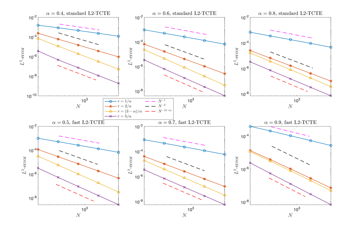
Figure 1: (Example 4.1) Maximum $L^{2}$-errors ${\tt err}_{\rm max}$. Top: Standard L2-TCTE method on the graded meshes with different $r$ and $N$ for $\alpha=0.4$, $\alpha=0.6$, $\alpha=0.8$ from left to right. Bottom: Fast L2-TCTE method on the graded meshes with different $r$ and $N$ for $\alpha=0.5$, $\alpha=0.7$, $\alpha=0.9$ from left to right.

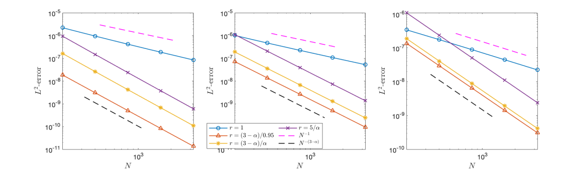
Figure 2: (Example 4.1) Final-time $L^{2}$-errors ${\tt err}_{T}$ for the standard L2-TCTE method on the graded meshes with different $r$ and $N$ for $\alpha=0.4$, $\alpha=0.6$, $\alpha=0.8$ from left to right.

Denote the $L^{2}$-error at time $t_{k}$ by

$${\tt err}_{t_{k}}\coloneqq\|u(t_{k})-u^{k}\|.$$

We show the differences of pointwise $L^{2}$-errors,

$${\tt err}_{t_{k}}^{\rm GK}-{\tt err}_{t_{k}}^{\rm TCTE},$$

between using the standard L2-Gauss and standard L2-TCTE methods (the left-hand side of Figure 3) and the fast L2-Gauss and fast L2-TCTE methods (the right-hand side of Figure 3). It is observed that the differences are almost the machine error, which verifies the accuracy of our method. However, we shall mention that the Gauss–Kronrod quadrature method could be much more expensive than our TCTE method, which will be discussed in the next subsection.

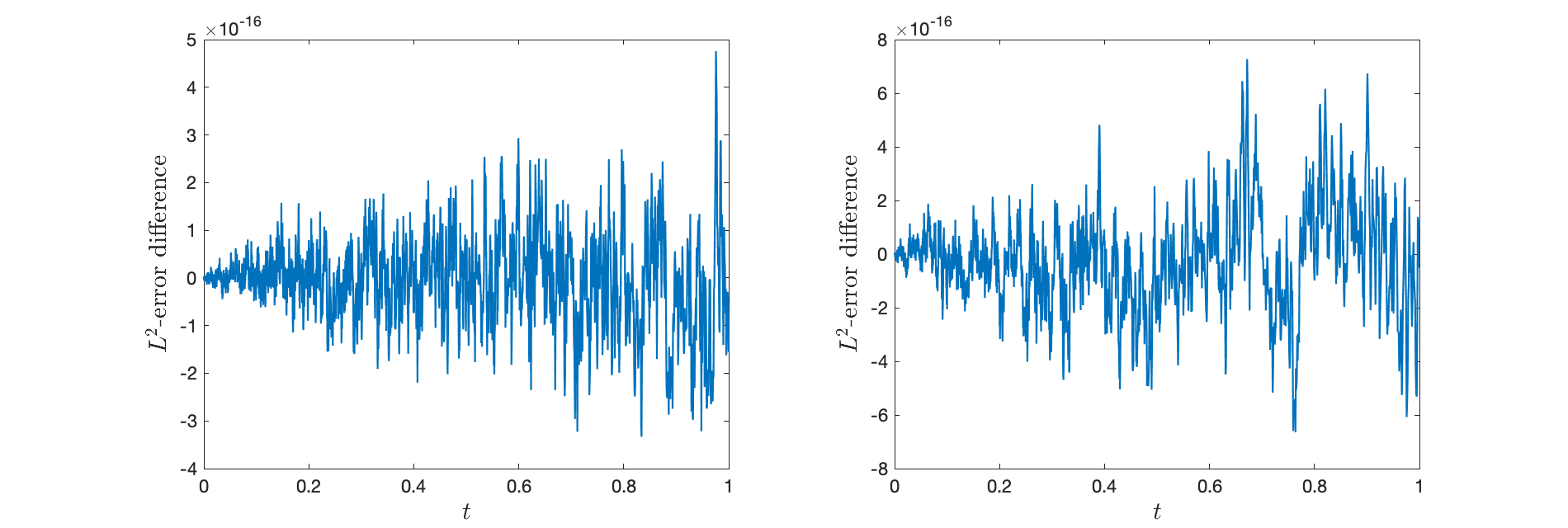
Figure 3: (Example 4.1) Pointwise $L^{2}$-error differences between the Gauss–Kronrod quadrature method and the TCTE method w.r.t. $t$, where $T=1$ and $N=3200$. Left: Standard L2 method with $\alpha=0.6$ and $r=(3-\alpha)/0.95$. Right: Fast L2 method with $\alpha=0.7$ and $r=(3-\alpha)/\alpha$.

4.2 High efficiency of TCTE method

Example 4.2.

Consider the subdiffusion equation (4.1) in $\Omega=[-1,1]^{2}$ with $T=10$ and $f(t,x,y)=\Gamma(1+\alpha)(x^{2}-1)(y^{2}-1)-2t^{\alpha}(x^{2}+y^{2}-2)$, whose exact solution is $u(t,x,y)=t^{\alpha}(x^{2}-1)(y^{2}-1)$.

In this example, we set the final time of SOE $T_{\rm soe}=T$, the SOE tolerance $\varepsilon=1\text{e-12}$, the cut-off time $\Delta t=\tau_{2}$ in SOE approximations; see [5, 17]. Since the exact solution is polynomial of degree 2 in $x$ and $y$ direction, we use the spectral collocation method in space with $5^{2}$ Chebyshev–Gauss–Lobatto points so that the error caused by space discretization is negligible.

Maximum error and $L^{2}$-error at final time $T=10$ and CPU time (in seconds) for the standard L2-Gauss, standard L2-TCTE, fast L2-Gauss and fast L2-TCTE methods are given in Table 2, where $\alpha=0.6$ and $r=(3-\alpha)/\alpha$. We observe that the CPU time of the fast L2 scheme increases approximately linearly w.r.t. $N$, while the CPU time of the standard L2 scheme increases approximately quadratically. Optimal convergence rate $3-\alpha$ is achieved, which is consistent with the convergence result [10, Theorem 5.2]. For a fixed $N$, the errors of the standard L2-Gauss and L2-TCTE methods are almost the same in sense that their differences are approximately the machine error. Influenced by the chosen SOE tolerance error $\varepsilon=1\text{e-12}$, the differences of $L^{2}$-errors between the standard and fast methods are about $\varepsilon$.

As one can see, when $N=32000$, the standard L2-TCTE method about 91 times faster than the standard L2-Gauss method, while the fast L2-TCTE method is about 308 times faster than the fast L2-Gauss method in this example.

Table 2: (Example 4.2) Maximum errors, final-time errors, and CPU times (in seconds) computed by standard L2-Gauss, standard L2-TCTE, fast L2-Gauss and fast L2-TCTE methods with $\alpha=0.6$, $r=(3-\alpha)/\alpha$ and $T=10$ for different numbers of time steps.

  $N=2000$ $N=4000$ $N=8000$ $N=16000$ $N=32000$ standard L2-Gauss ${\tt err}_{\rm max}$ 3.8628e-7 7.3187e-8 1.3866e-8 2.6271e-9 4.9776e-10 – 2.4000 2.4000 2.4000 2.4000 ${\tt err}_{T}$ 3.1934e-9 6.0409e-10 1.1434e-10 2.1654e-11 4.0991e-12 – 2.4023 2.4013 2.4007 2.4013 CPU time 9.5653e+2 3.8583e+3 1.5218e+4 6.0095e+4 2.4060e+5 standard L2-TCTE ${\tt err}_{\rm max}$ 3.8628e-7 7.3187e-8 1.3866e-8 2.6271e-9 4.9776e-10 – 2.4000 2.4000 2.4000 2.4000 ${\tt err}_{T}$ 3.1934e-9 6.0409e-10 1.1434e-10 2.1654e-11 4.0998e-12 – 2.4023 2.4013 2.4007 2.4010 CPU time 8.5312 35.3594 147.7656 623.7969 2639.0823 fast L2-Gauss ${\tt err}_{\rm max}$ 3.8628e-7 7.3187e-8 1.3866e-8 2.6271e-9 4.9776e-10 – 2.4000 2.4000 2.4000 2.4000 ${\tt err}_{T}$ 3.1935e-9 6.0417e-10 1.1442e-10 2.1731e-11 4.1806e-12 – 2.4021 2.4005 2.3966 2.3779 CPU time 134.0000 307.0156 634.1875 1322.6875 2810.9687 fast L2-TCTE ${\tt err}_{\rm max}$ 3.8628e-7 7.3187e-8 1.3866e-8 2.6271e-9 4.9776e-10 – 2.4000 2.4000 2.4000 2.4000 ${\tt err}_{T}$ 3.1935e-9 6.0417e-10 1.1442e-10 2.1730e-11 4.1803e-12 – 2.4021 2.4005 2.3967 2.3780 CPU time 0.4375 0.9062 1.9688 4.2500 9.1250  

4.3 Long time simulation

For simplicity, we still consider Example 4.2 but replacing the final time $T=10$ with $T=1000$. We set the final time of SOE $T_{\rm soe}=T$, the SOE tolerance $\varepsilon=1\text{e-14}$, the SOE cut-off time $\Delta t=\tau_{2}$, and the grading parameter $r=(3-\alpha)/\alpha$. Still, $5^{2}$ Chebyshev–Gauss–Lobatto points are used in the spectral collocation method for spatial discretization. The fast L2-TCTE method is adopted for this long time simulation.

In Table 3, the maximum $L^{2}$-errors, the final-time $L^{2}$-errors, the convergence rates, and the CPU times are reported. We can observe that the convergence rates are optimal and what’s more important, the CUP time is not large even for very large number of time steps ($N$ is larger than one hundred of thousands). To the best of knowledge, there are no existing simulations in literatures with more than $10^{6}$ time steps. The high efficiency of our TCTE method helps to achieve this.

Table 3: (Example 4.2) Maximum errors, final-time errors, and CPU times (in seconds) computed by fast L2-TCTE method with $r=(3-\alpha)/\alpha$ and $T=1000$ for different numbers of time steps.

  $N=8000$ $N=16000$ $N=32000$ $N=64000$ $N=128000$ $\alpha=0.4$ ${\tt err}_{\rm max}$ 7.9773e-8 1.3157e-8 2.1702e-9 3.5795e-10 5.9040e-11 – 2.6000 2.6000 2.6000 2.6000 ${\tt err}_{T}$ 4.3198e-11 7.0758e-12 1.1718e-12 1.9549e-13 4.2172e-14 – 2.6100 2.5941 2.5836 2.2127 CPU time 4.3906 6.8438 13.5156 27.9844 58.1406 $\alpha=0.6$ ${\tt err}_{\rm max}$ 2.1976e-7 4.1638e-8 7.8889e-9 1.4946e-9 2.8318e-10 – 2.4000 2.4000 2.4000 2.4000 ${\tt err}_{T}$ 1.1247e-10 2.1314e-11 4.0756e-12 7.6765e-13 1.3773e-13 – 2.3998 2.3867 2.4085 2.4785 CPU time 2.2031 4.8281 10.1094 21.5000 46.1406 $\alpha=0.8$ ${\tt err}_{\rm max}$ 1.3302e-6 2.9038e-7 6.3250e-8 1.3768e-8 2.9966e-9 – 2.1956 2.1988 2.1997 2.1999 ${\tt err}_{T}$ 2.2127e-10 4.8295e-11 1.0636e-11 2.4319e-12 5.7001e-13 – 2.1959 2.1829 2.1288 2.0930 CPU time 2.0000 4.0312 8.9219 18.7812 40.8125  

5 Conclusion

In this work, to handle the roundoff error problems in L2-type method, we reformulate the standard and fast L2 coefficients, provide the threshold conditions on $\delta$-cancellation, and propose the Taylor expansions to avoid $\delta$-cancellation when the threshold conditions are not satisfied. Numerical experiments show the high accuracy and efficiency of our proposed TCTE method. In particular, the fast L2-TCTE method can complete long time simulations with hundreds of thousands of time steps in one minute.

References

- [1] Anatoly A Alikhanov. A new difference scheme for the time fractional diffusion equation. Journal of Computational Physics, 280:424–438, 2015.
- [2] Michele Caputo. Linear models of dissipation whose Q is almost frequency independent–II. Geophysical Journal International, 13(5):529–539, 1967.
- [3] Hu Chen and Martin Stynes. Error analysis of a second-order method on fitted meshes for a time-fractional diffusion problem. Journal of Scientific Computing, 79(1):624–647, 2019.
- [4] Guang-hua Gao, Zhi-zhong Sun, and Hong-wei Zhang. A new fractional numerical differentiation formula to approximate the Caputo fractional derivative and its applications. Journal of Computational Physics, 259:33–50, 2014.
- [5] Shidong Jiang, Jiwei Zhang, Qian Zhang, and Zhimin Zhang. Fast evaluation of the Caputo fractional derivative and its applications to fractional diffusion equations. Communications in Computational Physics, 21(3):650–678, 2017.
- [6] Bangti Jin, Buyang Li, and Zhi Zhou. Correction of high-order BDF convolution quadrature for fractional evolution equations. SIAM Journal on Scientific Computing, 39(6):A3129–A3152, 2017.
- [7] Bangti Jin, Buyang Li, and Zhi Zhou. Subdiffusion with time-dependent coefficients: improved regularity and second-order time stepping. Numerische Mathematik, 145(4):883–913, 2020.
- [8] Rihuan Ke, Michael K Ng, and Hai-Wei Sun. A fast direct method for block triangular Toeplitz-like with tri-diagonal block systems from time-fractional partial differential equations. Journal of Computational Physics, 303:203–211, 2015.
- [9] Natalia Kopteva. Error analysis of the L1 method on graded and uniform meshes for a fractional-derivative problem in two and three dimensions. Mathematics of Computation, 88(319):2135–2155, 2019.
- [10] Natalia Kopteva. Error analysis of an L2-type method on graded meshes for a fractional-order parabolic problem. Mathematics of Computation, 90(327):19–40, 2021.
- [11] Natalia Kopteva and Xiangyun Meng. Error analysis for a fractional-derivative parabolic problem on quasi-graded meshes using barrier functions. SIAM Journal on Numerical Analysis, 58(2):1217–1238, 2020.
- [12] TAM Langlands and Bruce I Henry. The accuracy and stability of an implicit solution method for the fractional diffusion equation. Journal of Computational Physics, 205(2):719–736, 2005.
- [13] Xin Li, Hong-lin Liao, and Luming Zhang. A second-order fast compact scheme with unequal time-steps for subdiffusion problems. Numerical Algorithms, 86(3):1011–1039, 2021.
- [14] Hong-lin Liao, Dongfang Li, and Jiwei Zhang. Sharp error estimate of the nonuniform L1 formula for linear reaction-subdiffusion equations. SIAM Journal on Numerical Analysis, 56(2):1112–1133, 2018.
- [15] Hong-lin Liao, William McLean, and Jiwei Zhang. A Discrete Grönwall Inequality with Applications to Numerical Schemes for Subdiffusion Problems. SIAM Journal on Numerical Analysis, 57(1):218–237, 2019.
- [16] Hong-Lin Liao, William McLean, and Jiwei Zhang. A second-order scheme with nonuniform time steps for a linear reaction-subdiffusion problem. Communications in Computational Physics, 30(2):567–601, 2021.
- [17] Hong-lin Liao, Yonggui Yan, and Jiwei Zhang. Unconditional convergence of a fast two-level linearized algorithm for semilinear subdiffusion equations. Journal of Scientific Computing, 80(1):1–25, 2019.
- [18] Nan Liu, Yanping Chen, Jiwei Zhang, and Yanmin Zhao. Unconditionally optimal -error estimate of a fast nonuniform L2-1 scheme for nonlinear subdiffusion equations. Numerical Algorithms, pages 1–23, 2022.
- [19] Chunwan Lv and Chuanju Xu. Error analysis of a high order method for time-fractional diffusion equations. SIAM Journal on Scientific Computing, 38(5):A2699–A2724, 2016.
- [20] Kassem Mustapha, Basheer Abdallah, and Khaled M Furati. A discontinuous Petrov–Galerkin method for time-fractional diffusion equations. SIAM Journal on Numerical Analysis, 52(5):2512–2529, 2014.
- [21] Chaoyu Quan and Boyi Wang. Energy stable L2 schemes for time-fractional phase-field equations. Journal of Computational Physics, 458:111085, 2022.
- [22] Chaoyu Quan and Xu Wu. -stability of an L2-type method on general nonuniform meshes for subdiffusion equation. arXiv preprint arXiv:2205.06060, 2022.
- [23] Chaoyu Quan and Xu Wu. On stability and convergence of L2-1σ method on general nonuniform meshes for subdiffusion equation. arXiv preprint arXiv:2208.01384, 2022.
- [24] Chaoyu Quan, Xu Wu, and Jiang Yang. Long time -stability of fast L2-1σ method on general nonuniform meshes for subdiffusion equations. arXiv preprint arXiv:2212.00453, 2022.
- [25] Jie Shen, Tao Tang, and Li-Lian Wang. Spectral methods: algorithms, analysis and applications, volume 41. Springer Science & Business Media, 2011.
- [26] Martin Stynes, Eugene O’Riordan, and José Luis Gracia. Error analysis of a finite difference method on graded meshes for a time-fractional diffusion equation. SIAM Journal on Numerical Analysis, 55(2):1057–1079, 2017.
- [27] Zhi-zhong Sun and Xiaonan Wu. A fully discrete difference scheme for a diffusion-wave system. Applied Numerical Mathematics, 56(2):193–209, 2006.
- [28] Lloyd N Trefethen. Spectral methods in MATLAB. SIAM, 2000.
- [29] Hongyi Zhu and Chuanju Xu. A fast high order method for the time-fractional diffusion equation. SIAM Journal on Numerical Analysis, 57(6):2829–2849, 2019.