An Efficient Framework for Monitoring Subgroup Performance of Machine Learning Systems

Abstract

Monitoring machine learning systems post deployment is critical to ensure the reliability of the systems. Particularly importance is the problem of monitoring the performance of machine learning systems across all the data subgroups (subpopulations). In practice, this process could be prohibitively expensive as the number of data subgroups grows exponentially with the number of input features, and the process of labelling data to evaluate each subgroup’s performance is costly. In this paper, we propose an efficient framework for monitoring subgroup performance of machine learning systems. Specifically, we aim to find the data subgroup with the worst performance using a limited number of labeled data. We mathematically formulate this problem as an optimization problem with an expensive black-box objective function, and then suggest to use Bayesian optimization to solve this problem. Our experimental results on various real-world datasets and machine learning systems show that our proposed framework can retrieve the worst-performing data subgroup effectively and efficiently.

1 Introduction

Supervised machine learning (ML) systems are increasingly deployed in critical application domains but there is no guarantee that these systems will continue to perform well after deployment  [25]. Monitoring the performance of ML systems is thus crucial to prevent potential failures that may cause severe unintended consequences [8, 27]. Particularly importance is to monitor the performance of ML systems across all the data subgroups so as to discover the scenarios when the systems may show anomalous or faulty behaviours [27]. In practice, there have been various issues reported regarding the malicious performance of well-known ML systems on some particular data subgroups. For example, researchers have noted that in COMPAS [15], an ML system used across US courtrooms to predict future crimes, females who initially committed misdemeanors have their recidivism risk significantly over-estimated for half of the COMPAS risk groups [30]. Another example is that various commercial facial detection algorithms have been shown to perform significantly different across different data subgroups of races and genders with a worse performance on females with darker skins [2]. In practice, it is recognized that organizations often want to understand the performance of the ML systems on different demographic data subgroups, customer segments, etc. [27]. Therefore, it is important to monitor the performance of an ML system across the data subgroups (subpopulations).

Existing literature tackles this problem by focusing on some limited pre-defined data subgroups (e.g., gender and race). However, this does not include all the possible subgroups, and therefore, important defective subgroups might not be discovered. In this work, we aim to monitor the ML systems’ performance across all the possible data subgroups. In particular, we aim to find the data subgroup where an ML system performs the worst. An exhaustive search across all the subgroups could be prohibitively expensive, and in many cases, is impossible. The reason is that evaluating the performance of an ML system on a data subgroup requires the collection of an amount of labelled data corresponding to that subgroup. For example, to evaluate the performance of an ML system for the data subgroup female + black + married, a set of labelled data with input attributes female, black, and married need to be collected. However, the number of possible data subgroups scales exponentially with the number of input attributes (to be used to create subgroups), and thus the amount of labelled data to be collected could be exploded if an exhaustive search is employed. For a dataset with $n$ input attributes (to be used to create subgroups) and each attribute has $m_{i}$ distinct values, the number of possible data subgroups is $\prod_{i=1}^{n}m_{i}$. If it is required to collect $K$ labelled data points to estimate the performance of a data subgroup, then in total, $K\prod_{i=1}^{n}m_{i}$ data points need to be labelled, which is expensive and could be impossible in many situations.

In this paper, we propose an efficient framework that can find the worst-performing data subgroup with a minimal number of labelled data. We first formulate the problem as an optimization problem with an expensive black-box objective function. We then suggest to use Bayesian Optimization (BO), a powerful sequential global optimization technique, so as to find the worst-performing data subgroup efficiently. The key idea of BO is to train a surrogate model from an initial labelled dataset, construct an acquisition function from this surrogate model, and use this function to select the most informative data subgroup(s) that can help to find the worst-performing subgroup most efficiently. Our framework can work with various types of supervised ML systems, e.g. classifier and regressor, and can also work with different performance metrics such as accuracy, mean square error, precision, recall.

In summary, our contributions are:

1. A generic and efficient framework for monitoring the subgroup performance of ML systems;

2. An effective technique that can help to find the worst-performing data subgroup using a minimal number of labelled data;

3. A set of experiments to demonstrate the efficacy of our proposed framework.

Related Work

There have been various research works tackling the problem of assessing or monitoring the subgroup performance of an ML system, however, their settings are generally different compared to ours. Please refer to Section A.1 in the Appendix for more details.

2 An Efficient Framework for Monitoring Subgroup Performance

In this section, we present our proposed framework for monitoring subgroup performance of an ML system. An overview of our proposed framework is shown in Figure 1.

2.1 Formulating the Subgroup Monitoring Problem

Let us denote an individual input data and its ground-truth as $((x,x^{\prime}),y_{x,x^{\prime}})$ where $x\in\mathcal{X}$ denotes the attributes that are used to construct the data subgroups, $x^{\prime}\in\mathcal{X}^{\prime}$ as the attributes of non-interest, and $y_{x,x^{\prime}}$ as the corresponding ground-truth of $(x,x^{\prime})$. For example, for a problem of using census data of a person to predict their income, one can set the attributes $x$ to be gender, race, relationship, age whilst other attributes can be set as attributes of non-interest $x^{\prime}$. The choice of attributes to be used to construct the subgroups depends on the users, in particular, it depends on which data segments the users want to monitor. Given an ML system $C$, let us denote $C(x,x^{\prime})$ as the prediction of $C$ for an input $(x,x^{\prime})$. The performance value of the system $C$ with a metric $M$ can then be expressed as,

$$M(C)=M(C_{\mathcal{X},\mathcal{X}^{\prime}},\mathcal{Y}_{\mathcal{X},\mathcal{X}^{\prime}}),$$

where $C_{\mathcal{X},\mathcal{X}^{\prime}}=\{C(x,x^{\prime})\}_{x\in\mathcal{X},x^{\prime}\in\mathcal{X}^{\prime}}$, $\mathcal{Y}_{\mathcal{X},\mathcal{X}^{\prime}}=\{y_{x,x^{\prime}}\}_{x\in\mathcal{X},x^{\prime}\in\mathcal{X}^{\prime}}$. Then the performance value of the ML system $C$ w.r.t. a data subgroup $x$ can be computed as,

$$M_{x}(C)=M(C_{x,\mathcal{X}^{\prime}},\mathcal{Y}_{x,\mathcal{X}^{\prime}}).$$

The problem of finding the worst-performing data subgroup becomes the problem of finding $x^{*}$:

$$x^{*}=\operatorname*{arg\,min}\nolimits_{x\in\mathcal{X}}M_{x}(C).$$ (1)

As discussed in Section 1, computing $M_{x}(C)$ for each data subgroup $x$ is expensive, therefore, it is generally impossible to exhaustively search for $x^{*}$. In this paper, we aim to solve the optimization problem in Eq. (1) in an efficient manner, i.e., using a minimal number of evaluations of $M_{x}(C)$.

2.2 An Efficient Subgroup Searching Methodology

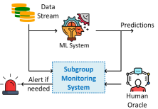
Figure 1: Left: The subgroup performance monitoring workflow; the monitoring system takes the data stream, the ML systems’ predictions, and a human oracle as inputs, and outputs the worst-performing data subgroup that can alert users regarding the quality of the ML system. Right: The detailed implementation of our proposed subgroup performance monitoring framework based on BO method.

To solve the optimization problem in Eq. (1) in an efficient manner, we propose to use Bayesian Optimization (BO) technique [14, 13, 28, 26]. BO is a powerful optimization method to find the global optimum of an expensive black-box objective function by sequential queries. Applying BO to solve the problem in Eq. (1) can be done as follows.

Firstly, an initial dataset $D_{0}=\{(x_{i},M_{x_{i}}(C))\}_{i=1}^{N_{0}}$ is constructed from a number of data subgroups $\{x_{i}\}_{i=1}^{N_{0}}$ and their corresponding performance values $\{M_{x_{i}}(C)\}_{i=1}^{N_{0}}$. Secondly, a surrogate model is trained on this initial dataset to approximate the behaviour of the performance function $M_{x}(C)$. Thirdly, an acquisition function is constructed from this surrogate model to suggest the next most informative data subgroup to be evaluated so as to find the worst-performing subgroup $x^{*}$ fastest. The ML system’s performance is then evaluated at this data subgroup and the data pair is then added to $D_{0}$. The process is conducted repeatedly until the labelling budget is depleted. The worst-performing subgroup $\hat{x}^{*}$ is then chosen as the worst-performing subgroup from the labelled dataset $D_{T}$ obtained after the BO process, i.e., $\hat{x}^{*}=\operatorname*{arg\,min}_{x\in D_{T}}M_{x}(C)$.

In the BO technique, there are various common choices of surrogate models including the Gaussian Process (GP) [23], the random forest [12, 1], the neural network [29]. In this work, we use a GP as the surrogate model of the BO process as GP has been shown to be effective in many practical scenarios [28, 26]. Note that, in the subgroup performance monitoring problem, the data subgroups $x$ are categorical variables, so we use the corresponding BO technique for categorical variables. In particular, the categorical variables are one-hot encoded, so that they can be treated as continuous variables, and then the standard continuous BO process is performed on the transformed variables. Finally, we use the Expected Improvement (EI) [19] as the acquisition function as it is one of the most effective and well-studied acquisition functions in the BO literature [26].

3 Experimental Results

In this section, we describe in details the experimental evaluation of our proposed framework. Our experiments aim to answer the question of whether our proposed framework can find the worst-performing data subgroup efficiently.

Datasets

We evaluate our proposed framework using two real-world datasets from the UC Irvine (UCI) Data Repository. The first dataset is the Adult dataset [17]. Each record in this dataset describes the census data of a person and the goal is to predict whether the income of this person exceeds 50,000 USD per year. We choose the subgroup attributes to be age, race, gender and relationship. The second dataset we use for evaluation is the Bike Sharing dataset [5]. This dataset contains the hourly count of rental bikes between years 2011 and 2012 in Capital bikeshare system with the corresponding weather and seasonal information. The goal is to predict the hourly count of rental bikes given a particular weather and seasonal information. For this dataset, we choose the subgroup attributes to be season, weather, hours, and working day.

Machine Learning Systems

We split each dataset into two parts: training and testing. We have two choices of training size: 1000 and 2000 data points, the rest of the data is the testing part. We train different ML systems on the training part and then use our proposed framework to find the worst-performing data subgroups of these ML systems on the test part. The Adult dataset corresponds to a classification problem, so we use Logistic Regression [3] and Gradient Boosting [7] as the ML systems, and the classification accuracy as the performance metric. The Bike Sharing dataset corresponds to a regression problem so we use Linear Regression [11] and Gradient Boosting [7] as the ML systems, and the mean square error as the performance metric. With two choices of training dataset size, we have in total four ML systems for each dataset. For each combination of dataset and ML system, we repeat the experiments 20 times with different split of training and testing parts, and report the means and standard errors of the worst subgroup performance found at each iteration.

Baselines

We compare our proposed framework with two baselines: Random Search (RS) and Exhaustive Search (ES). With RS, we randomly select a number of data subgroups, evaluate the ML system’s performance associated with these subgroups, and then retrieve the worst-performing subgroup. With ES, we construct all the possible valid data subgroups, sequentially evaluate the ML system’s performance of all the subgroups, and then retrieve the worst-performing subgroup.

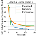
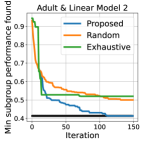
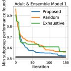
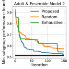
Figure 2: Results of the Adult dataset with different ML systems. Black lines are the true worst subgroup performance. Coloured lines are the worst subgroup performance found by the methods.

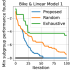
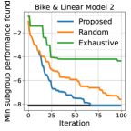
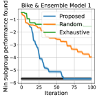
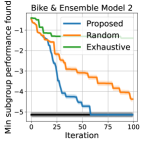
Figure 3: Results of the Bike Sharing dataset with different ML systems. Black lines are the true worst subgroup performance. Coloured lines are the worst subgroup performance found by the methods.

In Figures 2 and 3, we show the experimental results of our proposed method and baseline methods for the Adult and Bike Sharing datasets, respectively. It can be clearly seen that our proposed method can find the worst-performing data subgroup much faster compared to the baseline methods. For the Adult dataset, our proposed method can find the worst-performing subgroup after only around 100 iterations (i.e., 100 subgroup performance evaluations) whilst other methods takes much more iterations to find this subgroup. Similarly, for the Bike Sharing dataset, our proposed method can find the worst subgroup within 50-70 iterations, which is much faster compared to other baseline methods.

4 Conclusion

In this paper, we have proposed a framework for efficiently monitoring the performance of an ML system across all the data subgroups. In particular, we aim to find the data subgroup with the worst performance. Our proposed framework is data-efficient as it requires a minimal amount of labeled data, and generic as it can be applied to various types of ML systems and performance metrics. Our experimental results on two real-world datasets and various types of ML systems confirm the effectiveness of our proposed framework.

Appendix A Appendix

A.1 Related Work

There are various works targeting the problem of detecting the bad performance of an ML system on some data subgroups, especially in the context of evaluating the biasness of an ML system, for example, [4, 6, 20]. However, most of these work only aim to assess the performance of ML systems on some pre-defined data subgroups such as race, gender. Our work, on the other hand, assesses the performance of an ML system across all the data subgroups.

Directly related to our work, there are some works targeting the problem of assessing the performance of an ML system across all the data subgroups, however, these work can only work on a limited types of ML system (e.g., binary classifiers), and they do not target the problem of reducing the cost of labelling data. The work in [16] suggests considering the fairness statistical notions via a large number of subgroups. However, this work only considers the binary classifiers, on the other hand, our proposed framework can work with different types of ML systems including multi-class classifiers and regressors. The paper by Zhang and Neil [30] presents a subset scan method to detect if a probabilistic binary classifier has statistically significant bias over or under predicting the risk for some subgroups and identify the characteristics of this subgroup. However, similar to [16], this work also only works for binary classifiers, and it also does not focus on the problem of reducing the cost of labelling data. The work in [21] presented a method for finding data subgroups that behave differently from the overall dataset. However, the method does not tackle the problem of expensive labelled data as our proposed framework.

There are works targeting the problem of monitoring ML systems [8], but this work do not care about the performance of the ML systems across all the data subgroups. Finally, there are works that aim to test the performance of an ML system in a data-efficient manner [25, 9, 10, 18], however, these works also do not care about the performance across the data subgroups.

A.2 Background

Bayesian Optimization

Bayesian optimization is a powerful optimization method to find the global optimum of an unknown objective function $f(x)$ by sequential queries [14, 13, 28, 26]. First, at time $t$, a surrogate model is used to approximate the behaviour of $f(x)$ using all the current observed data $D_{t-1}=\{(x_{i},y_{i})\}^{n}_{i=1},y_{i}=f(x_{i})+\zeta_{i}$, where $\zeta_{i}\sim\mathcal{N}(0,\sigma^{2})$ is the noise. Second, an acquisition function is constructed from the surrogate model that suggests the next point $x_{itr}$ to be evaluated. The objective function is then evaluated at $x_{itr}$ and the new data point $(x_{itr},y_{itr})$ is added to $D_{t-1}$. These steps are conducted in an iterative manner to get the best estimate of the global optimum.

Gaussian Process

A GP defines a probability distribution over functions $f$ under the assumption that any finite subset $\{(\mathbf{x}_{i},f(\mathbf{x}_{i})\}$ follows a normal distribution [24]. Formally, a GP is defined as $f(\mathbf{x})\sim\text{GP}\left(\mu\left(\mathbf{x}\right),k\left(\mathbf{x},\mathbf{x}^{\prime}\right)\right)$, where $\mu(\mathbf{x})=\mathbb{E}\left[f\left(\mathbf{x}\right)\right]$ is the mean function and $k(\mathbf{x},\mathbf{x}^{\prime})=\mathbb{E}\left[(f\left(\mathbf{x}\right)-\mu\left(\mathbf{x}\right))(f\left(\mathbf{x}^{\prime}\right)-\mu\left(\mathbf{x}^{\prime}\right))^{T}\right]$ is the covariance function [24].

Assuming a zero mean prior $m(\mathbf{x})=0$ for simplicity, we have the joint multivariate Gaussian distribution between the observed point $f$ and a new data point $\mathbf{x}_{\text{new}},f_{\text{new}}=f\left(\mathbf{x}_{\text{new}}\right)$ as follows,

$$\left[\begin{array}[]{c}\boldsymbol{f}\\ f_{\text{new}}\end{array}\right] \sim\mathcal{N}\left(0,\left[\begin{array}[]{cc}\mathbf{K}&\mathbf{k}_{\text{new}}^{T}\\ \mathbf{k}_{\text{new}}&k_{\text{new}}\end{array}\right]\right),$$ (6)

where $k_{\text{new}}=k\left(\mathbf{x}_{\text{new}},\mathbf{x}_{\text{new}}\right)$, $\mathbf{k}_{\text{new}}=[k\left(\mathbf{x}_{\text{new}},\mathbf{x}_{i}\right)]_{\forall i\leq N}$ and $\mathbf{K}=\left[k\left(\mathbf{x}_{i},\mathbf{x}_{j}\right)\right]_{\forall i,j\leq N}$. Combining Eq. (6) with the fact that $p\left(f_{\text{new}}\mid\boldsymbol{f}\right)$ follows a univariate Gaussian distribution $\mathcal{N}\left(\mu\left(\mathbf{x}_{\text{new}}\right),\sigma^{2}\left(\mathbf{x}_{\text{new}}\right)\right)$, the GP posterior mean and variance at the data point $\mathbf{x}_{\text{new}}$ can be computed as,

$$\mu\left(\mathbf{x}_{\text{new}}\right)= \mathbf{k}_{\text{new}}\left[\mathbf{K}+\sigma^{2}\mathbf{I}\right]^{-1}\mathbf{y},$$

$$\sigma^{2}\left(\mathbf{x}_{\text{new}}\right)= k_{\text{new}}-\mathbf{k}_{\text{new}}\left[\mathbf{K}+\sigma^{2}\mathbf{I}\right]^{-1}\mathbf{k}_{\text{new}}^{T}.$$

As GPs give full uncertainty information with any prediction, they provide a flexible nonparametric prior for Bayesian optimization. We refer the interested readers to [24] for further details on GPs.

A.3 Experimental Setup

Datasets

We evaluate our proposed framework using two real-world datasets from the UC Irvine (UCI) Data Repository. The first dataset is the Adult dataset [17]. Each record in this dataset describes the census data of a person (e.g., age, race, gender, relationship, workclass, education), and the goal is to predict whether the income of this person exceeds 50,000 USD per year. We choose the subgroup attributes to be age, race, gender and relationship. Note that for the age attribute, we group the values to be within 6 distinct values representing people with ages less than 20, from 20 to 30, …, 50 to 60, and more than 60. The second dataset we use for evaluation is the Bike Sharing dataset [5]. This dataset contains the hourly count of rental bikes between years 2011 and 2012 in Capital bikeshare system with the corresponding weather and seasonal information. The goal is to predict the hourly count of rental bikes given a particular weather and seasonal information. For this dataset, we choose the subgroup attributes to be season, weather, hours, and working day. For the hour attribute, we group the values to be within 5 distinct values representing early morning, morning, afternoon, evening and midnight.

Machine Learning Systems

We split each dataset into two parts: training and testing. We have two choices of training size: 1000 and 2000 data points, the rest of the data is the testing part. We train different ML systems on the training parts and then use our proposed framework to find the worst-performing subgroup of these ML systems on the test part. In particular, for each subgroup $x$, we compute the metric value $M_{x}(C)$ by collecting the labelled data points in the dataset according to this subgroup. For classification problems (Adult and Bank datasets), we use the Logistic Regression and the Gradient Boosting as the ML systems. For the regression problem (Bike Sharing dataset), we use the Linear Regression and Gradient Boosting as the ML systems. All the ML systems are implemented using sklearn [22] with default settings. For each ML system, we repeat the experiments 20 times with different split of training and testing parts.

Baselines

We compare our proposed framework with two baselines: Random Search and Exhaustive Search. With Random Search, we randomly select a number of subgroups, evaluate the ML system’s performance associated with these subgroups, and then retrieve the worst-performing subgroup based on these performance values. With Exhaustive Search, we construct all the possible valid subgroups, and then sequentially evaluate the ML system’s performance on each subgroup until the labelling budget is depleted. We then retrieve the worst-performing subgroup based on the evaluated performance values.

References

- [1] Leo Breiman. Random forests. Machine Learning, 45(1):5–32, 2001.
- [2] Joy Buolamwini and Timnit Gebru. Gender shades: Intersectional accuracy disparities in commercial gender classification. In Conference on Fairness, Accountability and Transparency (FAT), volume 81 of Proceedings of Machine Learning Research, pages 77–91. PMLR, 2018.
- [3] David R Cox. The regression analysis of binary sequences. Journal of the Royal Statistical Society: Series B (Methodological), 20(2):215–232, 1958.
- [4] Cynthia Dwork and Christina Ilvento. Group fairness under composition. In Proceedings of the 2018 Conference on Fairness, Accountability, and Transparency (FAT* 2018), 2018.
- [5] Hadi Fanaee-T and Joao Gama. Event labeling combining ensemble detectors and background knowledge. Progress in Artificial Intelligence, pages 1–15, 2013.
- [6] James R. Foulds, Rashidul Islam, Kamrun Naher Keya, and Shimei Pan. An intersectional definition of fairness. In 36th IEEE International Conference on Data Engineering (ICDE), pages 1918–1921. IEEE, 2020.
- [7] Jerome H. Friedman. Stochastic gradient boosting. Computational Statistics & Data Analysis, 38(4):367–378, 2002. Nonlinear Methods and Data Mining.
- [8] Tony Ginart, Martin Jinye Zhang, and James Zou. Mldemon: Deployment monitoring for machine learning systems. In Gustau Camps-Valls, Francisco J. R. Ruiz, and Isabel Valera, editors, International Conference on Artificial Intelligence and Statistics (AISTATS), volume 151 of Proceedings of Machine Learning Research, pages 3962–3997. PMLR, 2022.
- [9] Shivapratap Gopakumar, Sunil Gupta, Santu Rana, Vu Nguyen, and Svetha Venkatesh. Algorithmic assurance: An active approach to algorithmic testing using bayesian optimisation. In Advances in Neural Information Processing Systems 31: Annual Conference on Neural Information Processing Systems (NeurIPS0, pages 5470–5478, 2018.
- [10] Huong Ha, Sunil Gupta, Santu Rana, and Svetha Venkatesh. ALT-MAS: A data-efficient framework for active testing of machine learning algorithms. CoRR, abs/2104.04999, 2021.
- [11] Trevor Hastie, Jerome H. Friedman, and Robert Tibshirani. The Elements of Statistical Learning: Data Mining, Inference, and Prediction. Springer Series in Statistics. Springer, 2001.
- [12] Frank Hutter, Holger H. Hoos, and Kevin Leyton-Brown. Sequential model-based optimization for general algorithm configuration. In Learning and Intelligent Optimization - 5th International Conference (LION), volume 6683 of Lecture Notes in Computer Science, pages 507–523. Springer, 2011.
- [13] Donald R. Jones. A taxonomy of global optimization methods based on response surfaces. Journal of Global Optimization, 21(4):345–383, 2001.
- [14] Donald R. Jones, Matthias Schonlau, and William J. Welch. Efficient global optimization of expensive black-box functions. Journal of Global Optimization, 13(4):455–492, 1998.
- [15] Surya Mattu Julia Angwin, Jeff Larson and Lauren Kirchner. Machine bias, 2016.
- [16] Michael J. Kearns, Seth Neel, Aaron Roth, and Zhiwei Steven Wu. Preventing fairness gerrymandering: Auditing and learning for subgroup fairness. In Proceedings of the 35th International Conference on Machine Learning (ICML), volume 80, pages 2569–2577. PMLR, 2018.
- [17] Ron Kohavi. Scaling up the accuracy of naive-bayes classifiers: A decision-tree hybrid. In Evangelos Simoudis, Jiawei Han, and Usama M. Fayyad, editors, Proceedings of the Second International Conference on Knowledge Discovery and Data Mining (KDD), pages 202–207. AAAI Press, 1996.
- [18] Jannik Kossen, Sebastian Farquhar, Yarin Gal, and Tom Rainforth. Active testing: Sample-efficient model evaluation. In Proceedings of the 38th International Conference on Machine Learning (ICML), volume 139 of Proceedings of Machine Learning Research, pages 5753–5763. PMLR, 2021.
- [19] Jonas Mockus. On bayesian methods for seeking the extremum. In Guri I. Marchuk, editor, Optimization Techniques IFIP Technical Conference Novosibirsk, July 1–7, 1974, pages 400–404, Berlin, Heidelberg, 1975. Springer Berlin Heidelberg.
- [20] Giulio Morina, Viktoriia Oliinyk, Julian Waton, Ines Marusic, and Konstantinos Georgatzis. Auditing and achieving intersectional fairness in classification problems. CoRR, abs/1911.01468, 2019.
- [21] Eliana Pastor, Luca de Alfaro, and Elena Baralis. Identifying biased subgroups in ranking and classification. CoRR, abs/2108.07450, 2021.
- [22] Fabian Pedregosa, Gaël Varoquaux, Alexandre Gramfort, Vincent Michel, Bertrand Thirion, Olivier Grisel, Mathieu Blondel, Peter Prettenhofer, Ron Weiss, Vincent Dubourg, Jake VanderPlas, Alexandre Passos, David Cournapeau, Matthieu Brucher, Matthieu Perrot, and Edouard Duchesnay. Scikit-learn: Machine learning in Python. Journal of Machine Learning Research, 12:2825–2830, 2011.
- [23] Carl Edward Rasmussen and Christopher K. I. Williams. Gaussian processes for machine learning. MIT Press, 2006.
- [24] Carl Edward Rasmussen and Christopher KI Williams. Gaussian processes for machine learning. 2006.
- [25] Christoph Sawade, Niels Landwehr, Steffen Bickel, and Tobias Scheffer. Active risk estimation. In Proceedings of the 27th International Conference on Machine Learning (ICML), pages 951–958. Omnipress, 2010.
- [26] Bobak Shahriari, Kevin Swersky, Ziyu Wang, Ryan P. Adams, and Nando de Freitas. Taking the human out of the loop: A review of bayesian optimization. Proc. IEEE, 104(1):148–175, 2016.
- [27] Shreya Shankar, Rolando Garcia, Joseph M. Hellerstein, and Aditya G. Parameswaran. Operationalizing machine learning: An interview study. CoRR, abs/2209.09125, 2022.
- [28] Jasper Snoek, Hugo Larochelle, and Ryan P. Adams. Practical bayesian optimization of machine learning algorithms. In Advances in Neural Information Processing Systems 25: 26th Annual Conference on Neural Information Processing Systems (NeurIPS), pages 2960–2968, 2012.
- [29] Jasper Snoek, Oren Rippel, Kevin Swersky, Ryan Kiros, Nadathur Satish, Narayanan Sundaram, Md. Mostofa Ali Patwary, Prabhat, and Ryan P. Adams. Scalable bayesian optimization using deep neural networks. In Proceedings of the 32nd International Conference on Machine Learning, (ICML), volume 37, pages 2171–2180. JMLR.org, 2015.
- [30] Zhe Zhang and Daniel B. Neill. Identifying significant predictive bias in classifiers. CoRR, abs/1611.08292, 2016.