Three Dimensional Simulations of Advective, Sub-Keplerian Accretion Flow onto Non-rotating Black Holes

Abstract

We study the time evolution of sub-Keplerian transonic accretion flow onto a non-rotating black hole using a three-dimensional, inviscid hydrodynamics simulation code. Prior two-dimensional simulations show that centrifugal barrier in the accreting matter may temporarily halt the nearly free-falling matter and produce a stable, geometrically thick disk which may contain turbulent eddies. Our goal in this work is to investigate whether the disk develops any instability because of this turbulence when we dynamically activate all three dimensions. We find that the disk remains stable and axisymmetric even close to the central black hole. However, if we explicitly apply non-axisymmetric azimuthal perturbation, the axisymmetric structure of the disk is destroyed and instability is developed.

1 Introduction

Presence of a dynamical, geometrically thick, optically slim, hot advective corona surrounding a black hole helps in explaining the time-variability of the observed radiations for several X-ray sources containing black holes (Cui et al., 1997; Chakrabarti & Manickam, 2000; Radhika et al., 2016; Patra et al., 2019; Shang et al., 2019; Mondal & Chakrabarti, 2021, and references therein). Theoretical solution of hybrid flow (Chakrabarti, 1989a) containing a standing shock self-consistently explains the origin of such a corona as the post-shock sub-Keplerian accreting matter (Chakrabarti & Titarchuk, 1995). Close to the compact objects, the centrifugal barrier of this low-angular momentum, super-sonic, advective flow causes it to pass through a shock-transition and subsequently, produce the toroidal corona which may launch jet as well. The shock surface forms the boundary layer of the corona (centrifugal pressure supported boundary layer or CENBOL, Chakrabarti & Titarchuk, 1995).

Since the conceptualization of the centrifugal pressure supported shock formation in the accretion flow (Chang & Ostriker, 1985; Fukue, 1987; Chakrabarti, 1989b), several numerical experiments have been performed to verify the formation and stability of this shock surface. To verify their conjectures, Chakrabarti and his collaborators initially performed several one and two-dimensional simulations using different types of simulation codes, such as smooth particle hydrodynamics (SPH) and schemes based on finite-difference method (Chakrabarti & Molteni, 1993; Molteni et al., 1994; Molteni et al., 1996b; Ryu et al., 1997). These works demonstrated excellent matching of the theoretical and numerical solutions. Additionally, the results demonstrate the stability of the shocks in the accretion flow. Different other groups also independently performed simulations of low angular momentum, advective accretion flow onto black holes (Hawley et al., 1984; Ryu et al., 1995) and found presence of shocks although, in some case, shocks were unstable and moved outside the computational domain.

The shocked accretion flow is further studied in presence of various dissipative effects such as viscosity, radiation etc. In presence of Compton cooling, the thermal pressure inside the torus reduces and the shock moves closer to the central object (Molteni et al., 1996a; Chakrabarti et al., 2004; Okuda et al., 2007; Garain et al., 2012, 2014). On the other hand, outward angular momentum transport through viscosity pushes the shock outward and the angular momentum of the post-shock flow tends to become Keplerian (Chakrabarti & Molteni, 1995; Lanzafame et al., 1998, 2008; Lee et al., 2016). In presence of both cooling and viscous transport, it possible to demonstrate the stable coexistence of both optically thick, geometrically thin Keplerian disk and optically thin, geometrically thick torus of sub-Keplerian matter(Giri & Chakrabarti, 2013; Giri et al., 2015). Numerical studies of magnetized sub-Keplerian matter accretion flow has also been performed to understand the effect of magnetic field on the shock and the resulting torus (Deb et al., 2017; Okuda et al., 2019; Garain et al., 2020; Singh et al., 2021). All these simulations are performed in two-dimensions (2D) under axi-symmetric assumptions.

Through all these simulations, it is demonstrated that stable shock formation is indeed possible under various conditions in low angular momentum matter accretion onto a black hole. Although the formation of standing shock solution is found to be the case in theoretical analysis or even one-dimensional (1D) numerical simulations (Chakrabarti & Molteni, 1993; Kim et al., 2017, 2019), in multi-dimensional simulations, the shock location is generally found be dynamic. The collision between the incoming matter and the bounced back matter from the centrifugal barrier makes the flow turbulent. Dynamic eddies are seen to be self-consistently formed inside the post-shock region. These eddies are either advected into the black hole or move away in vertical direction. It is also realized that presence of turbulence pressure push the shock away from their predicted location.

While axisymmetry is used in the above mentioned 2D simulations, there are a few 2D simulations which are performed on the equatorial plane (thin-disk approximation), to study shock stability against non-axisymmetric azimuthal perturbations (Molteni et al., 1999; Nagakura & Yamada, 2008, 2009). These simulations start with an initial steady state, axisymmetric standing shocked solution. Then, a very small perturbation (1% or less) in pressure or density is advected along with infalling matter from outer boundary. This perturbation is applied momentarily on a few azimuthal grids. After the flow settles down, it is found that such a small amount of non-axisymmetric perturbation produces a shock instability named as standing accretion shock instability (SASI) and makes the shock non-axisymmetric, even though the inner and outer boundary conditions of the simulation remain same as that of axisymmetric standing shock. However, the follow up investigations without thin disk approximation are not reported.

There are only a few simulations of low angular momentum accretion flow, where all the three dimensions (3D) are dynamically active. Majority of 3D simulations to study accretion onto black holes start from an initial equilibrium torus (Porth et al., 2019, and references therein). Initial angular momentum of matter inside such a torus is very high and hence, significant angular momentum transport is required to enable accretion of this matter onto black holes. Janiuk et al. (2008); Janiuk et al. (2009); Kurosawa & Proga (2009) studied the accretion of low angular momentum matter using 3D simulations. Here, they started the simulations with spherically symmetric Bondi type matter distribution but with a small, latitude dependent angular momentum at the outermost parts of the Bondi flow. However, these studies do not focus on the formation and stability of the standing shocks that are predicted in the above mentioned theoretical studies. Suková et al. (2017) performed a couple of 3D general relativistic hydro-dynamic simulation with a focus to study shocks in transonic, low angular momentum flow. Here, they use an initial state with shock solution as the initial condition and evolve this system to study the time-dependence of the shock front. They find that the flow remains axi-symmetric and the shock remains stable for the duration of their run.

In the present work, our goal is to numerically investigate the self-consistent formation and stability of the centrifugal pressure supported thick torus in sub-Keplerian accretion onto a non-rotating black hole using 3D, inviscid hydrodynamics. Going from axi-symmetric 1D simulation to axi-symmetric 2D simulation, it is realized that turbulence plays a major factor in determining the shape and time-variability of the geometrically thick torus. Also, 2D equatorial plane (thin-disk) simulations demonstrate that the shock instability is developed even when small amount non-axisymmetric perturbation is introduced in the flow. By performing 3D simulations, we wish to investigate whether relaxing the imposition of both axisymmetry and thin-disk approximation brings in any non-axisymmetry due to presence of post-shock turbulence.

To keep it simple and faster, we use Paczynski-Wiita pseudo-Newtonian potential (Paczyńsky & Wiita, 1980) to mimic the gravitational field. In our earlier two-dimensional, general relativistic hydrodynamic simulations around Schwarzschild black holes (Kim et al., 2017), we have noticed that the conclusions regarding flow-dynamics and shock properties do not differ significantly compared to the simulations performed using PW potential. For the numerical calculations presented in this paper, we follow the schemes provided in (Mignone, 2014). These schemes are designed specifically for curvilinear coordinates. It has been pointed out (Monchmeyer & Muller, 1989; Falle, 1991; Ziegler, 2011) that straightforward application of Cartesian-grid based numerical schemes to solve the Euler equations, written in curvilinear coordinates, suffers from a number of drawbacks and inconsistencies.

For our investigation, we decide to develop a hydro-solver incorporating the above-mentioned algorithm, rather than using other publicly available solvers. The advantage of in-house code is primarily the familiarity and freedom of modification. We can also control the size of the code by omitting unnecessary parts and thus improve the performance. Our accretion disk simulation setup is slightly different from the default accretion disk simulation setup of most publicly available software in the way that we inject matter in the computational domain through the outer radial boundary rather than start from an initial equilibrium torus. To modify other’s code, one requires to dig into it and develop a detailed understanding of the implementation to avoid any possible mistake. We found it easier and time-saving to assemble standard finite volume algorithms for our purpose. It also allowed ease of implementation for our desired algorithm of MPI, along with designing required boundary conditions, data structure, data I/O while parallelizing our code. We provide brief description of the algorithms used in our code in subsequent sections.

Our paper is organized in the following order: In the next Section, we present a brief description on the basic theory of sub-Keplerian accretion flow. In Section 3, we present the fluid dynamics equations and the numerical method used in our simulations. In Section 4, we present the results of a few 1D and 2D test problems to demonstrate the code validation. In Section 5, we present results of the 3D simulations of sub-Keplerian flow and finally in Section 6, we present our concluding remarks.

In this paper, for simulations around black holes, we choose $r_{g}=2GM_{\rm{bh}}/c^{2}$ as the unit of distance, $r_{g}c$ as unit of angular momentum, and $r_{g}/c$ as unit of time. Here, $G$ is the gravitational constant and $M_{\rm{bh}}$ is the mass of the black hole. In addition to these, we choose the geometric units $2G=M_{\rm{bh}}=c=1$. Thus $r_{g}=1$, and angular momentum and time are measured in dimensionless units.

2 Theory of sub-Keplerian flow

In this section, we provide a brief discussion on the theoretical description of transonic, sub-Keplerian accretion flow. The steady state radial solution of the non-magnetic, inviscid, non-radiative sub-Keplerian accretion flow onto a black hole can be derived using the energy and accretion rate conservation laws (Fukue, 1987; Chakrabarti, 1989a, 1990). Theoretical solutions can be performed assuming various models such as constant height H: disk height remains constant everywhere, conical flow C: meridional cross section of flow geometry is conical and vertical equilibrium V: flow is in vertical equilibrium everywhere (Chakrabarti & Das, 2001). The conserved specific energy of the flow at radius $r$ along the equatorial line can be written as

$$\epsilon=\frac{u^{2}}{2}+\frac{l^{2}}{2r^{2}}+na^{2}+\Phi.$$ (1)

Here, $u$ is the radial velocity, $l$ is the specific angular momentum, $n$ is polytropic index, $a$ is the sound speed and $\Phi$ is the gravitational potential. Also, based on the assumed model, one can write an expression for the accretion rate as follow:

$$\dot{M}=\rho urh(r),$$ (2)

where, $\rho$ is the mass density and $h(r)$ is the local disk height as per the assumed model: $h(r)=r$ for model C, $h(r)=$ Constant for model H and $h(r)=\sqrt{\frac{na^{2}r}{d\Phi/dr}}$ for model V. By differentiating Equation 1 and Equation 2 w.r.t $r$ and eliminating $da/dr$, one can derive an ordinary differential equation (ODE) involving $u$ and $r$ after some algebraic manipulation. For model H, this ODE can be written as follows:

$$\frac{du}{dr}=\frac{\frac{a^{2}}{r}+\frac{l^{2}}{r^{3}}+\frac{d\Phi}{dr}}{u-\frac{a^{2}}{u}}.$$ (3)

For a general expression for all the above mentioned models, please see Chakrabarti & Das (2001). By solving Equation 3, one can obtain $u(r)$ and subsequently $a(r)$ using Equation 1 for a given value of $\epsilon$ and $l$.

In the absence of any dissipative terms, the flow parameters $\epsilon$ and $l$ remain conserved and determine the complete solution from infinity to horizon. The accretion flow may pass through single or multiple sonic points during it’s journey towards the black hole. If a solution has more than one sonic point, the flow may pass through a shock. For the above mentioned three models, namely model C, H or V, classification of parameter space for the shock formation is provided in Fig. 2 of Chakrabarti & Das (2001). The location of the shock is found by simultaneously solving the conservation of energy, mass and momentum balance across the shock location (Chakrabarti, 1989b). In presence of dissipation, such as radiation or viscosity, the solution topology of course changes. For details, readers are referred to Chakrabarti (1996). In this paper, we perform 3D simulations of inviscid sub-Keplerian accretion flow having flow parameters $\epsilon$ and $l$ from the parameter space corresponding to model V in Fig. 2 in Chakrabarti & Das (2001) and investigate the flow dynamics.

3 Numerical Methods

For numerical simulations, we solve the Euler equations in cylindrical coordinate system $(R,\phi,Z)$. The equations can be written in the conservative form as follows:

$$\frac{\partial\mathbf{U}}{\partial t}+\frac{1}{R}\frac{\partial\left(R\mathbf{F_{R}}\right)}{\partial R}+\frac{1}{R}\frac{\partial\mathbf{F_{\phi}}}{\partial\phi}+\frac{\partial\mathbf{F_{Z}}}{\partial Z}=\mathbf{S},$$ (4)

where, the vector of conserved variables $\mathbf{U}$, R-flux $\mathbf{F_{R}}$, $\phi$-flux $\mathbf{F_{\phi}}$ and Z-flux $\mathbf{F_{Z}}$ can be written as:

$${\bf U}=\left(\begin{array}[]{ccccc}\rho\\ \rho v_{R}\\ \rho l\\ \rho v_{Z}\\ E\end{array}\right);\quad{\bf F_{R}}=\left(\begin{array}[]{ccccc}\rho v_{R}\\ \rho v_{R}^{2}+P\\ \rho lv_{R}\\ \rho v_{R}v_{Z}\\ \left(E+P\right)v_{R}\end{array}\right);$$

$${\bf F_{\phi}}=\left(\begin{array}[]{ccccc}\rho v_{\phi}\\ \rho v_{R}v_{\phi}\\ R(\rho v_{\phi}^{2}+P)\\ \rho v_{\phi}v_{Z}\\ \left(E+P\right)v_{\phi}\end{array}\right);\quad{\bf F_{Z}}=\left(\begin{array}[]{ccccc}\rho v_{Z}\\ \rho v_{R}v_{Z}\\ \rho lv_{Z}\\ \rho v_{Z}^{2}+P\\ \left(E+P\right)v_{Z}\end{array}\right)$$

And the source term is:

$${\bf S} = \left(\begin{array}[]{ccccc}0\\ \frac{\rho v_{\phi}^{2}}{R}+\frac{P}{R}-\rho\frac{\partial\Phi}{\partial r}\frac{R}{r}\\ 0\\ -\rho\frac{\partial\Phi}{\partial r}\frac{Z}{r}\\ -\rho\frac{\partial\Phi}{\partial r}\frac{\left(Rv_{R}+Zv_{Z}\right)}{r}\end{array}\right).$$

Here, $\rho$ is density, $v_{R},v_{\phi},v_{Z}$ are three components of velocity, $P$ is pressure, $E=\frac{1}{2}\rho(v_{R}^{2}+v_{\phi}^{2}+v_{Z}^{2})+\frac{P}{\gamma-1}$ and $l=Rv_{\phi}$. $r$ represents the spherical radius and is given by $r=\sqrt{R^{2}+Z^{2}}$. $\Phi$ represents the gravitational potential which depends on $r$. The vector of primitive variables is denoted by

$${\bf V} = \left(\begin{array}[]{ccccc}\rho\\ v_{R}\\ v_{\phi}\\ v_{Z}\\ P\end{array}\right).$$

Equation 4 is solved using finite-volume (FV) method. We follow the numerical schemes provided in Mignone (2014). For the present work, we use the second order accurate spatial reconstruction schemes. We have implemented the modified version of MinMod, van Leer and MC limiters following Section 3.1 of Mignone (2014). The zone averaged quantities are placed at the zone centroids. Reconstruction is performed on primitive variables. Interfacial flux is computed using HLL Riemann solver. For temporal update, we use the second order, two-stage strong-stability preserving Runge-Kutta (SSP-RK) scheme. The space-averaged source terms are evaluated following the schemes provide in Section 4.2 of Mignone (2014). Multi-dimensional extension is achieved using fully discrete flux differencing method (LeVeque et al., 2002). Time step $dt$ of the simulations is calculated using the Courant-Friedrichs-Lewy (CFL) condition (Balsara, 2017; Toro, 2009):

$$dt=C_{\rm CFL}\frac{dx_{\rm min}}{\lambda_{\rm max}}.$$

Here, $dx_{\rm min}$ is the minimum length scale of the mesh and $\lambda_{\rm max}$ is maximum characteristic speed in the corresponding mesh. $C_{\rm CFL}=\frac{\alpha}{D}$ with constant $\alpha<1$ and number of spatial dimension $D$, is the CFL number. Thus, for our one-dimensional simulations, we take $C_{\rm CFL}=0.9$, two-dimensional simulations, we take $C_{\rm CFL}=0.45$ and three-dimensional simulations, we take $C_{\rm CFL}=0.3$.

3.1 Parallelization and Scalability

The 2D and 3D versions of this simulation code have been parallelized using domain decomposition. One-sided, non-blocking RMA operation (MPI_GET, Gropp et al., 1999; Garain et al., 2015) is used for ghost-zone data exchange and flux-synchronization. For two-stage SSP-RK method, these two operations need to be performed twice per timestep.

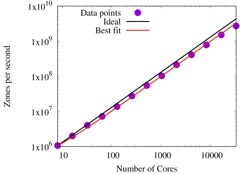
Figure 1: shows the weak scalability study of our 3D code. Each core processes 32x40x32 = 40960 number of zones. Scalability study has been performed on 8 to 32000 cores.

Figure 1 shows the weak scalability study (doubling of number of zones with doubling of cores) of the 3D version of this code on KISTI super-computer located at KAIST campus, Daejeon, South Korea. Scalability study has been performed on up to 32000 Intel KNL cores. We use a patch size of 32x40x32 zones per core for this weak scalability study. No saturation is observed up to 32000 cores.

4 Code Validation

In the following, we define $L_{1}$ error for a variable $Q$ as follows (Mignone, 2014):

$$L_{1}(Q)=\frac{\Sigma_{i}|\langle Q\rangle_{i}-\langle Q\rangle_{i}^{\rm ref}|\delta V_{i}}{\Sigma_{i}\delta V_{i}},$$

where, the summation over $i$ extends over all the grid zones, $\langle Q\rangle_{i}^{\rm ref}$ is volume average of reference solution and $\delta V_{i}$ is the zone volume.

4.1 One dimensional test problems

In this subsection, we present results of a couple of 1D test problems to demonstrate the convergence and correctness of our implementation for the second order algorithms.

4.1.1 Equilibrium cylindrical column

This one-dimensional test problem is designed to test the balance between the gradient of flux terms and the geometric source terms (gravitational potential set to zero) that arise in cylindrical coordinates. Such manufactured equilibrium configurations are constructed, e.g., in Mignone (2014); Ivan et al. (2015); Balsara et al. (2020) to demonstrate the accuracy convergence of the designed schemes. We solve the following conservation laws in one dimension:

$$\frac{\partial}{\partial t}\left[\begin{array}[]{ccccc}\rho\\ \rho v_{R}\\ \rho Rv_{\phi}\\ \rho v_{Z}\\ E\end{array}\right]+\frac{1}{R}\frac{\partial}{\partial R}\left[R\left(\begin{array}[]{ccccc}\rho v_{R}\\ \rho v_{R}^{2}+P\\ \rho Rv_{\phi}v_{R}\\ \rho v_{R}v_{Z}\\ \left(E+P\right)v_{R}\end{array}\right)\right]=\left[]\begin{array}[]{ccccc}0\\ \frac{\rho v_{\phi}^{2}}{R}+\frac{P}{R}\\ 0\\ 0\\ 0\end{array}\right]$$ (9)

As an initial condition, we choose an equilibrium rotating column with constant specific angular momentum $Rv_{\phi}=1$ and constant density $\rho=1$. The $R$ and $Z$ components of the velocity are also assumed to be zero: $v_{R}=v_{Z}=0$. Equilibrium pressure $P$ is chosen such that the gradient of radial flux term $\frac{1}{R}\frac{\partial}{\partial R}R\left(\rho v_{R}^{2}+P\right)$ exactly balances the source term $\frac{\rho v_{\phi}^{2}+P}{R}$. Solving this equality, we find equilibrium solution for pressure as $P(R)=P_{\rm in}+\frac{\rho Rv_{\phi}}{2}\left(\frac{1}{R_{\rm in}^{2}}-\frac{1}{R^{2}}\right)$. Here, $P_{\rm in}$ is the pressure at inner radius $R_{\rm in}$. Figure 2(a) shows the radial variation of $P(R)$ and $v_{\phi}(R)$ inside the column at the initial time ($t=0$).

This one-dimensional test problem has been run on a computational domain with radial extent [1:10] with 128 to 4096 uniformly divided zones. Equation 9 is evolved till a time of $t=10$. $P_{\rm in}=1$ and $\gamma=5/3$ are assumed. Initial analytical values are maintained in the ghost zones on both the inner and the outer radial boundaries (fixed boundary condition, Mignone, 2014; Balsara et al., 2018, 2020). Source term is calculated at the centroid of the mesh.

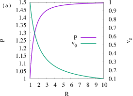
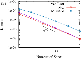
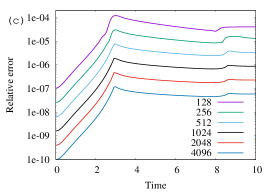
Figure 2: (a) shows the radial variation of P and $v_{\phi}$ while (b) shows the $L_{1}$ error convergence result in P for equilibrium cylindrical column test problem. All three reconstruction schemes, namely, MinMod, MC and van Leer show second order convergence. MC and van Leer are found to perform equally well in terms of $L_{1}$ error and better than MinMod. (c) shows the time variation of relative error for all the different mesh resolution with van Leer reconstruction. See text for details.

Figure 2(b) shows the convergence result of $L_{1}$ error in $P$ for Min-Mod, MC and Van Leer limiters. All the three schemes achieve the desired second order accuracy. Min-Mod converges slowly compared to the other two schemes. Figure 2(c) shows the time variation of the relative error of $P$ at $R=5$, which is defined as $(P(R=5,t)-P(R=5,t=0))/P(R=5,t=0)$, for different mesh resolution. This Figure is drawn for the runs where van Leer limiter is used for reconstruction. This result demonstrates that errors are converged by the end time of the simulation.

4.1.2 Standing shock solution in sub-Keplerian accretion

In this test problem, we compare the analytical and numerical shock solutions of sub-Keplerian accretion flow onto non-rotating black holes. We repeat the test problem presented in Fig. 1 of Molteni et al. (1996b). Numerical solution is performed in one-dimension (radial direction) on a computational domain of uniformly divided 256 zones in radial extent [0:50]. Simulations are run till a stopping time of $t=5000$. Matter enters the computational domain at $R=50$ with $V=\left(1.0,-0.08361221,0.036,0,0.010590145\right)$. We maintain these values in the outer radial boundary ghost zones. This $V$ corresponds to a specific energy $\epsilon=0.036$ and a specific angular momentum $l=1.8$ at $R=50$. These parameters are chosen from the parameter space corresponding to model H of Chakrabarti & Das (2001). To bring in the shock in the one-dimensional simulation, a perturbation at the outer boundary is required as explained in Chakrabarti & Molteni (1993). Here, we apply the perturbation in the form of increasing the pressure momentarily at the outer boundary ghost zones by a factor of 4 between time $t=1000$ and $t=1010$. We use pseudo-Newtonian potential (Paczyńsky & Wiita, 1980) to mimic the gravitational field around the non-rotating black hole. At the inner radial boundary, absorbing boundary condition is used to mimic the sucking of matter by the back hole. Thus, we set density and pressure to floor values $\rho_{\rm floor}=10^{-6}$, $P_{\rm floor}=10^{-8}$ and the velocity components to zero at all the zones inside the absorbing boundary region. Following Molteni et al. (1996b), we apply this absorbing conditions inside $R=1.5$.

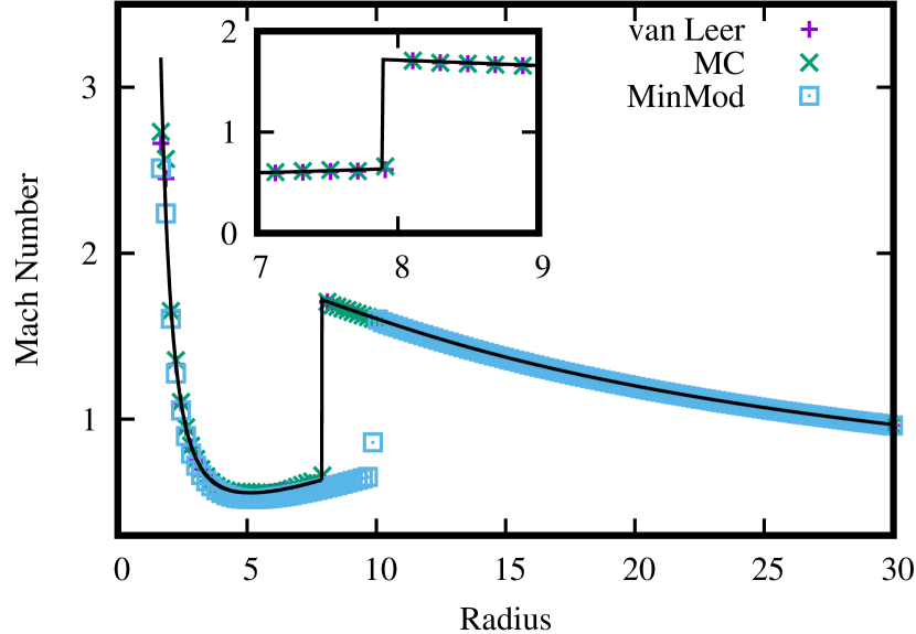
Figure 3: shows the radial variation of Mach number for standing shock solution in sub-Keplerian accretion test problem. Solid black line shows the analytical solution, whereas, the points show the numerical solutions for different reconstruction schemes. The zoomed part around the shock location i.e., around 7.89, is shown in the inlet. Both MC and van Leer are found to capture the shock exactly at the analytically predicted location.

The radial variation of Mach number ($M=v_{R}/a_{s}$) is shown in Figure 3. The radial range [0:30] is displayed here. The inner plot shows the zoomed in region around the shock location. Solid line shows the analytical solution and the different point styles show the zone-averaged numerical solutions at each grid for different schemes. According to theoretical calculations, the outer sonic point, shock location and inner sonic point are located at 27.9, 7.89 and 2.563, respectively. As can be seen, MC and van Leer capture all these points very well and follow the analytical solution mostly (except very close to inner boundary where curvature is very high). At this resolution (256 uniform zones), however, MinMod fails to follow the analytical solution starting from the shock location to the inner boundary. We have checked that at higher resolution, the matching for MinMod becomes better and at 1024 uniform zones or beyond the matching is acceptable (i.e., convergence of MinMod is slower).

4.2 Two dimensional test problems

In this subsection, we present results of another couple of 2D test problems to demonstrate the convergence and correctness of our implementation in multi-dimension.

4.2.1 Rotating thick torus

In this test problem, we numerically study the equilibrium configuration of the Newtonian thick torus. For this test problem, we assume Newtonian potential $\Phi(R,Z)=-1/\sqrt{R^{2}+Z^{2}}$. The equilibrium solution can be found analytically by removing the time-dependence $\frac{\partial}{\partial t}$ terms. We further assume axi-symmetry and remove $\frac{\partial}{\partial\phi}$ term also. The torus is supported by the balance between the inward gravitational pull and the combined outward push of pressure gradient and centrifugal force (Chakrabarti, 1996):

$$\frac{1}{\rho}\nabla P=-\nabla\Phi+\frac{l^{2}}{R^{3}}\nabla R,$$ (10)

where, $l=Rv_{\phi}$ is the angular momentum.For equation of state $P=K\rho^{\gamma}$ with $K$ as a constant measuring entropy and $l(R)=l_{0}$, a constant, we can solve Equation 10 to find

$$h\left(R,Z\right)+\Phi(R,Z)+\frac{l_{0}^{2}}{2R^{2}}=C,$$ (11)

where, $h$ is fluid specific enthalpy defined as $h=\frac{\gamma}{\gamma-1}\frac{P}{\rho}$ with $\gamma=4.0/3.0$ and $C$ is an integration constant. For our case, we assume $C=-0.06$ which gives us initially a torus as shown in Figure 4(a). Colors show the density. The density maximum for this torus is located at $(R,Z)=(4,0)$. The torus is embedded in a static background matter of constant density $\rho_{\rm floor}=10^{-8}$ and pressure $P_{\rm floor}=10^{-10}$. The background matter is free to evolve, but the density and pressure are floored according to the initial state (Porth et al., 2017).

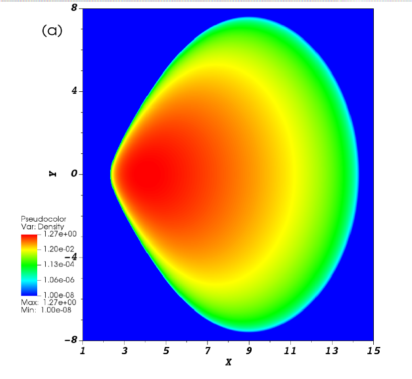
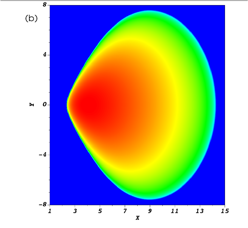
Figure 4: shows the initial (a) and final (b) density distribution for rotating thick torus. A mesh size of 1024x1024 and van Leer reconstruction are used for this simulation.

The simulations are run on a computation domain [1:20]$\times$[-10:10] with $128\times 128$ to $2048\times 2048$ uniform zones. For initialization of zone averaged quantities, we use 5-point Gaussian quadrature. All three types of reconstructions, namely, MinMod, MC and van Leer have been tried. Source terms are evaluated at centroid of the zones for this test problem. The simulations are run till a stopping time of $t=50$ which corresponds to nearly one full rotation period at the density maximum. Figure 4(b) shows the density of the torus at the final time.

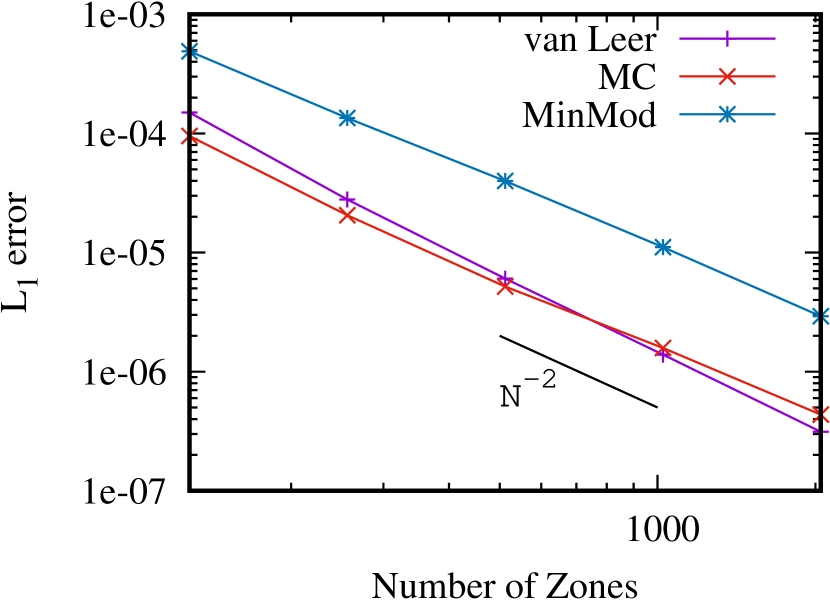
Figure 5: shows the L1 error convergence result in density for rotating thick torus test problem. All three reconstruction schemes, namely, MinMod, MC and van Leer show second order convergence. MC and van Leer are found to perform equally well in terms of $L_{1}$ error and better than MinMod.

Figure 5 shows the convergence result for all the three reconstruction procedures. $L_{1}$ errors are shown for density variable. All of them achieve desired second order accuracy. MinMod is found to have more dissipative solution. MC and van Leer performs equally well.

4.2.2 Bondi accretion in pseudo-Newtonian potential

In this test problem, we study the spherically symmetric, non-radiative Bondi accretion onto a non-rotating black hole. We use Paczynski-Wiita pseudo-Newtonian potential to mimic the gravitational field around the non-rotating black hole, which is defined as follows

$$\Phi\left(R,Z\right)=-\frac{1}{2\left(\sqrt{R^{2}+Z^{2}}-1\right)}.$$ (12)

The simulation is run in one quadrant of the $R-Z$ plane on a domain of [0:50]$\times$[0:50] using a uniform mesh of 256$\times$256 zones. van Leer limiter is used for reconstruction. The source terms are evaluated at the centroid of each zone. Reflection boundary conditions are used on the axis (i.e., $R=0$) and the equatorial plane (i.e., $Z=0$). Additionally, absorbing boundary condition is applied inside $r=1.5$ where $r=\sqrt{R^{2}+Z^{2}}$. Density and pressure are set to respective floor values, and velocities are set to zero on all the zones whose centroids fall inside $r=1.5$ (Molteni et al., 1996b; Garain et al., 2012). At the centroid of the outer boundary ghost zones (both $R$ and $Z$ boundaries), primitive variables are computed following the analytical solution and maintained throughout the simulation. Analytical solution for Bondi accretion in pseudo-Newtonian potential has been done following Section 2.1 of Ghosh et al. (2010). Solving Equation 4 of this reference, we can compute radial velocity $u(r)=\sqrt{v_{R}^{2}+v_{Z}^{2}}$ and subsequently, the sound speed $a_{s}(r)$ at radius $r$. This solution requires only one parameter, namely, the specific energy $\epsilon$ of the flow. For the present case, we choose $\epsilon=0.015$. Density at $r=50$ is normalized to 1, i.e., $\rho(r=50)=1.0$. This normalization allows us to find the density $\rho(r)$ at the centroid of the ghost zones since the accretion rate $\dot{m}=4\pi\rho ur^{2}$ is assumed to be a constant. Next, assuming adiabatic equation of state and $a_{s}^{2}=\frac{\gamma P}{\rho}$, we can evaluate $P(r)$ at the ghost zone centroids. We assume $\gamma=\frac{4}{3}$ for this simulation. For spherically symmetric Bondi accretion, $v_{\phi}=0$.

Initially, the interior is filled with a very low density, static matter with density $\rho_{\rm floor}=10^{-6}$ and pressure $P_{\rm floor}=10^{-10}$. Within a dynamical time (i.e., time required for the matter at outer boundary to reach the inner boundary), this background matter is washed away and steady state is reached within a couple of dynamical time.

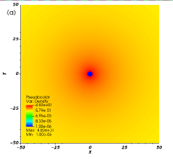
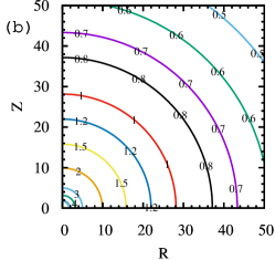
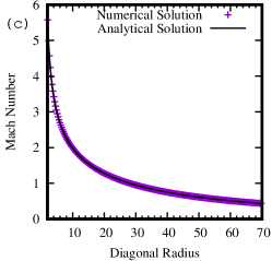
Figure 6: shows the results for Bondi accretion test problem at the final time $t=20000$. Left panel (a) shows the density distribution. Middle panel (b) shows the contour of constant Mach number ($u/a_{s}$). Both these results demonstrate that the code can retain spherical symmetry. On the right panel (c), we show comparative plot of the radial variation of Mach numbers along the diagonal direction. Solid line shows the analytical solution and the points show the numerical solution. A very good match is observed even at the inner radii where slope of the graph increases significantly.

Figure 6(a) shows steady state density map on log scale at a final time $t=20000$. This Figure has been drawn on $-50\leq R\leq 50$, $-50\leq Z\leq 50$ domain using reflection symmetry, although the computation has been performed only on the first quadrant. Figure 6(b) shows the labeled contours of constant Mach numbers. The contours are plotted between 0.5 at the outer part to 4 at the inner part. The circular nature of the contours is well maintained, even close to the axis and close to the absorbing boundary. Figure 6(c) shows the comparison of Mach numbers for the simulated flow and the analytical solution. For the numerical result, Mach number variation along the diagonal direction is drawn. Excellent matching between the two solutions can be observed.

5 3D Simulations

In this section, we present the results of the three dimensional simulations of the geometrically thick, sub-Keplerian, advective accretion flow onto a non-rotating black hole. We use van Leer limiter for all the simulations. The source terms are evaluated at the centroid of the zones. Paczynski-Wiita pseudo-Newtonian potential, as in the Bondi accretion test problem, is used to mimic the gravity for these cases as well.

We present results for a total of six simulations. Out of these, four simulations are done with axisymmetric inflow boundary condition at outer radial boundary and two simulations are done with non-axisymmetric perturbation applied. The details of the boundary conditions and the nature of perturbation is discussed in the following subsections. For a few simulations, we use ratioed mesh: $dx_{i+1}=\delta dx_{i}$, where, $dx_{i}$ represents the grid size of $i^{\rm th}$ zone in any direction and $\delta>1$ represents the common ratio.

5.1 Simulation set up and boundary conditions

Simulation set up:

Simulation parameters are documented in Table 1. Runs A1-A4 are done with axisymmetric inflow boundary condition and runs A5-A6 are extensions of run A3 with the inclusion of non-axisymmetric perturbation. Since the 3D simulations are very time consuming, we judiciously choose four set of flow parameters $\epsilon$ and $l$ (Col. 2 and 3 of Table 1) from different parts of the entire parameter space. As mentioned in Section 2, we focus on the parameter space corresponding to model V of Figure 2 in Chakrabarti & Das (2001). Flow parameters for run A1 have been picked up from the region just outside of the left boundary of the parameter space. Thus, analytically, this set of parameters does not produce a standing shock solution. Parameters for run A2, A3 and A4 have been picked up from the region just inside of the left boundary, mid-area and just inside of the right boundary of the parameter space, respectively. Analytically, standing shocks are expected at $R_{\rm sh}\sim 13,27$ and $48$ for runs A2, A3 and A4, respectively.

Column 4 of Table 1 shows the radial [0:R] and vertical domain [-Z:Z] of our simulation. In the azimuthal direction, domain is always [0:2$\pi$]. The choice of individual domain size for each run is to ensure that the shock surface remains well inside the domain for respective run. We also wish to study the dynamics of the turbulent post-shock region and therefore, choose the domain such that the post-shock region occupies a significant fraction of the entire computational domain and is well resolved. $R_{\rm sh}$ values provide an idea of the radial extent of the post-shock region, although prior multidimensional simulations showed that shock surface is located further out due to the presence of post-shock turbulence. Thus, we choose the radial domain size to be $\sim 4\times R_{\rm sh}$.

Column 5 shows the number of zones, N_R and N_Z, in $R$ and $Z$ directions, respectively. In $\phi$ direction, we always use 180 uniform zones. For runs A1 and A2, we use uniform zones in all directions. For run A3 (also A5 and A6), we use ratioed mesh in $R$ direction with common ratio of 1.003944 between successive radial zones. For run A4, we use ratioed mesh in both $R$ and $Z$ with common ratio 1.004235. In $Z$ direction, ratioing is done symmetrically about $Z=0$.

Boundary condition:

At upper and lower Z-boundaries, we use outflow boundary condition. Thus, we copy the primitive variables from the active zones to the adjacent ghost zones along these boundaries. Periodic boundary condition is enforced along the $\phi$ direction. On the axis (i.e., at $R=0$), reflective boundary condition is used: all the primitive variables except $v_{R}$ are symmetric across the axis (even function of $R$ near $R=0$) whereas $v_{R}$ takes minus sign across the axis (odd function of $R$ near $R=0$). To mimic the absorption of matter by black hole, an absorbing boundary, as discussed in 2D Bondi accretion problem, is placed inside $r=1.8$. Placement of this inner boundary at $r=1.8$ does not affect the dynamics of the post-shock flow much since the flow becomes supersonic between $r=$2 to 2.5.

Table 1: Parameters used for the simulations.

ID	$\epsilon$	$l$	Domain ($R$, $Z$)	NR, NZ	$t_{\rm stop}$	$u_{\rm r}$	$a_{s}$	Comments
A1	0.003	1.65	50, 50	320, 640	10000	0.07604	0.05706	uniform mesh; analytically no shock in accretion
A2	0.003	1.70	50, 50	320, 640	15000	0.07552	0.05708	uniform mesh; analytically shock at $\sim$ 13
A3	0.0022	1.75	100, 50	320, 640	20000	0.04822	0.04448	ratioed mesh in R with $\delta=1.003944$; analytically shock at $\sim$ 27
A4	0.0012	1.80	200, 100	440, 440	37000	0.03375	0.03216	ratioed mesh in R & Z (symmetric about Z=0) with $\delta=1.004235$; analytically shock at $\sim$ 48
A5	0.0022	1.75	100, 50	320, 640	27000	0.04822	0.04448	extended run A3 with non-axisymmetric density perturbation; momentarily 3% increase in mass accretion rate
A6	0.0022	1.75	100, 50	320, 640	27000	0.04822	0.04448	extended run A3 with non-axisymmetric density perturbation; momentarily 1.4% increase in mass accretion rate

At the upper radial boundary, we place inflow boundary condition. Matter enters the computational domain axi-symmetrically through all the zones with same radial velocity $u_{r}=\sqrt{v_{R}^{2}+v_{Z}^{2}}$ and sound speed $a_{s}$ (Molteni et al., 1996b). The density $\rho$ of the incoming matter is normalized to 1 at the outer boundary. Next, assuming adiabatic equation of state and $a_{s}^{2}=\frac{\gamma P}{\rho}$, we can evaluate pressure $P$ at the outer radial boundary. We assume $\gamma=\frac{4}{3}$ for all the simulations. Using the specific angular momentum values $l$, we can compute $v_{\phi}=l/R$ at the ghost zones.

The radial velocity $u_{r}$ and sound speed $a_{s}$ of the incoming matter are computed using the parameters $\epsilon$ and $l$. These $u_{r}$ and $a_{s}$ values are tabulated in Column 7 and 8, respectively. We maintain the primitive variables $V=\left(\rho=1.0,v_{R},v_{\phi},v_{Z},P\right)$ at all the ghost zones of the upper radial boundary throughout the simulation This implies a condition of constant accretion rate through outer radial boundary throughout the duration of our simulation.

Initial condition:

For simulations A1-A4, the interior is initially filled with a very low density, static background matter with density $\rho_{\rm floor}=10^{-6}$ and pressure $P_{\rm floor}=a_{s}^{2}\rho_{\rm floor}/\gamma$. Thus, the incoming matter initially rushes to the central black hole through nearly free space. Within a dynamical time or so, this background matter is washed away and a quasi-steady state is achieved soon after. These simulations are run till a stopping time of $t_{\rm stop}$, documented in column 5 of Table 1.

For runs A5 and A6, we take the final solution of run A3 as the initial condition. To apply perturbation, we follow similar simulation procedure as in Molteni et al. (1999), namely, perturb a (quasi-)steady state solution several units upstream of the shock and advect in the perturbation with the flow. We perturb the density in a small region at the upper radial boundary: ghost zone density is increased by a small factor for a small time duration and then maintained at the original value. We also maintain same boundary conditions as run A3 at upper and lower Z-boundaries and at the axis (i.e., $R=0$). Perturbation is applied for the time duration $21000\leq t\leq 21100$ and subsequently the simulations are run till a stopping time of $t_{\rm stop}=27000$.

5.2 Results with axisymmetric inflow boundary

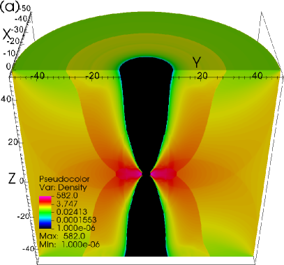
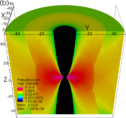
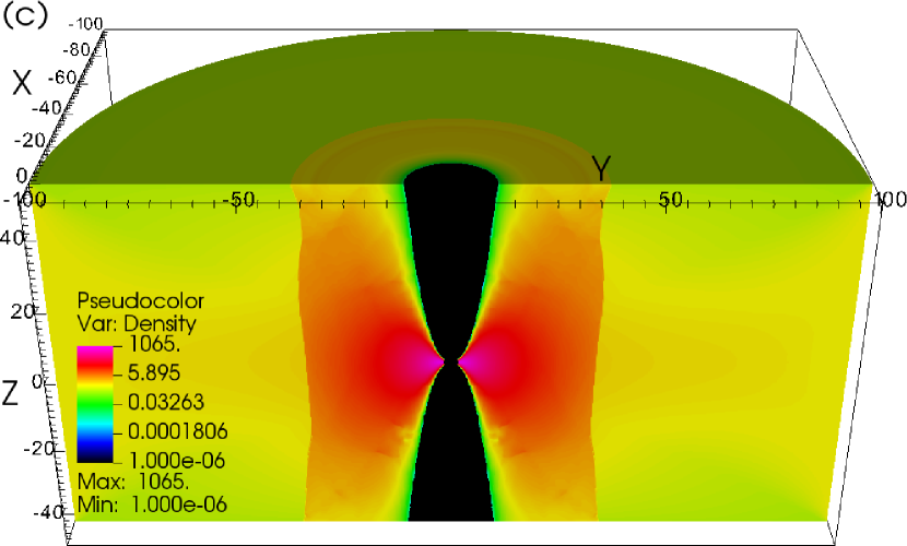
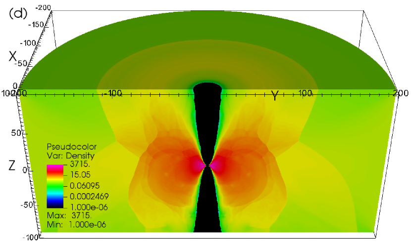
Figure 7: shows the density clips for all the cases A1-A4 (a: A1, b: A2, c: A3, d: A4) at the final time $t_{\rm stop}$ as listed in Table 1. Black color shows lower density and red color shows higher density.

Figure 7 shows the final state density clips for cases A1-A4. Normalized density values (normalized to 1 at outer radial boundary) on log scale are represented by color. Black color represents the floor density, whereas, the red color represents the higher density. For all the cases, a region surrounding the rotational axis (Z-axis) is devoid of matter primarily because of the non-zero angular momentum of the matter. On the other hand, higher density matter is found to be present in the region surrounding the equatorial area and close the central black hole. Flow density increases primarily for two reasons. Firstly, centrifugal barrier slows down nearly free-falling, sub-Keplerian incoming material as it approaches the central object. Because of this slow down, a density jump is observed (color becomes darker) somewhat away from the black hole. Secondly, because of the gravitational pull of the black hole, matter subsequently rushes towards the central part and hence, geometric compression further increases the density. The thermal pressure simultaneously increases, which puffs up the disk in the vertical direction. Thus, the denser matter forms the geometrically thick torus. Size of this torus depends on the the specific angular momentum value: higher the angular momentum, larger is the size of the torus. Outer boundary layer of this torus is named CENBOL.

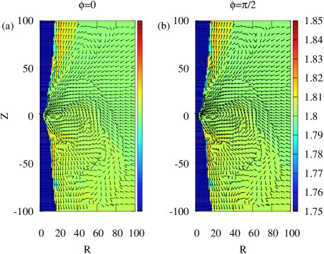
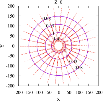
Figure 8: (a) and (b) show two slice plots of $l$ distribution, over-plotted with the $\left(v_{R},v_{Z}\right)$ vector field, at two different $\phi=$constant slices for run A4. Figures are drawn in radial range $0\leq R\leq 100$. As expected, $l$ remain mostly constant at the value 1.8 except slight redistribution in some part of post-shock regions. This is caused by the presence of post-shock turbulence which is demonstrated by the presence of in-plane vortices in the vector field. These two figures, drawn for two mutually perpendicular slices, are identical. (c) shows contours of constant $\log_{10}\rho$, over plotted with $(v_{R},v_{\phi})$ vector field, at $Z=0$ plane. Exact circular structure of the contours confirm the axisymmetry of density distribution. Additionally, the velocity vector field shows rotation dominated velocity field inside the post-shock region.

The torus remains axisymmetric for all the four runs A1-A4. Figure 7 shows symmetric density distribution in the right half (+ve Y-coordinates) and left half (-ve Y-coordinates). In fact, the axisymmetry can be investigated in any of the primitive fluid variables. Figure 8(a) and (b) show the $l$ distribution, over-plotted with velocity vector field $\left(v_{R},v_{Z}\right)$, at two mutually perpendicular $R-Z$ slices $\phi=0$ and $\phi=\pi/2$ at the final time for run A4. Length of an arrow is proportional to the logarithm of vector magnitude. Inner radial range $0\leq R\leq 100$ is shown here. $l(=1.8)$ is supposed to remain conserved, which we find almost everywhere except at most 3% change in the outflowing matter and some places in the post-shock region. This redistribution of $l$ is done by the turbulent eddies developed in the post-shock region. The vector field demonstrates the presence of such in-plane eddies. We compute zone-by-zone difference in the all the primitive variables for these two slices. For every zones and all variables, the result is zero showing that these two slices are identical. This confirms that the fluid configuration remains axisymmetric.

The axisymmetric distribution of density is also confirmed by the density contours on a $R-\phi$ slice ($Z=$constant plane). In Figure 8(c), we plot labeled density contours (logarithm base 10 of $\rho$) along with $\left(v_{R},v_{\phi}\right)$ velocity vectors at $Z=0$ plane. Density contours are perfectly circular both inside and outside the shock radius (contour marked 1.0). The vectors show rotational motion of the infalling material. Inside the shock radius, $v_{R}$ becomes very small and rotation dominates. However, as matter approaches towards the center, $v_{R}$ value starts increasing. For our simulation, angular momentum $l$ remains nearly conserved. Therefore, $v_{\phi}=l/R$ also increases along with $v_{R}$.

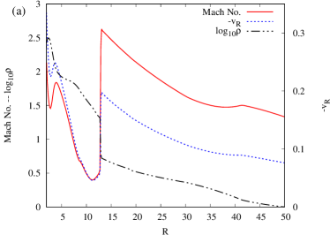
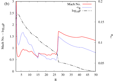
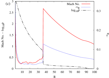
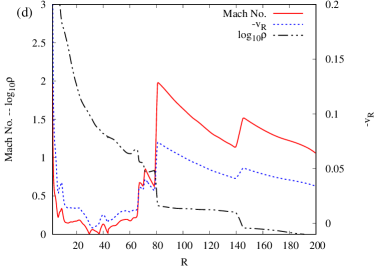
Figure 9: shows the radial variation of Mach number, ${\rm log_{10}}\rho$ (left y-axis) and negative values of $v_{R}$ (right y-axis) along the equator at the final time for runs A1-A4 (a: A1, b: A2, c: A3, d: A4).

At CENBOL, radial gradient of different quantities such as density, radial velocity, Mach number etc. changes abruptly. In Figure 9(a)-(d), we plot the radial variation of these quantities along the equator for runs A1-A4, respectively. On left y-axis, Mach number and log base 10 values of $\rho$ are shown. On right y-axis, negative values of $v_{R}$ values are shown. These plots are drawn, again, at the respective $t_{\rm stop}$ time. The shock location can be identified by the abrupt super-sonic ($M>1$) to sub-sonic ($M<1$) transition point as one moves inward from the outer radial boundary. Flow again makes another sub-sonic to super-sonic transition closer to the black hole before disappearing through the inner radial boundary. However, this transition is smooth. At the shock location, $\rho$ value increases by a factor of 2–4 (as found in these plots) because of the equivalent decrease in $v_{R}$ value to maintain mass conservation. Corresponding reduction in kinetic energy is converted into thermal energy and the flow temperature increases. Thus, the immediate post-shock region becomes hotter and denser. With reducing $R$ values, $\rho$ further increases by order of magnitude, primarily because of geometric compression.

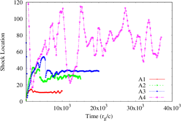
Figure 10: shows the time variation of the shock location at the equator for cases A1-A4. All the simulations are run till a quasi-steady state is achieved.

The shock location is found to be dynamic, which makes the entire post-shock torus dynamic as well. Figure 10 shows the time variation of the shock location for cases A1-A4. Size of the dynamical eddies that form inside the post-shock region determines the amplitude of variation. Figure 8(a) and (b) show examples of such in-plane eddies. For run A4, the variation in radial distance is found to be very large. Such oscillations of the post-shock torus are found in prior simulations and are believed to be the origin of low frequency quasi-periodic oscillations seen in many black hole X-ray binaries (Molteni et al., 1996a; Chakrabarti et al., 2004; Garain et al., 2014; Suková & Janiuk, 2015; Suková et al., 2017). As can be seen in this Figure, all the runs reached a quasi-steady state by the simulation end time. Also, it is evident that the average shock location is at larger radial distance than the analytically predicted location (see last column of Table 1). This was already understood in earlier multi-dimensional simulations that turbulent pressure additionally push the shock surface radially outward.

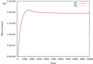
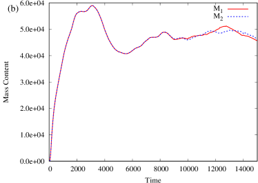
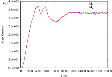
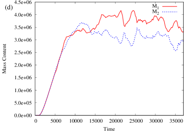
Figure 11: shows the time variation of total masses M₁ and M₂ in two halves, above and below the equator respectively, for cases A1-A4 (a: A1, b: A2, c: A3, d: A4). For higher angular momenta runs (i.e., for A3 and A4), we see that the plots for M₁ and M₂ are 180^∘ out of phase. This implies a vertical oscillation of the disk matter about the equator.

Because of the turbulence, the torus develops asymmetry about the equatorial plane, as found earlier (Chakrabarti et al., 2004; Deb et al., 2016; Suková et al., 2017). This asymmetry in density becomes prominent for the run A4 from Figure 7(d). In order to quantify the density asymmetry about the equatorial plane, we compute the total mass above ($M_{1}$) and below ($M_{2}$) the equator at any time $t$. We define these two quantities as follows:

$$M_{1}(t)=\int_{0}^{Z_{\rm out}}\int_{0}^{2\pi}\int_{0}^{R_{\rm out}/2}\rho(t)RdRd\phi dZ,$$

$$M_{2}(t)=\int_{-Z_{\rm out}}^{0}\int_{0}^{2\pi}\int_{0}^{R_{\rm out}/2}\rho(t)RdRd\phi dZ,$$

where, $R_{\rm out}$ and $Z_{\rm out}$ represent respectively the radial and vertical endpoints of the computational domain. Since $\rho$ is higher in the region surrounding the equator and close to the black hole, major contribution in the above integrals comes from this part. Figure 11 shows the time variations of $M_{1}$ and $M_{2}$ for runs A1-A4. For runs A1 and A2 (i.e., Figure 11(a) and (b)), we don’t observe any significant asymmetry throughout the simulation. However, we observe the difference in $M_{1}$ and $M_{2}$ for runs A3 and A4 (i.e., Figure 11(c) and (d)) after the runs reach a quasi-steady state. Interestingly, the two plots are 180^∘ out of phase, i.e., when mass increases in one half, same amount decreases in other half. This implies a vertical oscillation of the disk matter about the equator.

5.3 Flow with density perturbation

In this sub-section, we present results of the simulations with non-axisymmetric azimuthal perturbation. Two simulations are conducted with different magnitude of perturbations. For run A5, we increase the ghost zone density momentarily by a factor of 1.2 in a small region of azimuthal width $\Delta\phi=\pi/10$ centered around $\phi=\pi/4$ and vertical width $\Delta Z=50$ centered about equatorial plane. This density perturbation corresponds to a momentarily 3$\%$ increase in the mass accretion rate through the outer radial boundary. For run A6, we increase the ghost zone density momentarily by a factor of 1.1 in a small region of azimuthal width $\Delta\phi=\pi/10$ centered around $\phi=\pi/4$ and vertical width $\Delta Z=25$ centered about equatorial plane. This density perturbation corresponds to a momentarily 1.4$\%$ increase in the mass accretion rate through the outer radial boundary.

Both the simulations show that the axisymmetric shape of the shock surface is deformed, possibly due to the the occurrence of standing accretion shock instability (SASI). The actual mechanism for SASI is not yet fully understood. Foglizzo & Tagger (2000) argue that an entropic-acoustic cycle in the post-shock region triggers the instability. In this model, an inward propagating entropy perturbation (which is caused by the increased density in our simulation) triggers an outward propagating acoustic wave. After reaching the shock surface, this acoustic wave triggers new inward propagating entropy wave and the cycle continues. Successive outward propagating acoustic waves lead to the instability of the shock surface. On the other hand, Blondin & Mezzacappa (2006) argued that purely acoustic waves originating from the density (or pressure) inhomogeneities can produce SASI.

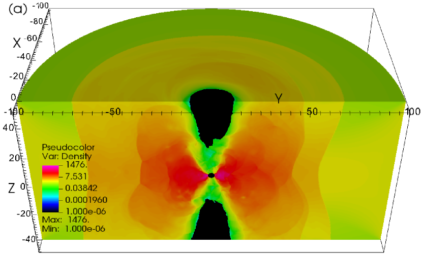
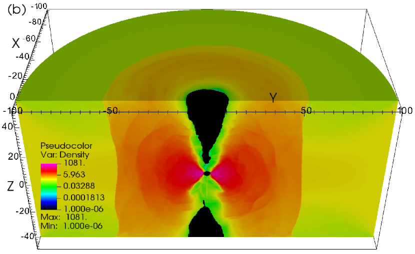
Figure 12: shows the density clips for (a) A5 and (b) A6 at the final time $t_{\rm stop}=27000$. Black color shows lower density and red color shows higher density.

Figure 12 shows the final state density clips for runs A5 (a) and A6 (b) at time $t_{\rm stop}=27000$. These clips can be compared with the non-perturbed counterpart in Figure 7c. Clearly, a deformation in the shape of the outer boundary of the density torus is identifiable. For these Figures, the shock surface coincides with the outer boundary of the density torus. The outer boundary also moved radially outward. More deformation is seen in the case of A5 compared to A6 because the initial perturbation strength is higher for A5. The axisymmetric structure of density distribution is also seen to be broken. Density distribution in the right half (+ve Y-coordinates) and left half (-ve Y-coordinates) is clearly different. We also notice that some region above and below the black hole and surrounding the rotational axis is occupied by low density matter. This is mostly low angular momentum, infalling matter as explained in the next paragraph. However, the presence of this matter causes the simulation time-steps $dt$ to reduce by two orders of magnitude since the length scale $rd\phi$ close to the axis is very small and Courant condition picks up $dt$ from this region.

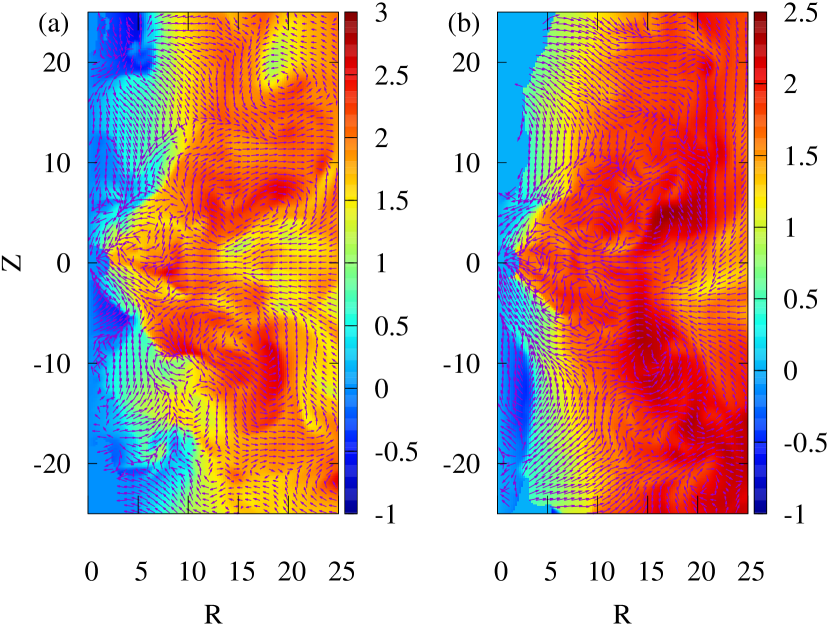
Figure 13: shows the slice plots of $l$ distribution, overplotted with $(v_{R},v_{Z})$ vector field, at $\phi=0$ slice in the inner part 0$\leq R\leq$ 25 and -25$\leq Z\leq$25 of the simulation domain for (a) A5 and (b) A6 at the final time $t_{\rm stop}=27000$. At the outer boundary, $l=1.75$ for these runs. However, we observe significant redistribution of $l$ in the inner part.

Flow is found to be more turbulent in comparison to it’s non-perturbed counterpart in Figure 7(c). This turbulence results significant amount of angular momentum re-distribution inside the post-shock region. We plot the specific angular momentum ($l$) distribution on $\phi=0$ slice in the range $0\leq R\leq 25$ and $-25\leq Z\leq 25$. Colors in Figure 13(a) and (b) show the $l$ distribution for cases A5 and A6, respectively. We also overplotted the $\left(v_{R},v_{Z}\right)$ vector field in these plots. Length of an arrow is proportional to the logarithm of vector magnitude. The vector field demonstrates the presence of in-plane turbulent eddies.

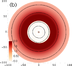
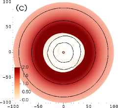
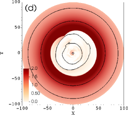
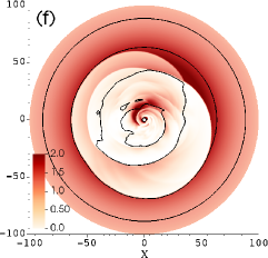
Figure 14: shows Mach number color maps over plotted with density contours at the equatorial plane at successive times: (a) 22000, (b) 23000, (c) 24000, (d) 25000, (e) 26000 and (f) 27000 for run A5. Contours are drawn for $\rho$ values 1.1 (outermost), 1.3, 8 and 30 (innermost) Towards the end of the simulation, we find that, in addition to the outer shock (super-sonic to sub-sonic transition), flow develops internal shock as well.

Figure 14 shows the Mach number color maps overplotted with labelled density contours for run A5 at the equatorial plane at successive times: (a) at time 22000, (b) at 23000, (c) at 24000, (d) at 25000, (e) at 26000 and (f) at 27000. The shock is clearly indentifiable from the color contrast. Initial density perturbation, introduced at $t=21000$ at the outer radial radial boundary, reaches the shock surface at around $t=22000$ (see the deformation of density contour in the post-shock region in (a)). As the perturbation enters the sub-sonic region, the shock front gets slightly distorted and very small amplitude oscillations sets in. In the post-shock region, rotational motion is dominated over radial motion. Therefore, the perturbation gets elongated as it further advects towards the black hole. At the same time, geometrical compression of the dense gas produce acoustic waves which travel upstream towards the shock front and add up to the existing small amplitude oscillations. However, we do not observe any significant distortion of shock front during it’s radial movement upto the inner sonic point at $R\sim 2$ (see Figure 14(b)). After this point, between time $t=$23000 and 24000 (i.e., between Figure 14(b) and (c)), significant acoustic feedback originating from the interior regions travels upstream and reach the shock front. Our modal analysis (see below) confirms the presence of different oscillation modes of nearly equal amplitude around this time. Because of the non-linear mode mixing during this time, the distortion of the shock surface starts growing (see Figure 14(c)). With increasing time, the instability further grows.

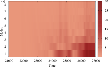
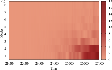
Figure 15: shows the time variation (X-axis) of amplitudes (colors) for different modes $m$ (Y-axis) for run (a) A5 and (b) A6. We see dominance of $m=$1 and 2 towards the end of our simulations.

We also perform the modal analysis of this equatorial shock front oscillation. Following Nagakura & Yamada (2008), we utilize following formula to calculate the Fourier amplitude $a_{m}(t)$ corresponding to mode $m$ at time $t$:

$$a_{m}(t)=\int_{0}^{2\pi}R_{\rm sh}(\phi,t)e^{im\phi}d\phi$$ (13)

Colors in Figure 15 show the amplitude $|a_{m}|$ as a function of time (X-axis) for modes 1–8 (Y-axis). Panel (a) represents the modal analysis for run A5 and panel (b) represents the same for run A6. With increasing time, we find the increasing amplitude in various modes. Towards the end of the simulations, we find the dominance of $m=$1 and 2 modes. This is consistent with the findings of Yamasaki & Foglizzo (2008) who also found dominance of $m=$1 and 2 modes in SASI for cylindrical accretion shock structure in the context of core-collapse supernova.

6 Summary and Concluding Remarks

In this work, we investigate the dynamics of the sub-Keplerian matter accretion onto a non-rotating black hole using three dimensional inviscid hydrodynamics. Specifically, we aim to study through numerical simulations whether the centrifugal pressure shock surface remains stable or not when all three dimensions are dynamically active. Majority of the previous numerical simulations of such accreition disk are done with axisymmetric or thin disk assumptions and are conducted with at most two dynamically active dimensions. We also want to see whether the turbulence, present inside the post-shock region, induce any non-axisymmetric perturbation to the shock surface. Prior analyses reported that such perturbation might lead to standing accretion shock instability (SASI) inside the accretion disk.

For the above mentioned investigation, we develop an inviscid Euler equations solver in cylindrical coordinates following the numerical algorithms given in Mignone (2014). To validate the correct implementation and performance of our code, we perform convergence tests using known equilibrium solutions. We also test the shock capturing capability by reproducing the analytic solution of standing shock formation in sub-Keplerian matter accretion onto a non-rotating black hole.

Having performed the benchmark test problems, we apply our code for the 3D simulation of sub-Keplerian matter accretion. Below we list our main findings:

• The sub-Keplerian accreting matter is found to self-consistently form the centrifugal barrier supported shock surface. Inside the post-shock region, matter velocity is primarily rotation dominated resembling a property of geometrically thick disks. However, as the matter moves more towards the black hole, the magnitude of radial velocity increases.

• The dynamical vortices seem to form as it is seen in axisymmetric two-dimensional simulation. However, relaxing the axisymmetric assumption does not introduce any non-axisymmetry or instability inside the thick disk.

• Vertical oscillations of the disk matter is found as is reported earlier in Chakrabarti et al. (2004); Deb et al. (2016); Suková et al. (2017).

• By introducing explicit non-axisymmetric density perturbation, we find that SASI is developed inside the accretion disk.

Radiative process such as inverse-Compton cooling of electrons inside the post-shock matter can produce inhomogeneous temperature and pressure distribution. This can induce non-axisymmetric perturbation to the shock surface and produce SASI. Coupling the 3D hydro simulation with a Monte Carlo based radiative transfer code (Garain et al., 2012, 2014) could provide us an opportunity to investigate the occurrence of SASI inside the sub-Keplerian flow in presence of radiative cooling. We wish to take up such work in future.

Data Availability

Numerically simulated data are available on reasonable request from the corresponding author.

References

- Balsara (2017) Balsara D. S., 2017, Living Reviews in Computational Astrophysics, 3, 2
- Balsara et al. (2018) Balsara D. S., Garain S., Taflove A., Montecinos G., 2018, Journal of Computational Physics, 354, 613
- Balsara et al. (2020) Balsara D. S., Garain S., Florinski V., Boscheri W., 2020, Journal of Computational Physics, 404, 109062
- Blondin & Mezzacappa (2006) Blondin J. M., Mezzacappa A., 2006, ApJ, 642, 401
- Chakrabarti (1989a) Chakrabarti S. K., 1989a, ApJ, 337, L89
- Chakrabarti (1989b) Chakrabarti S. K., 1989b, ApJ, 347, 365
- Chakrabarti (1990) Chakrabarti S. K., 1990, Theory of Transonic Astrophysical Flows, doi:10.1142/1091.
- Chakrabarti (1996) Chakrabarti S. K., 1996, Phys. Rep., 266, 229
- Chakrabarti & Das (2001) Chakrabarti S. K., Das S., 2001, MNRAS, 327, 808
- Chakrabarti & Manickam (2000) Chakrabarti S. K., Manickam S. G., 2000, ApJ, 531, L41
- Chakrabarti & Molteni (1993) Chakrabarti S. K., Molteni D., 1993, ApJ, 417, 671
- Chakrabarti & Molteni (1995) Chakrabarti S. K., Molteni D., 1995, MNRAS, 272, 80
- Chakrabarti & Titarchuk (1995) Chakrabarti S., Titarchuk L. G., 1995, ApJ, 455, 623
- Chakrabarti et al. (2004) Chakrabarti S. K., Acharyya K., Molteni D., 2004, A&A, 421, 1
- Chang & Ostriker (1985) Chang K. M., Ostriker J. P., 1985, ApJ, 288, 428
- Cui et al. (1997) Cui W., Zhang S. N., Focke W., Swank J. H., 1997, ApJ, 484, 383
- Deb et al. (2016) Deb A., Giri K., Chakrabarti S. K., 2016, MNRAS, 462, 3502
- Deb et al. (2017) Deb A., Giri K., Chakrabarti S. K., 2017, MNRAS, 472, 1259
- Falle (1991) Falle S. A. E. G., 1991, MNRAS, 250, 581
- Foglizzo & Tagger (2000) Foglizzo T., Tagger M., 2000, A&A, 363, 174
- Fukue (1987) Fukue J., 1987, PASJ, 39, 309
- Garain et al. (2012) Garain S. K., Ghosh H., Chakrabarti S. K., 2012, ApJ, 758, 114
- Garain et al. (2014) Garain S. K., Ghosh H., Chakrabarti S. K., 2014, MNRAS, 437, 1329
- Garain et al. (2015) Garain S., Balsara D. S., Reid J., 2015, Journal of Computational Physics, 297, 237
- Garain et al. (2020) Garain S. K., Balsara D. S., Chakrabarti S. K., Kim J., 2020, ApJ, 888, 59
- Ghosh et al. (2010) Ghosh H., Garain S. K., Chakrabarti S. K., Laurent P., 2010, International Journal of Modern Physics D, 19, 607
- Giri & Chakrabarti (2013) Giri K., Chakrabarti S. K., 2013, MNRAS, 430, 2836
- Giri et al. (2015) Giri K., Garain S. K., Chakrabarti S. K., 2015, MNRAS, 448, 3221
- Gropp et al. (1999) Gropp W., Lusk E., Skjellum A., 1999, Using MPI: Portable Programming with the Message-Passing Interface. MIT press
- Hawley et al. (1984) Hawley J. F., Smarr L. L., Wilson J. R., 1984, ApJS, 55, 211
- Ivan et al. (2015) Ivan L., De Sterck H., Susanto A., Groth C. P. T., 2015, Journal of Computational Physics, 282, 157
- Janiuk et al. (2008) Janiuk A., Proga D., Kurosawa R., 2008, ApJ, 681, 58
- Janiuk et al. (2009) Janiuk A., Sznajder M., Mościbrodzka M., Proga D., 2009, ApJ, 705, 1503
- Kim et al. (2017) Kim J., Garain S. K., Balsara D. S., Chakrabarti S. K., 2017, MNRAS, 472, 542
- Kim et al. (2019) Kim J., Garain S. K., Chakrabarti S. K., Balsara D. S., 2019, MNRAS, 482, 3636
- Kurosawa & Proga (2009) Kurosawa R., Proga D., 2009, ApJ, 693, 1929
- Lanzafame et al. (1998) Lanzafame G., Molteni D., Chakrabarti S. K., 1998, MNRAS, 299, 799
- Lanzafame et al. (2008) Lanzafame G., Cassaro P., Schilliró F., Costa V., Belvedere G., Zappalá R. A., 2008, A&A, 482, 473
- LeVeque et al. (2002) LeVeque R., J L., Crighton D., 2002, Finite Volume Methods for Hyperbolic Problems. Cambridge Texts in Applied Mathematics, Cambridge University Press, https://books.google.co.in/books?id=QazcnD7GUoUC
- Lee et al. (2016) Lee S.-J., Chattopadhyay I., Kumar R., Hyung S., Ryu D., 2016, ApJ, 831, 33
- Mignone (2014) Mignone A., 2014, Journal of Computational Physics, 270, 784
- Molteni et al. (1994) Molteni D., Lanzafame G., Chakrabarti S. K., 1994, ApJ, 425, 161
- Molteni et al. (1996a) Molteni D., Sponholz H., Chakrabarti S. K., 1996a, ApJ, 457, 805
- Molteni et al. (1996b) Molteni D., Ryu D., Chakrabarti S. K., 1996b, ApJ, 470, 460
- Molteni et al. (1999) Molteni D., Tóth G., Kuznetsov O. A., 1999, ApJ, 516, 411
- Monchmeyer & Muller (1989) Monchmeyer R., Muller E., 1989, A&A, 217, 351
- Mondal & Chakrabarti (2021) Mondal S., Chakrabarti S. K., 2021, ApJ, 920, 41
- Nagakura & Yamada (2008) Nagakura H., Yamada S., 2008, ApJ, 689, 391
- Nagakura & Yamada (2009) Nagakura H., Yamada S., 2009, ApJ, 696, 2026
- Okuda et al. (2007) Okuda T., Teresi V., Molteni D., 2007, MNRAS, 377, 1431
- Okuda et al. (2019) Okuda T., Singh C. B., Das S., Aktar R., Nandi A., Dal Pino E. M. d. G., 2019, PASJ, 71, 49
- Paczyńsky & Wiita (1980) Paczyńsky B., Wiita P. J., 1980, A&A, 500, 203
- Patra et al. (2019) Patra D., Chatterjee A., Dutta B. G., Chakrabarti S. K., Nandi P., 2019, ApJ, 886, 137
- Porth et al. (2017) Porth O., Olivares H., Mizuno Y., Younsi Z., Rezzolla L., Moscibrodzka M., Falcke H., Kramer M., 2017, Computational Astrophysics and Cosmology, 4, 1
- Porth et al. (2019) Porth O., et al., 2019, ApJS, 243, 26
- Radhika et al. (2016) Radhika D., Nandi A., Agrawal V. K., Mandal S., 2016, MNRAS, 462, 1834
- Ryu et al. (1995) Ryu D., Brown G. L., Ostriker J. P., Loeb A., 1995, ApJ, 452, 364
- Ryu et al. (1997) Ryu D., Chakrabarti S. K., Molteni D., 1997, ApJ, 474, 378
- Shang et al. (2019) Shang J. R., Debnath D., Chatterjee D., Jana A., Chakrabarti S. K., Chang H. K., Yap Y. X., Chiu C. L., 2019, ApJ, 875, 4
- Singh et al. (2021) Singh C. B., Okuda T., Aktar R., 2021, Research in Astronomy and Astrophysics, 21, 134
- Suková & Janiuk (2015) Suková P., Janiuk A., 2015, MNRAS, 447, 1565
- Suková et al. (2017) Suková P., Charzyński S., Janiuk A., 2017, MNRAS, 472, 4327
- Toro (2009) Toro E., 2009, Riemann Solvers and Numerical Methods for Fluid Dynamics: A Practical Introduction. Springer Berlin Heidelberg, https://books.google.co.in/books?id=SqEjX0um8o0C
- Yamasaki & Foglizzo (2008) Yamasaki T., Foglizzo T., 2008, ApJ, 679, 607
- Ziegler (2011) Ziegler U., 2011, Journal of Computational Physics, 230, 1035