Joint SPX–VIX calibration with Gaussian polynomial volatility models: deep pricing with quantization hints

Abstract

We consider the joint SPX-VIX calibration within a general class of Gaussian polynomial volatility models in which the volatility of the SPX is assumed to be a polynomial function of a Gaussian Volterra process defined as a stochastic convolution between a kernel and a Brownian motion. By performing joint calibration to daily SPX-VIX implied volatility surface data between 2012 and 2022, we compare the empirical performance of different kernels and their associated Markovian and non-Markovian models, such as rough and non-rough path-dependent volatility models. In order to ensure an efficient calibration and a fair comparison between the models, we develop a generic unified method in our class of models for fast and accurate pricing of SPX and VIX derivatives based on functional quantization and Neural Networks. For the first time, we identify a conventional one-factor Markovian continuous stochastic volatility model that is able to achieve remarkable fits of the implied volatility surfaces of the SPX and VIX together with the term structure of VIX futures. What is even more remarkable is that our conventional one-factor Markovian continuous stochastic volatility model outperforms, in all market conditions, its rough and non-rough path-dependent counterparts with the same number of parameters.

JEL Classification:

G13, C63, G10.

Keywords:

SPX and VIX modeling, Stochastic volatility, Gaussian Volterra processes, Quantization, Neural Networks.

1 Introduction

Launched in 1993 by the CBOE, the VIX has become one of the most widely followed volatility index. It represents an estimation of the S&P 500 index (SPX) expected volatility over a one-month period. More precisely, the VIX is calculated by aggregating weighted prices of SPX puts and calls over a wide range of strikes and maturities [20]. By construction, the VIX expresses an interpolation between several points of the SPX implied volatility term structure. Thus, the task of modeling and pricing VIX options for a given maturity $T$ naturally requires some consistency with SPX options maturing up to one month ahead of $T$. Furthermore, computing the implied volatility of VIX options using Black’s formula requires VIX futures that also need to be priced consistently.

By joint SPX–VIX calibration problem, we mean the calibration of a model across several maturities to European call and put options on SPX and VIX together with VIX futures. Such joint calibration turns out to be quite challenging for several reasons: multitude of instruments to be calibrated (SPX and VIX call/put options, VIX futures) across several maturities (to stay consistent with the construction of the VIX), characterized by low levels of implied volatilities of the VIX with an upward slope, in contrast with the important at-the-money (ATM) SPX skew that becomes more pronounced for smaller maturities.

In recent years, substantial progress has been made in developing relatively sophisticated stochastic models that achieve decent joint fits by exploiting a wide variety of mathematical tools such as jump processes [8, 21, 43, 46, 52], rough volatility [16, 30, 56], path-dependent volatility [36] and multiple-factors [26, 32, 36, 55]. However, examples of illustrated fits of these models are usually partial: in some cases VIX futures are not calibrated; in other cases VIX derivatives are calibrated up to maturity slice $T$, while the SPX derivatives for maturity slices $T+\Delta$ for $\Delta\in(0,1\text{ month})$ are missing. Although different in their mathematical nature, these models share in common the fact that they allow for 1) large price movements of the SPX on very short time scales with some forms of spikes in the ‘instantaneous’ volatility process due to a large ‘vol-of-vol’, and 2) fast mean reversions towards relatively low volatility regimes. We believe these are the two crucial ingredients for the joint calibration problem.

The aforementioned literature generally agrees that conventional one-factor continuous Markovian stochastic volatility models are not able to achieve a decent joint calibration. Our main motivations can be stated as follows:

Can joint calibration be achieved without appealing to multiple-factors, jumps, roughness or path-dependency?

Is joint calibration possible with conventional one-factor continuous Markovian models?

In a nutshell, we show in this paper that the answer to both questions is a resounding: Yes. By performing joint calibration on daily SPX-VIX implied volatility surface data between 2012 and 2022 using a large class of models, we identify for the first time a conventional one-factor Markovian continuous stochastic volatility model that is able to achieve remarkable fits for a wide range of maturity slices $[T_{s},T_{e}]$ for VIX implied volatility surface and of maturity slices $[T_{s},T_{e}+1\text{ month}]$ for SPX implied volatility surface, together with the term structure of VIX futures as shown on Figure 1. What is even more remarkable is that our conventional one-factor Markovian continuous stochastic volatility model outperforms its rough and non-rough path-dependent counterparts with the same number of parameters: 6 effective parameters that govern the dynamics of the model in addition to the usual input curve that allows to match certain term structures.

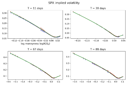
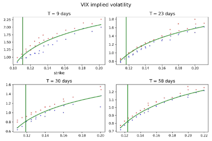
Figure 1: SPX–VIX smiles (bid/ask in blue/red) and VIX futures (vertical black lines) jointly calibrated with our conventional continuous stochastic volatility model (full green lines) produced by the exponential kernel $K^{exp}$, 23 October 2017.

More precisely, our methodology and contributions are summarized as follows:

Gaussian polynomial volatility models.

First, we introduce in Section 2 a general class of Gaussian polynomial volatility models in which the SPX spot price takes the form

$$\frac{dS_{t}}{S_{t}}=\sigma_{t}\left(\rho dW_{t}+\sqrt{1-\rho^{2}}dW_{t}^{\perp}\right),$$

where $(W,W^{\perp})$ is two-dimensional Brownian motion. The SPX spot price $S$ is correlated with the volatility process $\sigma$ which is, up to a normalizing constant, defined as a polynomial function $p(X)$ of a Gaussian Volterra process $X$ in the form

$$X_{t}=\int_{0}^{t}K(t-s)dW_{s},$$

for a locally square-integrable kernel $K$. The choice of the kernel introduces a good deal of flexibility in the modeling of the volatility process, such as rough volatility [2, 4, 5, 10, 13, 24, 29, 30] for singular fractional kernels of the form $K(t)\sim t^{H-1/2}$ with $0<H{\leq}1/2$, or the log-modulated kernel that extends the fractional kernel for the case $H=0$, see [12]; path-dependent models with non-singular kernel such as the shifted fractional kernel $K(t)\sim(t+\varepsilon)^{H-1/2}$; exponential kernels $K(t)\sim e^{-\lambda t}$ for which $X$ is a (Markovian) Ornstein-Uhlenbeck process or weighted sums of exponentials [1, 3, 22, 39], refer to Table 1 below. We will compare the performance of these different kernels on the joint calibration problem. Although it is difficult to decouple the impact of the different input parameters of the model, it turns out, that the choice of $K$ has a major impact on the ATM-skew of the implied volatility of the SPX and the level of the implied volatility of the VIX. While the choice of the polynomial function $p$ has a prominent impact on the shape of the VIX smile. Taking $p$ a polynomial of order $5$ (and higher) allows us to reproduce the upward slope of the VIX smile.

Generic, fast and accurate pricing via quantization and Neural Networks.

Second, in order to to ensure a fair comparison between the calibrated models with different kernels across 10 years of daily joint implied volatility surfaces, we develop a generic unified method that applies to any Gaussian polynomial volatility model for pricing SPX and VIX derivatives in an efficient and accurate fashion. The method is based on functional quantization and Neural Networks. The tractability of the quantization approach highly relies on the Gaussian nature of $X$ combined with the polynomial form of the volatility process $\sigma$. More precisely:

• Fast pricing of VIX derivatives via Quantization: we develop in Section 4 a functional quantization approach for computing VIX derivatives in our class of Gaussian polynomial volatility models.

  When computing expectations in the form of $\mathbb{E}[F(Y)]$ where no closed form solution is available, a fast alternative to Monte Carlo is quantization. The idea is to approximate the random variable $Y$ with a discrete random variable $\widehat{Y}$ to compute efficiently the (conditional) expectations of suitable functionals of $Y$. Quantization was first developed in the 1950’s for signal processing [31, 33] and more recently has been studied for applications in numerical probability [48] and mathematical finance [49, 53]. We will exploit the Gaussian nature of the process $X$ to develop a functional quantization approach.

  A first attempt to use functional quantization for VIX futures in the context of the rough Bergomi model appears in [17]. Unfortunately, the method is not precise enough in practice, especially for the fractional kernel with small values of $H$ even with a lot of quantization trajectories, see [17, Figure 3] where the number of quantized points were pushed as far as $N=1,000,000$ but the approximated values for VIX futures are still well-off the correct values, see also Figure 6 below. It is well known that the convergence of the quantization for fractional processes is very slow of order $1/(\log N)^{H}$, see [23].

  Using a crucial moment-matching trick, see (4.17), we are able to make functional quantization usable in practice by achieving very accurate results for both VIX future prices and VIX option smile with only a couple of hundreds quantization points, even for fractional processes with very low values of $H$.

• Fast pricing of SPX options via Neural Networks with Quantization hints:

  In a first step in Section 5.1, we extend the previous quantization ideas to quantize SPX. However, the quantization is more delicate whenever $\rho\neq 0$ since it involves the quantization of the stochastic Itô integral $\int_{0}^{t}\sigma_{s}dW_{s}$. It is well-known since the work of Wong and Zakai [57] that the approximation $\int_{0}^{t}\sigma_{s}d\widehat{W}_{s}$, where $\widehat{W}$ is some smooth approximation of the Brownian motion, will converge towards the Stratonovich stochastic integral defined by

  $$\int_{0}^{t}\sigma_{s}\circ dW_{s}:=\int_{0}^{t}\sigma_{s}dW_{s}+\frac{1}{2}\langle\sigma,W\rangle_{t}.$$ (1.1)

  This an issue whenever the process $\sigma$ is not a semimartingale and has infinite quadratic variation, which is the case for the fractional kernel with $H<1/2$: the quadratic covariation $\langle\sigma,W\rangle$ explodes.

  To solve this issue, we subtract a diverging term, see (5.7), in order to recover convergence, in the spirit of renormalization theory [37] and the approach in [11, Theorem 1.3], combined with another moment-matching trick. Once again the moment-matching trick is used to improve the accuracy.

  Unfortunately, quantization results for SPX degrade (at a slower rate) as $H$ goes to zero for the SPX derivatives. We therefore develop an approach in Section 5.2 with Neural Networks acting as a corrector to the quantization points for the SPX. The Neural Networks approach in our paper has a low input dimension (strikes and the input curve are not part of the Neural Networks’ input) and preserves the interpretability by directly modelling the joint density of $\log(S)$ and $\sigma$. It also improves the SPX derivative pricing to a similar amplitude to that of Monte Carlo simulation, while being extremely fast.

Extensive empirical study.

Our final contribution is an extensive empirical joint calibration study detailed in Section 3. A total of 1,422 days of SPX and VIX joint implied volatility surfaces between August 2011 to September 2022 were calibrated. Interestingly, the conventional one-factor Markovian continuous stochastic volatility model outperforms, in all market conditions, its rough and non-rough path-dependent counterparts, with the same number of calibrated parameters. A possible explanation for this performance lies in the unconstrained values of $H$ that can be pushed below zero once calibrated, something not possible for the rough fractional kernels.

Outline of the paper.

To ease the reading, and to satisfy not-so-patient readers who are (more) interested in our main findings regarding the empirical joint calibration, we chose to present our empirical performance comparison between different models for the joint calibration problem in Section 3, right after the introduction of our class of Gaussian polynomial volatility models in Section 2. Our generic fast pricing methods are postponed to later sections: Section 4 develops a generic, fast and accurate pricing method for VIX derivatives in our class of models based on functional quantization, and Section 5 extends the previous quantization approach and combines it with Neural Networks to obtain a generic, fast and accurate pricing method for SPX derivatives. Finally, Appendix A collects some integral formulae and Appendix B contains additional calibration graphs.

2 Gaussian polynomial volatility models

We define the class of Gaussian polynomial volatility models under a risk-neutral measure as follows. We fix a filtered probability space $(\Omega,\mathcal{F},(\mathcal{F}_{t})_{t\geq 0},\mathbb{Q})$ satisfying the usual conditions and supporting a two-dimensional Brownian motion $(W,W^{\perp})$. For $\rho\in[-1,1]$, we set

$$B=\rho W+\sqrt{1-\rho^{2}}W^{\perp},$$ (2.1)

which is again a Brownian motion.

The model.

The dynamics of the stock price $S$ are assumed to follow a stochastic volatility model such that the volatility process $\sigma$ is given by a polynomial (possibly of infinite degree) of a Gaussian Volterra process $X$ defined by the relations:

$$\frac{dS_{t}}{S_{t}} =\sigma_{t}dB_{t},\quad S_{0}>0,$$ (2.2)

$$\sigma_{t} =\sqrt{\xi_{0}(t)}\frac{p(X_{t})}{\sqrt{\mathbb{E}\left[p(X_{t})^{2}\right]}},\hskip 14.22636ptp(x)=\sum_{k=0}^{M}\alpha_{k}x^{k},$$

$$X_{t} =\int_{0}^{t}K(t-s)dW_{s},$$

for some $M\in\mathbb{N}$ possibly infinite, real coefficients $(\alpha_{k})_{k=0,\ldots,M}$, a non-negative square-integrable kernel $K\in L^{2}([0,T],\mathbb{R}_{+})$ and input curve $\xi_{0}\in L^{2}([0,T],\mathbb{R}_{{+}})$ for any $T>0$, with the convention that $0/0=1$. In particular, $X$ is a Gaussian process such that $\mathbb{E}\left[X_{t}^{2}\right]=\int_{0}^{t}K(s)^{2}ds<\infty$, for all $t\geq 0$. But $X$ is not necessarily Markovian or a semi-martingale. We will be chiefly interested in the performance of our class of model for the joint SPX-VIX calibration problem for four kernels summarized in Table 1.

Kernel	$K(t)$	Domain of H	Semi-martingale	Markovian
Fractional $K^{frac}$	$t^{H-1/2}$	$(0,1/2]$	✗	✗
Log-modulated $K^{log}$	$t^{H-1/2}(\theta\log(1/t)\vee 1)^{-\beta}$	$[0,1/2]$	✗	✗
Shifted fractional $K^{shift}$	$(t+\varepsilon)^{H-1/2}$	$(-\infty,1/2]$	✓	✗
Exponential $K^{exp}$	$\varepsilon^{H-1/2}e^{-(1/2-H)\varepsilon^{-1}t}$	$(-\infty,1/2]$	✓	✓

Table 1: The different kernels $K$ considered in this paper and the properties of their corresponding process $X_{t}=\int_{0}^{t}K(t-s)dW_{s}$; $\varepsilon>0$, $\theta>0$ and $\beta>1$.

The curve $\xi_{0}$ allows to match certain term-structures observed on the market. For instance, the normalization $\sqrt{\mathbb{E}\left[p(X_{t})^{2}\right]}$ allows $\xi_{0}$ to match the market forward variance curve since

$$\mathbb{E}\left[\int_{0}^{t}\sigma_{s}^{2}ds\right]=\int_{0}^{t}\xi_{0}(s)ds,\quad t\geq 0.$$ (2.3)

This family of models captures several well-known models already existing in the literature, such as a particular instance of the Volterra Stein-Stein model of [2] for $M=1$, $\alpha_{0}=0$ and $\alpha_{1}=1$; and the Volterra Bergomi model of [10] in the case $M=\infty$ and $a_{k}=\frac{1}{2^{k}k!},k\geq 0$ so that $\sigma_{t}^{2}=\sqrt{\xi_{0}(t)}\exp(X_{t}-\frac{1}{2}\mathbb{E}[X_{t}^{2}])$. Except for the Volterra Stein-Stein class of models where Fourier inversion techniques can be applied thanks to an explicit expression of the characteristic function, as shown in [2], pricing is usually slow in these models and only done using Monte-Carlo simulation. We will develop in Sections 4 and 5 a generic, efficient and accurate method for our class of Gaussian polynomial volatility models exploiting the Gaussian nature of the driving process $X$ combined with the polynomial form of the volatility process $\sigma$.

The forward variance process.

The forward variance process $\xi_{t}(u):=\mathbb{E}\left[\sigma_{u}^{2}\mid\mathcal{F}_{t}\right]$ can be computed explicitly for the Gaussian polynomial volatility model. First, we fix $t\leq u$ and rewrite $X$ as

$$X_{u}=\underbrace{\int_{0}^{t}K(u-s)dW_{s}}_{Z_{t}^{u}}+\underbrace{\int_{t}^{u}K(u-s)dW_{s}}_{G_{t}^{u}},$$ (2.4)

then, setting

$$g(u)=\mathbb{E}[p(X_{u})^{2}],$$

we have that

$$\xi_{t}(u)=\mathbb{E}\left[\sigma_{u}^{2}\mid\mathcal{F}_{t}\right]=\frac{\xi_{0}(u)}{g(u)}\mathbb{E}\left[\left(\sum_{k=0}^{M}\alpha_{k}X_{u}^{k}\right)^{2}{\ \Big{|}\ }\mathcal{F}_{t}\right]=\frac{\xi_{0}(u)}{g(u)}\mathbb{E}\left[\sum_{k=0}^{2M}(\alpha*\alpha)_{k}X_{u}^{k}{\ \Big{|}\ }\mathcal{F}_{t}\right],$$ (2.5)

where $(\alpha*\alpha)_{k}=\sum_{j=0}^{k}\alpha_{j}\alpha_{k-j}$ is the discrete convolution. Using the Binomial expansion, we can further develop the expression for $\xi_{t}(u)$ in terms of $Z^{u}$ and $G^{u}$ to get

$$\xi_{t}(u)=\frac{\xi_{0}(u)}{g(u)}\sum_{k=0}^{2M}\sum_{i=0}^{k}(\alpha*\alpha)_{k}{k\choose i}(Z_{t}^{u})^{k-i}\mathbb{E}\left[(G_{t}^{u})^{i}\right],$$ (2.6)

where we used the fact that $Z_{t}^{u}$ is $\mathcal{F}_{t}$-measurable and that $G^{u}_{t}$ is independent of $\mathcal{F}_{t}$, with $k!/((k-i)!i!)$ the binomial coefficient. Furthermore, $G^{u}_{t}$ is a Gaussian random variable with mean $0$ and variance $\int_{0}^{u-t}K(s)^{2}ds$, the moments $\mathbb{E}\left[(G_{t}^{u})^{i}\right]$ can be computed explicitly:

$$\mathbb{E}\left[(G_{t}^{u})^{i}\right]=\begin{cases}0&\text{if $i$ is odd}\\ \left(\int_{0}^{u-t}K^{2}(s)ds\right)^{\frac{i}{2}}(i-1)!!&\text{if $i$ is even}\\ \end{cases}$$ (2.7)

with $i!!$ the double factorial.

We now explicit the dynamics of $(\xi_{t}(u))_{t\in[0,u]}$. By construction for fixed $u$, the process $(Z_{t}^{u})_{t\in[0,u]}$ is a martingale with dynamics

$$dZ_{t}^{u}=K(u-t)dW_{t}.$$

Similarly, $\xi_{\cdot}(u)$ is a martingale on $[0,u]$, so that its part in $dt$ is zero. An application of Itô’s formula leads to the following dynamics for the process $\xi_{\cdot}(u)$

$$d\xi_{t}(u)=\frac{\xi_{0}(u)}{g(u)}K(u-t)\sum_{{k=0}}^{2M}{\sum_{i=0}^{{k}}}(\alpha*\alpha)_{k}{k\choose i}(k-i)(Z_{t}^{u})^{k-i-1}\mathbb{E}\left[(G_{t}^{u})^{i}\right]dW_{t}.$$ (2.8)

An explicit expression for the VIX.

One major advantage of our class of Gaussian polynomial volatility models is an explicit expression of the VIX. In continuous time, the VIX can be expressed as:

$$\mbox{VIX}_{T}^{2}=-\frac{2}{\Delta}\mathbb{E}\left[\log(S_{T+\Delta}/S_{T})\mid\mathcal{F}_{T}\right]\times 100^{2},$$ (2.9)

with $\Delta=30$ days. Combining the above expression with (2.2) and (2.6), we have an explicit expression of the VIX in the Gaussian polynomial volatility model:

$$\mbox{VIX}_{T}^{2} =\frac{100^{2}}{\Delta}\mathbb{E}\left[\int_{T}^{T+\Delta}\sigma_{u}^{2}du{\ \Big{|}\ }\mathcal{F}_{T}\right]=\frac{100^{2}}{\Delta}\int_{T}^{T+\Delta}\xi_{T}(u)du$$ (2.10)

$$=\frac{100^{2}}{\Delta}\sum_{k=0}^{2M}\sum_{i=0}^{k}(\alpha*\alpha)_{k}{k\choose i}\int_{T}^{T+\Delta}\frac{\xi_{0}(u)}{g(u)}\mathbb{E}\left[(G_{T}^{u})^{i}\right](Z_{T}^{u})^{k-i}du$$ (2.11)

with

$$Z_{T}^{u}=\int_{0}^{T}K(u-s)dW_{s},\quad G_{T}^{u}=\int_{T}^{T+\Delta}K(u-s)dW_{s},\quad T\leq u.$$ (2.12)

Recall that the moments ${\mathbb{E}}[(G^{u}_{T})^{i}]$ are given explicitly by (2.7).

The SPX ATM-Skew and the restriction of the coefficients $(\alpha_{k})_{k\geq 0}$.

Even if there is no theoretical restriction on the domain of $\{\alpha_{k}\}_{k\leq M}$, it would still be desirable for the SPX at-the-money (ATM) skew to be controlled by the sign of $\rho$, as in all other usual stochastic volatility models. Using the Guyon-Bergomi expansion of implied volatility in terms of small volatility of volatility [15] at first order, the SPX ATM skew $\mathcal{S}_{T}$ is defined by the quantity

$$\mathcal{S}_{T}=\frac{\partial\hat{\sigma}_{spx}\left(k,T\right)}{\partial k}\mid_{k=0},\quad k=\log(K/S_{0}),$$

where $\hat{\sigma}_{spx}\left(k,T\right)$ is the implied volatility of SPX. $\mathcal{S}_{T}$ has the sign of the integrated spot-variance covariance function $C^{X\xi}$ given by

$$C^{X\xi} :=\int_{0}^{T}\int_{t}^{T}{{\mathbb{E}}\left[\frac{d\langle\log S,\xi_{\cdot}(u)\rangle_{t}}{dt}\right]}dudt$$ (2.13)

$$=\rho\int_{0}^{T}\int_{t}^{T}\frac{\xi_{0}(u)}{g(u)}\sqrt{\frac{\xi_{0}(t)}{g(t)}}{K(u-t)}\sum_{k=0}^{2M}\sum_{i=0}^{k}\sum_{j=0}^{M}(\alpha*\alpha)_{k}\alpha_{j}{k\choose i}\mathbb{E}\left[(G_{t}^{u})^{i}\right]\mathbb{E}\left[X_{t}^{j}(Z_{t}^{u})^{k-i-1}\right]dudt$$ (2.14)

where the second equality follows from (2.8).

The expression of $C^{X\xi}$ for the Gaussian polynomial volatility model thus requires the computation of $\mathbb{E}\left[X_{t}^{p}(Z_{t}^{u})^{q}\right]$, which can be computed via Isserlis’ Theorem [41].

Theorem 2.1 (Isserlis’ Theorem).

If $\left(U_{1},\ldots,U_{n}\right)$ is a zero-mean multivariate normal random vector, then

$$\mathbb{E}\left[U_{1}U_{2}\cdots U_{n}\right]=\sum_{p\in P_{n}^{2}}\prod_{\{i,j\}\in p}\mathbb{E}\left[U_{i}U_{j}\right],$$

where the sum is over all the pairings of $\{1,\ldots,n\}$, i.e. all distinct ways of partitioning $\{1,\ldots,n\}$ into pairs $\{i,j\}$, and the product is over the pairs contained in $p$. (When $n$ is odd, there does not exist any pairing of $\{1,\ldots,n\}$ so that $\mathbb{E}\left[U_{1}U_{2}\cdots U_{n}\right]=0$.)

Thus the computation of $\mathbb{E}\left[X_{t}^{p}(Z_{t}^{u})^{q}\right]$ essentially comes down to computing the following quantities:

$$\mathbb{E}\left[X_{t}X_{t}\right]=\int_{0}^{t}K(s)^{2}ds,$$

$$\mathbb{E}\left[Z_{t}^{u}Z_{t}^{u}\right]=\int_{u-t}^{u}K(s)^{2}ds,$$

$$\mathbb{E}\left[X_{t}Z_{t}^{u}\right]=\int_{0}^{t}K(t-s)K(u-s)ds.$$

Note that all the quantities above are non-negative, so that $\mathbb{E}\left[X_{t}^{p}(Z_{t}^{u})^{q}\right]$ is non-negative. Therefore a sufficient (and simple) condition for the sign of the ATM skew to be the same as $\rho$ is by setting $\alpha_{k}\geq 0$, for all $k\leq M$.

3 Joint SPX–VIX calibration: the empirical study

We carried out joint calibration on SPX and VIX implied volatilities, together with VIX futures using all four kernels in Table 1 for every $\mbox{2}^{nd}$ day between August 2011 to September 2022. That is a total of 1,422 days of SPX and VIX joint implied volatility surfaces. The VIX is calibrated up to maturity $T=\mbox{2 months}$, and the SPX is calibrated up to maturity $T+\Delta$, i.e. 3 months. Market data was purchased from the CBOE website https://datashop.cboe.com/.

The objective of joint calibration is to minimize the error between SPX-VIX implied volatility, together with the VIX futures prices outputted from the model and those observed on the market. This amount to solving the following optimisation problem involving sum of root mean squared error (RMSE):

$$\min_{\Theta}\Bigg{\{}c_{1}\sqrt{\sum_{i,j}\Big{(}\widehat{\sigma}_{spx}^{\Theta}(T_{i},K_{j})-\widehat{\sigma}_{spx}^{mkt}(T_{i},K_{j})\Big{)}^{2}}+c_{2}\sqrt{\sum_{i,j}\Big{(}\widehat{\sigma}_{vix}^{\Theta}(T_{i},K_{j})-\widehat{\sigma}_{vix}^{mkt}(T_{i},K_{j})\Big{)}^{2}}$$ (3.1)

$$\quad\quad\quad\quad\quad+c_{3}\sqrt{\sum_{i}\Big{(}F^{\Theta}_{vix}(T_{i})-F^{mkt}_{vix}(T_{i})\Big{)}^{2}}\Bigg{\}}.$$

Here, $\widehat{\sigma}_{spx}^{mkt}(T_{i},K_{j})$, $\widehat{\sigma}_{vix}^{mkt}(T_{i},K_{j})$ represent market SPX-VIX implied volatility with maturity $T_{i}$ and strike $K_{j}$. $F^{mkt}_{vix}(T_{i})$ is the market VIX futures price maturing at $T_{i}$. $\widehat{\sigma}_{spx}^{\Theta}(T_{i},K_{j})$, $\widehat{\sigma}_{vix}^{\Theta}(T_{i},K_{j})$ and $F^{\Theta}_{vix}(T_{i})$ represent the same instruments, but coming from the Gaussian polynomial volatility model with parameters denoted collectively as $\Theta$ and will be detailed in (3.5) below. The coefficients $c_{1}$, $c_{2}$ and $c_{3}$ are some positive numbers used to assign different weights to the errors in SPX-VIX implied volatility and VIX futures price. We chose $c_{1}=1,c_{2}=0.1,c_{3}=0.5$ for all four kernels. Of course, these weights can be chosen differently, e.g. based on liquidity and maturity etc.

We recall that the implied volatility of a call option is calculated by inverting the Black and Scholes formula, that is, for a given call price $C_{0}(K,T)$ with strike $K$ and maturity $T$, we find the unique $\sigma_{K,T}$ such that

$$C_{0}(K,T)=F_{0}^{T}\mathcal{N}(d_{1})-K\mathcal{N}(d_{2})$$ (3.2)

with

$$d_{1}=\frac{\log\left(F_{0}^{T}/K\right)+\frac{1}{2}\sigma_{K,T}^{2}T}{\sigma_{K,T}\sqrt{T}},\quad d_{2}=d_{1}-\sigma_{K,T}\sqrt{T},$$ (3.3)

where $\mathcal{N}(x)=\int_{-\infty}^{x}e^{-z^{2}/2}dz/\sqrt{2\pi}$ is the cumulative density function of the standard Gaussian distribution and $F_{0}^{T}$ denotes the futures price of the index: $F_{0}^{T}={\mathbb{E}}\left[S_{T}\right]=S_{0}$ for the SPX in our setting (2.2) and $F_{0}^{T}={\mathbb{E}}\left[\mbox{VIX}_{T}\right]$ for the VIX.

To speed up the joint calibration, we applied functional quantization for fast pricing of VIX derivatives, detailed in Section 4, and functional quantization with Neural Networks for fast pricing of SPX derivatives, detailed in Section 5. The optimisation problem in (3.1) is solved using the SciPy optimization library in Python.

3.1 Choice of the polynomial function $p$

We first comment on the choice of the polynomial function $p$ in (2.2). Based on our numerical experiments, we will take $p$ a polynomial of order $5$ (i.e. $M=5$ in (2.2)) in the following form

$$p(x)=\alpha_{0}+\alpha_{1}x+\alpha_{3}x^{3}+\alpha_{5}x^{5},\quad x\in{\mathbb{R}},$$ (3.4)

with $\alpha_{0},\alpha_{1},\alpha_{3},\alpha_{5}\geq 0$. The high degree allows us to reproduce the upward slope of the VIX smile. Setting $\alpha_{2}=\alpha_{4}=0$ allows us to reduce the number of parameters to calibrate.

3.2 Choice of parameters

We now comment on the choice of parameters of the four kernels of Table 1 used for joint calibration. First, we fix $\varepsilon=1/52$ for the shifted fractional kernel $K^{shift}$ and exponential kernel $K^{exp}$. Next, we also set $\theta=0.1$ for the log-modulated kernel $K^{log}$ as suggested by [12] to further reduce dimension of parameters space. Thus, there are only 6 calibratable parameters plus the input curve $\xi_{0}(\cdot)$ for the kernels $K^{frac},K^{shift},K^{exp}$, namely:

$$\Theta:=\{\alpha_{0},\alpha_{1},\alpha_{3},\alpha_{5},\rho,H\}$$ (3.5)

and an extra parameter $\beta$ for kernel $K^{log}$. Numerical experiments show no significant adverse impact on the joint calibration quality by narrowing the choice of parameters as we suggested.

For the treatment of the input curve $\xi_{0}(\cdot)$, we first strip the forward variance curve of the market using the celebrated formula by Carr and Madan [19] and then pass a cubic spline through the square root of the forward variance curves to enforce positivity across time, recall (2.3). During calibration, the spline nodes of the input curve are adjusted as necessary to fit the level of implied volatilities for SPX and VIX, as is usually done in forward variance type of models, see [10].

3.3 Impact of kernel $K$ on joint calibration: an empirical comparison

The choice of kernels plays a crucial role in the model’s capability of jointly fitting the SPX and VIX smiles. We will consider successively the four kernels of Table 1.

The fractional kernel

$K^{{frac}}(t)=t^{H-1/2}$, with $H\in(0,1/2]$, taken as starting point, is extensively used in recent literature on rough volatility [2, 10, 24]. Separate calibration of SPX/VIX appears to be satisfactory, however there are inconsistencies in the value of $H$ between the two indices. In order to produce the steep VIX ATM skew and lower level of VIX implied volatility, the calibrated $H$ is very close to zero (similar to that of quadratic rough Heston model in [56] where $H=0.01$). This is problematic for the SPX due to the ‘vanishing skew’ phenomena as $H\rightarrow 0$, observed in [25] that also plagues models such as the rough Bergomi model.

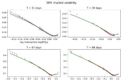
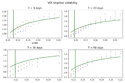
Figure 18: Fractional kernel $K^{frac}$: Joint calibration of SPX implied volatility, VIX implied volatility and VIX futures on 23 October, 2017 using the fractional kernel $K^{frac}$. The blue and red dots are bid/ask implied volatilities, with the green lines are model fit. The vertical bars represents VIX futures price. Calibrated parameters are: $\rho=-1,H=0.09698,(\alpha_{0},\alpha_{1},\alpha_{3},\alpha_{5})=(0.61799,0.90211,1,0.0097)$.

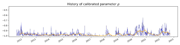
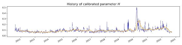
Figure 21: Fractional kernel $K^{frac}$: Evolution of the calibrated parameters $\rho$ and $H$ under the fractional kernel $K^{frac}$, the blue line is the actual value of the calibrated parameters in time, the orange line is the 30-day moving average. Note how $\rho$ is saturated at -1 in most days, but still not enough to capture the SPX ATM skew. $H$ is unable to descent to near zero due to the “vanishing” skew phenomena.

Despite pushing $\rho$ to the boundary value $-1$ in most days (which should increase the SPX ATM skew in stochastic volatility models) as shown in Figure 21 of Appendix B.3, the joint calibrated SPX ATM skew is too flat compared to the market data. The VIX implied volatility produced by the model is generally too high and does not have enough ATM skew, see Figure 18 of Appendix B.2. One can try improving the VIX fit by pushing $H$ closer to zero, but this will further flatten the SPX ATM skew.

The log-modulated kernel

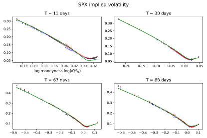
Figure 19: Log modulated kernel $K^{log}$: Joint calibration of SPX implied volatility, VIX implied volatility and VIX futures on 23 October, 2017 using the log modulated kernel $K^{log}$. The blue and red dots are bid/ask implied volatilities, with the green lines are model fit. The vertical bars represents VIX futures price. Calibrated parameters are: $\rho=-0.993822,H=0.01608,\beta=4,(\alpha_{0},\alpha_{1},\alpha_{3},\alpha_{5})=(0.32486,0.0,0.49826,0.017482)$.

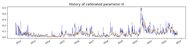
Figure 22: Log modulated kernel $K^{log}$: Evolution of the calibrated parameters $\rho$ and $H$ under the log modulated kernel $K^{log}$, the blue line is the actual value of the calibrated parameters in time, the orange line is the 30-day moving average. Note how $\rho$ is still very close to -1 in most days, while $H$ is much closer to zero than that of fractional kernel $K^{frac}$. In any case, the log modulated kernel $K^{log}$ still struggles to jointly calibrate SPX and VIX.

$K^{log}(t)=\text{max}(\theta\log(1/t),1)^{-\beta},H\in[0,1/2],\theta>0,\beta>1$ is proposed by [12], where $X$ is well-defined even when $H=0$. In [12, Figure 1.1], it is shown that this kernel is capable of resisting the SPX ATM skew flattening suffered by the fractional kernel $K^{frac}$. The calibrated $H$ appears to be just about zero during normal market conditions with a slightly less saturated $\rho$, see Figure 22 of Appendix B.3. The joint fit seems to be slightly better than that of the fractional kernel $K^{frac}$ , see Figure 19 of Appendix B.2.

However, the joint calibration results are still not satisfactory. It seems $H$ needs to go even further below zero (something impossible for the log modulated kernel $K^{log}$ and the fractional kernel $K^{frac}$) to produce the steep VIX ATM skew along with lower level of VIX implied volatility. This motivates the use of the following shifted fractional kernel $K^{{shift}}$.

The shifted fractional kernel

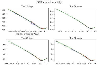
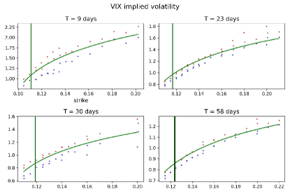
Figure 20: Shifted fractional kernel $K^{shift}$: Joint calibration of SPX implied volatility, VIX implied volatility and VIX futures on 23 October, 2017 using the shifted fractional kernel $K^{shift}$. The blue and red dots are bid/ask implied volatilities, with the green lines are model fit. The vertical bars represents VIX futures price. Calibrated parameters are: $\rho=-0.6891,H=-0.845297,(\alpha_{0},\alpha_{1},\alpha_{3},\alpha_{5})=(0.1035051,0.163729,0.0001054,5.1882e-8)$.

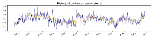
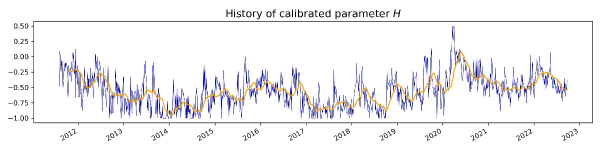
Figure 23: Shifted fractional kernel $K^{shift}$: Evolution of the calibrated parameters $\rho$ and $H$ under the shifted fractional kernel $K^{shift}$, the blue line is the actual value of the calibrated parameters in time, the orange line is the 30-day moving average. Note how $\rho$ is not saturated, similar to that of exponential kernel $K^{exp}$, with $H$ basically staying below zero the entire time series (except during 2020 Covid pandemic).

$K^{shift}(t)=(t+\varepsilon)^{H-1/2}$, for some $\varepsilon>0$, is now well-defined and locally square-integrable for any $H\in(-\infty,1/2]$. The kernel is even smooth enough to make $X$ a semi-martingale but not Markovian, see Proposition 5.2 below. The empirical joint calibration results are considerably better compared to the fractional kernel $K^{frac}$ and the log-modulated kernel $K^{log}$, see Figure 20 of Appendix B.2. The history of calibrated $H$ spends most of its time below zero (except for a brief moment during 2020 Covid pandemic), with $\rho$ no longer saturated and averaging around -0.7, see Figure 23 of Appendix B.3. One issue with this kernel is that $X$ is not Markovian and is path dependent.

The exponential kernel $K^{exp}$.

The choice of the exponential kernel, along with its particular parametrization is motivated as a proxy of the shifted fractional kernel that would yield Markovian dynamics for $X$. To see this, we recall the following representation of the fractional kernel as a Laplace transform:

$$t^{H-1/2} =c_{H}\int_{{\mathbb{R}}_{+}}e^{-xt}{x^{-H-1/2}}dx,$$

with $c_{H}=1/\Gamma(1/2-H)$ and $\Gamma(z):=\int_{{\mathbb{R}}_{+}}x^{z-1}e^{-x}dx$ the Gamma function for $z>0$. We note that such representation as a Laplace transform has been used in the literature to disentangle the (infinite-dimensional) Markovian structure of fractional processes [3, 6, 18, 22, 39] and develop efficient numerical Markovian approximations [1, 7, 9, 38, 58]. For fixed $\varepsilon>0$, the shifted fractional kernel then reads

$$(t+\varepsilon)^{H-1/2} =\int_{{\mathbb{R}}_{+}}e^{-xt}\mu_{H,\varepsilon}(dx){\mbox{w}ith}\quad\mu_{H,\varepsilon}(dx):=c_{H}e^{-x\varepsilon}{x^{-H-1/2}}dx.$$

Now we choose $c_{H,\epsilon}$ and $\gamma_{H,\varepsilon}$ such that the measure $\nu_{H,\varepsilon}(dx)=c_{H,\varepsilon}\delta_{\gamma_{H,\varepsilon}}(dx)$ satisfies

$$\nu_{H,\varepsilon}({\mathbb{R}}_{+})=\mu_{H,\varepsilon}({\mathbb{R}}_{+})\quad\mbox{and}\quad\int_{{\mathbb{R}}_{+}}x\nu_{H,\varepsilon}(dx)=\int_{{\mathbb{R}}_{+}}x\mu_{H,\varepsilon}(dx),$$

with $\delta$ the dirac measure. This yields that

$$c_{H,\varepsilon}=\varepsilon^{H-1/2}\quad\mbox{and}\quad\gamma_{H,\varepsilon}=(1/2-H)\varepsilon^{-1}$$

leading to the following exponential kernel

$$K^{exp}(t):=\int_{{\mathbb{R}}_{+}}e^{-xt}\nu_{H,\varepsilon}(dx)=\varepsilon^{H-1/2}e^{-(1/2-H)\varepsilon^{-1}t}.$$

For small values of $\varepsilon$ and $H$, this parametrisation gives a (Markovian) Ornstein-Uhlenbeck process $X$ in (2.2) with a fast mean reversion of order $(1/2-H)\varepsilon^{-1}$ and a large vol-of-vol of order $\varepsilon^{H-1/2}$ with the following dynamics

$$dX_{t}=-(1/2-H)\varepsilon^{-1}X_{t}dt+\varepsilon^{H-1/2}dW_{t}.$$

It is interesting to note that special cases of such parametrizations of conventional stochastic volatility models have already appeared in the literature but for a fixed value of $H$: for $H=0$ one recovers the fast regimes extensively studied by Fouque et al. [28], see also [27, Section 3.6]; setting $H=-1/2$ yields the parametrization studied by Mechkov [45] and establishes the link with jump models.

Based on empirical results, the exponential kernel $K^{exp}$ produces the best joint fit compared to the other kernels while being the simplest (semi-martingale and Markovian). For SPX maturities up to 3 months and VIX maturities up to 2 months, the exponential kernel $K^{exp}$ can achieve remarkable fits, as shown in Figure 1 of implied volatility surfaces dated 23 October 2017, with calibrated parameters $\rho=-0.6997,H=-0.06939,(\alpha_{0},\alpha_{1},\alpha_{3},\alpha_{5})=(0.82695,0.84388,0.55012,0.03271)$.

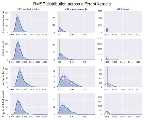
Figure 17: RMSE across different kernels (more details on this).

The historical time series of joint calibration rooted mean square error (RMSE) in Figure 2 and the distribution of the RMSE in Figure 17 of Appendix B.1 show that the exponential kernel $K^{exp}$ outperforms other kernels for all market conditions for both SPX and VIX fit.

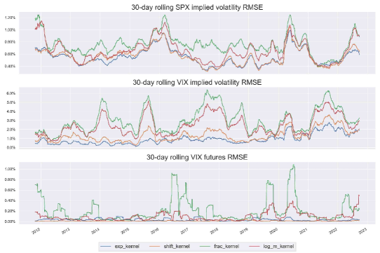
Figure 2: RMSE across different kernels: the exponential kernel $K^{exp}$ outperforms other kernels in all market conditions.

The evolution of jointly calibrated parameters $H$ and $\rho$ also appear to be stable over time in the case of the exponential kernel as shown in Figure 3. This further validates the robustness of the exponential kernel $K^{exp}$ to jointly fit SPX and VIX implied volatilities. Notice that $H$ and $\rho$ also appear to be negatively correlated to one another. We observe that $\rho$ is far from being saturated to $-1$ and $H$ is on average very small and dip below zero from time to time. The parameters $\rho$ and $H$ for the shifted fractional kernel $K^{shift}$ display a similar trend, see Figure 23 of Appendix B.3.

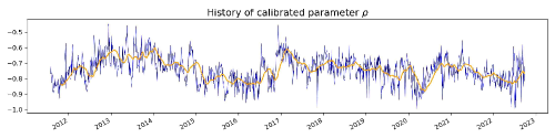
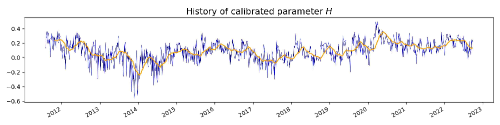
Figure 3: Evolution of the calibrated parameters $\rho$ and $H$ under the exponential kernel $K^{exp}$, the blue line is the actual value of the calibrated parameters in time, the orange line is the 30-day moving average.

For graphs on the joint calibration results by quantiles for the exponential kernel $K^{exp}$, the reader can refer to the Appendix B.4.

4 Fast pricing of VIX derivatives via Quantization

4.1 $L^{2}$-quantization of Gaussian random variables

The idea of quantization is to approximate an $\mathbb{R}$-valued random variable $Y$ with a discrete random variable $\widehat{Y}$ in the computation of ${\mathbb{E}}[F(Y)]$ for some function $F$. Quantization provides a faster alternative to Monte Carlo when no closed form expression of the expectation is available. We will concentrate on the case where $Y$ is Gaussian.

Formally, fix $N\in\mathbb{N}$, for a given set of $N$-points $\Gamma$ given by

$$\Gamma=\{y_{1},\ldots,y_{N}\}\subset\mathbb{R},$$

we consider the Borel partition $C=\{C_{1},\ldots,C_{N}\}$ of $\mathbb{R}$ induced by $\Gamma$ using the nearest neighbourhood projection:

$$C_{i}=\left[y_{i-\frac{1}{2}},y_{i+\frac{1}{2}}\right[,\quad y_{i\pm\frac{1}{2}}:=\frac{y_{i}+y_{i\pm 1}}{2},\quad y_{0}=-\infty,\quad y_{N+1}=\infty,\quad i\in\{1,\ldots,N\}.$$

The $N$-quantizer $\widehat{Y}^{\Gamma}$ is defined by

$$\widehat{Y}^{\Gamma}(\omega)=\sum_{i=1}^{N}y_{i}1_{C_{i}}(Y(\omega))$$ (4.1)

with the associated probability vector $p=\{p_{1},\ldots,p_{N}\}$ such that:

$$p_{i}=\mathbb{Q}(\widehat{Y}^{\Gamma}=y_{i})=\mathbb{Q}(Y\in C_{i})=\int_{y_{i-\frac{1}{2}}}^{y_{i+\frac{1}{2}}}d\mathbb{Q}_{Y}=\mathcal{N}(y_{i+\frac{1}{2}})-\mathcal{N}(y_{i-\frac{1}{2}}),\quad i\in\{1,\ldots,N\},$$ (4.2)

with $\mathcal{N}(x)=\int_{-\infty}^{x}e^{-z^{2}/2}dz/\sqrt{2\pi}$ the cumulative density function of the standard Gaussian distribution. In particular, one can look for the $L^{2}$-optimal $N$-quantizer $\widehat{Y}^{{\Gamma}*}$ with $\Gamma*$ given by

$${{\Gamma}*}=\arg\min_{\Gamma}{\mathbb{E}}\left[\left(Y-\widehat{Y}^{\Gamma}\right)^{2}\right].$$ (4.3)

For standard Gaussian random variable $Y$, the existence and uniqueness of the $L^{2}$-optimal $N$-quantizers have been established in [47], along with a large family of distributions. The $L^{2}$-optimal $N$-quantizer is usually computed numerically, using either a zero search (Newton-Raphson gradient descent) or a fixed point procedure [42, 48]. Optimal quantizers for $N$ up to $5999$ have been computed offline in [50] and are available online at http://www.quantize.maths-fi.com/ in the format of pairs of $(y_{i},p_{i})$.

From now on, we use $\widehat{Y}$ to denote the $L^{2}$-optimal $N$-quantizer $\widehat{Y}^{{\Gamma}*}$ to ease notations. It is now natural to consider the following approximations:

$$\mathbb{E}[F(Y)]\approx\mathbb{E}[F(\widehat{Y})]=\sum_{i=1}^{N}F(y_{i})p_{i}.$$ (4.4)

Such ideas can be extended to approximate the Brownian motion $W$ and the VIX in (2.11). This is the object of the next subsections.

4.2 $L^{2}$-product functional quantization of Brownian motion

Let us now consider the Brownian motion $(W_{t})_{0\leq{t}\leq{T}}$ defined under Section 2. The idea of product functional quantization is to reduce the infinite dimension of the path space of $W$ into finite $N$ number of paths. To do this , we start with the celebrated Karhunen–Loève decomposition of the Brownian motion $W$ in the form of

$$W_{t}=\sum_{k=1}^{\infty}\sqrt{\lambda_{k}}e_{k}{(t)}Y_{k},{\quad 0\leq t\leq T,}$$ (4.5)

with $(Y_{k})_{k\geq 1}$ i.i.d.standard Gaussian and

$$e_{k}(t):=\sqrt{\frac{2}{T}}\sin\left(\pi(k-1/2)\frac{t}{T}\right),\quad\lambda_{k}:=\left(\frac{T}{\pi(k-1/2)}\right)^{2},\quad k\geq 1.$$

More precisely, $(e_{k},\lambda_{k})$ are the $k^{th}$ pair of eigenfunctions in $L^{2}([0,T])$ and positive eigenvalues associated with the covariance kernel ${C_{W}}(t,s)=s\wedge t$:

$$\int_{0}^{T}C_{W}(t,s)e_{k}(s)ds=\lambda_{k}e_{k}(t),\quad k\geq 1,{\quad 0\leq t\leq T}.$$

We note that $(\lambda_{k})_{k\geq 1}$ are decreasing and go to zero as $k$ goes to infinity.

Using (4.5), the product quantization is achieved by 1) truncating the infinite sum to a finite level $m$ and 2) quantizing the i.i.d standard Gaussian $Y_{k}$. For a given $N\in\mathbb{N}$, the product quantizer of the Brownian motion $W$ is defined as follows:

$$\widehat{W}_{t}^{\left(N,m\right)}=\sum_{k=1}^{m}\sqrt{\lambda_{k}}e_{k}{(t)}\widehat{Y}_{k}^{\left(N_{k}\right)},$$ (4.6)

where for each $k\in\{1,\ldots,m\}$, $\widehat{Y}_{k}^{\left(N_{k}\right)}$ is the $L^{2}$-optimal $N_{k}$-quantizer of the standard Gaussian $Y_{k}$ given in Section 4.1 with $N_{k}$ number of quantized points $y^{k}=\{y^{k}_{1},\ldots,y^{k}_{N_{k}}\}$. The product quantizer $\widehat{W}^{(N,m)}$ has (at most) $N$ trajectories, i.e. $N_{1}\times N_{2}\times\ldots\times N_{m}\leq N$. More precisely, for a specific $\omega\in\Omega$, the trajectory of $\widehat{W}_{t}^{(N,m)}$ is defined as:

$$\widehat{W}_{t}^{\left(N,m\right)}(\omega)=\sum_{k=1}^{m}\sqrt{\lambda_{k}}e_{k}{(t)}\sum_{\underline{i}\in\prod_{j=1}^{m}\{1,2,\ldots,N_{j}\}}y_{\underline{i}_{k}}^{k}1_{\{(Y_{1}(\omega),\ldots,Y_{m}(\omega))\in C_{\underline{i}}\}},$$ (4.7)

where $\underline{i}_{k}\in\{1,2,\ldots,N_{k}\}$ denotes the $k$-th element of the tuple $\underline{i}=(\underline{i}_{1},\ldots,\underline{i}_{m})\in\prod_{j=1}^{m}\{1,2,\ldots,N_{j}\}$, with $C_{\underline{i}}$ the partition of $\mathbb{R}^{m}$ defined by

$$C_{\underline{i}}=\prod_{l=1}^{m}\left[y_{\underline{i}_{l}-\frac{1}{2}}^{l},y_{\underline{i}_{l}+\frac{1}{2}}^{l}\right[,\hskip 11.38092pty_{\underline{i}_{l}\pm\frac{1}{2}}^{l}:=\frac{y_{\underline{i}_{l}}^{l}+y_{\underline{i}_{l}\pm 1}^{l}}{2},\hskip 5.69046pty_{0}^{l}=-\infty,\hskip 5.69046pty_{N_{l}+1}^{l}=\infty.$$ (4.8)

In other words, $C_{\underline{i}}$ is a Cartesian grid formed by $m$ number of optimal $L^{2}$-quantized standard Gaussians. Using the independence of the family $(\widehat{Y}_{k}^{(N_{k})})_{k=1,\ldots,m}$, the probability associated with each trajectory $w_{\underline{i}}$ of $\widehat{W}_{t}^{\left(N,m\right)}$, defined as $w_{\underline{i}}=\sum_{k=1}^{m}\sqrt{\lambda_{k}}e_{k}{(t)}y_{\underline{i}_{k}}^{k}$, is straightforward and given by

$$p_{\underline{i}}:=\mathbb{Q}\left(\widehat{W}^{(N,m)}=w_{\underline{i}}\right)=\mathbb{Q}\left(\widehat{Y}^{(N_{k})}_{k}=y_{\underline{i}_{k}}^{k},k\in\{1,\ldots,m\}\right)=\prod_{k=1}^{m}\mathbb{Q}\left(\widehat{Y}^{(N_{k})}_{k}=y_{\underline{i}_{k}}^{k}\right),$$

where we recall that the quantities $\mathbb{Q}(\widehat{Y}^{(N_{k})}_{k}=y_{\underline{i}_{k}})$ appearing on the right hand side are explicitly given by (4.2).

By fixing the number of trajectories $N$ and using the $L^{2}$-optimal $N_{k}$-quantizer $Y_{k}^{(N_{k})}$, the optimal $L^{2}$-product quantizer on the space $\Omega\times[0,T]$ essentially comes down to the trade-off between the choice of $m$ and the sequence $(N_{k})_{k\leq m}$ subject to $\prod_{k=1}^{m}N_{k}\leq N$ by solving the following optimisation problem

$$\min_{\begin{subarray}{c}(N_{k})_{k\leq m},m\geq 1\\ \prod_{k=1}^{m}N_{k}\leq N\end{subarray}}\mathbb{E}\left[\int_{0}^{T}\left(W_{s}-\widehat{W}_{s}^{\left(N,m\right)}\right)^{2}ds\right],$$ (4.9)

with

$$\mathbb{E}\left[\int_{0}^{T}\left(W_{s}-\widehat{W}_{s}^{\left(N,m\right)}\right)^{2}ds\right]=\sum_{k=1}^{m}\lambda_{k}\mathbb{E}\left[\left(Y_{k}-\widehat{Y}_{k}^{\left(N_{k}\right)}\right)^{2}\right]+\sum_{k=m+1}^{\infty}\lambda_{k},$$ (4.10)

using the orthonormality of the eigenfunction $e_{k}$ and independence of $Y_{k}$. Thus, the minimization of the of the error function (4.10) is a balancing act between the $L^{2}$-projection error of individual i.i.d. random variables $Y_{k}$ (intra-class error) and the error of truncation of the KL decomposition (inter-class error). It can be proved, see [47, Theorem 5], that a solution to (4.10) always exists and is unique. The quantizer $\widehat{W}^{(N,m)^{*}}$ with $\{(N_{k})_{k\leq m^{*}}^{*},m^{*}\}$ that solves (4.10) is called the $L^{2}$ (rate) optimal product quantizer. To alleviate notations in the sequel, we will 1) use $\widehat{W}$ to denote the $L^{2}$-optimal product quantizer of $W$, and 2) identify the tuple $\underline{i}$ with a corresponding index $i\in\{1,\ldots,N\}$, so when we mention the $i$-th trajectory of $\widehat{W}$, we are referring to the trajectory $\underline{i}$ generated by the tuple $y_{\underline{i}}=(y_{\underline{i}_{1}}^{1},\ldots,y_{\underline{i}_{m}}^{m},)$, so that

$${w_{i}:=w_{\underline{i}}=\sum_{k=1}^{m}\sqrt{\lambda_{k}}e_{k}{(t)}y_{\underline{i}_{k}}^{k}},\quad N_{1}\times N_{2}\times\ldots\times N_{m}\leq N.$$

In practice, the optimal decomposition sequence $N_{1},\ldots,N_{m}$ are solved numerically using blind optimisation, which consists of computing (4.10) for every possible decomposition $N_{1}\times N_{2}\times\ldots\times N_{m}\leq N$, see [49]. For standard Brownian motions, the optimal decomposition sequence for a wide range of values of $N$ is available online at http://www.quantize.maths-fi.com/. We plot an $L^{2}$-optimal product quantizer $\widehat{W}$ in Figure 4 for an illustration.

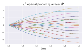
Figure 4: $L^{2}$-optimal product quantizer $\widehat{W}$ of the Brownian Motion, $N=N_{1}\times N_{2}=10\times 2=20$, T = 1.

4.3 VIX derivative pricing via quantization

We recall the explicit expression for the VIX in (2.11) involving the process $Z^{u}_{T}$ in (2.12).

4.3.1 Non-Markovian case

Quantization of $Z_{T}^{u}$.

Fix $T>0$, as done in [17, Section 4], we will use the optimal product quantization $\widehat{W}$ in (4.6) to build a functional quantizer $\widehat{Z}_{T}$ of the process $(Z_{T}^{u})_{u\in[T,T+\Delta]}$ in (2.12) as

$$\widehat{Z}_{T}^{u} =\int_{0}^{T}K(u-s)d\widehat{W}_{s}=\int_{0}^{T}K(u-s)\dot{\widehat{W}}_{s}ds$$ (4.11)

$$=\sum_{k=1}^{m}\sqrt{\lambda_{k}}\widehat{Y}_{k}^{N_{k}}\int_{0}^{T}K(u-s)\dot{e}_{k}(s)ds,\quad\quad\quad u\in[T,T+\Delta],$$ (4.12)

where $\dot{f}$ denotes the derivative of the function $t\mapsto f(t)$.

The quantization of $Z_{T}$ thus requires the computation of the integrals $\left(\int_{0}^{T}K(u-s)\dot{e}_{k}(s)ds\right)_{u\geq T}$ which can be approximated numerically for general kernels. For the fractional kernel $K^{{frac}}$ and shifted fractional kernel $K^{shift}$, recall Table 1, these quantities can be computed explicitly as specified in Appendix A.1. For the log-modulated kernel $K^{{log}}$, we were unable to derive a closed form solution and resorted to using numerical integration techniques to compute $\int_{0}^{T}K(u-s)\dot{e}_{k}(s)ds$ directly (e.g. Gaussian quadrature, which seems to work well in practice).

The quantization of $Z_{T}$ is then straightforward. For a tuple $\text{\text@underline{j}}\in\prod_{i=1}^{m}\{1,2,\ldots,N_{i}\}$, we define $(z_{\underline{j}}^{u})_{u\in[T,T+\Delta]}$ as the $\text{\text@underline{j}}^{\text{th}}$ trajectory of $(\widehat{Z}_{T}^{u})_{u\in[T,T+\Delta]}$, formed through (4.12) in the sense

$$\left(\widehat{Y}^{(N_{k})}_{k}=y_{\underline{j}_{k}}^{k},k\in\{1,\ldots,m\},N_{1}\times N_{2}\times\ldots\times N_{m}\leq N\right)$$

where $y_{\underline{j}_{k}}^{k}$ is the same as those defined in (4.7), with the associated probability given by

$$p_{\underline{j}}=\mathbb{Q}\left(\widehat{Z}_{T}^{u}=z_{\underline{j}}^{u},T\leq u\leq T+\Delta\right)=\prod_{k=1}^{m}\mathbb{Q}\left(\widehat{Y}^{(N_{k})}_{k}=y_{\underline{j}_{k}}^{k}\right)$$

by virtue of the independence of $(\widehat{Y}^{(N_{k})}_{k})_{k=1,\ldots,m}$, where we recall that the quantities appearing on the right hand side are explicitly given by (4.2).

Likewise to the quantized Brownian motion, we ease notations by identifying the tuple $\underline{j}$ with a corresponding index $j\in\{1,\ldots,N\}$, so that $(z_{j}^{u})_{u\in[T,T+\Delta]}$ denotes the $j$-th trajectory of the quantizer $(\widehat{Z}^{u}_{T})_{u\in[T,T+\Delta]}$ with its associated discrete probability $p_{j}{:=p_{\underline{j}}}$.

Quantization of VIX_T.

Once the quantizer $\widehat{Z}_{T}$ is computed, we can plug it in the expression for the VIX in (2.11) to obtain the quantized version $\widehat{\mbox{VIX}}_{T}^{2}$:

$$\widehat{\mbox{VIX}}_{T}^{2}=\frac{100^{2}}{\Delta}\sum_{k=0}^{2M}\sum_{i=0}^{k}(\alpha*\alpha)_{k}{k\choose i}\int_{T}^{T+\Delta}\frac{\xi_{0}(u)}{g(u)}\mathbb{E}\left[(G_{T}^{u})^{i}\right](\widehat{Z}_{T}^{u})^{k-i}du.$$ (4.13)

For $j=1,\ldots,N$, the $j$-th quantized point $v_{j}$ for the $\mbox{VIX}_{T}^{2}$ is explicitly given by

$$v_{j}:=\frac{100^{2}}{\Delta}\sum_{k=0}^{2M}\sum_{i=0}^{k}(\alpha*\alpha)_{k}{k\choose i}\int_{T}^{T+\Delta}\frac{\xi_{0}(u)}{g(u)}\mathbb{E}\left[(G_{T}^{u})^{i}\right](z_{j}^{u})^{k-i}du.$$ (4.14)

Recall that the moments ${\mathbb{E}}[(G^{u}_{T})^{i}]$ are explicitly given by (2.7), so that the integral in (4.14)

$$\int_{T}^{T+\Delta}\frac{\xi_{0}(u)}{g(u)}\mathbb{E}\left[(G_{T}^{u})^{i}\right](z_{j}^{u})^{k-i}(u)du$$

can be approximated efficiently (our numerical implementation shows that $50$ points between $T$ and $T+\Delta$ are largely sufficient using Gaussian quadrature).

With the quantized $\widehat{\mbox{VIX}}_{T}^{2}$, we can now price quickly a variety of VIX derivatives with payoff function $\Phi$ by:

$$\mathbb{E}[\Phi({\mbox{VIX}}_{T})]\approx\mathbb{E}[\Phi(\widehat{\mbox{VIX}}_{T})]=\sum_{j=1}^{N}\Phi(\sqrt{v_{j}})p_{j}.$$ (4.15)

In particular, we can price VIX futures and VIX call options as follows:

$$F_{0}^{\text{\scriptsize VIX}_{T}}=\mathbb{E}[\text{VIX}_{T}]\approx\sum_{j=1}^{N}\sqrt{v_{j}}p_{j},\quad C_{0}^{\text{\scriptsize VIX}_{T}}=\mathbb{E}\left[\left(\mbox{VIX}_{T}-K\right)^{+}\right]\approx\sum_{j=1}^{N}(\sqrt{v_{j}}-K)^{+}p_{j}.$$ (4.16)

The moment-matching trick.

To further improve the accuracy of the VIX pricing via quantization, we propose a moment-matching trick, that is:

$$\tilde{z}_{j}^{u}:=z_{j}^{u}\left(\frac{\mathbb{E}[(Z_{T}^{u})^{q}]}{\sum_{i=1}^{N}(z_{i}^{u})^{q}p_{i}}\right)^{\frac{1}{q}},\quad 1\leq j\leq N,$$ (4.17)

for some even integer $q$ (since $Z_{T}$ has zero odd moments) and for each time step $u\in\left[T,T+\Delta\right]$ and then substitute $\tilde{z}_{j}^{u}$ into (4.14). This way, we can match the $q$-th moment of the quantizer $\widehat{Z}_{T}^{u}$ with that of $Z_{T}^{u}$. We suggest using $q=4$ based on numerical experiments. Note that

$$\mathbb{E}\left[(Z_{T}^{u})^{q}\right]=\left(\int_{u-T}^{u}K^{2}(s)ds\right)^{\frac{q}{2}}(q-1)!!$$ (4.18)

can be computed explicitly for all non-Markovian kernels in this paper for even integer $q$. Figure 5 shows the moment-matching trick results in quantized trajectories being more spread out, and this turns out to speed up convergence in VIX derivative pricing as we will see later.

Figure 5: Comparison of quantizer $\widehat{Z}_{T}^{u}$ using the Volterra fractional kernel $K^{frac}$: LHS is without moment matching, RHS is with moment matching; $T=0.5,H=0.05$, $N=N_{1}\times N_{2}\times N_{3}=10\times 3\times 2=60$.

We stress that such moment matching-trick improves the quality of the quantization considerably, both in terms of VIX future prices and VIX implied volatility smile. Indeed, as shown on Figure 6, quantization without the moment-matching trick is unusable in practice for the fractional kernel with small values of $H$ even with a lot of quantization trajectories $N=100,000$. See also [17, Figure 3], where the number of quantized points were pushed as far as $N=1,000,000$ but the approximation is still well-off the correct values due to the extremely slow convergence rate of the quantization of fractional process in the order of $1/(\log N)^{H}$, see [23]. After moment-matching, we achieve very accurate results with way less quantization points and faster convergence: Figure 7 shows the convergence of VIX pricing using quantization, where $N=200$ seems largely sufficient for pricing and calibrating VIX derivatives! (The Monte Carlo benchmark results are obtained using 6 million simulations with antithetic variables, with total time steps of $50$ between $T$ and $T+\Delta$.)

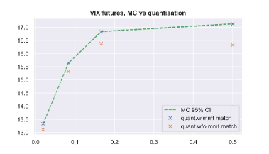
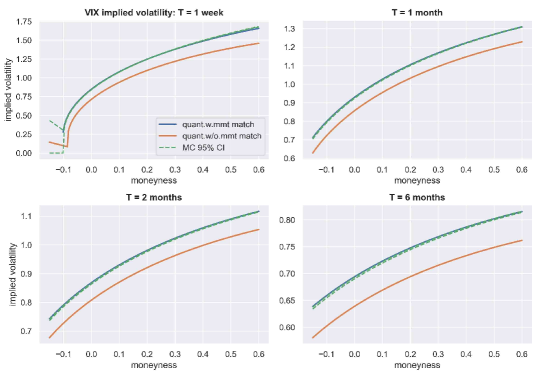
Figure 6: VIX futures term structure and VIX call options implied volatility with $N=100,000$ quantized trajectories of $\widehat{Z}_{T}$ with moment matching (in blue), without moment matching (orange) versus Monte-Carlo prices (dashed green) with $6$ million trajectories and 50 time steps, for the fractional kernel $K^{frac}$ with Hurst index $H=0.05$ and parameters $\xi_{0}(t)=0.005e^{-8t}+0.04(1-e^{-8t})$, $(\alpha_{0},\alpha_{1},\alpha_{3},\alpha_{5})=(0.01,1,0.214,0.227)$.

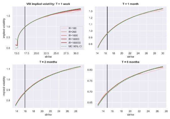
Figure 7: Convergence of the implied volatility of VIX call options using quantization with varying $N$ number of trajectories of $\widehat{Z}_{T}$ under the fractional kernel $K^{frac}$ after moment matching. The Monte-Carlo prices (dashed green) are estimated with $6$ million trajectories and 50 time steps. $H=0.05$, $\xi_{0}(t)=0.03$, $(\alpha_{0},\alpha_{1},\alpha_{3},\alpha_{5})=(0.01,1,0.214,0.227)$.

4.3.2 Markovian case

In the case of the exponential kernel $K^{exp}(t)={\varepsilon^{H-1/2}}e^{-(1/2-H){\varepsilon^{-1}}t}$, the expression of $Z_{T}^{u}$ in (2.12) can be simplified to $Z_{T}^{u}=X_{T}e^{-{(1/2-H)\varepsilon^{-1}}(u-T)}$ with $X_{T}\sim\mathcal{N}\left(0,{\varepsilon^{2H-1}}\frac{1-e^{-(1-2H){\varepsilon^{-1}}T}}{(1-2H){\varepsilon^{-1}}}\right)$. So that VIX_T is just a function of ${\varepsilon^{H-1/2}}\sqrt{\frac{1-e^{-(1-2H){\varepsilon^{-1}}T}}{(1-2H){\varepsilon^{-1}}}}Y$ with $Y$ a standard Gaussian:

$$\mbox{VIX}_{T}^{2} =\frac{100^{2}}{\Delta}\sum_{k=0}^{2M}\sum_{i=0}^{k}(\alpha*\alpha)_{k}{k\choose i}\left({\varepsilon^{H-1/2}}\sqrt{\frac{1-e^{-(1-2H){\varepsilon^{-1}}T}}{(1-2H){\varepsilon^{-1}}}}Y\right)^{k-i}$$ (4.19)

$$\quad\quad\quad\quad\quad\quad\quad\quad\times\int_{T}^{T+\Delta}\frac{\xi_{0}(u)}{g(u)}\mathbb{E}\left[(G_{T}^{u})^{i}\right](e^{-{(1/2-H)\varepsilon^{-1}}(u-T)(k-i)})du.$$ (4.20)

Applying the $L^{2}$-optimal quantizer on $Y$ as in Section 4.1, for $j=1,\ldots,N$, the $j$-th quantized point $v_{j}$ for the $\widehat{\mbox{VIX}}_{T}$ is explicitly given by

$$v_{j} =\frac{100^{2}}{\Delta}\sum_{k=0}^{2M}\sum_{i=0}^{k}y_{j}^{k-i}(\alpha*\alpha)_{k}{k\choose i}{\varepsilon^{(H-1/2)(k-i)}}\left(\frac{1-e^{-(1-2H){\varepsilon^{-1}}T}}{(1-2H){\varepsilon^{-1}}}\right)^{\frac{k-i}{2}}$$ (4.21)

$$\quad\quad\quad\quad\quad\quad\quad\quad\times\int_{T}^{T+\Delta}\frac{\xi_{0}(u)}{g(u)}\mathbb{E}\left[(G_{T}^{u})^{i}\right]e^{-(1/2-H){\varepsilon^{-1}}(u-T)(k-i)}du,$$ (4.22)

where $\{y_{1},\dotsm,y_{N}\}$ are the quantized points of $\widehat{Y}$ with corresponding probabilities $p_{j}=\mathbb{Q}(\widehat{Y}=y_{j})$. The VIX derivatives can then be computed by plugging $(v_{j},p_{j})_{j=1,\ldots,N}$ in the formula (4.15). For the exponential kernel, the convergence is a lot faster after applying a similar moment-matching trick directly on the quantized points of $\widehat{Y}$, with $q$ an even integer:

$$\tilde{y}_{j}:=y_{j}\left(\frac{\mathbb{E}[Y^{q}]}{\sum_{i=1}^{N}(y_{i})^{q}p_{i}}\right)^{\frac{1}{q}},\quad 1\leq j\leq N.$$ (4.23)

Th convergence of VIX pricing using quantization in the Markovian case is shown in Figure 8.

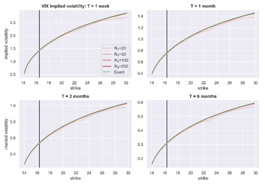
Figure 8: Convergence of the implied volatility of VIX call options using quantization with varying $N$ number of trajectories of $\widehat{Z}_{T}$ under the exponential kernel $K^{exp}$ after moment matching. The dotted green line represents VIX implied volatility calculated by integrating the payoff function of expression (4.20) directly against the Gaussian density. $H=-0.2,\varepsilon=1/52$, $\xi_{0}(\cdot)=0.03$, $(\alpha_{0},\alpha_{1},\alpha_{3},\alpha_{5})=(0.01,1,0.214,0.227)$.

5 Fast pricing of SPX options via Neural Networks with Quantization hints

5.1 Quantization techniques to SPX derivatives

We now explain how to extend the quantization ideas to approximate derivative prices $P_{0}$ on $S$ of the form

$$P_{0}: =\mathbb{E}\left[F(\log(S_{T}))\right],$$ (5.1)

for some payoff function $F$. The process $\log(S)$ in (2.2) reads

$$\log(S_{T})=\log(S_{0})-\frac{1}{2}U_{T}+\rho V_{T}+\sqrt{1-\rho^{2}}V_{T}^{\perp},$$

with

$$U_{T}=\int_{0}^{T}\sigma_{s}^{2}ds,\hskip 5.69046ptV_{T}=\int_{0}^{T}\sigma_{s}dW_{s},\hskip 5.69046ptV_{T}^{\perp}=\int_{0}^{T}\sigma_{s}dW_{s}^{\perp}.$$

We denote by $(\mathcal{F}^{W}_{t})_{t\geq 0}$, the natural filtration generated by the Brownian motion $W$.

Using the celebrated conditioning argument on $\mathcal{F}_{{T}}^{W}$ in stochastic volatility models of [54] combined with the fact that $\mathbb{E}\left[V_{T}^{\perp}\mid\mathcal{F}^{W}_{T}\right]$ is Gaussian with conditional mean zero and conditional variance $U_{T}$, we get

$$P_{0} =\mathbb{E}[F(\log(S_{T}))]$$

$$=\mathbb{E}\left[\mathbb{E}\left[F\left(\log(S_{0})-\frac{1}{2}U_{T}+\rho V_{T}+\sqrt{1-\rho^{2}}\ V_{T}^{\perp}\right){\ \Big{|}\ }\mathcal{F}^{W}_{T}\right]\right]$$

$$=\mathbb{E}\left[\tilde{F}\left(U_{T},V_{T}\right)\right]$$

after applying properties of conditional expectations with the deterministic function $\tilde{F}$:

$$\tilde{F}\left(u,v\right)=\int_{\mathbb{R}}F\left(\log(S_{0})-\frac{1}{2}u+\rho v+\sqrt{(1-\rho^{2})u}z\right)e^{-z^{2}/2}dz/\sqrt{2\pi}.$$

With the help of quantization, we then approximate $P_{0}$ by

$$P_{0}\approx\sum_{j=1}^{N}p_{j}\tilde{F}(u_{j},v_{j})$$

with $(u_{j},v_{j},p_{j})_{1\leq j\leq N}$ the tuple of quantized points of $U_{T}$, $V_{T}$ and their associated discrete probability $p_{j}$ to be defined in the coming sections.

Example 5.1.

For instance, for the case of a European Call option, with payoff $F(x)=(e^{x}-K)^{+}$, we have

$$\tilde{F}(U_{T},V_{T})=\mathcal{BS}^{call}\left(S_{0}\exp\left(-\frac{1}{2}\rho^{2}U_{T}+\rho V_{T}\right),\sqrt{\frac{(1-\rho^{2})U_{T}}{T}},T,K\right)$$

with

$$\mathcal{BS}^{call}(x,\sigma,T,K)=x\mathcal{N}(d_{1})-K\mathcal{N}(d_{2}),$$

$$d_{1}=\frac{\log\left(\frac{x}{K}\right)+\frac{1}{2}\sigma^{2}T}{\sigma\sqrt{T}},\quad d_{2}=d_{1}-\sigma\sqrt{T},$$

with $\mathcal{N}(x)=\int_{-\infty}^{x}e^{-z^{2}/2}dz/\sqrt{2\pi}$ the cumulative density function of standard Gaussian.

With the help of quantization, we price the call by

$$C_{0}\approx\sum_{j=1}^{N}p_{j}\mathcal{BS}^{call}\left(S_{0}\exp\left(-\frac{1}{2}\rho^{2}u_{j}+\rho v_{j}\right),\sqrt{\frac{(1-\rho^{2})u_{j}}{T}},T,K\right).$$ (5.2)

The task now is to quantize the two random variables ($U_{T},V_{T})$.

5.1.1 Quantization of $U_{T}$

Since the path of $U$ is determined by the volatility process $\sigma$, which is itself determined by the path of $X$, the first task is to quantize $X$. Let’s define the quantizer $\widehat{X}$ as:

$$\widehat{X}_{t}=\int_{0}^{t}K(t-s)d\widehat{W}_{s}=\int_{0}^{t}K(t-s)\dot{\widehat{W_{s}}}ds=\sum_{k=1}^{m}\sqrt{\lambda_{k}}\widehat{Y}_{k}^{N_{k}}\int_{0}^{t}K(t-s)\dot{e}_{k}(s)ds.$$ (5.3)

For general kernel $K$, the integral $\int_{0}^{t}K(t-s)\dot{e}_{k}(s)ds$ can be computed numerically (e.g. Gaussian quadrature). For the cases of fractional kernel $K^{frac}$, shifted fractional $K^{shift}$ and exponential kernel $K^{exp}$ this integral can be computed explicitly in Appendix A.2.

Figures 9 and 10 show the quantized trajectories of $\widehat{X}$ under the fractional kernel and exponential kernel for different values of $H$. Recall that the exponential kernel $K^{exp}$ is well-defined for negative values of $H$. Compared to the trajectories of $\widehat{Z}_{T}$ in Figure 5, the trajectories of $\widehat{X}$ seem more “noisy” and tend to cross each other more often.

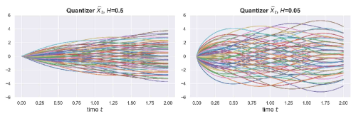
Figure 9: Quantizer $\widehat{X}_{t}$ using the fractional kernel $K^{frac}$, LHS is $H=1/2$, RHS is $H=0.05$; $T=2,N=N_{1}\times N_{2}\times N_{3}=10\times 3\times 2=60$.

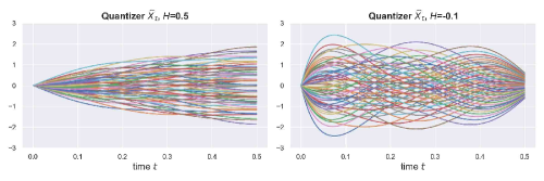
Figure 10: Quantizer $\widehat{X}_{t}$ using the exponential kernel $K^{exp}$, LHS is $H=0.5$, RHS is $H=-0.1$; $\varepsilon=1/52,T=0.5,N=N_{1}\times N_{2}\times N_{3}=10\times 3\times 2=60$.

We now define $(x^{\underline{j}}_{t})_{t\geq 0}$ as the $\underline{j}$-th trajectory at time $t$ of the quantizer $(\widehat{X}_{t})_{t\geq 0}$ in (5.3) with associated probability $p_{\underline{j}}$ as

$$p_{\underline{j}}=\mathbb{Q}\left(\widehat{X}_{t}=x_{t}^{\underline{j}},0\leq t\leq T\right)=\prod_{k=1}^{m}\mathbb{Q}\left(\widehat{Y}^{(N_{k})}_{k}=y_{\underline{j}_{k}}^{k}\right).$$

Again, to ease notations we identify the tuple $\underline{j}$ with a corresponding index $j\in\{1,\ldots,N\}$, so that $(x_{t}^{j})_{t\in[0,T]}$ denotes the $j$-th trajectory of the quantizer $(\widehat{X}_{t})_{t\in[0,T]}$ with its associated discrete probability $p_{j}:=p_{\underline{j}}$.

Define the quantizer $\widehat{\sigma}$ in (2.2) as:

$$\widehat{\sigma}_{t}=\sqrt{\xi_{0}(t)}\frac{p(\widehat{X}_{t})}{\sqrt{{\mathbb{E}}\left[p(X_{t})^{2}\right]}},\quad t\geq 0.\\$$

We are now ready to define the quantizer $\widehat{U}$ as:

$$\widehat{U}_{T}=\int_{0}^{T}\widehat{\sigma}_{s}^{2}ds.$$

This is a Riemann integral, which can be easily computed trajectory by trajectory using numerical integration in the form of:

$$\int_{0}^{T}\widehat{\sigma}_{s}^{2}ds\approx\sum_{p=1}^{n_{T}}\widehat{\sigma}^{2}_{t_{p}}w_{p},$$

for some numerical quadrature methods with weights $w$. For our numerical experiments we used Gaussian quadrature with $n_{T}=50$, but other quadratures are possible. We denote $u_{T}^{j}$ as the $j$-th quantized point of $\widehat{U}_{T}$, with the associated trajectory probability $p_{j}$ carried over directly from the quantizer $\widehat{X}$.

5.1.2 Quantization of $V_{T}$

The quantization of $V_{T}$ is more intricate. In order to understand the intricacy, let us first look at the case where $\sigma$ is a semi-martingale.

Semi-martingale case.

This is the case for smooth enough kernels as shown in the following proposition.

Proposition 5.2.

Assume that $K$ is absolutely continuous on $[0,T]$ with a locally square-integrable derivative $K^{\prime}$. Then, the process

$$X_{t}=\int_{0}^{t}K(t-s)dW_{s}$$

is a semi-martingale with dynamics:

$$dX_{t}=K(0)dW_{t}+\left(\int_{0}^{t}K^{\prime}(t-s)dW_{s}\right)dt.$$

Proof.

Using that $K=K(0)+\int_{0}^{\cdot}K^{\prime}(s)ds$, we obtain

$$X_{t}=K(0)W_{t}+\int_{0}^{t}\int_{0}^{t-s}K^{\prime}(t-s-r)drdW_{s}=K(0)W_{t}+\int_{0}^{t}\int_{0}^{r}K^{\prime}(r-s)dW_{s}dr,$$ (5.4)

where the second equality follows from the stochastic Fubini theorem which applies since $K^{\prime}$ is square-integrable. This ends the proof. ∎

Example 5.3.

The shifted fractional kernel $K^{shift}$ and the exponential kernel $K^{\exp}$ satisfy clearly the assumptions of Proposition 5.2.

Based on the works of Wong and Zakai [57] and Pagès and Sellami [51], we have the convergence of the approximation $\int_{0}^{T}\widehat{\sigma}_{s}d\widehat{W}_{s}$ towards the Stratonovich integral $\int_{0}^{T}\sigma_{s}\circ dW_{s}$:

$$\int_{0}^{T}\widehat{\sigma}_{s}d\widehat{W}_{s}\xrightarrow[N\xrightarrow{}\infty]{}\int_{0}^{T}\sigma_{s}\circ dW_{s}=\int_{0}^{T}\sigma_{s}dW_{s}+\frac{1}{2}\left<\sigma,W\right>_{T},$$ (5.5)

where $\langle\sigma,W\rangle$ is the quadratic covariation between the two semimartingales $\sigma$ and $W$ given by

$$\langle\sigma,W\rangle_{T}=K(0)\int_{0}^{T}\sqrt{\xi_{0}(s)}\frac{p^{\prime}(X_{s})}{\sqrt{\mathbb{E}\left[p(X_{s})^{2}\right]}}ds,\quad p^{\prime}(x)=\sum_{k=0}^{M}k\alpha_{k}x^{k-1}.$$

We therefore construct $\widehat{\left<\sigma,W\right>}_{T}$ as the quantized version of the quadratic covariation as follows:

$$\widehat{\left<\sigma,W\right>}_{T}=K(0)\int_{0}^{T}\sqrt{\xi_{0}(s)}\frac{p^{\prime}(\widehat{X}_{s})}{\sqrt{\mathbb{E}\left[p(X_{s})^{2}\right]}}ds.$$ (5.6)

Using the identity (5.5), we define the $\widehat{V}_{T}$ the quantizer of $V_{T}$ as

$$\widehat{V}_{T}=\int_{0}^{T}\widehat{\sigma}_{s}d\widehat{W}_{s}-\frac{1}{2}\widehat{\left<\sigma,W\right>}_{T}.$$

In practice, the quantizer $\widehat{V}_{T}$ is also computed numerically trajectory by trajectory. Likewise, we denote $v_{T}^{j}$ as the $j$-th trajectory of $\widehat{V}$ at time $T$, with the associated trajectory probability $p_{j}$ carried over directly from quantizer $\widehat{X}$.

Non semi-martingale case.

If the process $(\sigma_{t})_{t\geq 0}$ is not a semimartingale and has infinite quadratic variation, which is the case for the fractional $K^{frac}$ and the log-modulated kernels $K^{log}$ with $H<1/2$: the quadratic covariation $\langle\sigma,W\rangle$ explodes. This can be seen informally on (5.6) since the kernels are singular at $0$, i.e.  $K^{frac}(0)=K^{log}(0)=+\infty$. We suggest the following workaround.

To avoid the explosion in (5.6), we replace $K(0)$ with a positive constant $C$ so that

$$\widehat{\left<\sigma,W\right>}_{T}^{C}=C\int_{0}^{T}\sqrt{\xi_{0}(s)}\frac{p^{\prime}(\widehat{X}_{s})}{\sqrt{\mathbb{E}\left[p(X_{s})^{2}\right]}}ds$$

and thus define the quantizer $\widehat{V}_{T}$ in the non semi-martingale setting as:

$$\widehat{V}_{T}=\int_{0}^{T}\widehat{\sigma}_{s}d\widehat{W}_{s}-\frac{1}{2}\widehat{\left<\sigma,W\right>}_{T}^{C}.$$

A natural choice of $C$ is a value which enforces the centered martingale property of $\widehat{V}_{T}$, i.e. ${\mathbb{E}}\left[\widehat{V}_{T}\right]=0$. That is, we set

$$C=2\frac{{\mathbb{E}}\left[\int_{0}^{T}\widehat{\sigma}_{s}d\widehat{W}_{s}\right]}{\int_{0}^{T}\sqrt{\xi_{0}(s)}\frac{{\mathbb{E}}\left[p^{\prime}(\widehat{X}_{s})\right]}{\sqrt{\mathbb{E}\left[p(X_{s})^{2}\right]}}ds}$$ (5.7)

which can be computed numerically.

It is worth highlighting that $C$ diverges at the limit but acts as renormalization constant. This bears resemblance to the renormalization theory [37] and the approach in [11, Theorem 1.3].

5.1.3 Numerical illustration

For the numerical implementation, we propose two moment-matching tricks to improve convergence. First, we consider the following modified quantizer of $\widehat{W}$:

$$\widetilde{\widehat{W}}_{t}=\sum_{k=1}^{m}\sqrt{\lambda_{k}+\varepsilon_{\lambda}}e_{k}{(t)}\widehat{Y}_{k}^{\left(N_{k}\right)},$$ (5.8)

where $\varepsilon_{\lambda}$ is set to match the trace of the covariance kernel of $X$, that is

$$\mathbb{E}\left[\int_{0}^{T}\widehat{X}_{s}^{2}ds\right]=\mathbb{E}\left[\int_{0}^{T}X_{s}^{2}ds\right]=\int_{0}^{T}\int_{0}^{s}K(u)^{2}duds,$$

with $\widetilde{\widehat{W}}_{t}$ now entering into the definition of the quantizer $\widehat{X}$ in (5.3). The RHS of the integral above can be computed for all kernels in this paper.

The second moment matching trick is to introduce a constant $b$ in front of $\widehat{V}_{T}$ such that

$$\mathbb{E}\left[b\widehat{V}_{T}^{2}\right]=\mathbb{E}\left[\int_{0}^{T}\sigma_{s}^{2}ds=\right]=\int_{0}^{T}\xi_{0}(s)ds,$$

so that the new object $b\widehat{V}_{T}$ now matches both the first and second moments of $V_{T}$.

Figure 11 shows that moment matching improves the quantization results. For $H=1/2$, the moment matching technique produces similar accuracy to that of Romberg interpolation proposed by [47]. However for $H<1/2$, the moment matching tricks outperform Romberg interpolation.

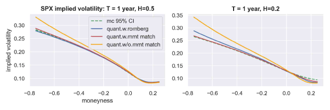
Figure 11: SPX implied volatility smile under the fractional kernel, $\rho=-0.8$, $\alpha=[0,1,0,0,0,0]$, $\xi_{0}(t)=0.02$. The dotted green line ares are Monte Carlo; the blue line is quantisation with Romberg interpolation between $N=1,000$ and $N=10,000$ as per [47]; the red line is quantisation with 10,000 points applying moment matching; the orange line is quantisation with 10,000 points without moment matching. 

Unfortunately, quantization approximation degrade as $H$ goes to zero, as show in Figure 12. In the next section, we will discuss how to use Neural Networks to further improve quantization estimates, especially for lower $H$.

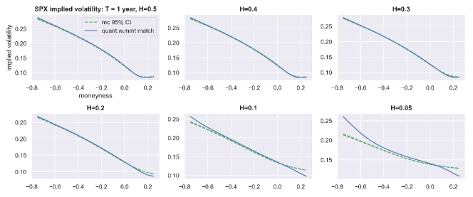
Figure 12: SPX smile under the fractional kernel $K^{frac}$ with different values of $H$, $\rho=-0.8$, $\alpha=[0,1,0,0,0,0]$, $\xi_{0}(t)=0.02$. Green dotted line is Monte Carlo; blue line is quantisation with 10,000 points after moment matching.

5.2 Quantization Neural Network

As we see in Figure 12, the results obtained through quantization degrade as $H$ gets closer to zero for the singular kernels $K^{frac}$ and $K^{log}$. This is also true to some degree for the non-singular kernels $K^{shift}$ and $K^{exp}$ for lower values of $H$. To further improve the estimates on SPX options, we will use Neural Networks.

First, define $n_{\Theta}$ the dimension of the input of the Neural Networks, with $\Theta$ referring to the parameters of the Gaussian polynomial volatility model defined in (3.5) (including the extra parameter $\beta$ for the log-modulated kernel $K^{log}$) together with the maturity parameter $T$, so that $n_{\Theta}=dim(\Theta)+1$. Recall that we fixed $\varepsilon=1/52$ (1 week) for the exponential kernel $K^{exp}$ and time shifted fractional kernel $K^{shift}$, and $\theta=0.1$ for the log-modulated fractional kernel $K^{log}$.

Next, we use Neural Networks (or 3 Neural Networks $\mathcal{NN}^{1},\mathcal{NN}^{2},\mathcal{NN}^{3}$) to modify existing quantized trajectories of $\widehat{X}$ in (5.3) and $d\widetilde{\widehat{W}}$ the derivative of $\widetilde{\widehat{W}}$ in (5.8), as well as to tweak the probability vector $p=(p_{1},\cdots,p_{N})$ by:

$$X^{\mathcal{NN}} =\widehat{X}+\mathcal{NN}^{1},$$ (5.9)

$$dW^{\mathcal{NN}} =d{\widetilde{\widehat{W}}}+\mathcal{NN}^{2},$$

$$p^{\mathcal{NN}} =\text{softmax}(p+\mathcal{NN}^{3}),$$

with the function $\text{softmax}:\mathbb{R}^{N}\rightarrow{(0,1)^{N}},\text{softmax}(r)_{i}=\frac{e^{r_{i}}}{\sum_{j=1}^{N}e^{r_{j}}}$ for $r=(r_{1},\dots,r_{N})\in\mathbb{R}^{N}$, ensuring the output probabilities are positive and sum to $1$. Here, $\widehat{X}$ and $d\widetilde{\widehat{W}}$ are matrices of dimension $N\times n_{T}$ representing the $N$-quantizer with discrete number of time steps $n_{T}$. $\mathcal{NN}$ are Neural Networks such that:

$$\mathcal{NN}^{1},\mathcal{NN}^{2}:\mathbb{R}^{n_{\Theta}}\rightarrow{\mathbb{R}^{N\times n_{T}}}$$

$$\mathcal{NN}^{3}:\mathbb{R}^{n_{\Theta}}\rightarrow{\mathbb{R}^{N}}.$$

At this point, we highlight that the forward variance curves $(\xi_{0}(t))_{t\leq T}$ is not part of the input parameters of the Neural Networks, since we want to tweak the trajectories of $\widehat{X}$, d${\widetilde{\widehat{W}}}$ and the trajectory probabilities so that they remain $\mathbf{independent}$ of the shape of $(\xi_{0}(t))_{t\leq T}$. The treatment of forward variance curves has always been challenging in deep pricing, for example in [40, 55], where a large number of input parameters for the Neural Networks were required to incorporate piece-wise constant forward variance curves. However, our Neural Networks approach solves this problem by 1) using lower input dimension, and 2) generalizing over a larger variety of forward variance curves (e.g. not only piece-wise constant) during training.

5.2.1 Neural Network setup

The input parameters (3.5) (and an extra parameter $\beta$ for the log-modulated kernel $K^{log}$) together with the maturity parameter $T$ are first normalised into the interval $[-1,1]^{n_{\Theta}}$ before feeding into the Neural Networks $\mathcal{NN}$. In terms of Neural Networks’ architecture, we chose 3 hidden layers of 30 neurons each, connected using $tanh(x)=\frac{e^{x}-e^{-x}}{e^{x}+e^{-x}}$ activation function, except for the output layer where identity function is used. The Neural Networks are built using the Tensorflow package in Python.

We then recompute $\widehat{U}_{T}$, $\widehat{V}_{T}$ using $X^{\mathcal{NN}}$ and $dW^{\mathcal{NN}}$. With new quantized points and probabilities $(u_{j}^{\mathcal{NN}},v_{j}^{\mathcal{NN}},p_{j}^{\mathcal{NN}})_{j\leq N}$, we compute the call option price:

$$C(\Theta,T,K)^{\mathcal{NN}}\approx\sum_{j=1}^{N}p_{j}^{\mathcal{NN}}\mathcal{BS}^{call}\left(S_{0}\exp(-\frac{1}{2}\rho^{2}u_{j}^{\mathcal{NN}}+\rho v_{j}^{\mathcal{NN}}),\sqrt{\frac{(1-\rho^{2})u_{j}^{\mathcal{NN}}}{T}},T,K\right).$$ (5.10)

Introducing the following root mean square error:

$$\textbf{RMSE}_{1}=\sqrt{\frac{1}{N_{d}\times M_{k}}\sum_{i=1}^{N_{d}}\sum_{j=1}^{M_{k}}\left(C(\Theta_{i},T_{i},K_{j})^{\mathcal{NN}}-C(\Theta_{i},T_{i},K_{j})^{\mathcal{MC}}\right)^{2}},$$

where $C(\Theta_{i},T_{i},K_{j})^{\mathcal{NN}}$ is the call option priced using $(X^{\mathcal{NN}},dW^{\mathcal{NN}},p^{\mathcal{NN}})$ and $C(\Theta_{i},T_{i},K_{j})^{\mathcal{MC}}$ is the call option priced through Monte Carlo. $N_{d}$ is the number of different ${\Theta}$ in the training dataset and $M_{k}$ is the number of strikes.

It is known that implied volatilities for SPX options are more sensitive to option prices movements for deep out of the money/in the money strikes at shorter maturities. In response, we propose a second loss function which penalises more the regions far away from near the money at shorter maturities:

$$\textbf{RMSE}_{2}=\sqrt{\frac{1}{N_{d}\times M_{k}}\sum_{i=1}^{N_{d}}\sum_{j=1}^{M_{k}}\left(\frac{1}{T_{i}}\log\left(\frac{C(\Theta_{i},T_{i},K_{j})^{\mathcal{NN}}-lb^{call}(K_{j})}{C(\Theta_{i},T_{i},K_{j})^{\mathcal{MC}}-lb^{call}(K_{j})}\right)\right)^{2}},$$

where $lb^{call}(K):=(S_{0}-K)^{+}$ is the theoretical lower bound of a call option in our setting (2.2).

We set the loss function for training the Neural Networks as:

$$\mathcal{L}=\textbf{RMSE}_{1}+\frac{1}{2}\textbf{RMSE}_{2}.$$

Despite the extra computation steps involved between the output of the Neural Networks in (5.9) and the call option price in (5.10), we can capture these computations inside Tensorflow’s computational graph to perform backward propagation to update Neural Networks’ weights. We train the Neural Networks by splitting generated data 85/15 between training and validation set. For each epoch, the training data is divided into mini batches of 200 samples. During the training, Adam Optimiser is used with a learning rate of 0.001 for the first 1,000 epochs, and then a learning rate of 0.0001 for the next 1,000 epochs. More training epochs with smaller learning rates do not improve the results notably, and there appears to be no over fitting by checking the validation error vs.training error, as seen for instance in the case of the exponential kernel $K^{exp}$ in Figure 13 and 14. The distribution of relative errors from the validation dataset seems to be similar to that from training dataset. The relative error is calculated as $|C(\Theta,T,K)^{\mathcal{NN}}-C(\Theta,T,K)^{\mathcal{MC}}|/(C(\Theta,T,K)^{\mathcal{MC}}+\epsilon)$ with $\epsilon=0.1$ to ensure that the errors does not blow up for very small prices in the out of the money region.

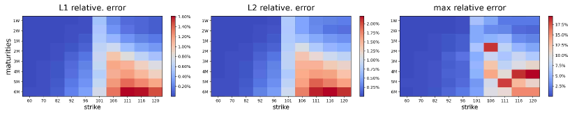
Figure 13: Heatmap of relative errors between estimated prices by Neural Networks vs. Monte Carlo from the validation dataset in the case of exponential kernel $K^{exp}$.

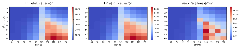
Figure 14: Heatmap of relative errors between estimated prices by Neural Networks vs. Monte Carlo from the training dataset in the case of exponential kernel $K^{exp}$.

Figure 15 shows the improvement of option price estimation via Neural Networks, compared to that of quantization only.

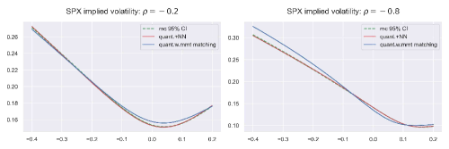
Figure 15: SPX implied volatility smile comparison between Monte Carlo (dotted green lines), quantization only (in blue) and with Neural Networks (in red) with the exponential kernel $K^{exp}$ for different values of $\rho$; $H=-0.1,(\alpha_{0},\alpha_{1},\alpha_{3},\alpha_{5})=(0.001,1,0.1,0.01),T=\text{6 months}$, $\xi_{0}(t)=0.005e^{-8t}+0.04(1-e^{-8t})$. The quantization estimate (in blue) is computed using $10,000$ quantization points, where the quantization + Neural Networks (in red) is based on only $60$ quantization points.

5.2.2 A closed form density function for $\log(S)$

Our approach emits a closed form density function of $\log(S_{T}/S_{0})$, allowing us to price any derivatives depending on the final payoff of spot $S$. To see this, recall that

$$\log(S_{T})=\log(S_{0})-\frac{1}{2}U_{T}+\rho V_{T}+\sqrt{1-\rho^{2}}V_{T}^{\perp}.$$

By modelling $U_{T}$ and $V_{T}$ using quantization, the law of $\log(S_{T}/S_{0})$ is a Gaussian mixture with density function $f(x)$:

$$f(x)=\sum_{j=1}^{N}p_{j}^{\mathcal{NN}}f_{j}(x),$$

where

$$f_{j}(x)=\frac{1}{\sqrt{2\pi(1-\rho^{2})u_{j}^{\mathcal{NN}}}}\exp\left(\frac{-(x+\frac{1}{2}u_{j}^{\mathcal{NN}}-\rho v_{j}^{\mathcal{NN}})^{2}}{2(1-\rho^{2})u_{j}^{\mathcal{NN}}}\right).$$

Figure 16 is an example of density of $\log(S_{T}/S_{0})$ produced by Neural Networks vs. Monte Carlo: the two are very close to each other:

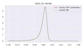
Figure 16: $\log(S_{T}/S_{0})$ density comparison between Monte Carlo (dotted green lines) and Neural Networks (in red) with the exponential kernel $K^{exp}$; $H=-0.1,\rho=-0.8,(\alpha_{0},\alpha_{1},\alpha_{3},\alpha_{5})=(0.001,1,0.1,0.01),T=\text{6 months}$, $\xi_{0}(t)=0.005e^{-8t}+0.04(1-e^{-8t})$.

5.2.3 Data Generation

First, we sample 100,000 different combinations of input parameters for each kernel in this paper as per the following:

$$\rho\sim\mathcal{U}\left[-1,-0.2\right],\left(\alpha_{0},\alpha_{1},\alpha_{3},\alpha_{5}\right)\sim\mathcal{U}\left[0,1\right]^{4},T\sim\mathcal{U}\left[0.01,0.5\right];\beta\sim\mathcal{U}\left[1,4\right],$$

with $\mathcal{U}$ the uniform distribution. For the parameter $H$, we sampled $H\sim\mathcal{U}\left[-1,0.5\right]$ for the exponential kernel $K^{exp}$ and the shifted fractional kernel $K^{shift}$. For the fractional kernel $K^{frac}$ and the log modulated kernel $K^{log}$, we sampled $H\sim\mathcal{U}\left[0.005,0.5\right]$

To sample realistic forward variance curves $(\xi_{0}(t))_{t\leq T}$, we extracted the forward variance curves of SPX between 2017 and 2021 using the celebrated formula by Carr & Madan [19]. To help generalizing the Neural Network to different $(\xi_{0}(t))_{t\leq T}$, we added some noise to the extracted $(\xi_{0}(t))_{t\leq T}$ at each discretised time step $(t_{p})_{1\leq p\leq n_{T}}$ by multiplying $e^{0.2Y_{p}}$ with $(Y_{p})_{1\leq p\leq n_{T}}$ i.i.d. standard Gaussian. This idea is similar to that of [55].

After randomly pairing up the sampled parameters with sampled the forward variance curves, we compute the option call price via Monte Carlo simulations. The process $X$ is simulated exactly using Cholesky decomposition for all kernels. Apart from the covariance matrix of $X$ under the log modulated kernel $K^{log}$ which is computed numerically, all covariance matrices are computed explicitly.

To further reduce MC variance, We make use of antithetic variable for $X$ and the control variable proposed by [14, 44]. The MC prices are computed on a fixed vector of strikes $K:=(K_{1},\ldots,K_{M_{k}})$ ranging between $60\%$ and $120\%$ of spot price $S_{0}=100$. The number of time steps $n_{T}$ is set to $800$ between 0 and $T$ for each simulation, with number of simulations set to $80,000$ including antithetic variables.

5.2.4 Critiques of Neural Networks

Compared to the works of [40, 55, 56], our Neural Networks:

1. learn the joint probability distribution of $(U,V,\log(S))$ instead of learning the map between model parameters $\Theta$ and its implied volatility;

2. do not require a fixed mesh of strikes and maturities and interpolation between various strikes/maturities during joint calibration.

Our approach thus brings several benefits, for instance:

1. Greater flexibility: since the output is a joint density, we can price vanilla options for any strikes and maturities; pricing of other types of derivatives based on the stock price is also possible (transfer learning if needed);

2. Butterfly arbitrage-free: positive density integrating to 1 for $\log(S)$;

3. Improved interpretability: Neural Networks are used as a corrector of a first proxy coming from quantization;

4. Smaller input dimension: the forward variance curve and strikes are not part of the input parameters.

Of course, the price to pay for having a more flexible Neural Networks model is the large number of Neural Networks’ weights involved and longer training time. Recall the output of $\mathcal{NN}^{1}$ and $\mathcal{NN}^{2}$ have dimension of $N\times n_{T}$. As we have set $N=60$ and $n_{T}=50$, the number of weights connecting the last hidden layer and the output layer alone is $(30+1)\times(60\times 50)=93,000$ for $\mathcal{NN}^{1}$ and $\mathcal{NN}^{2}$. Larger $N$ and $n_{T}$ could further improve option prices estimated through Neural Networks, but this will also take longer time to train.

Appendix A Formulae

A.1 A formula for $\int_{0}^{T}(u-s)^{H-1/2}\dot{e}_{k}(s)ds$

Fractional kernel $K^{frac}$:

Thanks to [17], there is a semi-closed form solution for the integral involving the fractional kernel $K^{frac}$:

$$\int_{0}^{T}(u-s)^{H-1/2}\dot{e}_{k}(s)ds=\Bigg{\{}\cos\left(\frac{\left(k-\frac{1}{2}\right)}{T+\Delta}u\pi\right)\left(\zeta_{\frac{1}{2}}\left(\frac{\left(k-\frac{1}{2}\right)}{T+\Delta}u,h_{1}\right)-\zeta_{\frac{1}{2}}\left(\frac{\left(k-\frac{1}{2}\right)}{T+\Delta}(u-T),h_{1}\right)\right)$$

$$+\pi\sin\left(\frac{\left(k-\frac{1}{2}\right)}{T+\Delta}u\pi\right)\left(\zeta_{\frac{3}{2}}\left(\frac{\left(k-\frac{1}{2}\right)}{T+\Delta}u,h_{2}\right)-\zeta_{\frac{3}{2}}\left(\frac{\left(k-\frac{1}{2}\right)}{T+\Delta}(u-T),h_{2}\right)\right)\Bigg{\}}\frac{\sqrt{2}(T+\Delta)^{H}}{\left(k-\frac{1}{2}\right)^{H+\frac{1}{2}}\sqrt{\lambda_{k}}}$$

with $h_{1}=\frac{1}{2}(H+\frac{1}{2})$, $h_{2}=h_{1}+\frac{1}{2}$ and

$$\zeta_{q}(z,h)=\frac{z^{2h}}{2h}\,{}_{1}{F}_{2}(h;q,1+h;\text{-}\frac{1}{4}\pi^{2}z^{2})$$

where ${}_{1}{F}_{2}$ is the hypergeometric function.

Shifted fractional kernel $K^{shift}$:

The formula is similar to the one above for the fractional kernel $K^{frac}$ by simply replacing $u$ by $u+\varepsilon$.

A.2 A formula for $\int_{0}^{t}(t-s)^{H-1/2}\dot{e}_{k}(s)ds$

Fractional kernel $K^{frac}$:

Thanks to [17], there is a semi-closed form solution for the integral involving the fractional kernel $K^{frac}$:

$$\int_{0}^{t}(t-s)^{H-1/2}\dot{e}_{k}(s)ds=\frac{2}{1+2H}\sqrt{\frac{2}{T\lambda_{k}}}t^{H+1/2}{}_{2}{F}_{1}(1;\frac{3}{4}+\frac{H}{2},\frac{5}{4}+\frac{H}{4};-\frac{t^{2}}{4\lambda_{k}}).$$

Shifted fractional kernel $K^{shift}$:

$$\int_{0}^{t}(t+\varepsilon-s)^{H-1/2}\dot{e}_{k}(s)ds=\Bigg{\{}\cos\left(\frac{\left(k-\frac{1}{2}\right)}{T}(t+\varepsilon)\pi\right)\left(\zeta_{\frac{1}{2}}\left(\frac{\left(k-\frac{1}{2}\right)}{T}(t+\varepsilon),h_{1}\right)-\zeta_{\frac{1}{2}}\left(\frac{\left(k-\frac{1}{2}\right)}{T}\varepsilon,h_{1}\right)\right)$$

$$+\pi\sin\left(\frac{\left(k-\frac{1}{2}\right)}{T}(t+\varepsilon)\pi\right)\left(\zeta_{\frac{3}{2}}\left(\frac{\left(k-\frac{1}{2}\right)}{T}(t+\varepsilon),h_{2}\right)-\zeta_{\frac{3}{2}}\left(\frac{\left(k-\frac{1}{2}\right)}{T}\varepsilon,h_{2}\right)\right)\Bigg{\}}\frac{\sqrt{2}t^{H}}{\left(k-\frac{1}{2}\right)^{H+\frac{1}{2}}\sqrt{\lambda_{k}}}$$

with $h_{1}=\frac{1}{2}(H+\frac{1}{2})$, $h_{2}=h_{1}+\frac{1}{2}$ and

$$\zeta_{q}(z,h)=\frac{z^{2h}}{2h}\,{}_{1}{F}_{2}(h;q,1+h;\text{-}\frac{1}{4}\pi^{2}z^{2})$$

where ${}_{1}{F}_{2}$ is the hypergeometric function.

Exponential kernel $K^{exp}$:

the form solution for the integral involving the exponential kernel:

$$\int_{0}^{t}K(t-s)\dot{e}_{k}(s) =\int_{0}^{t}\varepsilon^{H-1/2}e^{-(1/2-H)\varepsilon^{-1}(t-s)}\dot{e}_{k}(s)ds$$

$$=\varepsilon^{H-1/2}\sqrt{\frac{2}{T}}\frac{-(1/2-H)\varepsilon^{-1}e^{-(1/2-H)\varepsilon^{-1}t}+(1/2-H)\varepsilon^{-1}\cos(\frac{t}{\sqrt{\lambda_{k}}})+\frac{1}{\sqrt{\lambda_{k}}}\sin{\frac{t}{\lambda_{k}}}}{((1/2-H)^{2}\varepsilon^{-2}+\frac{1}{\lambda_{k}})\sqrt{\lambda_{k}}}.$$

Appendix B More joint calibration results

B.1 RMSE across different kernels after calibration

B.2 Joint calibration among other kernels for the date 23 October 2017

B.3 Evolution of calibrated parameters under different kernels

B.4 Exponential kernel $K^{exp}$ fit quality quantiles

0.3 Quantile:

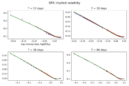
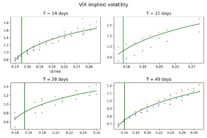
Figure 24: Exponential kernel $K^{exp}$: Joint calibration of SPX implied volatility, VIX implied volatility and VIX futures on 03 April, 2019. The blue and red dots are bid/ask implied volatilities, the green lines are model fit. The vertical bars represents VIX futures price. Calibrated parameters are: $\rho=-0.69148,H=0.04743,(\alpha_{0},\alpha_{1},\alpha_{3},\alpha_{5})=(1,0.1,0.30223,0.04788)$.

0.6 Quantile:

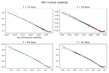
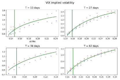
Figure 25: Exponential kernel $K^{exp}$: Joint calibration of SPX implied volatility, VIX implied volatility and VIX futures on 21 July, 2016. The blue and red dots are bid/ask implied volatilities, the green lines are model fit. The vertical bars represents VIX futures price. Calibrated parameters are: $\rho=-0.72793,H=0.1373,(\alpha_{0},\alpha_{1},\alpha_{3},\alpha_{5})=(0.81221,0.73015,0.94968,0.02753)$.

0.99 Quantile:

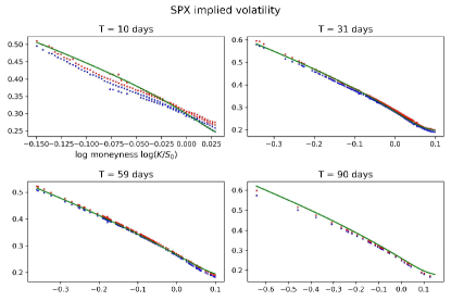
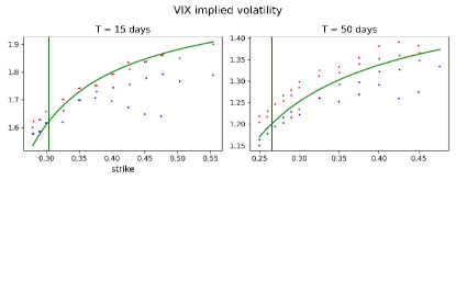
Figure 26: Exponential kernel $K^{exp}$: Joint calibration of SPX implied volatility, VIX implied volatility and VIX futures on 01 September, 2015. The blue and red dots are bid/ask implied volatilities, the green lines are model fit. The vertical bars represents VIX futures price. Calibrated parameters are: $\rho=-0.8171,H=0.35267,(\alpha_{0},\alpha_{1},\alpha_{3},\alpha_{5})=(0.3021,0.8658,0.8522,0.0574)$.

References

- Abi Jaber [2019] Eduardo Abi Jaber. Lifting the Heston model. Quantitative Finance, 19(12):1995–2013, 2019.
- Abi Jaber [2022] Eduardo Abi Jaber. The characteristic function of gaussian stochastic volatility models: an analytic expression. Finance and Stochastics, pages 1–37, 2022.
- Abi Jaber and El Euch [2019a] Eduardo Abi Jaber and Omar El Euch. Markovian structure of the Volterra Heston model. Statistics & Probability Letters, 149:63–72, 2019a.
- Abi Jaber and El Euch [2019b] Eduardo Abi Jaber and Omar El Euch. Multifactor approximation of rough volatility models. SIAM Journal on Financial Mathematics, 10(2):309–349, 2019b.
- Abi Jaber et al. [2019] Eduardo Abi Jaber, Martin Larsson, and Sergio Pulido. Affine volterra processes. The Annals of Applied Probability, 29(5):3155–3200, 2019.
- Abi Jaber et al. [2021] Eduardo Abi Jaber, Enzo Miller, and Huyên Pham. Linear-quadratic control for a class of stochastic volterra equations: solvability and approximation. The Annals of Applied Probability, 31(5):2244–2274, 2021.
- Alfonsi and Kebaier [2021] Aurélien Alfonsi and Ahmed Kebaier. Approximation of stochastic volterra equations with kernels of completely monotone type. arXiv preprint arXiv:2102.13505, 2021.
- Baldeaux and Badran [2014] Jan Baldeaux and Alexander Badran. Consistent modelling of vix and equity derivatives using a 3/2 plus jumps model. Applied Mathematical Finance, 21(4):299–312, 2014.
- Bayer and Breneis [2021] Christian Bayer and Simon Breneis. Makovian approximations of stochastic volterra equations with the fractional kernel. arXiv preprint arXiv:2108.05048, 2021.
- Bayer et al. [2016] Christian Bayer, Peter Friz, and Jim Gatheral. Pricing under rough volatility. Quantitative Finance, 16(6):887–904, 2016.
- Bayer et al. [2020] Christian Bayer, Peter K Friz, Paul Gassiat, Jorg Martin, and Benjamin Stemper. A regularity structure for rough volatility. Mathematical Finance, 30(3):782–832, 2020.
- Bayer et al. [2021] Christian Bayer, Fabian A Harang, and Paolo Pigato. Log-modulated rough stochastic volatility models. SIAM Journal on Financial Mathematics, 12(3):1257–1284, 2021.
- Bennedsen et al. [2021] Mikkel Bennedsen, Asger Lunde, and Mikko S Pakkanen. Decoupling the Short- and Long-Term Behavior of Stochastic Volatility. Journal of Financial Econometrics, 01 2021.
- Bergomi [2015] Lorenzo Bergomi. Stochastic volatility modeling. CRC press, 2015.
- Bergomi and Guyon [2012] Lorenzo Bergomi and Julien Guyon. Stochastic volatility’s orderly smiles. Risk, 25(5):60, 2012.
- Bondi et al. [2022] Alessandro Bondi, Sergio Pulido, and Simone Scotti. The rough hawkes heston stochastic volatility model. arXiv preprint arXiv:2210.12393, 2022.
- Bonesini et al. [2021] Ofelia Bonesini, Giorgia Callegaro, and Antoine Jacquier. Functional quantization of rough volatility and applications to the vix. arXiv preprint arXiv:2104.04233, 2021.
- Carmona and Coutin [1998] Philippe Carmona and Laure Coutin. Fractional brownian motion and the markov property. Electronic Communications in Probability, 3:95–107, 1998.
- Carr and Madan [2001] Peter Carr and Dilip Madan. Towards a theory of volatility trading. Option Pricing, Interest Rates and Risk Management, Handbooks in Mathematical Finance, 22(7):458–476, 2001.
- [20] CBOE. Volatility index methodology: Cboe volatility index. White paper. URL https://cdn.cboe.com/api/global/us_indices/governance/Volatility_Index_Methodology_Cboe_Volatility_Index.pdf.
- Cont and Kokholm [2013] Rama Cont and Thomas Kokholm. A consistent pricing model for index options and volatility derivatives. Mathematical Finance: An International Journal of Mathematics, Statistics and Financial Economics, 23(2):248–274, 2013.
- Cuchiero and Teichmann [2020] Christa Cuchiero and Josef Teichmann. Generalized feller processes and markovian lifts of stochastic volterra processes: the affine case. Journal of evolution equations, 20(4):1301–1348, 2020.
- Dereich and Scheutzow [2006] Steffen Dereich and Michael Scheutzow. High resolution quantization and entropy coding for fractional brownian motion. Electronic Journal of Probability, 11:700–722, 2006.
- El Euch and Rosenbaum [2019] Omar El Euch and Mathieu Rosenbaum. The characteristic function of rough heston models. Mathematical Finance, 29(1):3–38, 2019.
- Forde et al. [2020] Martin Forde, Masaaki Fukasawa, Stefan Gerhold, and Benjamin Smith. The rough bergomi model as h→ 0–skew flattening/blow up and non-gaussian rough volatility. preprint, 2020.
- Fouque and Saporito [2018] J-P Fouque and Yuri F Saporito. Heston stochastic vol-of-vol model for joint calibration of vix and s&p 500 options. Quantitative Finance, 18(6):1003–1016, 2018.
- Fouque et al. [2000] Jean-Pierre Fouque, George Papanicolaou, and K Ronnie Sircar. Derivatives in financial markets with stochastic volatility. Cambridge University Press, 2000.
- Fouque et al. [2003] Jean-Pierre Fouque, George Papanicolaou, Ronnie Sircar, and Knut Solna. Multiscale stochastic volatility asymptotics. Multiscale Modeling & Simulation, 2(1):22–42, 2003.
- Gatheral et al. [2018] Jim Gatheral, Thibault Jaisson, and Mathieu Rosenbaum. Volatility is rough. Quantitative finance, 18(6):933–949, 2018.
- Gatheral et al. [2020] Jim Gatheral, Paul Jusselin, and Mathieu Rosenbaum. The quadratic rough heston model and the joint s&p 500/vix smile calibration problem. arXiv preprint arXiv:2001.01789, 2020.
- Gersho and Gray [2012] Allen Gersho and Robert M Gray. Vector quantization and signal compression, volume 159. Springer Science & Business Media, 2012.
- Goutte et al. [2017] Stéphane Goutte, Amine Ismail, and Huyên Pham. Regime-switching stochastic volatility model: estimation and calibration to vix options. Applied Mathematical Finance, 24(1):38–75, 2017.
- Graf and Luschgy [2000] Siegfried Graf and Harald Luschgy. Foundations of quantization for probability distributions. Foundations Of Quantization For Probability Distributions, 1730:1–+, 2000.
- Grzelak [2022] Lech A Grzelak. On randomization of affine diffusion processes with application to pricing of options on vix and s&p 500. arXiv preprint arXiv:2208.12518, 2022.
- Guo et al. [2022] Ivan Guo, Gregoire Loeper, Jan Obloj, and Shiyi Wang. Joint modeling and calibration of spx and vix by optimal transport. SIAM Journal on Financial Mathematics, 13(1):1–31, 2022.
- Guyon and Lekeufack [2022] Julien Guyon and Jordan Lekeufack. Volatility is (mostly) path-dependent. Volatility Is (Mostly) Path-Dependent (July 27, 2022), 2022.
- Hairer [2014] M Hairer. A theory of regularity structures. Inventiones Mathematicae, 198(2):269, 2014.
- Harms [2019] Philipp Harms. Strong convergence rates for markovian representations of fractional brownian motion, 2019.
- Harms and Stefanovits [2019] Philipp Harms and David Stefanovits. Affine representations of fractional processes with applications in mathematical finance. Stochastic Processes and their Applications, 129(4):1185–1228, 2019.
- Horvath et al. [2021] Blanka Horvath, Aitor Muguruza, and Mehdi Tomas. Deep learning volatility: a deep neural network perspective on pricing and calibration in (rough) volatility models. Quantitative Finance, 21(1):11–27, 2021.
- Isserlis [1918] Leon Isserlis. On a formula for the product-moment coefficient of any order of a normal frequency distribution in any number of variables. Biometrika, 12(1/2):134–139, 1918.
- Kieffer [1982] J Kieffer. Exponential rate of convergence for lloyd’s method i. IEEE Transactions on Information Theory, 28(2):205–210, 1982.
- Kokholm and Stisen [2015] Thomas Kokholm and Martin Stisen. Joint pricing of vix and spx options with stochastic volatility and jump models. The Journal of Risk Finance, 2015.
- McCrickerd and Pakkanen [2018] Ryan McCrickerd and Mikko S Pakkanen. Turbocharging monte carlo pricing for the rough bergomi model. Quantitative Finance, 18(11):1877–1886, 2018.
- Mechkov [2015] Serguei Mechkov. Fast-reversion limit of the heston model. Available at SSRN 2418631, 2015.
- Pacati et al. [2018] Claudio Pacati, Gabriele Pompa, and Roberto Renò. Smiling twice: the heston++ model. Journal of Banking & Finance, 96:185–206, 2018.
- Pages [2008] Gilles Pages. Quadratic optimal functional quantization of stochastic processes and numerical applications. Monte Carlo and Quasi-Monte Carlo Methods 2006, pages 101–142, 2008.
- Pagès and Printems [2003] Gilles Pagès and Jacques Printems. Optimal quadratic quantization for numerics: the gaussian case. 2003.
- Pagès and Printems [2005] Gilles Pagès and Jacques Printems. Functional quantization for numerics with an application to option pricing. 2005.
- [50] Gilles Pagès and Jacques Printems. http://www.quantize.maths-fi.com, 2005. Website devoted to optimal quantization.
- Pagès and Sellami [2011] Gilles Pagès and Afef Sellami. Convergence of multi-dimensional quantized sde’s. In Séminaire de probabilités XLIII, pages 269–307. Springer, 2011.
- Papanicolaou and Sircar [2014] Andrew Papanicolaou and Ronnie Sircar. A regime-switching heston model for vix and s&p 500 implied volatilities. Quantitative Finance, 14(10):1811–1827, 2014.
- Pham and Printems [2004] Huyên Pham and Jacques Printems. Optimal quantization methods and applications to numerical problems in finance. In Handbook of computational and numerical methods in finance, pages 253–297. Springer, 2004.
- Renault and Touzi [1996] Eric Renault and Nizar Touzi. Option hedging and implied volatilities in a stochastic volatility model 1. Mathematical Finance, 6(3):279–302, 1996.
- Rømer [2022] Sigurd Emil Rømer. Empirical analysis of rough and classical stochastic volatility models to the spx and vix markets. Quantitative Finance, 22(10):1805–1838, 2022.
- Rosenbaum and Zhang [2021] Mathieu Rosenbaum and Jianfei Zhang. Deep calibration of the quadratic rough heston model. arXiv preprint arXiv:2107.01611, 2021.
- Wong and Zakai [1965] Eugene Wong and Moshe Zakai. On the convergence of ordinary integrals to stochastic integrals. The Annals of Mathematical Statistics, 36(5):1560–1564, 1965.
- Zhu et al. [2021] Qinwen Zhu, Grégoire Loeper, Wen Chen, and Nicolas Langrené. Markovian approximation of the rough bergomi model for monte carlo option pricing. Mathematics, 9(5):528, 2021.