Robust modeling and inference of disease transmission using error-prone data with application to SARS-CoV-2

Abstract

Modeling disease transmission is important yet challenging during a pandemic. It is not only critical to study the generative nature of a virus and understand the dynamics of transmission that vary by time and location but also crucial to provide accurate estimates that are robust to the data errors and model assumptions due to limited understanding of the new virus. We bridged the epidemiology of pathogens and statistical techniques to propose a hybrid statistical-epidemiological model so that the model is generative in nature yet utilizes statistics to model the effect of covariates (e.g., time and interventions), stochastic dependence, and uncertainty of data. Our model considers disease case counts as random variables and imposes moment assumptions on the number of secondary cases of existing infected individuals at the time since infection. Under the quasi-score framework, we built an “observation-driven model” to model the serial dependence and estimate the effect of covariates, with the capability of accounting for errors in the data. We proposed an online estimator and an effective iterative algorithm to estimate the instantaneous reproduction number and covariate effects, which provide a close monitoring and dynamic forecasting of disease transmission under different conditions to support policymaking at the community level.

Authors’ Footnote: Jiasheng Shi is Post Doctoral Fellow, Department of Biostatistics, Epidemiology, and Informatics, Perelman School of Medicine, University of Pennsylvania, Philadelphia, PA 19104, USA (Jiasheng.Shi@Pennmedicine.upenn.edu). Jeffrey S. Morris is Professor and Division Director, Department of Biostatistics, Epidemiology, and Informatics, Perelman School of Medicine, University of Pennsylvania, Philadelphia, PA 19104, USA (Jeffrey.Morris@pennmedic-
ine.upenn.edu). David M. Rubin is Professor and Director, PolicyLab, Children’s Hospital of Philadelphia, Philadelphia, PA 19104, USA (rubin@chop.edu). Jing Huang is Assistant Professor, Department of Biostatistics, Epidemiology, and Informatics, Perelman School of Medicine, University of Pennsylvania, Philadelphia, PA 19104, USA (Jing14@Pennmedicine.upenn.edu).

Keywords: instantaneous reproduction number; observation-driven model; online estimator; quasi-score method; time-since-infection model

1 Introduction

The onset of the global pandemic of coronavirus disease 2019 (COVID-19), caused by the novel severe acute respiratory syndrome coronavirus 2 (SARS-CoV-2), elevated the importance of modeling and inference of disease transmission. However, both the classic epidemiological framework and modern statistical models for infectious diseases face challenges for modeling transmission and supporting decision making during a pandemic.

First, the classic mathematical epidemiological models provide a basic infrastructure and interpretable estimates to understand the generative nature of a virus but have limited ability to answer extended questions beyond virus generation that are important for decision making. In epidemiological studies, the transmission of an infectious pathogen is estimated by the reproduction number, $R$, which represents the average number of people that will be infected by an individual who has the infection. Many mathematical epidemiological models have been proposed to estimate $R$, including models to estimate the static basic reproduction number $R_{0}$ and the time-varying reproduction number. The $R_{0}$ is a constant representing the average spread potential of the virus over a long period of time in a fully susceptible population, while the time-varying reproduction number measures the disease transmission at a specific time, which is more useful for understanding the dynamics of transmission during a pandemic. The time-varying reproduction number has multiple definitions based on different epidemiological models, including the effective reproduction number (Wallinga and Teunis, 2004), instantaneous reproduction number (Fraser, 2007), case reproduction number (Fraser, 2007), and the reproduction number of time-dependent susceptible-infected-recovered (SIR) Models (Chen et al., 2020), (Song et al., 2020), (Boatto et al., 2018). Most of these existing definitions are based on two basic model frameworks, the SIR ordinary differential equations model and the time-since-infection (TSI) model, both of which are originated from the classic paper of Kermack and McKendrick (1927) and are known as “the Kermack-McKendrick models”.

During the COVID-19 pandemic, many models were introduced purely based on these classic epidemiological models to estimate the transmission of SARS-CoV-2 (Wang et al., 2020; Pan, Liu, Wang, Guo, Hao, Wang, Huang, He, Yu, Lin et al., 2020; Tian et al., 2020; Zhou et al., 2020). These models provided estimates of reproduction numbers but had limited ability to evaluate the effect of control policies or the impact of risk factors. Specifically, the evolution of a new outbreak is driven by multiple factors that almost certainly vary by time and location, including socio-behavioral, environmental and biological factors (Rubin et al., 2020). Policymakers also need to vary their control measures based on the current status of the outbreak as well as time-varying/invariant local factors. These control measures may also have unintended consequences on global economy and human health. To optimize the decision making, it is important to evaluate the benefit and harm of control strategies adjusting for local factors and many other variables.

On the other hand, modern statistical or computational models, while possess a great flexibility to capture the complex shape of disease curve, e.g. time series models (IHME COVID-19 forecasting team, 2020; Pan, Shen and Hu, 2020) and machine learning models for curve data (Dayan et al., 2021; Punn et al., 2020; Ardabili et al., 2020), also have limited use to support decision making due to the lack of epidemiological interpretations of parameters. Therefore, the study results from these models may not be directly used to support decision making either.

In addition to the limitation of models, poor data quality collected during a pandemic can also bias study results and mislead decision making for both the epidemiological and statistical models. Data collection is labor intensive and, for health departments, it can be challenging to stay on top of the numbers across counties due to the lack of shared standards for reporting data, different definitions of diseased individual, varying testing strategies and limited capacity of testing incident cases (Costa-Santos et al., 2021; Sáez et al., 2021). Moreover, models that rely on strong statistical assumptions could further suffer from model mis-specification or failure to include important variables. To better support decision making, it is urgent to build a model with interpretable and accurate estimates that characterize the dynamics of transmission and, more importantly, robust to errors in data and model assumptions.

Motivated from these challenges, we propose a model to bridge the epidemiological modeling of pathogens and flexibility of statistical modeling, and utilize statistical techniques to improve the model robustness. Our proposed model combines the benefits of both the classic epidemiological models and modern statistical models, so that the model is generative in nature yet flexible to model the stochastic dependence of daily transmission, effect of local factors, and errors of data. Specifically, our model forms a two-layer hierarchical structure. On the first layer, we characterize the disease transmission using the instantaneous reproduction number of the TSI model, denoted as $\{R_{t}\}_{t\geq 0}$, by assuming the infectiousness of a diseased individual depends on the time since infection. On the second layer, we build a time series regression model to model correlation between daily transmission and characterize the impact of control measures and local factors. Under a quasi-score framework, we utilize an error term to correct bias due to errors in the data and model mis-specification. To fully characterize the real time impact of local area factors on disease transmission, we proposed an online estimator for $R_{t}$, and constructed an effective iterative algorithm to simultaneously estimate $R_{t}$ and effects of covariates. A regression model based on the TSI model was recently proposed by Quick et al. (2021). The contribution of our work is different from theirs. Quick et al. (2021) tackled case under-ascertainment using additional data resources, e.g. serological surveys and testing metrics, which might not be available in some regions or at the beginning of a pandemic. In our model, the bias due to errors in the data is handled using an error term while data used in our model, e.g. the case incidence data and geographical variables, are largely available across the country during a pandemic. In addition, we focus on building a robust estimation and predictive procedure under fewer model assumptions.

The rest of the paper is organized as follows. We introduce the TSI model and notations in Section 2, followed by description of the proposed model in Section 3. In section 4, we present the asymptotic results and property of estimating procedure under a special case. We show a robust performance of our method in simulation in Section 5, an application to COVID-19 data in Section 6 and a miscellany of discussions in Section 7. Proofs for theoretical properties are shown in the supplementary material.

2 The time-since-infection Model and Generative Nature of a Virus

The TSI model assumes that infectiousness of an infected individual depends on the time since infection. Let $\beta(t,s)$ denote the effective contact rate at time $t$ between susceptible individuals and an infected individual who was infected $s$ time ago, indicating the number of secondary cases that an infected individual can generate at time $t$. The total number of new cases in the population infected at time $t$, denoted as $I_{t}$, can be written as a function of the effective contact rate at time $t$ and the number of all existing cases that were infected before time $t$, i.e. $\mathbbm{E}(I_{t})=\mathbbm{E}\int^{t}_{0}\beta(t,s)I_{t-s}ds$. The instantaneous reproduction number, $R_{t}$, which measures how many secondary infections can be generated from someone infected at time $t$ could expect to infect if conditions remain unchanged, is defined as $R_{t}=\int^{t}_{0}\beta(t,s)ds.$ $\beta(t,s)$ varies as the time since infection $s$ changes, which typically reflects the change of pathogen shedding since infection. In microbiology, it has been found that pathogen shedding is an important determinant for disease transmission (Cevik et al., 2021). If we assume that the change of $\beta(t,s)$ as a function of time since infection $s$ is independent of calendar time $t$, then the $\beta(t,s)$ can be decomposed as $\beta(t,s)=R_{t}\omega_{s}$. Here $\omega_{s}$ is the infectiousness function, measuring infectiousness at the time since infection $s$, with $\int_{0}^{\infty}\omega_{s}ds=1$, and $\omega_{s}=0$ for $s=0$ and $s\geq\eta$ with $\eta$ being the time to recovery since infection. Figure 1 shows an example of the infectiousness function at day $s$ since infection, $\omega_{s}$, approximated using the density function of a gamma distribution with shape and rate parameters equals to 2.5 and 0.255 respectively. The shape of this $\omega_{s}$ over time assumes that the infectiousness of an infected individual increases during the first 7 days since infection as viral loads increase soon after infection and then gradually decrease as the individual proceeds to recovery around 21 days after infection.

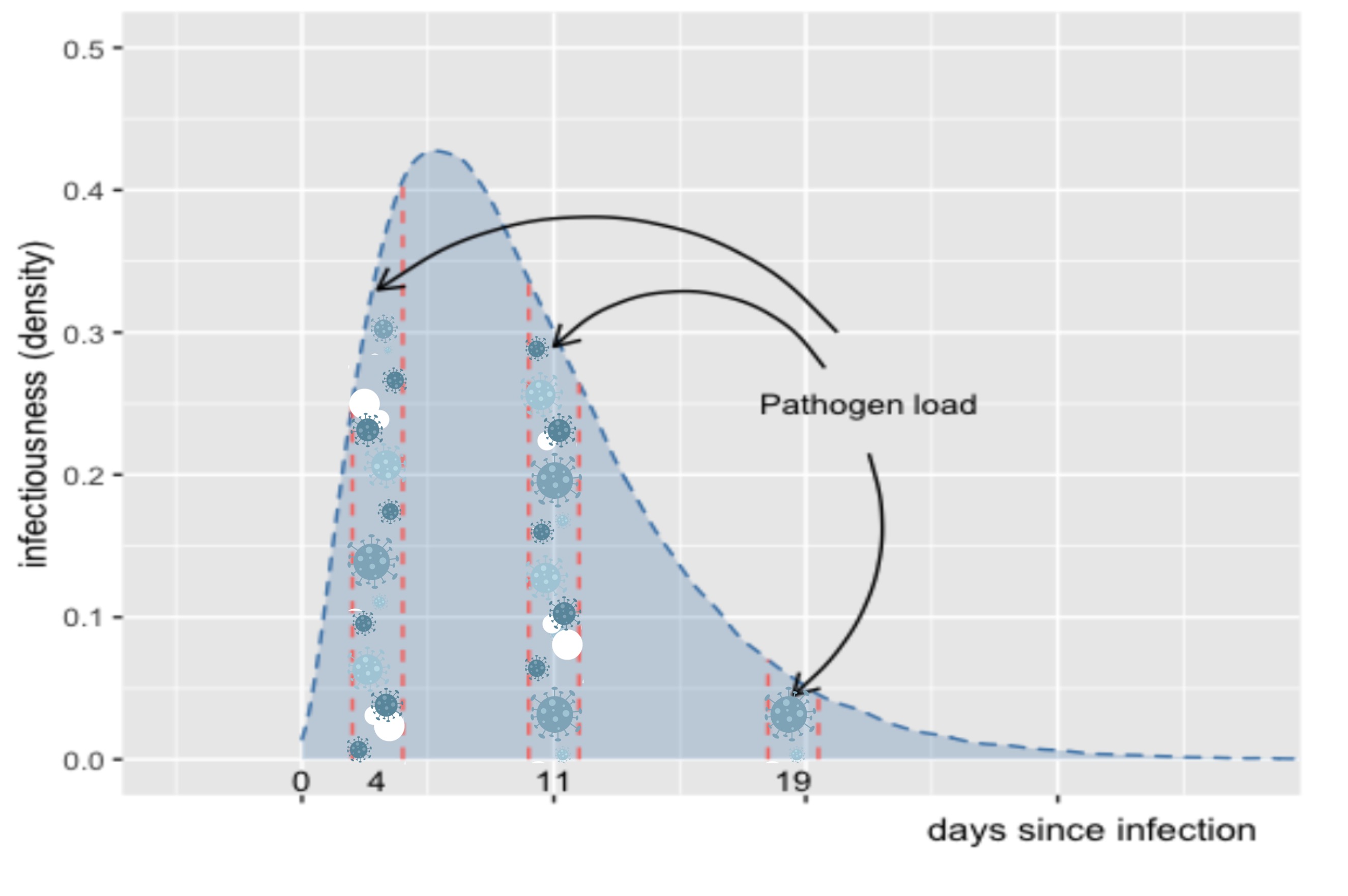
Figure 1: An example of the infectiousness function at day $s$ since infection, $\omega_{s}$, approximated using the density function of a gamma distribution with shape and rate parameters equals to 2.5 and 0.255 respectively. The above $\omega_{s}$ assumes that the infectiousness of an infected individual increases during the first 7 days since infection as viral loads increase soon after infection and then gradually decrease as the individual proceeds to recovery around 21 days after infection.

Based on these assumptions, we have $\mathbbm{E}(I_{t})=R_{t}\mathbbm{E}\int^{t}_{0}\omega_{s}I_{t-s}ds$. In practice, we can discretize time to be equally spaced time points, so

$$E(I_{t}|I_{0},\cdots,I_{t-1})=R_{t}\sum_{s=1}^{t}I_{t-s}\omega_{s}\triangleq R_{t}\Lambda_{t},$$ (2.1)

where $\sum_{s=0}^{\infty}\omega_{s}=1$. To estimate $R_{t}$ and $\omega_{s}$, it is natural to assume a distribution assumption for $I_{t}$ based on (2.1). For example, Cori et al. (2013) assumed a Poisson distribution, which is equivalent to model $\{I_{t},t\geq 0\}$ using a Poisson process. The model was used to study the epidemic of Ebola virus disease in west Africa (WHO Ebola Response Team, 2014). Recently, TSI model with an embedded regression structure is used to study COVID-19 (Quick et al., 2021).

3 The proposed Quasi-Score approach

Now, we introduce a quasi-score method based on the TSI model, which relaxes the distribution assumptions and allows estimation of covariates effects on disease transmission with the capability of accounting for errors in the data.

3.1 The proposed model

To relax distributional assumptions, we assume moment constraints on the number of incidence cases at time $t$ given observed incidence cases before time $t$ as follows.

$$\mu_{t} \triangleq\mathbbm{E}\big{(}I_{t}|\mathcal{F}_{t-1}\big{)}=\mathbbm{E}\big{(}R_{t}|\mathcal{F}_{t-1}\big{)}\Lambda_{t},\qquad\nu_{t}\triangleq\mbox{Var}\big{(}I_{t}|\mathcal{F}_{t-1}\big{)}=g(\mu_{t})\cdot\phi,$$ (3.1)

where $\phi$ is a dispersion parameter and $g(\cdot)$ is assumed to be a known variance function in the main manuscript. For a more general scenario where $g(\cdot)$ is unknown, we provide the estimation and discussion in the supplementary material. When $R_{t}\in\mathcal{F}_{t-1}$, $\mu_{t}=R_{t}\Lambda_{t}$. To estimate $R_{t}$, $t=1,\cdots,N$, and investigate the impacts of local area factors (or covariates), e.g., temperature, social distancing measures and population density, on disease transmission, we adopt a time series model such that

$$h(R_{t}) =X_{t}^{T}\beta+\sum_{i=1}^{q}\theta_{i}f_{i}(D_{1,t},D_{2,t},D_{3,t})+\epsilon_{t}.$$ (3.2)

where $X_{t}^{T}=(1,Z_{t}^{T})\in\mathcal{M}_{p\times 1}$ is the vector of intercept and covariates, $Z_{t}$, at time $t$ and $\theta_{i}\geq 0$ for $1\leq i\leq q$. Here $h(\cdot)$ and $f_{i}(\cdot)$ represent a known link function and functions of past data respectively, and

$$D_{1,t}=\big{\{}X_{j}\big{\}}_{0\leq j\leq t},\quad D_{2,t}=\big{\{}I_{j}\big{\}}_{0\leq j\leq t-1},\quad D_{3,t}=\big{\{}R_{j}\big{\}}_{0\leq j\leq t-1},\quad\mathcal{F}_{t-1}=\sigma(D_{1,t}\cup D_{2,t}).$$

The $\epsilon_{t}$ can be viewed as a measurement error term of $R_{t}$, although $R_{t}$ is not directly observed. Such an error can be due to errors in the observed data or model mis-specification. Alternatively, the $\epsilon_{t}$ can also be considered as a “random effect” for each day which captures the variation of $R_{t}$ that are not explained by the time series structure and the unobserved data in equation (3.2).

Therefore, the proposed model decomposes the serial dependency of incidence cases into two parts: equation (3.1) models the serial dependency that is due to the generative nature of disease transmission given $R_{t}$, and equation (3.2) models the serial dependency that is due to the dependency of $R_{t}$ between neighboring time points that can be explained by covariates and time series structures. Conceptually, the proposed model is similar to a recurrent neural network as shown in Figure 2.

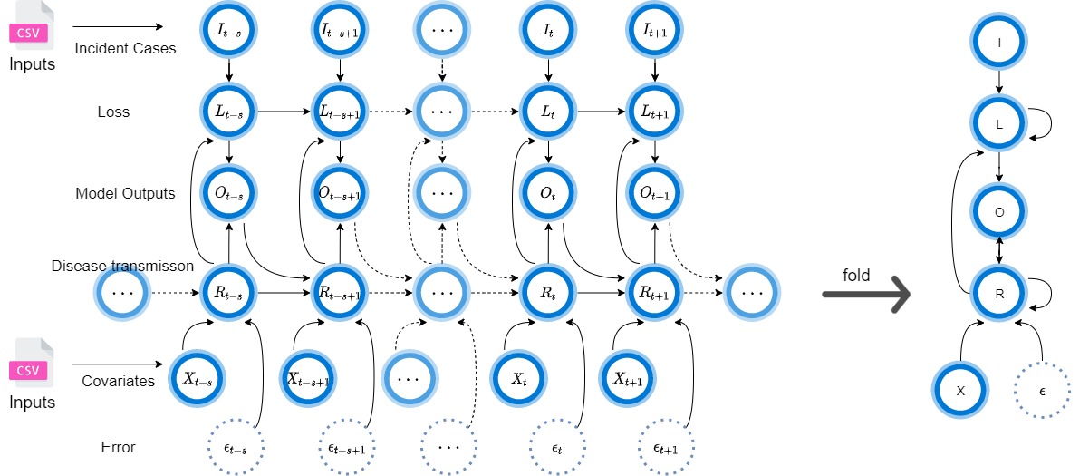
Figure 2: Workflow of the proposed dynamical systems described by model (3.1) and (3.2), illustrated as a recurrent neural network’s computational graph. Combine the information of incident cases ($I_{t}$) and daily covariates ($X_{t}$), the proposed model constructs and solves an estimating function which is similar to minimizing a loss function to estimate parameters, e.g., covariates effects, and the time series dependency of the instantaneous reproduction number ($R_{t}$).

In practice, a convenient special case of (3.2) is a non-stationary log-transmission model which assumes

$$\log(R_{t})=\phi_{0}+Z_{t}^{T}\beta+\sum_{i=1}^{q}\theta_{i}\log(R_{t-i})+\epsilon_{t},\quad{\rm for}\;\;t\geq q>0,\;\;\theta_{i}\geq 0,\;\;{\rm and}\;\|\theta\|_{1}<1$$ (3.3)

and $\mu_{t}=\nu_{t}$, where an $AR(q)$ model is used to model the time series dependency and the non-stationary of $R_{t}$ is due to the variation of exogenous covariates. We impose the regularity condition $\|\theta\|_{1}<1$ to ensure the causality of the time series when exogenous terms are bounded and known.

3.2 Estimation

The measurement error term in the proposed model, equation (3.2), improves the model robustness to model mis-specification and data errors, such as unobserved covariates for disease transmission and reporting errors in case data. However, it also brings difficulties in estimating $R_{t}$ and parameters.

When $\epsilon_{t}$ is assumed to be 0, equation (3.2) reduces to

$$h(R_{t}) =X_{t}^{T}\beta+\sum_{i=1}^{q}\theta_{i}f_{i}(D_{1,t},D_{2,t},D_{3,t}).$$ (3.4)

In this model, an estimator of the parameters $\gamma=(\beta,\theta)$, denoted as $\hat{\gamma}$, can be obtained by solving $U_{N}({\gamma})=0$, where $U_{N}(\gamma)$ is the quasi-score estimating function

$$U_{N}(\gamma)=\sum_{t=q}^{N}\big{(}\frac{\partial\mu_{t}}{\partial\gamma}\big{)}^{T}\nu_{t}^{-1}(I_{t}-\mu_{t})\triangleq\sum_{t=q}^{N}\xi_{t}(\gamma).$$ (3.5)

Here, we assume the infectiousness function $\omega=\{\omega_{s},1\leq s\leq\eta\}$ is known in most practical scenarios, e.g., He et al. (2020) for COVID-19 viral shedding, assuming that some prior knowledge about the pathogen transmission profile has been reported previously. In situations when estimates of $\omega$ are reported from multiple studies, we can conduct a meta-analysis to obtain a pooled estimate before plugging into equation (3.5). In cases when it is unknown, it can be estimated through (3.5) with a constraint $\sum_{s=1}^{\eta}\omega_{s}=1$ where $\eta$ is known. In the rest of the manuscript, we assume $\omega$ to be known unless otherwise stated.

When $\epsilon_{t}$ is a non-degenerate random variable, calculating the expectation in $\mu_{t}=\mathbbm{E}[R_{t}|\mathcal{F}_{t-1}]\Lambda_{t}$ and solving $U_{N}(\gamma)=0$ are difficult in general. Similar models were studied by Davis et al. (2003) to model counts data using log link function, where the measurement error was assumed to be a stationary process and calculated using autoregressive moving average recursion with a distributed lag structure.

However, since we don’t have direct observations ($R_{t}$) for the time series (3.2) in this hierarchical model, so we describe an iterative method tailored for estimating parameters of (3.2), without requiring stationary structure and distribution assumption on the measurement error. Briefly, the proposed iterative algorithm consists of two steps. The first step uses the second layer of the model, the time series model, to construct a semi-parametric locally efficient estimator of $\beta$ based on a location-shift regression model. In this step, $\beta$ and $R_{t}$ can be written as functions of $\theta$ using an initial estimates of $\theta$ or an estimate from the last iteration. In the second step, the parameters were updated using the first layer of the model, the quasi-score estimating function.

More specifically, we first rearrange the intercept term in $X_{t}^{T}=(1,Z_{t}^{T})$ into the autoregressive term. Then equation (3.2) can be rewritten as

$$h(R_{t})-\sum_{i=1}^{q}\theta_{i}f_{i}(D_{1,t},D_{2,t},D_{3,t})=Z_{t}^{T}\beta+\epsilon_{t},\quad t=1,\cdots,N.$$

Assuming the Gauss-Markov assumption (Wooldridge, 2016), i.e, the conditional independence of $\{\epsilon_{t}|X_{t},t\geq 1\}$, $\mathbbm{E}[\epsilon_{t}|X_{t}]=0$ and homoscedasticity, the above equation forms a location-shift regression model. Thus, given a $\theta$ value, a semi-parametric locally efficient estimator (Tsiatis, 2007) for $\beta$ is obtained by

$$\hat{\beta}=\left\{\sum_{t=1}^{N}(Z_{t}-\bar{Z})(Z_{t}-\bar{Z})^{T}\right\}^{-1}\sum_{t=1}^{N}(Z_{t}-\bar{Z})\left(h(R_{t})-\sum_{t=1}^{q}\theta_{i}f_{i}(D_{1,t},D_{2,t},D_{3,t})\right),$$ (3.6)

where $\bar{Z}=\big{(}\sum_{t=1}^{T}Z_{t}\big{)}/N$ and $N$ is the number of observations. Based on this formulation, we recommend an iterative method, namely the Quasi-score online estimation for infectious disease (QSOEID), to estimate $\gamma$ and $R_{t}$ by iteratively updating the locally-efficient semi-parametric estimator of $\beta$ and the quasi-score estimator of $\theta$ as shown in Algorithm 1. Intuitively, with an initial estimate of $\theta$, intermediate estimates of $\beta$ and $R_{t}$ can be written as functions of the initial estimate of $\theta$ using equations (3.6) and (3.1) respectively. Then $\theta$ can be further updated by solving equation (3.5). The algorithm is run iteratively until it converges.

Due to its iterative nature, this procedure provides an online estimator for $\{R_{t}\}_{1\leq t\leq N}$ and $\gamma$ that can be updated daily or when data of new time points are available. The obtained estimates can also be used to forecast future $\{R_{t}\}_{t>N}$ with projected covariates. Furthermore, these estimates and forecasts can be used to support policy-making by building a utility function to evaluate a set of interventions. For example, denote $\hat{I}_{t+m}$ and $\hat{R}_{t+m}$ as the forecasts from the proposed model, then for an intervention option $A$ that belongs to the set of interventions $\mathcal{S}$, we may seek

$${\rm Optimal\;prevention\;option}=\min_{A\in\mathcal{S}}\;\mu(A)$$

$${\rm where}\quad\mu(A)=\mu_{1}(\hat{I}_{t+m})+\mu_{2}({\rm Economy})+\mu_{3}({\rm Mental\;health})+\mu_{4}({\rm Hospital\;capacity})+$$

$$\mu_{5}\Big{(}\hat{R}_{t+m}\cdot\mathbbm{1}(\hat{R}_{t+m}\geq 1)+\mathbbm{1}(\hat{R}_{t+m}<1)\Big{)}.$$

Here $\mu_{1}\sim\mu_{5}$ are utility functions for different social considerations. When $\mu(A)\leq\mu(B)\Leftrightarrow A\preceq B$ it suggests $A$ is preferred over B.

Algorithm 1 : The QSOEID algorithm
Estimation of the instantaneous reproduction number and covariates effects

1:procedure  Initialize the parameters using data from a small initial period of the pandemic $\tau_{0}$ and the model (3.4) that ignores measurement error. Denote the initial values as $\hat{\theta}^{(\tau_{0})}$, $\hat{\beta}^{(\tau_{0})}$ and $\{\hat{R}_{t}^{(\tau_{0})}\}_{0<t\leq\tau_{0}}$.

2:    loop

3:         for $k>\tau_{0}$, and $k\leq N$, with estimates $\hat{\theta}^{(k-1)},\hat{\beta}^{(k-1)}$, and $\{\hat{R}_{t}^{(k-1)}\}_{0<t\leq k-1}$ obtained in last iteration, do

4:             write the approximations of $\beta$ and $\{R_{t}\}_{\tau_{0}+1\leq t\leq k}$ as a function of $\theta$ using equations $(\ref{sudoestimator})$ and (3.1), that is

$$\tilde{\beta}^{(k)} \triangleq\left\{\sum_{t=1}^{k-1}(Z_{t}-\bar{Z}_{k-1})(Z_{t}-\bar{Z}_{k-1})^{T}\right\}^{-1}$$

$$\qquad\times\sum_{t=1}^{(k-1)}(Z_{t}-\bar{Z}_{k-1})\Big{[}h(\hat{R}_{t}^{(k-1)})-\sum_{s=1}^{q}\theta_{s}f_{s}\big{(}D_{1,t},D_{2,t},\hat{D}_{3,t}^{(k-1)}\big{)}\Big{]}$$ (3.7)

$${\text{and }}\tilde{R}_{t}^{(k)} \triangleq h^{-1}\left(\sum_{s=1}^{q}\theta_{s}f_{s}(D_{1,t},D_{2,t},\hat{D}_{3,t}^{(k-1)})+Z_{t}^{T}\tilde{\beta}^{(k)}\right),$$ (3.8)

5:             Obtain $\hat{\theta}^{(k)}$ by solving the quasi-score equation

$$U_{k}(\theta)=\sum_{t=\tau_{0}+1}^{k}\big{(}\frac{\partial\tilde{\mu}_{t}^{(k)}}{\partial\theta}\big{)}^{T}\big{(}\tilde{\nu}_{t}^{(k)}\big{)}^{-1}(I_{t}-\tilde{\mu}_{t}^{(k)})$$ (3.9)

using iterative methods, e.g. Newton-Raphson and iteratively reweighted least squares, where $\tilde{\mu}_{t}^{(k)}=\tilde{\nu}_{t}^{(k)}\triangleq\tilde{R}_{t}^{(k)}\Lambda_{j}$.

6:             Obtain $\hat{\beta}^{(k)}$ and $\{\hat{R}_{t}^{(k)}\}_{1\leq t\leq k}$ by plugging $\hat{\theta}^{(k)}$ into (3.7) and (3.8) as follows

$$\hat{\beta}^{(k)} \triangleq\left\{\sum_{t=1}^{k-1}(Z_{t}-\bar{Z}_{k-1})(Z_{t}-\bar{Z}_{k-1})^{T}\right\}^{-1}$$

$$\qquad\times\sum_{t=1}^{k-1}(Z_{t}-\bar{Z}_{k-1})\Big{[}h(\hat{R}_{t}^{(k-1)})-\sum_{s=1}^{q}\hat{\theta}_{s}^{(k)}f_{s}\big{(}D_{1,t},D_{2,t},\hat{D}_{3,t}^{(k-1)}\big{)}\Big{]},$$ (3.10)

$${\text{ and }}\hat{R}_{t}^{(k)} \triangleq h^{-1}\left(\sum_{s=1}^{q}\hat{\theta}_{s}^{(k)}f_{s}(D_{1,t},D_{2,t},\hat{D}_{3,t}^{(k)})+Z_{t}^{T}\hat{\beta}^{(k)}\right).$$ (3.11)

7:         end for

8:    end loop

9:end procedure

10:

Remark 3.1

The procedure provides a forward-looking method to estimate $R_{t}$’s (Lipsitch et al., 2020), it can also be modified to provide backward-looking estimates as shown in section A of the supplementary material. In our simulation study, we found the back-looking estimator (supplementary materials A.1) performs similarly with much less computing time and less sensitivity to initial values. In practice, whether to use the forward-looking or the forward-looking method is a trade-off between accuracy and computational cost.

3.3 Uncertainty quantification

The block bootstrap method introduced by Hall (1985) and Künsch (1989) can be used to quantify the uncertainty of the proposed online estimator. Here we illustrate the calculation for $\beta$. Given the time series case counts and covariates, $\{(I_{t},Z_{t})\}_{1\leq t\leq N}$, where $Z_{t}$ is a $p$-dimensional vector of covariates at time $t$, we assume $\beta$ is estimable using a block of data as long as the length of the block exceeds $\ell$, i.e., we require $\left(\sum_{t\in\mathcal{S}}(Z_{t}-\bar{Z}_{\mathcal{S}})(Z_{t}-\bar{Z}_{\mathcal{S}})^{T}\right)^{-1}$ to be well defined for arbitrary set $\mathcal{S}\subset\{1,\cdots,N\}$ with $|\mathcal{S}|\geq\ell$.

Denote a block of data up to time $t$ with length $l$ as $\xi_{t}=\Big{(}\big{(}I_{t-\ell+1},Z_{t-\ell+1}\big{)},\cdots,\big{(}I_{t},Z_{t}\big{)}\Big{)}$ for $t=\ell,\cdots,N$. We adopt the suggested $\ell=O(N^{1/3})$ from Bühlmann and Künsch (1999) and independently resample $s$ blocks of data with replacement, for $s=O(\lfloor(N-p-\tau_{0})/\ell\rfloor)$ (Bühlmann, 2002) to obtain $s$ bootstrap samples $\xi_{t_{1}},\xi_{t_{2}},\ldots,\xi_{t_{s}}$. For the effect of $j$-th covariate, $\beta_{j}$, where $j=1,\cdots,p$, denote the estimator based on the $i$-th sample as $\hat{\beta}^{*}_{t_{i},j}$ and the estimator using the whole data as $\hat{\beta_{j}}$. One may use $\{\hat{\beta}^{*}_{t_{i},j}-\hat{\beta}_{j}:i=1,\cdots,s\}$ to approximate the empirical distribution of $(\hat{\beta}_{j}-\beta_{j})$ or use $\{\hat{\beta}^{*}_{t_{i},j}:i=1,\cdots,s\}$ as an approximation of the empirical distribution of $\hat{\beta}_{j}$. Thus the level $1-\alpha$ bootstrap confidence interval of $\beta_{j}$ based on the $s$ samples, $(L_{j,\alpha/2,s}^{*},U_{j,\alpha/2,s}^{*})$, can be constructed by

$$L_{j,\alpha/2,s}^{*} =2\hat{\beta}_{j}-\sup\left\{t:\frac{1}{s}\sum_{i=1}^{s}\mathbbm{1}(\hat{\beta}^{*}_{t_{i},j}\leq t)\leq 1-\frac{\alpha}{2}\right\},$$

$$U_{j,\alpha/2,s}^{*} =2\hat{\beta}_{j}-\inf\left\{t:\frac{1}{s}\sum_{i=1}^{s}\mathbbm{1}(\hat{\beta}^{*}_{t_{i},j}\leq t)\geq\frac{\alpha}{2}\right\},\;\;\text{or}$$ (3.12)

$$L_{j,\alpha/2,s}^{*} =\inf\left\{t:\frac{1}{s}\sum_{i=1}^{s}\mathbbm{1}(\hat{\beta}^{*}_{t_{i},j}\leq t)\geq\frac{\alpha}{2}\right\},\;\;U_{j,\alpha/2,s}^{*} =\sup\left\{t:\frac{1}{s}\sum_{i=1}^{s}\mathbbm{1}(\hat{\beta}^{*}_{t_{i},j}\leq t)\leq 1-\frac{\alpha}{2}\right\}.$$

The confidence band of $\{\hat{R}_{t}\}_{t\geq 0}$ can be obtained similarly using the empirical quantiles of $\{\hat{R}_{t_{i},t}^{*},1\leq i\leq s\}_{t\geq 0}$ calculated from the bootstrap estimators of model parameters.

4 Properties of the Estimator and Algorithm

4.1 Asymptotic properties

The proposed method is a general approach for different counting processes and is robust to mis-specification of distribution assumptions. When the measurement error is ignored, i.e. $\epsilon_{t}=0$, the Poisson process used in (Cori et al., 2013) is a special case of (3.1) with $\nu_{t}=\mu_{t}$. Since $U_{t}(\gamma)\in\mathcal{F}_{t}$ and $\partial\mu_{t}/\partial\gamma,\mu_{t},\nu_{t}\in\mathcal{F}_{t-1}$, then $\{(U_{s}(\gamma),\mathcal{F}_{s}),s\geq q\}$ is a mean zero martingale sequence, indicating that $U_{N}(\gamma)$ is an unbiased estimating function. Denote the oracle parameter value as $\gamma_{0}$ and according to theorem 3 of Kaufmann (1987), we have

Theorem 4.1

Under condition 1 described in section B of the supplementary material and on the non-extinction set defined in (B.1),

$$\Big{[}\sum_{t=q}^{N}\mbox{Cov}\big{(}\xi_{t}(\gamma_{0})|\mathcal{F}_{t-1}\big{)}\Big{]}^{1/2}(\hat{\gamma}-\gamma_{0})\overset{d}{\longrightarrow}\mathcal{N}(0,I).$$ (4.1)

In supplementary material section B, we also show a special case of (3.4), given by

$$\log(R_{t})=x_{t}^{T}\beta+\sum_{i=1}^{q}\theta_{i}\left[\log(R_{t-i})-x_{t-i}^{T}\beta\right],\quad{\rm for}\;\;t\geq q>0,\;\;\theta_{i}\geq 0,\;\;{\rm and}\;\|\theta\|_{1}<1,$$ (4.2)

satisfies (4.1) under a more traceable condition 2.

4.2 Bias correction and property of the estimation procedure

When the measurement error cannot be ignored, the proposed iterative algorithm consists of two major steps: one utilizes the semi-parametric locally efficient estimator to write $\beta$ and $R_{t}$ as a function of $\theta$ and the other updates the estimates by solving the score equation. However, the latter step is subject to estimation bias due to the bias of the score equation with the non-zero measurement error term from equation (3.2) (Cameron and Trivedi, 2013). Bias correction in the general case (3.2) is difficult, but it can be tackled in (3.3) by requiring $\mathbbm{E}\big{(}e^{\epsilon_{t}}|\mathcal{F}_{t-1}\big{)}=c_{0}$ for some constant $c_{0}$ (Zeger, 1988). Therefore, we can correct the bias by modifying the quasi-score equation (3.9) to an unbiased estimating equation as follows

$$U_{k}^{*}(\phi_{0},\theta)=\sum_{t=\tau_{0}+1}^{k}\big{(}\frac{\partial\tilde{\mu}_{t}^{(k)}}{\partial\theta}\big{)}^{T}\big{(}\tilde{\nu}_{t}^{(k)}\big{)}^{-1}(I_{t}/c_{0}-\tilde{\mu}_{t}^{(k)}).$$

In practice, $c_{0}$ can be treated as a nuisance parameter and estimated by solving the quasi-score equation. Moreover, under (3.3), solving the modified quasi-score equation (3.9) is equivalent to obtaining

$$\big{(}\hat{\phi}_{0}^{(k)},\hat{\theta}^{(k)}\big{)}=\arg\max_{\|\theta\|_{1}<1}\sum_{t=\tau_{0}+1}^{k}\Big{(}I_{t}\log\tilde{R}_{t}^{(k)}-\tilde{R}_{t}^{(k)}\Lambda_{t}\Big{)},$$ (4.3)

where $\big{(}\hat{\phi}_{0}^{(k)},\hat{\theta}^{(k)}\big{)}$ is the MLE based on conditional profile likelihood of Poisson counts. Therefore, the proposed online estimation procedure guarantees the following properties. Proof of the theorems is presented in section C of the supplementary material.

Theorem 4.2 (Concavity)

When $k>\tau_{0}$, to update estimates in each iteration, equivalently to solve equation (4.3), is a globally concave maximization problem.

Theorem 4.3 (Iteration Difference)

Given regularity condition 3 in the supplementary material and observed case counts and covariates up to time $N$, $\{(I_{t},Z_{t})\}_{1\leq t\leq N}$, for each $1\leq i\leq q$,

$$\big{|}\hat{\theta}_{i}^{(k)}-\hat{\theta}_{i}^{(k-1)}\big{|}=O\Big{(}\frac{1}{k-1}+\frac{I_{k}}{\big{(}\sum_{t=\tau_{0}+1}^{k-1}I_{n}\big{)}}\Big{)},$$

where $k\leq N$ is the indicator of iteration.

Theorem 4.3 demonstrates the bound of step-wise difference of the online estimator between iterations, which decreases as the number of observation time increases. The above form was obtained using the backward-looking algorithm. Results of the forward-looking algorithm, which shares a similar form, is shown in supplementary material. But, the estimator’s consistency remains an open question as discussed in Davis et al. (2003). The difficulty arise from the measurement error $\{\epsilon_{s}\}_{s\geq 1}$ and the disease case series dependency $\{\Lambda_{s\geq 1}\}$ in the model. However, both elements are essential in modeling the dynamics of disease transmission. The measurement error is a major issue in the disease counts and covariates data, and $\{\Lambda_{s\geq 1}\}$ is the key feature describing the dynamic of infection. Similar but simplified models, which do not model the measurement errors and $\{\Lambda_{s\geq 1}\}$ are built for different contexts, e.g. studies of economics or disease without case series dependency (Davis et al., 1999, 2000, 2003; Fokianos et al., 2009; Neumann et al., 2011; Doukhan, Fokianos and Li, 2012; Doukhan, Fokianos and Tjøstheim, 2012). Inspired by the derivation and discussion in Davis et al. (2003), we conjecture that conditions requiring stationary and uniformly ergodic of $\log(R_{t}\Lambda_{t})$ are needed to establish the consistency of estimators of model (3.3), although these conditions may be difficult to verify in practice.

5 Simulation Studies

This section describes the simulation studies we conducted to assess the performance of the proposed method, including the relative bias, coefficient of variation of the estimates, and the coverage probability of the Bootstrap confidence interval, with a focus on the estimation of covariates effect size that motivates the study. In addition, a comparison between the proposed model and basic SIR model is presented in the supplementary material.

5.1 Simulation settings

Throughout the simulation, we generated daily data of SARS-CoV-2 case counts and associated covariates, and fit the semi-parametric time series model (3.3) which assumed the $R_{t}$’s have AR(1) dependency and were associated with two covariates, i.e., $q=1$ and $p=2$. Each scenario was repeated for 1,000 times to calculate the evaluation statistics. The infectivity function was assumed to be known and generated from a gamma distribution to mimic the result in a previous epidemiological study of SARS-CoV-2 cases in Wuhan, China (Li et al., 2020).

Data were simulated under various scenarios, including settings for which the fitted models were correctly specified or mis-specified. For scenarios with correctly specified models (scenarios 1-7), data were generated using parameters $(\phi_{0},\theta_{1},\beta_{1},\beta_{2})=(.5,.7,-.02,-.125)$, where the simulated $\{R_{t},t\geq 1\}$ mimicked the trend of the $R_{t}$ reported in Pan, Liu, Wang, Guo, Hao, Wang, Huang, He, Yu, Lin et al. (2020). We varied days of observation $T$, initial incident cases $I_{0}$, and used different distributions of error terms $\{\epsilon_{t}\sim_{i.i.d}\epsilon,t=1,\cdots,T\}$ to generate data. For settings in which the model was mis-specified (scenarios 8-9), data were simulated assuming $R_{t}$’s followed AR(2) dependency (i.e., $q=2$) or three covariates (i.e., $p=3$). The two daily covariates were simulated independently to mimic the real data of temperature in Philadelphia and data of social distancing from daily cellular telephone movement, provided by Unacast (Unacast, 2021, July 1st), which measured the percent change in visits to nonessential businesses, e.g., restaurants and hair salons during March 1st and June 30th, 2020. Details of parameter values used in each scenario and the generating distribution of covariates data are shown in Section A.2 of the supplementary materials.

Table 1: Relative bias, bias and coefficient of variation of the estimators, calculated by $\sum_{i=1}^{N_{s}}(\hat{\theta}_{i}-\theta)/N_{s}\theta$, $\sum_{i=1}^{N_{s}}(\hat{\theta}_{i}-\theta)/N_{s}$ and $\{\sum_{i=1}^{N_{s}}[\hat{\theta}_{i}-(\sum_{i=1}^{N_{s}}\hat{\theta}_{i}/N_{s})]^{2}\}^{1/2}/(\sum_{i=1}^{N_{s}}\hat{\theta}_{i}/N_{s})$ with $N_{s}=1000$ replicates. $\hat{\theta}$ indicates the estimated value and $\theta$ is the true value.

relative bias (%)					empirical bias ($\times 10^{-2}$)				coefficient of variation $\hat{\sigma}/\hat{\mu}$
Scenario	$\phi_{0}$	$\theta_{1}$	$\beta_{1}$	$\beta_{2}$	$\phi_{0}$	$\theta_{1}$	$\beta_{1}$	$\beta_{2}$	$\phi_{0}$	$\theta_{1}$	$\beta_{1}$	$\beta_{2}$
1	-2.41	-1.42	-0.34	5.03	-1.20	-0.99	-0.01	0.63	0.27	0.11	0.36	0.36
2	-2.94	-1.51	-1.19	6.26	-1.47	-1.05	-0.02	0.78	0.37	0.10	0.55	0.38
3	-1.15	-0.78	-0.47	2.19	-0.57	-0.55	-0.01	0.27	0.24	0.10	0.27	0.29
4	-2.08	-3.57	-0.04	7.18	-1.04	-2.50	-0.00	0.90	0.37	0.14	0.69	0.64
5	-4.87	-1.85	-5.67	5.00	-2.44	-1.29	-0.11	0.63	0.39	0.13	0.98	0.60
6	-1.10	-4.16	-4.47	6.90	-0.55	-2.91	-0.09	0.86	0.39	0.13	0.43	0.48
7	-4.20	-1.43	-0.53	8.22	-2.10	-1.00	-0.01	1.03	0.28	0.11	0.37	0.36
8	-17.83	-0.72	4.06	9.64	-8.92	-0.51	0.14	1.20	0.31	0.12	0.31	0.42
9	$\diagup$	$\diagup$	-17.67	9.95	$\diagup$	$\diagup$	-3.53	1.24	$\diagup$	$\diagup$	0.27	0.27

5.2 Simulation results

Table 1 shows the bias and coefficient of variation of the estimators in each scenario. In scenarios $1-5$, both the bias and the coefficient of variation decreased as the sample size or initial case count $I_{0}$ increased. The proposed estimator still showed good performance with a relatively larger bias and variance when the error term’s variance was increased up to a magnitude that was smaller than the product of covariates and their corresponding effect sizes (scenarios 1 vs 6). When the error term had a heavier tail (scenario 7), the algorithm still had robust performance.

Two types of mis-specification (scenarios 8 and 9) were considered. In scenario 8, an important time-varying covariate was omitted from the model. Due to the correlation between generated covariates through time, this scenario is different from increasing the error term’s variance only. In both mis-specified cases, estimators $(\hat{\phi}_{0},\hat{\theta})$ were close to the corresponding partial correlation coefficient rather than the oracle value. Although the mis-specification caused an increasing in estimation bias but the algorithm still provides a relatively accurate estimator for correctly specified parts, with small bias and coefficient of variation (scenarios 1, 8 and 9). Most importantly, as illustrated in Figure 3 from a random replication of the simulation, the estimated $R_{t}$’s still captured the tendency of oracle $\{R_{t}\}_{t\geq 0}$ especially when the time-series’ sample size increases.

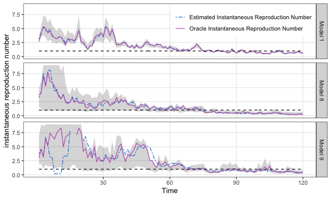
Figure 3: Estimated $R_{t}$’s and 90% bootstrap confidence bands from random replications of simulation, with block length $\ell=45$ and bootstrap replication $k=200$.

Table 2: Coverage Probability of $1-\alpha$ Empirical Bootstrap Confidence Interval for $\phi_{0}$

	T=300	T=300	T=300	T=450	T=450
	$\ell=30$	$\ell=45$	$\ell=60$	$\ell=30$	$\ell=45$
$\alpha=5\%$	96.4%	94.8%	93.0%	99.8%	99.2%
$\alpha=10\%$	91.2%	87.8%	86.2%	98.6%	97.2%
$\alpha=20\%$	83.4%	79.8%	77.2%	96.8%	93.2%

We also constructed the bootstrap confidence interval according to (3.12) and the coverage probability of bootstrap confidence interval for $\beta_{1}$ is shown in Table 2 as an illustration. Table 2 confirms that the proposed bootstrap confidence interval provides the expected coverage probability when chosen $\ell=45=\tau_{0}+O(T^{1/3})$ for $T=300$ following the recommendations in Bühlmann and Künsch (1999) and set the number of replications $k=500=O(T^{2/3})$ following Bühlmann (2002). When a smaller block length $\ell=30$ is chosen for $T=300$, the accuracy of the Bootstrap estimator is decreased compared to $\hat{\beta}_{1}$, leading to a conservative confidence interval. On the contrast, when a larger block length $\ell=60$ is chosen, despite the bootstrap estimator has better accuracy, the coverage probability is less than ideal due to high correlation between bootstrap subsample. Besides, the optimal block length also relates to $T$, as $\ell=30$ and $\ell=45$ would only results in a conservative confidence interval. Practically, we suggest to choose the smaller $\ell$ that satisfies $\ell=O(N^{1/3})$ from Bühlmann and Künsch (1999).

6 Application to COVID-19 Data

We applied the proposed method to a dataset which contained daily COVID-19 case count from 517 US counties representing 46 states and the District of Columbia between February 1st and July 6th 2020 and county level covariates, including demographics, social distancing measures and temperature variables. To be eligible, a county had to have $\varrho$ incident cases for more than two out of six consecutive days for at least 20 times (e.g., $\varrho=5$), as of June 1st, 2020 and meet at least one of the following criteria: 1) contained at least one city with population exceeding 100,000 persons; 2) contained a state capital; 3) the county was the most populated county in the state; or 4) average daily case incidence exceeded 20 during June 1st to June 30th, 2020. Within county, accumulative case count before the first $\varrho$ incidence cases was considered as $I_{0}$. As a sensitivity analysis, we explored three different $\varrho$ values, i.e. $\varrho=10,15$, and the analyses showed similar results so we presented the results with $\varrho=10$. The incidence threshold of 20 in 4) was selected based on empirical distribution of case counts in the observation time period. Daily incidence case count were smoothed using a 4-day moving average to reduce the impact of batch reporting. Our goals were to examine the association between county-level factors and $R_{t}$, to forecast the future case count, and to provide evidence for selecting appropriate social distancing policies.

6.1 Covariates selection and data preparation

We inherit three covariates described in an early study by Rubin et al. (2020): population density, social distancing and wet-bulb temperature. Social distancing is measured by a percent change in visits to nonessential businesses (e.g., restaurants, hair salons) revealed by daily cell-phone movement within each county, compared with visits in a four-week baseline period between February 10th and March 8th, 2020. Wet-bulb temperature is invoked since it has been demonstrated that humidity and temperature both play role in the seasonality of influenza. Further, a moving average with window length 11 days and a lag operator with delay of 3 days are imposed on the social distancing covariates and wet-bulb temperatures, based on the lag observed between change in social distancing and $R_{t}$ estimates and on an incubation period of at least 3 days. Other county-level covariates that we also considered includes demographic factors (e.g., age distribution, insurance status, etc), health-related factors (e.g., obesity, diabetes and proportion of individuals who smoke.), policy-related factors (e.g., mask wearing restrictions). Based on the correlation among the variables, we chose elderly population percentage from sociology related covariates and chose population percentage of diabetes from medical related covariates in the final model.

6.2 Covariates effect size estimation and interpretation

Table 3: Parameter estimates and bootstrap intervals from analyzing the county level COVID-19 data from 517 US counties between February 1st and July 6th 2020.

$\alpha$	$\varrho$	Elderly Pop.%,	Pop. Density	Diabetes %	Social Dist.	Wet-bulb Temp.
		$\beta_{1}$	$\beta_{2}$ ($\times 10^{-2}$)	$\beta_{3}$	$\beta_{4}$	$\beta_{5}$ ($\times 10^{-2}$)
0.05	10	2.438	2.001	6.666	0.608	-2.209
		(0.833, 5.633)	(-0.771, 5.373)	(1.848, 9.734)	(0.298, 1.624)	(-2.519, -0.485)
	15	2.660	3.695	7.159	0.726	-2.273
		(1.335, 5.624)	(1.639, 7.541)	(2.004, 11.43)	(0.576, 1.848)	(-2.625, -0.443)
$0.10$	$10$	(0.970, 5.154)	(-0.522, 4.944)	(2.006, 9.624)	(0.328, 1.404)	(-2.343, -0.539)
	$15$	(1.403, 5.542)	(1.745, 6.484)	(2.127, 11.19)	(0.633, 1.672)	(-2.537, -0.494)

• . For $\varrho=10$ and $15$, there are $444$ and $364$ counties and $38828$ and $30177$ observations, respectively. Bootstrap replication $k=200$ and block length $\ell=45$. Additional results from different $\varrho$ and $\ell$ values can be found in supplementary materials A.3.

The estimates and corresponding bootstrap intervals were demonstrated in Table 3. We found that, in addition to the strongest factor social distancing, population density, the percentage of elderly population and the percentage of diabetic population were also positively associated with $R_{t}$. It suggested that densely populated metropolitan counties with higher percentage of senior and diabetic population could have worse outbreaks comparing to rural counties with younger and healthier population. Note that temperature had negative impact on $R_{t}$, suggesting the transmission could slow down in warm weather. Although the effect size of temperature, $\hat{\beta}_{5}$, was small, its impact on policy making may be substantial, due to the wide range of temperature a county could experience within a year. During the study period, the largest increment of wet-bulb temperatures observed within a county was 32.8^∘C, which could reduce the transmission of COVID-19 by 51.5% with other covariates fixed. However, temperature could also affect social distancing values, as outdoor activities tended to increase during spring and summer, which could cancel out the reduction of transmission from increased temperature.

6.3 Estimating $R_{t}$ and forecasting future transmission

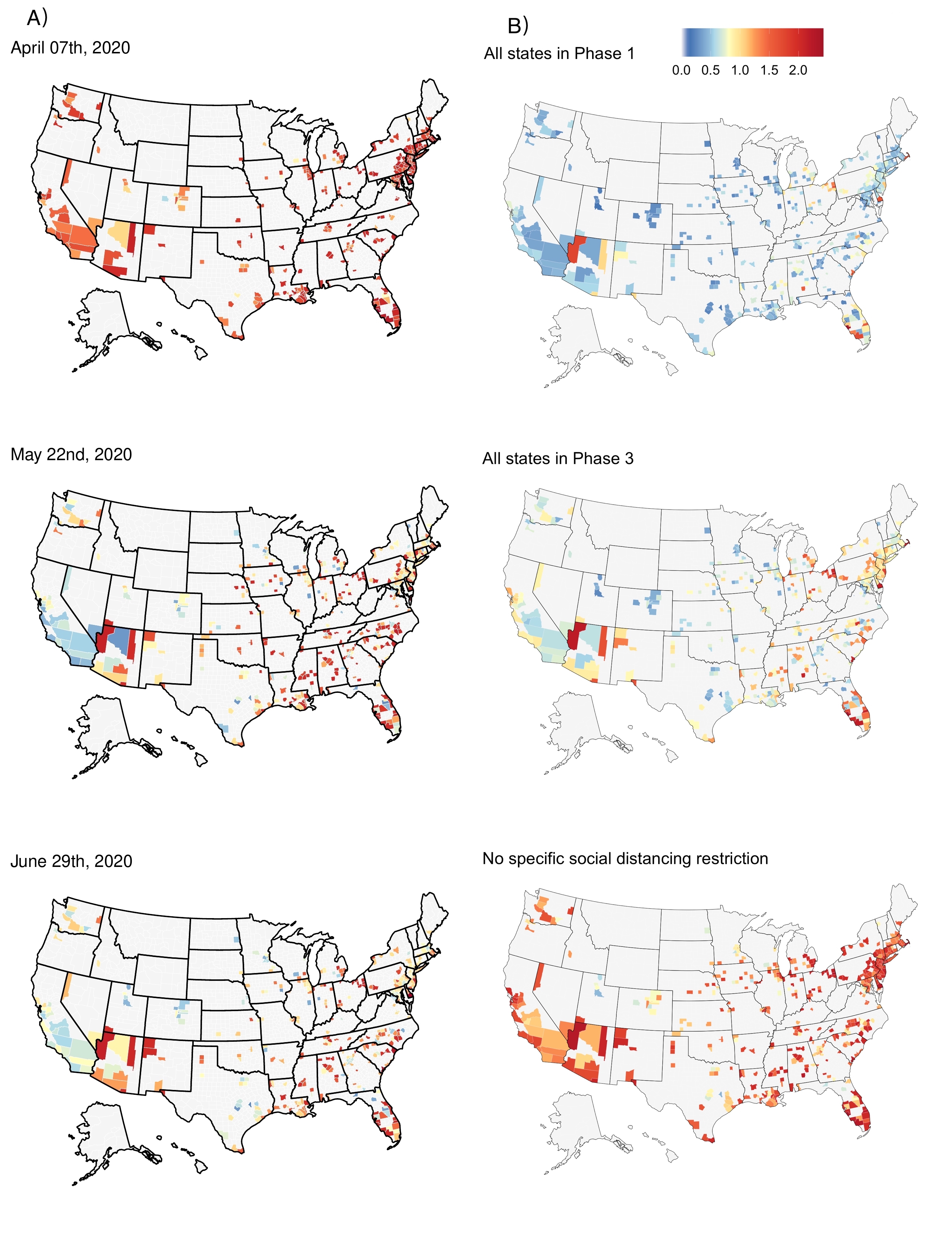
Figure 4: Heat maps for estimated and predicted county-level $R_{t}$ across United States. Roughly, $0<R_{t}<0.9$ : bluish, $0.9\leq R_{t}\leq 1.1$ : yellowish, $R_{t}>1.1$ : Reddish. Column A) shows estimated $R_{t}$ at three time points, which illustrates the shift of epicenter during April to June 2020. Column B) demonstrates predicted $R_{t}$ on September 1st based on three levels of social distancing

County-level $R_{t}$’s were estimated using the proposed QSOEID algorithm and backward estimation. The results clearly illustrated the evolution of the pandemic and the change of outbreak epicenter during the study period (Figure 4A). Due to space limit, we left more details on results interpretation and discussion to A.4 of supplementary materials. Based on the parameter estimates and projected values of covariates, we can forecast county-level disease transmission by calculating future $R_{t}$ and case count using the proposed model. In this application, we set social distancing value at three values, $-61.25\%$, $-35\%$ and $0\%$, to mimic the social distancing level under the reopening orders at Phase 1, Phase 3 and Phase 5 (without restriction), and used historical 10-year-average wet-bulb temperature to project the disease transmission. The three levels of social distancing were estimated by averaging data between May and June under different reopening orders. Taking the prediction at September 1st as an example, which is 57 days after the last day of the dataset. The predicted $R_{t}$ in Figure 4B presented the difference under different restrictions. These results can be used to support selection of intervention.

7 Discussion

In this paper, we proposed a novel model to predict and monitor disease transmission, evaluate covariates impact and investigate the generative nature of the virus. The time series dependency among the incidence case counts were decomposed into an epidemiological part, which was modeled using the TSI model, and a statistical part, which was modeled using an observed-driven model. We used the quasi-score method, together with an online algorithm, to estimate the instantaneous reproduction number and effects of covariates on disease transmission simultaneously. Our method contributed an exquisite gadget to a much larger toolbox in fighting the coronavirus pandemic.

Yet there are many feasible extensions of the model that are worth mentioning. Here we provide several hoping to inspire future discussion on possible improvements. First, the proposed method can be extended to a nonparametric model by relaxing the assumption on link function to avoid mis-specification (supplementary materials A.5). The estimation is straightforward if the dependency of $\{R_{t}\}_{t\geq 0}$ is ignored. When time series dependency of $\{R_{t}\}_{t\geq 0}$ is considered, e.g., $\mathbbm{E}\big{[}R_{t}|Z_{t},D_{3,t}\big{]}=\phi_{0}+\sum_{i=1}^{q}\theta_{i}f_{i}(R_{t-i})+g(Z_{t})$ with a known $R_{0}$ and known functions $f_{i}$, $1\leq i\leq q$ and unknown $g(\cdot)$, we can adopt local linear kernel estimators (Fan and Gijbels, 1996) into the proposed iterative algorithm. Second, the proposed method can be extended to model data from multiple regions using a random effect model (supplementary materials A.6) with an adapted distributional assumption on the random effect for individual region.

The proposed method also has a few limitations. First, heterogeneous testing capacity across the country and over time is a big challenge to the data quality. The errors due to testing capacity can be partially absorbed into the measurement error term in the proposed method, but without knowing the distribution of testing capacity (very likely changing over time), the proposed extension in supplementary materials A.6 may still fail to correct the bias rooted from these data errors. Another possible method to address this limitation is to use seroprevalence surveillance data to estimate the testing capacity, which will require the availability of additional data (Quick et al., 2021). Another limitation of the proposed method is related to the limitation of the TSI model, which uses only the incidence case data to estimate the instantaneous reproduction number. This leads to the fact that the performance of the proposed method could rely on the quality of case data. Although we proposed to use a measurement error term to address this challenge, it would be worthwhile to develop TSI models that can incorporate death or hospital admission data in future research.

References

- (1)
- Ardabili et al. (2020) Ardabili, S. F., Mosavi, A., Ghamisi, P., Ferdinand, F., Varkonyi-Koczy, A. R., Reuter, U., Rabczuk, T. and Atkinson, P. M. (2020), ‘Covid-19 outbreak prediction with machine learning’, Algorithms 13(10), 249.
- Boatto et al. (2018) Boatto, S., Bonnet, C., Cazelles, B. and Mazenc, F. (2018), ‘Sir model with time dependent infectivity parameter: approximating the epidemic attractor and the importance of the initial phase.’.
- Bühlmann (2002) Bühlmann, P. (2002), ‘Bootstraps for time series’, Statistical science pp. 52–72.
- Bühlmann and Künsch (1999) Bühlmann, P. and Künsch, H. R. (1999), ‘Block length selection in the bootstrap for time series’, Computational Statistics & Data Analysis 31(3), 295–310.
- Cameron and Trivedi (2013) Cameron, A. C. and Trivedi, P. K. (2013), Regression analysis of count data, Vol. 53, Cambridge university press.
- Cevik et al. (2021) Cevik, M., Tate, M., Lloyd, O., Maraolo, A. E., Schafers, J. and Ho, A. (2021), ‘Sars-cov-2, sars-cov, and mers-cov viral load dynamics, duration of viral shedding, and infectiousness: a systematic review and meta-analysis’, The lancet microbe 2(1), e13–e22.
- Chen et al. (2020) Chen, Y.-C., Lu, P.-E. and Chang, C.-S. (2020), ‘A time-dependent sir model for covid-19’, arXiv preprint arXiv:2003.00122 .
- Cori et al. (2013) Cori, A., Ferguson, N. M., Fraser, C. and Cauchemez, S. (2013), ‘A new framework and software to estimate time-varying reproduction numbers during epidemics’, American journal of epidemiology 178(9), 1505–1512.
- Costa-Santos et al. (2021) Costa-Santos, C., Neves, A. L., Correia, R., Santos, P., Monteiro-Soares, M., Freitas, A., Ribeiro-Vaz, I., Henriques, T. S., Rodrigues, P. P., Costa-Pereira, A. et al. (2021), ‘Covid-19 surveillance data quality issues: a national consecutive case series’, BMJ open 11(12), e047623.
- Davis et al. (2003) Davis, R. A., Dunsmuir, W. T. and Streett, S. B. (2003), ‘Observation-driven models for poisson counts’, Biometrika 90(4), 777–790.
- Davis et al. (1999) Davis, R. A., Dunsmuir, W. T. and Wang, Y. (1999), ‘Modeling time series of count data’, Statistics Textbooks and Monographs 158, 63–114.
- Davis et al. (2000) Davis, R. A., Dunsmuir, W. T. and Wang, Y. (2000), ‘On autocorrelation in a poisson regression model’, Biometrika 87(3), 491–505.
- Dayan et al. (2021) Dayan, I., Roth, H. R., Zhong, A., Harouni, A., Gentili, A., Abidin, A. Z., Liu, A., Costa, A. B., Wood, B. J., Tsai, C.-S. et al. (2021), ‘Federated learning for predicting clinical outcomes in patients with covid-19’, Nature medicine pp. 1–9.
- Doukhan, Fokianos and Li (2012) Doukhan, P., Fokianos, K. and Li, X. (2012), ‘On weak dependence conditions: the case of discrete valued processes’, Statistics & Probability Letters 82(11), 1941–1948.
- Doukhan, Fokianos and Tjøstheim (2012) Doukhan, P., Fokianos, K. and Tjøstheim, D. (2012), ‘On weak dependence conditions for poisson autoregressions’, Statistics & Probability Letters 82(5), 942–948.
- Fan and Gijbels (1996) Fan, J. and Gijbels, I. (1996), Local polynomial modelling and its applications: monographs on statistics and applied probability 66, Vol. 66, CRC Press.
- Fokianos et al. (2009) Fokianos, K., Rahbek, A. and Tjøstheim, D. (2009), ‘Poisson autoregression’, Journal of the American Statistical Association 104(488), 1430–1439.
- Fraser (2007) Fraser, C. (2007), ‘Estimating individual and household reproduction numbers in an emerging epidemic’, PloS one 2(8), e758.
- Hall (1985) Hall, P. (1985), ‘Resampling a coverage pattern’, Stochastic processes and their applications 20(2), 231–246.
- He et al. (2020) He, X., Lau, E. H., Wu, P., Deng, X., Wang, J., Hao, X., Lau, Y. C., Wong, J. Y., Guan, Y., Tan, X. et al. (2020), ‘Temporal dynamics in viral shedding and transmissibility of covid-19’, Nature medicine 26(5), 672–675.
- IHME COVID-19 forecasting team (2020) IHME COVID-19 forecasting team (2020), ‘Modeling covid-19 scenarios for the united states’, Nature medicine .
- Kaufmann (1987) Kaufmann, H. (1987), ‘Regression models for nonstationary categorical time series: asymptotic estimation theory’, The Annals of Statistics pp. 79–98.
- Kermack and McKendrick (1927) Kermack, W. O. and McKendrick, A. G. (1927), ‘A contribution to the mathematical theory of epidemics’, Proceedings of the royal society of london. Series A, Containing papers of a mathematical and physical character 115(772), 700–721.
- Künsch (1989) Künsch, H. R. (1989), ‘The jackknife and the bootstrap for general stationary observations’, Annals of Statistics 17(3), 1217–1241.
- Li et al. (2020) Li, Q., Guan, X., Wu, P., Wang, X., Zhou, L., Tong, Y., Ren, R., Leung, K. S., Lau, E. H., Wong, J. Y. et al. (2020), ‘Early transmission dynamics in wuhan, china, of novel coronavirus–infected pneumonia’, New England journal of medicine .
- Lipsitch et al. (2020) Lipsitch, M., Joshi, K. and Cobey, S. E. (2020), ‘Comment on pan a, liu l, wang c, et al.,” association of public health interventions with the epidemiology of the covid-19 outbreak in wuhan, china,” jama, published online april 10, 2020’.
- Neumann et al. (2011) Neumann, M. H. et al. (2011), ‘Absolute regularity and ergodicity of poisson count processes’, Bernoulli 17(4), 1268–1284.
- Pan, Liu, Wang, Guo, Hao, Wang, Huang, He, Yu, Lin et al. (2020) Pan, A., Liu, L., Wang, C., Guo, H., Hao, X., Wang, Q., Huang, J., He, N., Yu, H., Lin, X. et al. (2020), ‘Association of public health interventions with the epidemiology of the covid-19 outbreak in wuhan, china’, Jama 323(19), 1915–1923.
- Pan, Shen and Hu (2020) Pan, T., Shen, W. and Hu, G. (2020), ‘Spatial homogeneity learning for spatially correlated functional data with application to covid-19 growth rate curves’, arXiv preprint arXiv:2008.09227 .
- Punn et al. (2020) Punn, N. S., Sonbhadra, S. K. and Agarwal, S. (2020), ‘Covid-19 epidemic analysis using machine learning and deep learning algorithms’, MedRxiv .
- Quick et al. (2021) Quick, C., Dey, R. and Lin, X. (2021), ‘Regression models for understanding covid-19 epidemic dynamics with incomplete data’, Journal of the American Statistical Association 116(536), 1561–1577.
- Rubin et al. (2020) Rubin, D., Huang, J., Fisher, B. T., Gasparrini, A., Tam, V., Song, L., Wang, X., Kaufman, J., Fitzpatrick, K., Jain, A. et al. (2020), ‘Association of social distancing, population density, and temperature with the instantaneous reproduction number of sars-cov-2 in counties across the united states’, JAMA network open 3(7), e2016099–e2016099.
- Sáez et al. (2021) Sáez, C., Romero, N., Conejero, J. A. and García-Gómez, J. M. (2021), ‘Potential limitations in covid-19 machine learning due to data source variability: A case study in the ncov2019 dataset’, Journal of the American Medical Informatics Association 28(2), 360–364.
- Song et al. (2020) Song, P. X., Wang, L., Zhou, Y., He, J., Zhu, B., Wang, F., Tang, L. and Eisenberg, M. (2020), ‘An epidemiological forecast model and software assessing interventions on covid-19 epidemic in china’, MedRxiv .
- Tian et al. (2020) Tian, T., Tan, J., Jiang, Y., Wang, X. and Zhang, H. (2020), ‘Evaluate the risk of resumption of business for the states of new york, new jersey and connecticut via a pre-symptomatic and asymptomatic transmission model of covid-19’, Journal of Data Science p. 1.
- Tsiatis (2007) Tsiatis, A. (2007), Semiparametric theory and missing data, Springer Science & Business Media.
-
Unacast (2021, July 1st)
Unacast (2021, July 1st), ‘Social distancing
scoreboard’.
https://www.unacast.com/covid19/socialdistancing-scoreboard#methodology - Wallinga and Teunis (2004) Wallinga, J. and Teunis, P. (2004), ‘Different epidemic curves for severe acute respiratory syndrome reveal similar impacts of control measures’, American Journal of epidemiology 160(6), 509–516.
- Wang et al. (2020) Wang, L., Zhou, Y., He, J., Zhu, B., Wang, F., Tang, L., Kleinsasser, M., Barker, D., Eisenberg, M. C. and Song, P. X. (2020), ‘An epidemiological forecast model and software assessing interventions on the covid-19 epidemic in china’, Journal of Data Science 18(3), 409–432.
- WHO Ebola Response Team (2014) WHO Ebola Response Team (2014), ‘Ebola virus disease in west africa—the first 9 months of the epidemic and forward projections’, New England Journal of Medicine 371(16), 1481–1495.
- Wooldridge (2016) Wooldridge, J. M. (2016), Introductory econometrics: A modern approach, Nelson Education.
- Zeger (1988) Zeger, S. L. (1988), ‘A regression model for time series of counts’, Biometrika 75(4), 621–629.
- Zhou et al. (2020) Zhou, Y., Wang, L., Zhang, L., Shi, L., Yang, K., He, J., Zhao, B., Overton, W., Purkayastha, S. and Song, P. (2020), ‘A spatiotemporal epidemiological prediction model to inform county-level covid-19 risk in the united states’, Harvard Data Science Review .