A Note On The Canonical Formalism For Gravity

Abstract

We describe a simple gauge-fixing that leads to a construction of a quantum Hilbert space for quantum gravity in an asymptotically Anti de Sitter spacetime, valid to all orders of perturbation theory. The construction is motivated by a relationship of the phase space of gravity in asymptotically Anti de Sitter spacetime to a cotangent bundle. We describe what is known about this relationship and some extensions that might plausibly be true. A key fact is that, under certain conditions, the Einstein Hamiltonian constraint equation can be viewed as a way to gauge fix the group of conformal rescalings of the metric of a Cauchy hypersurface. An analog of the procedure that we follow for Anti de Sitter gravity leads to standard results for a Klein-Gordon particle.

1 Introduction

In this article, we will re-examine the canonical formalism for quantum gravity DeWitt , focusing on the case of an asymptotically Anti de Sitter (AAdS) spacetime $X$. One advantage of the AAdS case is that, because of holographic duality, it is possible to explain in a straightforward way what problem the canonical formalism is supposed to solve, thereby circumventing questions like what observables to consider and what is a good notion of “time.” In holographic duality, there is a straightforward notion of boundary time, and there is no difficulty in defining local boundary observables.

It is natural in holographic duality to study the matrix elements of a product of local boundary operators ${\mathcal{O}}_{\alpha}$ between given initial and final states. A typical example is $\langle\Psi|{\mathcal{O}}^{\prime}(t^{\prime},\vec{x}^{\prime}){\mathcal{O}}(t,\vec{x})|\chi\rangle$, with boundary insertions of local operators ${\mathcal{O}}^{\prime}$, ${\mathcal{O}}$ at points labeled by time $t$ and spatial coordinates $\vec{x}$, and with states $\chi$, $\Psi$ that are defined by initial and final conditions. For simplicity, in this article we restrict to $t^{\prime}>t$, to avoid having to discuss “timefolds.” In the canonical formalism of the boundary theory, one constructs for any Cauchy hypersurface $S_{\infty}$ in the boundary of $X$ a Hilbert space ${H}$ of quantum states with the property that if some set ${\mathcal{I}}$ labels a basis $|i\rangle$ of ${H}$, then an amplitude can be factored by inserting a sum over these states (fig. 1(a)):

$$\langle\Psi|{\mathcal{O}}^{\prime}(t^{\prime},\vec{x}^{\prime}){\mathcal{O}}(t,\vec{x})|\chi\rangle=\sum_{i\in{\mathcal{I}}}\langle\Psi|{\mathcal{O}}^{\prime}(t^{\prime},\vec{x}^{\prime})|i\rangle\langle i|{\mathcal{O}}(t,\vec{x})|\chi\rangle.$$ (1)

This factorization is most naturally described in path integrals if ${\mathcal{O}}$ is to the past of $S_{\infty}$ and ${\mathcal{O}}^{\prime}$ is to the future. Such factorization can be iterated; for example, given two boundary Cauchy hypersurfaces $S_{\infty}$ and $S^{\prime}_{\infty}$ with $S^{\prime}_{\infty}$ to the future of $S_{\infty}$, and insertions on the boundary arranged in time in a suitable way, one has (fig. 1(b))

$$\langle\Psi|{\mathcal{O}}^{\prime\prime}(t^{\prime\prime},\vec{x}^{\prime\prime}){\mathcal{O}}^{\prime}(t^{\prime},\vec{x}^{\prime}){\mathcal{O}}(t,\vec{x})|\chi\rangle=\sum_{j^{\prime}\in{\mathcal{I}}^{\prime},\,i\in{\mathcal{I}}}\langle\Psi|{\mathcal{O}}^{\prime\prime}(t^{\prime\prime},\vec{x}^{\prime\prime})|j^{\prime}\rangle\langle j^{\prime}|{\mathcal{O}}^{\prime}(t^{\prime},\vec{x}^{\prime})|i\rangle\langle i|{\mathcal{O}}(t,\vec{x})|\chi\rangle$$ (2)

where the states $|i\rangle$ are defined on $S_{\infty}$ and the states $|j^{\prime}\rangle$ are defined on $S^{\prime}_{\infty}$. In writing the formula this way, we allow for the use of different bases ${\mathcal{I}}$ on ${\mathcal{S}}_{\infty}$ and ${\mathcal{I}}^{\prime}$ on $S^{\prime}_{\infty}$. The initial and final states $\chi$ and $\Psi$ in these formulas are themselves Hilbert space states defined in the far past and the far future.

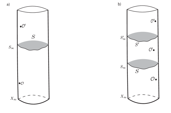
Figure 1: (a) The boundary $X_{\infty}$ of Anti de Sitter space, drawn as a cylinder, with boundary insertions ${\mathcal{O}}$ and ${\mathcal{O}}^{\prime}$ to the past and future of a Cauchy hypersurface $S_{\infty}\subset X_{\infty}$. In this setup, one can compute a matrix element $\langle\Psi|{\mathcal{O}}^{\prime}(t^{\prime},\vec{x}^{\prime}){\mathcal{O}}(t,\vec{x})|\chi\rangle$ as a sum over physical states defined on the hypersurface $S_{\infty}$. In the canonical formalism for gravity, one aims to find a similar formula in terms of a sum over states on a bulk Cauchy hypersurface $S$ with boundary $S_{\infty}$. (b) The “cutting” procedure of (a) can be iterated, with successive cuts on successive hypersurfaces.

The main result of the present article is a conceptually simple way to reproduce such factorization laws from a bulk point of view, to all orders of perturbation theory. The main idea is to exploit a relationship between Weyl invariance of a $(D-1)$-geometry and the Hamiltonian constraint equation of General Relativity.

Conformal approaches to quantization of gravity have a very long history York , and the conformal approach to the constraint equations, which gives particularly simple results in the case of an AAdS spacetime, has been much developed OY ; Ch ; CI ; I ; crusc ; BI . As we will see, the conformal approach is particularly powerful when it can be combined with existence and uniqueness results for maximal volume hypersurfaces, as was done for three-dimensional pure gravity in Monc ; KS ; BoS ; SK .

In section 2, we explain a bare minimum of this classical picture to motivate the approach that we will take to the canonical formalism of gravity. Then we go on to describe, by a simple gauge-fixing, a construction of a Hilbert space that is valid to all orders of perturbation theory. In section 3, we explain the underlying classical picture more thoroughly.

In early investigations of the canonical formalism for gravity DeWitt , it was observed that the Hamiltonian constraint of General Relativity is a family of second order differential operators, somewhat analogous to a Klein-Gordon operator. This suggested that the inner product for gravity might be defined by analogy with a Klein-Gordon bilinear pairing $(f,g)=\int_{S}{\mathrm{d}}\Sigma^{\mu}\overline{f}\overset{\leftrightarrow}{\partial_{\mu}}g$, which does not depend on the choice of the hypersurface $S$ on which it is evaluated. The analogy has always seemed problematical, because the Klein-Gordon pairing is not positive-definite, and also because the Hamiltonian constraint is a whole infinite family of second order operators, not just one. We will see that the procedure we follow for gravity, though it leads to a positive inner product, is closely analogous to a procedure which for a Klein-Gordon particle leads to the Klein-Gordon pairing.

Our analysis is restricted to perturbation theory for technical reasons, and it may be that this is inherent in assuming that ${H}$ can be constructed as a space of functions of fields – the metric tensor and possibly other fields – on a spacetime manifold. However, the result we get for the Klein-Gordon particle is exact, even though the derivation appears to be valid only in perturbation theory. In addition, the classical picture that motivates the present work is valid far beyond what is needed for perturbation theory. These facts suggest that in some admittedly unclear sense, the description of canonical quantization given in the present article might extend beyond perturbation theory. This possibility has motivated the writing of section 3 of the present article. Much of that section is an explanation of the conformal approach to the classical constraint equations, largely following the useful review article crusc .

An early version of this work, but without the gauge-fixing construction of section 2.4, was presented in a lecture at the Princeton Center for Theoretical Science WittenLecture .

As already noted, the main idea in this article is to exploit a relationship between the Hamiltonian constraint equation of gravity and the group of Weyl rescalings of a Cauchy hypersurface. Another and arguably much deeper relationship between the Hamiltonian constraint and Weyl invariance has been developed in recent years. The $T\overline{T}$ deformation is a deformation of a two-dimensional quantum field theory that is irrelevant in the renormalization group sense and for which no ultraviolet completion is understood but that nonetheless leads to unexpected exact results Zam ; ZamTwo ; Cardy . The Wheeler-DeWitt equation (or the Hamiltonian constraint equation) of three-dimensional gravity without matter fields can be interpreted in terms of the $T\overline{T}$ deformation of two-dimensional conformal field theory Verl . This striking insight has been refined and generalized to higher dimensions, where the $T\overline{T}$ deformation becomes a $T^{2}$ deformation KLM ; Taylor ; HKST ; Shyam ; ALS . More recently and remarkably, it has been extended to include matter fields AKW . In the present article, the $T^{2}$ deformation plays no role in the input, but in a sense we run into the $T^{2}$ deformation in the output, since the formula that we get for the Hilbert space inner product of a theory with gravity involves a sort of $T^{2}$-deformed ghost determinant.

The approach in the present article is limited to perturbation theory because we will use a gauge-fixing condition that is only valid perturbatively. The approach via the $T^{2}$ deformation is, at the present time, limited to perturbation theory because a nonperturbative completion of the $T^{2}$ deformation is not known. As already noted, a limitation to perturbation theory may well be unavoidable in any description based on fields in spacetime.

2 Path Integrals and Physical States

2.1 The Phase Space As A Cotangent Bundle

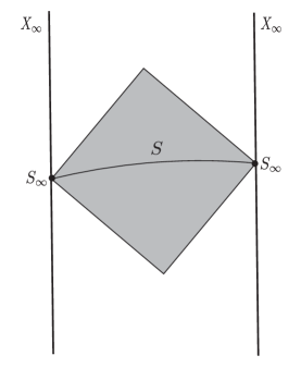
Figure 2: The bulk domain of dependence $\Omega$ of a Cauchy hypersurface $S_{\infty}$ in the boundary of an AAdS spacetime $X$. In this picture, for simplicity, $X$ is two-dimensional so its boundary $X_{\infty}$ is one-dimensional and $S_{\infty}$ consists of two points. $\Omega$ is the domain of dependence of any bulk Cauchy hypersurface $S$ with boundary $S_{\infty}$, or equivalently the set of bulk points that are not timelike separated from $S_{\infty}$.

We will defer a detailed discussion of the classical phase space of asymptotically Anti de Sitter (AAdS) gravity to section 3. Here we will explain a bare minimum to motivate an approach to the problem of describing a quantum Hilbert space.

The classical phase space of AAdS gravity is well understood in the case of pure gravity in three dimensions. Let $X$ be an AAdS three-manifold, globally hyperbolic in the AAdS sense, that satisfies Einstein’s equations with negative cosmological constant. Its conformal boundary $X_{\infty}$ consists of one or more copies of ${\mathbb{R}}\times S^{1}$ (where the ${\mathbb{R}}$ and $S^{1}$ directions are respectively timelike and spacelike). Let $S_{\infty}$ be any Cauchy hypersurface in $X_{\infty}$. There are many possible choices of bulk Cauchy hypersurface $S$ with boundary $S_{\infty}$, all homotopic to each other. The bulk domain of dependence of $S_{\infty}$, which we will call $\Omega$, can be defined as the domain of dependence of any $S$. An alternative definition of $\Omega$ which makes it obvious that $\Omega$ does not depend on the choice of $S$ is that $\Omega$ consists of points in $X$ that are not timelike separated from $S_{\infty}$ (fig. 2). Thus $\Omega$ is a pseudo-Riemannian manifold with boundary. $\Omega$ is the part of the spacetime that can be constructed, given initial data on $S$, just using Einstein’s equations, without using the AAdS boundary conditions along $X_{\infty}$.

By the phase space $\varPhi$ of AAdS gravity in this situation, we mean the space of possible geometries of the bulk domain of dependence $\Omega$, for a given choice of $S_{\infty}$. It is known (in the three-dimensional case) that $\varPhi$ is actually a cotangent bundle, $\varPhi=T^{*}({\sf{Conf}}/{\sf{Diff}})$, where ${\sf{Conf}}$ parametrizes conformal structures on $S$ (metrics modulo Weyl transformations $h\to e^{2\varphi}h$ with $\varphi|_{S_{\infty}}=0$) and ${\sf{Diff}}$ is the group of diffeomorphisms of $S$ that are trivial along $S_{\infty}$. Thus ${\sf{Conf}}/{\sf{Diff}}$ is the space of metrics on $S$ up to diffeomorphism and Weyl transformation. That $\varPhi=T^{*}({\sf{Conf}}/{\sf{Diff}})$ is proved as follows Monc ; KS ; BoS ; SK .

In one direction, one makes use of the renormalized volume of a hypersurface. In an AAdS spacetime, a Cauchy hypersurface $S$ has infinite volume, but it is possible to define a renormalized volume $V_{R}(S)$. In three dimensions, one shows that, for any given $S_{\infty}\subset X_{\infty}$ and any choice of the bulk spacetime $X$, there exists a unique bulk Cauchy hypersurface $S\subset X$ with boundary $S_{\infty}$ that maximizes $V_{R}(S)$. (See section 3.1 for a qualitative discussion of this existence and uniqueness.) $S$ has a Riemannian metric $h$ and a second fundamental form $K$; extremality of $V_{R}(S)$ implies that $K$ is traceless, ${\sf K}=0$ where ${\sf K}=h^{ij}K_{ij}$. Now, “forget” the metric $h$ and remember only the associated conformal structure, which we will call $h_{0}$ (thus, knowing $h_{0}$ means knowing $h$ up to a Weyl transformation $h\to e^{2\varphi}h$). Then $h_{0}$, up to diffeomorphism, defines a point in ${\sf{Conf}}/{\sf{Diff}}$. On the other hand, in General Relativity, $K$ is canonically conjugate to $h$. To be precise, the momentum conjugate to $h_{ij}$ is

$$\Pi^{ij}=\frac{1}{16\pi G}\sqrt{h}\left(K^{ij}-h^{ij}K^{r}_{r}\right).$$ (3)

The traceless part of this equation shows that the traceless part of $K$ is conjugate to the conformal structure $h_{0}$ (the trace ${\sf K}=K^{r}_{r}$ is conjugate to the volume density $\sqrt{\det h}$, which we abbreviate as $\sqrt{h}$). So the pair $K,h_{0}$, with $K$ being traceless, defines a point in $T^{*}{\sf{Conf}}$. To take diffeomorphisms into account, we have to divide by the group ${\sf{Diff}}$, but we also have to set to zero the Hamiltonian function on $T^{*}{\sf{Diff}}$ that generates the action of ${\sf{Diff}}$. Dividing by ${\sf{Diff}}$ removes from the phase space some modes of $h$ and setting the Hamiltonian function to zero removes the conjugate modes of $K$. For $K$ traceless, the Hamiltonian function that generates ${\sf{Diff}}$ is $D_{i}K^{ij}$. Setting the Hamiltonian function to zero is the momentum constraint of General Relativity. These matters are explained in sections 2.2 and 3.3. The combined operation of setting the Hamiltonian function to zero and dividing by ${\sf{Diff}}$ replaces $T^{*}{\sf{Conf}}$ with $T^{*}({\sf{Conf}}/{\sf{Diff}})$. So if $K$ and $h_{0}$ come from a solution of Einstein’s equations, they define a point in $T^{*}({\sf{Conf}}/{\sf{Diff}})$. The map that associates the pair $K,h_{0}$ to a given solution of the Einstein field equations therefore gives a map from the phase space $\varPhi$ to $T^{*}({\sf{Conf}}/{\sf{Diff}})$.

To get a map in the opposite direction, one shows that given a point in $T^{*}({\sf{Conf}}/{\sf{Diff}})$, that is, a pair $K,h_{0}$ with $D_{i}K^{ij}=0$, one can in a unique fashion make a Weyl transformation to a pair that satisfies the Einstein constraint equations and thereby gives initial conditions for a solution of the full Einstein equations, defining a point in $\varPhi$. The proof is explained in detail in section 3. The two maps are inverses, so the gravitational phase space can be identified as $\varPhi=T^{*}({\sf{Conf}}/{\sf{Diff}})$.

Are such ideas relevant to a general understanding of gravity? For this, something similar should be true in higher dimensions, and also in the presence of matter fields. The full story of what is known to be true and what is likely to be true under reasonable assumptions is somewhat involved, and is deferred to section 3. For now, we just remark that in the context of perturbation theory, in General Relativity on ${\mathrm{AdS}}_{D}$ or on ${\mathrm{AdS}}_{D}\times W$ for some compact manifold $W$, possibly with matter fields, an analysis similar to what was just sketched is always applicable. At least for purposes of perturbation theory, the phase space of such a theory can always be represented by a cotangent bundle $T^{*}{\sf Q}$, where now ${\sf Q}$ parametrizes the conformal structure of $S$ together with the matter fields on $S$, modulo diffeomorphisms that are trivial at infinity (along with gauge transformations that are trivial at infinity if some of the matter fields are gauge fields). That is true because both steps in the construction – existence of a unique $S$ of maximal volume, and existence of a unique Weyl transformation that ensures that the constraint equation is satisfied – are valid if one is sufficiently close to ${\mathrm{AdS}}_{D}$ or ${\mathrm{AdS}}_{D}\times W$. As we will discuss in section 3, to extend these results beyond perturbation theory, one requires a strong energy condition and a condition on singularities somewhat analogous to cosmic censorship. But such assumptions are not necessary in perturbation theory around ${\mathrm{AdS}}_{D}$ or ${\mathrm{AdS}}_{D}\times W$. Likewise, as we will also see in section 3, beyond perturbation theory one can make much stronger statements for ${\mathrm{AdS}}_{D}$ than for ${\mathrm{AdS}}_{D}\times W$, but the difference is not relevant in perturbation theory.

2.2 The Constraint Equations

The Einstein constraint equations are equations for a metric $h_{ij}$ on an initial value surface $S$ and a symmetric tensor field $K_{ij}$ on $S$. These equations are the condition under which $h$ and $K$ are initial data for a spacetime $X$ that satisfies Einstein’s equations, with $h$ (whose scalar curvature will be denoted $R(h)$) and $K$ understood as the induced metric and second fundamental form of $S\subset X$. For General Relativity with cosmological constant $\Lambda$ and no matter fields, the equations read

$${\mathcal{P}}^{j}({\vec{x}})={\mathcal{H}}({\vec{x}})=0,$$ (4)

with

$${\mathcal{P}}^{j}({\vec{x}}) =D_{i}K^{ij}-D^{j}K^{i}_{i}$$ (5)

$${\mathcal{H}}({\vec{x}}) =R(h)-K^{ij}K_{ij}+K^{i}_{i}K^{j}_{j}-2\Lambda.$$ (6)

The equation ${\mathcal{P}}^{j}({\vec{x}})=0$ is called the momentum constraint and the equation ${\mathcal{H}}({\vec{x}})=0$ is called the Hamiltonian constraint. Importantly, these are gauge constraints, which must be satisfied independently at each point ${\vec{x}}\in S$. Quantum mechanically, $K$ is conjugate to $h$ as in eqn. (3), so ${\mathcal{P}}^{j}({\vec{x}})$ and ${\mathcal{H}}({\vec{x}})$, for each ${\vec{x}}\in S$, become differential operators acting on the space ${\sf{Met}}$ of metrics on $S$. ${\mathcal{P}}^{i}({\vec{x}})$ is linear in $K$ so it becomes a first order differential operator which is simply the generator of diffeomorphisms of $S$; to be precise, if $v^{i}$ is a vector field on $S$ then the generator of the symmetry ${{\updelta}}x^{i}=v^{i}$ is $\int_{S}{\mathrm{d}}^{D-1}{\vec{x}}\sqrt{h}v^{i}({\vec{x}}){\mathcal{P}}_{i}({\vec{x}})$. ${\mathcal{H}}({\vec{x}})$ is quadratic in $K$, so it becomes a second order differential operator.

In the most basic version of the canonical approach to quantum gravity, the quantum wavefunction is a function $\Psi(h)$ of the metric of $S$ (and possibly other variables). The traditional interpretation of the constraint is that the operators obtained by quantizing the constraints should annihilate $\Psi(h)$:

$${\mathcal{P}}^{i}({\vec{x}})\Psi(h)={\mathcal{H}}(x)\Psi(h)=0.$$ (7)

Since ${\mathcal{P}}^{i}({\vec{x}})$ is the generator of diffeomorphisms, the constraint ${\mathcal{P}}^{i}({\vec{x}})\Psi=0$ merely says that $\Psi(h)$ should be invariant under diffeomorphisms of $S$ (or more precisely, under those diffeomorphisms that are connected to the identity; it is generally assumed that this condition should be extended to all diffeomorphisms). With this constraint imposed, $\Psi(h)$ becomes a function on the space ${\sf{Met}}/{\sf{Diff}}$ of metrics modulo diffeomorphisms. The Hamiltonian constraint ${\mathcal{H}}({\vec{x}})\Psi(h)=0$ is more vexing and more difficult to interpret. Because ${\mathcal{H}}({\vec{x}})$ is a second order differential operator for each ${\vec{x}}$, the constraint ${\mathcal{H}}({\vec{x}})\Psi(h)=0$ is an infinite system of second order differential equations that should be satisfied by the quantum wavefunction. This infinite system of equations (or sometimes the combined system ${\mathcal{P}}^{i}({\vec{x}})\Psi={\mathcal{H}}({\vec{x}})\Psi=0$) is known as the Wheeler-DeWitt equation. In the traditional approach to the canonical theory of gravity, a quantum wavefunction is a function on ${\sf{Met}}/{\sf{Diff}}$ that satisfies the Hamiltonian constraint equation, or equivalently a function on ${\sf{Met}}$ that satisfies the combined system ${\mathcal{P}}^{i}({\vec{x}})\Psi={\mathcal{H}}({\vec{x}})\Psi=0$.

A basic difficulty of canonical quantum gravity is that it is very difficult to solve the Wheeler-DeWitt equation, or to gain any qualitative understanding of the solutions. However, the fact that the phase space of General Relativity is a cotangent bundle $\varPhi=T^{*}({\sf{Conf}}/{\sf{Diff}})$ suggests a simple answer. In general, a cotangent bundle $T^{*}Y$ can be quantized by saying that a physical state is a square integrable function on the base space $Y$. So one is led to hope that the state space of General Relativity can be interpreted as a space of functions on ${\sf{Conf}}/{\sf{Diff}}$, with no constraints.

The original suggestion along these lines was actually made by York half a century ago York , for somewhat similar reasons to what was just explained, and motivated by even earlier results that pointed in this direction. For example, Kuchar had shown Kuchar that in asymptotically flat spacetime, to lowest nontrivial order, a solution $\Psi(h)$ of the Wheeler-DeWitt equation depends only on the transverse traceless part of $h$. To be precise, here we perturb around the case that $S$ is a flat hypersurface ${\mathbb{R}}^{D-1}$ in $D$-dimensional Minkowski space ${\mathbb{R}}^{D-1,1}$. The metric of $S$ is thus taken to be $h_{ij}=\delta_{ij}+h^{\prime}_{ij}$, where $\delta_{ij}$ is the Euclidean metric on ${\mathbb{R}}^{D-1}$ and $h^{\prime}_{ij}$ is the perturbation. Kuchar showed that to first order in $h^{\prime}$, the Wheeler-DeWitt equations assert that the quantum wavefunction $\Psi(h)$ is completely determined by an arbitrary function of the transverse traceless part of $h^{\prime}$. In lowest order, the space of transverse traceless metric perturbations is the same as the space of deformations of the conformal structure up to diffeomorphism, so Kuchar’s result can be restated by saying that to first non-trivial order, solutions of the Wheeler-DeWitt equation on ${\sf{Met}}/{\sf{Diff}}$ are in natural correspondence with functions on ${\sf{Conf}}/{\sf{Diff}}$. These arguments were recently reworked in the AAdS case, with a similar result CGPR .

The relation of the Wheeler-DeWitt equation to the $T\overline{T}$ deformation and its generalizations Verl ; KLM ; Taylor ; HKST ; Shyam ; ALS ; AKW actually gives a way to generalize such statements to all orders in perturbation theory. In explaining this, we will just consider the original example Verl of three-dimensional pure gravity with $\Lambda<0$ and the original $T\overline{T}$ deformation Zam ; ZamTwo ; Cardy . The Wheeler-DeWitt equation of three-dimensional pure gravity reads

$$\left(K^{ij}K_{ij}-K^{i}_{i}K^{j}_{j}-R(h)+2\Lambda\right)\Psi(h)=0.$$ (8)

Setting $\Lambda=-1/\ell^{2}$ and using eqn. (3) to express $K$ in terms of $\Pi^{ij}(x)=-{\mathrm{i}}\frac{\delta}{\delta h_{ij}(x)}$, the equation becomes

$$\left(\frac{(16\pi G)^{2}}{\det h}\left(\Pi^{ij}\Pi_{ij}-(\Pi^{k}_{k})^{2}\right)-R(h)-\frac{2}{\ell^{2}}\right)\Psi(h)=0.$$ (9)

Now conjugate the constraint operator by $\exp\left(\frac{1}{8\pi G\ell}\int_{S}{\mathrm{d}}^{2}x\sqrt{h}\right)$ or equivalently define

$$\Psi=\exp\left(\frac{1}{8\pi G\ell}\int_{S}{\mathrm{d}}^{2}x\sqrt{h}\right)\widehat{\Psi}.$$ (10)

The effect of this change of variables is to shift $\Pi^{ij}\to\Pi^{ij}-\frac{{\mathrm{i}}}{16\pi G\ell}\sqrt{h}h^{ij}$. The equation satisfied by the new wavefunction $\widehat{\Psi}$ is

$$\left(\frac{{\mathrm{i}}}{\sqrt{\det h}}\Pi^{k}_{k}+\frac{8\pi G\ell}{\det h}\left(\Pi^{ij}\Pi_{ij}-(\Pi^{k}_{k})^{2}\right)-\frac{\ell}{32\pi G}R(h)\right)\widehat{\Psi}=0.$$ (11)

The term $\frac{8\Pi G\ell}{\det h}\left(\Pi^{ij}\Pi_{ij}-(\Pi^{k}_{k})^{2}\right)$ is irrelevant in the renormalization group sense; by power counting, it is negligible at long distances. The leading long distance approximation to the equation is therefore simply

$$\left(\frac{{\mathrm{i}}}{\sqrt{\det h}}\Pi^{k}_{k}-\frac{\ell}{32\pi G}R(h)\right)\widehat{\Psi}(h)=0.$$ (12)

This equation is familiar in two-dimensional conformal field theory (CFT). The operator ${\mathrm{i}}\Pi^{k}_{k}$ is the generator of Weyl transformations of the metric, and so eqn. (12) describes violation of conformal invariance by the usual $c$-number anomaly proportional to $R(h)$. In fact, eqn. (12) is the usual anomalous Ward identity of a two-dimensional CFT with central charge

$$c=\frac{3\ell}{2G},$$ (13)

which is the Brown-Henneaux formula for the central charge of the boundary stress tensor in three-dimensional gravity BH . Eqn. (11) differs from the usual CFT Ward identity by the $\Pi^{2}$ terms. Since $\Pi^{ij}=-{\mathrm{i}}\frac{\delta}{\delta h_{ij}}$ inserts a factor of the stress tensor $T^{ij}$ in an amplitude of the boundary CFT, eqn. (11) actually describes the combined violation of conformal invariance by the CFT anomaly along with a $T\overline{T}$ deformation. This was the main observation in Verl . If we factor the metric $h$ as $h=e^{2\varphi}h_{0}$, with some fixed choice of $h_{0}$, then we get $\Pi^{i}_{i}=-\frac{{\mathrm{i}}}{2}\frac{\delta}{\delta\varphi}$ and eqn. (12) becomes the usual CFT Ward identity that determines the dependence of $\widehat{\Psi}$ on $\varphi$. In eqn. (11), the $\Pi^{2}$ terms are of relative order $e^{-2\varphi}$ compared to the other terms. So for large $\varphi$, eqn. (11) reduces to the usual CFT Ward identity (12). Any solution $\widehat{\Psi}_{0}$ of that CFT Ward identity can be promoted as follows to a solution $\widehat{\Psi}$ of the $T\overline{T}$-deformed equation (11). Let us denote the operators on the left hand sides of eqns. (11) and (12) as $\mathcal{D}$ and $\mathcal{D}_{0}$, respectively. We expand $\widehat{\Psi}=\widehat{\Psi}_{0}+\widehat{\Psi}_{1}+\widehat{\Psi}_{2}+\cdots,$ and stipulate that for large $\varphi$, each $\widehat{\Psi}_{k}$ is of order $e^{-2k\varphi}$ relative to $\widehat{\Psi}_{0}$ and that

$${\mathcal{D}}_{0}\widehat{\Psi}_{k}=-{\mathcal{D}}\left(\widehat{\Psi}_{0}+\widehat{\Psi}_{1}+\cdots+\widehat{\Psi}_{k-1}\right)+{\mathcal{O}}(e^{-2(k+1)\varphi}\Psi_{0}).$$ (14)

Order by order in $e^{-2\varphi}$, $\widehat{\Psi}_{k}$ is uniquely determined and eqn. (11) is satisfied. The expansion in powers of $e^{-2\varphi}$ is equivalently an expansion in powers of $G$. Thus, order by order in perturbation theory in $G$, $\widehat{\Psi}$ is uniquely determined in terms of $\widehat{\Psi}_{0}$. Every $\widehat{\Psi}$ arises in this way from some $\widehat{\Psi}_{0}$ (which can be found from the large $\varphi$ behavior of $\widehat{\Psi}$). Since the usual CFT Ward identity determines the dependence of $\widehat{\Psi}_{0}$ on $\varphi$, this means that order by order in perturbation theory, solutions $\widehat{\Psi}$ of the Wheeler-DeWitt equation are in natural correspondence with wavefunctions that depend on $h_{0}$ only, or in other words, functions on ${\sf{Conf}}/{\sf{Diff}}$. One can view this as a generalization of the result of Kuchar ; CGPR to all orders, in AAdS spacetime.

Knowing this correspondence does not immediate tell us the correct form of the Hilbert space inner product on the space of solutions of the Wheeler-DeWitt equation. One can formally define a natural inner product for functions on ${\sf{Conf}}/{\sf{Diff}}$ by $(\Psi^{\prime},\Psi)=\int_{{\sf{Conf}}/{\sf{Diff}}}\overline{\Psi}^{\prime}\Psi$. A more general inner product would be

$$\langle\Psi^{\prime},\Psi\rangle=(\Psi^{\prime}|\Xi|\Psi),$$ (15)

for some positive self-adjoint operator $\Xi$. In section 2.4, we will show how a simple gauge-fixing leads to a description of the perturbative Hilbert space ${H}$ of quantum gravity, roughly along these lines (but in a BRST formulation with ghost fields included), with a relatively simple and relatively explicit formula for $\Xi$ as a ghost determinant. The derivation will also lead directly to formulas such as eqns. (1) and (2), with transition amplitudes expressed in terms of sums over contributions of intermediate states in ${H}$. Such formulas are after all the goal of having a Hilbert space of physical states. However, first we will say more in section 2.3 about old and new approaches to the Wheeler-DeWitt equation and how the procedure in section 2.4 relates to them.

2.3 The Wheeler-DeWitt Equation And The BRST Operator

The traditional interpretation of the Wheeler-DeWitt equation, going back to its origins, was as described in section 2.2: a quantum state was taken to be a function $\Psi(h)$ of a $(D-1)$-geometry $h$, satisfying ${\mathcal{P}}^{i}(\vec{x})\Psi(h)={\mathcal{H}}(\vec{x})\Psi(h)=0$.

At least at a formal level, there is a specific problem in which a wavefunction of this type actually arises.

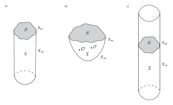
Figure 3: (a) Here $X_{\infty}$ is a Lorentz signature boundary manifold with a future boundary $S_{\infty}$. In the boundary theory, initial conditions in the far past, and possible boundary insertions, determine a quantum state $\Psi_{\infty}$ on $S_{\infty}$. The bulk is an AAdS manifold $X$ with future boundary $S$. The metric $h$ of $S$ is fixed and the path integral on $X$ defines a function $\Psi(h)$ which one hopes has the same physical content as $\Psi_{\infty}$. One can argue formally that $\Psi(h)$ satisfies the Wheeler-DeWitt equation. (b) A similar picture to (a) in Euclidean signature. The main difference is that $X_{\infty}$ has operator insertions but no past boundary. (c) The picture of (a) is continued into the future and some final state is specified. In the boundary one gets nice formulas for the transition amplitude between specified initial and final states involving a sum over states on $S_{\infty}$, but in bulk, there is a problem if the states are supposed to be solutions $\Psi(h)$ of the Wheeler-DeWitt equation. If one picks a particular bulk Cauchy hypersurface $S$ on which to cut, the Wheeler-DeWitt equation is not satisfied, but integrating over all $S$ gives a massive overcounting.

We consider some sort of initial conditions that, physically, should suffice to create a specific quantum state. For example, in the AAdS context, in Lorentz signature, we can do the following. From a boundary point of view (fig. 3(a)), we specify a Lorentz signature manifold $X_{\infty}$ of dimension $D-1$ that starts at time $t=-\infty$ in the past and has a spacelike future boundary $S_{\infty}$. The boundary theory on $X_{\infty}$, with initial condition at $t=-\infty$ corresponding to some chosen state, and specified operator insertions to the past of $S_{\infty}$, will produce a quantum state $\Psi_{\infty}$ on $S_{\infty}$. One can also make a similar construction in Euclidean signature (fig. 3(b)).

To recover the state $\Psi_{\infty}$ from the gravitational path integral, one considers a bulk spacetime $X$ with conformal boundary $X_{\infty}$ at spatial infinity, and terminating in the future on a spacelike hypersurface $S$ whose boundary is $S_{\infty}$. We write $g$ for the metric of $X$ and $h=g|_{S}$ for the induced metric on $S$. Now we do a bulk path integral, with initial conditions and boundary insertions as before, and with Dirichlet boundary conditions keeping fixed the metric $h$ of $S$. The output of the path integral is a function $\Psi(h)$. This function is supposed to define the state on $S$ created by the gravitational path integral under the given conditions.

The main virtue of this construction is that one can argue formally that $\Psi(h)$ satisfies the Wheeler-DeWitt equation. As the construction is manifestly invariant under diffeomorphisms of $S$, it is evident that ${\mathcal{P}}^{i}({\vec{x}})\Psi(h)=0$, and one can argue formally that ${\mathcal{H}}({\vec{x}})\Psi(h)=0$ (see for example HH ; Hall ; Barv ; Matz ). One can conjecture that $\Psi(h)$ is a bulk dual of the boundary state $\Psi_{\infty}$.

This construction has two drawbacks. The first is that the problem that was solved is not really the problem that one wanted to solve. The reason for wanting to construct a Hilbert space of quantum states is that one wants to be able to factorize transition amplitudes in terms of sums over intermediate states, as in eqns. (1) and (2). After all, this is what quantum states are good for in ordinary quantum mechanics. Although one can argue at a formal level that the wavefunction $\Psi(h)$ created by the gravitational path integral satisfies the Wheeler-DeWitt equation, there is no argument even formally that such wavefunctions participate in the desired “sum over states” formulas. The reason is that when we compute a path integral that we want to evaluate by summing over intermediate states, there is no natural way in the context of Dirichlet boundary conditions to find the bulk hypersurface $S$ whose metric $h$ we should be summing over (fig. 3(c)). General covariance would force us to integrate over all choices of $S$, which involves a massive overcounting.

The second drawback is that the gravitational path integral that is supposed to compute $\Psi(h)$ is actually not well-defined even in perturbation theory (and even after regularizing ultraviolet divergences), because the Dirichlet boundary condition that was assumed is not elliptic AE ; Anderson ; WittenBC . This lack of ellipticity means that, with Dirichlet boundary conditions, the operator $L$ that arises by linearizing the gauge-fixed Einstein equations about a classical solution does not have a well-defined determinant or propagator.

One might be inclined to dismiss the second problem as a technicality. However, if one actually tries to actually compute $\Psi(h)$ in perturbation theory in a specific situation, one will soon need the determinant and propagator of the operator $L$, and one will run into difficulties. There is actually another reason to believe that the non-ellipticity of the Dirichlet boundary condition on $L$ should not be dismissed lightly. This non-ellipticity can be straightforwardly proved, with a little linear algebra, starting from the definition of an elliptic boundary condition AE ; WittenBC . However, there is a more abstract proof that is quite instructive Anderson . In this proof, the only real input is the form of the Hamiltonian constraint equation for gravity and specifically the fact that it involves second derivatives of $h$ along the boundary (which appear in the scalar curvature $R(h)$) but only first derivatives in the normal direction to the boundary (which are present in the definition of ${\mathcal{H}}(\vec{x})$ in eqn. (5) because $K$ is linear in the normal derivative of $h$). The Hamiltonian constraint equation is the cause of the difficulty in understanding the canonical formalism for gravity, so in trying to understand that canonical formalism, we probably should not ignore a mathematical problem associated to the form of the constraint equation.

The problem involving the lack of ellipticity has a simple fix. Instead of Dirichlet boundary conditions for gravity in which one fixes the boundary metric, one can consider a mixed Dirichlet-Neumann boundary condition in which one specifies not the boundary metric $h$, but rather the conformal structure $h_{0}$ of the boundary (in other words, the boundary metric up to a Weyl transformation) and the trace ${\sf K}=K^{i}_{i}$ of the second fundamental form $K_{ij}$. This mixed Dirichlet-Neumann boundary condition is elliptic Anderson ; WittenBC , so in the situation of fig. 3(a), it should be possible in perturbation theory, after regularizing ultraviolet divergences, to use this boundary condition to compute a wavefunction $\Psi(h_{0},{\sf K})$.

One drawback of this is that the Wheeler-DeWitt equation in a dual version with ${\sf K}$ treated as a coordinate and $\sqrt{h}$ as a conjugate momentum appears to be, at best, no simpler than the original. Another and possibly more serious problem is that, again, this construction seems to solve the wrong problem. It formally gives a way to solve the problem described in fig. 3(a), but the problem of fig. 3(c) remains. There is no argument even formally that a gravitational path integral can be evaluated by “cutting” on an intermediate hypersurface $S$ and summing over states on $S$ of the form $\Psi(h_{0},{\sf K})$ that satisfy the constraint equations.

There is, however, also a standard fix for this difficulty. So far we have described what might be called the “traditional” Wheeler-DeWitt formalism. There is also a “revised” Wheeler-DeWitt formalism in which one constructs states that are better candidates for appearing in a factorization formula Nacht ; Higuchi ; Asht ; MarolfOther ; Embacher ; GM ; Marolf (see AKW and Appendix B of CLPW for recent discussions). In the revised Wheeler-DeWitt formalism, sometimes called refined algebraic quantization or group averaging, one still considers a wavefunction $\Psi(h)$, and one still imposes the momentum constraint equation ${\mathcal{P}}^{i}\Psi(h)=0$. However, the constraint ${\mathcal{H}}\Psi=0$ is replaced by an equivalence relation

$$\Psi(h)\cong\Psi(h)+\sum_{i}{\mathcal{H}}({\vec{x}}_{i})\chi_{i}(h)$$ (16)

for an arbitrary set of points ${\vec{x}}_{i}\in S$ and arbitrary functions $\chi_{i}(h)$. (The discrete sum over points ${\vec{x}}_{i}\in S$ can also be replaced by a continuous integral.) In other words, the sense in which ${\mathcal{H}}({\vec{x}})$ vanishes is not that it annihilates a physical state, but that its action is trivial, since any state ${\mathcal{H}}({\vec{x}})\chi$ is considered trivial. In this approach, any state $\Psi(h)$ that satisfies the momentum constraint is considered physical; two such states are considered equivalent if their difference is of the form $\sum_{i}{\mathcal{H}}({\vec{x}}_{i})\chi_{i}(h)$.

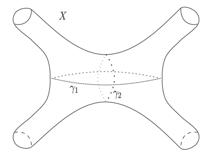
Figure 4: An AAdS spacetime $X$ with four asymptotic regions in which asymptotic states might be specified. Such an $X$ cannot have a metric everywhere of Lorentz signature; it may have Euclidean signature or possibly a complex metric. Overlapping “cuts” of such an $X$ can be made, as sketched here, on homotopically inequivalent surfaces such as $\gamma_{1}$ and $\gamma_{2}$. No one canonical formalism is well adapted to all of the possible cuts.

In this revised Wheeler-DeWitt approach, the inner product of two states is defined formally as

$$\langle\Psi^{\prime}|\Psi\rangle=\int_{{\sf{Met}}/{\sf{Diff}}}Dh\,\,\overline{\Psi}^{\prime}(h)\prod_{{\vec{x}}\in S}\delta({\mathcal{H}}({\vec{x}}))\Psi(h).$$ (17)

Here $Dh$ represents formally an integral over the space ${\sf{Met}}/{\sf{Diff}}$ of metrics on $S$ up to diffeomorphism. The product of delta functions $\prod_{{\vec{x}}\in S}\delta({\mathcal{H}}({\vec{x}}))$ formally annihilates any state of the form ${\mathcal{H}}({\vec{x}})\chi$, ensuring invariance of the inner product under the equivalence relation.

With this revised interpretation of the constraint operators, it is possible to give a formal argument that leads to the desired formulas involving cutting and summing over intermediate states, as in eqn. (1). For this, one goes to a canonical ADM formulation of the path integral in the region in which cutting is supposed to happen. In that formulation, the action contains a term $\int_{S}{\mathrm{d}}^{D-1}{\vec{x}}\,\,N({\vec{x}}){\mathcal{H}}({\vec{x}})$, where $N$ is called the lapse and does not appear elsewhere in the action. The path integral therefore contains a factor

$$\int DN\exp\left({\mathrm{i}}\int_{S}{\mathrm{d}}^{D-1}{\vec{x}}\,N({\vec{x}}){\mathcal{H}}({\vec{x}})\right).$$ (18)

Assuming that $N({\vec{x}})$ is supposed to be integrated from $-\infty$ to $+\infty$, the integral over $N$ gives formally the desired $\prod_{{\vec{x}}}\delta({\mathcal{H}}({\vec{x}}))$.

A possible criticism of this approach – the status of this issue is not clear to the author – is that in replacing the covariant version of the Einstein path integral with a canonical version in which $N$ is allowed to have either sign, we may have changed the path integral in a way that was adapted to the specific cutting formula we were trying to get. In the covariant path integral (or classically), it looks natural for $N$ to be positive. We really want to know how to evaluate the original covariant form of the path integral by a cutting formula. This issue is particularly sharp in a Euclidean signature context in which the boundary theory may satisfy many different formulas that result from cutting on topologically inequivalent hypersurfaces (fig. 4). No one canonical version of the bulk path integral can reproduce all of those different cutting formulas, so if one is going to use canonical versions of the path integral to deduce cutting formulas, it is essential to know that these canonical versions are all equivalent to the underlying covariant version of the path integral.

The traditional and revised Wheeler-DeWitt theories can be viewed as two special cases of what one can do with BRST quantization. In BRST quantization, one introduces ghost fields, of ghost number 1, that transform like the generators of the gauge symmetries, but with opposite statistics. In the case of gravity, the ghost fields are an anticommuting vector field $c^{\mu}(\vec{x},t)$. One also introduces additional multiplets consisting of antighost fields and auxiliary fields; this part of the construction is nonuniversal and depends on what gauge condition one wishes to impose. The BRST operator, in the context of gravity, is Frad

$$Q=\int_{S}{\mathrm{d}}^{D-1}\vec{x}\sqrt{h}\left(c^{0}(\vec{x}){\mathcal{H}}(\vec{x})+c^{i}(\vec{x}){\mathcal{P}}_{i}(\vec{x})+\cdots\right),$$ (19)

where the omitted terms do not affect the following remarks. This operator obeys $Q^{2}=0$, so one can define its cohomology. As usual, the cohomology of $Q$ is defined to consist of states $\Psi$ that satisfy $Q\Psi=0$, modulo the equivalence $\Psi\cong\Psi+Q\chi$ for any $\chi$. In BRST quantization, the cohomology at one particular (theory-dependent) value of the ghost number is defined as the Hilbert space of physical states. In the case of gravity, if we assume that we are interested in states that are not annihilated by any modes of $c^{0}$ and $c^{i}$ (and that therefore are annihilated by all modes of the conjugate antighosts), the condition $Q\Psi=0$ gives ${\mathcal{H}}({\vec{x}})\Psi={\mathcal{P}}_{i}({\vec{x}})\Psi=0$, the traditional Wheeler-DeWitt constraints. On the other hand, we could assume that we are interested in states that are annihilated by all modes of $c^{0}$ but not by any modes of $c^{i}$. Then the condition $Q\Psi=0$ gives the momentum constraint ${\mathcal{P}}_{i}(\vec{x})\Psi=0$, but not the Hamiltonian constraint ${\mathcal{H}}(\vec{x})\Psi=0$. Instead, the equivalence $\Psi\cong\Psi+Q\chi$ leads to the equivalence relation (17) of the revised Wheeler-DeWitt approach.

Thus the traditional and revised Wheeler-DeWitt theories are special cases of what one can do in the BRST framework. Neither of these corresponds closely to the way that BRST quantization is usually carried out in ordinary gauge theory or in perturbative string theory. Usually, the starting point is a relatively standard Fock space of ghost and antighost fields, with a basis of states that are annihilated by roughly half of the ghost modes and half of the antighost modes. In other words, in setting up the BRST machinery and using it to define the physical Hilbert space, ghosts and antighosts are usually treated rather similarly to other fields.

In the next section, we will describe a simple gauge-fixing that can be used to construct a Hilbert space for gravity. The construction is valid to all orders of perturbation theory, but not beyond, at least not in the present formulation. A factorization formula is manifest. The states that appear in the factorization formula are functions on ${\sf{Conf}}/{\sf{Diff}}$, the answer that is suggested by the relation of the gravitational phase space to $T^{*}({\sf{Conf}}/{\sf{Diff}})$. The boundary condition that is used in defining these states is the elliptic Dirichlet-Neumann boundary condition. The BRST approach to quantization is used, but not in the way that leads to either the traditional or the revised Wheeler-DeWitt theory. A fairly explicit formula for the inner product will emerge.

2.4 A Simple Gauge-Fixing To Construct A Perturbative Hilbert Space

The part of the BRST formalism for gravity that is universal involves the metric tensor $g_{\mu\nu}$ and the ghost field $c^{\mu}$. They transform as

$${{\updelta}}g_{\mu\nu}=D_{\mu}c_{\nu}+D_{\nu}c_{\mu},~{}~{}~{}{{\updelta}}c^{\mu}=c^{\alpha}\partial_{\alpha}c^{\mu},$$ (20)

where ${{\updelta}}$ represents the infinitesimal deformation generated by the BRST charge $Q$. These formulas satisfy ${{\updelta}}^{2}=0$, which corresponds to $Q^{2}=0$; since ${{\updelta}}^{2}=0$, any expression of the general form ${{\updelta}}\Lambda$ is BRST-invariant, for any $\Lambda$.

The rest of the BRST formalism depends on what gauge-fixing condition one wishes to impose. In general the desired gauge condition may be defined by a family of equations

$$P_{\Upsilon}(g)=0,$$ (21)

where we do not specify the nature of the labels $\Upsilon$ carried by these equations. (More generally, the $P_{\Upsilon}$ could depend on matter fields as well as on the metric.) To impose such a gauge condition, we add a family of antighost fields $\overline{c}_{\Upsilon}$ and auxiliary fields $\phi_{\Upsilon}$ with

$${{\updelta}}\overline{c}_{\Upsilon}=\phi_{\Upsilon},~{}~{}~{}{{\updelta}}\phi_{\Upsilon}=0,$$ (22)

consistent with ${{\updelta}}^{2}=0$. A simple way to implement a gauge-fixing that will impose the condition $P_{\Upsilon}(g)=0$ is to add to the action a gauge-fixing term

$$I_{\mathrm{gf}} ={{\updelta}}\left(\sum_{\Upsilon}\overline{c}_{\Upsilon}P_{\Upsilon}\right)=\sum_{\Upsilon}\left(\phi_{\Upsilon}P_{\Upsilon}-\overline{c}_{\Upsilon}{{\updelta}}P_{\Upsilon}\right)$$ (23)

$$=\sum_{\Upsilon}\left(\phi_{\Upsilon}P_{\Upsilon}-\overline{c}_{\Upsilon}\int_{X}{\mathrm{d}}^{D}x\frac{{{\updelta}}P_{\Upsilon}}{{{\updelta}}g_{\mu\nu}(x)}(D_{\mu}c_{\nu}(x)+D_{\nu}c_{\mu}(x))\right).$$ (24)

Thus, if we add to the action no other terms that involve $\phi_{\Upsilon}$, then $\phi_{\Upsilon}$ will behave as a Lagrange multiplier, imposing a gauge condition $P_{\Upsilon}=0$.

This procedure can be used to impose quantum mechanically any gauge condition that would be correct classically. A gauge condition is correct classically if on the diffeomorphism orbit of $g_{\mu\nu}$, there is a unique representative with $P_{\Upsilon}=0$. In practice, one usually has to content oneself with a gauge condition that is correct classically in the context of perturbation theory – in other words, a gauge condition that is correct on gauge orbits that are sufficiently close to some starting point. For topological reasons, it is usually not possible to find a gauge condition that is uniformly valid on all gauge orbits.

In the case of gravity, assuming that one is constructing perturbation theory in an expansion around a classical solution $g_{0}$ of Einstein’s equations, one can write the full metric as $g=g_{0}+g_{1}$, and impose a gauge condition on the perturbation $g_{1}$. A simple and convenient gauge condition (which goes by names such as harmonic, de Donder, or Bianchi gauge) is to require $T^{\mu}(x)=0$ with

$$T^{\mu}(x)=D_{\mu}g_{1}^{\mu\nu}-\frac{1}{2}D^{\nu}g_{1\mu}^{\mu},$$ (25)

where covariant derivatives are taken with respect to the background metric $g_{0}$, and indices are also raised and lowered with that metric. Thus with this choice, the label $\Upsilon$ of the general discussion corresponds to a point $x\in X$ and an index $\mu$.

Here we will modify the gauge-fixing procedure so that it will help us in solving the problem identified in fig. 3(c). Given a Cauchy hypersurface $S_{\infty}$ in the boundary $X_{\infty}$ of an AAdS spacetime $X$, from a boundary point of view, a transition amplitude between initial and final states can be factored as a sum over contributions of quantum states on $S_{\infty}$. We want to obtain a similar description from a bulk point of view.

If $X$ is actually ${\mathrm{AdS}}_{D}$ for some $D$, then it is shown in BoS that any boundary Cauchy hypersurface $S_{\infty}$ is the conformal boundary of a unique bulk Cauchy hypersurface $S$ of maximal renormalized volume $V_{R}(S)$. A similar result has been obtained much more recently CG in a spacetime that is asymptotic to ${\mathrm{AdS}}_{D}$, provided the bulk domain of dependence is compact. The role of this assumption is explained in section 3.1.2; for $D=3$, the assumption is not necessary Monc ; KS ; BoS ; SK . For a spacetime asymptotic to ${\mathrm{AdS}}_{D}\times W$ for some $W$, as discussed in section 3.1.2, we expect the maximal volume hypersurface $S$ to exist whenever the bulk domain of dependence is compact, but rigorous results along these lines are not available at present. However, to construct perturbation theory, one does not need such strong results. In perturbation theory, we expand around some sort of classical limit. Typically this classical limit involves a spacetime $X$ and a boundary Cauchy hypersurface $S_{\infty}$ such that the bulk Cauchy hypersurface $S$ of maximal volume does exist and is unique. For example, if $X={\mathrm{AdS}}_{D}\times W$ for some $W$, then with a standard choice of $S_{\infty}$, the unique maximal volume hypersurface is $S={\mathrm{AdS}}_{D-1}\times W$, and we can take this as the starting point of perturbation theory. In any such case, the elliptic nature of the equation for a Cauchy hypersurface to have maximal volume ensures that after any sufficiently small perturbation of $X$ and/or $S_{\infty}$, a volume-maximizing $S$ that is asymptotic to $S_{\infty}$ still exists and is unique. Under such conditions, this existence and uniqueness can be assumed to all orders of perturbation theory.

In perturbation theory, we integrate over different possible metrics on $X$, and until a metric is given, of course we do not know which hypersurface $S$ of boundary $S_{\infty}$ is the Cauchy hypersurface of maximal $V_{R}(S)$. However, we can proceed as follows. Pick an arbitrary hypersurface $S_{0}\subset X$ with boundary $S_{\infty}$ that topologically is a potential Cauchy hypersurface. Without loss of generality, we can pick a “time” coordinate $t$ on $X$ such that $S_{0}$ is defined by $t=0$. (Unless a special choice was made of $S_{\infty}$, this coordinate $t$ does not restrict to anything standard on $X_{\infty}$.) Now suppose given an AAdS metric $g$ on $X$, sufficiently close to the standard one. For this AAdS metric, there will be some bulk Cauchy hypersurface $S$ that maximizes $V_{R}(S)$. Since $S_{0}$ is a potential Cauchy hypersurface and $S$ is another, there is some diffeomorphism of $X$ that maps $S$ isomorphically onto $S_{0}$.

This suggests the following strategy for gauge-fixing of quantum gravity on $X$. As a first step in the gauge-fixing, we fix a small part of the diffeomorphism symmetry by requiring $S=S_{0}$. Then we perform gauge-fixing to the past and future of $S_{0}$ in any standard fashion, for instance via the harmonic gauge condition. How one does that will not be important in what follows. All that is important is that one of the gauge conditions is $S=S_{0}$.

The condition for a hypersurface $S_{0}$ with second fundamental form $K_{ij}$ to extremize the renormalized volume is ${\sf K}=0$, where ${\sf K}=K^{i}_{i}$ is the trace of $K$. (This standard fact will be verified shortly.) So the gauge condition that we want is that the surface $S_{0}$, which is defined by $t=0$, has ${\sf K}=0$.

To impose the gauge condition that ${\sf K}=0$ on the hypersurface $S_{0}$, we introduce a BRST multiplet consisting of a pair of scalar fields $b,\phi$ that are defined only on that hypersurface, and satisfy the usual BRST transformation laws of antighost multiplets:

$${{\updelta}}b=\phi,~{}~{}~{}{{\updelta}}\phi=0.$$ (26)

Here $b$ is a fermion with ghost number $-1$ and $\phi$ is a boson with ghost number zero. We then introduce the partial gauge-fixing action

$${{\updelta}}\int_{S}{\mathrm{d}}^{d}x\sqrt{h}b{\sf K}=\int_{S}{\mathrm{d}}^{d}x\sqrt{h}\left(\widehat{\phi}{\sf K}-b{{\updelta}}{\sf K}\right),$$ (27)

with $\widehat{\phi}=\phi+({{\updelta}}\sqrt{h})b/\sqrt{h}$. The field $\widehat{\phi}$ behaves as a Lagrange multiplier setting ${\sf K}=0$ on $S$.

In eqn. (27), ${{\updelta}}{\sf K}$ is the BRST variation of ${\sf K}$ on the hypersurface $t=0$. This BRST variation comes from the variation of the metric $g$ which enters the definition of ${\sf K}$: ${{\updelta}}g_{\mu\nu}=D_{\mu}c_{\nu}+D_{\nu}c_{\mu}$. The ghost field $c^{\mu}$ has components $c^{i}$ associated to vector fields that generate diffeomorphisms of the $t=0$ hypersurface $S_{0}$, and a component $c^{0}$ that generates shifts of $t$. Since the condition ${\sf K}=0$ is invariant under diffeomorphisms of $S_{0}$, ${{\updelta}}{\sf K}$ is actually independent of $c^{i}$ if ${\sf K}=0$ and is $-\Xi c^{0}$ for some linear operator $-\Xi$. So

$$-\int_{S}{\mathrm{d}}^{d}x\sqrt{h}\,b{{\updelta}}{\sf K}=\int_{S}{\mathrm{d}}^{d}x\sqrt{h}\,b\Xi c^{0}.$$ (28)

A convenient way to identify $\Xi$ is as follows. We can pick local coordinates $t$ and $\vec{x}=x^{1},\cdots,x^{d}$ near $S_{0}$ such that $S_{0}$ is defined by the condition $t=0$, and the metric near $S_{0}$ has the form

$${\mathrm{d}}s^{2}=-{\mathrm{d}}t^{2}+\sum_{i,j=1}^{d}g_{ij}(\vec{x},t){\mathrm{d}}x^{i}{\mathrm{d}}x^{j}.$$ (29)

We expand $g$ around $\epsilon=0$ and write just $h$, $\dot{h}$, $\ddot{h}$ for the coefficients:

$$g(\vec{x},\epsilon)=h(\vec{x})+\epsilon\dot{h}(\vec{x})+\frac{1}{2}\epsilon^{2}\ddot{h}(\vec{x})+{\mathcal{O}}(\epsilon^{3}).$$ (30)

It is convenient to define the volume density $v(x,\epsilon)=\sqrt{\det g(\vec{x},\epsilon)}$. The second fundamental form of $S_{0}$ is

$$K_{ij}=\frac{1}{2}\dot{h}_{ij}$$ (31)

and its trace is

$${\sf K}=\frac{1}{2}h^{ij}\dot{h}_{ij}=\left.\frac{\dot{v}}{v}\right|_{\epsilon=0}.$$ (32)

Now consider a general nearby Cauchy hypersurface $S$ defined by $t=\epsilon(\vec{x})$. To first order in $\epsilon$, its volume is just

$$V(S)=\int_{S_{0}}{\mathrm{d}}^{d}x\sqrt{\det g(\vec{x},\epsilon)}=V(S_{0})+\int_{S_{0}}{\mathrm{d}}^{d}x\sqrt{h}\,\epsilon{\sf K}+{\mathcal{O}}(\epsilon^{2}).$$ (33)

So the condition for $S_{0}$ to have extremal volume is ${\sf K}=0$. We have written eqn. (33) naively in terms of the ordinary volumes, ignoring the fact that in the AAdS context, these volumes are divergent. One actually wants to express formulas such as eqn. (33) in terms of the renormalized volume. To define the renormalized volume $V_{R}(S)$, one restricts the integral over $S_{0}$ in the definition of the volume to a large compact region, and then one subtracts some locally defined counterterms near the boundary and removes the cutoff. If $\epsilon(\vec{x})$ vanishes sufficiently rapidly at infinity, the counterterms are the same for $S$ and $S_{0}$ and we can rewrite eqn. (33) in terms of renormalized volumes:

$$V_{R}(S)=V_{R}(S_{0})+\int_{S_{0}}{\mathrm{d}}^{d}x\sqrt{h}\epsilon{\sf K}+{\mathcal{O}}(\epsilon^{2}).$$ (34)

The shows that a necessary condition for $S_{0}$ to have maximal, or even extremal, renormalized volume is that it satisfies ${\sf K}=0$. However, to identify the operator $\Xi$, we need to compute ${\sf K}$ not for the hypersurface $S_{0}$, but for a nearby hypersurface $S$ with $t=\epsilon(\vec{x})$. Since we have learned that ${\sf K}$ is the derivative of the renormalized volume with respect to $\epsilon$, one way to compute the ${\mathcal{O}}(\epsilon)$ contribution to ${\sf K}$ is to compute the renormalized volume including terms of order $\epsilon^{2}$. Differentiating the resulting formula with respect to $\epsilon$ will then give ${\sf K}$ including terms of first order.

A straightforward calculation gives the volume of $S$ including terms of order $\epsilon^{2}$:

$$V_{R}({\mathcal{S}})=V_{R}(S_{0})+\int_{S_{0}}{\mathrm{d}}^{d}x\sqrt{h}\left(\epsilon\frac{\dot{v}}{v}+\frac{\epsilon^{2}}{2}\left(\frac{\dot{v}}{v}\right)^{2}+\frac{\epsilon^{2}}{2}\partial_{t}\left(\frac{\dot{v}}{v}\right)-\frac{1}{2}g_{0}^{ij}\partial_{i}\epsilon\partial_{j}\epsilon\right)+{\mathcal{O}}(\epsilon^{3}).$$ (35)

To put this in a convenient form, we use Raychaudhuri’s equation for the $tt$ component of the Ricci tensor, which says that at $t=0$,

$$R_{tt}=-\partial_{t}\left(\frac{\dot{v}}{v}\right)-K_{ij}K^{ij}.$$ (36)

Using also Einstein’s equation $R_{tt}=8\pi G\widehat{T}_{tt}$, where $T_{\mu\nu}$ is the matter stress tensor (including a contribution from the cosmological constant) and $\widehat{T}_{\mu\nu}=T_{\mu\nu}-\frac{1}{D-2}g_{\mu\nu}T^{\alpha}_{\alpha}$, we see that if $S_{0}$ is an extremal surface, with $\dot{v}|_{t=0}=0$, then the renormalized volume of $S$ to quadratic order in $\epsilon$ is

$$V_{R}(S)=V_{R}(S_{0})-\int_{S_{0}}{\mathrm{d}}^{d}x\sqrt{h}\left(\frac{1}{2}h^{ij}\partial_{i}\epsilon(\vec{x})\partial_{j}\epsilon(\vec{x})+\frac{1}{2}\epsilon(\vec{x})^{2}\left(8\pi G\widehat{T}_{tt}+K_{ij}K^{ij}\right)\right)+{\mathcal{O}}(\epsilon^{3}).$$ (37)

Let $\Delta=h^{ij}D_{i}D_{j}$ be the Laplacian of the hypersurface $S_{0}$, acting on scalar fields. Varying $V_{R}(S)$ with respect to $\epsilon$, we get

$${{\updelta}}V_{R}(S)=-\int_{S_{0}}\ d^{d}x\sqrt{h}\,{{\updelta}}\epsilon\left(-\Delta+8\pi G\widehat{T}_{tt}+K_{ij}K^{ij}\right)\epsilon.$$ (38)

Comparing to eqn. (34), we can read off the term in ${\sf K}$ that is linear in $\epsilon$:

$${\sf K}=-\left(-\Delta+8\pi G\widehat{T}_{tt}+K^{ij}K_{ij}\right)\epsilon.$$ (39)

For our application, we simply take $\epsilon$ to be the time component $c^{0}$ of the ghost field. The infinitesimal diffeomorphism generated by this field maps the hypersurface $t=0$ to the hypersurface $t=c^{0}$. So the BRST variation ${{\updelta}}{\sf K}$ of ${\sf K}$ is obtained by substituting $\epsilon=c^{0}$ in eqn. (37). Thus

$${{\updelta}}{\sf K}=-\Xi c^{0},~{}~{}~{}~{}\Xi=-\Delta+8\pi G\widehat{T}_{tt}+K^{ij}K_{ij},$$ (40)

and the action (27) associated to the partial gauge-fixing that makes $S_{0}$ the maximal volume hypersurface is

$$\int_{S_{0}}{\mathrm{d}}^{d}x\sqrt{h}\left(\widehat{\phi}{\sf K}+b\Xi c^{0}\right).$$ (41)

In putting the gauge-fixing action in this form, we made use of Einstein’s equations for $R_{tt}$. Quantum mechanically, this means that a field redefinition is involved in putting the gauge-fixing action in this form.

The partial gauge-fixing condition that we have used is only satisfactory if the operator $\Xi$ has no zero-mode. Otherwise, there is a mode of $b$ that decouples from the action, the path integral will vanish, and the assumed gauge-fixing is not correct. In fact, in the context of perturbation theory, there is no difficulty. The operator $-\Delta$ (acting on functions that vanish at infinity) is strictly positive, and the $K^{2}$ term is nonnegative. If we assume a strong energy condition, then the $\widehat{T}_{tt}$ term is also positive, and this fact will be important in section 3. But even if we do not assume a strong energy condition, because of an explicit factor of $G$, the $\widehat{T}_{tt}$ term is perturbatively small and does not affect the positivity of $\Xi$ in perturbation theory.

Now let us discuss the path integral $\int{\mathrm{d}}b\,\exp(\int_{S_{0}}b\Xi c^{0})$ for the antighost field $b$. To do this integral, first recall that if $b$ and $c$ are odd variables and $A$ is a complex number, then $\int db\,\exp(bAc)=Ac=A\delta(c)$, since $c=\delta(c)$ for an odd variable. Applying this principle on a mode-by-mode basis, we get

$$\int Db\,\exp\left(\int_{S_{0}}{\mathrm{d}}^{d}x\sqrt{h}\,b\Xi c^{0}\right)=\det(\Xi)\delta(c^{0}|_{S_{0}}).$$ (42)

The delta function of $c^{0}|_{S_{0}}$ has a simple meaning. Since we have fixed $S_{0}$ to be the Cauchy hypersurface with maximal $V_{R}$, the remaining gauge transformations that still have to be fixed are those that leave $S_{0}$ fixed (not necessarily pointwise, but as a set). The restriction on the ghost field $c^{\mu}$ so that it generates a diffeomorphism that leaves $S_{0}$ fixed is precisely $c^{0}|_{S_{0}}=0$.

To define the path integral in perturbation theory, one still needs a gauge-fixing condition for the remaining diffeomorphism group ${\sf G}_{S_{0}}$. There is an unbroken subgroup ${\sf G}_{{\mathrm{past}}}$ of diffeomorphisms that are nontrivial only to the past of $S_{0}$ (and in particular leave $S_{0}$ fixed pointwise); there is an analogous subgroup ${\sf G}_{\mathrm{fut}}$ consisting of diffeomorphisms that are nontrivial only to the future of $S_{0}$. ${\sf G}_{S_{0}}$ is an extension of ${\sf G}_{\mathrm{past}}\times{\sf G}_{\mathrm{fut}}$ by the group ${\mathrm{diff}}\,S_{0}$ of diffeomorphisms of $S_{0}$:

$$1\to{\mathrm{diff}}\,S_{0}\to{\sf G}_{S_{0}}\to{\sf G}_{\mathrm{past}}\times{\sf G}_{\mathrm{fut}}\to 1.$$ (43)

One may use any fairly standard gauge condition to fix ${\sf G}_{S_{0}}$. One detail is that since we already have fixed the diffeomorphisms that do not leave $S_{0}$ fixed, we do not need to fix those gauge symmetries again, and therefore we need a slightly smaller set of antighost fields and gauge conditions than usual. A convenient choice is to restrict the antighosts $\overline{c}^{\mu}$ by $\overline{c}^{0}|_{S_{0}}=0$. Then $c^{0}$ and $\overline{c}^{0}$ are restricted in the same way, which makes possible a more natural-looking gauge-fixed action. The details will not be important, however.

In quantum field theory in general, there is a standard strategy to factorize a transition amplitude on a spacetime $X$ by “cutting” on a Cauchy hypersurface $S\subset X$, as in fig. 1. The goal of the cutting is to express a path integral on $X$ in terms of states in a Hilbert space ${H}$ that consists of functions of the fields $\phi_{S}$ on $S$. Schematically, let $\Phi_{S}$ be the space of all possible values of the fields $\phi_{S}$. And for a given choice of $\phi_{S}$, let $\Phi_{\mathrm{past}}$ be the set of all fields to the past of $S$ and $\Phi_{\mathrm{fut}}$ the set of all fields to the future of $S$. The integral over $\Phi_{\mathrm{past}}$, keeping fixed the fields $\phi_{S}$ in $S$, determines a “ket” vector $|\Psi_{\mathrm{past}}(\phi_{S})\rangle\in{H}$. Similarly, the integral over $\Phi_{\mathrm{fut}}$, keeping fixed $\phi_{S}$, determines a corresponding “bra” vector $\langle\Psi_{\mathrm{fut}}(\phi_{S})|$. Finally, one integrates over $\Phi_{S}$ to compute the inner product $\langle\Psi_{\mathrm{fut}}|\Psi_{\mathrm{past}}\rangle$. This inner product gives the full path integral $Z_{X}$ over $X$, since by the time one integrates over $\phi_{S}$, one has integrated over all fields to the past or future of $S$ or on $S$:

$$Z_{X}=\langle\Psi_{\mathrm{fut}}|\Psi_{\mathrm{past}}\rangle=\int_{\Phi_{S}}D\phi_{S}\,\overline{\Psi}_{{\mathrm{fut}}}(\phi_{S})\Psi_{\mathrm{past}}(\phi_{S}).$$ (44)

Let us discuss how to implement this strategy in the present context, with the above-described gauge-fixing which ensures that $S_{0}=S$ is the maximal volume hypersurface. First of all, in the gauge-fixing, we have ensured that ${\sf K}=0$ on $S$, so we cannot also fix the variable that is conjugate to ${\sf K}$. This variable is the volume density $\sqrt{h}$. However, we are free to specify the conformal class of the metric on $S$. Let us write $h_{0}$ for this conformal class; specifying $h_{0}$ is the same as specifying $h$ up to a Weyl transformation $h\to e^{2\varphi}h$. Thus $h_{0}$ defines a point in ${\sf{Conf}}$, the space of conformal structures. So a function of $h_{0}$ is a function on ${\sf{Conf}}$, and we formally denote the space of such functions as ${H}_{\sf{Conf}}$. If matter fields are present, we can also specify the values of the matter fields on $S$, and we write ${H}_{\mathrm{matt}}$ for the Hilbert space of functions of the matter fields. Finally, we also have to consider the ghosts. The fields $c^{0}$ and $\overline{c}^{0}$ vanish along $S$, because of the conditions $c^{0}|_{S}=\overline{c}^{0}|_{S}$ that were described earlier. However, we do have fields $c^{i}$ and ${\overline{c}}^{i}$ on $S$. The functions of those fields make up a ghost Hilbert space ${H}_{\mathrm{gh}}$. The combined Hilbert space is then ${H}_{0}={H}_{\sf{Conf}}\otimes{H}_{\mathrm{matt}}\otimes{H}_{\mathrm{gh}}$. (In a general situation, the definition of the ghosts and matter fields might depend on $h_{0}$, and then a more precise statement is that ${H}_{0}$ is the combined Hilbert space of functions of $h_{0}$, the matter fields, and the ghosts.)

In computing $\Psi_{\mathrm{past}}$, we perform a path integral to the past of $S$ with a boundary condition along $S$ that specifies the conformal structure $h_{0}$ of $S$, and also specifies that $S$ has ${\sf K}=0$. This is the mixed Dirichlet-Neumann boundary condition that was mentioned in section 2.3 (now specialized to ${\sf K}=0$). It is elliptic, so the path integral that computes $\Psi_{\mathrm{past}}$ will be well-defined in perturbation theory. The same is true for the path integral that computes $\Psi_{\mathrm{fut}}$.

The inner product on ${H}_{0}$ is not the obvious one that would come from an integral over the fields $h_{0},c^{i},{\overline{c}}^{j}$ and possible matter fields. Rather, an extra factor $\det\Xi$ comes from the integral over $b$ in eqn. (42). Thus the inner product is formally

$$\langle\Psi_{1}|\Psi_{2}\rangle=\int Dh_{0}\,Dc^{i}\,D{\overline{c}}^{j}\,\,\overline{\Psi}_{1}(\det\,\Xi)\Psi_{2}.$$ (45)

In the absence of the ghosts, this formula would define a positive-definite inner product on ${H}_{\sf{Conf}}\otimes{H}_{\mathrm{matt}}$, since the operator $\Xi$ is strictly positive and its determinant is therefore also positive. However, the inner product on ${H}_{\mathrm{gh}}$ is not positive-definite.

At this point, we have to remember the BRST symmetry. The whole gauge-fixing construction is BRST-invariant and leads to the existence of a BRST charge $Q$ that acts on ${H}_{0}$. The physical Hilbert space ${H}_{\mathrm{phys}}$ is defined as the cohomology of $Q$ acting on ${H}_{0}$. In the context of perturbation theory, passing to the BRST cohomology eliminates $c^{i}$ and ${\overline{c}}^{j}$ and also eliminates “pure gauge” modes of $h_{0}$. Here pure gauge modes are the modes that are induced by diffeomorphisms of $S$. The positivity of the underlying inner product on ${H}_{\sf{Conf}}\otimes{H}_{\mathrm{matt}}$ leads to positivity of the inner product on ${H}_{\mathrm{phys}}$. In the context of perturbation theory, to verify this one really only needs to know that positivity holds in the limit $G\to 0$ in which all fields, including the ghosts, are treated as free fields. Perturbative corrections will then not spoil this positivity.

In the BRST formalism, the momentum constraint equation is satisfied because the generator of the momentum constraint is a BRST commutator, ${\mathcal{P}}^{i}(x)=\{Q,\Lambda^{i}(x)\}$ for some operator $\Lambda^{i}(x)$, This implies that ${\mathcal{P}}^{i}(x)$ acts trivially on the BRST cohomology ${H}_{\mathrm{phys}}$, since if $Q\Psi=0$ then ${\mathcal{P}}^{i}(x)\Psi=Q(\Lambda^{i}(x)\Psi)$ vanishes as an element of ${H}_{\mathrm{phys}}$. We do not have to consider the Hamiltonian constraint, because we have eliminated it by considering a canonically determined Cauchy hypersurface $S_{0}=S$, the one that has maximal renormalized volume.

In terms of the decomposition (43) of the residual gauge symmetry, the gauge-fixing of ${\sf G}_{\mathrm{past}}$ is a step in computing $\Psi_{\mathrm{past}}$, the gauge-fixing of ${\sf G}_{\mathrm{fut}}$ is a step in computing $\Psi_{\mathrm{fut}}$, and the gauge-fixing of $\mathrm{diff}\,S_{0}$ is involved in constructing the BRST operator $Q$ whose cohomology ultimately defines ${H}_{\mathrm{phys}}$. In the context of perturbation theory, instead of relying on the BRST machinery, one could deal with the ${\mathrm{diff}}\,S_{0}$ symmetry by imposing gauge conditions that explicitly remove the longitudinal modes of the metric $h$ of $S$. This would be analogous to axial gauge in gauge theory, and is one way to make manifest the positivity of the inner product on ${H}_{\mathrm{phys}}$.

In short, and modulo some subtleties that are discussed later, we have arrived at a more precise version of the picture that was suggested heuristically in section 2.2 based on facts about the classical phase space: in constructing a Hilbert space for AAdS gravity, at least in the context of perturbation theory, one can forget the troublesome Hamiltonian constraint if one considers the quantum wavefunction to depend only on the conformal class $h_{0}$ of the metric, and not on the volume form. We also now know that to proceed in this way, one must include a non-classical factor $\det\,\Xi$ in the definition of the inner product.

In AAdS gravity, this analysis enables us, at least in perturbation theory, to get a formula like that of eqn. (1) or fig. 1(a) in which a transition amplitude is factored in terms of a sum over intermediate states on a Cauchy hypersurface. The intermediate states are simply labeled by fields on the maximal volume Cauchy hypersurface $S$.

In a similar fashion, one can get a formula like that of eqn. (2) or fig. 1(b) in which an amplitude is written as a sum over states on a Cauchy hypersurface $S_{\infty}$ in $X_{\infty}$, and also on another Cauchy hypersurface $S^{\prime}_{\infty}$ to the future of $S_{\infty}$. The bulk Hilbert spaces are defined on the maximal volume Cauchy hypersurfaces $S$ and $S^{\prime}$ with respective boundaries in $S_{\infty}$ and $S^{\prime}_{\infty}$. To extend the previous analysis to this case, we just need to know that if on the boundary $S^{\prime}_{\infty}$ is everywhere to the future of $S_{\infty}$, then likewise in bulk $S^{\prime}$ is everywhere to the future of $S$. A simple argument for this is given in Appendix A of Jacobson . Given this, perturbative gauge-fixing such that two predetermined bulk hypersurfaces $S_{0}$ and $S_{0}^{\prime}$ (with $S_{0}^{\prime}$ to the future of $S$) both satisfy ${\sf K}=0$ (ensuring $S_{0}=S$, $S_{0}^{\prime}=S^{\prime}$) will lead to the desired factorization formula.

Another generalization is as follows. Instead of gauge-fixing to require that ${\sf K}=0$ along $S_{0}$, we could pick an arbitrary real number $\lambda$ and gauge fix to require ${\sf K}+\lambda=0$ along $S_{0}$. This is also a valid gauge condition, in the context of perturbation theory. The analysis goes through much as before. Instead of being orthogonal to the boundary, as is the case if $\lambda=0$, $S_{0}$ will now meet the boundary at a $\lambda$-dependent angle. Since this introduces an asymmetry between future and past, it is most natural to now view $\Psi_{\mathrm{past}}$ and $\Psi_{\mathrm{fut}}$ as vectors in dual, $\lambda$-dependent spaces $H_{\lambda}$ and $H_{-\lambda}$. These spaces are not Hilbert spaces in a natural way, but there is a natural sesquilinear pairing $\langle~{},~{}\rangle:{\mathcal{H}}_{\lambda}\times H_{-\lambda}\to{\mathbb{C}}$, and the path integral can be expressed in terms of this pairing, $Z_{X}=\langle\Psi_{\mathrm{fut}}|\Psi_{\mathrm{past}}\rangle$. From a classical point of view, as $\lambda$ varies from $-\infty$ to $\infty$, $S$ sweeps through the whole bulk domain of dependence $\Omega$ of $S_{\infty}$, from its past boundary to its future boundary. It is not clear what is a useful quantum counterpart of this statement.

Now we will describe some subtleties concerning the definition of $\det\,\Xi$. To begin with, we discuss the dependence on $K$ and $h_{0}$. First consider the limit $G\to 0$. We assume that the perturbation expansion is based on an expansion around some classical solution that is determined by asymptotic conditions. In this solution, $K$ is a $c$-number. Moreover, the classical solution determines an actual metric on $S$, not just a conformal class of metrics, so in the starting point of perturbation theory, there is a distinguished representative of the conformal class of metrics and we will write $h_{0}$ for this representative. Having a distinguished representative is important because the operator $\Delta$ is not conformally invariant. In the classical limit, with $K$ and $h_{0}$ being given by the classical solution, the operator $\Xi=-\Delta+K^{ij}K_{ij}$ is a standard sort of second order differential operator, and its determinant $\det\,\Xi$ is a fairly conventional functional determinant.

This determinant arose in our derivation as the partition function of a theory with a pair of fermi fields $b$ and $c=c^{0}$ on $S$ with action

$$I_{bc}=-\frac{1}{2}\int_{S}{\mathrm{d}}^{d}x\sqrt{h}\,b(-\Delta+K^{ij}K_{ij}+8\pi G\widehat{T}_{tt})c.$$ (46)

We think of $I_{bc}$ as the action of an auxiliary quantum field theory. Of course, in this limit, $\det\,\Xi$ is a highly nontrivial function of $g$ and $K$. But as soon as we turn on $G$-dependent corrections, $\det\,\Xi$ becomes something more interesting. To explain this as simply as possible, consider a model without matter fields, and suppose that $S_{\infty}$ is such that the maximal volume hypersurface $S$, classically, has $K_{ij}=0$. Then at $G=0$, $\Xi$ reduces to $-\Delta$. But as soon as we turn on perturbative corrections in $G$, the picture changes. According to eqn. (3), $K_{ij}$ is canonically conjugate to the metric tensor $h_{ij}$, $K_{ij}=16\pi G\frac{1}{\sqrt{h}}\Pi_{ij}$ if ${\sf K}=0$. $\Pi_{ij}$ acts as a derivative with respect to $h_{ij}$, and in the auxiliary quantum field theory with action $I_{bc}$, this will give an insertion of the stress tensor $T_{ij}$. Therefore, in first order, $K_{ij}K^{ij}$ becomes an insertion of $G^{2}T_{ij}T^{ij}$. Thus the auxiliary quantum field theory undergoes a $T^{2}$ deformation, similar to the deformation considered in Verl ; KLM ; Taylor ; HKST ; Shyam ; ALS . In a more general case, if $K$ is nonzero in the classical limit, we would interpret $K_{ij}$ as the sum of $-16\pi{\mathrm{i}}G\frac{\delta}{\delta h^{ij}}$ plus a classical contribution. Inclusion of the matter fields in $\Xi$ gives a further deformation, as in AKW , and there are also further corrections, as described shortly.

As usual, it is possible in principle to express the partition function in the deformed theory, to any finite order in perturbation theory, in terms of ordinary correlation functions in the undeformed theory. In the present case, this would be done by expanding the determinant in terms of the propagator of the operator $-\Delta$ and insertions of the stress tensor. However, because the perturbation is irrelevant in the renormalization group sense, as one goes to higher and higher orders, one will encounter integrals that potentially have a very high degree of divergence and which require careful treatment. Beyond perturbation theory, a definition of the deformed theory is unknown. This assertion is one aspect of the fact that the construction that we have given of a Hilbert space for AAdS gravity is, in its present form, only valid in perturbation theory.

An important point here is that since we are specifying $h_{0}$ along $S$, the conjugate variable $K$ is not continuous along $S$ except in the classical limit, and will fluctuate independently in the past and future of $S$. The formula $K_{ij}=16\pi G\frac{1}{\sqrt{h}}\Pi_{ij}$ holds both to the past and the future of $S$; to the past of $S$, we interpret $\Pi_{ij}$ as a differential operator that acts on the ket $|\Psi_{2}\rangle$ in the inner product $\langle\Psi_{1}|\Psi_{2}\rangle$ that we are trying to calculate, while to the future of $S$, we interpret $\Pi_{ij}$ as a differential operator that acts on the bra $\langle\Psi_{1}|$. This raises the question of how to interpret $K_{ij}$ when it appears in the operator $\Xi$ and seemingly must be evaluated precisely on $S$. The same question will arise in section 2.5 in the context of a Klein-Gordon particle, and there, since exact formulas are available, we can confirm that the obvious guess is correct: $K_{ij}$ along $S$ should be interpreted as the average of the values to the past and future of $S$. Presumably something similar is true for gravity, though it would be harder to give a really convincing argument in the case of gravity.

Yet another question concerns the dependence of $\det\Xi$ on the conformal factor that appears in the metric $h=e^{2\varphi}h_{0}$. Since $\det\,\Xi$ is not conformally invariant, this dependence is nontrivial. As explained earlier, in the classical limit, we take for $h_{0}$ the actual metric determined by an underlying classical solution. Then the combined data consisting of $h_{0}$ and the classical values of $K$ and the matter fields satisfy the Einstein equations and in particular satisfy the Hamiltonian constraint equation. Quantum mechanically, everything fluctuates, including the conformal factor $\varphi$ of the metric. The fluctuation in $\varphi$ is discontinuous across $S$, since we are fixing the conjugate variable ${\sf K}$ to vanish along $S$. However, if it is correct to assume that the fluctuations satisfy the Hamiltonian constraint equation, then (on both sides of $S$) that equation determines the fluctuations in $\varphi$ in terms of the fluctuations in the conformal class of $h_{0}$ and $K$. Differently put, the Hamiltonian constraint, if valid, determines a unique representative on each Weyl orbit. Explaining this point is one of the main goals of section 3. Roughly speaking, we expect that on each side of $S$, the Hamiltonian constraint equation remains valid and determines $\varphi$ in terms of $h_{0}$ and $K$. Since we understand $h_{0}$ and $K$ as operators that act on the bra and ket wavefunctions, this makes it possible to interpret $\varphi$ as such an operator (giving a further correction to the $T^{2}$ deformation that was described earlier). Why does the Hamiltonian constraint remain valid when the fields fluctuate? If it is possible to put the path integral in canonical form near $S$, then the manipulation described in eqn. (18) shows that the Hamiltonian constraint equation can be imposed near $S$. But even if we do not assume that this manipulation is valid, the vanishing of the Hamiltonian constraint operator ${\mathcal{H}}(\vec{x})$ is the classical equation of motion for the metric component $g_{tt}$ that is “normal” to $S$. So a multiple of ${\mathcal{H}}(\vec{x})$ appearing in the functional integral – for instance in $\det\,\Xi$ – can be eliminated by redefining $g_{tt}$, and hence the Hamiltonian constraint can be used to eliminate $\varphi$ in favor of $h_{0}$ and $K$, and thus to replace $\varphi$ with a differential operator acting on the wavefunction.

The approach to constructing a canonical formalism that we have described is conceptually simple, as it is based on a simple gauge-fixing, but it has led to a variety of thorny technical questions, mostly concerning the understanding of the operator $\det\,\Xi$. The best that we can say is that hopefully maintaining the BRST invariance of the construction determines unique answers to all these questions.

2.5 Analogy With A Klein-Gordon Particle

Long ago, it was noted that the Hamiltonian constraint operator of gravity is formally a second order differential operator, somewhat like a Klein-Gordon operator DeWitt . This motivated the suggestion that the inner product on solutions of the Wheeler-DeWitt equation might be analogous to a Klein-Gordon pairing.

For wavefunctions $\Phi_{1},\Phi_{2}$ that satisfy the Klein-Gordon equation $(-g^{\mu\nu}D_{\mu}D_{\nu}+m^{2})\Phi=0$ in a Lorentz signature spacetime $M$, the Klein-Gordon pairing is defined by

$$(\Phi_{1},\Phi_{2})=\frac{{\mathrm{i}}}{2}\int_{U}{\mathrm{d}}\Sigma^{\mu}\,\overline{\Phi}_{1}\overset{\leftrightarrow}{\partial_{\mu}}\Phi_{2},$$ (47)

where $U$ is any Cauchy hypersurface in $M$ and $\overline{\Phi}_{1}\overset{\leftrightarrow}{\partial_{\mu}}\Phi_{2}=\overline{\Phi}_{1}\partial_{\mu}\Phi_{2}-\partial_{\mu}\overline{\Phi}_{1}\,\Phi_{2}$.

One obvious problem with the analogy between gravity and Klein-Gordon theory is that the Klein-Gordon pairing is indefinite, while the Hilbert space inner product for gravity is supposed to be positive-definite. Another obvious point is that the Hamiltonian constraint equation, which says that ${\mathcal{H}}(\vec{x})=0$ for each point $\vec{x}$ in a Cauchy hypersurface $S$, is more similar to an infinite family of Klein-Gordon operators than to a single Klein-Gordon operator. For the Klein-Gordon particle, the Klein-Gordon pairing is defined on a codimension 1 hypersurface $U$, so an analog of the Klein-Gordon pairing for gravity should be defined on a submanifold of infinite codimension, with one constraint for each point in $S$.

That is essentially what we have done in defining the inner product (45). In gravity, it is often assumed that the wavefunction should be a function $\Psi(h)$ of the metric $h$ of an initial value surface $S$. Thus such a wavefunction is a function on ${\sf{Met}}$, the space of metrics on $S$. As explained in section 2.3, a drawback of such an approach is that the path integral that would formally compute a wavefunction $\Psi(h)$ (from given initial conditions and sources) is actually ill-defined, even in perturbation theory, since the requisite boundary condition is not elliptic. One may instead consider a wavefunction $\Psi(h_{0},{\sf K})$ that depends on a conformal structure $h_{0}$ on $S$ along with a scalar function ${\sf K}$ on $S$ (interpreted classically as the trace of the second fundamental form of $S$ in a spacetime $X$). The path integrals that compute wavefunctions $\Psi(h_{0},{\sf K})$ are well-defined in perturbation theory.

The wavefunctions $\Psi_{1}$, $\Psi_{2}$ in the inner product that was defined in eqn. (45) could be naturally defined as functions of ${\sf K}$ and $h_{0}$, but in the definition of the inner product, they are not integrated over ${\sf K}$ and $h_{0}$, but only over $h_{0}$, at ${\sf K}=0$. This is analogous to the restriction from $M$ to $U$ in the Klein-Gordon pairing (47): in the gravity case, as expected, one places a condition at each point in $S$, namely ${\sf K}=0$.

Another detail is that the symmetry under diffeomorphisms of $S$ is taken into account in eqn. (45) not by asking for $\Psi_{1}$ and $\Psi_{2}$ to be invariant under the group ${\sf{Diff}}$ of diffeomorphisms of $S$, but via the ghosts and the BRST formalism. The difference is mainly important technically. A Hilbert space of square-integrable functions or half-densities on an infinite-dimensional space such as ${\sf{Met}}$ is a vague notion unless one can describe exactly what class of functions one is interested in. In the BRST framework, the appropriate description is straightforward, at least in perturbation theory. The BRST framework is not necessarily the only way to make perturbation theory explicit – for example, one could try to fix the pure gauge modes in ${\sf{Met}}$ by a sort of axial gauge – but certainly the BRST machinery provides a simple framework for perturbation theory.

The last and crucial point about eqn. (45) that requires some elucidation is the factor $\det\,\Xi$. In fact, we will now explain that this factor is quite analogous to the factor $\overset{\leftrightarrow}{\partial_{\mu}}$ in the Klein-Gordon pairing. In doing so, for brevity, we will take $M$ to be Minkowski space with metric ${\mathrm{d}}s^{2}=\eta_{\mu\nu}{\mathrm{d}}X^{\mu}{\mathrm{d}}X^{\nu}=-{\mathrm{d}}T^{2}+{\mathrm{d}}\vec{X}^{2}$, and we will take $S$ to be the hypersurface $T=T_{*}$, for some $T_{*}$. Generalizations are straightforward.

The action for a Klein-Gordon particle in this spacetime can be described by a generally covariant theory on a one-dimensional worldline $\lambda$. The metric of the worldline is taken to be $g(t){\mathrm{d}}t^{2}$, $g(t)\geq 0$, and we define $e(t)$ as the positive square root of $g(t)$. The Klein-Gordon particle can then be described by the action

$$I=\frac{1}{2}\int_{\lambda}{\mathrm{d}}t\left(-e^{-1}\eta_{\mu\nu}\frac{{\mathrm{d}}X^{\mu}}{{\mathrm{d}}t}\frac{{\mathrm{d}}X^{\nu}}{{\mathrm{d}}t}-em^{2}\right),$$ (48)

which is invariant under reparametrizations of $\lambda$. The Hamiltonian constraint is the Euler-Lagrange equation for the field $e$; in other words, it is $H=0$ with $H=-\frac{\delta{I}}{\delta e}=\frac{1}{2}\left(\frac{1}{e^{2}}\eta_{\mu\nu}\frac{{\mathrm{d}}X^{\mu}}{{\mathrm{d}}t}\frac{{\mathrm{d}}X^{\nu}}{{\mathrm{d}}t}+m^{2}\right)$. Since the momentum conjugate to $X^{\mu}$ is $\Pi_{\mu}=\frac{1}{e}\eta_{\mu\nu}\frac{{\mathrm{d}}X^{\nu}}{{\mathrm{d}}t}$, and upon quantization, $\Pi_{\mu}=-{\mathrm{i}}\frac{\partial}{\partial X^{\mu}}$, we have

$$H=\frac{1}{2}\left(\eta^{\mu\nu}\Pi_{\mu}\Pi_{\nu}+m^{2}\right)=\frac{1}{2}\left(-\eta^{\mu\nu}\frac{\partial}{\partial X^{\mu}}\frac{\partial}{\partial X^{\nu}}+m^{2}\right).$$ (49)

We now want to define states by conditions to the past and future of $S$, and define an inner product between them by some sort of integral on $S$. In the spirit of eqn. (1) or fig. 1(a), it would be natural to define initial and final states by conditions at $T=-\infty$ and $T=+\infty$. However, a much shorter derivation is possible if one is willing to define the states by means of sources at finite points to the past and future of $S$. So we introduce points $X_{0}$ and $X_{1}$ respectively to the past and future of $S$, at which states will be created and annihilated. We can assume that $X_{0}$ has coordinates $X^{\mu}_{0}=(T_{0},\vec{X}_{0})$, $T_{0}<T_{*}$, and similarly $X_{1}$ has coordinates $X^{\mu}_{1}=(T_{1},\vec{X}_{1})$, $T_{1}>T_{*}$.

Now we want to perform a path integral for the case that $\lambda$ is an interval, with boundary conditions such that one end of the interval maps to $X_{0}$ and the other to $X_{1}$. After evaluating this path integral, we will explore how it can be factored in terms of states passing through the hypersurface $S$.

Because of reparametrization invariance, there is no loss of generality in assuming that $\lambda$ is the unit interval $0\leq t\leq 1$ with the endpoint $t=0$ mapped to $X=X_{0}$ and the endpoint $t=1$ mapped to $X=X_{1}$. The technique to do the path integral is well-known. First of all, the length of the interval $\tau=\int_{0}^{1}{\mathrm{d}}t\,e(t)$ can be any positive number. One can fix the reparametrization invariance of the interval by setting $e=\tau$. The ghosts that are involved in this gauge-fixing decouple. For fixed $\tau$, the path integral over $X^{\mu}$ is just an ordinary quantum mechanical path integral on an interval of length $\tau$, with the Hamiltonian $H$. So the value of the path integral is $\langle X_{1}|e^{-{\mathrm{i}}H\tau}|X_{0}\rangle$. To evaluate the path integral, one has to integrate this matrix element over the remaining variable $\tau$ that is not determined by the gauge-fixing. This integral is only conditionally convergent. To define it precisely, one can include a convergence factor $\exp(-\epsilon\tau)$ where $\epsilon$ is taken to 0 at the end of the calculation. The output of the path integral is then

$$G(X_{1};X_{0})=\int_{0}^{\infty}{\mathrm{d}}\tau\langle X_{1}|e^{-{\mathrm{i}}H\tau-\epsilon\tau}|X_{0}\rangle=\left\langle X_{1}\left|\frac{-{\mathrm{i}}}{H-{\mathrm{i}}\epsilon}\right|X_{0}\right\rangle.$$ (50)

This obeys

$$HG(X_{1};X_{0})=-{\mathrm{i}}\delta^{D}(X_{1}-X_{0}),$$ (51)

where one can consider $H$ to act either on $X_{1}$ or on $X_{0}$.

Assuming that $m$ is large enough that $m(T_{1}-T_{*}),\,m(T_{*}-T_{0})>>1$, $G(X_{1},X_{0})$ can also be computed in a perturbative expansion in which the starting point is a solution of the classical equations of motion of this theory with the boundary conditions that $X=X_{0}$ at one endpoint and $X=X_{1}$ at the other. There is a unique solution, namely a straight line trajectory from $X_{0}$ to $X_{1}$. Such a trajectory, of course, intersects the hypersurface $U$ defined by $T=T_{*}$ in precisely one point. Expanding around this orbit, we learn that to all orders in an expansion in $1/m$, we can assume that a trajectory intersects $U$ in a unique point.

This means that, from the standpoint of perturbation theory in $1/m$, we can partially gauge fix the theory by requiring that some specified point on the interval $\lambda$ is mapped to $U$. This step is analogous to the main step in section 2.4, where we made a partial gauge-fixing to specify that a pre-chosen hypersurface $S_{0}$ is the Cauchy hypersurface with ${\sf K}=0$.

To implement this idea in the present context, we can take $\lambda$ to be the interval $-1\leq t\leq 1$, with boundary conditions $X(-1)=X_{0}$, $X(1)=X_{1}$, and a partial gauge-fixing condition $T(0)=T_{*}$. To impose this condition, we use the BRST formalism. The BRST transformation of the field $X^{\mu}(t)$ is ${{\updelta}}X^{\mu}(t)=c\frac{{\mathrm{d}}X^{\mu}(t)}{{\mathrm{d}}t}$, where $c$ is the ghost field associated to an infinitesimal reparametrization of the worldline $K$. To implement the partial gauge-fixing, we introduce a BRST multiplet consisting of an antighost variable $b$ and a bosonic variable $\phi$ with BRST transformations

$${{\updelta}}b=\phi,~{}~{}~{}{{\updelta}}\phi=0.$$ (52)

($b$ and $\phi$ are defined only at $t=0$, so they are variables, not fields.) The gauge-fixing action is

$${{\updelta}}\left(b(T(0)-T_{*})\right)=\phi(T(0)-T_{*})-bc\frac{{\mathrm{d}}T(0)}{{\mathrm{d}}t}.$$ (53)

The integral over these variables is

$$\int\frac{{\mathrm{d}}b\,{\mathrm{d}}\phi}{2\pi{\mathrm{i}}}\exp\left({\mathrm{i}}\phi(T(0)-T^{*})-{\mathrm{i}}bc(0)\frac{{\mathrm{d}}T(0)}{{\mathrm{d}}t}\right)=-\delta(T(0)-T_{*})\frac{{\mathrm{d}}T(0)}{{\mathrm{d}}t}\delta(c(0)).$$ (54)

The delta function $\delta(c(0))$ means that $c(t)$ effectively splits up as two different fields, one of which is supported for $t<0$ and is associated to reparametrizations of the interval $-1\leq t\leq 0$, and one of which is supported for $t>0$ and is associated to reparametrizations of the interval $0\leq t\leq 1$.

For a fixed value of $\vec{X}(0)$, the path integral for $t\leq 0$ gives $G(T_{*},\vec{X}(0);X_{0})$ and the path integral over $t\geq 0$ gives $G(X_{1};T_{*},\vec{X}(0))$. Integrating (54) over $\vec{X}(0)$, we get the full path integral, which is supposed to equal $G(X_{1};X_{0})$, since we have merely analyzed the same path integral that led to eqn. (50) with a different parametrization and gauge-fixing. So we expect

$$G(X_{1};X_{0})=-\int{\mathrm{d}}^{D-1}\vec{X}(0)\,G(X_{1};T_{*},\vec{X}(0))\frac{{\mathrm{d}}T(0)}{{\mathrm{d}}t}G(T_{*},\vec{X}(0);X_{0}).$$ (55)

Here $\frac{{\mathrm{d}}T(0)}{{\mathrm{d}}t}$ can act as $-{\mathrm{i}}\partial_{T_{*}}$ on $G(T_{*},\vec{X}(0);X_{0})$, or as $+{\mathrm{i}}\partial_{T_{*}}$ on $G(X_{1};T_{*},\vec{X}(0))$. The reason for the relative minus sign is that the normal vector $\partial_{t}$ at $t=0$ is outward directed for the interval $-1\leq t\leq 0$ and inward directed for the interval $0\leq t\leq 1$. The derivation that we are giving here is not precise enough to directly show whether $\frac{{\mathrm{d}}T(0)}{{\mathrm{d}}t}$ should be taken to act to the right or the left, but the symmetry of the construction under exchange of the future and past shows that we presumably should take a symmetric combination of the two choices. Thus we interpret the formula to be

$$G(X_{1};X_{0})=-\frac{{\mathrm{i}}}{2}\int_{U}{\mathrm{d}}^{D-1}\vec{X}(0)\,G(X_{1};T_{*},\vec{X}(0))\overset{\leftrightarrow}{\frac{\partial}{\partial T_{*}}}G(T_{*},\vec{X}(0);X_{0}).$$ (56)

In this formula, we see the Klein-Gordon inner product on the hypersurface $U$. The formula says that a transition amplitude between states created to the past and future of the hypersurface can be evaluated in terms of a sum over states on $S$, using the Klein-Gordon inner product.

To verify that this formula is in fact correct, let $\Theta(T_{*}-T(0))$ be the function that is $1$ for $T_{*}-T(0)>0$ and otherwise 0. By using $\partial_{T(0)}\Theta(T_{*}-T(0))=-\delta(T_{*}-T(0))$, we can replace the integral over $U$ in eqn. (56) with an integral over all of $M$:

$$- \frac{{\mathrm{i}}}{2}\int_{U}{\mathrm{d}}^{D-1}\vec{X}(0)\,G(X_{1};T_{*},\vec{X}(0))\overset{\leftrightarrow}{\frac{\partial}{\partial T_{*}}}G(\vec{X}(0),T_{*};X_{0})$$ (57)

$$= \frac{{\mathrm{i}}}{2}\int_{M}{\mathrm{d}}^{D-1}\vec{X}(0)\,{\mathrm{d}}T(0)\left(\frac{\partial}{\partial T(0)}\Theta(T_{*}-T(0))\right)G(X_{1};T(0),\vec{X}(0))\overset{\leftrightarrow}{\frac{\partial}{\partial T(0)}}G(\vec{X}(0),T(0);X_{0}).$$

Now we integrate by parts with respect to $T(0)$ and observe that for any functions $A,B$

$$\partial_{T_{0}}(A\overset{\leftrightarrow}{\partial_{T_{0}}}B)=2\left(A(HB)-(HA)B\right)+\sum_{i=1}^{D-1}\partial_{X_{i}}(A\overset{\leftrightarrow}{\partial}_{X_{i}}B).$$ (58)

When we use this in eqn. (57), the terms $\partial_{X_{i}}(\cdots)$ can be dropped because we are integrating over $\vec{X}$ and nothing else depends on $\vec{X}$. So the formula (57) becomes

$$G(X_{1};X_{0})={{\mathrm{i}}}\int_{M}{\mathrm{d}}^{D}X(0)\Theta(T_{*}-T(0))\bigl{(}G(X_{1};X(0))HG(X(0);X_{0})-(HG(X_{1};X(0)))G(X(0);X_{0})\bigr{)},$$ (59)

where $H$ acts on $X(0)$. Finally, from (51), we have $HG(X(0);X_{0})=-{\mathrm{i}}\delta^{D}(X(0)-X_{0})$ and $HG(X_{1};X(0))=-{\mathrm{i}}\delta^{D}(X_{1}-X(0))$. Of these two delta functions, only the first is in the support of the function $\Theta(T_{*}-T(0))$, and upon doing the integral, we confirm that eqn. (59) is valid.

One surprise here is that although the derivation of eqn. (56) suggested that this formula is valid only in perturbation theory in $1/m$, the formula actually turned out to be exact. It is not clear to what extent there is a general lesson here.

The derivation shows that the factor $\overset{\leftrightarrow}{\frac{\partial}{\partial X^{\mu}}}$ that makes the Klein-Gordon inner product indefinite can be interpreted as coming from a ghost determinant. For gravity, the analogous ghost determinant is $\det\,\Xi$, and is positive in perturbation theory.

3 The Classical Phase Space

In section 2.1, we explained just enough about the relation of the classical phase space $\varPhi$ of AAdS gravity to a cotangent bundle $T^{*}({\sf{Conf}}/{\sf{Diff}})$ to motivate the quantum treatment in section 2.4. Here we will give a more complete explanation and also a more general one, including matter fields.

In this discussion, ${\sf{Conf}}$ is the space of conformal structures on a Cauchy hypersurface $S$ in a spacetime $X$, and ${\sf{Diff}}$ is the group of diffeomorphisms of $S$. If $X$ is asymptotically Anti de Sitter, which is our main focus, the conformal structure on $S$ is required to be asymptotic to a specified conformal structure on the boundary $S_{\infty}$, and diffeomorphisms of $S$ are required to be trivial at infinity. However, some of the considerations can be adapted to a closed universe – that is, to the case that $S$ is compact.

To establish an equivalence of $\varPhi$ to $T^{*}({\sf{Conf}}/{\sf{Diff}})$, or a generalization of this to include matter fields, one finds maps in both directions that are inverses of each other. The map from $\varPhi$ to $T^{*}({\sf{Conf}}/{\sf{Diff}})$ is made by finding a maximal volume hypersurface with specified asymptotic behavior, and the map in the opposite direction is made by solving the Lichnerowicz equation to find a Weyl factor by means of which the Hamiltonian constraint equation is satisfied. The two maps are inverses of each other, under appropriate conditions, and this establishes the isomorphism between $\varPhi$ and $T^{*}({\sf{Conf}}/{\sf{Diff}})$. We begin by discussing the maximal hypersurfaces and then we consider the Lichnerowicz equation.

3.1 Maximal Hypersurfaces

3.1.1 Extremal Hypersurfaces and Maximal Ones

The first important fact is that in pure gravity with negative cosmological constant, and also in the presence of matter fields that satisfy the strong energy condition, a hypersurface of extremal volume is automatically a local maximum of the volume. To be more precise, we consider a Cauchy hypersurface $S\subset X$ that is asymptotic at infinity to some given Cauchy hypersurface $S_{\infty}\subset X_{\infty}$, and we assume that $S$ has extremal renormalized volume among all Cauchy hypersurfaces that are asymptotic to $S_{\infty}$. The claim is that, in a large class of theories, the renormalized volume $V_{R}(S)$ is actually a local maximum among this class of hypersurfaces.

As in section 2.4, we can pick local coordinates $t,\vec{x}$ near $S$ so that $S$ is defined by $t=0$ and the metric near $S$ takes the form

$${\mathrm{d}}s^{2}=-{\mathrm{d}}t^{2}+\sum_{i,j=1}^{d}g_{ij}(\vec{x},t){\mathrm{d}}x^{i}{\mathrm{d}}x^{j}.$$ (60)

Consider a nearby hypersurface $S^{\prime}$ defined by $t=\epsilon(\vec{x})$ for some function $\epsilon$. We require that $\epsilon(\vec{x})$ vanishes at infinity so that $S$ and $S^{\prime}$ are asymptotic to the same boundary hypersurface $S_{\infty}$.

If $S$ is an extremum of the renormalized volume, then the renormalized volume of $S^{\prime}$ coincides with that of $S$ in order $\epsilon$, and the $\epsilon^{2}$ term was identified in eqn. (37):

$$V_{R}(S^{\prime})=V_{R}(S)-\int_{S}{\mathrm{d}}^{d}x\sqrt{h}\left(\frac{1}{2}h^{ij}\partial_{i}\epsilon(\vec{x})\partial_{j}\epsilon(\vec{x})+\frac{1}{2}\epsilon(\vec{x})^{2}\left(8\pi G\widehat{T}_{tt}+K_{ij}K^{ij}\right)\right)+{\mathcal{O}}(\epsilon^{3}),$$ (61)

where $\widehat{T}_{\mu\nu}=T_{\mu\nu}-\frac{1}{D-1}g_{\mu\nu}T^{\alpha}_{\alpha}$, with $T_{\mu\nu}$ the matter stress tensor (including a contribution from the cosmological constant). We see that if $\widehat{T}_{tt}\geq 0$, then the $\epsilon^{2}$ term in $V_{R}(S^{\prime})$ is negative (the condition that $\epsilon\to 0$ at infinity ensures that the $-(\nabla\epsilon)^{2}$ on the right hand side of eqn. (61) is strictly negative for any $\epsilon\not=0$). This shows that in this AAdS context, assuming that $\widehat{T}_{tt}\geq 0$, an extremum of the renormalized volume is always a local maximum.

The condition that $\widehat{T}_{tt}\geq 0$ at each point and in each local Lorentz frame is called the strong energy condition. Partly because of its role in the argument just sketched, the strong energy condition is important in relating the phase space of AAdS gravity to a cotangent bundle. In what theories does it hold? It holds for pure gravity with negative cosmological constant, and it holds in any dimension for gravity coupled to $p$-form fields, $p\geq 1$, and to scalar fields with a non-positive potential. For example, the strong energy condition holds in all of the usual 10 and 11 dimensional supergravity theories with the exception of the massive Type IIA supergravity theory, which was constructed in Romans . These facts are explained in section 3.5. The outstanding example of a theory that does not satisfy the strong energy condition is gravity with a positive cosmological constant, and more generally, any theory that contains scalar fields in which the scalar potential is not negative semi-definite.

In a model that satisfies the strong energy condition, the fact that any extremum of the renormalized volume is a local maximum suggests that the extremum of the renormalized volume is unique: viewing the renormalized volume as a function on the space of Cauchy hypersurfaces with specified asymptotics, between two local maxima one would expect to find a saddle point, contradicting the fact that every extremum is a local maximum. A proof of this uniqueness was given in Appendix A of Jacobson by use of the Raychaudhuri equation. For completeness, we will summarize the argument (the details are not needed for the rest of this article). Let $S$ be an extremal Cauchy surface whose uniqueness we wish to prove, and let $S^{\prime}$ be some other Cauchy surface with the same asymptotic behavior. Given a point $p\in S$, let $\gamma_{p}$ be the geodesic through $p$ that is normal to $S$. By global hyperbolicity, $\gamma_{p}$ intersects $S^{\prime}$ at a unique point $p^{\prime}$; let $\gamma_{[p,p^{\prime}]}$ be the segment of $\gamma_{p}$ from $p$ to $p^{\prime}$. Then $\gamma_{[p,p^{\prime}]}$ may or may not be the causal path from $p$ to $p^{\prime}$ that has the greatest possible elapsed proper time. Let $S_{0}$ be the subset of $S$ consisting of points $p$ such that $\gamma_{[p,p^{\prime}]}$ is proper time maximizing. Define $\varphi_{0}:S_{0}\to S^{\prime}$ by $\varphi_{0}(p)=p^{\prime}$ if $p^{\prime}=\gamma_{p}\cap S^{\prime}$. A standard argument (see for example Wald ; Wittenrays ) using global hyperbolicity and compactness of spaces of causal paths shows that every point $p^{\prime}\in S^{\prime}$ can be reached from $S$ by a causal path that maximizes the elapsed proper time; moreover, this path is a geodesic orthogonal to $S$ at some point $p\in S$. So the map $\varphi:S_{0}\to S^{\prime}$ is surjective. Moreover, if $\widehat{T}_{tt}$ is everywhere strictly positive, Raychaudhuri’s equation implies that $\varphi$ is everywhere volume-reducing. Hence the volume of $S^{\prime}$ is strictly less than the volume of $S_{0}$, and this in turn is no greater than the volume of $S$. So $S$ has greater volume than any other Cauchy hypersurface. So any extremal Cauchy hypersurface is a strict maximum of the renormalized volume, and is therefore unique.

3.1.2 Existence of a Local Maximum

The next step is to discuss the existence of a local maximum of $V_{R}$, in the AAdS setting, for hypersurfaces with specified asymptotic behavior. Here what is known is actually incomplete. A detailed discussion leads almost inevitably to questions about cosmic censorship and the singularities of classical solutions of Einstein’s equations.

For the case $X={\mathrm{AdS}}_{D}$, for any dimension $D$, and any choice of $S_{\infty}$, a proof of existence of an extremal Cauchy hypersurface $S\subset X$ with boundary $S_{\infty}$ was given in BoS . More recently CG , existence of such a hypersurface was shown in any AAdS spacetime under the hypothesis that the bulk domain of dependence of $S_{\infty}$ is compact. One goal of the following qualitative remarks is to explain the role of that assumption; the other goal is to explain that under the same assumption, one should expect a similar result for ${\mathrm{AdS}}_{D}$ compactifications, that is, for spacetimes that are asymptotic to ${\mathrm{AdS}}_{D}\times W$ for some compact $W$.

Let us say that a Cauchy hypersurface in a spacetime $X$ that is asymptotic to ${\mathrm{AdS}}_{D}$ or ${\mathrm{AdS}}_{D}\times W$ is “allowed” if it is asymptotic to some chosen boundary Cauchy hypersurface $S_{\infty}\subset X_{\infty}$. Any allowed Cauchy hypersurface is contained in the bulk domain of dependence of $S_{\infty}$, which we will call $\Omega$. We assume that $\Omega$ is compact; this assumption will be discussed critically later. Now let $S_{1},S_{2},\cdots$ be a sequence of allowed Cauchy hypersurfaces. The $S_{i}$ cannot go to infinity in spacetime, since they are all contained in the compact set $\Omega$. The condition that they all are everywhere spacelike or null means that they also cannot go to infinity in momentum space. More specifically, if a hypersurface $S$ is described locally by specifying a function $t=f(\vec{x})$ where $\vec{x}$ and $t$ are local space and time coordinates, then the condition for $S$ to be spacelike or null is $|\nabla f|\leq 1$, which is a sort of momentum space bound. Because the $S_{i}$ are bounded in both position space and momentum space, the sequence $S_{i}$ has a (pointwise) convergent subsequence. The renormalized volume is bounded above as a function on the space of allowed Cauchy hypersurfaces, since a sequence $S_{1},S_{2},\cdots$ with $V_{R}(S_{i})$ tending to $+\infty$ could not have a convergent subsequence. Let $V_{\mathrm{max}}$ be the least upper bound on $V_{R}(S)$ among allowed Cauchy hypersurfaces $S$, and consider a sequence $S_{1},S_{2},\dots$ of allowed hypersurfaces with $\lim_{i\to\infty}V_{R}(S_{i})=V_{\mathrm{max}}$. The limit $S$ of a convergent subsequence of the sequence $S_{1},S_{2},\cdots$ will have $V_{R}(S)=V_{\mathrm{max}}$ and will be a maximal volume hypersurface.

A key assumption in this argument was that the bulk domain of dependence $\Omega$ is compact. This is true if $X={\mathrm{AdS}}_{D}$, but in a general spacetime that is asymptotic to ${\mathrm{AdS}}_{D}$, $\Omega$ may fail to be compact, because singularities may form in the evolution of $X$ from initial data on $S$. For example, if a Schwarzschild black hole forms to the past or future of $S$, the domain of dependence of $S$ may not be compact. However, the presence of a Schwarzschild singularity does not spoil the existence of a volume-maximizing hypersurface, for the following reason. A Schwarzschild singularity is a special case of a more general type of singularity known as a Kasner singularity. A Kasner singularity is a solution of Einstein’s equations of the form

$${\mathrm{d}}s^{2}=-{\mathrm{d}}t^{2}+\sum_{j=1}^{d}t^{2p_{j}}({\mathrm{d}}x^{j})^{2},~{}~{}~{}\sum_{i=1}^{d}p_{i}=\sum_{i=1}^{d}p_{i}^{2}=1.$$ (62)

The volume form of a hypersurface $t=t_{0}$ vanishes as $t_{0}$ approaches the singularity at $t=0$, so a volume-maximizing hypersurface is repelled from a Kasner singularity. (Essentially this point is discussed in Wall in the proof of Theorem 11.) Therefore, noncompactness of $\Omega$ due to formation of a Kasner singularity poses no problem for the existence of a volume-maximizing hypersurface. A Schwarzschild singularity is the special case of a Kasner singularity with one of the $p_{i}$ equal to $-(d-2)/d$ and the others equal to $2/d$, so it causes no difficulty. Formation of a Kerr black hole causes no difficulty because the singularity of a Kerr black hole is timelike and would not be contained in the domain of dependence $\Omega$. Belinski-Khalatnikov-Lifshitz (BKL) singularities are similar to Kasner singularities but, roughly, with repeated jumps in the exponents as $t\to 0^{+}$, so one would expect them to cause no difficulty.

It is conjectured that generic spacelike singularities in General Relativity are of BKL type HenneauxBook . Under this assumption, we can hope that a maximal volume hypersurface $S$ with specified asymptotic behavior always exists in any asymptotically AdS_D spacetime, for any $D$. In a theory in which the strong energy condition holds, $S$ would be unique.

We should caution the reader, however, that compactifications to AdS_D are different. In a spacetime $X$ asymptotic not to AdS_D but to ${\mathrm{AdS}}_{D}\times W$ for some compact manifold $W$, we will in section 3.6 explain a simple argument showing in some cases that a maximal volume hypersurface cannot exist. This will actually motivate a conjecture that non-BKL singularities form generically in such compactifications.

We will now show that assuming the null energy condition, if $X$ is free of singularity, or more precisely if it is geodesically complete, then $\Omega$ is compact. (This argument is not needed in the rest of the article.) First we show that if $X$ is geodesically complete, then the future boundary of $\Omega$, which we will denote as $\partial_{+}\Omega$, is compact; similarly the past boundary $\partial_{-}\Omega$ is compact. The reasoning involved is similar to that in the proof of Penrose’s singularity theorem; see for example Wald or Wittenrays . Any point $p\in\partial_{+}\Omega$ can be reached from $S_{\infty}$ by an orthogonal null geodesic without a focal point. The future-going inward orthogonal null geodesics that originate on $S_{\infty}$ are initially converging, and assuming the null energy condition (which holds in reasonable classical field theories), Raychaudhuri’s equation implies that if $X$ is geodesically complete, they all reach focal points, beyond which they are not contained in $\partial_{+}\Omega$. The segment of any such geodesic that is contained in $\partial_{+}\Omega$ (including its initial point on $S_{\infty}$) is therefore compact, and as $S_{\infty}$ is also compact, it follows that $\partial_{+}\Omega$ is compact. Similarly $\partial_{-}\Omega$ is compact. Given this, to show that $\Omega$ is compact, we can for example use the fact that a globally hyperbolic manifold $X$ with Cauchy hypersurface $S$ can be put in the form $S\times{\mathbb{R}}$ where the set $p\times{\mathbb{R}}$ is timelike for any $p\in S$, and ${\mathbb{R}}$ is parametrized by a variable $u$ that, for each $p\in S$, runs over the full range $-\infty<u<\infty$. Compactness of $\partial_{+}\Omega$ and $\partial_{-}\Omega$ implies that the function $u$ is bounded on $\partial_{+}\Omega$ and on $\partial_{-}\Omega$. For $p\in S$, let $u_{+}(p)$ be the least upper bound of $u$ on $(p\times{\mathbb{R}})\cap\Omega$, and similarly let $u_{-}(p)$ be the greatest lower bound of $u$ on $(p\times{\mathbb{R}})\cap\Omega$. Then $\Omega$ consists of points $p\times u\in S\times{\mathbb{R}}$ with $u_{-}(p)\leq u\leq u_{+}(p)$, and so is compact.

3.2 The Phase Space and the Constraint Equations

The existence and uniqueness of a maximal volume hypersurface $S$, discussed in section 3.1, is one ingredient in relating the phase space of AAdS gravity to a cotangent bundle $T^{*}({\sf{Conf}}/{\sf{Diff}})$. The other ingredient, as developed in Monc ; KS ; BoS ; SK for the case $D=3$, involves analyzing the Einstein constraint equations and in particular showing that the Hamiltonian constraint equation can be viewed as a condition that fixes the Weyl factor in the metric of a Cauchy hypersurface $S$. Here, we will explain this argument for the case of pure gravity with negative cosmological constant. Matter fields will be included in section 3.4.

Suppose that $S$ is a Cauchy hypersurface in a spacetime $X$ of dimension $D=d+1$ that satisfies Einstein’s equations with negative cosmological constant $\Lambda$. The metric $h$ and second fundamental form $K$ of $S$ automatically satisfy the Einstein constraint equations:

$$D_{i}K^{ij}-D^{j}K^{i}_{i} =0$$ (63)

$$R(h) =K^{ij}K_{ij}-K^{i}_{i}K^{j}_{j}+2\Lambda,$$ (64)

where $R(h)$ is the scalar curvature of the metric $h$. These equations were introduced previously in section 2.2; the first is called the momentum constraint and the second is the Hamiltonian constraint. Any pair $h,K$ satisfying these constraint equations on a manifold $S$ provides initial data that determines a spacetime $X$ that satisfies Einstein’s equations and has $S$ as a Cauchy hypersurface.

Given suitable assumptions about singularities as discussed in section 3.1.2, we expect that if $X$ is an AAdS solution of Einstein’s equations, there is a unique volume-maximizing Cauchy hypersurface $S\subset X$ asymptotic to any given boundary Cauchy hypersurface $S_{\infty}$. The metric $h$ and second fundamental form $K$ of $S$ satisfy the Einstein constraint equations (with $K^{i}_{i}=0$, since $S$ is volume-maximizing), and the spacetime $X$ can be recovered from $S$ by solving Einstein’s equations with initial data $h,K$. Since $S$ is unique, two spacetimes obtained this way are equivalent if and only if they are equivalent via a diffeomorphism of $S$. So in short, under the given assumption about singularities, the phase space $\varPhi$ of solutions of the Einstein equations in the domain of dependence of a boundary Cauchy hypersurface $S_{\infty}$ is the same as the space of solutions of the constraint equations (63) with $K^{i}_{i}=0$ and $S$ asymptotic to $S_{\infty}$, up to diffeomorphism of $S$. Our goal here is to show that this space is $T^{*}({\sf{Conf}}/{\sf{Diff}})$, implying that $\varPhi=T^{*}({\sf{Conf}}/{\sf{Diff}})$, under our assumptions.

As a first step, observe that once we set $K^{i}_{i}=0$, which reduces the momentum constraint to $D_{i}K^{ij}=0$, the momentum constraint becomes Weyl-invariant. To be precise, if we introduce a Weyl-rescaled metric

$$\widetilde{h}=\phi^{\ell}h,$$ (65)

with a positive function $\phi$, and similarly rescale the second fundamental form, setting

$$\widetilde{K}^{ij}=\phi^{-\ell(1+d/2)}K^{ij},$$ (66)

then the momentum constraint simply becomes

$$\widetilde{D}_{i}\widetilde{K}^{ij}=0,$$ (67)

where $\widetilde{D}_{i}$ is the covariant derivative computed with the new metric $\widetilde{h}$. Though this assertion is easily verified, it may seem mysterious at first sight, since the Weyl rescaling in question is certainly not a symmetry of General Relativity. In section 3.3, we will give a more conceptual explanation of this Weyl invariance, but here we explain why it is useful.

The point is that if we are given a pair $h,K$ that satisfies the momentum constraint equation (and the AAdS boundary condition at infinity), then there is a unique Weyl transform of this pair that satisfies the Hamiltonian constraint equation. Thus for the purposes of describing the phase space, we can simply replace the Einstein constraint equation with the operation of dividing by the group ${\sf{Weyl}}$ of Weyl transformations. Therefore, the only constraint equation that we have to discuss explicitly is the momentum constraint; the Hamiltonian constraint can be replaced by the group of Weyl transformations. This is a substantial simplification, because the momentum constraint is linear in $K$, and is much easier to understand than the Hamiltonian constraint equation.

Thus, the key fact is that given a pair $\widetilde{h},\widetilde{K}$ that satisfies the momentum constraint equation, there is a unique positive function $\phi$ such that the Weyl rescaled metric and second fundamental form $h=\phi^{-\ell}\widetilde{h}$, $K^{ij}=\phi^{\ell(1+d/2)}\widetilde{K}^{ij}$ satisfy the Hamiltonian constraint equation. In sketching the proof, we will follow the very useful explanation in section 3 of crusc . For convenience, we use the notation of that paper. See also, for example, OY ; Ch ; CI ; I ; BI .

Setting $\ell=-4/(d-2)$, the scalar curvatures $R(h)$ and $R(\widetilde{h})$ are related by

$$R(h)\phi^{\frac{4}{d-2}}=R(\widetilde{h})-\frac{4(d-1)}{(d-2)\phi}\Delta_{\widetilde{h}}\phi,$$ (68)

where $\Delta_{\widetilde{h}}=\widetilde{h}^{ij}\widetilde{D}_{i}\widetilde{D}_{j}$ is the Laplacian for the metric $\widetilde{h}$. An important preliminary point is that in an AAdS spacetime, this equation can be used to show that, by a Weyl transformation that is trivial at infinity, we can set $R(\widetilde{h})=2\Lambda$ everywhere (not just at infinity) ACF . Actually, in the following argument, it suffices for $R(\widetilde{h})$ to be negative-definite, and knowing that this suffices is important background for understanding what happens when matter fields are included. So we will retain $R(\widetilde{h})$ in the formulas and assume only that it is negative, and approaches $2\Lambda$ at infinity. Since we want also $R(h)\to 2\Lambda$ at infinity, we can assume that the function $\phi$ approaches 1 at infinity.

We perhaps should stress at this point that the ability to make a Weyl rescaling to set $R(\widetilde{h})<0$ is special to an AAdS spacetime. There are potential obstructions to this in a closed universe, and the statement also has no equally simple analog for gravity with zero or positive cosmological constant. That is one of the reasons that the conformal approach to the constraint equations, which we are describing here, is particularly powerful in an AAdS spacetime. Another reason is that the arguments of section 3.1.2 concerning maximal hypersurfaces in AAdS spacetimes do not have equally satisfactory analogs in other cases.

Let us define $|\widetilde{K}|^{2}_{\widetilde{h}}=\widetilde{K}^{ij}\widetilde{K}^{i^{\prime}j^{\prime}}\widetilde{h}_{ii^{\prime}}\widetilde{h}_{jj^{\prime}}$. (Similar notation will be used later for other tensors.) Making use of eqn. (68), we find that the Hamiltonian constraint equation in (63) becomes

$$\Delta_{\widetilde{h}}\phi-\frac{(d-2)}{4(d-1)}R(\widetilde{h})\phi+\frac{(d-2)}{4(d-1)}|\widetilde{K}|^{2}_{\widetilde{h}}\phi^{{(2-3d)}/{(d-2)}}+\frac{\Lambda(d-2)}{2(d-1)}\phi^{{(d+2)}/{(d-2)}}=0.$$ (69)

In this form, the Hamiltonian constraint is called the Lichnerowicz equation. It can be written

$$\Delta_{\widetilde{h}}\phi-F(\phi,x)=0,$$ (70)

with

$$F(\phi,x)=\frac{(d-2)}{4(d-1)}R(\widetilde{h})\phi-\frac{(d-2)}{4(d-1)}|\widetilde{K}|^{2}_{\widetilde{h}}\phi^{(2-3d)/(d-2)}-\frac{\Lambda(d-2)}{2(d-1)}\phi^{(d+2)/(d-2)}.$$ (71)

Here $x$ denotes a point in $S$, and the explicit $x$-dependence of $F(\phi,x)$ comes from the $x$-dependence of $R(\widetilde{h})$ and $|\widetilde{K}|^{2}_{\widetilde{h}}$.

To complete the description of the phase space, we want to show that, with $R(\widetilde{h})$ and $\Lambda$ both negative, there is a unique positive function $\phi$ that satisfies the Lichnerowicz equation and approaches 1 at infinity. The main tool is the following. A positive function $\phi_{-}$ is called a subsolution if the left hand side of eqn. (70) is nonnegative,

$$\Delta_{\widetilde{h}}\phi-F(\phi_{-},x)\geq 0,$$ (72)

and a positive function $\phi_{+}$ is called a supersolution if the right hand side is nonpositive,

$$\Delta_{\widetilde{h}}\phi_{+}-F(\phi_{+},x)\leq 0.$$ (73)

If there is a subsolution $\phi_{-}$ and a supersolution $\phi_{+}$ with $\phi_{-}\leq\phi_{+}$, then we will prove that there exists a solution $\phi$ of the Lichnerowicz equation with

$$\phi_{-}\leq\phi\leq\phi_{+}.$$ (74)

For small $\phi$, the dominant term in $F(\phi,x)$ is the $|\widetilde{K}|^{2}_{\widetilde{h}}$ term wherever $\widetilde{K}\not=0$, and the $R(\widetilde{h})$ term wherever $\widetilde{K}=0$. Both of these contributions to $F(\phi,x)$ are negative, since we have assumed $R(\widetilde{h})<0$. So an example of a subsolution is any sufficiently small constant $C$. For large $\phi$, the dominant term in $F(\phi,x)$ is the term proportional to $-\Lambda$. We have assumed $\Lambda<0$, so this term is positive. Hence an example of a supersolution is any sufficiently large constant $D$. On a compact manifold $S$, these choices of subsolution and supersolution are satisfactory. However, in the AAdS context, we want a solution of the Lichnerowicz equation such that $\phi\to 1$ at infinity. Eqn. (74) will guarantee this if $\phi_{-}$ and $\phi_{+}$ both approach 1 at infinity. So we want a subsolution and a supersolution with that property. These can be found as follows. Write the AAdS metric in the familiar form

$${\mathrm{d}}s^{2}=\frac{1}{\rho^{2}}\left({\mathrm{d}}\rho^{2}+\sum_{a,b=1}^{d}g_{ab}(x,\rho){\mathrm{d}}x^{a}{\mathrm{d}}x^{b}\right),$$ (75)

where the conformal boundary $S_{\infty}$ is at $\rho=0$. For a suitably small constant $\epsilon$, take $\phi_{-}$ to equal 1 at $\rho=0$ and $C$ for $\rho\geq\epsilon$, with a smooth monotonic interpolation in between, and similarly take $\phi_{+}$ to interpolate from 1 at $\rho=0$ to $D$ for $\rho\geq\epsilon$. With a suitable choice of the interpolations, this gives a subsolution and a supersolution with $\phi_{-}\leq\phi_{+}$ everywhere and $\phi_{-},\phi_{+}\to 1$ at $\rho=0$. See section 5 of Sak for a more detailed explanation of this point.

The proof of existence of a solution of the Lichnerowicz equation, given $\phi_{-}$ and $\phi_{+}$, is simpler on a compact manifold, so we begin with that case. For a sufficiently large constant $c$, the function $F_{c}(\phi,x)=F(\phi,x)-c\phi$ is (for any $x$) monotone decreasing for $\phi$ in the interval $[C,D]$. The operator $\Delta_{\widetilde{h}}-c$ is negative-definite, so for any function $f$, the equation $(\Delta_{\widetilde{h}}-c)\phi=f$ has a unique solution for $\phi$. So we can inductively define a sequence of functions $\phi_{0},\phi_{1},\cdots$ with $\phi_{0}=\phi_{+}$ and for $n\geq 1$,

$$(\Delta_{\widetilde{h}}-c)\phi_{n}=F_{c}(\phi_{n-1},x).$$ (76)

Suppose that for all $n\geq 0$,

$$\phi_{-} \leq\phi_{n}\leq\phi_{+}$$ (77)

$$\phi_{n+1} \leq\phi_{n}.$$ (78)

In this case $\phi_{n}$ is monotonically decreasing with $n$ and bounded below by $\phi_{-}$, and so must have a limit for $n\to\infty$. The limiting function $\phi=\lim_{n\to\infty}\phi_{n}$ is clearly bounded by $\phi_{-}\leq\phi\leq\phi_{+}$, and satisfies the Lichnerowicz equation, since eqn. (76) converges for large $n$ to $(\Delta_{\widetilde{h}}-c)\phi=F_{c}(\phi,x)$.

The inequalities (77) are proved by induction in $n$. For example, suppose that $\phi_{n}\leq\phi_{+}$ for some $n$. Then

$$(\Delta_{\widetilde{h}}-c)(\phi_{n+1}-\phi_{+}) =F_{c}(\phi_{n},x)-\Delta_{\widetilde{h}}\phi_{+}+c\phi_{+}\geq F_{c}(\phi_{n},x)-F(\phi_{+},x)+c\phi_{+}$$ (79)

$$=F_{c}(\phi_{n},x)-F_{c}(\phi_{+},x)\geq 0.$$ (80)

The second step holds because $\phi_{+}$ is a supersolution, and the last step follows from monotonicity of $F_{c}$. The maximum principle then implies that $\phi_{n+1}-\phi_{+}$ is nonpositive, because if $\phi_{n+1}-\phi_{+}$ is positive at the point where it achieves its maximum value, then $(\Delta_{\widetilde{h}}-c)(\phi_{n+1}-\phi_{+})$ is negative at that point, contradicting eqn. (79). A similar inductive argument proves that $\phi_{-}\leq\phi_{n}$ for all $n$. Finally, to prove inductively that $\phi_{n+1}\leq\phi_{n}$ for all $n$, one observes that

$$(\Delta_{\widetilde{h}}-c)(\phi_{n+1}-\phi_{n})=F_{c}(\phi_{n},x)-F_{c}(\phi_{n-1},x).$$ (81)

By the induction hypothesis $\phi_{n}\leq\phi_{n-1}$ along with the monotonicity of $F_{c}$, the right hand side of eqn. (81) is nonnegative. The same argument as before using the maximum principle then implies that $\phi_{n+1}-\phi_{n}$ is nonpositive.

This completes the existence proof of the solution of the Lichnerowicz equation on a compact manifold $S$, assuming $R(\widetilde{h}),\Lambda<0$. In the AAdS case, one proceeds as follows. Restrict from $S$ to the compact manifold with boundary $S_{\epsilon}$ defined by $\rho\geq\epsilon$. The same argument as before, using Neumann boundary conditions for the operator $\Delta_{\widetilde{h}}-c$, produces a solution $\phi_{\epsilon}$ of the Lichnerowicz equation on $S_{\epsilon}$ satisfing $\phi_{-}\leq\phi_{\epsilon}\leq\phi_{+}$ and also satisfying Neumann boundary conditions on $\partial S_{\epsilon}$. In the limit $\epsilon\to 0$, $\phi_{\epsilon}$ converges to the desired function $\phi$ that satisfies the Lichnerowicz equation throughout $S$ and approaches 1 at infinity.

To show uniqueness of the solution, first observe that since we know that the solution exists, we can make a Weyl transformation from the initially assumed metric $\widetilde{h}$ to some other metric $h$ that satisfies the Einstein constraint equation. Saying that $h$ obeys the Einstein constraint equation is equivalent to saying that, with background metric $h$, the Lichnerowicz equation is satisfied with $\phi=1$:

$$F(1,x)=0.$$ (82)

Now let us ask whether some other function $\phi$ satisfies the Lichnerowicz equation:

$$\Delta_{h}\phi-F(\phi,x)=0.$$ (83)

If so, then

$$0= \Delta_{h}\phi-F(\phi,x)+\phi F(1,x)$$ (84)

$$= \Delta_{h}\phi+\frac{(d-2)}{4(d-1)}|\widetilde{K}|^{2}_{\widetilde{h}}(\phi^{(2-3d)/(d-2)}-\phi)+\frac{\Lambda(d-2)}{2(d-1)}(\phi^{(d+2)/(d-2)}-\phi).$$ (85)

This equation implies that $\phi\leq 1$ everywhere, since if the maximum of $\phi$ is at a point $p$ at which $\phi>1$, then each term on the right hand side is negative at that $p$, which is not possible. Likewise the equation implies that $\phi\geq 1$ everywhere, since if the minimum of $\phi$ is at a point $p$ at which $\phi<1$, then each term on the right hand side is positive at $p$, again not possible. So we must have $\phi=1$ and the solution is unique.

This completes our discussion of the Lichnerowicz equation for pure gravity.

3.3 Symplectic Point Of View

A more conceptual understanding of the Einstein momentum constraint and its Weyl invariance requires a few steps. The canonical momentum in General Relativity is

$$\Pi^{ij}=\frac{1}{8\pi G}\sqrt{\det h}\left(K^{ij}-{\sf K}h^{ij}\right).$$ (86)

The canonical commutation relations between the metric $h$ and the canonical momentum $\Pi$ can be summarized by the symplectic form

$$\omega=\int_{S}{{\updelta}}\Pi^{ij}{{\updelta}}h_{ij},$$ (87)

where ${{\updelta}}$ is the exterior derivative acting on the infinite-dimensional space ${\mathcal{W}}$ of pairs $\Pi,h$ (in finite dimensions, we denote the exterior derivative as ${\mathrm{d}}$ rather than ${{\updelta}}$). We have

$$\omega={{\updelta}}\lambda$$ (88)

with

$$\lambda=\int_{S}\Pi^{ij}{{\updelta}}h_{ij}.$$ (89)

In classical mechanics, analogous formulas $\lambda=\sum_{a}p_{a}{\mathrm{d}}q^{a}$, $\omega={\mathrm{d}}\lambda$ hold for any classical phase space that is a cotangent bundle $T^{*}Q$, where $Q$ is parametrized by the $q^{a}$ and the $p_{a}$ parametrize the fiber directions in the cotangent bundle. So in the case of gravity, the full phase space ${\mathcal{W}}$, prior to imposing any constraint, is $T^{*}{\sf{Met}}$, where ${\sf{Met}}$ is the space of metrics $h$ on $S$.

Two interesting groups act on this phase space, and we will want to construct reduced phase spaces by imposing these groups as constraints. First we observe that the symplectic form $\omega$ and the 1-form $\lambda$ have an obvious Weyl symmetry:

$${{\updelta}}h_{ij}=2\varphi h_{ij},~{}~{}~{}{{\updelta}}\Pi^{ij}=-2\varphi\Pi^{ij}.$$ (90)

Let ${\sf{Weyl}}$ be the group of Weyl transformations, and ${\sf{Conf}}={\sf{Met}}/{\sf{Weyl}}$ the space of conformal structures on $S$. The Hamiltonian function that generates the Weyl transformation (90) by Poisson brackets is

$$\mu_{\varphi,g}=-2\int_{S}\varphi h_{ij}\Pi^{ij}.$$ (91)

By setting $\mu_{\varphi,g}=0$ and dividing by ${\sf{Weyl}}$, one can construct a “reduced phase space,” called the symplectic quotient of ${\mathcal{W}}$ by ${\sf{Weyl}}$. Setting $\mu_{\varphi,g}=0$ means taking $h_{ij}\Pi^{ij}=0$, so that $\Pi$ becomes traceless and the definition (86) of $\Pi$ reduces to

$$\Pi^{ij}=\frac{1}{8\pi G}\sqrt{\det h}K^{ij},$$ (92)

with $K^{ij}$ now constrained by ${\sf K}=0$. After imposing this condition, we divide by Weyl transformations, acting as in eqn. (90). In terms of $h$ and $K$, the Weyl transformations are

$${{\updelta}}h_{ij}=2\varphi h_{ij},~{}~{}~{}~{}{{\updelta}}K^{ij}=-2(1+d/2)\varphi K^{ij}.$$ (93)

Thus the reduced phase space, denoted $T^{*}{\sf{Met}}//{\sf{Weyl}}$, is the space of pairs $h,K$, with $K$ traceless, subject to this action of ${\sf{Weyl}}$. What is described in eqn. (93), though written at the Lie algebra level, is the same Weyl transformation law for $h$ and $K$ that was introduced previously in eqns. (65), (66). In particular, this derivation gives a better understanding of the possibly mysterious-looking exponent in eqn. (66). Since the action of ${\sf{Weyl}}$ on $T^{*}{\sf{Met}}$ comes from an action on the base space ${\sf{Met}}$, the reduced phase space is again a cotangent bundle $T^{*}{\sf{Met}}//{\sf{Weyl}}=T^{*}({\sf{Met}}/{\sf{Weyl}})=T^{*}{\sf{Conf}}$.

Another natural group that acts on these spaces is the diffeomorphism group ${\sf{Diff}}$ of $S$. The Lie algebra of ${\sf{Diff}}$ consists of vector fields on $S$. The transformation of $h$ generated by a vector field $U$ on $S$ is ${{\updelta}}h_{ij}=D_{i}U_{j}+D_{j}U_{i}$. The Hamiltonian function that generates this transformation is

$$\mu_{U,g}=\int_{S}\Pi^{ij}(D_{i}U_{j}+D_{j}U_{i}).$$ (94)

To construct the symplectic quotient $T^{*}{\sf{Met}}/{\sf{Diff}}$, we set $\mu_{U,g}=0$ and divide by ${\sf{Diff}}$. Integrating by parts in eqn. (94), we see that the condition that $\mu_{U,g}=0$ for all $U$ is satisfied if and only if

$$0=D_{i}\Pi^{ij}=\frac{1}{8\pi G}\sqrt{h}\left(D_{i}K^{ij}-D^{j}{\sf K}\right).$$ (95)

This is the momentum constraint of General Relativity.

Diffeomorphisms and Weyl transformations together generate a group that is a semidirect product ${\sf{Weyl}}\rtimes{\sf{Diff}}$. In particular, ${\sf{Diff}}$ is a group of outer automorphisms of ${\sf{Weyl}}$. This group structure implies that a Weyl transformation shifts $\mu_{U,g}$ by a multiple of $\mu_{\phi,g}$; in other words, $\mu_{U,g}$ is Weyl-invariant, once we impose $\mu_{\phi,g}=0$. This gives the promised conceptual explanation of the fact that the momentum constraint is Weyl-invariant when restricted to ${\sf K}=0$.

To construct the symplectic quotient $T^{*}{\sf{Met}}//{\sf{Weyl}}\rtimes{\sf{Diff}}$, we have to set $\mu_{\varphi}=\mu_{U}=0$ and divide by ${\sf{Weyl}}\rtimes{\sf{Diff}}$. In other words $T^{*}{\sf{Met}}//{\sf{Weyl}}\rtimes{\sf{Diff}}$ parametrizes pairs $K,h$, where $K$ is traceless and obeys the momentum constraint equation, up to equivalence under diffeomorphisms and Weyl transformations. Since the action of ${\sf{Weyl}}\rtimes{\sf{Diff}}$ on $T^{*}{\sf{Met}}$ comes from an action on ${\sf{Met}}$, the symplectic quotient $T^{*}{\sf{Met}}//{\sf{Weyl}}\rtimes{\sf{Diff}}$ is a cotangent bundle $T^{*}{\mathcal{P}}$, where ${\mathcal{P}}={\sf{Met}}/({\sf{Weyl}}\rtimes{\sf{Diff}})={\sf{Conf}}/{\sf{Diff}}.$

What we learned in section 3.2 is that it is equivalent to impose the Einstein Hamiltonian constraint equation on a pair $K,h$, where $K$ is traceless, or to divide by Weyl transformations. So assuming the existence of maximal volume hypersurfaces (so that $K$ can be assumed traceless), the phase space of General Relativity in an AAdS spacetime is the cotangent bundle $T^{*}{\mathcal{P}}=T^{*}({\sf{Conf}}/{\sf{Diff}})$.

3.4 Generalization To Include Matter Fields

It is pleasantly straightforward to generalize what was explained about the Einstein constraint equations in section 3.2 to encompass any of the usual models of gravity coupled to matter fields that satisfy the strong energy condition. The important examples include scalar fields (possibly forming a nonlinear sigma-model) with a nonpositive potential energy and $p$-form gauge fields for $p\geq 1$ (possibly generalized to Yang-Mills fields if $p=1$). Incorporation of such fields in the Lichnerowicz equation has been discussed in I ; crusc ; Sak ; IB , among other references.

As a first example, we will consider scalar fields. To simplify the notation, we consider a single scalar field $\sigma$; the generalization to several scalar fields does not change anything essential. Assuming that $\sigma$ is canonically normalized, its stress tensor is

$$T_{ij}=\partial_{i}\sigma\partial_{j}\sigma-\frac{1}{2}g_{ij}\partial_{k}\sigma\partial^{k}\sigma-\frac{1}{2}g_{ij}V(\sigma).$$ (96)

Here $g$ is the metric on $X$; its restriction to $S$ will be denoted as $h$. The cosmological constant is included in $V(\sigma)$ as an additive constant. The strong energy condition is satisfied if and only $V(\sigma)\leq 0$ for all $\sigma$.

In studying gravity coupled to a scalar field in AAdS spacetime, we assume that $\sigma$ has a constant value near infinity. Moreover, we assume that this constant value is an extremum of $V(\sigma)$, with a negative value of $V$, corresponding to an AdS vacuum.

The phase space of the scalar field $\sigma$ can be parametrized by the restriction of $\sigma$ to an initial value surface $S$ together with a canonical momentum $\pi$. The symplectic form for this data is

$$\omega_{\sigma}=\int_{S}{{\updelta}}\pi{{\updelta}}\sigma={{\updelta}}\lambda_{\sigma},$$ (97)

with

$$\lambda_{\sigma}=\int_{S}\pi{{\updelta}}\sigma.$$ (98)

To incorporate these variables in the analysis of the Lichnerowicz equation, the first step is to decide how Weyl transformations act on $\pi,\sigma$. The only general procedure that makes sense is to take $\sigma$ to be Weyl-invariant, since in a general model of scalar fields, $\sigma$ is really the pullback to spacetime of a function on the target space of a nonlinear sigma-model; in that generality a non-trivial Weyl transformation law for $\sigma$ would not be meaningful. Once we decide that $\sigma$ is Weyl-invariant, invariance of $\lambda_{\sigma}$ and $\omega_{\sigma}$ means that $\pi$ must be Weyl-invariant as well.

In a coordinate system that takes the standard form (29) near $S$, the standard formula for $\pi$ is

$$\pi=\sqrt{h}\dot{\sigma},$$ (99)

where $\dot{\sigma}=\partial\sigma/\partial t$. Since we take Weyl transformations to act on $h$ by ${{\updelta}}h_{ij}=2\varphi h_{ij}$, eqn. (99), together with the Weyl-invariance of $\pi$, implies that $\dot{\sigma}$ must transform as ${{\updelta}}\dot{\sigma}=-d\dot{\sigma}$, In sum,

$${{\updelta}}\sigma=0,~{}~{}~{}{{\updelta}}\dot{\sigma}=-d\dot{\sigma}.$$ (100)

The Einstein momentum constraint equation with the field $\sigma$ included and with $K$ assumed to be traceless is

$$D_{i}K^{ij}=8\pi GT^{0j}=-8\pi G\dot{\sigma}\partial_{k}\sigma h^{kj}.$$ (101)

This equation is Weyl-invariant, with Weyl transformations taken to act by eqns. (90) and (99). This Weyl invariance may come as a slight surprise, but it has the same explanation as in section 3.3 in terms of a symplectic quotient. To see this, let $\Sigma$ be the infinite-dimensional space that parametrizes the values of the field $\sigma$ on $S$. Then the phase space of $\sigma$ is $T^{*}\Sigma$, where the fiber directions are parametrized by $\pi$. So $\sigma$, $h$, and their canonical momenta jointly parametrize $T^{*}({\sf{Met}}\times\Sigma)$. Let us consider the symplectic quotient of this phase space by the group ${\sf{Weyl}}\rtimes{\sf{Diff}}$. First we need to compute the contributions of $\sigma$ to the Hamiltonian functions $\mu_{\varphi}$ and $\mu_{U}$. The contribution to $\mu_{\varphi}$ vanishes because $\sigma$ and $\pi$ are Weyl-invariant. So setting $\mu_{\varphi}=0$ will mean setting ${\sf K}=0$, just as in the absence of $\sigma$. On the other hand, $\sigma$ does contribute to $\mu_{U}$. The contribution is

$$\mu_{U,\sigma}=-\iota_{V_{U}}\lambda_{\sigma}=-\int_{S}\pi U^{k}\partial_{k}\sigma=-\int_{S}\sqrt{h}\dot{\sigma}U^{k}\partial_{k}\sigma.$$ (102)

So the condition for vanishing of the total Hamiltonian function $\mu_{U}=\mu_{U,g}+\mu_{U,\sigma}$ is

$$-D_{i}K^{ij}=8\pi G\dot{\sigma}\partial_{k}\sigma h^{jk},$$ (103)

which is the Einstein momentum constraint for this coupled system. The same group theoretic considerations as before imply that the momentum constraint is Weyl-invariant, once we set ${\sf K}=0$.

To construct the symplectic quotient $T^{*}({\sf{Met}}\times\Sigma)//{\sf{Weyl}}\rtimes{\sf{Diff}}$, we set ${\sf K}=0$, impose the Einstein momentum constraint, and divide by ${\sf{Weyl}}\rtimes{\sf{Diff}}$. Since the action of ${\sf{Weyl}}\rtimes{\sf{Diff}}$ on $T^{*}({\sf{Met}}\times\Sigma)$ is induced in the usual way from an action on ${\sf{Met}}\times\Sigma$, the result is a cotangent bundle $T^{*}{\mathcal{P}}_{\Sigma}$, where ${\mathcal{P}}_{\Sigma}=({\sf{Met}}\times\Sigma)/({\sf{Weyl}}\rtimes{\sf{Diff}})$ parametrizes pairs $(h,\sigma)$ up to diffeomorphism and Weyl transformation.

To construct the phase space of this system, we would follow all of the same steps except that instead of dividing by ${\sf{Weyl}}$, we would impose the Einstein Hamiltonian constraint equation

$$R=K_{ij}K^{ij}+16\pi GT_{00}.$$ (104)

However, essentially the same arguments as summarized in section 3.2 shows that it is equivalent to impose the Hamiltonian constraint or to divide by the group of Weyl transformations, since each orbit of ${\sf{Weyl}}$ contains a unique point at which the Hamiltonian constraint equation is satisfied.

To show this, we consider the orbit of ${\sf{Weyl}}$ that contains a set of fields $\widetilde{h},\widetilde{K},\widetilde{\sigma},\dot{\widetilde{\sigma}}$. This can be Weyl-transformed to

$$h =\phi^{4/(d-2)}\widetilde{h}$$ (105)

$$K^{ij} =\phi^{-2(d+2)/(d-2)}\widetilde{K}^{ij}$$ (106)

$$\sigma =\widetilde{\sigma}$$ (107)

$$\dot{\sigma} =\phi^{-2d/(d-2)}\dot{\widetilde{\sigma}},$$ (108)

where $\phi$ is an arbitrary positive function. The energy density is

$$T_{00}= \frac{1}{2}\dot{\sigma}^{2}+\frac{1}{2}\partial_{i}\sigma\partial_{j}\sigma h^{ij}+V(\sigma)$$ (109)

$$= \frac{1}{2}\phi^{-4d/(d-2)}\dot{\widetilde{\sigma}}^{2}+\frac{1}{2}\phi^{-4/(d-2)}\partial_{i}\widetilde{\sigma}\partial_{j}\widetilde{\sigma}\widetilde{h}^{ij}+V(\widetilde{\sigma}).$$ (110)

Repeating the derivation that led to eqn. (69), we get the new form of the Lichnerowicz equation. This is actually an equation of the same general form as before, but with new coefficients:

$$\Delta_{\widetilde{h}}\phi-\frac{(d-2)}{4(d-1)}\alpha\phi+\frac{(d-2)}{4(d-1)}\beta\phi^{(2-3d)/(d-2)}+\frac{(d-2)}{4(d-1)}\gamma\phi^{(d+2)/(d-2)}=0,$$ (111)

with

$$\alpha =R(\widetilde{h})-8\pi G\partial_{i}\widetilde{\sigma}\partial_{j}\widetilde{\sigma}\widetilde{h}^{ij}$$ (112)

$$\beta =|\widetilde{K}|_{\widetilde{h}}^{2}+16\pi G\widetilde{\dot{\sigma}}^{2}$$ (113)

$$\gamma =16\pi GV(\widetilde{\sigma}).$$ (114)

In section 3.2, to prove the existence of a solution of the Lichnerowicz equation, we needed $\alpha<0$, $\gamma<0$. The proof of uniqueness of the solution required $\beta>0$, $\gamma<0$. Incorporating the scalar field $\sigma$ does not affect the conditions $\alpha<0$ and $\beta>0$, and it does not affect the condition $\gamma<0$ in a model that satisfies the strict strong energy condition $V(\sigma)<0$ for all $\sigma$. Thus, in such a model, the Lichnerowicz equation has a unique positive solution that approaches 1 at infinity. This assertion is actually Theorem 3.3 in Sak .

Under these conditions, solving the Hamiltonian constraint equation has the same effect as dividing by the group of Weyl transformations, and therefore the part of the phase space that parametrizes spacetimes that can be described by a solution of the Lichnerowicz equation with ${\sf K}=0$ is a cotangent bundle $T^{*}{\mathcal{P}}_{\Sigma}$. We argued in section 3.1.2 that given reasonable (but optimistic) assumptions about singularities in General Relativity, every solution has a maximal Cauchy hypersurface and hence can be described by a ${\sf K}=0$ solution of the Lichernowicz equation. Thus under this assumption, the phase space is $T^{*}{\mathcal{P}}_{\Sigma}$.

The slightly more general case of a model that satisfies $V(\sigma)\leq 0$ everywhere but not necessarily $V(\sigma)<0$ is analyzed in Sak , Theorem 7.1.

3.5 $p$-Form Gauge Fields

In this section, we will generalize from a scalar field to a $p$-form gauge field $A$ with gauge transformation $A\to A+{\mathrm{d}}\lambda$, for a $(p-1)$-form $\lambda$, and with $(p+1)$-form field strength $F={\mathrm{d}}A$. Here $0\leq p\leq D-2$. As usual, if $S$ is a Cauchy hypersurface, we can pick local coordinates such that $S$ is defined by $t=0$ and near $S$ the metric takes the form

$${\mathrm{d}}s^{2}=-{\mathrm{d}}t^{2}+h_{ij}(\vec{x},t){\mathrm{d}}x^{i}{\mathrm{d}}x^{j}.$$ (115)

Along $S$, we decompose $F=B+{\mathrm{d}}t\wedge E$, where the “magnetic” field $B$ is a $(p+1)$-form along $S$, and the “electric” field $E$ is a $p$-form along $S$.

We have two goals in studying a $p$-form gauge field: (1) to show that the standard theories of a $p$-form gauge field satisfy the strong energy condition; (2) to incorporate such a field in the analysis of the Einstein constraint equations.

With the usual normalization, the stress tensor of a minimally coupled $p$-form gauge field is

$$T_{\mu\nu}=\frac{1}{p!}F_{\mu\alpha_{1}\cdots\alpha_{p}}F_{\nu}\,^{\alpha_{1}\cdots\alpha_{p}}-\frac{1}{2(p+1)!}g_{\mu\nu}F_{\alpha_{0}\alpha_{1}\cdots\alpha_{p}}F^{\alpha_{0}\alpha_{1}\cdots\alpha_{p}}.$$ (116)

From this, we can compute

$$T_{00}=\frac{1}{2p!}E_{i_{1}\cdots i_{p}}E^{i_{1}\cdots i_{p}}+\frac{1}{2(p+1)!}B_{i_{0}i_{1}\cdots i_{p}}B^{i_{0}i_{1}\cdots i_{p}}.$$ (117)

Likewise

$$T^{\alpha}_{\alpha} =\frac{1}{p!}\left(1-\frac{D}{2(p+1)}\right)F_{\alpha_{0}\cdots\alpha_{p}}F^{\alpha_{0}\cdots\alpha_{p}}$$ (118)

$$=\frac{1}{p!}\left(1-\frac{D}{2(p+1)}\right)\left(-(p+1)E_{i_{1}\cdots i_{p}}E^{i_{1}\cdots i_{p}}+B_{i_{0}i_{1}\cdots i_{p}}B^{i_{0}i_{1}\cdots i_{p}}\right).$$ (119)

Remembering the definition $\widetilde{T}_{\mu\nu}=T_{\mu\nu}-\frac{1}{D-2}g_{\mu\nu}T^{\alpha}_{\alpha}$, we find

$$\widehat{T}_{00}=\frac{1}{(D-2)p!}\left((D-p-2)E_{i_{1}\cdots i_{p}}E^{i_{1}\cdots i_{p}}+pB_{i_{0}i_{1}\cdots i_{p}}B^{i_{0}i_{1}\cdots i_{p}}\right).$$ (120)

This is manifestly non-negative in the whole range $0\leq p\leq D-2$, showing that these theories satisfy the strong energy condition.

Several commonly studied nonminimal couplings of a $p$-form gauge field do not affect this analysis. Chern-Simons couplings do not contribute to the stress tensor, so they do not affect the strong energy condition. A $p$-form gauge field can couple to a scalar field $\phi$ in such a way that the action is, for example, $\int e^{\phi}F\wedge\star F$ rather than the minimal $\int F\wedge\star F$. This merely multiplies the stress tensor by $e^{\phi}$, without effect on the above analysis. One can also have Higgsing of a $p$-form gauge field by a $(p-1)$-form gauge field (as a result of which the $p$-form gauge field becomes massive). This again does not disturb the analysis.

Bearing in mind these comments, we see that eleven-dimensional supergravity, and also the Type I, Type IIA, and Type IIB supergravities in ten dimensions, all satisfy the strong energy condition. However, massive Type IIA supergravity Romans does not satisfy the strong energy condition, since it has a scalar field with a positive potential.

Now we will discuss the incorporation of these fields in the Einstein constraint equations. First, we have to decide how Weyl transformations should act in this theory.

The gauge invariance $A\to A+{\mathrm{d}}\lambda$ would not intertwine with a nontrivial Weyl transformation law for $A$ in any reasonable way, so $A$ must be Weyl-invariant. Hence $B={\mathrm{d}}A$ is Weyl-invariant. Another way to reach the same conclusion is to observe that the Bianchi identity satisfied by $B$, and the quantized Dirac fluxes that it can carry, would not be consistent with any nontrivial Weyl transformation law for $B$. So $B$ must be Weyl-invariant.

Since $A$ is Weyl-invariant, its canonical momentum $\Pi$ must also be Weyl-invariant. With the usual normalization, $\Pi^{i_{1}i_{2}\cdots i_{p}}=\sqrt{h}E^{i_{1}i_{2}\cdots i_{p}}$. So $E^{i_{1}i_{2}\cdots i_{p}}$ must transform as $1/\sqrt{h}$, and equivalently $E_{i_{1}i_{2}\cdots i_{p}}$ must transform as $h^{p-d/2}$. This tells us the $p$-form analog of eqn. (105):

$$h =\phi^{4/(d-2)}\widetilde{h}$$ (121)

$$K^{ij} =\phi^{-2(d+2)/(d-2)}\widetilde{K}^{ij}$$ (122)

$$B_{i_{0}\cdots i_{p}} =\widetilde{B}_{i_{0}\cdots i_{p}}$$ (123)

$$E_{i_{1}\cdots i_{p}} =\phi^{(4p-2d)/(d-2)}\widetilde{E}_{i_{1}\cdots i_{p}}.$$ (124)

Because $A$ and $\Pi$ are Weyl-invariant, the $p$-form gauge field, just like the scalar field studied in section 3.4, does not contribute to the Hamiltonian generator $\mu_{\varphi}$ of Weyl transformations. So we remain with $\mu_{\varphi}={\sf K}$, and imposing Weyl-invariance as a constraint means setting ${\sf K}=0$ and then dividing by Weyl transformations, exactly as before. Once we set ${\sf K}=0$, the momentum constraint equation, which now has a contribution proportional to the momentum density $T^{0i}$ of the $p$-form gauge field, again becomes Weyl-invariant. The group theoretic explanation for this fact is exactly as before.

It remains to examine the contribution of the $p$-form gauge field to the Lichnerowicz equation. From eqns. (117) and (121), we find for this field

$$T_{00}=\frac{\phi^{-4(d-p)/(d-2)}}{2p!}|\widetilde{E}|^{2}_{\widetilde{h}}+\frac{\phi^{-4(p+1)/(d-2)}}{2(p+1)!}|\widetilde{B}|^{2}_{\widetilde{h}}.$$ (125)

As a check, note that this is consistent with the usual duality under $p\leftrightarrow d-p-1$ with exchange of $E$ and $B$. Following the familiar steps, the Lichnerowicz equation comes out to be

$$\Delta_{\widetilde{h}}\phi-\frac{(d-2)}{4(d-1)}R(\widetilde{h})\phi+\frac{(d-2)}{4(d-1)}|\widetilde{K}|^{2}_{\widetilde{h}}\phi^{\frac{(2-3d)}{(d-2)}}+\frac{\Lambda(d-2)}{2(d-1)}\phi^{\frac{(d+2)}{(d-2)}}$$ (126)

$$+\frac{4\pi G(d-2)}{(d-1)}\left(\frac{1}{2p!}\phi^{\frac{(-3d+4p+2)}{(d-2)}}|\widetilde{E}|^{2}_{\widetilde{h}}+\frac{1}{2(p+1)!}\phi^{\frac{(d-4p-2)}{(d-2)}}|\widetilde{B}|^{2}_{\widetilde{h}}\right)=0.$$ (127)

The method of subsolutions and supersolutions applies exactly as before to show the existence of a solution of this equation with $\phi\to 1$ at infinity. All that we need to know is that the $|\widetilde{E}|^{2}_{\widetilde{h}}$ and $|\widetilde{B}|^{2}_{\widetilde{h}}$ terms that have been added are positive, so they do not change the sign of the left hand side of the equation if $\phi$ is small and constant, and they are subdominant for large $\phi$, so they also do not change the sign if $\phi$ is large and constant.

The functions of $\phi$ that multiply $|\widetilde{E}|^{2}_{\widetilde{h}}$ and $|\widetilde{B}|^{2}_{\widetilde{h}}$ in eqn. (126) are of the form $\phi^{\alpha}$ where $\alpha\leq 1$ for all $p$ in the range $0\leq p\leq d-1$. This bound on the exponent ensures that the additional terms in the equation do not affect the proof of uniqueness of the solution of the Lichnerowicz equation, which proceeds as in the discussion of eqn. (84).

3.6 ${\mathrm{AdS}}$ Compactifications

The analysis of the Lichnerowicz equation works so nicely for a spacetime that is asymptotic to ${\mathrm{AdS}}_{D}$ for some $D$ that it perhaps comes as a surprise that compactification to ${\mathrm{AdS}}_{D}$ is different. In other words, if we consider a spacetime that is asymptotic to ${\mathrm{AdS}}_{D}\times W$ for some compact manifold $W$ of positive dimension, we do not get such a simple picture.

As a typical example, we will consider solutions of ten-dimensional Type IIB supergravity that are asymptotic at infinity to ${\mathrm{AdS}}_{5}\times S^{5}$. Type IIB supergravity has a four-form gauge field $A$ whose five-form field strength $F={\mathrm{d}}A$ is self-dual. In the standard ${\mathrm{AdS}}_{5}\times S^{5}$ solution of Type IIB supergravity, $F$ is everywhere nonzero. Type IIB supergravity has bosonic fields other than the metric and $A$, but including them would not qualitatively change the picture, so for brevity we omit them.

We can find the Lichnerowicz equation appropriate to a Type IIB spacetime $X$ that is asymptotic to ${\mathrm{AdS}}_{5}\times S^{5}$ by setting $d=9$, $p=4$ in eqn. (126). Self-duality of the five-form $F$ means that the $|\widetilde{E}|^{2}_{\widetilde{h}}$ and $|\widetilde{B}|^{2}_{\widetilde{h}}$ terms in the equation are equal, and we actually should keep only one of them. We also have to set $\Lambda=0$, since Type IIB supergravity in ten dimensions has vanishing cosmological constant. So the Lichnerowicz equation becomes

$$\Delta_{\widetilde{h}}\phi-\frac{(d-2)}{4(d-1)}R(\widetilde{h})\phi+\frac{(d-2)}{4(d-1)}|\widetilde{K}|^{2}_{\widetilde{h}}\phi^{-27/7}+\frac{4\pi G(d-2)}{2(d-1)(p+1)!}\phi^{-9/7}|\widetilde{B}|^{2}_{\widetilde{h}}=0.$$ (128)

To proceed, we need to take into account one more key fact. In studying the Lichnerowicz equation on a manifold asymptotic to ${\mathrm{AdS}}_{D}$, we always required $R(\widetilde{h})$ to be negative at infinity. However, in a spacetime $X$ that is asymptotic to ${\mathrm{AdS}}_{5}\times S^{5}$, we instead want $R(\widetilde{h})$ to be positive near infinity. One way to see this is to observe that the usual ${\mathrm{AdS}}_{5}\times S^{5}$ spacetime actually has zero scalar curvature, since the negative scalar curvature of ${\mathrm{AdS}}_{5}$ is equal and opposite to the positive scalar curvature of $S^{5}$. However, if we restrict to a Cauchy hypersurface $S$ such as ${\mathrm{AdS}}_{4}\times S^{5}$, then as the scalar curvature of ${\mathrm{AdS}}_{4}$ is less negative than that of ${\mathrm{AdS}}_{5}$, we see that $S$ actually has positive scalar curvature.

More directly, we can look at the Hamiltonian constraint equation, which for an extremal hypersurface $S$ reads

$$R(h)=K^{ij}K_{ij}+16\pi G\widehat{T}_{tt}.$$ (129)

Since Type IIB supergravity satisfies the strong energy condition, as observed in section 3.5, we will have $\widehat{T}_{tt}\geq 0$ everywhere in a solution of this theory, and therefore any extremal hypersurface will always have $R(h)\geq 0$ everywhere. Note that this argument is not in any way special to ${\mathrm{AdS}}_{5}\times S^{5}$; it applies to any AAdS compactification of eleven-dimensional supergravity or of Type IIA, Type IIB, or Type I supergravity in ten dimensions, since these models all satisfy the strong energy condition, as found in section 3.5. Because of this, what we are explaining here applies to a very wide range of Anti de Sitter compactifications, though we consider ${\mathrm{AdS}}_{5}\times S^{5}$ for illustration.

For the standard extremal Cauchy hypersurface $S={\mathrm{AdS}}_{4}\times S^{5}$ in the standard ${\mathrm{AdS}}_{5}\times S^{5}$ spacetime, $B$ is everywhere nonzero and the scalar curvature $R(h)$ is everywhere positive. Therefore, for any pair $\widetilde{h},\widetilde{B}$ sufficiently close to this standard example, $\widetilde{B}$ is everywhere nonzero and $R(\widetilde{h})$ is everywhere positive. Under this restriction, the analysis of the Lichnerowicz equation actually proceeds rather as before, with minor differences. The left hand side of the equation is positive for $\phi$ a small positive constant and negative for large constant $\phi$, though the negativity for large $\phi$ now comes from the fact that $R(\widetilde{h})$ is assumed positive rather than from having $\Lambda<0$. Given this property of the equation, the method of subsolutions and supersolutions applies to prove the existence of a solution $\phi$ of the equation with $\phi\to 1$ at infinity. In addition, the various powers of $\phi$ appearing in the equation are such that the solution of the Lichnerowicz equation is unique, by the same argument as in eqn. (84).

What happens in the case of a solution that is not close to the standard example? Of the two assumptions that we made in getting to this point, the assumption that $B$ is everywhere nonzero is relatively harmless, since $B$ has $9!/4!5!=126$ components, and generically is everywhere nonzero in nine dimensions. However, the assumption that $R(\widetilde{h})$ is everywhere positive is highly problematic. When we studied spacetimes asymptotic to ${\mathrm{AdS}}_{D}$, we used the fact that it is always possible, by a Weyl transformation, to find a starting point with $R(\widetilde{h})<0$. But in studying compactifications to Anti de Sitter space, we would want to make a Weyl transformation to set $R(\widetilde{h})>0$. This is not always possible.

In fact, there are strong topological obstructions to the existence on a manifold $M$ of a metric of positive scalar curvature. The simplest obstruction is as follows. Type IIB supergravity has fermions, so we can assume that $S$ is a spin manifold. Therefore it has a Dirac operator ${\mathfrak{D}}={\mathrm{i}}\not{D}$. A spin manifold of dimension $8k+1$ has a topological invariant known as the “mod 2 index” AS , the number of zero modes of the Dirac operator mod 2. A nine-dimensional spin manifold $M$ with a nonzero mod 2 index cannot admit a metric of positive scalar curvature. In fact, the square of the Dirac operator, namely ${\mathfrak{D}}^{2}=-D_{\mu}D^{\mu}+R/4$, is strictly positive if $R>0$, so ${\mathfrak{D}}$ has no zero-modes on a manifold of positive scalar curvature Lichn . Therefore, on a manifold $M$ on which the ordinary index of the Dirac operator (if $M$ has dimension $4k$) or the mod 2 index (if $M$ has dimension $8k+1$ or $8k+2$) is nonzero, there is no metric of positive scalar curvature. To be more precise, such results are usually stated and proved on a compact manifold $M$, and we are interested in a noncompact nine-manifold $S$. However, we want a complete metric on $S$ such that the scalar curvature approaches a positive constant at infinity (namely the scalar curvature of ${\mathrm{AdS}}_{4}\times S^{5}$). This, together with the formula ${\mathfrak{D}}^{2}=-D_{\mu}D^{\mu}+R/4$, implies that the Dirac operator on $S$ has a discrete spectrum near 0. Given this, positivity of $R$ implies that the index and the mod 2 index must vanish, just as on a compact manifold.

The formula ${\mathfrak{D}}^{2}=-D_{\mu}D^{\mu}+R/4$ also shows that ${\mathfrak{D}}^{2}$ is strictly positive if $R\geq 0$ everywhere and $R$ is not identically 0. In our application, we are interested in metrics for which $R$ is strictly positive near infinity and in particular not identically zero. A nonzero mod 2 index implies that there is no such metric with $R\geq 0$ everywhere.

A simple example of a nine-manifold with a nonzero mod 2 index is provided by a certain exotic nine-sphere. In general, roughly speaking, half of all nine-dimensional spin manifolds have a nonzero mod 2 index. Actually, the mod 2 index is only the simplest example of an obstruction to positive scalar curvature. A more systematic study Gro shows that, roughly speaking, most manifolds with a large fundamental group do not admit a metric of positive scalar curvature. On the other hand, for a simply-connected nine-dimensional spin manifold, the mod 2 index is the only obstruction to having a metric of positive scalar curvature Stolz . Again, such results are most often stated for compact manifolds but apply equally to, for example, nine-manifolds that are asymptotic to ${\mathrm{AdS}}_{4}\times S^{5}$ with the stipulation that the scalar curvature should approach a positive constant at infinity.

Now consider a spacetime $X$ that is asymptotic to ${\mathrm{AdS}}_{5}\times S^{5}$ and has a Cauchy hypersurface $S$ that, topologically, does not admit a metric of positive scalar curvature. The Hamiltonian constraint equation (129) implies immediately that if it is possible to choose $S$ to have ${\sf K}=0$, then the scalar curvature of $S$ is nonnegative. Thus, if $X$ is such that a Cauchy hypersurface $S\subset X$ has a nonzero mod 2 index, then it is not possible to choose such an $S$ to satisfy ${\sf K}=0$.

On the other hand, if $S$ is any nine-manifold asymptotic to ${\mathrm{AdS}}_{4}\times S^{5}$, there is no problem to find initial data on $S$ that satisfy the Einstein constraint equations if we relax the assumption ${\sf K}=0$. When ${\sf K}\not=0$, there is an additional term $-{\sf K}^{2}$ on the right hand side of the Hamiltonian constraint equation, and there is no reason to expect that $R\geq 0$ everywhere.

Therefore, there are perfectly good spacetimes $X$ asymptotic to ${\mathrm{AdS}}_{5}\times S^{5}$ and completely generic but not possessing any extremal Cauchy hypersurface. What are we to make of this? Based on the discussion in section 3.1.2, though the arguments are not truly bullet-proof, we suspect that in such a spacetime, some sort of unfamiliar, non-BKL singularity forms generically.

We will speculate in a moment on how this might be interpreted, but first let us note that in the context of an asymptotically flat spacetime, the obstruction we are discussing to the existence of an extremal slice was discovered long ago Brill . The original context for this work was that it had been conjectured that in an asymptotically flat spacetime $X$, for any value of the time measured at infinity, there would be an extremal Cauchy slice $S$ in the interior of $X$; it was shown by considering topological obstructions to positive scalar curvature that this is not the case. On the other hand, it was found that by allowing ${\sf K}\not=0$, one can find initial data leading to an asymptotically flat spacetime $X$ with any assumed topology of $S$ Wittold ; Witt .

We have simply pointed out precisely the same topological obstruction in the context of compactifications to Anti de Sitter space. However, the implications are somewhat different. In an asymptotically flat spacetime $X$, the domain of dependence of a Cauchy hypersurface $S$ is all of $X$, and is never compact. However, in, for example, a spacetime $X$ that is asymptotic to ${\mathrm{AdS}}_{5}\times S^{5}$, the domain of dependence $\Omega$ of a Cauchy hypersurface $S$ is compact in the absence of singularities. This was explained in section 3.1.2. So the potential connection between the topological obstruction to $R\geq 0$ and singularities is special to AdS compactifications.

What are we to say about these hypothetical non-BKL singularities? We can only make some speculative remarks. As an example, consider the mod 2 index as an obstruction to positive scalar curvature. It is an invariant in spin bordism, which means that from the point of view of classical physics, if one assumes that the relevant spacetime histories are smooth manifolds (possibly not admitting a metric everywhere of Lorentz signature, as discussed for example in SorLouk ), the mod 2 index is a conserved quantity. There is no corresponding ${\mathbb{Z}}_{2}$ gauge field, so this is a candidate as a global conserved ${\mathbb{Z}}_{2}$ charge. On the other hand, one does not expect global conservation laws in quantum gravity (for the most precise known argument for this assertion, see HO ), and in particular we do not expect cobordism invariants to be truly conserved VCob . So we expect that there is some sort of process in Type IIB superstring theory in which the mod 2 index changes. Perhaps the non-BKL singularity that is suggested by the arguments we have sketched is a signal of such topology change. One can imagine a singularity that arises when a topological defect of some sort that supports the mod 2 index collapses to a point and disappears. There is certainly no known singularity in General Relativity associated to such a time-dependent process, so if this type of topology change is associated to a singular classical history, this is a classical history with a singularity of an unknown and exotic type.

More generally, a nine-dimensional spin manifold $S$ has many possible topologies, but one expects that most topological distinctions between different initial value surfaces are not well-defined in the full Type IIB superstring theory – even though only a few special cases of topology-changing processes are well-understood. It is possible that the non-BKL singularities that the analysis here suggests play a role in filling in the gaps and providing missing topology-changing processes.

We conclude with the following remarks. In asymptotically ${\mathrm{AdS}}_{D}$ spacetimes, in models that satisfy the strong energy condition, we learned from the study of the Lichnerowicz equation that – with an optimistic but not obviously wrong assumption about the nature of singularities – the gravitational phase space is a cotangent bundle, with potential implications for quantization. On the other hand, in the context of a spacetime $X$ asymptotic to ${\mathrm{AdS}}_{D}\times W$, for some compact $W$, this is not the case: if a Cauchy hypersurface $S\subset X$ is such that positive scalar curvature is topologically obstructed, then there is a perfectly good phase space of classical solutions of Type IIB supergravity with this $S$, but there is no reason for it to be a cotangent bundle.

In fact, even if $S$ is such that there is no obstruction to positive scalar curvature, we cannot prove that the phase space is a cotangent bundle, no matter what assumption we make about possible singularities. The reason is that even if $S$ does admit metrics with $R\geq 0$ and appropriate asymptotic behavior, this does not mean that every metric on $S$ with appropriate asymptotic behavior is Weyl-equivalent to one with $R\geq 0$ everywhere. For example, if $S$ is topologically ${\mathrm{AdS}}_{4}\times S^{5}$, we only know a priori that any metric sufficiently close to the standard one has $R\geq 0$. (In fact, it is possible to prove that there are metrics on $S$ with the desired behavior at infinity that are not conformal to any metric with $R\geq 0$ everywhere.)

So in spacetimes asynptotic to ${\mathrm{AdS}}_{D}\times W$, as opposed to ${\mathrm{AdS}}_{D}$, the phase space is not going to be a cotangent bundle for each topological choice of initial value surface, even with optimistic assumptions. However, we know little about the generic singularities in these spacetimes. At the cost of going rather far out on a limb, we can speculate that perhaps different classical phase spaces associated to spacetimes with different topologies, after taking singularities and topology-changing processes and massive stringy modes into account, do fit together to make a cotangent bundle.

The singularities associated to topology change might conceivably be mild enough that a hypersurface $S$ can be sensibly continued from one side of the singularity to the other. In that case, it might be that ultimately the maximal volume hypersurface does always exist, but in general on a spacetime with a different topology than what we started with.

Acknowledgements Research supported in part by NSF Grant PHY-2207584. I thank F. Bonsante, P. T. Chruściel, G. Galloway, M. Henneaux, G. Horowitz, D. Jafferis, J. Maldacena, D. Marolf, R. Mazzeo, and J.-M. Schlenker for discussions.

References

- [1] B. DeWitt, “Quantum Theory of Gravity, I: The Canonical Theory,” Phys,. Rev. 160 (1967) 1113-1148.
- [2] J. W. York, “Role Of Conformal Three-Geometry in the Dynamics of Gravitation,” Phys. Rev. Lett. 28 (1972) 1082-5.
- [3] Y. Choquet-Bruhat, “The Problem of Constraints in General Relativity, Solution of the Lichnerowicz Equation,” in M. Cahen and M. Flato, eds. Differential Geometry and Relativity (D. Reidel, 1976).
- [4] N. O’Murchadha and J. W. York, “Existence and Uniqueness of Solutions of the Hamiltonian Constraint of General Relativity on Compact Manifolds,” J. Math. Phys,. 14 (1973) 1551-1557.
- [5] Y. Choquet-Bruhat and J. Isenberg, “The Cauchy Problem,” in A. Held, ed., General Relativity and Gravitation (Plenum Pres, 1980).
- [6] J. Isenberg, “Constant Mean Curvature Solutions Of The Einstein Constraint Equations On Closed Manifolds,” Class. Quant. Grav. 12 (1995) 2249-74.
- [7] P. Chruściel, “Cauchy Problems for the Einstein Equations: an Introduction,” available at https://homepage.univie.ac.at/piotr.chrusciel/teaching/Cauchy/Roscoff.pdf.
- [8] R. Bartnik and J. Isenberg, “The Constraint Equations,” arXiv:gr-qc/0405092.
- [9] V. Moncrief, “Reduction of the Einstein Equations in (2+1)-Dimensions to a Hamiltonian System over Teichmüller Space,” J. Math. Phys. 30 (1989) 2907-14.
- [10] K. Krasnov and J.-M. Schlenker, “Minimal Surfaces And Particles in 3-Manifolds,” Geom. Dedicata 126 (2007) 187-254, arXiv:math/0511441.
- [11] F. Bonsante and J.-M. Schlenker, “Maximal Surfaces and the Universal Teichmüller Space,” Invent. Math. 182 (2010) 279-333, arXiv:0911.4124.
- [12] C. Scarinci and K. Krasnov, “The Universal Phase Space of AdS3 Gravity,” Commun,. Math. Phys. 322 (2013) 167-205, arXiv:1111.6507.
- [13] E. Witten, “Canonical Quantization in Anti de Sitter Space” (lecture at Princeton Center for Theoretical Science, October 31, 2017), available at http://www.kaltura.com/index.php/extwidget/preview/partner_id/1449362/uiconf_id/14292322/entry_id/1_iy6rwyi1/embed/auto?&flashvars[streamerType]=auto.
- [14] A. B. Zamolodchikov, “Expectation Value of Composite Field In Two-Dimensional Quantum Field Theory,” arXiv:hep-th/0401146.
- [15] F. A. Smirnov and A. B. Zamolodchikov, “On Space of Integrable Quantum Field Theories, arXiv:1608.05499.
- [16] J. Cardy, “The Deformation of Quantum Field Theory as Random Geometry,” JHEP 10 (2018) 186, arXiv:1801.06895.
- [17] L. McGough, M. Mezei, and H. Verlinde, “Moving CFT Into The Bulk WIth ,” JHEP 04 (2010) 010, arXiv:1611.03470.
- [18] P. Kraus, J. Liu, and D. Marolf, “Cutoff Versus the Deformation,” JHEP 07 (2018) 027, arXiv:1801.02714.
- [19] M. Taylor, “ Deformations In General Dimensions,” arXiv:1805.10287.
- [20] T. Hartman, J. Kruthoff, E. Shaghoulian, an A. Tajdini, “Holography At Finite Cutoff With A Deformation,” JHEP 03 (2019) 004, arXiv:1807.11401.
- [21] V. Shyam, “Finite Cutoff Holography and the Generalized Gradient Flow,” JHEP 12 (2018) 086, arXiv:1808.07760.
- [22] A. Belin, A. Lewkowycz, and G. Sarosi, “Gravitational Path Integral From The Deformation,” JHEP 09 (2020) 156, arXiv:2006.03054.
- [23] G. Araujo-Regalo, R. Khan, and A. C. Wall, “Cauchy Slice Holography: A New AdS/CFT Dictionary,” arXiv:2204.00591.
- [24] G. Mess, “Lorentzian Spacetimes of Constant Curvature,” Geom. Dedicata 126 (2007) 345.
- [25] A. Achucarro and P. K. Townsend, “A Chern-Simons Action For Three-Dimensional anti-De Sitter Supergravity Theories,” Phys. Lett. B180 (1986) 89.
- [26] E. Witten, “-Dimensional Gravity As An Exactly Soluble System,” Nucl. Phys. B311 (1988) 46.
- [27] K. Kuchar, “Ground State Functional Of The Linearized Gravitational Field,” J. Math. Phys. 11 (1970) 3322-3334.
- [28] C. Chowdhuri, V. Godet, O. Papadoulaki, and S. Raju, “Holography from the Wheeler-de Witt Equation,” arXiv:2107.14802.
- [29] J. D. Brown and M. Henneaux, “Central Charges in the Canonical Realization of Asymptotic Symmetries: An Example From Three-Dimensional Gravity,” Commun. Math. Phys. 104 (1986) 207-26.
- [30] J. B. Hartle and S. W. Hawking, “Wave Function Of The Universe,” Phys. Rev. D28 (1983) 2960.
- [31] J. J. Halliwell and J. B. Hartle, “Wave Functions Constructed From An Invariant Sum Over Histories Satisfy Constraints,” Phys. Rev. 43 (1991) 1170.
- [32] A. O. Barvinsky, “Unitary Approach to Quantum Cosmology,” Phys. Repts. 230 (1993) 237-67.
- [33] J. C. Feng and R. A. Matzner, “From Path Integrals to the Wheeler-DeWitt Equation: Time Evolution in Spacetimes With A Spatial Boundary,” arXiv:1708.07001.
- [34] I. G. Avramiki and G. Esposito, “Lack Of Strong Ellipticity in Euclidean Quantum Gravity,” Class. Quant. Grav. 15 (1998) 1141-52, arXiv:hep-th/9708163.
- [35] M. T. Anderson, “Boundary Value Problems For Einstein Metrics,” Geom. and Top. 12 (2008) 2009-45, arXiv:math/0612647.
- [36] E. Witten, “A Note on Boundary Conditions in Euclidean Gravity,” Rev. Math. Phys. 33 (2021) 2140004, arXiv:1805.11559.
- [37] M. T. Anderson, “Extension of Symmetries on Einstein Manifolds With Boundary,” Selecta Math. 16 (2010) 343-375, arXiv:0704.3373.
- [38] O. Nachtmann, “Dynamische Stabilität im de-Sitter-Raum,” Sitz. Ber. Öst. Ak. d. Wiss. II 176 (1968) 363.
- [39] A. Higuchi, “Quantum Linearization Instabilities Of De Sitter Spacetime: II” Class Quant, Grav. 8 (1991) 1983.
- [40] A. Ashtekhar, J. Lewandowski, D. Marolf, J. Mouräo, and T. Theimann, “Quantization of Diffeomorphism Invariant Theories of Connections With Local Degrees of Freedom,” J. Math. Phys. 16 (1995) 6456, arXiv:gr-qc/9504018.
- [41] D. Marolf, “Path Integrals and Instantons in Quantum Gravity: Minisuperspace Models,” arXiv:gr-qc/9602019.
- [42] F. Embacher, “Hand-Waving Refined Algebraic Quantization,” arXiv:gr-qc/9708016.
- [43] D. Giulini and D. Marolf, “On The Generality Of Refined Algebraic Quantization,” Class. Quant. Gravity 16 (1999) 2479, arXiv:gr-qc/9812024.
- [44] D. Marolf, “Group Averaging and Refined Algebraic Quantization: Where are We Now?” in V. G. Gurzadyan, ed., Proceedings of the Ninth Marcel Grossman Meeting on General Relativity, arXiv:gr-qc/0011112.
- [45] V. Chandrasekharan, R. Longo, G. Penington, and E. Witten, “An Algebra of Observables for de Sitter Space,” arXiv:2206.10780.
- [46] E. S. Fradkin and G. A. Vilkovisky, “Quantization of Relativistic Systems with Consraints: Equivalence of Canonical And Covariant Formalisms in Quantum Theory of Gravitational Field” (preprint, 1977, available at https://cds.cern.ch/record/406087/files/CM-P00061709.pdf).
- [47] P. T. Chruściel and G. J. Galloway, “Maximal Hypersurfaces in Asymptotically Anti-de Sitter Spacetime,” arXiv:2208.09893.
- [48] A. Raychaudhuri, “Relativistic Cosmology,” Phys. Rev. 98 (1955) 1123.
- [49] R. K. Sachs, “Gravitational Waves In General Relativity, 6. The Outgoing Radiation Condition,” Proc. Roy. Soc. Lond. A64 (1961) 309-38.
- [50] J. Couch, S. Eccles, T. Jacobson, and P. Nguyen, “Holographic Complexity and Volume,” JHEP 11 (2018) 044, arXiv:1807.02186.
- [51] L. Romans, “Massive Supergravity in Ten Dimensions,” Phys. Lett. B169 (1986) 374.
- [52] R. Wald, General Relativity (University of Chicago Press, 1984).
- [53] E. Witten, “Light Rays, Singularities, and All That,” Rev. Mod. Phys. 92 (2020) 045004, arXiv:1901.03928.
- [54] A. Wall, “Maximin Surfaces and the Strong Subadditivity of Entropy,” Class. Quant. Grav. 31 (2014) 225007, arXiv:1211.3494.
- [55] M. Henneaux and V. Belinski, The Cosmological Singularity (Cambridge University Press, 2018).
- [56] B. Czech, J. L. Karczmarek, F. Nogueira, and M. Van Raamsdonk, “The Gravity Dual of a Density Matrix,” Class. Quant. Grav. 29 (2012) 155009, arXiv:1204.1330.
- [57] L. Andersson, P. T. Chruściel, and H. Friedrich, “On The Regularity Of Solutions to the Yamabe Equation and the Existence of Smooth Hyperboloidal Initial Data For Einstein’s Field Equation,” Commun. Math. Phys. 149 (1992) 587-612.
- [58] A. Sakovich, “Constant Mean Curvature Solutions of the Einstein-Scalar Field Constraint Equations on Asymptotically Hyperbolic Manifolds,” arXiv:0910.4178.
- [59] Y. Choquet-Bruhat, J. Isenberg and D. Pollack, “The Constraint Equation For the Einstein-Scalar Field System on Compact Manifolds,” arXiv:gr-qc/0610045.
- [60] J. Maldacena and C. Nuñez, “Supergravity Description of Field Theories On Curved Manifolds and A No-Go Theorem,” Int. J. Mod. Phys. A16 (2001) 822-55, arXiv:hep-th/0007018.
- [61] M. F. Atiyah and I. M. Singer, “The Index Of Elliptic Operators: V” Ann. Math. 93 (1971) 139-49.
- [62] A. Lichnerowicz, “Spineurs Harmoniques,” C. R. Acad. Sci. Paris 257 (1963) 7-9.
- [63] M. Gromov and H. B. Lawson, Jr., “Spin and Scalar Curvature in the Presence of a Fundamental Group,” Ann. Math. 111 (1980) 209-230.
- [64] S. Stolz, “Simply Connected Manifolds Of Positive Scalar Curvature,” Bull. Am. Math. Soc. 23 (1990) 427-32.
- [65] D. R. Brill, “On Spacetimes Without Maximal Surfaces,” in H. Ning, ed., Proceedings of the Third Marcel Grossman Meeting on General Relativity (North-Holland, 1983), 79-87.
- [66] D. M. Witt, “Vacuum Spacetimes that Admit No Maximal Slice,” Phys. Rev. Lett. 57 (1986) 1386-9.
- [67] D. M. Witt, “Topological Obstructions to Maximal Slices,” arXiv:0908.3205.
- [68] J. Louko and R, Sorkin, “Complex Actions in Two-Dimensional Topology Change,” arXiv:gr-qc/9511023.
- [69] D. Harlow and H. Ooguri, “Symmetries in Quantum Field Theory and Quantum Gravity,” Commun. Math. Phys. 383 (2021) 1669-1804, arXiv:1810.05338.
- [70] J. McNamara and C. Vafa, “Cobordism Classes and The Swampland,” arXiv:1909.10355.