Quantum communication through devices with indefinite input-output direction

Abstract

Certain quantum devices, such as half-wave plates and quarter-wave plates in quantum optics, are bidirectional, meaning that the roles of their input and output ports can be exchanged. Bidirectional devices can be used in a forward mode and a backward mode, corresponding to two opposite choices of the input-output direction. They can also be used in a coherent superposition of the forward and backward modes, giving rise to new operations with indefinite input-output direction. In this work we explore the potential of input-output indefiniteness for the transfer of classical and quantum information through noisy channels. We first formulate a model of communication from a sender to a receiver via a noisy channel used in indefinite input-output direction. Then, we show that indefiniteness of the input-output direction yields advantages over standard communication protocols in which the given noisy channel is used in a fixed input-output direction. These advantages range from a general reduction of noise in bidirectional processes, to heralded noiseless transmission of quantum states, and, in some special cases, to a complete noise removal. The noise reduction due to input-output indefiniteness can be experimentally demonstrated with current photonic technologies, providing a way to investigate the operational consequences of exotic scenarios characterised by coherent quantum superpositions of forward-time and backward-time processes.

I Introduction

Quantum mechanics offers new possibilities for communication technologies, famously including the possibility of secure quantum key distribution (1; 2). These possibilities stimulated the study of quantum communication channels and their communication capacities, giving rise to a generalisation of Shannon’s information theory known as quantum Shannon theory (3). Traditionally, the communication protocols studied in quantum Shannon theory assumed that the communication devices were arranged in a classical, well-defined configuration. Recently, there has been an interest in exploring communication protocols where the configuration of the devices is controlled by a quantum degree of freedom. For example, information could travel along different paths from the sender to the receiver, with the choice of path controlled by a quantum system (4; 5; 6; 7; 8; 9). Similarly, the time of transmission could be controlled by a quantum system, giving rise to interference across multiple time bins (10). A further example includes the use of different communication devices in different orders, with the choice of order controlled by a quantum system (11; 12; 13; 14; 15; 16; 17; 18; 19; 20; 21). In recent years, a number of communication advantages of quantum control over the communication devices have been experimentally demonstrated (22; 23; 24; 25; 26).

Quantum communication protocols with superpositions of configurations could potentially be useful in a future quantum internet (27), where quantum messages could be routed coherently along multiple paths. At the same time, quantum superpositions of alternative configurations have also attracted interest for foundational reasons, including the possibility to explore the operational features of perspective quantum gravity scenarios (28; 29; 30). More broadly, quantum communication tasks provide a lens for understanding the operational consequences of new foundational concepts, such as indefinite causal order (31; 32; 33; 34; 35).

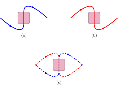
Figure 1: A bidirectional device, such as a half-wave plate or a quarter-wave plate, can be used in two alternative modes: a forward mode (corresponding to the blue path in subfigure (a)), and a backward mode (corresponding to the red path in subfigure (b)). Quantum control over the system travelling through the device can be used to create a coherent superposition of the forward and backward mode (subfigure (c)), giving rise to scenarios where the roles of the input and output ports of the device becomes indefinite.

A recent example of a new foundational concept is the concept of indefinite time direction (36). This notion was originally motivated by questions about the arrow of time, including whether it is in principle possible to conceive quantum processes that receive their inputs in the future and produce their outputs in the past, and whether it is in principle possible to conceive situations where the time order between the inputs and the outputs of a quantum process is indefinite. The study of these foundational questions led to a broader notion of indefinite input-output direction, which applies to any scenario involving bidirectional processes (36), that is, processes for which the roles of the input and the output ports can be exchanged. Examples of bidirectional processes are the processes induced by half-wave plates, quarter-wave plates, and other optical crystals that rotate the polarisation of single photons. Any such crystal can be traversed in two opposite directions, e.g. from bottom to top or from top to bottom, as in Fig. 1. The two opposite ways of traversing the crystal give rise to two different quantum processes, related by a symmetry transformation called input-output inversion (36). Conventionally, we can call one process the forward process and the other process the backward process. Forward and backward processes can be also probed in a coherent quantum superposition, by controlling a photon’s trajectory through the crystal, as illustrated in Fig. 1. As a result, the direction of the information flow within the crystal can become indefinite.

A general mathematical framework for describing the use of a bidirectional device in an indefinite input-output direction was provided in Ref. (36). The framework includes operations that generate a coherent superposition of forward and backward processes, as well as more general operations, therein called operations with indefinite time direction. The reason for the name is that Ref. (36) considered foundational scenarios where the two ports of a bidirectional device are associated to two specific moments of time $t_{1}$ and $t_{2}>t_{1}$, so that the “forward process” would be the process with inputs entering in the past (at time $t_{1}$) and output exiting in the future (at time $t_{2}$), while the “backward process” would be the process for which the roles of past and future are exchanged. Here, instead, we will use the more neutral term quantum operations indefinite input-output direction, to stress that the framework applies also to scenarios in which the input and output ports are not associated to specific moments of time.

A first operational consequence of input-output indefiniteness was shown in Ref. (36), which provided a quantum game in which the player can win with certainty only if the input-output direction is indefinite. Recently, this game was demonstrated experimentally with photons (37; 38). Another consequence can be deduced from a related work on the quantum superposition of thermodynamic processes with opposite time arrows (39). Besides these works, however, the operational consequences of indefinite input-output direction are still largely unexplored, especially in comparison to those of indefinite causal order, which have been extensively investigated in the past decade (40; 35; 41; 42; 43; 44; 45; 19; 46; 47; 48; 49; 24; 26; 50; 51).

In this paper, we explore the consequences of input-output indefiniteness for the transmission of classical and quantum information through noisy channels. We formulate a communication model in which a sender transmits quantum particles to a receiver through a bidirectional device that acts in a coherent superposition of the forward and backward mode, as in Fig. 1. Specifically, we consider the basic scenario of a single particle travelling through a single quantum device, and we show that the ability to control the direction in which the particle traverses the device can increase the amount of classical and quantum information reaching the receiver. For dephasing noise, corresponding e.g. to rotations of a single photon’s polarisation about a fixed direction, we show that a perfect, deterministic transmission of quantum bits becomes possible even if the original dephasing channel was entanglement-breaking and therefore unable to transmit any quantum information. For more radical types of noise, such as depolarising noise, we show that indefinite input-output direction increases the classical channel capacity (i.e. the optimal rate at which the channel can reliably transmit classical bits) and the quantum channel capacity (i.e. the optimal rate at which the channel can transmit quantum bits). Notably, both capacities can be non-zero even in parameter regimes where no information can be transmitted by using the device in a fixed direction. For example, a completely depolarising qubit channel used in an indefinite input-output direction gives rise to a classical capacity of $0.3113$ bits per channel use, and even permits a noiseless heralded transmission of qubit states with a success probability of $25\%$.

Our results highlight some similarities, as well as some differences, between input-output indefiniteness and the related notions of indefinite causal order and indefinite trajectories. Regarding the similarities, the communication advantages observed in all these scenarios are consequences of the ability to coherently control the configuration of noisy channels, as first observed by Gisin et al (6) and recently elaborated in Refs. (7; 52). On the other hand, our results indicate that coherent control over the input-output direction can offer larger advantages. For example, putting two completely depolarising qubit channels on two alternative paths, and coherently controlling the path gives a classical capacity of at most 0.16 bits per channel use, while using the two channels in a coherently controlled order yields a capacity of at most 0.049 bits per channel use. Both values are strictly smaller than the classical capacity of 0.3113 bits per channel use achievable with a single depolarising channel used in a coherent superposition of the forward and backward mode.

Communication protocols exploiting input-output indefiniteness are also interesting outside the context of quantum communication. They can be regarded as a new type of error correction, boosted by coherent quantum control over the input-output direction of the noisy processes. These protocols have some similarity with dynamical decoupling protocols (53), in which an unknown evolution is alternated with its inverse in a sequence of time steps. In our protocols, however, the advantages do not come from alternation, but rather from the quantum interference between a forward process and the corresponding backward process. As we will see later in the paper, the working principle of our protocols appears to be the ability to distinguish between errors represented by symmetric matrices and errors represented by anti-symmetric matrices, which in particular allows one to correct Pauli $Y$ errors separately from the other types of single-qubit errors.

The rest of the paper is organised as follows. In Section II we introduce a communication model that uses bidirectional devices in a coherent superposition of the forward and backward directions. In Section III we apply our communication model to the special case of noisy channels that are invariant under transposition, which includes all the examples studied in the rest of the paper. The examples are provided in Section IV, where we show that input-output indefiniteness can boost the capacity of depolarising and dephasing channels. Finally, the conclusions are drawn in Section V.

II Communication model with superposition of input-output directions

II.1 Input-output inversion and superposition of input-output directions

Let us start by reviewing the notion of indefinite input-output direction introduced in Ref. (36). This notion applies to bidirectional quantum processes, that is, quantum processes for which roles of the input and output ports are exchangeable. For example, the transmission of a single photon through a half-wave plate is a bidirectional process, because the exchange of the entrance point of the photon with its exit point gives rise to a valid single-photon evolution.

The set of bidirectional quantum processes on a given quantum system was characterised in Ref. (36). There, it was shown that a process is bidirectional if and only if it is described by a bistochastic channel (54; 55), that is, a completely positive linear map $\mathcal{C}$ with a Kraus representation $\mathcal{C}(\cdot)=\sum_{i=1}^{r}C_{i}\cdot C_{i}^{\dagger}$ where the Kraus operators $\{C_{i}\}_{i=1}^{r}$ satisfy the normalisation condition $\sum_{i=1}^{r}C_{i}^{\dagger}C_{i}=\sum_{i=1}^{r}C_{i}C_{i}^{\dagger}=I$, $I$ being the identity matrix on the system’s Hilbert space.

A given bidirectional device is associated to a forward channel $\mathcal{C}$ (describing the transformation of the system’s density matrix in a given direction, conventionally regarded as the “forward” one) and to a backward channel $\Theta(\mathcal{C})$ (describing the transformation of the system’s density matrix in the opposite direction). The map $\Theta$ transforming the forward channel into the backward channel is called an input-output inversion. Ref. (36) showed that the possible input-output inversions are of the form $\Theta(\mathcal{C})(\cdot)=\sum_{i}\theta(C_{i})\cdot\theta(C_{i}^{\dagger})$, where the matrices $\theta(C_{i})$ are either unitarily equivalent to the transpose, namely

$$\theta(C_{i})=UC_{i}^{T}U^{\dagger}\,\qquad\forall i\in\{1,\dots,r\}$$ (1)

where $U$ is a fixed unitary matrix and $C_{i}^{T}$ is the transpose of $C_{i}$ in a fixed basis, or unitarily equivalent to the adjoint, namely

$$\theta(C_{i})=UC_{i}^{\dagger}U^{\dagger}\,,\qquad\forall i\in\{1,\dots,r\}\,,$$ (2)

where $C_{i}^{\dagger}$ is the adjoint (conjugate transpose) of $C_{i}$. A fundamental difference between the transpose and the adjoint is that the transpose can in principle be applied locally to part of a bipartite quantum channel, whereas the adjoint cannot, because it would generally give rise to maps that are not completely positive (36). Technically, the difference is that the transpose is an admissible transformation of quantum channels (an admissible quantum supermap, in the language of (56)), while the adjoint is not. In the following, we will focus our attention to bidirectional devices for which the input-output inversion is unitarily equivalent to the transpose. Example are photonic devices, such as half-wave plates and other polarisation rotators, or Stern-Gerlach devices.

Another example of input-output inversion is time reversal (57; 58). An extended discussion of this example is provided in (36), and here we only sketch the main ideas for the reader’s convenience. The standard approach to time reversal, dating back to Winger (57), is to define an anti-unitary operation $T$ acting on quantum states. The operator $T$ is generally taken to represent the change of description due to the inversion of time coordinate $t\mapsto-t$. Now, the time reversal of quantum states implicitly defines a time reversal of unitary evolutions: if a unitary evolution $U_{t_{0},t_{1}}$ transforms the state $|\psi\rangle$ at time $t_{1}$ into the state $U_{t_{1},t_{2}}|\psi\rangle$ at time $t_{2}>t_{1}$, then the time-reversed evolution should transform the state $TU_{t_{1},t_{2}}|\psi\rangle$ at time $-t_{2}$ into the state $T|\psi\rangle$ at time $-t_{1}$. Since this condition should hold for every state $|\psi\rangle$, setting $|\varphi\rangle:=TU_{t_{1},t_{2}}|\psi\rangle$ we obtain that the time-reversed evolution, denoted by $\theta(U_{t_{1},t_{2}})$, must transform the state $|\varphi\rangle$ into the state $TU_{t_{1},t_{2}}^{\dagger}T^{-1}|\varphi\rangle$. Hence, the time-reversed evolution is $\theta(U_{t_{1},t_{2}})=TU_{t_{1},t_{2}}^{\dagger}T^{-1}$. This expression is consistent with Eq. (1): by decomposing anti-unitary operator as $T=UK$, where $U$ is a unitary operator and $K$ is the complex conjugation, we obtain the expression $\theta(U_{t_{1},t_{2}})=U\,U_{t_{1},t_{2}}^{T}\,U^{\dagger}$, meaning that time reversal of the unitary evolution $U_{t_{1},t_{2}}$ is unitarily equivalent to its transpose $U_{t_{1},t_{2}}^{T}$. The above argument can be extended from unitary channels to general bistochastic channels by using the fact that bistochastic channels are linear combinations of unitary channels (see (36) for more details). In summary, the canonical time reversal in quantum theory is associated to an input-output inversion that is unitarily equivalent to the transpose. Furthermore, the combination of time reversal with other symmetries, such as charge conjugation $C$ and parity inversion $P$, gives rise to other examples of input-output inversions, such as those corresponding to the symmetries $CT$, $PT$, and $CPT$. More generally, an input-output inversion involves the exchange of two ports of a quantum device, without necessarily associating the two ports to two specific moments of time $t_{1}$ and $t_{2}$.

Traditionally, the roles of the input and output ports of quantum devices have been taken to be fixed. In general, however, the user is free to choose which port serves as the input and which one serves as the output, and the choice can even be controlled by the state of a quantum system. The ability to control the input-output direction of the information flow within a given device is described by a higher order transformation, called the quantum time flip (36). The quantum time flip takes as input a bistochastic quantum channel $\mathcal{C}$, and produces as output another bistochastic quantum channel $\mathcal{F}(\mathcal{C})$, acting on the original quantum system (hereafter called the target) and on a control qubit, which determines the input-output direction. The channel $\mathcal{F}(\mathcal{C})$ can be specified via its Kraus representation, given by $\mathcal{F}(\mathcal{C})(\cdot)=\sum_{i}F_{i}\cdot F_{i}^{\dagger}$ with

$$F_{i}=C_{i}\otimes|0\rangle\langle 0|+C_{i}^{T}\otimes|1\rangle\langle 1|\quad i\in\{1,\cdots,r\}\,.$$ (3)

If the control system is set to $|0\rangle$, then the action of the channel $\mathcal{F}(\mathcal{C})$ on the target system is given by the forward channel $\mathcal{C}$ (Fig. 1(a)); if instead the control system is set to $|1\rangle$, then the action on the target is given by the backward channel $\mathcal{C}^{T}$ (Fig. 1(b)). Indefiniteness of the input-output direction arises when the control system is set to a coherent superposition of $|0\rangle$ and $|1\rangle$, such as e.g. the maximally coherent state $|+\rangle=(|0\rangle+|1\rangle)/\sqrt{2}$. In this case, the channel $\mathcal{F}(\mathcal{C})$ can be regarded as a coherent superposition of the forward and backward channels $\mathcal{C}$ and $\mathcal{C}^{T}$, in the sense of Ref. (4; 59; 60; 5; 5; 61; 62; 63; 64; 65; 66; 9; 6; 7; 8; 10; 52; 22; 26) (Fig. 1(c)).

II.2 Communication through a single bistochastic channel in an indefinite input-output direction

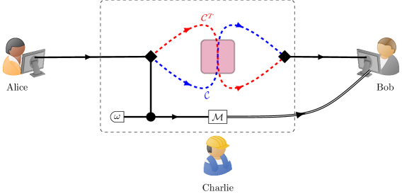
Figure 2: Communication model using channels in an indefinite input-output direction. A sender, Alice, transmits quantum states to a receiver, Bob, with the assistance of a third party Charlie. The overall channel connecting Alice to Bob is represented by the dashed black box in the figure, with the black solid line on the left representing Alice’s input to the channel, the black solid line on the right representing the channel’s output received by Bob, and the double black line on the left representing the transmission of classical information from Charlie to Bob. Inside the box, Alice’s input is routed on two possible paths, traversing a device (pink box) depending on the state of a control system (black line below the pink box). One path (dashed blue line) traverses the device in the forward direction (from bottom to top) and is associated to the channel $\mathcal{C}$. The other path (dashed red line) traverses the device in the backward direction (from top to bottom) and is associated to the channel $\mathcal{C}^{T}$. The control system is initialised by Charlie in a fixed state $\omega$, independently on the quantum states used by the sender to transmit information to the receiver. At the end, Charlie performs a measurement $\mathcal{M}$ on the control system and communicates his measurement outcome to Bob via a classical communication channel.

We now develop a model of quantum communication using bidirectional devices in an indefinite input-output direction. The model is illustrated in Fig. 2. A sender (Alice) wants to transmit a quantum state $\rho$ to a receiver (Bob). To this purpose, Alice uses a bidirectional device that acts as channel $\mathcal{C}$ when traversed in a given direction and as channel $\mathcal{C}^{T}$ when traversed in the opposite direction. A third party, Charlie, controls the direction in which Alice’s particle traverses the device, thereby realising the quantum time flip $\mathcal{F}$ operation described in the previous subsection. At the beginning of the protocol, Charlie initialises the control qubit in a quantum state $\omega$. Then, the target and control, initially in the product state $\rho\otimes\omega$, undergo the joint evolution described by the quantum channel $\mathcal{F}(\mathcal{C})$, thereby evolving into the state $[\mathcal{F}(\mathcal{C})](\rho\otimes\omega)$. At this point, Charlie performs a measurement $\mathcal{M}$ on the control system and communicates the outcome to Bob via a classical communication channel. Finally, Bob tries to retrieve Alice’s input state $\rho$, using the classical information provided by Charlie.

The above communication model can be applied to different communication tasks, including the communication of classical data (in which case the input state $\rho$ is chosen from a set of states $\{\rho_{x}\}_{x\in\mathsf{X}}$ used to encoded a message $x$ from some finite alphabet $\mathsf{X}$) and the communication of quantum data (in which case the input state $\rho$ is an arbitrary density matrix with support contained in a suitable subspace). In turn, the communication of quantum data can be used for a number of applications, including for example quantum key distribution (1; 2) or quantum secure direct communication (67; 68; 69)

Let us now analyze explicitly the steps of our communication protocol. At the beginning, the target system is in the state $\rho$ and the control system is in the state $\omega$. Then, the two states are sent through the channel $\mathcal{F}(\mathcal{C})$. The effective evolution from Alice’s input state $\rho$ to the joint output state of the target and control is given by a channel $\mathcal{F}_{\omega}(\rho)$, defined as

$$\left[\mathcal{F}_{\omega}(\mathcal{C})\right](\rho) :=[\mathcal{F}(\mathcal{C})]\,(\rho\otimes\omega)$$

$$=\sum_{i=1}^{r}\Big{\{}\frac{C_{i}+C_{i}^{T}}{2}\,~{}\rho~{}\frac{C_{i}^{\dagger}+\overline{C}_{i}}{2}\otimes\omega+\frac{C_{i}-C_{i}^{T}}{2}\,~{}\rho~{}\frac{C_{i}^{\dagger}-\overline{C}_{i}}{2}\otimes Z\omega Z$$

$$\qquad+\frac{C_{i}+C_{i}^{T}}{2}\,~{}\rho~{}\frac{C_{i}^{\dagger}-\overline{C}_{i}}{2}\otimes\omega Z+\frac{C_{i}-C_{i}^{T}}{2}\,~{}\rho~{}\frac{C_{i}^{\dagger}+\overline{C}_{i}}{2}\otimes Z\omega\Big{\}}\,,$$ (4)

where $(C_{i})_{i=1}^{r}$ is a Kraus representation of the channel $\mathcal{C}$, $\overline{C}_{i}:=\left(C_{i}^{T}\right)^{\dagger}$ is the complex conjugate of the matrix $C_{i}$, and $Z:=|0\rangle\langle 0|-|1\rangle\langle 1|$ is the Pauli $z$ matrix. Here, the second equality follows by substituting the expressions $|0\rangle\langle 0|=(I+Z)/2$ and $|1\rangle\langle 1|=(I-Z)/2$ into Eq. (3). The channel $\mathcal{F}_{\omega}(\mathcal{C})$ describes the use of a bidirectional device in a combination of the forward and backward directions determined by the quantum state $\omega$. In the following, we will call $\mathcal{F}_{\omega}(\mathcal{C})$ the flipped channel.

The next step in the protocol is Charlie’s measurement on the control qubit. The measurement can be described by a quantum-to-classical channel $\mathcal{M}$, of the form

$$\mathcal{M}(\rho)=\sum_{j=1}^{N}\,|j\rangle\langle j|\,\operatorname{Tr}[P_{j}\rho]\,,$$ (5)

where $(P_{j})_{j=1}^{N}$ is a positive operator-valued measure (POVM) and $\{|j\rangle\}_{j=1}^{N}$ are orthogonal states of a classical system, on which the measurement outcome is recorded.

After Charlie’s measurement, the target system and the classical system end up in the quantum-classical state

$$\rho_{\rm target,classical}=(\mathcal{I}_{\rm target}\otimes\mathcal{M})[\mathcal{F}(\mathcal{C})]\,(\rho\otimes\omega)=(\mathcal{I}_{\rm target}\otimes\mathcal{M})[\mathcal{F}_{\omega}(\mathcal{C})]\,(\rho)\,,$$ (6)

where $\mathcal{I}_{\rm target}$ is the identity map acting on the target system. Finally, Charlie communicates to Bob the outcome of his measurement via a classical communication channel. Hence, the classical system at the output of channel $\mathcal{M}$ is eventually in Bob’s laboratory.

Overall, the flow of information from Alice to Bob is described by the effective channel

$$\mathcal{C}_{\rm eff}:=(\mathcal{I}_{\rm target}\otimes\mathcal{M})\mathcal{F}_{\omega}(\mathcal{C}).$$ (7)

The goal of this paper is the study of the classical and quantum capacities of the effective channel $\mathcal{C}_{\rm eff}$, optimised over all possible state preparations $\omega$ and over all possible measurements $\mathcal{M}$.

II.3 Relations with other communication models in the literature

To better understand our communication model, it is useful to consider its similarities and differences with other models considered in the literature. First, it is important to observe that our model is different from two-way communication models in which information travels simultaneously from Alice to Bob and from Bob to Alice (70; 71; 72), or from related models of multiple access quantum communication channels (73; 74). Unlike these models, our model does not exhibit any indefiniteness in the roles of sender and receiver, but only in the direction in which the sender’s messages traverse a given quantum device.

Second, it is important to clarify the role of the third party, Charlie. In our model, one can think of Charlie as a communication provider, who assists Alice and Bob, without interfering with Alice’s choice of input states. Accordingly, Charlie initialises the control system in fixed quantum state $\omega$, independent of the quantum states sent by Alice. This setting is broadly assumed in other communication models based on superposition of channels (52; 7; 8; 13).

It is also worth noting that Charlie’s assistance is limited to the transmission of classical information. This constraint is similar to the constraint adopted in the study of quantum communication with the assistance of classical information from the environment (75; 76), with the only difference that in our case we do not assume assistance from the whole environment of the channel between Alice and Bob, but only from a two-dimensional system that controls the direction of the information flow within a given device.

On a more formal level, one can regard our communication model as part of a resource theory (77). More specifically, our model is an instance of a resource theory of quantum communication (52), in which communication devices are assembled by the communication provider to build an effective communication channel connecting the sender to the receiver. In this framework, the operations performed by the communication provider are described by quantum supermaps (35; 56; 78; 79), that is, higher order operations that take in input the quantum channels associated to the initial devices, and produce in output a new quantum channel connecting the sender to the receiver.

The supermaps implementable by the communication provider are called free, in the sense that they are regarded as achievable in the resource theory under consideration. Often, free operations are motivated by practical constraints arising in real-world applications. Note, however, that in general this needs not be the case: the resource-theoretic framework is useful not only as a way to analyze practical constraints, but also as a theoretical lens for understanding the power of certain sets of operations, conventionally referred to as “free” even though they are not necessarily easy to implement.

Different resource theories of communication correspond to different choices of free supermaps. For example, standard quantum Shannon theory can be formulated as a resource theory of communication where the free supermaps combine the original devices in a well-defined configuration, typically in parallel and without the addition of any other channel on the side (52). Various extension of standard quantum Shannon theory can be obtained by enlarging the set of free operations, e.g. by including the ability to connect quantum channels in a coherent superposition of orders (11; 12; 13; 14; 15; 16; 20) or to coherently control which quantum channel is used to transmit information (7; 8). Communication advantages over standard quantum Shannon theory can then be understood as a result of the enlargement of the set of free supermaps, corresponding to more general ways to assemble the initial devices into an effective channel connecting the sender to the receiver.

The communication model considered in this paper corresponds to a new way to enlarge the set of free supermaps, including the possibility of using bidirectional devices in a coherent superposition of two alternative directions. As we will see later in the paper, this enlargement provides some interesting advantages over the standard model of quantum Shannon theory. On the other hand, the model still satisfies a constraint put forward in Ref. (52): free operations should not allow Alice and Bob to communicate independently of the initial devices used by Charlie to set up the communication link between them. The proof that our communication model satisfies this constraint is provided in Appendix A.

III Communication through transposition invariant channels

All the concrete examples of noisy channels studied in this paper are invariant under transposition, namely $\mathcal{C}^{T}=\mathcal{C}$. For this class of channels we now derive Charlie’s optimal state preparation $\omega$ and optimal measurement $\mathcal{M}$.

Let us start from a characterisation of the transposition invariant channels:

Proposition 1.

The following are equivalent:

1. $\mathcal{C}^{T}=\mathcal{C}$.

2. There exists a Kraus representation $\mathcal{C}(\rho)=\sum_{i}C_{i}\rho C_{i}^{\dagger}$ in which each Kraus operator $C_{i}$ is either symmetric ($C_{i}^{T}=C_{i}$) or anti-symmetric ($C_{i}^{T}=-C_{i}$).

The proof is provided in Appendix B.

For a transposition invariant channel, the forward and backward processes coincide. Nevertheless, quantum interference between these two processes gives rise to non-trivial effects. This fact can be seen from Eq. (4), which in the case of transposition invariant channels becomes

$$\big{[}\mathcal{F}_{\omega}(\mathcal{C})\big{]}\,(\rho)= \sum_{i\in\mathsf{S}_{\rm sym}}C_{i}\rho C_{i}^{\dagger}\otimes\omega+\sum_{i\in\mathsf{S}_{\rm anti}}C_{i}\rho C_{i}^{\dagger}\otimes Z\omega Z\,,$$ (8)

where $\mathsf{S}_{\rm sym}:=\{i~{}|~{}C_{i}^{T}=C_{i}\}$ is the set of indices corresponding to symmetric Kraus operators and $\mathsf{S}_{\rm anti}:=\{i~{}|~{}C_{i}^{T}=-C_{i}\}$ is the set of indices corresponding to antisymmetric Kraus operators.

Eq. (8) tells us that the interference between the two input-output directions separates the symmetric and anti-symmetric Kraus operators of the channel $\mathcal{C}$, correlating the symmetric operators with the state $\omega$, and the anti-symmetric operators with the state $Z\omega Z$. In particular, if the control state $\omega$ is initially set to the maximally coherent state $\omega=|+\rangle\langle+|$, then the output state is

$$\big{[}\mathcal{F}_{|+\rangle\langle+|}(\mathcal{C})\big{]}\,(\rho)=\sum_{i\in\mathsf{S}_{\rm sym}}C_{i}\rho C_{i}^{\dagger}\otimes|+\rangle\langle+|+\sum_{i\in\mathsf{S}_{\rm anti}}C_{i}\rho C_{i}^{\dagger}\otimes|-\rangle\langle-|\,,$$ (9)

having used the notation $|\pm\rangle:=(|0\rangle+\pm|1\rangle)/\sqrt{2}$. Eq. (9) shows that the symmetric and anti-symmetric part of channel $\mathcal{C}$ can be perfectly separated by measuring the control on the orthonormal basis $\{|+\rangle,|-\rangle\}$.

The above observations provide the optimal strategy for Charlie to assist Alice and Bob:

Proposition 2.

Let $\mathcal{C}$ be a transposition invariant channel. For every communication task in the model of Fig. 2, one can assume without loss of generality that

1. the control system is initialised in the maximally coherent state $\omega=|+\rangle\langle+|$, and

2. the control system is measured on the Fourier basis $\{|+\rangle,|-\rangle\}$, corresponding to the quantum-to-classical channel $\mathcal{M}_{\rm Fourier}(\rho)=|+\rangle\langle+|\,\langle+|\rho|+\rangle+|-\rangle\langle-|\,\langle-|\rho|-\rangle$.

Proof. The proof is a straightforward consequence of Eqs. (8) and (9).

Item 1 follows from the fact that Charlie can always obtain the output state in Eq. (8) from the output state in Eq. (9) by applying a local operation on the control system: Charlie only needs to measure the control system in the Fourier basis $\{|+\rangle,|-\rangle\}$ and to reset the control system to either the state $\omega$ or to the state $Z\omega Z$, depending on whether the measurement outcome is $+$ or $-$, respectively.

Item 2 follows from the fact that, for the optimal input state $\omega=|+\rangle\langle+|$, the output state $[\mathcal{F}_{\omega}(\mathcal{C})](\rho)$ is invariant under the action of the classical-to-quantum channel $\mathcal{M}_{\rm Fourier}$. Hence, transmitting the outcome of the Fourier basis measurement to Bob is equivalent to transmitting the state of the control qubit. Any other measurement $\mathcal{M}$ that Charlie could have performed instead of the Fourier measurement can then be performed by Bob as part of his decoding operations. $\blacksquare$

Thanks to Proposition 2, we can assume without loss of generality that the control system is initialised in the maximally coherent state $\omega=|+\rangle\langle+|$ and measured in the Fourier basis. In this case, the effective channel $\mathcal{C}_{\rm eff}$ in Eq. (7) is simply given by

$$\mathcal{C}_{\rm eff}:=\mathcal{F}_{|+\rangle\langle+|}(\mathcal{C})\,.$$ (10)

In the next section, we will study the classical and quantum communication capacities of the channel $\mathcal{F}_{|+\rangle\langle+|}(\mathcal{C})$ in the case of qubit depolarising and dephasing channels. Before doing that, we now review the basic notions on classical and quantum channel capacities, and the relation of the latter with the transmission of private classical information. Readers who are already familiar with these notions can skip directly to the next section.

The classical capacity of a given noisy channel $\mathcal{N}$ is operationally defined as the maximum number of classical bits one can reliably transmit per use of the channel $\mathcal{N}$ in the asymptotic limit of many parallel uses. The relevant quantity for the calculation of the classical capacity is the Holevo information of the channel $\mathcal{N}$ (80), defined as

$$\chi(\mathcal{N}):=\max_{(p_{x},\rho_{x})_{x\in\mathsf{X}}}H\left(\mathcal{N}\left(\sum_{x\in\mathsf{X}}p_{x}\,\rho_{x}\right)\,\right)-\sum_{x\in\mathsf{X}}p_{x}\,H\big{(}\mathcal{N}(\rho_{x})\big{)}\,,$$ (11)

where $H(\rho)=-\operatorname{Tr}[\rho\log\rho]$ is the von Neumann entropy of an arbitrary state $\rho$, and the maximisation runs over all possible ensembles $\{p_{x},\rho_{x}\}_{x\in\mathsf{X}}$ consisting of density matrices $\rho_{x}$ given with probabilities $p_{x}$.

As a consequence of the Holevo-Schumacher-Westmoreland theorem (80; 81), the classical capacity is given by

$$C(\mathcal{N}):=\lim_{k\to\infty}\frac{\chi(\mathcal{N}^{\otimes k})}{k}\,.$$ (12)

Since the Holevo quantity is generally superadditive under tensor products, one generally has the bound

$$C(\mathcal{N})\geq\chi(\mathcal{N})\,,$$ (13)

valid for arbitrary quantum channels $\mathcal{N}$.

Let us consider now the quantum capacity, operationally defined as the maximum number of quantum bits one can reliably transmit per channel use in the asymptotic limit of many parallel uses of the channel $\mathcal{N}$. The relevant quantity for the calculation of the quantum capacity is the coherent information of the channel $\mathcal{N}$, defined as (82)

$$I_{\rm c}(\mathcal{N}):=\max_{\rho\in{\mathsf{St}}(A)}I_{\rm c}(\mathcal{N},\rho)\qquad{\rm with}\qquad I_{\rm c}(\mathcal{N},\rho):=H\big{(}\mathcal{N}(\rho)\big{)}-H\big{(}\,(\mathcal{N}\otimes\mathcal{I})(\Psi_{\rho})\,\big{)}\,,$$ (14)

where ${\mathsf{St}}(A)$ is the set of all possible density matrices of system $A$, the input system of channel $\mathcal{N}$, and $\Psi_{\rho}\in{\mathsf{St}}(A\otimes R)$ is an arbitrary purification of the state $\rho$, namely a pure state of a composite system $A\otimes R$ (with a suitable reference system $R$) such that $\rho=\operatorname{Tr}_{R}[\Psi_{\rho}]$.

The Lloyd-Shor-Devetak theorem (83; 84; 85) shows that the quantum capacity is given by

$$Q(\mathcal{N})=\lim_{n\to\infty}\frac{I_{\rm c}(\mathcal{N}^{\otimes n})}{n}$$ (15)

Since in general the coherent information is superadditive under tensor products, one has the lower bound

$$Q(\mathcal{N})\geq I_{\rm c}(\mathcal{N})\,,$$ (16)

valid for every quantum channel $\mathcal{N}$.

In turn, the quantum capacity is a lower bound to the private capacity $P(\mathcal{N})$ of the channel $\mathcal{N}$, defined as the maximum number of classical bits that the sender can privately transmit to the receiver per channel use in the asymptotic limit of many parallel uses. The relevant quantity for the calculation of the private capacity is the private information of the channel $\mathcal{N}$, defined as (85)

$$I_{\rm p}(\mathcal{N})=\max_{(p_{x},\rho_{x})_{x\in\mathsf{X}}}\left\{\,I_{\rm c}\left(\mathcal{N},\sum_{x\in\mathsf{X}}p_{x}\,\rho_{x}\right)-\sum_{x\in\mathsf{X}}p_{x}\,I_{\rm c}(\mathcal{N},\rho_{x})\right\}\,,$$ (17)

where the maximisation is over all possible input ensembles $(p_{x},\rho_{x})_{x\in\mathsf{X}}$.

Explicitly, the private capacity is given by (85)

$$P(\mathcal{N})=\lim_{n\to\infty}\frac{I_{\rm p}(\mathcal{N}^{\otimes n})}{n}\,,$$ (18)

and one has the bound

$$P(\mathcal{N})\geq Q(\mathcal{N})\,.$$ (19)

The intuitive reason for the bound (19) is that the channel $\mathcal{N}$ can be used to send private classical messages by encoding them into quantum states, as it is done, for example, in the protocols of quantum secure direct communication (67; 68; 69). Hence, the rate at which quantum states can be transmitted reliably provides a lower bound to the rate at which classical messages can be transmitted reliably and privately.

In the following, we will use the lower bounds (13) and (16) to estimate the classical and quantum capacities of the effective channel $\mathcal{C}_{\rm eff}$ arising from the use of a bistochastic channel $\mathcal{C}$ in an indefinite input-output direction.

IV Communication advantages of indefinite input-output direction

Here we apply our communication model to two concrete examples of noisy qubit channels: depolarising channels and dephasing channels. In both examples, we will observe advantages of input-output indefiniteness in the transmission of classical and quantum data with respect to the basic scenario where the channels are used in a definite direction.

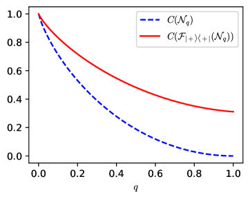
Figure 3: Classical capacity enhancement for qubit depolarising channels. The lower line (blue, dashed) and top line (red, solid) represent the classical capacity of $\mathcal{N}_{q}$ and the effective channel $\mathcal{F}_{|+\rangle\langle+|}(\mathcal{N}_{q})$, respectively, for all possible values of the depolarisation probability $q$.

IV.1 Enhanced transmission of classical information through depolarising channels

A qubit depolarising channel with depolarisation probability $q$ is a linear map $\mathcal{N}_{q}:M_{2}(\mathbb{C})\to M_{2}(\mathbb{C})$ of the form

$$\mathcal{N}_{q}(\rho) =q\,\frac{I}{2}+(1-q)\rho$$

$$=\left(1-q+\frac{q}{4}\right)\,\rho+\frac{q}{4}\,(X\rho X+Y\rho Y+Z\rho Z)\,,$$ (20)

where $X,Y,Z$ are the three Pauli matrices. Like all Pauli channels, the depolarising channel is bistochastic and invariant under transposition.

Now, suppose that Charlie uses a depolarising channel to set up a communication link between Alice and Bob, as in the model of Fig. 2. Charlie’s optimal strategy, provided by Proposition 2, results into the effective channel (10), which in this case reads

$$\big{[}\mathcal{F}_{|+\rangle\langle+|}(\mathcal{N}_{q})\big{]}\,(\rho)=\left(1-\frac{q}{4}\right)\mathcal{C}_{+}(\rho)\otimes|+\rangle\langle+|+\frac{q}{4}\,\mathcal{C}_{-}(\rho)\otimes|-\rangle\langle-|\,,$$ (21)

with

$$\mathcal{C}_{+}(\rho):=\frac{4(1-q)\,\rho+q(\rho+X\rho X+Z\rho Z)}{4-q}\qquad{\rm and}\qquad\mathcal{C}_{-}(\rho):=Y\rho Y\,.$$ (22)

We now compare the classical capacities of the channels $\mathcal{N}_{q}$ and $\mathcal{F}_{|+\rangle\langle+|}(\mathcal{N}_{q})$. The classical capacity of channel $\mathcal{N}_{q}$ is well-known (86), and is given by

$$C(\mathcal{N}_{q})=1+\left(1-\frac{q}{2}\right)\log\left(1-\frac{q}{2}\right)+\frac{q}{2}\log\left(\frac{q}{2}\right)\,,$$ (23)

where $\log$ denotes the logarithm in base 2.

The classical capacity of the channel $\mathcal{F}_{|+\rangle\langle+|}(\mathcal{N}_{q})$ is derived in Appendix C, where we also address the case of general target systems of dimension $d\geq 2$. There, we prove that the classical capacity of the channel $\mathcal{F}_{|+\rangle\langle+|}(\mathcal{N}_{q})$ is a convex combination of the capacities of the channels $\mathcal{C}_{+}$ and $\mathcal{C}_{-}$, and takes the value

$$C\big{(}\mathcal{F}_{|+\rangle\langle+|}(\mathcal{N}_{q})\big{)}=C(\mathcal{N}_{q})-\frac{q}{4}\,\log q-\left(1-\frac{q}{4}\right)\log\left(1-\frac{q}{4}\right)\,.$$ (24)

This equation shows that the classical capacity $C\big{(}\mathcal{F}_{|+\rangle\langle+|}(\mathcal{N}_{q})\big{)}$ is strictly larger than the classical capacity of the original depolarising channel $\mathcal{N}_{q}$ for every positive value of the depolarisation probability. A comparison between the capacities of the two channels is illustrated in Fig. 3. In the most extreme case, $q=1$, input-output indefiniteness in the channel $\mathcal{F}_{|+\rangle\langle+|}(\mathcal{N}_{1})$ permits communication with a capacity of $0.3113$ bits per channel use, even if the original channel $\mathcal{N}_{1}$ has zero classical capacity.

The $0.3113$ capacity achieved with input-output indefiniteness can be compared with the maximum capacity achievable by other communication protocols using coherent superpositions of configurations. For example, when two completely depolarising channels are used in a superposition of two alternative orders, the maximum classical capacity is 0.049 bits (43; 19). If instead two completely depolarising channels are placed on two alternative paths, and a quantum particle is sent through these paths in a quantum superposition, then the maximum classical capacity is $0.16$ bits (87; 10). Remarkably, comparison between these setups shows that a single channel in a superposition of two input-output directions can offer larger benefits than two channels in a superposition of two orders, or in a superposition of two paths.

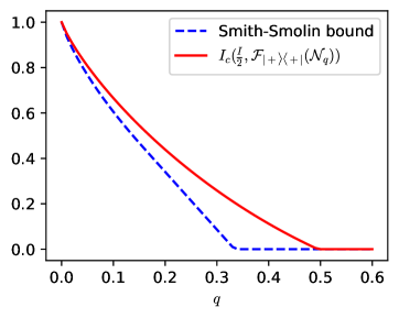
Figure 4: Quantum capacity enhancement for the qubit depolarising channel $\mathcal{N}_{q}$. The lower line (blue, dashed) represents the Smith-Smolin upper bound on $Q(\mathcal{N}_{q})$. The top line (red, solid) represents the coherent information of the effective channel $\mathcal{F}_{|+\rangle\langle+|}(\mathcal{N}_{q})$ when acting on the the maximally mixed state $\frac{I}{2}$. This value serves as a lower bound of $Q(\mathcal{F}_{|+\rangle\langle+|}(\mathcal{N}_{q}))$.

IV.2 Enhanced transmission of quantum information through depolarising channels

We now consider the transmission of quantum data through depolarising channels in a superposition of input-output directions. One challenge here is that no close-form expression for the quantum capacity of the depolarising channel has been found up to date. In order to establish an advantage of input-output indefiniteness, we will use an upper bound on the quantum capacity, derived by Smith and Smolin in Ref. (88). There, they showed that the quantum capacity $Q(\mathcal{N}_{q})$ is upper bounded as

$$Q(\mathcal{N}_{q})\leq\operatorname{co}\left[1-H(p),H\left(\frac{1-\gamma(p)}{2}\right)-H\left(\frac{\gamma(p)}{2}\right),1-4p\right]\,,$$ (25)

where $p=3q/4$, $\gamma(p)=4\sqrt{1-p}(1-\sqrt{1-p})$, $H(p)=-p\log p-(1-p)\log(1-p)$ and $\operatorname{co}[f_{1}(p),\cdots,f_{n}(p)]$ denotes the maximal convex function that is less than or equal to all $f_{i}(p)$, $i=1,\cdots,n$.

We now compare this upper bound with a lower bound on the quantum capacity of the effective channel $\mathcal{F}_{|+\rangle\langle+|}(\mathcal{N}_{q})$. By Eq. (16), the quantum capacity $Q(\mathcal{F}_{|+\rangle\langle+|}(\mathcal{N}_{q}))$ is lower bounded by the coherent information $I_{\rm c}(\mathcal{F}_{|+\rangle\langle+|}(\mathcal{N}_{q}))$, which in turn can be lower bounded by setting $\rho=I/2$ in Eq. (14). The resulting lower bound is

$$Q\big{(}\mathcal{F}_{|+\rangle\langle+|}(\mathcal{N}_{q})\big{)}\geq-\left(1-\frac{q}{4}\right)\log\left(\frac{1}{2}-\frac{q}{8}\right)-\frac{q}{4}\,\log\left(\frac{q}{8}\right)+\frac{3q}{4}\,\log\left(\frac{q}{4}\right)+\left(1-\frac{3q}{4}\right)\log\left(1-\frac{3q}{4}\right)\,.$$ (26)

The derivation of this equation is provided in Appendix D, where we also extend the bound to general quantum systems of dimension $d\geq 2$.

Comparing Eqs. (25) and (26), we obtain that the strict inequality $Q\big{(}\mathcal{F}_{|+\rangle\langle+|}(\mathcal{N}_{q})\big{)}>Q(\mathcal{N}_{q})$ is valid for every value of $q$ in the interval $(0,0.495)$. Our lower bound on the quantum capacity is plotted in Fig. 4, along with the Smith-Smolin upper bound on the quantum capacity of the depolarising channel.

When the depolarising probability reaches the value $q=1/3$, the Smith-Smolin bound implies that the quantum capacity of the depolarising channel $\mathcal{N}_{q}$ is zero. In contrast, our lower bound shows that the quantum capacity of the flipped depolarising channel $\mathcal{F}_{|+\rangle\langle+|}(\mathcal{N}_{q})$ is at least 0.2063 qubits at $q=1/3$, and remains larger than zero until $q$ is approximately $0.5$.

Note that a non-zero quantum capacity also implies a non-zero private capacity $P\big{(}\mathcal{F}_{|+\rangle\langle+|}(\mathcal{N}_{q})\big{)}$, due to the bound (19). Hence, the flipped depolarising channel $\mathcal{F}_{|+\rangle\langle+|}(\mathcal{N}_{q})$ can be used to securely transmit private messages from Alice to Bob. Notably, the definition of private capacity guarantees that the transmission is secure even if the eavesdropper has access to the whole environment of the channel $\mathcal{F}_{|+\rangle\langle+|}(\mathcal{N}_{q})$, which includes in particular the case in which the eavesdropper has access to Charlie’s measurement outcome.

In summary, input-output indefiniteness offers the possibility to achieve a reliable transmission of quantum states starting from depolarising channels that have zero quantum capacity. Remarkably, this feature cannot be achieved by using two depolarising channels in a superposition of alternative orders: as shown in Ref. (19), the quantum capacity obtained by placing two depolarising channels in a superposition of orders is non-zero only if the quantum capacity of the original channels is non-zero. In contrast, the superposition of two alternative input-output directions permits quantum communication even with a single depolarising channel with zero quantum capacity.

The increase of quantum capacity from zero to nonzero enables the use of quantum key distribution (QKD) protocols, such as BB84 (1) and E91 (2), or the use of quantum secure direct communication (QSDC) protocols (67; 68; 69) to transmit private messages from the sender to the receiver (see also (89) for a recent experimental demonstration and (90; 91; 92) for recent theoretical developments on this topic). In principle, these protocols can be implemented by encoding the appropriate quantum states in the multipartite states that achieve the quantum capacity $Q\big{(}\mathcal{F}_{|+\rangle\langle+|}(\mathcal{N}_{q})\big{)}$. In practice, however, this approach is still challenging because the capacity-achieving encoding is not known in general, and may involve large multipartite states that are hard to implement. Fortunately, a simpler approach is also possible: indeed, the superposition of input-output directions also enables a noiseless heralded transmission of quantum data. As one can see from Eq. (21), the evolution of the target system is unitary whenever the control system is found in the state $|-\rangle$. This means that, when Bob receives the outcome -, he can retrieve the state of Alice’s qubit without any error. Such heralded transmission allows Alice and Bob to implement QKD and QSDC protocols using the quantum states of the original protocols, which are much simpler to realise compared to their encoded version.

IV.3 Perfect transmission of quantum information through dephasing channels

We now show a scenario where input-output indefiniteness enables a perfect, deterministic transmission of quantum information. Consider a qubit dephasing channel of the form

$$\mathcal{M}_{p}=(1-p)\rho+pY\rho Y\,.$$ (27)

In normal conditions, this channel $\mathcal{M}_{p}$ can be used to transmit a classical bit, by encoding it into an eigenstate of the Pauli-$Y$ gate. However, transmitting a quantum bit per channel use of $\mathcal{M}_{p}$ is impossible except in the extreme cases $p=0$ or $p=1$, in which the channel $\mathcal{M}_{p}$ is noiseless. Indeed, the quantum capacity of the dephasing channel $\mathcal{M}_{q}$ is (3)

$$Q(\mathcal{M}_{p})=Q^{(1)}(\mathcal{M}_{p})=1-H(p)\,,$$ (28)

and is strictly smaller than 1 for every $q\in(0,1)$. In stark contrast, we now show that using the channel $\mathcal{M}_{q}$ in a coherent superposition of the forward and backward direction yields a quantum capacity of 1 qubit per channel use, for every possible value of $q$.

Suppose that the depolarising channel $\mathcal{M}_{q}$ is used in the scenario of Fig. 2, with the control qubit initialised in the maximally coherent state $\omega$. The resulting channel $\mathcal{F}_{|+\rangle\langle+|}(\mathcal{M}_{p})$ can be easily computed from Eq. (9), which yields

$$\big{[}\mathcal{F}_{|+\rangle\langle+|}(\mathcal{M}_{p})\big{]}\,(\rho)=(1-p)\rho\otimes|+\rangle\langle+|+pY\rho Y\otimes|-\rangle\langle-|\,.$$ (29)

Using this channel, Alice can transmit a qubit to Bob deterministically and without error. To retrieve Alice’s input state $\rho$, Bob needs only to measure the control system in the Fourier basis $\{|+\rangle,|-\rangle\}$: if the measurement outcome is “$+$”, then Bob obtained $\rho$ directly; if the outcome is “$-$”, then Bob can apply Pauli-$Y$ gate to the state to recover $\rho$.

Summarising, the flipped channel $\mathcal{F}_{|+\rangle\langle+|}(\mathcal{M}_{p})$ offers an advantage over the original dephasing channel $\mathcal{M}_{p}$ for every value of the dephasing probability except $p=0$ and $p=1$. The most extreme advantage arises for $p=1/2$, when the original dephasing channel has zero quantum capacity.

The possibility of perfect quantum communication through zero-capacity channels was also observed for quantum communication with indefinite causal order (13), where it was later shown to enable a task called random-receiver quantum communication (20). The same task can be achieved also in the present scenario, using a single dephasing channel in a coherent superposition of two alternative input-output directions instead of two channels in a coherent superposition of two alternative orders.

V Conclusions

In this paper, we developed a communication model where bidirectional quantum devices can be used in an indefinite input-output direction, and we showed that this input-output indefiniteness can enhance the classical and quantum capacity of noisy channels. These enhancements are similar to those arising from indefiniteness of the path of quantum particles through noisy processes, or from indefinite of the order in which the noisy processes occur. On the other hand, input-output indefiniteness does not require the use of multiple channels, or the use of a given channel at multiple moments of time. Moreover, the results of this paper indicate that indefiniteness of the input-output direction generally offers stronger advantages compared to the above models. For example, a single completely depolarising channel used in a superposition of two directions can reach a classical capacity of 0.31 bits, while two completely depolarising channels can at most reach a capacity of $0.16$ bits when put on two alternative paths, and of $0.049$ bits when used in two alternative orders.

The study of quantum communication with indefinite input-output direction sheds light on the operational features of the recently introduced “quantum time flip” operation. In turn, the quantum time flip and other operations with indefinite input-output direction can be used as a mathematical framework to formulate hypothetical scenarios where the arrow of time is in a quantum superposition. While these scenarios are far from the currently known physics, and therefore necessarily speculative, they can help clarifying the consequences of basic quantum principles, when applied to unusual settings involving the order of events in time. For example, consider a thought experiment where two parties, Alice and Bob, operate inside two closed laboratories and interact with each other only through a quantum channel, used by Alice to send quantum states to Bob. If the channel is bidirectional and the laws of nature are time-symmetric, this scenario is in principle compatible with two different time orders between Alice’s and Bob’s operations: Alice and Bob could operate in the forward order (with Alice preparing input states in Bob’s past, and the signals propagating from Alice’s laboratory to Bob’s laboratory in the forward time direction) or in the backward order (with Alice preparing input states in Bob’s future, and the signals propagating from Alice’s laboratory to Bob’s laboratory in the backward time direction). More generally, the time order of Alice’s and Bob’s operations may be indefinite, as in the quantum time flip. This closed laboratory situation is analogue to the situation considered by Oreshkov, Costa, and Brukner in the study of indefinite causal order (93), with the only difference that here the causal order between Alice and Bob is well defined (Alice can send signals to Bob, but not vice-versa) while the time order is indefinite. While the physical realisation of these scenarios is currently an open problem, the mathematical framework of quantum operations with indefinite input-output direction provides a rigorous way to explore them at a conceptual level. In addition, the superposition of time directions can be simulated in table top experiments by coherently controlling the path of single photons, as envisaged in (36) and recently demonstrated in two experiments (37; 38).

Another direction of future research is the experimental demonstration of the communication scenarios explored in this paper. Notably, all our communication protocols can already be demonstrated with a simple adaptation of the photonic setups in Refs. (37; 38). Indeed, these setups reproduced the action of the quantum time flip on unitary qubit channels, by controlling the direction in which a single photon traverses an arbitrary polarisation rotator. By randomising the choice of unitary channel, one can then realise the flipped Pauli channels appearing in our paper. The experimental realisation of quantum communication with indefinite input-output direction is expected to contribute to the development of a toolbox for quantum control over the configuration of multiple quantum devices, which may prove technologically useful in a longer term.

In the shorter term, our work provides the starting point for a number of foundational explorations. First, an interesting direction is the investigation of scenarios where both the input-output direction and the causal order of multiple processes are subject to quantum indefiniteness. A mathematical framework for these more general operations was recently established in (36), but very little is currently known about their information-theoretic potential. The angle of quantum communication, explored in this paper, represents a promising approach to explore the capabilities of new operations with indefinite order and direction. Another interesting area of future research is the study of quantum thermodynamic tasks assisted by indefinite input-output direction. Recently, the communication advantages of indefinite causal order stimulated new research in quantum thermodynamics (45; 94; 95). Similarly, the communication advantages provided in this paper suggest new thermodynamic protocols where the input-output direction of one or more processes is indefinite.

VI Acknowledgements

The authors thank H.Kristjánsson for helpful discussions. This work is supported by the Hong Kong Research Grant Council through grant 17307719 and though the Senior Research Fellowship Scheme SRFS2021-7S02, by the Croucher Foundation, and by the ID No. 62312 grant from the John Templeton Foundation, as part of the ‘The Quantum Information Structure of Spacetime, Second phase (QISS 2)’ Project (The Quantum Information Structure of Spacetime (QISS), Second Phase - John Templeton Foundation). Research at the Perimeter Institute is supported by the Government of Canada through the Department of Innovation, Science and Economic Development Canada and by the Province of Ontario through the Ministry of Research, Innovation and Science. The opinions expressed in this publication are those of the authors and do not necessarily reflect the views of the John Templeton Foundation.

Appendix A Proof that the communication model in Fig. 2 does not allow for communication independently of the input channels

Here we show that our communication model does not contain side-channel generating operations, defined as follows:

Definition 1 (Side-channel generating operations).

Let $\mathsf{M}_{\rm free}\subset\mathsf{M}$ be the set of free supermaps in a given resource theory of communication, $\mathsf{M}$ being the set of all quantum supermaps. A supermap $\mathcal{S}\in\mathsf{M}$ generates a classical (quantum) side-channel if there exist two free supermaps $\mathcal{S}_{1}\in\mathsf{M}_{\rm free}$ and $\mathcal{S}_{2}\in\mathsf{M}_{\rm free}$ such that

$$(\mathcal{S}_{2}\circ\mathcal{S}\circ\mathcal{S}_{1})(\mathcal{C})=\mathcal{C}_{0}\,,$$ (30)

where $\mathcal{C}$ is an arbitrary input channel and $\mathcal{C}_{0}$ is a fixed quantum channel with non-zero classical (quantum) capacity.

In the following, we show that no supermap of the form (33) can generate a side-channel in the sense of Definition 1. Specifically, we will prove the following theorem:

Theorem 1.

For every supermap $\mathcal{S}$ of the form (33), if the supermap $\mathcal{S}$ satisfies the condition $\mathcal{S}(\mathcal{C})=\mathcal{C}_{0}$ for a fixed $\mathcal{C}_{0}$ and for every bistochastic channel $\mathcal{C}$, then $\mathcal{C}_{0}$ has zero classical (quantum) capacity.

To prove the theorem, we need to specify the set of free supermaps in our model. Consider first the supermap $\mathcal{F}_{\omega}$ that transforms an initial bistochastic channel $\mathcal{C}$ into a new channel $\mathcal{F}_{\omega}(\mathcal{C})$, defined as

$$\begin{split}\left[\mathcal{F}_{\omega}(\mathcal{C})\right](\rho)&=\mathcal{F}(\mathcal{C})(\rho\otimes\omega)\\ &=\sum_{i=1}^{r}(C_{i}\rho C_{i}^{\dagger})\otimes|0\rangle\langle 0|\omega|0\rangle\langle 0|+\sum_{i=1}^{r}(C_{i}\rho\overline{C}_{i})\otimes|0\rangle\langle 0|\omega|1\rangle\langle 1|\\ &\quad+\sum_{i=1}^{r}(C_{i}^{T}\rho C_{i}^{\dagger})\otimes|1\rangle\langle 1|\omega|0\rangle\langle 0|+\sum_{i=1}^{r}(C_{i}^{T}\rho\overline{C}_{i})\otimes|1\rangle\langle 1|\omega|1\rangle\langle 1|\,,\end{split}$$ (31)

where $\rho$ is the quantum state of the target system, and $\{\mathcal{C}_{i}\}$ are the Kraus operator of the bistochastic channel $\mathcal{C}$. We call the supermap $\mathcal{F}_{\omega}$ the time-flip placement with control state $\omega$. Physically, this supermap replaces the original channel $\mathcal{C}$ with a new channel $\mathcal{F}_{\omega}(\mathcal{C})$, in which the the forward and backward processes $\mathcal{C}$ and $\mathcal{C}^{T}$ are combined in a way determined by the state $\omega$ of the control system.

Since in our model the communication provider measures the control system and communicates the outcome to Bob, the basic type of free supermap is of the form

$$\mathcal{S}_{\omega,\mathcal{M}}(\mathcal{C})=(\mathcal{I}_{\rm target}\otimes\mathcal{M})\circ\mathcal{F}_{\omega}(\mathcal{C})\,,$$ (32)

where $\mathcal{I}_{{\rm target}}$ is the identity channel acting on the target system and $\mathcal{M}$ is a quantum-to-classical channel (3) transforming the control system into a classical register sent to Bob. Explicitly, $\mathcal{M}$ must have the form $\mathcal{M}(\omega)=\sum_{i=1}^{k}\operatorname{Tr}[P_{i}\,\omega]\,|i\rangle\langle i|$, where $(P_{i})_{i=1}^{k}$ are operators describing Charlie’s measurement ($P_{i}\geq 0$ for every $i$ and $\sum_{i=1}^{k}P_{i}=I_{{\rm control}}$, $I_{{\rm control}}$ being the identity on the control system), and $(|i\rangle)_{i=1}^{k}$ are orthogonal states of a classical register.

The set of free supermaps in our communication model consists of all possible time-flip placements, combined with all possible measurements on the control system, and all local encoding and decoding operations performed by Alice and Bob. In formula, the most general free supermap considered in our model is of the form

$$\mathcal{S}(\mathcal{C})=\mathcal{D}\circ\mathcal{S}_{\omega,\mathcal{M}}(\mathcal{C})\circ\mathcal{E}\,,$$ (33)

where $\mathcal{E}$ ($\mathcal{D}$) is a quantum channel (completely positive trace-preserving map) used by Alice (Bob) to encode (decode) information.

The composite channel $\mathcal{S}(\mathcal{C})$ as defined in Eq. 33 can be re-expressed as (using Eq. 32) $\mathcal{S}(\mathcal{C})=\mathcal{D}^{\prime}\circ\mathcal{F}_{\omega}(\mathcal{C})\circ\mathcal{E}$, where $\mathcal{D}^{\prime}=\mathcal{D}\circ(\mathcal{I}_{\rm target}\otimes\mathcal{M})$. This is more general than the original setting of Charlie measuring the control bit and sending the result to Bob classically. To show that no side-channels generated, We require the output channel independent of the choice of the bistochastic channel $\mathcal{C}$ and has zero capacity. The key point of the proof is that the decoding channel $\mathcal{D}^{\prime}$ is a linear map.

In the following, we will denote by $\mathsf{SymChan}$ the set of channels which have a Kraus representation consisting of symmetric matrices. The quantum time flip has no effect on the channels from $\mathsf{SymChan}$ because $\mathcal{F}_{\omega}(\mathcal{C})=\mathcal{C}\otimes\omega$ for every channel $\mathcal{C}$ from $\mathsf{SymChan}$.

Lemma 1.

Let $\mathcal{E}\in{\mathsf{Chan}}(A,B)$ be a quantum channel, and let $\rho$ be a quantum state on $\mathcal{H}_{A}$. If $\mathcal{E}(\mathcal{C}(\rho))$ is independent of the choice of $\mathcal{C}\in\mathsf{SymChan}(A)$, then $\mathcal{E}(\mathcal{C}(\rho))=\mathcal{E}(I/d)$, where $d$ is the dimension of $\mathcal{H}_{A}$.

Proof. Firstly we consider a class of projection channels $\mathcal{C}_{\theta,m,n}$ with a real parameter $\theta$ and integers $m,n\in\{0,\cdots,d-1\},\ (m\neq n)$. The Pauli matrices on the subspace ${\mathsf{Span}}\{|m\rangle,|n\rangle\}$ are defined as follows:

$$\begin{split}&I_{m,n}=|m\rangle\langle m|+|n\rangle\langle n|\,,\quad X_{m,n}=|m\rangle\langle n|+|n\rangle\langle m|\,,\\ &Y_{m,n}=i|m\rangle\langle n|-i|n\rangle\langle m|\,,\quad Z_{m,n}=|m\rangle\langle m|-|n\rangle\langle n|\,.\end{split}$$ (34)

And the channel $\mathcal{C}_{\theta,m,n}$ is given by:

$$\mathcal{C}_{\theta,m,n}(\cdot)=P_{\theta,m,n,0}(\cdot)P_{\theta,m,n,0}+P_{\theta,m,n,1}(\cdot)P_{\theta,m,n,1}+(I-I_{m,n})(\cdot)(I-I_{m,n})\,,$$ (35)

with $P_{\theta,m,n,0}$, $P_{\theta,m,n,1}$ being the following projectors on the subspace ${\mathsf{Span}}\{|m\rangle,|n\rangle\}$

$$\begin{split}P_{\theta,m,n,0}=\frac{1}{2}[(1+\sin\theta)|m\rangle\langle m|+\cos\theta|m\rangle\langle n|+\cos\theta|n\rangle\langle m|+(1-\sin\theta)|n\rangle\langle n|]\,,\\ P_{\theta,m,n,1}=\frac{1}{2}[(1-\sin\theta)|m\rangle\langle m|-\cos\theta|m\rangle\langle n|-\cos\theta|n\rangle\langle m|+(1+\sin\theta)|n\rangle\langle n|]\,.\end{split}$$ (36)

The output of the channel $\mathcal{E}(\mathcal{C}_{\theta,m,n})$ is

$$\rho^{\prime}=\mathcal{E}(\mathcal{C}_{\theta,m,n}(\rho))\,.$$ (37)

The state $\rho$, when projected to the subspace ${\mathsf{Span}}\{|m\rangle,|n\rangle\}$, can be decomposed as follows:

$$\frac{\operatorname{Tr}(I_{m,n}\rho)}{2}(I_{m,n}+r_{1}X_{m,n}+r_{2}Y_{m,n}+r_{3}Z_{m,n})\,.$$ (38)

where $r_{1},r_{2},r_{3}$ are real numbers such that $r_{1}^{2}+r_{2}^{2}+r_{3}^{2}\leq 1$. And the projections by $P_{\theta,m,n,0}$ and $P_{\theta,m,n,1}$ is given by

$$P_{\theta,m,n,0}\rho P_{\theta,m,n,0}+P_{\theta,m,n,1}\rho P_{\theta,m,n,1}=\frac{\operatorname{Tr}(I_{m,n}\rho)}{2}\Big{(}I_{m,n}+\frac{1}{2}r_{1}X_{m,n}+\frac{1}{2}r_{3}Z_{m,n}\\ +\frac{1}{2}(r_{1}\cos(2\theta)+r_{3}\sin(2\theta))X_{m,n}+\frac{1}{2}(r_{1}\sin(2\theta)-r_{3}\cos(2\theta))Z_{m,n}\Big{)}\,.$$ (39)

The condition that $\rho^{\prime}$ is independent of the channel parameters $\theta,m,n$ implies that

$$\begin{split}\frac{\partial\rho^{\prime}}{\partial\theta}&=\frac{\partial\mathcal{E}(P_{\theta,m,n,0}\rho P_{\theta,m,n,0}+P_{\theta,m,n,1}\rho P_{\theta,m,n,1})}{\partial\theta}\\ &=\mathcal{E}\big{(}\frac{\operatorname{Tr}(I_{m,n}\rho)}{2}((-r_{1}\sin(2\theta)+r_{3}\cos(2\theta))X_{m,n}+(r_{1}\cos(2\theta)+r_{3}\sin(2\theta))Z_{m,n})\big{)}\\ &=0\,.\quad\forall\theta,m,n\,(m\neq n)\end{split}$$ (40)

It follows that $\forall m,n\,(m\neq n)$

$$\operatorname{Tr}(I_{m,n}\rho)\cdot\sqrt{r_{1}^{2}+r_{3}^{2}}\cdot\mathcal{E}(X_{m,n})=0\,,\quad\operatorname{Tr}(I_{m,n}\rho)\cdot\sqrt{r_{1}^{2}+r_{3}^{2}}\cdot\mathcal{E}(Z_{m,n})=0\,.$$ (41)

Eq. 39 and 41 imply that

$$\mathcal{E}(P_{\theta,m,n,0}\rho P_{\theta,m,n,0}+P_{\theta,m,n,1}\rho P_{\theta,m,n,1})=\operatorname{Tr}(I_{m,n}\rho)\mathcal{E}\left(\frac{I_{m,n}}{2}\right)\,.\quad\forall\theta,m,n(m\neq n)$$ (42)

Combined with the following equation,

$$\mathcal{E}(P_{\pi/2,m,n,0}\rho P_{\pi/2,m,n,0}+P_{\pi/2,m,n,1}\rho P_{\pi/2,m,n,1})=\langle m|\rho|m\rangle\mathcal{E}(|m\rangle\langle m|)+\langle n|\rho|n\rangle\mathcal{E}(|n\rangle\langle n|)\,,$$ (43)

we can see that for arbitrary $m,n$ from $\{0,\cdots,d-1\}$, it holds that

$$\langle m|\rho|m\rangle\mathcal{E}(|m\rangle\langle m|)+\langle n|\rho|n\rangle\mathcal{E}(|n\rangle\langle n|))=\langle m|\rho|m\rangle\mathcal{E}(|n\rangle\langle n|)+\langle n|\rho|n\rangle\mathcal{E}(|m\rangle\langle m|)\,.$$ (44)

Secondly we consider another channel $\mathcal{C}_{0}$ defined as

$$\mathcal{C}_{0}(\cdot)=\frac{1}{2d}\sum_{m=0}^{d-1}\sum_{n=0}^{d-1}|m\rangle\langle m|(\cdot)|m\rangle\langle m|+|n\rangle\langle n|(\cdot)|n\rangle\langle n|.$$ (45)

Noticing that the Kraus operators of $\mathcal{C}_{0}$ are also symmetric matrices, we have

$$\rho^{\prime} =\mathcal{E}(\mathcal{C}_{0}(\rho))$$

$$=\frac{1}{2d}\sum_{m=0}^{d-1}\sum_{n=0}^{d-1}\langle m|\rho|m\rangle\mathcal{E}(|n\rangle\langle n|)+\langle n|\rho|n\rangle\mathcal{E}(|m\rangle\langle m|)$$

$$=\mathcal{E}\left(\frac{I}{d}\right)\,.$$ (46)

$\blacksquare$

Now we prove Theorem 1 with Lemma 1.

Proof of Theorem 1. Suppose that there exists $\mathcal{D}^{\prime}$ and $\mathcal{E}$ such that $\mathcal{D}^{\prime}\circ\mathcal{F}_{\omega}(\mathcal{C})\circ\mathcal{E}$ is a fixed channel for every bistochastic channel $\mathcal{C}$. Considering only the channels from $\mathsf{SymChan}$, Lemma 1 implies that

$$\forall\rho\,\forall\mathcal{C}\in\mathsf{SymChan}\,,\quad(\mathcal{D}^{\prime}\circ\mathcal{F}_{\omega}(\mathcal{C})\circ\mathcal{E})(\rho)=\mathcal{D}^{\prime}(\mathcal{C}(\mathcal{E}(\rho))\otimes\omega)=\mathcal{D}^{\prime}\left(\frac{I}{d}\otimes\omega\right)\,.$$ (47)

In conclusion, the composite channel $\mathcal{D}^{\prime}\circ\mathcal{F}_{\omega}(\mathcal{C})\circ\mathcal{E}$, whose output is a fixed state, has no capacity. Thus the communication model does not generate side-channels. $\blacksquare$

In summary, we have shown that our communication model does not allow Alice and Bob to communicate independently of the channel $\mathcal{C}$ used by Charlie to set up the communication link between them. Hence, our communication model satisfies the minimal requirement put forward in Ref. (52). It is worth stressing, however, that this requirement per se is not a sufficient condition for a resource theory of communication to be meaningful, but rather serves as a sanity check to rule out resource theories exhibiting trivial advantages. Ultimately, the motivations to study a communication model should come from other considerations. In our case, the motivation of the communication model is to study the information-theoretic capabilities of the quantum time flip, and, more generally, to gain an insights in the potential of indefinite input-output direction in quantum information tasks.

Appendix B Characterisation of the transposition invariant channels

Here we provide the proof of Proposition 1: a quantum channel $\mathcal{C}$ admits a Kraus decomposition with only symmetric or anti-symmetric operators if and only if it is invariant under transposition.

One direction is straightforward: if every Kraus operator $C_{i}$ satisfies either $C_{i}^{T}=C_{i}$ or $C_{i}^{T}=-C_{i}$, then the transpose channel $\mathcal{C}^{T}:\rho\mapsto\sum_{i}C_{i}^{T}\rho\overline{C}_{i}$ coincides with the original channel $\mathcal{C}$.

To prove the converse direction, we use the Choi representation (96), which provides a one-to-one correspondence between linear maps and bipartite operators. For the quantum channel $\mathcal{C}$, the Choi operator ${\sf Choi}(\mathcal{C})$ is given by

$${\sf Choi}(\mathcal{C}):=(\mathcal{C}\otimes\mathcal{I})(|I\rangle\!\rangle\langle\!\langle I)=\sum_{i}\,|C_{i}\rangle\!\rangle\langle\!\langle C_{i}|\,,$$ (48)

where $|I\rangle\!\rangle:=\sum_{n}|n\rangle\otimes|n\rangle$ is the canonical (unnormalised) maximally entangled state, and

$$|C_{i}\rangle\!\rangle:=(C_{i}\otimes I)|I\rangle\!\rangle\,.$$ (49)

In the Choi representation, the transposition of the channel corresponds to a swap of the input and the output systems (97; 36):

$${\sf Choi}(\mathcal{C}^{T}):=(\mathcal{C}^{T}\otimes\mathcal{I})(|I\rangle\!\rangle\langle\!\langle I)={\tt SWAP}~{}{\sf Choi}(\mathcal{C})~{}{\tt SWAP}\,,$$ (50)

where $\tt SWAP$ is the swap operator, defined by the relation ${\tt SWAP}\,\left(|\phi\rangle\otimes|\psi\rangle\right)=|\psi\rangle\otimes|\phi\rangle$ for every pair of vectors $|\phi\rangle$ and $|\psi\rangle$.

Hence, the quantum channel $\mathcal{C}$ is invariant under transposition if and only if

$${\tt SWAP}~{}{\sf Choi}(\mathcal{C})~{}{\tt SWAP}={\sf Choi}(\mathcal{C})\,,$$ (51)

that is, if and only if ${\sf Choi}(\mathcal{C})$ commutes with the swap operator ${\tt SWAP}=0$. The condition implies that the Choi operator ${\sf Choi}(\mathcal{C})$ has a spectral decomposition in which every eigenvector belongs to an eigenspace of the swap operator. Using the double ket notation (49), such a spectral decomposition can be written as ${\sf Choi}(\mathcal{C})=\sum_{j}|\Psi_{j}\rangle\!\rangle\langle\!\langle\Psi_{j}|$, with $|\Psi_{j}\rangle\!\rangle=(\Psi_{j}\otimes I)\,|I\rangle\!\rangle$ for some suitable operator $\Psi_{j}$. Since the eigenvectors of the swap operator are $+1$ and $-1$, each eigenvector $|\Psi_{j}\rangle\!\rangle$ must satisfy either the condition ${\tt SWAP}\,|\Psi_{j}\rangle\!\rangle=|\Psi_{j}\rangle\!\rangle$ or the condition ${\tt SWAP}\,|\Psi_{j}\rangle\!\rangle=-|\Psi_{j}\rangle\!\rangle$. On the other hand, a basic property of the double ket notation is that ${\tt SWAP}\,|\Psi_{j}\rangle\!\rangle=|\Psi_{j}^{T}\rangle\!\rangle$ (98; 99). Hence, the operator $\Psi_{j}$ must satisfy either the condition $\Psi_{j}^{T}=\Psi_{j}$ or the condition $\Psi_{j}^{T}=-\Psi_{j}$. Now, the operators $\{\Psi_{j}\}_{j}$ are a Kraus representation of the channel $\mathcal{C}$, as one can deduce from the relation

$$(\mathcal{C}\otimes\mathcal{I})(|I\rangle\!\rangle\langle\!\langle I|)={\sf Choi}(\mathcal{C})=\sum_{j}|\Psi_{j}\rangle\!\rangle\langle\!\langle\Psi_{j}|=\sum_{j}(\Psi_{j}\otimes I)\,|I\rangle\!\rangle\langle\!\langle I|\,(\Psi_{j}\otimes I)^{\dagger}\,,$$ (52)

and from the fact that the map ${\sf Choi}$ is one-to-one, which implies equality of the map $\mathcal{C}$ with the map $\mathcal{C}^{\prime}:\rho\mapsto\sum_{j}\Psi_{j}\,\rho\,\Psi_{j}^{\dagger}$. Summarising, the channel $\mathcal{C}$ has a Kraus representation $(\Psi_{j})_{j}$ in which every operator is either symmetric or anti-symmetric. This concludes the proof of Proposition 1.

Appendix C Derivation of the Holevo information of the effective channel based on the depolarising channel

To derive the Holevo information of the effective channel, we first study the properties of labeled random channels defined below. The properties can be applied to the effective channel based on the depolarising channel because it belongs to the class of labeled random channels.

C.1 Labeled random channels

Definition 2 (Labeled random channel).

Let $\{\mathcal{C}_{l}\}$ be a collection of quantum channels. A labeled random channel is defined as a random mixture of the channels $\{\mathcal{C}_{l}\}$ attached with classical labels. Precisely, let $\{p_{L}(l)\}$ be a probability distribution, a labeled random channel over $\{C_{l}\}$ with probability distribution $\{p_{L}(l)\}$ is

$$\sum_{l}p_{L}(l)\mathcal{C}_{l}(\cdot)\otimes|l\rangle\langle l|_{L}\,.$$ (53)

Theorem 2 (Holevo information of a labeled random channel).

Provided that the Holevo information of the every channel from $\{\mathcal{C}_{l}\}$ can be achieved with a fixed ensemble, the Holevo information of a labeled random channel over $\{\mathcal{C}_{l}\}$ with probability distribution $\{p_{L}(l)\}$ is equal to $\sum_{l}p_{L}(l)\chi(\mathcal{C}_{l})$. In addition, if Holevo additivity holds among the channels $\{\mathcal{C}_{l}\}$, then the classical capacity of the labeled random channel reduces to its Holevo information.

Proof. Suppose that Alice prepare an ensemble $\{p_{M}(m),\rho_{m}\}$ and keeps her choice of state in a classical register $M$, then after sending a state of the ensemble to Bob via the labeled random channel, they share the following joint state:

$$\xi_{MBL}=\sum_{m}p_{M}(m)|m\rangle\langle m|_{M}\otimes\sum_{l}p_{L}(l)\mathcal{C}_{l}(\rho_{m})\otimes|l\rangle\langle l|_{L}\,.$$ (54)

The Holevo information of the joint state is

$$\begin{split}\chi(\xi_{MBL})&=I(M;BL)_{\xi}\\ &=H(BL)-H(BL\mid M)\\ &\quad\text{(Joint entropy theorem \cite[cite]{(\@@bibref{Number}{nielsen2010quantum}{}{})})}\\ &=\sum_{l}p_{L}(l)H\left[\mathcal{C}_{l}\left(\sum_{m}p_{M}(m)\rho_{m}\right)\right]+H(p_{L})-\sum_{m}p_{M}(m)\left(\sum_{l}p_{L}(l)H(\mathcal{C}_{l}(\rho_{m}))+H(p_{L})\right)\\ &=\sum_{l}p_{L}(l)[H(B\mid L=l)-H(B\mid M,L=l)]\\ &=\sum_{l}p_{L}(l)I(M;B\mid L=l)\\ &=\sum_{l}p_{L}(l)\chi(\xi_{MB\mid L=l})\\ &\leq\sum_{l}p_{L}(l)\chi(C_{l})\,.\end{split}$$ (55)

If the ensemble $\{p_{M}(m),\rho_{m}\}$ maximises $\chi(\xi_{MB\mid L=l})$ for every choice of $l$, then the inequality in 55 can be saturated, which means that the Holevo information of the labeled random channel is $\sum_{l}p_{L}(l)\chi(C_{l})$.

Now additionally suppose that Holevo additivity holds among the channels $\{\mathcal{C}_{l}\}$. Consider the following $n$ labeled random channels:

$$\mathcal{D}_{k}(\cdot)=\sum_{l_{k}}p_{L_{k}}(l_{k})\mathcal{C}_{l_{k}}(\cdot)\otimes|l_{k}\rangle\langle l_{k}|_{L_{k}}\quad k=1,\cdots,n\,.$$ (56)

The tensor product of the $n$ labeled random channels is also a labeled random channel,

$$\bigotimes_{k=1}^{n}\mathcal{D}_{k}=\sum_{l_{1},\cdots,l_{n}}p_{L_{1}}(l_{1})\cdots p_{L_{n}}(l_{n})(\mathcal{C}_{l_{1}}\otimes\cdots\otimes\mathcal{C}_{l_{n}})\otimes|l_{1},\cdots,l_{n}\rangle\langle l_{1},\cdots,l_{n}|\,.$$ (57)

The Holevo information of the channel $\mathcal{C}_{l_{1}}\otimes\cdots\otimes\mathcal{C}_{l_{n}}$ is additive and thus can be achieved by the $n$-fold product of a fixed ensemble. From the previous point, we can see that the Holevo information of the product $\bigotimes_{k=1}^{n}\mathcal{D}_{k}$ is

$$\begin{split}\chi\left(\bigotimes_{k=1}^{n}\mathcal{D}_{k}\right)&=\sum_{l_{1},\cdots,l_{n}}p_{L_{1}}(l_{1})\cdots p_{L_{n}}(l_{n})\chi(\mathcal{C}_{l_{1}}\otimes\cdots\otimes\mathcal{C}_{l_{n}})\\ &=\sum_{l_{1},\cdots,l_{n}}p_{L_{1}}(l_{1})\cdots p_{L_{n}}(l_{n})(\chi(\mathcal{C}_{l_{1}})+\cdots+\chi(\mathcal{C}_{l_{n}}))\,.\end{split}$$ (58)

If the $n$ channels are $n$ independent uses of an identical labeled random channel, i.e., the probability distributions $p_{L_{k}}$ are all identical to a probability distribution $p_{L}$. Then the classical capacity of the labeled random channel is a direct result of the weak law of large numbers:

$$\lim_{n\to\infty}\frac{\chi\left(\bigotimes_{k=1}^{n}\mathcal{D}_{k}\right)}{n}=\sum_{l}p_{L}(l)\chi(C_{l})\,.$$ (59)

$\blacksquare$

C.2 The effective channel based on the depolarising channel

Now we can compute the Holevo information of the effective channel when the original channel is the depolarising channel $\mathcal{N}_{q}$. A Kraus representation of $\mathcal{N}_{q}$ is

$$\left\{\sqrt{\frac{q}{2d}}|j\rangle\langle i|\right\}_{i,j\in\{0,\cdots,d-1\}}\cup\{\sqrt{1-q}I\}\,.$$ (60)

For an input state $\rho$, the effective channel gives the output

$$\mathcal{F}_{|+\rangle\langle+|}(\mathcal{N}_{q})(\rho) =\mathcal{F}(\mathcal{N}_{q})(\rho\otimes|+\rangle\langle+|)$$ (61)

$$=\frac{q}{2d}\left[\sum_{ij}(|j\rangle\langle i|\otimes|0\rangle+|i\rangle\langle j|\otimes|1\rangle)\rho(|i\rangle\langle j|\otimes\langle 0|+|j\rangle\langle i|\otimes\langle 1|)\right]+(1-q)\rho\otimes|+\rangle\langle+|_{C}$$ (62)

$$=\frac{q}{2d}(I\otimes I+\rho^{T}\otimes(|0\rangle\langle 1|+|1\rangle\langle 0|))+(1-q)\rho\otimes|+\rangle\langle+|$$ (63)

$$=\left(\frac{qI}{2d}+\frac{q}{2d}\cdot\rho^{T}+(1-q)\rho\right)\otimes|+\rangle\langle+|+\left(\frac{qI}{2d}-\frac{q}{2d}\cdot\rho^{T}\right)\otimes|-\rangle\langle-|\,,$$ (64)

We can see that the effective channel $\mathcal{F}_{|+\rangle\langle+|}(\mathcal{N}_{q})$ is a labeled random channel over $\{\mathcal{N}_{q}^{+},\mathcal{N}_{q}^{-}\}$ with probability distribution $\{1-q/2+q/2d,\ q/2-q/2d\}$, where $\mathcal{N}_{q}^{+}$ and $\mathcal{N}_{q}^{-}$ are given by

$$\mathcal{N}_{q}^{+}(\rho)=\frac{\frac{qI}{2d}+\frac{q}{2d}\cdot\rho^{T}+(1-q)\rho}{1-\frac{q}{2}+\frac{q}{2d}}\,,\quad\mathcal{N}_{q}^{-}(\rho)=\frac{I-\rho^{T}}{d-1}\,.$$ (65)

Then we can show that both Holevo information of $\mathcal{N}_{q}^{+}$ and that of $\mathcal{N}_{q}^{-}$ can be achieved with the ensemble from uniform sampling of the computational basis. The Holevo information of a channel $\mathcal{C}$ from system $A$ to system $B$ can be bounded as follows:

$$\chi(\mathcal{C})=\max_{\xi}I(M;B)=\max_{\xi}H(B)-H(B\mid M)\leq\log d-H^{\min}(\mathcal{C})\,.$$ (66)

Due to the concavity of von Neumann entropy, for any input state $\rho$, we have

$$H(\mathcal{N}_{q}^{+}(\rho))\geq H\left(\frac{\frac{qI}{2d}+\frac{q}{2d}\cdot\rho+(1-q)\rho}{1-\frac{q}{2}+\frac{q}{2d}}\right)=H\left(\frac{\frac{qI}{2d}+\frac{q}{2d}\cdot\rho^{T}+(1-q)\rho^{T}}{1-\frac{q}{2}+\frac{q}{2d}}\right)\,,$$ (67)

with equality when $\rho=\rho^{T}$. It follows that both $H^{\min}(\mathcal{N}^{+})$ and $H^{\min}(\mathcal{N}^{-})$ can be achieved when $\rho$ is a pure state such that $\rho=\rho^{T}$.

$$\begin{split}H^{\min}(\mathcal{N}_{q}^{+})&=\frac{-\left(\frac{q}{d}+1-q\right)\log\left(\frac{q}{d}+1-q\right)-(d-1)\frac{q}{2d}\log\left(\frac{q}{2d}\right)}{1-\frac{q}{2}+\frac{q}{2d}}+\log\left(1-\frac{q}{2}+\frac{q}{2d}\right)\,,\\ H^{\min}(\mathcal{N}_{q}^{-})&=\log(d-1)\,.\end{split}$$ (68)

Finally we see that the inequality in 66 can be saturated for both of the channels $\mathcal{N}_{q}^{+}$ and $\mathcal{N}_{q}^{-}$ when the the sender’s ensemble is

$$p_{m}=\frac{1}{d}\,,\ \rho_{m}=|m\rangle\langle m|\,,\quad m=0,\cdots,d-1\,.$$ (69)

By Theorem 2, we can see that the Holevo information of the effective channel is

$$\begin{split}\chi(\mathcal{F}_{|+\rangle\langle+|}(\mathcal{N}_{q}))&=\left(1-\frac{q}{2}+\frac{q}{2d}\right)\chi(\mathcal{N}_{q}^{+})+\left(\frac{q}{2}-\frac{q}{2d}\right)\chi(\mathcal{N}_{q}^{-})\\ &=\left(1-\frac{q}{2}+\frac{q}{2d}\right)(\log d-H^{\min}(\mathcal{N}^{+}))+\left(\frac{q}{2}-\frac{q}{2d}\right)(\log d-H^{\min}(\mathcal{N}^{-}))\\ &=\log d-\left(1-\frac{q}{2}+\frac{q}{2d}\right)\log\left(1-\frac{q}{2}+\frac{q}{2d}\right)\\ &\quad+\left(1-q+\frac{q}{d}\right)\log\left(1-q+\frac{q}{d}\right)+(d-1)\frac{q}{2d}\log\left(\frac{q}{2d}\right)-\left(\frac{q}{2}-\frac{q}{2d}\right)\log(d-1)\,.\end{split}$$ (70)

In addition, if system $A$ has dimension 2, both $\mathcal{N}_{q}^{+}$ and $\mathcal{N}_{q}^{-}$ are qubit bistochastic channels which are Holevo additive (86), then by Theorem 2 the classical capacity of the effective channel $\mathcal{F}_{|+\rangle\langle+|}(\mathcal{N}_{q})$ reduces to the Holevo information given by Eq. 70.

Appendix D Derivation of the coherent information of the effective channel based on the depolarising channel

In this section, we derive the coherent information of the effective channel $\mathcal{F}_{|+\rangle\langle+|}(\mathcal{N}_{q})$ when the state $I/d$ is its input, which is equal to the coherent information of the state shared by Alice and Bob after Alice prepares a maximally entangled state $|\Phi\rangle$ and send half of it to Bob via the effective channel:

$$I_{c}(I/d,\mathcal{F}_{|+\rangle\langle+|}(\mathcal{N}_{q}))=H\left(\mathcal{F}_{|+\rangle\langle+|}(\mathcal{N}_{q})(I/d)\right)-H\left(\mathcal{(}\mathcal{F}_{|+\rangle\langle+|}(\mathcal{N}_{q})\otimes\mathcal{I})(|\Phi\rangle\langle\Phi|)\right)\,,$$ (71)

where $\mathcal{F}_{|+\rangle\langle+|}(\mathcal{N}_{q})(I/d)$ is given by

$$\mathcal{F}_{|+\rangle\langle+|}(\mathcal{N}_{q})(I/d)=\left(\frac{1}{d}-\frac{q}{2d}+\frac{q}{2d^{2}}\right)(I\otimes|+\rangle\langle+|)+\left(\frac{q}{2d}-\frac{q}{2d^{2}}\right)(I\otimes|-\rangle\langle-|)\,,$$ (72)

and its entropy is

$$H\left(\mathcal{F}_{|+\rangle\langle+|}(\mathcal{N}_{q})(I/d)\right)=-d\left(\frac{1}{d}-\frac{q}{2d}+\frac{q}{2d^{2}}\right)\log\left(\frac{1}{d}-\frac{q}{2d}+\frac{q}{2d^{2}}\right)-d\left(\frac{q}{2d}-\frac{q}{2d^{2}}\right)\log\left(\frac{q}{2d}-\frac{q}{2d^{2}}\right)\,,$$ (73)

and $(\mathcal{F}_{|+\rangle\langle+|}(\mathcal{N}_{q})\otimes\mathcal{I})(|\Phi\rangle\langle\Phi|)$ is given by

$$(\mathcal{F}_{|+\rangle\langle+|}(\mathcal{N}_{q})\otimes\mathcal{I})(|\Phi\rangle\langle\Phi|) =\frac{q}{2d^{2}}(I\otimes(|0\rangle\langle 0|+|1\rangle\langle 1|)+{\tt SWAP}\otimes(|0\rangle\langle 1|+|1\rangle\langle 0|))+(1-q)|\Phi\rangle\langle\Phi|\otimes|+\rangle\langle+|$$ (74)

$$=\left[\frac{q}{2d^{2}}(I+{\tt SWAP})+(1-q)|\Phi\rangle\langle\Phi|\right]\otimes|+\rangle\langle+|+\left[\frac{q}{2d^{2}}(I-{\tt SWAP})\right]\otimes|-\rangle\langle-|\,,$$ (75)

and its entropy is

$$H\left(\mathcal{F}_{|+\rangle\langle+|}(\mathcal{N}_{q})\otimes\mathcal{I})(|\Phi\rangle\langle\Phi|)\right) =-(d^{2}-1)\left(\frac{q}{d^{2}}\right)\log\left(\frac{q}{d^{2}}\right)-\left(1-q+\frac{q}{d^{2}}\right)\log\left(1-q+\frac{q}{d^{2}}\right)\,.$$ (76)

Combining Eq. 73 and Eq. 76, we obtain the coherent information:

$$I_{c}(I/d,\mathcal{F}_{|+\rangle\langle+|}(\mathcal{N}_{q}))=-d\left(\frac{1}{d}-\frac{q}{2d}+\frac{q}{2d^{2}}\right)\log\left(\frac{1}{d}-\frac{q}{2d}+\frac{q}{2d^{2}}\right)\\ -d\left(\frac{q}{2d}-\frac{q}{2d^{2}}\right)\log\left(\frac{q}{2d}-\frac{q}{2d^{2}}\right)+(d^{2}-1)\left(\frac{q}{d^{2}}\right)\log\left(\frac{q}{d^{2}}\right)+\left(1-q+\frac{q}{d^{2}}\right)\log\left(1-q+\frac{q}{d^{2}}\right)\,.$$ (77)

References

- Bennett and Brassard (1984) C. Bennett and G. Brassard, Proceedings of the International Conference on Computers, Systems and Signal Processing, Bangalore, India , 175 (1984).
- Ekert (1991) A. K. Ekert, Physical Review Letters 67, 661 (1991).
- Wilde (2013) M. M. Wilde, Quantum information theory (Cambridge University Press, 2013).
- Aharonov et al. (1990) Y. Aharonov, J. Anandan, S. Popescu, and L. Vaidman, Physical Review Letters 64, 2965 (1990).
- Oi (2003) D. K. Oi, Physical Review Letters 91, 067902 (2003).
- Gisin et al. (2005) N. Gisin, N. Linden, S. Massar, and S. Popescu, Physical Review A 72, 012338 (2005).
- Abbott et al. (2020) A. A. Abbott, J. Wechs, D. Horsman, M. Mhalla, and C. Branciard, Quantum 4, 333 (2020).
- Chiribella and Kristjánsson (2019) G. Chiribella and H. Kristjánsson, Proceedings of the Royal Society A 475, 20180903 (2019).
- Dong et al. (2019) Q. Dong, S. Nakayama, A. Soeda, and M. Murao, arXiv preprint arXiv:1911.01645 (2019).
- Kristjánsson et al. (2021) H. Kristjánsson, W. Mao, G. Chiribella, et al., Physical Review Research 3, 043147 (2021).
- Ebler et al. (2018a) D. Ebler, S. Salek, and G. Chiribella, Physical Review Letters 120, 120502 (2018a).
- Salek et al. (2018) S. Salek, D. Ebler, and G. Chiribella, arXiv preprint arXiv:1809.06655 (2018).
- Chiribella et al. (2021a) G. Chiribella, M. Banik, S. S. Bhattacharya, T. Guha, M. Alimuddin, A. Roy, S. Saha, S. Agrawal, and G. Kar, New Journal of Physics 23, 033039 (2021a).
- Procopio et al. (2019) L. M. Procopio, F. Delgado, M. Enríquez, N. Belabas, and J. A. Levenson, Entropy 21, 1012 (2019).
- Procopio et al. (2020) L. M. Procopio, F. Delgado, M. Enríquez, N. Belabas, and J. A. Levenson, Physical Review A 101, 012346 (2020).
- Loizeau and Grinbaum (2020) N. Loizeau and A. Grinbaum, Physical Review A 101, 012340 (2020).
- Caleffi and Cacciapuoti (2020) M. Caleffi and A. S. Cacciapuoti, IEEE Journal on Selected Areas in Communications 38, 575 (2020).
- Sazim et al. (2021) S. Sazim, M. Sedlak, K. Singh, and A. K. Pati, Physical Review A 103, 062610 (2021).
- Chiribella et al. (2021b) G. Chiribella, M. Wilson, and H. F. Chau, Physical Review Letters 127, 190502 (2021b).
- Bhattacharya et al. (2021) S. S. Bhattacharya, A. G. Maity, T. Guha, G. Chiribella, and M. Banik, PRX Quantum 2, 020350 (2021).
- Guha et al. (2022) T. Guha, S. Roy, and G. Chiribella, arXiv preprint arXiv:2206.05247 (2022).
- Lamoureux et al. (2005) L.-P. Lamoureux, E. Brainis, N. Cerf, P. Emplit, M. Haelterman, and S. Massar, Physical Review Letters 94, 230501 (2005).
- Goswami et al. (2020) K. Goswami, Y. Cao, G. Paz-Silva, J. Romero, and A. White, Physical Review Research 2, 033292 (2020).
- Guo et al. (2020) Y. Guo, X.-M. Hu, Z.-B. Hou, H. Cao, J.-M. Cui, B.-H. Liu, Y.-F. Huang, C.-F. Li, G.-C. Guo, and G. Chiribella, Physical Review Letters 124, 030502 (2020).
- Goswami and Romero (2020) K. Goswami and J. Romero, AVS Quantum Science 2, 037101 (2020).
- Rubino et al. (2021a) G. Rubino, L. A. Rozema, D. Ebler, H. Kristjánsson, S. Salek, P. A. Guérin, A. A. Abbott, C. Branciard, Č. Brukner, G. Chiribella, et al., Physical Review Research 3, 013093 (2021a).
- Kimble (2008) H. J. Kimble, Nature 453, 1023 (2008).
- Hardy (2007) L. Hardy, Journal of Physics A: Mathematical and Theoretical 40, 3081 (2007).
- Hardy (2009) L. Hardy, in Quantum reality, relativistic causality, and closing the epistemic circle (Springer, 2009) pp. 379–401.
- Hardy (2021) L. Hardy, arXiv preprint arXiv:2104.00071 (2021).
- Chiribella et al. (2009a) G. Chiribella, G. D’Ariano, P. Perinotti, and B. Valiron, arXiv preprint arXiv:0912.0195 (2009a).
- Oreshkov et al. (2012a) O. Oreshkov, F. Costa, and Č. Brukner, Nature Communications 3, 1 (2012a).
- Araújo et al. (2015) M. Araújo, C. Branciard, F. Costa, A. Feix, C. Giarmatzi, and Č. Brukner, New Journal of Physics 17, 102001 (2015).
- Branciard (2016) C. Branciard, Scientific reports 6, 1 (2016).
- Chiribella et al. (2013) G. Chiribella, G. M. D’Ariano, P. Perinotti, and B. Valiron, Physical Review A 88, 022318 (2013).
- Chiribella and Liu (2022) G. Chiribella and Z. Liu, Communications Physics 5, 1 (2022).
- Guo et al. (2022) Y. Guo, Z. Liu, H. Tang, X.-M. Hu, B.-H. Liu, Y.-F. Huang, C.-F. Li, G.-C. Guo, and G. Chiribella, arXiv preprint arXiv:2210.17046 (2022).
- Strömberg et al. (2022) T. Strömberg, P. Schiansky, M. T. Quintino, M. Antesberger, L. Rozema, I. Agresti, Č. Brukner, and P. Walther, arXiv preprint arXiv:2211.01283 (2022).
- Rubino et al. (2021b) G. Rubino, G. Manzano, and Č. Brukner, Communications Physics 4, 1 (2021b).
- Chiribella (2012) G. Chiribella, Physical Review A 86, 040301 (2012).
- Araújo et al. (2014a) M. Araújo, F. Costa, and Č. Brukner, Physical Review Letters 113, 250402 (2014a).
- Guérin et al. (2016) P. A. Guérin, A. Feix, M. Araújo, and Č. Brukner, Physical Review Letters 117, 100502 (2016).
- Ebler et al. (2018b) D. Ebler, S. Salek, and G. Chiribella, Physical Review Letters 120, 120502 (2018b).
- Zhao et al. (2020) X. Zhao, Y. Yang, and G. Chiribella, Physical Review Letters 124, 190503 (2020).
- Felce and Vedral (2020) D. Felce and V. Vedral, Physical Review Letters 125, 070603 (2020).
- Procopio et al. (2015) L. M. Procopio, A. Moqanaki, M. Araújo, F. Costa, I. Alonso Calafell, E. G. Dowd, D. R. Hamel, L. A. Rozema, Č. Brukner, and P. Walther, Nature communications 6, 1 (2015).
- Rubino et al. (2017) G. Rubino, L. A. Rozema, A. Feix, M. Araújo, J. M. Zeuner, L. M. Procopio, Č. Brukner, and P. Walther, Science advances 3, e1602589 (2017).
- Goswami et al. (2018) K. Goswami, C. Giarmatzi, M. Kewming, F. Costa, C. Branciard, J. Romero, and A. G. White, Physical Review Letters 121, 090503 (2018).
- Wei et al. (2019) K. Wei, N. Tischler, S.-R. Zhao, Y.-H. Li, J. M. Arrazola, Y. Liu, W. Zhang, H. Li, L. You, Z. Wang, et al., Physical Review Letters 122, 120504 (2019).
- Cao et al. (2022) H. Cao, N.-N. Wang, Z. Jia, C. Zhang, Y. Guo, B.-H. Liu, Y.-F. Huang, C.-F. Li, and G.-C. Guo, Physical Review Research 4, L032029 (2022).
- Nie et al. (2022) X. Nie, X. Zhu, K. Huang, K. Tang, X. Long, Z. Lin, Y. Tian, C. Qiu, C. Xi, X. Yang, et al., Physical Review Letters 129, 100603 (2022).
- Kristjánsson et al. (2020) H. Kristjánsson, G. Chiribella, S. Salek, D. Ebler, and M. Wilson, New Journal of Physics 22, 073014 (2020).
- Viola and Lloyd (1998) L. Viola and S. Lloyd, Physical Review A 58, 2733 (1998).
- Landau and Streater (1993) L. Landau and R. Streater, Linear Algebra and Its Applications 193, 107 (1993).
- Mendl and Wolf (2009) C. B. Mendl and M. M. Wolf, Communications in Mathematical Physics 289, 1057 (2009).
- Chiribella et al. (2008) G. Chiribella, G. M. D’Ariano, and P. Perinotti, EPL (Europhysics Letters) 83, 30004 (2008).
- Wigner (1959) E. P. Wigner, Group theory and its application to the quantum mechanics of atomic spectra (Academic Press, 1959).
- Messiah (1965) A. Messiah, Quantum mechanics (North-Holland Publishing Company Amsterdam, 1965).
- Åberg (2004a) J. Åberg, Annals of Physics 313, 326 (2004a).
- Åberg (2004b) J. Åberg, Physical Review A 70, 012103 (2004b).
- Zhou et al. (2011) X.-Q. Zhou, T. C. Ralph, P. Kalasuwan, M. Zhang, A. Peruzzo, B. P. Lanyon, and J. L. O’Brien, Nature Communications 2, 1 (2011).
- Soeda (2013) A. Soeda, in Talk at the Int. Conf. Quantum Information and Technology (ICQIT2013), Tokyo, Japan, Vol. 1618 (2013).
- Araújo et al. (2014b) M. Araújo, A. Feix, F. Costa, and Č. Brukner, New Journal of Physics 16, 093026 (2014b).
- Friis et al. (2014) N. Friis, V. Dunjko, W. Dür, and H. J. Briegel, Physical Review A 89, 030303 (2014).
- Gavorová et al. (2020) Z. Gavorová, M. Seidel, and Y. Touati, arXiv preprint arXiv:2011.10031 (2020).
- Thompson et al. (2018) J. Thompson, K. Modi, V. Vedral, and M. Gu, New Journal of Physics 20, 013004 (2018).
- Long and Liu (2002) G.-L. Long and X.-S. Liu, Physical Review A 65, 032302 (2002).
- Deng et al. (2003) F.-G. Deng, G. L. Long, and X.-S. Liu, Physical Review A 68, 042317 (2003).
- Long et al. (2007) G.-L. Long, F.-G. Deng, C. Wang, X.-H. Li, K. Wen, and W.-Y. Wang, Frontiers of Physics in China 2, 251 (2007).
- Del Santo and Dakić (2018) F. Del Santo and B. Dakić, Physical Review Letters 120, 060503 (2018).
- Hsu et al. (2020) L.-Y. Hsu, C.-Y. Lai, Y.-C. Chang, C.-M. Wu, and R.-K. Lee, Physical Review A 102, 022620 (2020).
- Del Santo and Dakić (2020) F. Del Santo and B. Dakić, Physical Review Letters 124, 190501 (2020).
- Zhang et al. (2022a) Y. Zhang, X. Chen, and E. Chitambar, Quantum 6, 653 (2022a).
- Horvat and Dakić (2021) S. Horvat and B. Dakić, New Journal of Physics 23, 033008 (2021).
- Gregoratti and Werner (2003) M. Gregoratti and R. F. Werner, Journal of Modern Optics 50, 915 (2003).
- Smolin et al. (2005) J. A. Smolin, F. Verstraete, and A. Winter, Physical Review A 72, 052317 (2005).
- Chitambar and Gour (2019) E. Chitambar and G. Gour, Rev. Mod. Phys. 91, 025001 (2019).
- Chiribella et al. (2009b) G. Chiribella, G. M. D’Ariano, and P. Perinotti, Physical Review A 80, 022339 (2009b).
- Bisio and Perinotti (2019) A. Bisio and P. Perinotti, Proceedings of the Royal Society A 475, 20180706 (2019).
- Holevo (1998) A. S. Holevo, IEEE Transactions on Information Theory 44, 269 (1998).
- Schumacher and Westmoreland (1997) B. Schumacher and M. D. Westmoreland, Physical Review A 56, 131 (1997).
- Schumacher and Nielsen (1996) B. Schumacher and M. A. Nielsen, Physical Review A 54, 2629 (1996).
- Lloyd (1997) S. Lloyd, Physical Review A 55, 1613 (1997).
- Shor (2002) P. Shor, available online under http://www. msri. org/publications/ln/msri/2002/quantumcrypto/shor/1 (2002).
- Devetak (2005) I. Devetak, IEEE Transactions on Information Theory 51, 44 (2005).
- King (2003) C. King, IEEE Transactions on Information Theory 49, 221 (2003).
- Abbott et al. (2018) A. A. Abbott, J. Wechs, D. Horsman, M. Mhalla, and C. Branciard, arXiv preprint arXiv:1810.09826 (2018).
- Smith and Smolin (2008) G. Smith and J. A. Smolin, in 2008 IEEE Information Theory Workshop (IEEE, 2008) pp. 368–372.
- Zhang et al. (2022b) H. Zhang, Z. Sun, R. Qi, L. Yin, G.-L. Long, and J. Lu, Light: Science & Applications 11, 83 (2022b).
- Long et al. (2022) G.-L. Long, D. Pan, Y.-B. Sheng, Q. Xue, J. Lu, and L. Hanzo, IEEE Network 36, 82 (2022).
- Sheng et al. (2022) Y.-B. Sheng, L. Zhou, and G.-L. Long, Science Bulletin 67, 367 (2022).
- Zhou et al. (2023) L. Zhou, B.-W. Xu, W. Zhong, and Y.-B. Sheng, Physical Review Applied 19, 014036 (2023).
- Oreshkov et al. (2012b) O. Oreshkov, F. Costa, and Č. Brukner, Nature Communications 3, 1 (2012b).
- Guha et al. (2020) T. Guha, M. Alimuddin, and P. Parashar, Phys. Rev. A 102, 032215 (2020).
- Simonov et al. (2022) K. Simonov, G. Francica, G. Guarnieri, and M. Paternostro, Physical Review A 105, 032217 (2022).
- Choi (1975) M.-D. Choi, Linear algebra and its applications 10, 285 (1975).
- Chiribella et al. (2021c) G. Chiribella, E. Aurell, and K. Życzkowski, Physical Review Research 3, 033028 (2021c).
- Royer (1991) A. Royer, Physical Review A 43, 44 (1991).
- D’Ariano et al. (2000) G. D’Ariano, P. L. Presti, and M. Sacchi, Physics Letters A 272, 32 (2000).
- Nielsen and Chuang (2010) M. A. Nielsen and I. L. Chuang, Quantum Computation and Quantum Information (Cambridge University Press, 2010).