End-to-End Learning to Warm-Start for
Real-Time Quadratic Optimization

Abstract

First-order methods are widely used to solve convex quadratic programs (QPs) in real-time applications because of their low per-iteration cost. However, they can suffer from slow convergence to accurate solutions. In this paper, we present a framework which learns an effective warm-start for a popular first-order method in real-time applications, Douglas-Rachford (DR) splitting, across a family of parametric QPs. This framework consists of two modules: a feedforward neural network block, which takes as input the parameters of the QP and outputs a warm-start, and a block which performs a fixed number of iterations of DR splitting from this warm-start and outputs a candidate solution. A key feature of our framework is its ability to do end-to-end learning as we differentiate through the DR iterations. To illustrate the effectiveness of our method, we provide generalization bounds (based on Rademacher complexity) that improve with the number of training problems and number of iterations simultaneously. We further apply our method to three real-time applications and observe that, by learning good warm-starts, we are able to significantly reduce the number of iterations required to obtain high-quality solutions.

1 Introduction

We consider the problem of solving convex quadratic programs (QPs) within strict real-time computational constraints using first-order methods. QPs arise in various real-time applications in robotics (Kuindersma et al., 2014), control (Borrelli et al., 2017), and finance (Boyd et al., 2017). In the past decade, first-order methods have gained a wide popularity in real-time quadratic optimization (Boyd et al., 2011; Beck, 2017; Ryu and Yin, 2022) because of their low per-iteration cost and their warm-starting capabilities. However, they still suffer from slow convergence to the optimal solutions, especially for badly-scaled problems (Beck, 2017). As a workaround to this issue, one can make use of the oftentimes parametric nature of the QPs which feature in real-time applications. For example, one can use the solution to a previously solved QP as a warm-start to a new problem (Ferreau et al., 2014; Stellato et al., 2020). While this approach is popular, it only makes use of the data from the previous problem, neglecting the vast majority of data available. More recent approaches in machine learning have sought to exploit data by solving many different parametric problems offline to learn a direct mapping from the parameters to the optimal solutions. The learned solution is then used as a warm-start (Chen et al., 2022; Baker, 2019). These approaches require solving many optimization problems to optimality, which can be expensive, and they also do not take into consideration the characteristics of the algorithm that will run on this warm-start downstream. Furthermore, such learning schemes often do not provide generalization guarantees (Amos, 2022) on the algorithmic performance on unseen data. Such guarantees are crucial for real-time and safety critical applications where the algorithms must return high-quality solutions within strict time limits.

Contributions.

In this work, we exploit data to learn a mapping from the parameters of the QP to a warm-start of a popular first-order method, Douglas-Rachford (DR) splitting. The goal is to decrease the number of real-time iterations of DR splitting that are required to obtain a good-quality solution in real-time. Our contributions are the following:

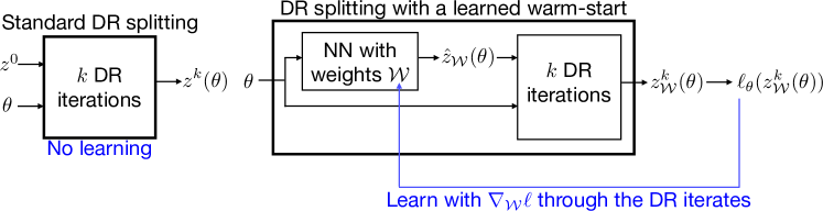
Figure 1: Left: standard DR splitting which maps parameter $\theta$ and initialization $z^{0}$ to an approximate solution $z^{k}(\theta)$. Right: Proposed learning framework consisting of two modules. The first module is the NN block which maps the parameter $\theta$ to a warm-start $\hat{z}_{\mathcal{W}}(\theta)$. The weights of the NN, denoted by $\mathcal{W}$, are the only variables we optimize over. The second module runs $k$ iterations of DR splitting (which also depend on $\theta$) starting with the warm-start $\hat{z}_{\mathcal{W}}(\theta)$ and returning a candidate solution $z^{k}_{\mathcal{W}}(\theta)$. We backpropagate from the loss $\ell_{\theta}(z^{k}_{\mathcal{W}}(\theta))$ through the DR iterates to learn the optimal weights $\mathcal{W}$.

• We propose a principled framework to learn high quality warm-starts from data. This framework consists of two modules as indicated in Figure 1. The first module is a feedforward neural network (NN) that predicts a warm-start from the problem parameters. The second module consists of $k$ DR splitting iterations that output the candidate solution. We differentiate the loss function with respect to the neural network weights by backpropagating through the DR iterates, which makes our framework an end-to-end warm-start learning scheme. Furthermore, our approach does not require us to solve optimization problems offline.

• We combine operator theory and Rademacher complexity theory to obtain novel generalization bounds that guarantee good performance for parametric QPs with unseen data. The bounds improve with the number of training problems and the number of DR iterations simultaneously, thereby allowing great flexibility in our learning task.

• We benchmark our approach on real-time quadratic optimization examples, showing that our method can produce an excellent warm-start that reduces the number of DR iterations required to reach a desired accuracy by at least $30\%$ and as much as $90\%$ in some cases.

2 Related work

Learning warm-starts.

A common approach to reduce the number of iterations of iterative algorithms is to learn a mapping from problem parameters to high-quality initializations. In optimal power flow, Baker (2019) trains a random forest to predict a warm-start. In the model predictive control (MPC) (Borrelli et al., 2017), Chen et al. (2022) use a neural network to accelerate the optimal control law computation by warm-starting an active set method. Other works in MPC use machine learning to predict an approximate optimal solution and, instead of using it to warm-start an algorithm, they directly ensure feasibility and optimality. Chen et al. (2018) and Karg and Lucia (2020) use a constrained neural network architecture that guarantees feasibility by projecting its output onto the QP feasible region. Zhang et al. (2019) uses a neural network to predict the solution while also certifying suboptimality of the output. In these works, the machine learning models do not consider that additional algorithmic steps will be performed after warm-starting. Our work differs in that the training of the NN is designed to minimize the loss after many steps of DR splitting. Additionally, our work is more general in scope since we consider general parametric QPs.

Learning algorithm steps.

There has been a wide array of works to speedup machine learning tasks by tuning algorithmic steps of stochastic gradient descent methods (Li and Malik, 2016; Andrychowicz et al., 2016; Metz et al., 2022; Chen et al., 2021; Amos, 2022). Similarly, Gregor and LeCun (2010) and Liu et al. (2019) accelerate the solution of sparse encoding problems by learning the step-size of the iterative soft thresholding algorithm. Operator splitting algorithms (Ryu and Yin, 2022) can also be speed up by learning acceleration steps (Venkataraman and Amos, 2021) or the closest contractive fixed-point iteration to achieve fast convergence (Bastianello et al., 2021). Reinforcement learning has also gained popularity as a versatile technique to accelerate the solution of parametric QPs by learning a policy to tune the step size of first-order methods (Ichnowski et al., 2021; Jung et al., 2022). A common tactic in these works is to differentiate through the steps of an algorithm to minimize a performance loss using gradient-based method. This known as loop unrolling which has been used in other areas such as meta-learning (Finn et al., 2017) and variational autoencoders (Kim et al., 2018). While we also unroll the algorithm iterations, our works differs in that we learn a high-quality warm-start rather than the algorithm steps. This allows us to guarantee convergence and also provide generalization bounds over the number of iterations.

Learning surrogates.

Instead of solving the original parametric problem, several works aim to learn a surrogate model that can be solved quickly in real-time applications. For example, by predicting which constraints are active (Misra et al., 2022) and the value of the optimal integer solutions (Bertsimas and Stellato, 2021, 2019) we can significantly accelerate the real-time solution of mixed-integer convex programs by solving, instead, a surrogate low-dimensional convex problem. Other approaches lean a mapping to reduce the dimensionality of the decision variables in the surrogate problem (Wang et al., 2020). This is achieved by embedding such problem as an implicit layer of a neural network and differentiating its KKT optimality conditions (Amos and Kolter, 2017; Amos et al., 2018; Agrawal et al., 2019). In contrast, our method does not approximate any problem and, instead, we predict a warm-start of the algorithmic procedure with a focus on real-time computations. This allows us to clearly quantify the suboptimality achieved within a fixed number of real-time iterations.

3 End-to-end learning framework

Problem formulation.

We consider the following parametric (convex) QP

$$\begin{array}[]{ll}\mbox{minimize}&(1/2)x^{T}Px+c^{T}x\\ \mbox{subject to}&Ax+s=b\\ &s\geq 0\end{array}\quad\text{ with parameter }\quad\theta=(\mathop{\bf vec{}}(P),\mathop{\bf vec{}}(A),c,b)\in{\mbox{\bf R}}^{d},$$ (1)

and decision variables $x\in\mathbf{R}^{n}$ and $s\in\mathbf{R}^{m}$. Here, $P$ is a positive semidefinite matrix in ${\mbox{\bf S}}_{+}^{n\times n}$, $A$ is a matrix in ${\mbox{\bf R}}^{m\times n}$, and $b$ and $c$ are vectors in ${\mbox{\bf R}}^{m}$ and ${\mbox{\bf R}}^{n}$ respectively. For a matrix $Y$, $\mathop{\bf vec{}}(Y)$ denotes the vector obtained by stacking the columns of $Y$. The dimension $d$ of $\theta$ is upper bounded by $mn+n^{2}+m+n$, but can be smaller in the case where only some of the data changes across the problems. Our goal is to quickly solve the QP in (1) with $\theta$ randomly drawn from a distribution $\mathcal{D}$ with compact support set $\Theta$, assuming that it admits an optimal solution for any $\theta\in\Theta$.

Optimality conditions.

The KKT optimality conditions of problem (1), that is, primal feasibility, dual feasibility, and complementary slackness, are given by

$$Ax+s=b,\quad A^{T}y+Px+c=0,\quad s\geq 0,\quad y\geq 0,\quad s\perp y=0,$$ (2)

where $y\in\mathbf{R}^{m}$ is the dual variable to problem (1). We can compactly write these conditions as a linear complementarity problem (O’Donoghue, 2021, Sec. 3), i.e., the problem of finding a $u=(x,y)\in{\mbox{\bf R}}^{m+n}$ such that

$$\mathcal{C}\ni u\perp Mu+q\in\mathcal{C}^{*},\quad\text{where}\quad M=\begin{bmatrix}P&A^{T}\\ -A&0\end{bmatrix}\in{\mbox{\bf R}}^{(m+n)\times(m+n)},$$ (3)

and $q=(c,b)\in{\mbox{\bf R}}^{m+n}$. Here, $\mathcal{C}={\mbox{\bf R}}^{n}\times{\mbox{\bf R}}_{+}^{m}$ and $\mathcal{C}^{*}=\{0\}^{n}\times\mathbf{R}_{+}^{m}$ denotes the dual cone to $\mathcal{C}$, i.e., $\mathcal{C}^{*}=\{w\mid w^{T}u\geq 0,\;u\in\mathcal{C}\}$. This problem is equivalent to finding $u\in{\mbox{\bf R}}^{m+m}$ that satisfies the following inclusion (Bauschke and Combettes, 2011, Ex. 26.22)(O’Donoghue, 2021, Sec. 3)

$$0\in Mu+q+N_{\mathcal{C}}(u),$$ (4)

where $N_{\mathcal{C}}(u)$ is the normal cone for cone $\mathcal{C}$ defined as $N_{\mathcal{C}}(z)=\{x\mid(y-u)^{T}x\leq 0,\forall y\in\mathcal{C}\}$ if $u\in\mathcal{C}$ and $\emptyset$ otherwise. Of importance to us to ensure convergence of the algorithm we define next is the fact that $Mu+q+N_{\mathcal{C}}(u)$ is maximal monotone; see (Ryu and Yin, 2022, Sec. 2.2) for a definition. This follows from $P\succeq 0$, $\mathcal{C}$ being a convex polyhedron, and (1) always admitting an optimal solution (Ryu and Yin, 2022, Thm. 7) (Ryu and Yin, 2022, Thm. 11).

Algorithm 1 The DR Splitting algorithm for $k$ iterations to solve problem (4).

Inputs: initial point $z^{0}$, problem data $(M,q)$, tolerance $\epsilon$, $k$ number of iterations
Output: approximate solution $z^{k}$
for $i=0,\dots,k-1$ do

       $u^{i+1}=\left(M+I\right)^{-1}\left(z^{i}-q\right)$
$\tilde{u}^{i+1}=\Pi_{\mathcal{C}}\left(2u^{i+1}-z^{i}\right)$
$z^{i+1}=z^{i}+\tilde{u}^{i+1}-u^{i+1}$

end for

Douglas-Rachford splitting.

We apply Douglas-Rachford (DR) splitting  (Lions and Mercier, 1979; Douglas and Rachford, 1956) to solve problem (4). DR consists of evaluating the resolvent of operators $Mu+q$ and $N_{\mathcal{C}}$, which for an operator $F$ is defined as $(I+F)^{-1}$ (Ryu and Yin, 2022, pp 40). By noting that the resolvent of $Mu+q$ is $(M+I)^{-1}(z-q)$ and the resolvent of $N_{\mathcal{C}}(u)$ is $\Pi_{\mathcal{C}}(z)$, i.e., the projection onto $\mathcal{C}$ (Ryu and Yin, 2022, Eq. 2.8, pp 42), we obtain Algorithm 1.

The linear system in the first step is always solvable since $M+I$ has full rank (O’Donoghue, 2021), but it varies from problem to problem. The projection onto $\mathcal{C}$, however, is the same for all problems and simply clips negative values to zero and leaves non-negative values unchanged. For compactness, in the remainder of the paper, we write Algorithm 1 as

$$z^{i+1}=T_{\theta}\left(z^{i}\right)\quad\text{where}\quad T_{\theta}(z)=z+\Pi_{\mathcal{C}}\left(2(M+I)^{-1}(z-q)-z\right)-(M+I)^{-1}(z-q).$$ (5)

We make the dependence of $T$ on $\theta$ explicit here as $M$ and $q$ are parametrized by $\theta$. DR splitting is guaranteed to converge to a fixed point $z^{\star}\in\mathop{\bf fix{}}T_{\theta}$ such that $T_{\theta}(z^{\star})=z^{\star}$. Algorithm 1 returns an approximate solution $z^{k}$, from which we can recover an approximate primal-dual solution to (1) by computing $(x^{k},y^{k})=u^{k}=(M+I)^{-1}(z^{k}-q)$ and $s^{k}=b-Ax^{k}$.

Our end-to-end learning architecture.

Our architecture consists of two modules as in Figure 1. The first module is a NN with weights $\mathcal{W}$: it predicts a good-quality initial point (or warm-start), $\hat{z}_{\mathcal{W}}(\theta)$, to Algorithm 1 from the parameter $\theta$ of the QP in (1). We assume that the NN has $L$ layers with ReLU activation functions (Ramachandran et al., 2017). We then write

$$\hat{z}_{\mathcal{W}}(\theta)=h_{\mathcal{W}}(\theta)=h_{L}\left(h_{L-1}\dots h_{1}(\theta)\right),$$

where $h_{l}(y_{l})=\left(W_{l}y_{l}+b_{l}\right)_{+}$, with $\{W_{l}\}_{l=0}^{L}$ being the weight matrices and $\{b_{l}\}_{l=0}^{L}$ the bias terms. Here, $h_{\mathcal{W}}(\cdot)$ is a mapping from ${\mbox{\bf R}}^{d}$ to ${\mbox{\bf R}}^{m+n}$ corresponding to the prediction and we denote the set of all such mappings by $\mathcal{H}$. We emphasize the dependency of $h$ on the weights and bias terms via the subscript $\mathcal{W}=(W_{1},b_{1},\dots,W_{L},b_{L})$. The second module corresponds to $k$ iterations of DR splitting from the initial point $\hat{z}_{\mathcal{W}}(\theta)$. It outputs an approximate solution $z^{k}_{\mathcal{W}}(\theta)$, from which we can recover an approximate solution to (1) as explained above. Using the operator in (5), we write

$$T^{k}_{\theta}(\hat{z}_{\mathcal{W}}(\theta))=z^{k}_{\mathcal{W}}(\theta).$$

To obtain the solution to a QP given parameter $\theta$, we simply need to perform a forward pass of the architecture, i.e., compute $T^{k}_{\theta}(h_{\mathcal{W}}(\theta))$, with $k$ chosen as needed.

Learning task.

We define the loss function as the fixed-point residual of operator $T_{\theta}$, i.e.,

$$\ell_{\theta}(z)=\|T_{\theta}(z)-z\|_{2}.$$ (6)

This loss measures the distance to convergence of Algorithm 1. The goal is to minimize the expected loss, which we define as the risk,

$$R(h_{\mathcal{W}})=\mathbf{E}_{\theta\sim\mathcal{D}}\left[\ell_{\theta}\left(T^{k}_{\theta}(h_{\mathcal{W}}(\theta))\right)\right],$$

with respect to the weights $\mathcal{W}$ of the NN. In general, we cannot evaluate $R(h_{\mathcal{W}})$ exactly and, instead, we minimize the empirical risk

$$\hat{R}(h_{\mathcal{W}})=(1/N)\sum_{i=1}^{N}\ell_{\theta_{i}}\left(T^{k}_{\theta_{i}}(h_{\mathcal{W}}(\theta_{i}))\right).$$ (7)

Here, $N$ is the number of training problems and we work with a full-batch approximation, though mini-batch or stochastic approximations can also be used (Sra et al., 2011).

Differentiability of our architecture.

To see that we can differentiate $\ell_{\theta}$ with respect to $\mathcal{W}$, note that the second module consists of repeated linear system solves and projections onto $\mathcal{C}$ (see Algorithm 1). Since the linear systems always have unique solutions, $u^{i+1}$ is linear in $z^{i}$ and the linear system solves are differentiable. Furthermore, as the projection step involves clipping non-negative values to zero, it is differentiable everywhere except at zero. In the first module, the NN consists entirely of differentiable functions except for the ReLU activation function, which is likewise differentiable everywhere except at zero.

4 Generalization bounds

In this section, we provide an upper bound on the expected loss $R(h_{\mathcal{W}})$ of our framework for any $h_{\mathcal{W}}\in\mathcal{H}$. This bound involves the empirical expected loss $\hat{R}(h_{\mathcal{W}})$, the Rademacher complexity of the NN appearing in the first module only and a term which decreases with both the number $k$ of iterations of DR splitting and the number $N$ of training samples. To obtain this bound, we rely on the fact that DR splitting on (4) achieves a linear convergence rate. More specifically, following (Banjac and Goulart, 2018, Thm. 1), we have that

$${\bf dist{}}_{\mathop{\bf fix{}}T_{\theta}}(T_{\theta}(z))\leq\beta_{\theta}{\bf dist{}}_{\mathop{\bf fix{}}T_{\theta}}(z)$$ (8)

where ${\bf dist{}}_{\mathcal{S}}(x)=\min\{||x-y||~{}|~{}y\in\mathcal{S}\}$ and $\beta_{\theta}\in(0,1)$ is the rate of linear convergence for problem with parameter $\theta$. We now state the result.

Theorem 1.

Let $\beta=\max_{\theta\in\Theta}\beta_{\theta}$ for $\beta_{\theta}$ as in (8). Assume that $\mathcal{H}$ is the set of mappings defined in Section 3 with the additional assumption that for any $h_{\mathcal{W}}\in\mathcal{H}$, ${\bf dist{}}_{\mathop{\bf fix{}}T_{\theta}}(h_{\mathcal{W}}(\theta))\leq B$ for some $B>0$ and any $\theta\in\Theta$. Then, with probability at least $1-\delta$ over the draw of i.i.d samples,

$$R(h_{\mathcal{W}})\leq\hat{R}(h_{\mathcal{W}})+2\sqrt{2}\beta^{k}\left(2{\bf rad}(\mathcal{H})+B\log(1/\delta)/(2N)\right),\quad\forall h_{\mathcal{W}}\in\mathcal{H},$$

where $k$ is the number of iterations of DR splitting in the second module, $N$ is the number of training samples, ${\bf rad}(\mathcal{H})$ is the Rademacher complexity of $\mathcal{H}$, and $\beta\in(0,1)$.

In settings where we can upper bound the Rademacher complexity of $\mathcal{H}$, for example in the case of NNs which are linear functions with bounded norm, or 2-layer NNs with ReLU activation functions, we are able to provide a bound on the generalization error of our framework which makes the dependence on $k$ and $N$ even more explicit (Golowich et al., 2018; Neyshabur et al., 2019).

Corollary 2.

Let $\mathcal{H}$ be the set of linear functions with bounded norm, i.e., $\mathcal{H}=\{h\mid h(\theta)=W\theta\}$ where $\theta\in{\mbox{\bf R}}^{d}$, $W\in{\mbox{\bf R}}^{(m+n)\times d}$ and $(1/2)||W||_{F}^{2}\leq B$ for some $B>0$. Then, with probability at least $1-\delta$ over the draw of i.i.d samples,

$$R(h_{\mathcal{W}})\leq\hat{R}(h_{\mathcal{W}})+2\sqrt{2}\beta^{k}\left(2\rho_{2}(\theta)\sqrt{2d/N}+B\log(1/\delta)/(2N)\right),\quad\forall h_{\mathcal{W}}\in\mathcal{H},$$

where $k$ and $N$ are as defined in Theorem 1, and $\rho_{2}(\theta)=\max_{\theta\in\Theta}||\theta||_{2}$ (Mohri et al., 2012, Thm. 5.10).

5 Numerical experiments

We now illustrate our method with examples of quadratic optimization problems deployed and repeatedly solved in control and portfolio optimization settings where rapid solutions are important for real-time execution and backtesting. Our architecture was implemented in the JAX library (Bradbury et al., 2018) with Adam (Kingma and Ba, 2015) training optimizer. All computations were run on the Princeton HPC Della Cluster. We use $10000$ training problems and evaluate on $2000$ test problems. In our examples we use a NN with three hidden layers of size $500$ each. Our code is available at https://github.com/stellatogrp/l2ws.

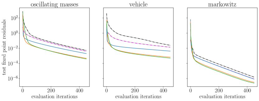
no warm-start   nearest neighbor warm-start   learned warm-start $k=${ $5$ $15$ $50$}

Figure 2: We plot the test fixed point residuals for different warm-starts of DR splitting. We train our architecture with $k=5,15,$ and $50$ DR iterations with loss function (7). We compare our results against a random initialization (black) and against warm-starting DR splitting with the nearest neighbor from the train set (magenta). Left: oscillating masses example. Middle: vehicle dynamics example. Right: portfolio optimization example.

5.1 Oscillating masses

We consider the problem of controlling a physical system that involves connected springs and masses (Wang and Boyd, 2010),(Chen et al., 2022, System 4). This can be formulated as the following QP:

$$\begin{array}[]{ll}\mbox{minimize}&x_{T}^{T}Q_{T}x_{T}+\sum_{t=1}^{T-1}x_{t}^{T}Qx_{t}+u_{t}^{T}Ru_{t}\\ \mbox{subject to}&x_{t+1}=Ax_{t}+Bu_{t}\quad t=0,\dots,T-1,\\ &u_{\textrm{min}}\leq u_{t}\leq u_{\textrm{max}}\quad t=0,\dots,T-1\\ &x_{\textrm{min}}\leq x_{t}\leq x_{\textrm{max}}\quad t=1,\dots,T,\\ &x_{0}=x_{\rm init}\\ \end{array}$$

where the states $x_{t}\in{\mbox{\bf R}}^{n}_{x}$ and the inputs $u_{t}\in{\mbox{\bf R}}^{n_{u}}$ are subject to lower and upper bounds. Matrices $A\in{\mbox{\bf R}}^{n_{x}\times n_{x}}$ and $B\in{\mbox{\bf R}}^{n_{x}\times n_{u}}$ define the system dynamics. The horizon length is $T$ and the parameter $\theta$ is initial state $x_{\rm init}$. Matrices $Q\in{\mbox{\bf S}}_{+}^{n_{x}}$ and $R\in{\mbox{\bf S}}_{++}^{n_{u}}$ define the state and input costs at each stage, and $Q_{T}\in{\mbox{\bf S}}_{+}^{n_{x}}$ the final stage cost.

Numerical example.

We consider $n_{x}=36$ states, $n_{u}=9$ control inputs, and a time horizon of $T=50$. Matrices $A$ and $B$ are obtained by discretizing the state dynamics with time step $0.5$ (Chen et al., 2022, System 4). We set $u_{\textrm{min}}=-u_{\textrm{max}}=1/2$ and $x_{\textrm{min}}=-x_{\textrm{max}}=2$. We set $Q_{t}=I$ for $t=1,\dots,T$, and $R_{t}=I$ for $t=1,\dots,T-1$. We sample $\theta=x_{\rm init}$ uniformly in $[-2,2]^{36}$. Figure 2 and Table 5.1 show the convergence behavior of our method.

Table 1: Oscillating masses problem. We compare the number of iterations of DR splitting required to reach different levels of accuracy with different warm-starts (learned warm-start with $k=5,15,50$, no warm-start, and a nearest neighbor warm-start). The reduction columns are the iterations reduced as a fraction of the no learning iterations.

	no learning	nearest neighbor		train $k=5$		train $k=15$		train $k=50$
$\epsilon$	iters	iters	reduction	iters	reduction	iters	reduction	iters	reduction
[head to column names, late after line=

5.2 Vehicle dynamics control problem

We consider problem of controlling a vehicle, modeled as a parameter-varying linear dynamical system (Takano et al., 2003), to track a reference trajectory (Zhang et al., 2019). We formulate it as the following QP

$$\begin{array}[]{ll}\mbox{minimize}&(y_{T}-y_{T}^{\textrm{ref}})^{T}Q(y_{T}-y_{T}^{\textrm{ref}})+\sum_{t=1}^{T-1}(y_{t}-y_{t}^{\textrm{ref}})^{T}Q_{T}(y_{t}-y_{t}^{\textrm{ref}})+u_{t}^{T}Ru_{t}\\ \mbox{subject to}&x_{t+1}=A(v)x_{t}+B(v)u_{t}+E(v)\delta_{t}\quad t=0,\dots,T-1\\ &|u_{t}|\leq\bar{u},\quad|u_{t}-u_{t-1}|\leq\overline{\Delta u},\quad t=0,\dots,T-1\\ &y_{t}=Cx_{t},\quad t=0,\dots,T-1\\ &x_{0}=x_{\rm init},\end{array}$$

where $x_{t}\in{\mbox{\bf R}}^{4}$ is the state and $u_{t}\in{\mbox{\bf R}}^{3}$ is the input, and $\delta_{t}\in{\mbox{\bf R}}$ is the driver steering input, which we assume is linear over time. We aim to minimize the distance between the output, $y_{t}\in{\mbox{\bf R}}^{3}$ and the reference trajectory $y_{t}^{\textrm{ref}}\in{\mbox{\bf R}}^{3}$ over time. Matrices $Q\in{\mbox{\bf S}}_{+}^{n_{x}}$ and $Q_{T}\in{\mbox{\bf S}}_{+}^{n_{x}}$ define the state costs, $R\in{\mbox{\bf S}}_{++}^{n_{u}}$ the input cost, and $C\in{\mbox{\bf R}}^{3\times 4}$ the output $y_{t}$. The term $v\in{\mbox{\bf R}}$ is the longitudinal velocity of the vehicle that parametrizes $A\in{\mbox{\bf R}}^{4\times 4},B\in{\mbox{\bf R}}^{4\times 3}$, and $E\in{\mbox{\bf R}}^{4}$. Vectors $\bar{u}$ and $\overline{\Delta u}$ bound the magnitude of the inputs and change in inputs respectively. The parameters $\theta$ for the problem are the initial state $x_{\rm init}$, the initial velocity $v$, the previous control input $u_{-1}$, the reference signals $y_{t}^{\rm ref}$ for $t=0,\dots,T$, and the steering inputs $\delta_{t}$ for $t=0,\dots,T-1$.

Numerical example.

The time horizon is $T=30$. Matrices $A,B,E$ result from discretizing the dynamics (Takano et al., 2003). We sample all parameters uniformly from their bounds: the velocity $v\in[2,35]$, the output $y_{t}\in[-\bar{y},\bar{y}]$ where $\bar{y}=(25,40,30)$ in degrees, and the previous control $u_{-1}\in[-\bar{u},\bar{u}]$ where $\bar{u}=10^{3}(1,20,30)$. We sample the initial steering angle from $[-45,45]$ and its linear increments from $[-30,30]$. Figure 2 and Table 5.2 show the performance of our method.

Table 2: Vehicle problem. We compare the number of iterations of DR splitting required to reach different levels of accuracy with different warm-starts (learned warm-start with $k=5,15,50$, no warm-start, and a nearest neighbor warm-start). The reduction columns are the iterations reduced as a fraction of the no learning iterations.

	no learning	nearest neighbor		train $k=5$		train $k=15$		train $k=50$
$\epsilon$	iters	iters	reduction	iters	reduction	iters	reduction	iters	reduction
[head to column names, late after line=

5.3 Portfolio optimization

We consider the portfolio optimization problem where we want to allocate assets to maximize the risk-adjusted return (Markowitz, 1952; Boyd et al., 2017),

$$\begin{array}[]{ll}\mbox{maximize}&\rho\mu^{T}x-x^{T}\Sigma x\\ \mbox{subject to}&\mathbf{1}^{T}x=1,\quad x\geq 0,\end{array}$$

where $x\in{\mbox{\bf R}}^{n}$ represents the portfolio, $\mu\in{\mbox{\bf R}}^{n}$ the expected returns, $1/\rho>0$ the risk-aversion parameter, and $\Sigma\in{\mbox{\bf S}}_{+}^{n}$ the return covariance. For this problem, $\theta=\mu$.

Numerical example.

We use real-world stock return data from $3000$ popular assets from 2015-2019 (Nasdaq, 2022). We use an $l$-factor model for the risk and set $\Sigma=F\Sigma_{F}F^{T}+D$ where $F\in{\mbox{\bf R}}^{n,l}$ is the factor-loading matrix, $\Sigma_{F}\in{\mbox{\bf S}}_{+}^{l}$ estimates the factor returns, and $D\in{\mbox{\bf S}}_{+}^{n}$ is a diagoal matrix accounting for additional variance for each asset also called the idiosyncratic risk. We compute the factor model with $15$ factors by using the same approach as in (Boyd et al., 2017). The return parameters are $\mu=\alpha(\hat{\mu_{t}}+\epsilon_{t})$ where $\hat{\mu_{t}}$ is the realized return at time $t$, $\epsilon_{t}\sim\mathcal{N}(0,\sigma_{\epsilon}I)$, and $\alpha=0.24$ is selected to minimize the mean squared error $\mathbf{E}\|\mu_{t}-\hat{\mu}_{t}\|_{2}^{2}$ (Boyd et al., 2017). We iterate and repeatedly cycle over the five year period to sample a $\mu$ vector for each of our problems. Figure 2 and Table 5.3 show the performance of our method.

Table 3: Markowitz problem. We compare the number of iterations of DR splitting required to reach different levels of accuracy with different warm-starts (learned warm-start with $k=5,15,50$, no warm-start, and a nearest neighbor warm-start). The reduction columns are the iterations reduced as a fraction of the no learning iterations.

	no learning	nearest neighbor		train $k=5$		train $k=15$		train $k=50$
$\epsilon$	iters	iters	reduction	iters	reduction	iters	reduction	iters	reduction
[head to column names, late after line=

Appendix A Proof of the generalization bound

A.1 Proof of Theorem 1

For ease of notation, let $s(\theta)=\ell_{\theta}\left(T^{k}_{\theta}(h_{\mathcal{W}}(\theta))\right)$. The function class we consider is $\mathcal{S}=\{s\mid s(\theta)=\ell_{\theta}\left(T^{k}_{\theta}(h_{\mathcal{W}}(\theta))\right),h_{\mathcal{W}}\in\mathcal{H}\}$. The risk and empirical risk for $s$ are $R(s)=\mathbf{E}[s(\theta)]$ and $\hat{R}(s)=(1/N)\sum_{i=1}^{N}s(\theta_{i})$, respectively. Assume that the loss is bounded over all $s\in\mathcal{S}$ and $\theta\in\Theta$, $s(\theta)\leq b$. Note that $\hat{R}(s)=R(h_{\mathcal{W}})$ and $R(s)=\hat{R}(h_{\mathcal{W}})$. For any $\delta>0$, with probability at least $1-\delta$ over the draw of an i.i.d. sample $S$ of size $N$, each of the following holds  (Bartlett and Mendelson, 2002)(Mohri et al., 2012, Thm. 3.3):

$$R(h_{\mathcal{W}})\leq\hat{R}(h_{\mathcal{W}})+2{\bf rad}_{S}(\mathcal{S})+b\sqrt{\log 1/\delta/(2N)},$$ (9)

for all $h_{\mathcal{W}}\in\mathcal{H}.$ To prove Theorem 1, we need to bound ${\bf rad}_{S}(\mathcal{S})$ and $b$.

Lemma 3.

Let $T_{\theta}$ satisfy equation (8). Take $\beta=\max_{\theta\in\Theta}\beta_{\theta}$. Then,

$$\ell_{\theta}(T^{k}_{\theta}(z))\leq 2\beta^{k}{\bf dist{}}_{\mathop{\bf fix{}}T_{\theta}}(z)\quad\forall\theta\in\Theta.$$ (10)

Proof.

From the definition of the loss $\ell_{\theta}$ in (6), for any $w\in\mathop{\bf fix{}}T_{\theta}$ we have

$$\ell_{\theta}(T^{k}_{\theta}(z)) =\|T^{k+1}_{\theta}(z)-T^{k}_{\theta}(z)\|_{2}\leq\|T^{k}_{\theta}(z)-w\|_{2}+\|T^{k+1}_{\theta}(z)-w\|_{2}$$

$$\leq\|T^{k}_{\theta}(z)-w\|_{2}+\|T^{k}_{\theta}(z)-w\|_{2}\leq 2{\bf dist{}}_{\mathop{\bf fix{}}T_{\theta}}(T^{k}_{\theta}(z))\leq 2\beta^{k}{\bf dist{}}_{\mathop{\bf fix{}}T_{\theta}}(z),$$

where the first inequality comes from the triangle inequality, the second-inequality from $w\in\mathop{\bf fix{}}T_{\theta}$ and non-expansiveness of $T_{\theta}$, and the last inequality from the definition of ${\bf dist{}}_{\mathop{\bf fix{}}T_{\theta}}$. ∎

Lemma 4.

Assume that $\forall\theta\in\Theta$, $\mathcal{H}\subseteq\{h_{\mathcal{W}}\mid{\bf dist{}}_{\mathop{\bf fix{}}T_{\theta}}(h_{\mathcal{W}}(\theta))\leq B\}$ and that $T_{\theta}$ satisfies equation (8) with parameter $\beta$. Let $\epsilon$ and $\epsilon_{j}$ be i.i.d. Rademacher random variables. Then,

$$\textstyle\mathop{\bf E{}}\left[\sup_{h_{\mathcal{W}}\in\mathcal{H}}\epsilon\ell_{\theta}\left(T^{k}_{\theta}(h_{\mathcal{W}}(\theta))\right)\right]\leq 2\sqrt{2}\beta^{k}\mathbf{E}\left[\sup_{h_{\mathcal{W}}\in\mathcal{H}}\sum_{j}\epsilon_{j}h_{\mathcal{W}}(z_{j})\right].$$ (11)

Proof.

Denote $Z_{\theta}$ to be the set of possible predictions of $\mathcal{H}$ for a fixed $\theta$. That is, $Z_{\theta}=\{h_{\mathcal{W}}(\theta)\mid h_{\mathcal{W}}\in\mathcal{H}\}$. Let $\bar{z}_{\theta}=\operatorname*{arg\,max}_{z\in Z_{\theta}}\ell_{\theta}(T^{k}_{\theta}(\theta)))$.

$$\textstyle 2\mathbf{E}\left[\sup_{h_{\mathcal{W}}\in\mathcal{H}}\epsilon\ell_{\theta}\left(T^{k}_{\theta}(h_{\mathcal{W}}(\theta))\right)\right] =\textstyle 2\mathbf{E}\left[\sup_{z\in Z_{\theta}}\epsilon\ell_{\theta}\left(T^{k}_{\theta}(z)\right)\right]$$

$$\textstyle=\sup_{z,w\in Z_{\theta}}\ell_{\theta}\left(T^{k}_{\theta}(z)\right)-\ell_{\theta}\left(T^{k}_{\theta}(w)\right)=\ell_{\theta}\left(T^{k}_{\theta}(\bar{z}_{\theta})\right)$$

$$\textstyle\leq 2\beta^{k}{\bf dist{}}_{\mathop{\bf fix{}}T_{\theta}}(\bar{z}_{\theta})\leq 2\beta^{k}\|\bar{z}_{\theta}-\tilde{z}_{\theta}\|_{2}$$

$$\textstyle\leq 2\sqrt{2}\beta^{k}\mathbf{E}\left[\left\lvert\sum_{j}\epsilon_{j}(\bar{z}_{\theta}-\tilde{z}_{\theta})_{j}\right\rvert\right]$$

$$\textstyle\leq 2\sqrt{2}\beta^{k}\mathbf{E}\left[\left\lvert\sup_{z,w\in Z_{\theta}}\sum_{k}\epsilon_{j}z_{j}-\sum_{j}\epsilon_{j}w_{j}\right\rvert\right]$$

$$\textstyle=2\sqrt{2}\beta^{k}\left(\mathbf{E}\left[\sup_{z\in Z_{\theta}}\sum_{j}\epsilon_{j}z_{j}\right]+\mathbf{E}\left[\sup_{w\in h_{\mathcal{W}}(\theta)}\sum_{j}-\epsilon_{j}w_{j}\right]\right)$$

$$\textstyle=4\sqrt{2}\beta^{k}\mathbf{E}\left[\sup_{h_{\mathcal{W}}\in\mathcal{H}}\sum_{j}\epsilon_{j}h_{\mathcal{W}}(z_{j})\right]$$

The second line uses the definition of the Rademacher random variable. The supremum of the difference is achieved by maximizing $\ell_{\theta}\left(T^{k}_{\theta}(z)\right)$ for $z$ and picking $w\in\mathop{\bf fix{}}T_{\theta}$. The third line uses Lemma 3 and we pick any fixed point, $\tilde{z}_{\theta}\in\mathop{\bf fix{}}_{T_{\theta}}$. The fourth line uses (Maurer, 2016, Prop. 6). The fifth line follows from replacing $\bar{z}_{\theta}$ and $\tilde{z}_{\theta}$ with a supremum over $Z_{\theta}$. In second to last line we remove the absolute value because the same maximum will be attained by maximizing the difference. The last line comes from the symmetry of the Rademacher random variable. ∎

To get the final result, we use (Maurer, 2016, Thm. 3) which involved a induction step to sum over the $N$ samples and Lemma 4. Then, (Maurer, 2016, Cor. 4) directly follows and we finish with

$$\textstyle{\bf erad}_{S}(\mathcal{S}) \textstyle=\mathop{\bf E{}}_{\sigma}\left[\sup_{h_{\mathcal{W}}\in\mathcal{H}}\frac{1}{N}\sum_{i=1}^{N}\sigma_{i}\ell_{\theta_{i}}\left(T^{k}_{\theta_{i}}(h_{\mathcal{W}}(\theta_{i}))\right)\right]$$

$$\textstyle\leq 2\sqrt{2}\beta^{k}\mathop{\bf E{}}_{\sigma}\left[\sup_{h_{\mathcal{W}}\in\mathcal{H}}\frac{1}{N}\sum_{i=1}^{N}\sigma_{i}^{T}h_{\mathcal{W}}(\theta_{i})\right]$$

$$\textstyle=2\sqrt{2}\beta^{k}{\bf erad}_{S}(\mathcal{H}).$$

The empirical Rademacher complexity of $\mathcal{S}$ over samples $S$ is ${\bf erad}_{S}(\mathcal{S})$. The inequality comes from Lemma 4. The last line follows from the definition of the multivariate empirical Rademacher complexity of $\mathcal{H}$. The worst-case loss is $2\beta^{k}B$ which follows from Lemma 3. Last, we take the expectation to get the same bound for the Rademacher complexity and use Equation (9) to finish the proof.

Acknowledgments

The author(s) are pleased to acknowledge that the work reported on in this paper was substantially performed using the Princeton Research Computing resources at Princeton University which is consortium of groups led by the Princeton Institute for Computational Science and Engineering (PICSciE) and Office of Information Technology’s Research Computing.

References

- Agrawal et al. (2019) A. Agrawal, S. Barratt, S. Boyd, E. Busseti, and W. Moursi. Differentiating through a cone program. Journal of Applied and Numerical Optimization, 1(2):107–115, 2019.
- Amos (2022) B. Amos. Tutorial on amortized optimization for learning to optimize over continuous domains, 2022. URL https://arxiv.org/abs/2202.00665.
- Amos and Kolter (2017) B. Amos and Z. Kolter. Optnet: Differentiable optimization as a layer in neural networks. In D. Precup and Y. W. Teh, editors, Proceedings of the 34th International Conference on Machine Learning, volume 70 of Proceedings of Machine Learning Research, pages 136–145, International Convention Centre, Sydney, Australia, 06–11 Aug 2017. PMLR. URL http://proceedings.mlr.press/v70/amos17a.html.
- Amos et al. (2018) B. Amos, I. D. J. Rodriguez, J. Sacks, B. Boots, and J. Z. Kolter. Differentiable mpc for end-to-end planning and control. arXiv preprint arXiv:1810.13400, 2018.
- Andrychowicz et al. (2016) M. Andrychowicz, M. Denil, S. G. Colmenarejo, M. W. Hoffman, D. Pfau, T. Schaul, B. Shillingford, and N. de Freitas. Learning to learn by gradient descent by gradient descent. In Proceedings of the 30th International Conference on Neural Information Processing Systems, NIPS’16, page 3988–3996, Red Hook, NY, USA, 2016. Curran Associates Inc. ISBN 9781510838819.
- Baker (2019) K. Baker. Learning warm-start points for ac optimal power flow. In 2019 IEEE 29th International Workshop on Machine Learning for Signal Processing (MLSP), pages 1–6, 2019. doi: 10.1109/MLSP.2019.8918690.
- Banjac and Goulart (2018) G. Banjac and P. J. Goulart. Tight global linear convergence rate bounds for operator splitting methods. IEEE Transactions on Automatic Control, 63(12):4126–4139, 2018. doi: 10.1109/TAC.2018.2808442.
- Bartlett and Mendelson (2002) P. L. Bartlett and S. Mendelson. Rademacher and gaussian complexities: Risk bounds and structural results. J. Mach. Learn. Res., 3:463–482, 2002. URL http://dblp.uni-trier.de/db/journals/jmlr/jmlr3.html#BartlettM02.
- Bastianello et al. (2021) N. Bastianello, A. Simonetto, and E. Dall’Anese. Opreg-boost: Learning to accelerate online algorithms with operator regression, 2021. URL https://arxiv.org/abs/2105.13271.
- Bauschke and Combettes (2011) H. H. Bauschke and P. L. Combettes. Convex Analysis and Monotone Operator Theory in Hilbert Spaces. Springer, 1st edition, 2011.
- Beck (2017) A. Beck. First-Order Methods in Optimization. Society for Industrial and Applied Mathematics, Philadelphia, PA, 2017. doi: 10.1137/1.9781611974997. URL https://epubs.siam.org/doi/abs/10.1137/1.9781611974997.
- Bertsimas and Stellato (2019) D. Bertsimas and B. Stellato. Online mixed-integer optimization in milliseconds. arXiv e-prints, July 2019. URL https://arxiv.org/abs/1907.02206.
- Bertsimas and Stellato (2021) D. Bertsimas and B. Stellato. The voice of optimization. Machine Learning, 110:249–277, Feb 2021. URL https://doi.org/10.1007/s10994-020-05893-5.
- Borrelli et al. (2017) F. Borrelli, A. Bemporad, and M. Morari. Predictive Control for Linear and Hybrid Systems. Cambridge University Press, 2017. doi: 10.1017/9781139061759.
- Boyd et al. (2017) S. Boyd, E. Busseti, S. Diamond, R. N. Kahn, K. Koh, P. Nystrup, and J. Speth. Multi-period trading via convex optimization, 2017. URL https://arxiv.org/abs/1705.00109.
- Boyd et al. (2011) S. P. Boyd, N. Parikh, E. K. wah Chu, B. Peleato, and J. Eckstein. Distributed optimization and statistical learning via the alternating direction method of multipliers. Found. Trends Mach. Learn., 3:1–122, 2011.
- Bradbury et al. (2018) J. Bradbury, R. Frostig, P. Hawkins, M. J. Johnson, C. Leary, D. Maclaurin, G. Necula, A. Paszke, J. VanderPlas, S. Wanderman-Milne, and Q. Zhang. JAX: composable transformations of Python+NumPy programs, 2018. URL http://github.com/google/jax.
- Chen et al. (2018) S. Chen, K. Saulnier, N. Atanasov, D. D. Lee, V. Kumar, G. J. Pappas, and M. Morari. Approximating explicit model predictive control using constrained neural networks. In 2018 Annual American Control Conference (ACC), pages 1520–1527, 2018. doi: 10.23919/ACC.2018.8431275.
- Chen et al. (2022) S. W. Chen, T. Wang, N. Atanasov, V. Kumar, and M. Morari. Large scale model predictive control with neural networks and primal active sets. Automatica, 135:109947, 2022. ISSN 0005-1098. doi: https://doi.org/10.1016/j.automatica.2021.109947. URL https://www.sciencedirect.com/science/article/pii/S0005109821004738.
- Chen et al. (2021) T. Chen, X. Chen, W. Chen, H. Heaton, J. Liu, Z. Wang, and W. Yin. Learning to optimize: A primer and a benchmark, 2021. URL https://arxiv.org/abs/2103.12828.
- Douglas and Rachford (1956) J. Douglas and H. H. Rachford. On the numerical solution of heat conduction problems in two and three space variables. Transactions of the American Mathematical Society, 82(2):421–439, 1956. ISSN 00029947. URL http://www.jstor.org/stable/1993056.
- Ferreau et al. (2014) H. J. Ferreau, C. Kirches, A. Potschka, H. G. Bock, and M. Diehl. qpoases: a parametric active-set algorithm for quadratic programming. Mathematical Programming Computation, 6:327–363, 2014.
- Finn et al. (2017) C. Finn, P. Abbeel, and S. Levine. Model-agnostic meta-learning for fast adaptation of deep networks. In D. Precup and Y. W. Teh, editors, Proceedings of the 34th International Conference on Machine Learning, volume 70 of Proceedings of Machine Learning Research, pages 1126–1135. PMLR, 06–11 Aug 2017. URL https://proceedings.mlr.press/v70/finn17a.html.
- Golowich et al. (2018) N. Golowich, A. Rakhlin, and O. Shamir. Size-independent sample complexity of neural networks. In S. Bubeck, V. Perchet, and P. Rigollet, editors, Proceedings of the 31st Conference On Learning Theory, volume 75 of Proceedings of Machine Learning Research, pages 297–299. PMLR, 06–09 Jul 2018.
- Gregor and LeCun (2010) K. Gregor and Y. LeCun. Learning fast approximations of sparse coding. In Proceedings of the 27th International Conference on International Conference on Machine Learning, ICML’10, page 399–406, Madison, WI, USA, 2010. Omnipress. ISBN 9781605589077.
- Ichnowski et al. (2021) J. Ichnowski, P. Jain, B. Stellato, G. Banjac, M. Luo, F. Borrelli, J. E. Gonzales, I. Stoica, and K. Goldberg. Accelerating quadratic optimization with reinforcement learning. In Advances in Neural Information Processing Systems 35, 12 2021. URL https://arxiv.org/pdf/2107.10847.pdf.
- Jung et al. (2022) H. Jung, J. Park, and J. Park. Learning context-aware adaptive solvers to accelerate quadratic programming, 2022. URL https://arxiv.org/abs/2211.12443.
- Karg and Lucia (2020) B. Karg and S. Lucia. Efficient representation and approximation of model predictive control laws via deep learning. IEEE Transactions on Cybernetics, PP:1–13, 06 2020. doi: 10.1109/TCYB.2020.2999556.
- Kim et al. (2018) Y. Kim, S. Wiseman, A. Miller, D. Sontag, and A. Rush. Semi-amortized variational autoencoders. In J. Dy and A. Krause, editors, Proceedings of the 35th International Conference on Machine Learning, volume 80 of Proceedings of Machine Learning Research, pages 2678–2687. PMLR, 10–15 Jul 2018. URL https://proceedings.mlr.press/v80/kim18e.html.
- Kingma and Ba (2015) D. P. Kingma and J. Ba. Adam: A method for stochastic optimization. In Y. Bengio and Y. LeCun, editors, 3rd International Conference on Learning Representations, ICLR 2015, San Diego, CA, USA, May 7-9, 2015, Conference Track Proceedings, 2015. URL http://arxiv.org/abs/1412.6980.
- Kuindersma et al. (2014) S. Kuindersma, F. Permenter, and R. Tedrake. An efficiently solvable quadratic program for stabilizing dynamic locomotion. 06 2014. doi: 10.1109/ICRA.2014.6907230.
- Li and Malik (2016) K. Li and J. Malik. Learning to optimize, 2016. URL https://arxiv.org/abs/1606.01885.
- Lions and Mercier (1979) P. L. Lions and B. Mercier. Splitting algorithms for the sum of two nonlinear operators. SIAM Journal on Numerical Analysis, 16(6):964–979, 1979. doi: 10.1137/0716071. URL https://doi.org/10.1137/0716071.
- Liu et al. (2019) J. Liu, X. Chen, Z. Wang, and W. Yin. ALISTA: Analytic weights are as good as learned weights in LISTA. In International Conference on Learning Representations, 2019. URL https://openreview.net/forum?id=B1lnzn0ctQ.
- Markowitz (1952) H. Markowitz. Portfolio selection. The Journal of Finance, 7(1):77–91, 1952. ISSN 00221082, 15406261. URL http://www.jstor.org/stable/2975974.
- Maurer (2016) A. Maurer. A vector-contraction inequality for rademacher complexities. In R. Ortner, H. U. Simon, and S. Zilles, editors, Algorithmic Learning Theory, pages 3–17, Cham, 2016. Springer International Publishing. ISBN 978-3-319-46379-7.
- Metz et al. (2022) L. Metz, J. Harrison, C. D. Freeman, A. Merchant, L. Beyer, J. Bradbury, N. Agrawal, B. Poole, I. Mordatch, A. Roberts, and J. Sohl-Dickstein. Velo: Training versatile learned optimizers by scaling up, 2022. URL https://arxiv.org/abs/2211.09760.
- Misra et al. (2022) S. Misra, L. Roald, and Y. Ng. Learning for constrained optimization: Identifying optimal active constraint sets. INFORMS J. on Computing, 34(1):463–480, jan 2022. ISSN 1526-5528. doi: 10.1287/ijoc.2020.1037. URL https://doi.org/10.1287/ijoc.2020.1037.
- Mohri et al. (2012) M. Mohri, A. Rostamizadeh, and A. S. Talwalkar. Foundations of machine learning. In Adaptive computation and machine learning, 2012.
- Nasdaq (2022) Nasdaq. End-of-day us stock prices. https://data.nasdaq.com/databases/EOD/documentation, 2022. This data was obtained and used solely by Princeton University.
- Neyshabur et al. (2019) B. Neyshabur, Z. Li, S. Bhojanapalli, Y. LeCun, and N. Srebro. The role of over-parametrization in generalization of neural networks. In International Conference on Learning Representations, 2019. URL https://openreview.net/forum?id=BygfghAcYX.
- O’Donoghue (2021) B. O’Donoghue. Operator splitting for a homogeneous embedding of the linear complementarity problem. SIAM Journal on Optimization, 31(3):1999–2023, 2021. doi: 10.1137/20M1366307. URL https://doi.org/10.1137/20M1366307.
- Ramachandran et al. (2017) P. Ramachandran, B. Zoph, and Q. V. Le. Swish: a self-gated activation function. arXiv: Neural and Evolutionary Computing, 2017.
- Ryu and Yin (2022) E. K. Ryu and W. Yin. Large-Scale Convex Optimization: Algorithms amp; Analyses via Monotone Operators. Cambridge University Press, 2022.
- Sra et al. (2011) S. Sra, S. Nowozin, and S. J. Wright. Optimization for Machine Learning. The MIT Press, 2011. ISBN 026201646X.
- Stellato et al. (2020) B. Stellato, G. Banjac, P. Goulart, A. Bemporad, and B. Stephen. OSQP: An Operator Splitting Solver for Quadratic Programs. Mathematical Programming Computation, 12(4):637–672, 10 2020. URL https://doi.org/10.1007/s12532-020-00179-2.
- Takano et al. (2003) S. Takano, M. Nagai, T. Taniguchi, and T. Hatano. Study on a vehicle dynamics model for improving roll stability. JSAE Review, 24(2):149–156, 2003. ISSN 0389-4304. doi: https://doi.org/10.1016/S0389-4304(03)00012-2. URL https://www.sciencedirect.com/science/article/pii/S0389430403000122.
- Venkataraman and Amos (2021) S. Venkataraman and B. Amos. Neural fixed-point acceleration for convex optimization. CoRR, abs/2107.10254, 2021. URL https://arxiv.org/abs/2107.10254.
- Wang et al. (2020) K. Wang, B. Wilder, A. Perrault, and M. Tambe. Automatically learning compact quality-aware surrogates for optimization problems. In Proceedings of the 34th International Conference on Neural Information Processing Systems, NIPS’20, Red Hook, NY, USA, 2020. Curran Associates Inc. ISBN 9781713829546.
- Wang and Boyd (2010) Y. Wang and S. Boyd. Fast model predictive control using online optimization. IEEE Transactions on Control Systems Technology, 18(2):267–278, 2010. doi: 10.1109/TCST.2009.2017934.
- Zhang et al. (2019) X. Zhang, M. Bujarbaruah, and F. Borrelli. Safe and near-optimal policy learning for model predictive control using primal-dual neural networks. In 2019 American Control Conference (ACC), pages 354–359, 2019. doi: 10.23919/ACC.2019.8814335.