Towards Robust Calculation of index-$k$ Saddle Point: Iterative Proximal-Minimization and Differential Game Model

Abstract

Saddle point with a given Morse index on a potential energy surface is an important object related to energy landscape in physics and chemistry. Efficient numerical methods based on iterative minimization formulation have been proposed in the forms of the sequence of minimization subproblems or the continuous dynamics. We here present a differential game interpretation of this formulation and theoretically investigate the Nash equilibrium of the proposed game and the original saddle point on potential energy surface. To define this differential game, a new proximal function growing faster than quadratic is introduced to the cost function in the game and a robust Iterative Proximal-Minimization algorithm (IPM) is then derived to compute the saddle points. We prove that the Nash equilibrium of the game is exactly the saddle point in concern and show that the new algorithm is more robust than the previous iterative minimization algorithm without proximity, while the same convergence rate and the computational cost still hold. A two dimensional problem and the Cahn-Hillard problem are tested to demonstrate this numerical advantage.

68Q25, 68R10, 68U05

1 Introduction

Saddle points with important physical meaning have been of broad interest in physics, chemistry, biology and material sciences[31]. In computational chemistry, besides multiple local minimum points, one of the most important objects on the potential energy surface is the transition state. Such transition states are the bottlenecks on the most probable transition paths between different local wells[4, 2, 8]. In general, the transition state can be described as a special type of the saddle point with Morse index 1, which is defined as the critical point with only one unstable direction.

In recent years, a large number of numerical methods have been proposed [8, 19, 18, 10, 11, 34, 36] and developed [9, 28, 17, 12, 35] to efficiently compute these index-1 saddle points. Most of them [10, 11, 33] can be generalized to the case with the Morse index $k\geq 1$. In addition, for applications to multiple unstable solutions of certain nonlinear partial differential equations, there are computational methods based on mountain pass and local min-max method [5, 24, 32] which however do not aim for specific index.

One important class of algorithms for saddle points with a given index is based on the idea of using the min-mode direction[6, 18, 10, 34, 11, 35, 29]. The work of the iterative minimization formulation (IMF) [11] builds a rigorous mathematical model for this min-mode idea and then a series of IMF-based algorithms have been developed[20, 12, 14], generalized[15, 17] and analyzed [22]. Although the IMF enjoys the quadratic convergence rate[11], the convergence is only local and is subject to the quality of the initial conditions. However, in practice, this problem can be much alleviated by using adaptive inexact solver[10, 12] for the sub-problems in the IMF. In most cases, such a trade-off between efficiency and robustness works well for applications of these algorithms, but this demands a careful tuning of parameters and a brute-force randomized strategy. On the other side, the continuous model of the IMF as the one-step approximation to the subproblems, which is called gentlest ascent dynamics (GAD) [10], is empirically found to be more robust [12, 23] than the vanilla IMF, but GAD only has a linear convergence speed. These current research results thus require a further exploration of the underlying reasons of the numerical divergence issue. We believe this issue at least partially comes from the lack of convexity in the sub-problem of optimizing an auxiliary function in the IMF. To investigate this practical challenge, we take a new viewpoint of game theory and its connection to the saddle point.

The IMF defines an iterative scheme for both a position variable and an orientation vector, whose fixed point, if converged, is an index-1 saddle point. At this fixed point, the position variable and the orientation variable minimize their own objective functions, respectively. This form is very much like a differential game model [1], where the central notion is the Nash equilibrium in game theory [25]. Our main work here is to explicitly investigate such connections between the existing IMF algorithms and differential game models. We shall see that for a differential game well defined compatible with the IMF, one needs to improve the existing auxiliary function used in the original IMF. Our main technique is to introduce a proximal function as a penalty to the existing auxiliary function to ensure its strict convexity. We show that one has to choose the proximal function growing faster than quadratic function, in contrast to the squared $L_{2}$ norm in classic proximal point algorithms. With this new proximal technique, we construct a new method, called Iterative Proximal Minimization (IPM) method, as an important improvement of the existing IMF-based algorithms. In theory, we contribute to the proof of the equivalence between the following three objects: saddle point of the potential function, the fixed point of the new iterative scheme, and the Nash equilibrium of the differential game.

The new strategy of using a proper proximal function as a penalty in this proposed iterative proximal minimization method is very easy to implement without any extra computational burden than the existing methods. The quadratic convergence rate still preserves. Most importantly, the new iterative proximal method can significantly enhance the robustness since each subproblem has a well-defined minimizer. Extensive numerical experiences show that when the initial guess is far from the true saddle point, the subproblem of minimizing the auxiliary function in the original IMF is better to be solved with a small inner iteration number to maintain the scheme convergent; but for the new method proposed here, the convergence to the saddle point is easier to achieve regardless how accurately the subproblem is solved. The reason of the improvement in the algorithmic robustness is the convexification of the auxiliary function in the new method when we aim to build the differential game model in a rational way. We emphasize that due to the special feature of our saddle point iteration method, the penalty function in the auxiliary function can not be quadratic.

To bridge between the differential game and the IMF is more than an academic exposition. It has practical consequence. Generally speaking, to establish the link from game theory and Nash equilibrium of various optimization problems is quite beneficial both in theory and in algorithmic development[25]. The insights from the point of view of the game theory and Nash equilibrium also have motivated the development of numerical algorithms[13, 21, 26]. This work here also contributes to the literature by establishing the connection between saddle point problem in computational physics and the game theory for the first time. As we mentioned before, the new iterative proximal minimization method does not only allow each sub-optimization problem in the iterative minimization formulation to be well-defined globally, but also leads to the improvement of the robustness of the previous algorithms.

The paper is organized as follows. Section 2 is about the concept of the saddle point and the Morse index, and the review of the IMF. In Section 3, the interpretation of the IMF is given by the game theory. In Section 4, we first propose the Iterative Proximal Minimization scheme, and prove the equivalence of the Nash equilibrium and the saddle point by introducing the game model, then we present the Iterative Proximal Minimization Algorithm for this new method. In Section 5, we test two numerical examples: the saddle points of the two dimensional toy model and the Ginzburg-Landau free energy. Section 6 is the conclusion.

2 Background

2.1 Saddle point and Morse index

The saddle point $x^{*}$ of a potential function $V(x)$ is a critical point at which the partial derivatives of a function $V(x)$ are zero but is not an extremum. The Morse index of a critical point of a smooth function $V(x)$ on a manifold is the negative inertia index of the Hessian matrix of the function $V(x)$.

Notations:

1. $\lambda_{i}(x)\in\mathbb{R}$ for any $x\in\mathbb{R}^{d}$ is the $i$-th (in the ascending order) eigenvalue of the Hessian matrix $H(x)=\nabla^{2}V(x)$;

2. $\mathbf{v}_{i}(x)$ is the eigenvector corresponding to $i$-th eigenvalue $\lambda_{i}(x)$ of the Hessian matrix $H(x)$;

3. $\mathcal{S}_{1}$ is the collections of all index-1 saddle points $x^{*}$ of V, defined by

   $$\nabla V(x^{*})=\mathbf{0},\quad\text{ and }\lambda_{1}(x^{*})<0<\lambda_{2}(x^{*})\cdots\leq\lambda_{d}(x^{*});$$

4. $\Omega_{1}$ is a subset of $\mathbb{R}^{d}$ called index-1 region, defined as

   $$\Omega_{1}:=\{x\in\mathbb{R}^{d}:\lambda_{1}(x)<0<\lambda_{2}(x)\};$$

5. $\lambda_{\min},\lambda_{\max}:\mathbb{R}^{d\times d}\rightarrow\mathbb{R}$ is the smallest and the largest eigenvalue of a (symmetric) matrix respectively, so by the Courant-Fisher theorem,

   (1) $$\lambda_{\min}(A)=\min_{\|z\|=1}z^{\top}Az,\qquad\lambda_{\max}(A)=\max_{\|z\|=1}z^{\top}Az;$$

6. $\mathcal{B}_{\epsilon}(x):=\{y\in\mathbb{R}^{d}:\|x-y\|\leq\epsilon\}.$

2.2 Review of Iterative Minimization Formulation

The iterative minimization algorithm to search saddle point of index-1 [12] is given by

(2) $$\left\{\begin{array}[]{l}\mathbf{u}^{k}=\operatorname{argmin}_{\|\tilde{\mathbf{u}}\|=1}\tilde{\mathbf{u}}^{\top}H\left(x^{(k)}\right)\tilde{\mathbf{u}},\\ x^{(k+1)}=\operatorname{argmin}_{y\in\mathcal{U}(x^{k})}W(y;x^{(k)},\mathbf{u}^{(k)}),\end{array}\right.$$

where $\mathcal{U}(x)\subset\mathbb{R}^{d}$ is a local neighborhood of $x$, $H(x)=\nabla^{2}V(x)$ and the auxiliary function

(3) $$W(y;x,\mathbf{u})=(1-\alpha)V(x)+\alpha V\left(y-\mathbf{u}\mathbf{u}^{\top}(y-x)\right)-\beta V(x+\mathbf{u}\mathbf{u}^{\top}(y-x)).$$

The constant parameters $\alpha$ and $\beta$ satisfies $\alpha+\beta>1$. The fixed point $(x^{*},\mathbf{u}^{*})$ of the above iterative scheme should satisfy

(4) $$\left\{\begin{array}[]{l}\mathbf{u}^{*}=\operatorname{argmin}_{\|\tilde{\mathbf{u}}\|=1}\tilde{\mathbf{u}}^{\top}H\left(x^{*}\right)\tilde{\mathbf{u}}=\mathbf{v}_{1}(x^{*}),\\ x^{*}=\operatorname{argmin}_{y\in\mathcal{U}(x^{*})}W(y;x^{*},\mathbf{u}^{*}).\end{array}\right.$$

In addition, suppose that $H(x^{*})=\mathbf{v}\Lambda\mathbf{v}^{\top},$ where $\Lambda=\operatorname{diag}(\lambda_{i})$. Then, a necessary and sufficient condition for

$$x^{*}=\underset{y\in\mathcal{U}(x*)}{\operatorname{argmin}}~{}W(y;x^{*},\mathbf{v}_{1}(x^{*}))$$

is that

$$\lambda_{1}(x^{*})<0<\lambda_{2}(x^{*})<\cdots<\lambda_{d}(x^{*}).$$

The formal statement is quoted below from the paper of the IMF [11].

Theorem 1.

Assume that $V(x)\in\mathcal{C}^{3}(\mathbb{R}^{d};\mathbb{R})$. For each $x$, let $\mathbf{v}_{1}(x)$ be the normalized eigenvector corresponding to the smallest eigenvalue of the Hessian matrix $H(x)=\nabla^{2}V(x)$, i.e.

$$\mathbf{v}_{1}(x)=\operatorname{argmin}_{u\in\mathbb{R}^{d},\|\mathbf{u}\|=1}\mathbf{u}^{\top}H(x)\mathbf{u}.$$

Given $\alpha,\beta\in\mathbb{R}$ satisfying $\alpha+\beta>1$, we define the following function of variable $y$,

(5) $$W(y;x)=(1-\alpha)V(x)+\alpha V\left(y-\mathbf{v}_{1}(x)\mathbf{v}_{1}(x)^{\top}(y-x)\right)-\beta V(x+\mathbf{v}_{1}(x)\mathbf{v}_{1}(x)^{\top}(y-x))$$

Suppose that $x^{*}$ is an index-1 saddle point of the function $V(x)$, i.e,

$$\lambda_{1}<0<\lambda_{2}<\cdots<\lambda_{d}.$$

Then the following statements are true

1. $x^{*}$ is a local minimizer of $W(y;x^{*},\alpha,\beta)$;

2. There exists a neighborhood $\mathcal{U}(x^{*})$ of $x^{*}$ such that for any $x\in\mathcal{U}(x^{*}),W(y;x,\alpha,\beta)$ is strictly convex in $y\in\mathcal{U}$ and thus has an unique minimum in $\mathcal{U}(x^{*})$;

3. Define the mapping $\Psi:x\in\mathcal{U}\rightarrow\Psi(x)\in\mathcal{U}$ where $\Psi(x)$ is the unique local minimizer of $W$ in $\mathcal{U}$ for any $x\in\mathcal{U}$. Further assume that $\mathcal{U}$ contains no other stationary point of $V$ expect $x^{*}$. Then the mapping has only one fixed point $x^{*}$.

3 Game Theory interpretation of IMF

The Iterative Minimization Formulation is an iterative scheme defined in (2). Various algorithms have been developed based on this formulation[12, 16, 14]. Game theory studies the mathematical models of strategic interactions between players, where each player takes an action and receives a utility (or pays a cost) as a function of the actions taken by all agents in the game. Here we are interested in explicitly building a game theory model so that the fixed-point in the iterative minimization scheme (4) in fact is the optimal action taken by the participants in the game.

We start with the definition of a game. A game of $n$-players is denoted as $G_{n}=(P,A,C)$, where $P=\{1,\cdots,n\}$ is the set of $n$ players, $A=A_{1}\times\cdots\times A_{n}$ is the action space of these players, and $C=\{C_{i}(a_{1},\ldots,a_{n}):A\rightarrow\mathbb{R}\,,i\in P\}$ is the set of utility(or cost) functions. Each player $i$ can choose an action from its own action space with the target to maximize its utility (or minimize it cost) $C_{i}$.

A key concept in game theory is the Nash equilibrium[25], which specifies an action profile under which no player can improve its own utility (or reduce its cost) by changing its own action, while all other players fix their actions. A Nash equilibrium can be a pure action profile or a mixed one, corresponding to specific action of each player or a probability distribution over the action space, respectively. Here we are interested in the pure Nash equilibrium and the setting that all players attempt to minimize their costs.

Definition 1 (Pure Nash equilibrium).

For an $n$-player game $G_{n}=\left(P,A,C\right)$, $P=\{1,2,...,n\}$, $A=A_{1}\times\cdots\times A_{n}$, $C=\{C_{i}:A\rightarrow\mathbb{R},i\in P\}$ denoting the set of players, action space and cost functions, respectively, an action profile $a^{*}=(a^{*}_{1},...,a^{*}_{n})$ is said to be a pure Nash equilibrium if and only if

$$C_{k}(a^{*}_{1},...,a^{*}_{k},...,a^{*}_{n})\leq C_{k}(a^{*}_{1},...,a^{*}_{k-1},a_{k},a^{*}_{k+1},...,a^{*}_{n}),\quad\forall a_{k}\in A_{k},\forall k\in P.$$

The auxiliary function $W$ in the IMF (2) depends on $y$ and $x$, where $x$ is the parameter. We introduce a new player whose action is $y$ in addition to the two players with action $(x,\mathbf{u})$ and propose a simple penalty cost $\|x-y\|^{2}$ to enforce the synchronization between the players $x$ and $y$. Then the condition in equation (4) is equivalent to

(6) $$\left\{\begin{array}[]{l}\mathbf{u}^{*}=\operatorname{argmin}_{\|\tilde{\mathbf{u}}\|=1}\tilde{\mathbf{u}}^{\top}H\left(x^{*}\right)\tilde{\mathbf{u}},\\ y^{*}=\operatorname{argmin}_{y\in\mathcal{U}(x^{*})}W(y;x^{*},\mathbf{u}^{*}),\\ x^{*}=\operatorname{argmin}_{y\in\mathbb{R}^{d}}\frac{1}{2}\|x-y^{*}\|^{2}.\\ \end{array}\right.$$

We now can see that each of $x^{*},y^{*}$ and $\mathbf{u}^{*}$ minimizes its own function of $(x,y,\mathbf{u})$ and this condition (6) naturally motivates us to understand the fixed points of the iterative scheme as the Nash equilibrium of a game. However, the local neighbourhood $\mathcal{U}(x)$, which is virtually the feasible set for $y$ to make sure the minimization of $W$ is well defined, depends on the action of the player $x$. In practice, the restriction of this local neighbour $\mathcal{U}(x)$ is resolved[10, 12] by using the parameter $x$ as the initial guess for minimizing over $y$. But in the classic game theory setup, the action space of each player $A_{i}$ should be independent of actions taken by other players[27]. Therefore, we can not directly formulate a game whose Nash equilibrium is characterized by equation (6).

To remove this ambiguity of local constraint from $\mathcal{U}(x)$, we aim to penalize the player with action $y$ when $y\notin\mathcal{U}(x)$ by a modified function of $W$, while keeping the minimizers $y^{*}$ unchanged:

(7) $$\operatorname{argmin}_{y\in\mathcal{U}(x^{*})}W(y;x^{*},\mathbf{v}_{1}(x^{*}))=\operatorname{argmin}_{y\in\mathbb{R}^{d}}\widetilde{W}_{\rho}(y;x^{*},\mathbf{v}_{1}(x^{*})),$$

where $\widetilde{W}_{\rho}$ is a new penalized cost function of $W$. The choice of this function is crucial and We will present the detailed ideas and theories in the next section.

4 Iterative Proximal-Minimization and Differential Game Model

In this section, we extend the standard IMF by adding a penalty function to $W$ so that equation (7) holds and the penalized function $\widetilde{W}_{\rho}$ is continuous and differentiable. This allows us to formulate a game of multi-players and show that the Nash equilibrium of this game coincides with the saddle point of the potential function $V$.

4.1 Iterative Proximal Minimization

We propose the following modified IMF with proximal penalty and call it Iterative Proximal Minimization (“IPM” in short):

(8) $$\left\{\begin{array}[]{l}\mathbf{u}^{k}=\operatorname{argmin}_{\|\tilde{\mathbf{u}}\|=1}\tilde{\mathbf{u}}^{\top}H\left(x^{k}\right)\tilde{\mathbf{u}}=\mathbf{v}_{1}(x^{k}),\\ x^{k+1}=\operatorname{argmin}_{y\in\mathbb{R}^{d}}\widetilde{W}_{\rho}(y;x^{k},\mathbf{u}^{k}),\end{array}\right.$$

where

(9) $$\begin{split}\widetilde{W}_{\rho}(y;x,\mathbf{u})&={W}(y;x,\mathbf{u})+\rho\ d(x,y)\\ &=(1-\alpha)V(x)+\alpha V\left(y-\mathbf{u}\mathbf{u}^{\top}(y-x)\right)-\beta V(x+\mathbf{u}\mathbf{u}^{\top}(y-x))+\rho\ d(x,y)\end{split}$$

with a positive constant $\rho>0$. Here $d(x,y)$ is a function on $\mathbb{R}^{d}\times\mathbb{R}^{d}$ satisfying the following assumptions:

Assumption 1.

1. For any $x$, $d(x,y)$ is convex and $C^{2}$ in $y$, and

   $$\nabla^{2}_{y}d(x,y)=\mathbf{0}~{}\text{ if and only if }~{}y=x;$$

2. $d(x,y)\geq 0$ for all $x,y$; and $d(x,y)=0$ if and only if $x=y$;

3. For any constant $\epsilon>0$, there exists a positive constant $\bar{\lambda}_{\epsilon}>0$, such that

   $$\inf_{\|x-y\|\geq\epsilon}\lambda_{\min}(\nabla^{2}_{y}d(x,y))\geq\bar{\lambda}_{\epsilon}.$$

Remark 1.

The first condition says that $d(x,y)$ is convex but not strongly convex in $y$. So the quadratic function $\|x-y\|^{2}$ does not satisfy this first condition. The second condition implies that $\nabla_{y}d(x,y)=\mathbf{0}$ at $y=x$. The third condition implies the strong convexity in $y$ outside any ball with center at $x$. The example of quartic $d(x,y)=\|x-y\|^{4}=\sum_{i=1}^{d}(x_{i}-y_{i})^{4}$ satisfies all conditions in Assumption 1.

Assumption 1a and Assumption 1b above guarantee that the introduction of $d$ to $\widetilde{W}_{\rho}$ in (8) will not change the fixed point of the original IMF. Assumption 1c is for convexification of $\widetilde{W}_{\rho}(y;x,\mathbf{v}_{1}(x))$ for $y\in\mathbb{R}^{d}$ so that $\min_{y\in\mathbb{R}^{d}}\widetilde{W}_{\rho}(y;x,\mathbf{v}_{1}(x))$ is a strictly convex problem with a unique solution.

4.2 Differential Game Model and Nash Equilibrium

With the introduction of the new $W$ function, we formulate a differential game with specific set of players, action space, and cost functions and can prove the equivalence between Nash equilibrium and the index-1 saddle point.

Consider the following game ${G}_{3}$ played by three players indexed by $\{-1,0,1\}$,

Player	Action Variable	Cost function
“-1”	$y\in\mathbb{R}^{d}$	$\widetilde{W}_{\rho}(y;x,\mathbf{u})$
“0”	$x\in\mathbb{R}^{d}$	$\frac{1}{2}\|x-y\|^{2}$
“1”	$\mathbf{u}\in\mathbb{S}^{d-1}$	$\mathbf{u}^{\top}H(x)\mathbf{u}$

Table 1: The definition of the 3-player game $G_{3}$

where $\mathbb{S}^{d-1}$ is the unit $L_{2}$ sphere in $\mathbb{R}^{d}$. Furthermore, we assume the following statements hold for the potential function $V$:

Assumption 2.

1. $V\in\mathcal{C}^{3}(\mathbb{R}^{d})$ and Lipschitz continuous with the Lipschitz constant $\operatorname{Lip}(V)$;

2. $V$ has a non-empty and finite set of index-1 saddle points, denoted by $\mathcal{S}_{1}$;

3. $\nabla^{2}V(x)$ is bounded uniformly. That is, there exist two constants $\bar{\lambda}_{L},\bar{\lambda}_{U}$ such that $\bar{\lambda}_{L}\leq\lambda_{\min}(\nabla^{2}V(x))\leq\lambda_{\max}(\nabla^{2}V(x))\leq\bar{\lambda}_{U}$ for all $x\in\mathbb{R}^{d}$;

4. All stationary points of the potential function $V$ are non-degenerate. That is, $\forall x\in\mathbb{R}^{d},i\in\{1,\cdots,d\}$, we have $\lambda_{i}(x)\neq 0$ and $\lambda_{i}(x)\neq\lambda_{j}(x)$ for all $i\neq j$.

We start with the iterative proximal minimization (8). Firstly, define a mapping $\Phi_{\rho}:\mathbb{R}^{d}\rightarrow 2^{\mathbb{R}^{d}}$ as the set of minimizers of $\widetilde{W}_{\rho}(y;x,\mathbf{v}_{1}(x))$ for a given $x\in\mathbb{R}^{d}$.

Definition 2.

Let $\Phi_{\rho}:\mathbb{R}^{d}\rightarrow 2^{\mathbb{R}^{d}}$ be the (set-valued) mapping defined as

(10) $$x\mapsto\Phi_{\rho}(x):=\operatorname{argmin}_{y\in\mathbb{R}^{d}}\widetilde{W}_{\rho}(y;x,\mathbf{v}_{1}(x))$$

If the optimization problem has no optimal solution, $\Phi_{\rho}(x)$ is defined as an empty set. If the optimal solution is not unique, then $\Phi_{\rho}(x)$ is defined as the collection of all optimal solutions.

We have the following characterization of fixed points of $\Phi_{\rho}$ and the set of index-1 saddle points of potential function $V$.

Theorem 2.

Let Assumption 1 and 2 hold, then we have that

1. There exists a positive constant $\bar{\rho}$ depending on bounds of $\nabla^{2}V$, $\alpha$ and $\beta$ only, such that

   $$\Phi_{\rho}(x^{*})=\{x^{*}\},\quad\forall x^{*}\in\mathcal{S}_{1},~{}\rho\geq\bar{\rho}.$$

2. If $\Phi_{\rho}(x^{*})=\{x^{*}\}$ with $\rho>0$, then $x^{*}\in\mathcal{S}_{1}$.

3. If $d(x,y)=d(x-y)$, and the iteration sequence $\{x^{(k)}\}$ generated from $x^{(k+1)}=\Phi_{\rho}(x^{(k)})$ converges, then the convergence rate is exactly quadratic.

We remark that the choice of the penalty factor $\bar{\rho}$ does not depend on the specific choice of saddle point $x^{*}$: the equivalence statement here holds for all index-1 saddle points in $\mathcal{S}_{1}$.

The proof of Theorem 2 needs the following two propositions.

Proposition 3.

Let $V$ be a Lipschitz continuous function with the Lipschitz constant $\operatorname{Lip}(V)$, then for any point $x\in\mathbb{R}^{d}$, any unit vector $\mathbf{v}\in\mathbb{S}^{d-1}$, and $\alpha+\beta>1$, the function

$$y\mapsto W(y;x,\mathbf{v})=(1-\alpha)V(x)+\alpha V\left(y-\mathbf{v}\mathbf{v}^{\top}(y-x)\right)-\beta V(x+\mathbf{v}\mathbf{v}^{\top}(y-x))$$

is also Lipschitz with the Lipschitz constant $\operatorname{Lip}(W)=(\alpha+\beta)\operatorname{Lip}(V)$ and $\operatorname{Lip}(W)$ is independent of $x$ and $\mathbf{v}$.

Proof.

For each $x\in\mathbb{R}^{d}$ and any $y_{1},y_{2}\in\mathbb{R}^{d}$, we have

$$\begin{split}\|W(y_{1};x,\mathbf{v})-W(y_{1};x,\mathbf{v})\|\leq&\alpha\|V\left(y_{1}-\mathbf{v}\mathbf{v}^{\top}(y_{1}-x)\right)-V\left(y_{2}-\mathbf{v}\mathbf{v}^{\top}(y_{2}-x)\right)\|\\ &+\beta\|V(x+\mathbf{v}\mathbf{v}^{\top}(y_{1}-x))-V(x+\mathbf{v}\mathbf{v}^{\top}(y_{2}-x))\|\\ \leq&\alpha\operatorname{Lip}(V)\|\Big{[}\mathbf{I}-\mathbf{v}\mathbf{v}^{\top}\Big{]}(y_{1}-y_{2})\|+\beta\operatorname{Lip}(V)\|\mathbf{v}\mathbf{v}^{\top}(y_{1}-y_{2})\|\\ \leq&(\alpha+\beta)\operatorname{Lip}(V)\|y_{1}-y_{2}\|.\end{split}$$

The second proposition below is about the existence of the unique minimizer in (10) for $x\in\Omega_{1}$.

Theorem 4.

Suppose assumption 2 holds, then for any compact subset ${\Omega}^{\prime}_{1}$ of the index-1 region $\Omega_{1}$ and two constants $\alpha+\beta>1$, there exists a constant $\bar{\rho}$ depending on $\alpha,\beta$, and $\Omega^{\prime}_{1}$, such that for all $\rho>\bar{\rho}$, the following optimization problem of $y$,

(11) $$\begin{split}\min_{y\in\mathbb{R}^{d}}\widetilde{W}_{\rho}(y;x,\mathbf{v}_{1}(x))={W}(y;x,\mathbf{v}_{1}(x))+\rho\cdot d(x,y)\\ \end{split}$$

where $\mathbf{v}_{1}(x)$ is the smallest eigenvector of the Hessian matrix $H(x)=\nabla^{2}V(x)$, has a unique solution for each $x\in{\Omega}^{\prime}_{1}$, i.e., $\Phi_{\rho}(x)\neq\emptyset$ and $\Phi_{\rho}(x)$ is a singleton.

Proof.

To prove our conclusion, we will claim the optimization is a strictly convex problem (11) by showing that at a sufficiently large $\rho$, $\widetilde{W}_{\rho}$ is a strictly convex function of $y$ in $\mathbb{R}^{d}$ uniformly for $x\in\Omega_{1}^{\prime}$. This will be proved by showing the minimal eigenvalues of the Hessian matrix is positive.

The Hessian matrix of $\widetilde{W}_{\rho}$ with respect to $y$ is

(12) $$\begin{split}\widetilde{H}_{\rho}(y;x)&:=\nabla_{y}^{2}\widetilde{W}_{\rho}(y;x,\mathbf{v}_{1}(x))=(1-\alpha)H(y)+\alpha\big{[}\mathbf{I}-\Pi_{1}(x)\big{]}H(y-\Pi_{1}(x)(y-x))\big{[}\mathbf{I}-\Pi_{1}(x)\big{]}\\ &\qquad-\beta\Pi_{1}(x)H(x+\Pi_{1}(x)(y-x))\Pi_{1}(x)+\rho\nabla^{2}_{y}d(x,y)\\ &=:\mathcal{H}(y;x)+\rho\nabla^{2}_{y}d(x,y),\end{split}$$

where $\mathbf{I}$ is the identical matrix of $\mathbb{R}^{d\times d}$, $\Pi_{1}(x):=\mathbf{v}_{1}(x)\mathbf{v}_{1}(x)^{\top}$, and the symmetric matrix

$$\begin{split}\mathcal{H}(y;x)&:=(1-\alpha)H(y)+\alpha\big{[}\mathbf{I}-\Pi_{1}(x)\big{]}H(y-\Pi_{1}(x)(y-x))\big{[}\mathbf{I}-\Pi_{1}(x)\big{]}\\ &\qquad-\beta\Pi_{1}(x)H(x+\Pi_{1}(x)(y-x))\Pi_{1}(x).\end{split}$$

By the inequality

$$\lambda_{\min}\left(\widetilde{H}_{\rho}(y;x)\right)\geq\lambda_{\min}(\mathcal{H}(y;x))+\rho\lambda_{\min}(\nabla^{2}_{y}d(x,y)),$$

we focus on $\lambda_{\min}(\mathcal{H}(y;x))$ first.

Given a compact set $\Omega_{1}^{\prime}$ in index-1 region, we first fix a point $x\in\Omega_{1}^{\prime}\subset\Omega_{1}$. Then $\lambda_{1}(x)<0<\lambda_{2}(x)$. Note the eigenvectors of

$$\mathcal{H}(x;x)=(1-\alpha)H(x)+\alpha(\mathbf{I}-\Pi_{1}(x))H(x)(\mathbf{I}-\Pi_{1}(x))-\beta\Pi_{1}(x)H(x)\Pi_{1}(x)$$

coincide with the eigenvectors of the Hessian matrix $H(x)$, because for $i\neq 1$, we have

$$\begin{split}\mathcal{H}(x;x)\mathbf{v}_{i}(x)&=(1-\alpha)H(x)\mathbf{v}_{i}(x)+\alpha(\mathbf{I}-\Pi_{1}(x))\lambda_{i}(x)\mathbf{v}_{i}(x)+0\\ &=(1-\alpha)\lambda_{i}(x)\mathbf{v}_{i}(x)+\alpha\lambda_{i}(x)\mathbf{v}_{i}(x)\\ &=\lambda_{i}(x)\mathbf{v}_{i}(x)\end{split}$$

and at $i=1$,

$$\begin{split}\mathcal{H}(x;x)\mathbf{v}_{1}(x)&=(1-\alpha)\lambda_{1}(x)\mathbf{v}_{1}(x)+0-\beta\lambda_{1}(x)\mathbf{v}_{1}(x)\\ &=(1-\alpha-\beta)\lambda_{1}(x)\mathbf{v}_{1}(x).\end{split}$$

Therefore, the eigenvalues of $\mathcal{H}(x;x)$ are given by

$$\{(1-\alpha-\beta)\lambda_{1}(x),\lambda_{2}(x),\cdots,\lambda_{d}(x)\}$$

and they are all strictly positive since $\alpha+\beta>1$ and $x\in\Omega_{1}$. Therefore $\mathcal{H}(x;x)$ is positive definite. In addition, since $V\in\mathcal{C}^{2}(\mathbb{R}^{d})$, for each $x$ we have that $\lambda_{\min}(\mathcal{H}(y;x))>0$ for all $y$ inside a ball neighbourhood $\mathcal{B}_{\varepsilon_{x}}(x)$ with radius $\epsilon_{x}>0$ depending on $x$, by the continuity of $\nabla^{2}V$. We can choose this radius continuously depending on $x$ and pick up the smallest radius

$$\bar{\varepsilon}=\min_{x\in\Omega_{1}^{\prime}}\epsilon_{x}>0$$

which is strictly positive since $\Omega_{1}^{\prime}$ is compact. This means that

$$\inf_{x\in\Omega^{\prime}_{1}}\inf_{\|y-x\|\leq\bar{\epsilon}}\lambda_{\min}(\mathcal{H}(y;x))>0,$$

which implies for any $\rho\geq 0$, the Hessian matrix $\widetilde{H}_{\rho}$ satisfies the same condition

(13) $$\inf_{x\in\Omega^{\prime}_{1}}\inf_{\|y-x\|\leq\bar{\epsilon}}\lambda_{\min}(\widetilde{H}_{\rho}(y;x))>0,$$

since $\nabla^{2}_{y}d(x,y)\succeq\mathbf{0}$ due to Assumption 1a.

In order to show $\widetilde{H}_{\rho}$ is also positive definite in $y\in\mathbb{R}^{d}$ for all $x$ in $\Omega_{1}^{\prime}$, we need to choose a sufficiently large penalty factor $\rho$. By Assumption 1c, there exists a constant $\bar{\lambda}_{\bar{\varepsilon}}>0$, such that $\lambda_{\min}(\nabla^{2}_{y}d(x,y))\geq\bar{\lambda}_{\bar{\varepsilon}}$ for any $x,y$ satisfying $y\notin\mathcal{B}_{\bar{\varepsilon}}(x)$. Recall that from Assumption 2c, the Hessian matrix of potential function $V$ is bounded everywhere. Let $\bar{\lambda}=\max\{|\bar{\lambda}_{L}|,|\bar{\lambda}_{U}|\}$, then we have the lower bound of the minimal eigenvalue

$$\begin{split}\lambda_{\min}\left(\widetilde{H}_{\rho}(y;x)\right)&\geq\lambda_{\min}(\mathcal{H}(y;x))+\rho\lambda_{\min}(\nabla^{2}_{y}d(x,y))\\ &\geq-(|1-\alpha|+|\alpha|+|\beta|)\bar{\lambda}+\rho\lambda_{\bar{\epsilon}}.\end{split}$$

Let $\rho>\bar{\rho}:={(1+2|\alpha|+|\beta|)\bar{\lambda}}/{\bar{\lambda}_{\bar{\varepsilon}}}>0$, then

$$\inf_{x\in\Omega^{\prime}_{1}}\inf_{\|y-x\|>\bar{\epsilon}}~{}\lambda_{\min}\left(\widetilde{H}_{\rho}(y;x)\right)>0.$$

Therefore, we conclude that when $\rho>\bar{\rho}$,

$$\inf_{x\in\Omega^{\prime}_{1}}\inf_{y\in\mathbb{R}}~{}\lambda_{\min}\left(\widetilde{H}_{\rho}(y;x)\right)>0.$$

That is, $\widetilde{W}_{\rho}(y;x,\mathbf{v}_{1}(x))$ is strongly convex in $y$ and the minimization problem in equation (11) has a unique solution $\Phi_{\rho}(x)$ for all $x\in\Omega^{\prime}_{1}$.

Remark 2.

$\bar{\rho}$ depends on the uniform bound of Hessian $\nabla^{2}V$, two constants $\alpha$, $\beta$, and the compact subset $\Omega^{\prime}_{1}\subseteq\Omega_{1}$. It is not guaranteed that $\Phi_{\rho}(x)$ with $x\in\Omega_{1}$ always lies in $\Omega_{1}$. In addition, we can not generalize the conclusion from $x\in\Omega_{1}$ to all $x\in\mathbb{R}^{d}$ since it is not true at saddle point with index-$k$ when $k>1$ and the auxiliary function $W$ here is designed for $k=1$.

We established the equivalence between the fixed points of the map $\Phi_{\rho}(\cdot)$ and the index-1 saddle point of potential function $V(\cdot)$. Then, we are ready to present the proof of Theorem 2.

Proof of Theorem 2.

“Proof of Statement (1)”
From Theorem 4, we know that for each index-1 saddle point $x_{i}^{*}\in\mathcal{S}_{1}$, there exists a $\bar{\rho}_{i}$ such that $\widetilde{W}_{\rho}(y;x_{i}^{*},\mathbf{v}_{1}(x_{i}^{*}))$ is a convex function of $y\in\mathbb{R}^{d}$ for all $\rho>\bar{\rho}_{i}$. Together with assumption 2b, we have an uniform $\bar{\rho}:=\max_{i}\bar{\rho_{i}}>0$, such that, if $x^{*}$ is an index-1 saddle point of potential function $V$, then for any $\rho>\bar{\rho}$, $\widetilde{W}_{\rho}(y;x^{*},\mathbf{v}_{1}(x^{*}))$ is a convex function of $y\in\mathbb{R}^{d}$. Since we have proved $\widetilde{W}_{\rho}(y;x^{*},\mathbf{v}_{1}(x^{*}))$ is strictly convex for all $y\in\mathbb{R}^{d}$ and $\rho>\bar{\rho}$, we only need to show the first order condition holds. Note that

$$\nabla_{y}\widetilde{W}_{\rho}(y;x,\mathbf{v}_{1}(x))= (1-\alpha)\nabla V(y)+\alpha(\mathbf{I}-\Pi_{1})\nabla V(y-\Pi_{1}(y-x))$$

(14) $$-\beta\Pi_{1}\nabla V(x+\Pi_{1}(y-x))+\rho\nabla_{y}d(x,y),$$

where $\Pi_{1}=\Pi_{1}(x)=\mathbf{v}_{1}(x)\mathbf{v}_{1}(x)^{\top}$, gives $\nabla_{y}\widetilde{W}_{\rho}(y;x,\mathbf{v}_{1}(x))|_{y=x}=\Big{[}\mathbf{I}-(\alpha+\beta)\Pi_{1}(x)\Big{]}\nabla V(x)$ by Assumption 1b. So, $\nabla_{y}\widetilde{W}_{\rho}(y;x^{*},\mathbf{v}_{1}(x^{*}))|_{y=x^{*}}=\mathbf{0},$ since $\nabla V(x^{*})=\mathbf{0}$.

“Proof of Statement (2) ”:
Now we assume $\Phi_{\rho}(x^{*})=\{x^{*}\}$, i.e., $x^{*}$ is the unique minimizer in (10) and we want to show $x^{*}$ is an index-1 saddle point. Then the first order condition $\nabla_{y}\widetilde{W}_{\rho}(y;x^{*},\mathbf{v}_{1}(x^{*}))|_{y=x^{*}}=\mathbf{0}$, holds and the Hessian matrix $\nabla^{2}_{y}\widetilde{W}_{\rho}(y;x^{*},\mathbf{v}_{1}(x^{*}))|_{y=x^{*}}$ is positive semi-definite. By the first order condition, we have

(15) $$\begin{split}&\nabla\widetilde{W}_{\rho}(y;x,\mathbf{v}_{1}(x))|_{y=x}=\Big{[}\mathbf{I}-(\alpha+\beta)\Pi_{1}(x)\Big{]}\nabla V(x)=\mathbf{0}.\end{split}$$

Since $\alpha+\beta>1$, $\nabla V(x)=\mathbf{0}$ holds. For the second order condition, by (12), we have

$$\nabla^{2}\widetilde{W}_{\rho}(y;x,\mathbf{v}_{1}(x))|_{y=x}=\mathcal{H}(x;x)\succeq\mathbf{0}.$$

From the proof of theorem 4, we know that the eigenvalues of the Hessian matrix

$$\mathcal{H}(x;x)=\nabla^{2}\widetilde{W}_{\rho}(y;x,\mathbf{v}_{1}(x))|_{y=x}$$

is given by

$$\{(1-\alpha-\beta)\lambda_{1}(x),\lambda_{2}(x),\cdots,\lambda_{d}(x)\}.$$

Then we have that

$$\nabla^{2}\widetilde{W}_{\rho}(y;x,\mathbf{v}_{1}(x))|_{y=x}\succeq\mathbf{0}$$

is equivalent to

$$\lambda_{1}(x)\leq 0\leq\lambda_{2}(x)<\cdots<\lambda_{d}(x).$$

By assumption 2d, we know that $x$ is non-degenerate as $\nabla V(x)=\mathbf{0}$, thus $\lambda_{1}(x),\lambda_{2}(x)\neq 0$, which implies

$$\lambda_{1}(x)<0<\lambda_{2}(x)<\cdots<\lambda_{d}(x).$$

Together with $\nabla V(x)=\mathbf{0}$, we conclude that $x=x^{*}$ is an index-1 saddle point of potential function $V(\cdot)$.

“Proof of Statement (3) ”:
Now we prove the quadratic convergence rate of the iterative scheme. The main idea is very similar with the proof in the reference [11]. The key point is to show the derivative of the mapping $\Phi_{\rho}(x)$ vanishes at the saddle point $x^{*}$. For each $x$, $\Phi_{\rho}(x)$ is a solution of the first order equation (4.2)

(16) $$(1-\alpha)\nabla V(\Phi_{\rho}(x))\!+\!\alpha(\mathbf{I}-\Pi_{1}(x))\nabla V(\varphi_{1}(x))\!-\!\beta\Pi_{1}(x)\nabla V(\varphi_{2}(x))+\rho\nabla_{y}d(x,\Phi_{\rho}(x))=0,$$

with $\varphi_{1}(x):=\Phi_{\rho}(x)-\Pi_{1}(x)(\Phi_{\rho}(x)-x),\varphi_{2}(x):=x+\Pi_{1}(x)(\Phi_{\rho}(x)-x).$ Taking derivative w.r.t $x$ on both sides of (16) again, we get

$$(1-\alpha)H(\Phi_{\rho})D_{x}\Phi_{\rho}+\alpha(\mathbf{I}-\Pi_{1}(x))H(\varphi_{1}(x))D_{x}\varphi_{1}-\alpha\mathbf{v}_{1}(x)^{\top}\nabla V(\varphi_{1})J$$

$$-\alpha\mathbf{v}_{1}(x)\nabla V(\varphi_{1})^{\top}J-\beta\Pi_{1}(x)H(\varphi_{2}(x))D_{x}\varphi_{2}-\beta\mathbf{v}_{1}(x)^{\top}\nabla V(\varphi_{2})J$$

(17) $$-\beta\mathbf{v}_{1}(x)\nabla V(\varphi_{2})^{\top}J+\rho D_{x}(\nabla_{y}d(x,\Phi_{\rho}(x)))=0,$$

where $J=\frac{\partial\mathbf{v}_{1}}{\partial x}$ and $D_{x}\Phi_{\rho}=\frac{\partial\Phi_{\rho}}{\partial x}$. Note at $x=x^{*}$, we have $\Phi_{\rho}(x^{*})=\varphi_{1}(x^{*})=\varphi_{2}(x^{*})=x^{*},\nabla V(x^{*})=\mathbf{0},$ and since $d(x,y)=d(x-y)$, so $\nabla_{x}\nabla_{y}d(x,y)=-\nabla^{2}d(x-y)$, which gives $\nabla_{x}(\nabla_{y}d(x^{*},\Phi_{\rho}(x^{*})))=\nabla_{x}\nabla_{y}d(x^{*},x^{*})=0$. In addition,

$$D_{x}\varphi_{1}(x^{*}) =(\mathbf{I}-\Pi_{1}(x^{*}))D_{x}\Phi_{\rho}(x^{*})+\Pi_{1}(x^{*}),$$

$$D_{x}\varphi_{2}(x^{*}) =\mathbf{I}-\Pi_{1}(x^{*})+\Pi_{1}(x^{*})D_{x}\Phi_{\rho}(x^{*}).$$

So at $x=x^{*}$, (4.2) becomes

(18) $$\Big{(}H(x^{*})-(\alpha+\beta)\lambda(x^{*})\Pi_{1}(x^{*})\Big{)}D_{x}\Phi_{\rho}(x^{*})=0,$$

which implies that $D_{x}\Phi_{\rho}(x^{*})=0$ if and only if $\alpha+\beta\neq 1$. The second order derivative of $\Phi_{\rho}(x^{*})$ is not trivial 0. This illustrates that the iterative scheme $x\rightarrow\Phi_{\rho}(x)$ is of quadratic convergence rate. The proof of theorem 2 is complected.

Next we can also show the relation between fixed points of $\Phi_{\rho}$ and the Nash equilibrium of the game $G_{3}$.

Theorem 5.

For any $\rho>0$, an action profile $(y^{*},x^{*},\mathbf{u}^{*})$ is a Nash equilibrium of $G_{3}$ defined in Table 1 if and only if $y^{*}=x^{*},\mathbf{u}^{*}=\mathbf{v}_{1}(x^{*})$ and $x^{*}$ satisfies $\Phi_{\rho}(x^{*})=\{x^{*}\}$.

Proof.

The proof is simple by using definitions.

Theorem 2 and Theorem 5 together directly lead to the main result of Theorem 6.

Theorem 6.

Suppose that Assumption 1 and Assumption 2 hold. There exists a positive constant $\bar{\rho}>0$, such that for any sufficiently large penalty factor $\rho>\bar{\rho}$, the following two statements are equivalent:

1. $x^{*}$ is an index-1 saddle point of $V$;

2. $(x^{*},x^{*},\mathbf{v}_{1}(x^{*}))$ is a strict pure Nash equilibrium of the game $G_{3}$,

where $\mathbf{v}_{1}(x^{*})$ is the eigenvector of the Hessian matrix $H(x^{*})=\nabla^{2}V(x^{*})$ corresponding to the smallest eigenvalue $\lambda_{1}(x^{*})$.

4.3 Algorithms

The key improvement in our new method is to add a non-quadratic penalty function $d$ satisfying Assumption 1 to the original auxiliary function in the IMF. This iterative proximal minimization method not only offers a well justified game theory model, but also shows the numerical advantage of improving the robustness of the existing algorithms based on the IMF, which will be demonstrated by examples below. We point out that the modification of the existing algorithm is extremely simple, and for completeness, we list the main steps in Algorithm 1. We comment that in practice the two subproblems of minimization are solved only inexactly in practice, like any existing IMF-based algorithms[12]. But when the minimization takes only one single gradient step (e.g. $M=1$ in Algorithm 1), $x_{k+1}=x_{k}-\Delta t_{k}\nabla\widetilde{W}_{\rho}(x_{k};x_{k},\mathbf{u}_{k})=x_{k}-\Delta t_{k}\nabla{W}(x_{k};x_{k},\mathbf{u}_{k})$ due to Assumption 1 on function $d$. We choose the penalty function $d$ as the quartic function $d(x,y)=|x-y|^{4}$ in all numerical tests.

Remark 3.

Our new method could be called iterative penalized minimization scheme, since $\rho d(x,y)$ in $\widetilde{W}_{\rho}$ is similar to a role of penalty. However, the main functionality of $d$ is to encourage $x_{k+1}$ close to $x_{k}$, but without affecting the Hessian at $x_{k}$ by excluding the common quadratic penalty function. So we prefer to calling it iterative proximal minimization and $x_{k+1}=\Phi_{\rho}(x_{k})$ could be regarded as a proximal operator.

Algorithm 1 Iterative Proximal Minimization Algorithm

  Input: initial guess $x_{0}$, $\rho>0$, $tol>0$.

   Output: saddle point $x$.

  begin

  Solve the min-mode $\mathbf{u}_{0}=\operatorname{argmin}\mathbf{u}^{\top}H(x_{0})\mathbf{u}$;

  $k=0$;

   $g_{0}=|\nabla V(x_{0})|$;            // calculate the norm of force

  while $g_{k}>tol$ do

     $k=k+1$;

     for $i=1,2,\cdots,M$ do

        Calculate $\widetilde{W}_{\rho}$ based on (9);

        $y_{i+1}=y_{i}-\Delta t*\nabla\widetilde{W}_{\rho}$;       // solve gradient flow to update $y_{k}$

     end for

      $x_{k}=y_{M+1}$;

      $\mathbf{u}_{k}=\operatorname{argmin}{\mathbf{u}^{\top}H(x_{k})\mathbf{u}}$;       // solve the minimal eigenvector

      $g_{k}=|\nabla V(x_{k})|$.          // update the force

  end while

  return  $x_{k}$

4.4 Generalization to high index saddle point

The conclusions and algorithms could be extended to index-$k$ saddle points easily. For any $k\in\{1,\cdots,d-1\}$, we consider the penalized proximal cost function the following form:

(19) $$\widetilde{W}_{\rho}(y;x,\mathbf{v}_{1:k}(x))=(1-\alpha)V(x)+\alpha V(y-\mathbf{v}_{1:k}\mathbf{v}_{1:k}^{\top})-\beta V(x+\mathbf{v}_{1:k}\mathbf{v}_{1:k}^{\top}(y-x))+\rho d(x,y),$$

where $\mathbf{v}_{1:k}=(\mathbf{v}_{1},\cdots,\mathbf{v}_{k})$ and each $\mathbf{v}_{i}\in\mathbb{S}^{d-1}$ is the i-th eigenvector of $H(x)$ corresponding to the eigenvalue $\lambda_{i}$ (recall that $\lambda_{1}<\lambda_{2}<\cdots<\lambda_{d}$).

Then for any $x$ in the index-$k$ region

$$\Omega_{k}=\{x\in\mathbb{R}^{d}:\lambda_{1}(x)<\cdots<\lambda_{k}(x)<0<\cdots<\lambda_{d}(x)\},$$

we can extend the mapping $\Phi_{\rho}$ defined in definition 2 to the case of index-$k$ saddle points

$$\Phi_{\rho}(x)=\operatorname{argmin}_{y\in\mathbb{R}^{d}}\widetilde{W}_{\rho}(y;x,\mathbf{v}_{1:k}(x)).$$

Let $x^{*}_{k}$ be the index-$k$ saddle point of $V$ such that

$$\nabla V(x^{*}_{k})=0\text{ and }\lambda_{1}(x^{*}_{k})<\lambda_{2}(x^{*}_{k})<\cdots<\lambda_{k}(x^{*}_{k})<0<\cdots<\lambda_{d}(x^{*}_{k}),$$

then we can extend the conclusion from Theorem 2 so that we have

$$\Phi_{\rho}(x)=\{x\}\text{ if and only if }x=x^{*}_{k}.$$

The corresponding game $G_{k+2}$ follows,

Player	Action	Cost function
“-1”	$y\in\mathbb{R}^{d}$	$\widetilde{W}_{\rho}(y;x,\mathbf{u}_{1:k})$
“0”	$x\in\mathbb{R}^{d}$	$\frac{1}{2}\|x-y\|^{2}$
“1”	$\mathbf{u}_{1}\in\mathbb{S}^{d-1}$	$\mathbf{u}_{1}^{\top}H_{1}(x)\mathbf{u}_{1}$
“2”	$\mathbf{u}_{2}\in\mathbb{S}^{d-1}$	$\mathbf{u}_{2}^{\top}H_{2}(x)\mathbf{u}_{2}$
$\cdots$	$\cdots$	$\cdots$
“$k$”	$\mathbf{u}_{k}\in\mathbb{S}^{d-1}$	$\mathbf{u}_{k}^{\top}H_{k}(x)\mathbf{u}_{k}$

where $H_{i}(x)=H(x)-\sum_{j<i}\lambda_{j}(x)\mathbf{v}_{j}(x)\mathbf{v}_{j}(x)^{\top}$. Then we can extend Theorem 6 so that we have $x=x^{*}_{k}$ if and only if $(x,x,\mathbf{v}_{1:k}(x))$ is the Nash equilibrium of the corresponding game $G_{k+2}$.

In addition, Algorithm 1 could be extended to index-$k$ saddle points easily as well. Compared with the index-1 saddle point, we need to solve the top $k$ eigenvectors of the Hessian matrix $H(x)$ and substitute the cost function with the function in equation (19), for each step of the iteration in Algorithm 1. Yet we do not intend to pursue this specific numerical issues about computation of the top $k$ eigen-space in this work.

5 Numerical results

In this section, we will illustrate the above new method by a two-dimensional ODE toy model and a one-dimensional partial differential equation – the Cahn-Hilliard equation.

5.1 A simple example

Consider the following two dimensional potential function

(20) $$\begin{split}V(x,y)=&3\exp(-x^{2}-(y-\frac{1}{3})^{2})-3\exp(-x^{2}-(y-\frac{5}{3})^{2})-5\exp(-(x-1)^{2}-y^{2})\\ &-5\exp(-(x-1)^{2}-y^{2})+\exp(\frac{1}{5}x^{4}+\frac{1}{5}(y-\frac{1}{3})^{4}).\end{split}$$

The energy function (20) has three local minima approximately at $(1,0),(-1,0),$ and $(0,1.5)$, a maximum at $(0,0.5)$ and three saddle points at $(0.61727,1.10273),(-0.61727,1.10273)$, and $(0,-0.31582)$.

In this experiment, we study the convergence properties of the iterative proximal minimization scheme when the penalty factor $\rho$ varies. The original IMF-based methods[12, 11] correspond to $\rho=0$ with the same tuning the parameter $M$ (See Algorithm 1). It has been observed before[12] that to use small $M$ is usually more robust but slow in convergence, a large $M$ help utilize the theoretic quadratic convergence rate but the scheme then may be quite sensitive to the initial guess and show oscillation[22] or divergence.

Figure 1: Decay of errors (measured by $\|\nabla V(x_{k})\|$) in the iterative proximal minimization scheme, where $x$-axis is the number of iterations $k$. $M$ is the steps of gradient descent in the subproblem for $\widetilde{W}_{\rho}$ (see Algorithm 1).

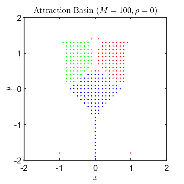
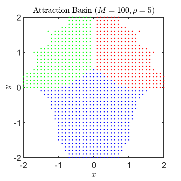
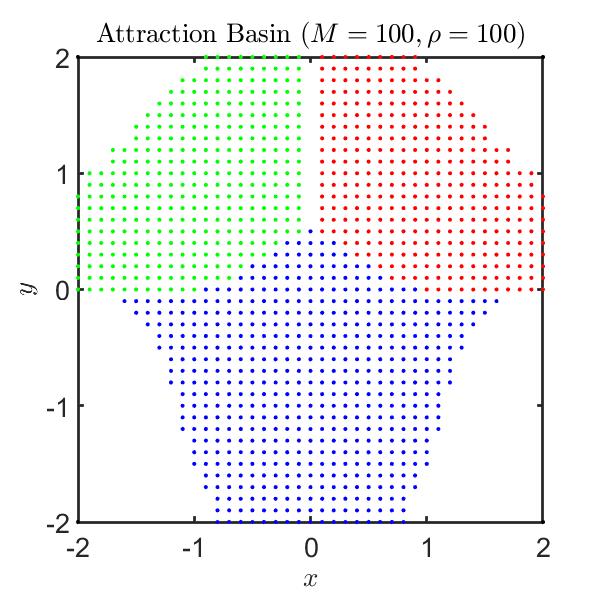
Figure 2: Comparison of attraction basins towards each of three saddle points when $\rho$ varies. The index-1 region $\Omega_{1}$ of the function $V$ is also shown.

We test different combinations of $\rho$ and $M$ on this example for the IPM algorithm. Figure 1 shows how the errors decay. For small $M$, the minimization subproblem in each iteration is solved very inexactly and the penalty function $d(x,y)$ can barely take effects. So, the difference in the value of $\rho$ leads to little difference in results. If $M$ is large, the effect of $\rho$ becomes very important to maintain the convergence. In the last panel of Figure 1, we deliberately select a bad initial point to show the interesting effect that the increasing penalty factor can improve the convergence by suppressing the oscillations.

We further test the convergence behaviours by examining the basin of attraction of our IPM scheme at $M=100$. Figure 2 exhibits the attraction basin, which is the collection of initial points that our scheme converges to one of three saddle points under different values of $\rho$. We can see that the attraction basin significantly expands at $\rho=5$. When $\rho=100$, the basin of attraction can cover the whole index-1 region $\omega_{1}$. $x\in\Omega_{1}$ is a sufficient condition for the minimization problem in each step of iteration to be globally convex as stated in Theorem 1, from which we inferred that $x_{0}\in\Omega_{1}$ is a sufficient condition for the iterative minimization proximal minimization scheme to converge to a saddle point. And this aligns with the observations in this numerical experiment.

5.2 Cahn-Hilliard equation

The second example is Cahn-Hilliard equation, which has been widely used in many complicated moving interface problems in material sciences and fluid dynamics through a phase-field approach [30, 7]. Consider the Ginzburg-Landau free energy on a one dimensional interval $[0,1]$

(21) $$F(\phi)=\int_{\Omega}\left[\frac{\kappa^{2}}{2}|\nabla\phi(x)|^{2}+f(\phi(x))\right]\,dx,\quad f(\phi)=(\phi^{2}-1)^{2}/4,$$

with $\kappa=0.04$ and the constant mass $\int\phi dx=0.6$. The Cahn-Hilliard (CH) equation [3] is the $H^{-1}$-gradient flow of $F(\phi)$,

(22) $$\frac{\partial\phi}{\partial t}=\Delta\frac{\delta F}{\delta\phi}=-\kappa^{2}\Delta^{2}\phi+\Delta(\phi^{3}-\phi).$$

Here $\frac{\delta F}{\delta\phi}$ is the first order variation of $F$ in the standard $L^{2}$ sense.

We are interested in the transition state of the Cahn-Hilliard equation, which is the index-1 saddle point of Ginzburg-Landau free energy in $H^{-1}$ Riemannian metric. However, in the calculation by the original IMF[11, 16], the convergence effect relies on a good initial state as well as the inner iteration number $M$. In the IPM method, we take $d(x,y)=|x-y|^{4}$, the auxiliary functional then becomes

(23) $$\widetilde{W}_{\rho}(\phi,\phi^{(k)})=\int_{\Omega}\Big{[}\frac{\kappa^{2}}{2}|\nabla\phi|^{2}+f(\phi)-\kappa^{2}|\nabla\hat{\phi}|^{2}-2f(\hat{\phi})\Big{]}\,dx+\rho\int_{\Omega}|\phi-\phi^{(k)}|^{4}\,dx.$$

The gradient flow of $\widetilde{W}_{\rho}(\phi,\phi^{(k)})$ in $H^{-1}$ metric is $\frac{\partial\phi}{\partial t}=\Delta\delta_{\phi}\widetilde{W}_{\rho}(\phi),$ with $\delta_{\phi}\widetilde{W}_{\rho}(\phi)=-\kappa^{2}\Delta\phi+(\phi^{3}-\phi)+2\left\langle\mathbf{v}_{1},\kappa^{2}\Delta\hat{\phi}-(\hat{\phi}^{3}+\hat{\phi})\right\rangle_{L^{2}}\mathbf{v}_{1}+4\rho(\phi-\phi^{(k)})^{3},$ and $\hat{\phi}=\phi^{(k)}+\left\langle\mathbf{v}_{1},\phi-\phi^{(k)}\right\rangle_{H^{-1}}\mathbf{v}_{1}$.

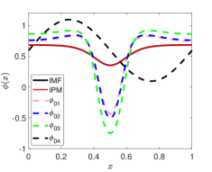
(a) Transition state

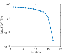
(b) Decay of error

Figure 3: (a): Transition state (solid curves) computed by the IMF and IPM from different initial states. The pink, blue and green dashed lines are the initial states correspond to the three states in Table 2 which are taken from the minimum energy path, while the dark dashed line is from the initial $\phi_{04}=\sin(2\pi x)$. (b): The decay of the error $\|\Delta\delta_{\phi}F(\phi^{(k)})\|_{L^{2}}$ measured by the $L^{2}$ norm of the $H^{-1}$-gradient.

In the numerical simulation, we take $\rho=100$ for the penalty factor and use the uniform mesh grid for spatial discretization $\{x_{i}=ih,i=0,1,2,\ldots,N\}.~{}h=1/N.$ $N=100$, $\Delta t=0.1$. The periodic boundary condition is considered. The saddle point of $F(\phi)$ is reproduced (see Figure 3a), which is the same as the result in the references[16, 14]. Besides, the quadratic convergence rate of the IPM algorithm is also verified empirically; see Figure 3b. In order to illustrate the advantage of this method, we make comparison of the convergence results between the original IMF ($\rho=0$) and the proximal method ($\rho=100$) here, starting from different initial states and with the different inner iteration number $M$. Table 2 shows the convergence/divergence results for three initial states $\phi_{01},\phi_{02}$ and $\phi_{03}$. The convergence/divergence result for the initial $\phi_{04}$ is the same as the result for $\phi_{03}$. We find that the farther the initial state is away from the saddle point, the smaller number of inner iterations the original IMF can tolerate, but the IPM can ensure convergence regardless of all initial states and inner iteration numbers tested here.

Table 2: Comparison of numerical convergence from three differential initial guesses $\phi_{01}$,$\phi_{02}$ and $\phi_{03}$ shown in Figure 3a. “IMF" means the original IMF; “ IPM" is the new method of iterative proximal minimization in this paper. $M$ is the number of gradient descent steps in minimizing the auxiliary functions. “$\checkmark$" and “✗" mean the convergent and divergent results, respectively.

$M$	$\phi_{01}$		$\phi_{02}$		$\phi_{03}$
	IMF	IPM	IMF	IPM	IMF	IPM
10	$\checkmark$	$\checkmark$	$\checkmark$	$\checkmark$	$\checkmark$	$\checkmark$
100	$\checkmark$	$\checkmark$	$\checkmark$	$\checkmark$	✗	$\checkmark$
200	$\checkmark$	$\checkmark$	✗	$\checkmark$	✗	$\checkmark$
500	✗	$\checkmark$	✗	$\checkmark$	✗	$\checkmark$

6 Conclusion

The calculation of relevant index-1 saddle points to transitions on a potential energy surface is an important computational task for rare event and phase transitions in chemistry and material science. We have established the equivalent connection between the index-1 saddle point of any function $V$ with continuous Hessian and the Nash equilibrium of a differential game constructed based on the iterative minimization formulation [11] for saddle points. The numerical contribution is a new iterative minimization algorithm with the proximal penalty function to enhance the robustness. The generalization to any Morse index $k$ is also discussed. The saddle-point calculation is in general still a formidable challenge compared to the gradient descent method for minimum points. It might be rewarding for a further exploration of the existing saddle-point search methods based on the minimal mode and the algorithmic game theory.

References

- [1] D. Balduzzi, S. Racaniere, J. Martens, J. Foerster, K. Tuyls, and T. Graepel, The mechanics of n-player differentiable games, in International Conference on Machine Learning, PMLR, 2018, pp. 354–363.
- [2] P. G. Bolhuis, D. Chandler, C. Dellago, and P. L. Geissler, Transition path sampling: Throwing ropes over rough mountain passes, in the dark, Annual Review of Physical Chemistry, 53 (2002), pp. 291–318. PMID: 11972010.
- [3] J. W. Cahn and J. E. Hilliard, Free energy of a nonuniform system. i. interfacial free energy, The Journal of Chemical Physics, 28 (1958), pp. 258–267.
- [4] C. J. Cerjan and W. H. Miller, On finding transition states, J. Chem. Phys., 75 (1981), pp. 2800–2806.
- [5] Y. Choi and P. McKenna, A mountain pass method for the numerical solution of semilinear elliptic problems, Nonlinear Analysis: Theory, Methods & Applications, 20 (1993), pp. 417–437.
- [6] G. M. Crippen and H. A. Scheraga, Minimization of polypeptide energy : XI. the method of gentlest ascent, Arch. Biochem. Biophys., 144 (1971), pp. 462–466.
- [7] H. Dang, P. C. Fife, and L. A. Peletier, Saddle solutions of the bistable diffusion equation, Ztschrift Für Angewandte Mathematik Und Physik Zamp, 43 (1992), pp. 984–998.
- [8] W. E, W. Ren, and E. Vanden-Eijnden, String method for the study of rare events, Phys. Rev. B, 66 (2002), p. 052301.
- [9] , Simplified and improved string method for computing the minimum energy paths in barrier-crossing events, J. Chem. Phys., 126 (2007), p. 164103.
- [10] W. E and X. Zhou, The gentlest ascent dynamics, Nonlinearity, 24 (2011), p. 1831.
- [11] W. Gao, J. Leng, and X. Zhou, An iterative minimization formulation for saddle point search, SIAM J. Numer. Anal., 53 (2015), pp. 1786–1805.
- [12] , Iterative minimization algorithm for efficient calculations of transition states, J. Comput. Phys., 309 (2016), pp. 69 – 87.
- [13] I. Gemp, B. McWilliams, C. Vernade, and T. Graepel, Eigengame: PCA as a Nash equilibrium, arXiv preprint arXiv:2010.00554, (2020).
- [14] S. Gu, L. Lin, and X. Zhou, Projection method for saddle points of energy functional in metric, Journal of scientific computing, 89 (2021), pp. 1–17.
- [15] S. Gu and X. Zhou, Multiscale gentlest ascent dynamics for saddle point in effectve dynamics of slow-fast system, Commun. Math. Sci., 15 (2017), pp. 2279–2302.
- [16] S. Gu and X. Zhou, Convex splitting method for the calculation of transition states of energy functional, J. Comput. Phys., 353 (2018), pp. 417–434.
- [17] S. Gu and X. Zhou, Simplified gentlest ascent dynamics for saddle points in non-gradient systems, Chaos: An Interdisciplinary Journal of Nonlinear Science, 28 (2018), p. 123106.
- [18] G. Henkelman and H. Jónsson, A dimer method for finding saddle points on high dimensional potential surfaces using only first derivatives, J. Chem. Phys., 111 (1999), pp. 7010–7022.
- [19] H. Jònsson, G. Mills, and K. W. Jacobsen, Nudged elasic band method for finding minimum energy paths of transitions, in Classical and Quantum Dynamics in Condensed Phase Simulations, B. J. Berne, G. Ciccotti, and D. F. Coker, eds., New Jersey, 1998, LERICI, Villa Marigola,Proceedings of the International School of Physics, World Scientific, p. 385.
- [20] J. Leng, W. Gao, C. Shang, and Z.-P. Liu, Efficient softest mode finding in transition states calculations, J. Chem. Phys., 138 (2013), p. 094110.
- [21] A. Letcher, D. Balduzzi, S. Racaniere, J. Martens, J. Foerster, K. Tuyls, and T. Graepel, Differentiable game mechanics, The Journal of Machine Learning Research, 20 (2019), pp. 3032–3071.
- [22] A. Levitt and C. Ortner, Convergence and cycling in walker-type saddle search algorithms, SIAM J. Numer. Anal., 55 (2017).
- [23] C. Li, J. Lu, and W. Yang, Gentlest ascent dynamics for calculating first excited state and exploring energy landscape of Kohn-Sham density functionals, The Journal of Chemical Physics, 143 (2015), p. 224110.
- [24] Y. Li and J. Zhou, A minimax method for finding multiple critical points and its applications to semilinear pdes, SIAM J Sci Comput, 23 (2001), pp. 840–865.
- [25] J. F. Nash Jr, Equilibrium points in n-person games, Proceedings of the national academy of sciences, 36 (1950), pp. 48–49.
- [26] S. Omidshafiei, K. Tuyls, W. M. Czarnecki, F. C. Santos, M. Rowland, J. Connor, D. Hennes, P. Muller, J. Pérolat, B. D. Vylder, et al., Navigating the landscape of multiplayer games, Nature communications, 11 (2020), pp. 1–17.
- [27] M. J. Osborne and A. Rubinstein, A course in game theory, MIT press, 1994.
- [28] W. Ren and E. Vanden-Eijnden, A climbing string method for saddle point search, J. Chem. Phys., 138 (2013), p. 134105.
- [29] A. Samanta and W. E, Atomistic simulations of rare events using gentlest ascent dynamics, J. Chem. Phys., 136 (2012), p. 124104.
- [30] J. Shen and X. Yang, Numerical approximations of allen-cahn and cahn-hilliard equations, Discrete and Continuous Dynamical Systems, 28 (2010), pp. 1669–1691.
- [31] D. J. Wales, Energy Landscapes with Application to Clusters, Biomolecules and Glasses, Cambridge University Press, 2003.
- [32] Z. Xie, Y. Yuan, and J. Zhou, On finding multiple solutions to a singularly perturbed Neumann problem, SIAM J Sci Comput, 34 (2012), p. A395.
- [33] J. Yin, L. Zhang, and P. Zhang, High-index optimization-based shrinking dimer method for finding high-index saddle points, SIAM Journal on Scientific Computing, 41 (2019), pp. A3576–A3595.
- [34] J. Zhang and Q. Du, Shrinking dimer dynamics and its applications to saddle point search, SIAM J. Numer. Anal., 50 (2012), pp. 1899–1921.
- [35] L. Zhang, Q. Du, and Z. Zheng, Optimization-based shrinking dimer method for finding transition states, SIAM J. Sci. Comput., 38 (2016), pp. A528–A544.
- [36] L. Zhang, W. Ren, A. Samanta, and Q. Du, Recent developments in computational modelling of nucleation in phase transformations, npj Computational Materials, 2 (2016), p. 16003.