Power Spectra of Slow-Roll inflation in the consistent $D\to 4$ Einstein-Gauss-Bonnet gravity

Abstract

The slow-roll inflation which took place at extremely high energy regimes is in general believed to be sensitive to the high-order curvature corrections to the classical general relativity (GR). In this paper, we study the effects of the high-order curvature term, the Gauss-Bonnet (GB) term, on the primordial scalar and tensor spectra of the slow-roll inflation in the consistent $D\to 4$ Einstein Gauss-Bonnet (4EGB) gravity. The GB term is incorporated into gravitational dynamics via the re-scaling of the GB coupling constant $\alpha\to\alpha/(D-4)$ in the limit $D\to 4$. For our purpose, we calculate explicitly the primordial scalar and tensor power spectra with GB corrections accurate to the next-to-leading order in the slow-roll approximation in the slow-roll inflation by using the third-order uniform asymptotic approximation method. The corresponding spectral indices and their runnings of the spectral indices for both the scalar and tensor perturbations as well as the ratio between the scalar and tensor spectra are also calculated up to the next-to-leading order in the slow-roll expansions. These results represent the most accurate results obtained so far in the literature. In addition, by studying the theoretical predictions of the scalar spectral index and the tensor-to-scalar ratio with Planck 2018 constraint in a model with power-law potential, we show that the second-order corrections are important in future measurements.

I Introduction

The inflationary theory provides a successful solution to the problems of the standard big bang cosmology for instance the flatness problem and the horizon problem. It also explains successfully the almost scale-invariant and nearly Gaussian spectra of primordial density perturbations Guth:1980zm ; Starobinsky:1980te ; Sato:1980yn ; Baumann:2009ds , which eventually evolute to generate the large-scale structure (LSS) observed today in the universe and the cosmic microwave background (CMB) temperature anisotropies, which have been detected with high precision by WMAP WMAP:2010qai ; Larson:2010gs , PLANCK Planck:2015sxf ; Planck:2015zfm , and other CMB experiments.

Inflation took place at an extremely high energy regime in the early universe. In this regime, the standard theory of the slow-roll inflation in GR also suffers from several conceptional problems, such as the trans-Planckian problem Martin:2000xs ; Brandenberger:2012aj and the initial singularity problem Borde:1993xh ; Borde:2001nh . This is because the classical GR is usually expected to be broken down at such an extremely high energy regime. Thus, the inflationary theory in GR with some corrections can be regarded as the effective theory of the complete UV quantum gravity. This has led to a large amount of research works for considering possible high-order curvature corrections to slow-roll inflation that arise from radiative corrections of quantum gravity, for example, Horava-Lifshitz gravity Wang:2017brl and string/M-theory Baumann:2014nda .

The most important high-order curvature terms are the GB term and its Lovelock generalization, which have been extensively studied in various alternative theories beyond GR. However, because the GB term is a topological invariant in four dimensions, this term can have contributions to the gravitational dynamics only when it is coupled to a matter field. Latterly, Glavan and Lin formulated a new theory with GB term in four dimensions (4EGB) by rescaling the GB coupling constant $\alpha\rightarrow\alpha/(D-4)$ in the limit $D\rightarrow 4$ Glavan:2019inb . With this scaling, it is argued that in the limit $D\rightarrow 4$, the GB term can make nontrivial contributions to the gravitational dynamics. The 4EGB gravity has been extended to higher-order Lovelock gravity in Hennigar:2020lsl ; Fernandes:2020nbq . However, there are also certain criticisms of the new 4EGB theory Ai:2020peo ; Gurses:2020ofy ; Lu:2020iav ; Kobayashi:2020wqy ; Hennigar:2020lsl ; Fernandes:2020nbq ; Shu:2020cjw ; Bonifacio:2020vbk ; Mahapatra:2020rds . Someone argued that this theory lacks an intrinsically four-dimensional description in terms of a covariantly-conserved rank-2 tensor in four dimensions Gurses:2020ofy . The vacua of the model are ill-defined too Shu:2020cjw . Several variants of the 4EGB theory are proposed for the purpose of curing these problems, It is shown that by compressing a higher dimensional theory down to a $D-4$ dimensional maximally symmetric space and redefining a few parameters, the 4EGB theory can be reformulated to a specific class of the Horndeski theory Lu:2020iav . Its reformulation and Lovelock generalization as a scalar-tensor theory have been deduced Kobayashi:2020wqy ; Lu:2020iav . In these realizations, the original 4EGB theory is reformulated to a scalar-tensor theory, with a coupling between the scalar field and the GB term. And thus such theories, in general, propagate three degrees of freedom. Note that in such a scalar-tensor extension, it is also shown that the scalar field could be strongly coupled in a cosmological background Kobayashi:2020wqy and in a flat background Bonifacio:2020vbk . Another way to cure the pathologies of the original 4EGB theory is to break time diffeomorphism invariance but preserve the spatial one Aoki:2020lig . It is shown that this spatial covariant 4EGB gravity (i.e. the consistent $D\to 4$ Einstein-Gauss-Bonnet gravity) can only have two degrees of freedom due to a Lagrangian multiplier term in the gravitational action Aoki:2020lig .

In this paper, we will especially pay attention to the spatial covariant 4EGB gravity in the early universe, and their corrections to the standard slow-roll inflationary perturbations. It is interesting to note that the GB corrections to slow-roll inflationary spectra in the scalar-Gauss-Bonnet gravity have already been investigated and expanded at length in several works Jiang:2013gza ; Guo:2010jr ; Koh:2014bka ; Satoh:2010ep ; Satoh:2008ck ; vandeBruck:2015gjd ; Satoh:2007gn ; Chakraborty:2018scm . These papers have studied the primordial perturbation spectra with the GB corrections, and compared it with observed values. It is interesting to note that in the slow-roll inflation, the coupling between the scalar field and the GB term generates a time-dependent sound speed related to the equation of motion for scalar and tensor perturbations. In the spatial covariant 4EGB theory, it not only predicts time-dependent sound speeds associated with the tensor perturbations in the slow-roll inflation but also modifies the linear dispersion relation of the tensor modes. The primordial power spectra and non-Gaussianities with both the effects of the time-dependent sound speeds and modified dispersion have been explored in Aoki:2020ila . However, for calculating the perturbation spectra, the previous works have supposed this time-dependent sound speed as well as the slow-roll quantities as constants. In fact, this approach will be invalid when it is used to calculate the primordial spectra above the first-order in the slow-roll approximation.

With the emergence of new high-accuracy cosmological data, such as the Planck data, one expects to get tighter constraints on the theory. Thus, it is important to compare the theoretical predictions of specific inflation models with the observational data. With the rapid development of technology, the CMB observations and the incoming large-scale structures surveys will become more and more accurate. For example, the data from the stage-4 CMB experiments and the LiteBird satellite provide will not only increase the sensitivity of primordial gravitational waves ($\epsilon_{1}$) but also explore much higher multipoles CMB-S4:2016ple ; SimonsObservatory:2018koc ; Mallaby-Kay:2021tuk ; LiteBIRD:2022cnt ; Auclair:2022yxs . The Euclid satellite and other ground surveys are going to measure the small scales in the matter power spectrum LSSTScience:2009jmu ; Lacasa:2019flz ; Euclid:2021qvm ; Auclair:2022yxs . All these measurements will be sensitive to the high-order corrections to the slow-roll perturbation spectra beyond the leading-order in the slow-roll approximations Adshead:2010mc ; Martin:2014rqa ; Sprenger:2018tdb . In this situation, in order to analyze the data with future observations, the theoretical predictions must be more precise and go beyond the leading slow-roll orders Auclair:2022yxs ; Martin1 ; Martin2 .

With these considerations, it is highly demanded to consider the slow-roll approximation beyond the leading-order in the calculations of the inflationary perturbation spectra. For this purpose, one has to consider both the effects of the time variation of the sound speeds and the modified dispersion relation that arise in the spatial covariant 4EGB theory. Both the time-dependent propagating sound speeds and the modified dispersion relation can make important corrections in the primordial scalar and tensor perturbation spectra. However, considerations of the time variation of the sound speed and the modified dispersion relation make it very difficult to calculate the corresponding power spectra. In this paper, in order to calculate the primordial perturbation spectra and their spectral indices to desired precision, we employ the uniform asymptotic approximation developed in a series of papers Zhu:2013fha ; Zhu:2013upa ; Zhu:2014wfa ; Zhu:2015ata ; Zhu:2016srz ; Zhu:2014wda ; Zhu:2014aea ; Zhu:2015xsa ; Zhu:2015owa . This approximation provides a better treatment to equations with turning points and poles, and has been widely applied in calculating primordial spectra for various inflation models Zhu:2013fha ; Zhu:2013upa ; Zhu:2014wfa ; Zhu:2015ata ; Zhu:2016srz ; Zhu:2014wda ; Zhu:2014aea ; Zhu:2015xsa ; Zhu:2015owa and applications in studying the reheating process Zhu:2018smk and quantum mechanics Li:2019cre . The main goal of this paper is to use the uniform asymptotic approximation to calculate the inflationary observables of the slow-roll inflation in the spatial covariant 4EGB theory with high accuracy.

The content of the paper is arranged as follows. In Sec. II, we present a brief introduction of spatial covariant 4EGB gravity, and in Sec. III, we consider the cosmological perturbations in a flat FRW background, including the linear scalar perturbations and tensor perturbations. Then we calculate explicitly the power spectra, spectral indices, and runnings of the spectral indices of both scalar and tensor perturbations and the ratio between the scalar and tensor spectra in the slow-roll inflation with the GB correction in Sec. IV. With the obtained expressions of the scalar spectral index and the tensor-to-scalar ratio, we study their predictions with Planck 2018 constraint in a model for specific power-law potential in Sec. V. Our main conclusions and outlook are summarized in Sec. VI. We also give the most general formulas for calculating the primordial power spectra in the high-order uniform asymptotic approximations in appendixes A and B.

II spatial covariant 4EGB gravity

In this section, we will briefly introduce the spatial covariant 4EGB gravity. The details of this theory can be found in Glavan:2019inb ; Aoki:2020lig . In this theory, the dynamical variables are the shift vector $N^{i}$, lapse function $N$ and spatial metric $\gamma_{ij}$. We can write the metric of a spacetime in the Arnowitt-Deser-Misner (ADM) form,

$$ds^{2}=-N^{2}dt^{2}+\gamma_{ij}(dx^{i}+N^{i}dt)(dx^{j}+N^{j}dt).$$ (2.1)

The action of this theory is as follows,

$$S_{\rm EGB}^{\rm 4D} = \int dtd^{3}x\sqrt{\gamma}N{\cal{L}}^{\rm 4D}_{\rm EGB}$$ (2.2)

here $\gamma$ is the determinate of the spatial metric $\gamma_{ij}$ with $\gamma={\rm det}(\gamma_{ij})$ , and

$${\cal{L}}^{\rm 4D}_{\rm EGB} = \frac{M_{\rm Pl}^{2}}{2}\Bigg{[}2R-{\cal M}+\frac{\tilde{\alpha}}{2}\Big{(}8R^{2}-4R{\cal M}-{\cal M}^{2}$$

$$-\frac{8}{3}\left(8R_{ij}R^{ij}-4R_{ij}{\cal M}^{ij}-{\cal M}_{ij}{\cal M}^{ij}\right)\Big{)}\Bigg{]},$$

with

$${\cal M}_{ij} \equiv R_{ij}+{\cal K}^{k}_{k}{\cal K}_{ij}-{\cal K}_{ik}{\cal K}^{k}_{j},$$ (2.4)

$${\cal M} \equiv {\cal M}^{i}_{i},$$ (2.5)

$${\cal K}_{ij} \equiv \frac{1}{2N}\left(\partial_{t}\gamma_{ij}-2D_{(i}N_{j)}-\gamma_{ij}D^{2}\lambda_{\rm GF}\right).$$ (2.6)

In the above, $M_{\rm Pl}^{2}=1/(8\pi G)$ is the reduced Planck mass, where $G$ being the Newton gravitational coupling constant. $R$, $R_{ij}$ here are respectively the Ricci scalar and the Ricci tensor refer to the spatial-metric $\gamma_{ij}$. $D_{i}$ is the covariant derivative and can be compatible with the spatial metric. $\lambda_{\rm GF}$ is similar to the Lagrange multipliers, and it imposes a primary constraint on the theory such that it can propagate only two degrees of freedom Glavan:2019inb ; Aoki:2020lig . The coupling constant $\tilde{\alpha}$ is the rescaled GB coupling constant $\tilde{\alpha}\to\alpha/(D-4)$ with the limit $D\to 4$.

One important feature of the spatial covariant 4EGB gravity is that it don’t admit the full diffeomorphism invariance of the four-dimensional spacetime, but break the temporal diffeomorphism. Then this theory only has the time reparametrization symmetry and the three-dimensional spatial diffeomorphism,

$$t \to \tilde{t}=t-f(t),$$ (2.7)

$$x^{i} \to \tilde{x}^{i}=x^{i}-\zeta^{i}(t,x^{j}).$$ (2.8)

where $f(t)$ and $\zeta^{i}(t,x^{j})$ are the the infinitesimal generators of the time reparametrization and the spatial diffeomorphism, respectively. With this gauge transformation, the dynamical variables $N$, $N_{i}$, and $\gamma_{ij}$ can transform as

$$\delta N = \zeta^{k}D_{k}N+\dot{N}f+N\dot{f},$$

$$\delta N_{i} = N_{k}D_{i}\zeta^{k}+\zeta^{k}D_{k}N_{i}+\gamma_{ik}\dot{\zeta}^{k}+\dot{N}_{i}f+N_{i}\dot{f},$$

$$\delta\gamma_{ij} = D_{i}\zeta_{j}+D_{j}\zeta_{i}+f\dot{\gamma}_{ij}.$$ (2.9)

Here a dot is the derivative of respect to the time $t$.

III Cosmological perturbations in a flat FRW background

In this section, we present a brief introduction of the scalar and tensor perturbations of the slow-roll inflation in the spatial covariant 4EGB gravity.

III.1 Slow-roll inflation

For later convenience to introduce the cosmological perturbations, we first consider a flat Friedmann-Robertson-Walker (FRW) background,

$$ds^{2} = -dt^{2}+a^{2}(t)\delta_{ij}dx^{i}dx^{j}$$ (3.1)

$$= a^{2}(\tau)(-d\tau^{2}+\delta_{ij}dx^{i}dx^{j}),$$

where $a(t)$ is the scalar factor of the universe , $t$ is the cosmic time, and $\tau$ is the conformal time. For studying the inflationary cosmology and cosmological perturbations, we can consider the theory in (2.2) with a scalar field $\phi$ with a potential $V(\phi)$, that is

$$S=S_{\rm EGB}^{\rm 4D}+S_{\phi}$$ (3.2)

where

$$S_{\phi}=\int dtd^{3}x\sqrt{\gamma}N\left[\frac{1}{2}g^{\mu\nu}\partial_{\mu}\phi\partial_{\nu}\phi+V(\phi)\right].$$ (3.3)

Here the scalar field $\phi$ is canonical and coupled to gravity minimally, $\phi$ is the inflation field with potential $V(\phi)$, and $g^{\mu\nu}$ is the metric of the 4-dimensional spacetime. Thus the modified Friedmann and the Klein-Gordon equations in the spatial covariant 4EGB gravity can be written as Glavan:2019inb ; Aoki:2020lig

$$3M_{\rm Pl}^{2}(H^{2}+\tilde{\alpha}H^{4})=\frac{1}{2}\dot{\phi}^{2}+V(\phi),$$ (3.4)

$$-2M_{\rm Pl}^{2}(1+2\tilde{\alpha}H^{2})\dot{H}=\dot{\phi}^{2},$$ (3.5)

and

$$\ddot{\phi}+3H\dot{\phi}+V_{,\phi}=0,$$ (3.6)

where $H\equiv\dot{a}/a$ is the Hubble parameter with a dot is the derivative with respect to the cosmic time $t$, and $V_{,\phi}=dV(\phi)/d\phi$. With these equations of the background evolutions, we will respectively consider the cosmological scalar and tensor perturbations in the following subsections.

To consider the slow-roll inflation, we also need to impose the following slow-roll conditions

$$\frac{1}{2}\dot{\phi}^{2}\ll V,\;\;|\ddot{\phi}|\ll|3H\dot{\phi}|.$$ (3.7)

Then we can easily introduce the Hubble flow slow-roll parameters $\epsilon_{n}$. The definitions of the Hubble flow slow-roll parameters are

$$\epsilon_{n+1}\equiv\frac{d\ln\epsilon_{n}}{d\ln a},\;\;\epsilon_{1}\equiv-\frac{\dot{H}}{H^{2}}.$$ (3.8)

The conformal time $\tau$ is defined as

$$\tau(t)=\int^{t}_{t_{\text{end}}}\frac{dt^{\prime}}{a(t^{\prime})},$$ (3.9)

where $t_{\text{end}}$ is the time of the slow-roll inflation ends. We also introduce a new parameter to represent the GB effects and simplify the calculation, which is defined as

$$f_{\rm GB}=2\tilde{\alpha}H^{2}.$$ (3.10)

During the slow-roll inflation, this parameter is also slow-varying , and it characterizes the correction of the GB term in the spatial covariant 4EGB gravity. In the slow-roll approximation, we treat this parameter as a new slow-roll parameter in the slow-roll expansion. In principle, the value of the paramater $f_{\rm GB}$ is not necessary to be at the order to of $\mathcal{O}(\epsilon)$. However, in orde to simplfy the calcualtions of the power spectra later, we assume that $f_{\rm\rm GB}\sim\mathcal{O}(\epsilon)$. Thus the calculations presented in this paper are valid only with this condition.

III.2 Scalar perturbations

Let us consider the linear scalar perturbations around the flat FRLW spacetime in the spatial covariant 4EGB gravity. It is more convenient to use the conformal time $\tau$ to achieve this purpose, and the background variables $(N,N^{i},\gamma_{ij})$ is as follows

$$\hat{N}=a(\tau),\;\;\hat{N}^{i}=0,\;\;\hat{\gamma}_{ij}=a^{2}(\tau)\delta_{ij},$$ (3.11)

where the quantities with a hat denote the background fields only depend on $\tau$. Under this background, we can introduce the scalar perturbations $(A,B,\psi,E,\delta\phi,\delta\lambda)$ as,

$$N=a(\tau)(1+A),\;\;N^{i}=\delta^{ij}\partial_{j}B,$$

$$\gamma_{ij}=a^{2}(\tau)[(1+2\psi)\delta_{ij}+2\partial_{i}\partial_{j}E],$$

$$\phi=\hat{\phi}+\delta\phi,\;\;\;\lambda_{\rm GF}=\hat{\lambda}_{\rm GF}+a^{2}\delta\lambda.$$ (3.12)

Here $\hat{\phi}$ and $\hat{\lambda}_{\rm GF}$ are the background fields of $\phi$ and $\lambda_{\rm GF}$ respectively, and only depends on $\tau$. With the gauge transformation (2.9), the scalar perturbations can transform in the form

$$A\to\tilde{A} = A+f^{\prime}+\mathcal{H}f,$$ (3.13)

$$B\to\tilde{B} = B+\zeta^{\prime},$$ (3.14)

$$\psi\to\tilde{\psi} = \psi+\mathcal{H}f,$$ (3.15)

$$E\to\tilde{E} = E+\zeta.$$ (3.16)

Here we split $\zeta^{i}=\zeta^{,i}+\zeta_{\perp}^{i}$ with $\zeta_{\perp}^{i}$ being the transverse part of the vector $\zeta^{i}$. Because the sptaial covariant 4EGB gravity breaks the time diffeomorphism, one can chose a gauge like neither $A=0$ nor $\psi=0$. From gauge transformation has been discussed above, there are only two gauges can be chosen:

$$(i)\;\;B=0,\;\;{\rm or}\;\;(ii)\;\;E=0.$$ (3.17)

Thus, of the four scalar type metric perturbations $(A,B,\psi,E)$, only one of $(E,B)$ can be eliminated by choosing $\zeta(t,x^{i})$ in the gauge transformation. This is different from the theory of full diffeomorphism in 4-dimensional spacetime, where either $A$ or $\psi$ can also be eliminated by choosing $f$ freely.

Then we consider the comoving curvature perturbation $\cal{R}$, which is defined as

$${\cal{R}}=-\psi+\frac{\cal{H}}{\hat{\phi^{\prime}}}\delta\phi.$$ (3.18)

Under the above gauge transformation, it is not difficult to verify that $\mathcal{R}$ is still gauge-invariant even in the current setup. With this definition and a series of tedious calculations, we can obtain the second order action of the terms of $\mathcal{R}$ Glavan:2019inb ; Aoki:2020lig ,

$$S^{(2)}=M_{\rm Pl}^{2}\int d\tau d^{2}xa^{2}\epsilon_{1}(1+f_{\rm GB})\Big{[}{\cal R}^{\prime 2}+\partial^{2}{\cal R}^{2}\Big{]}.$$

With variation of this double-dip action with respect to ${\cal R}$, the equation of motion for the comoving curvature perturbation ${\cal R}$ is obtained as follows,

$$\mathcal{R}^{\prime\prime}+\left(2\mathcal{H}+\frac{\epsilon_{1}^{\prime}}{\epsilon_{1}}+\frac{f_{\rm GB}^{\prime}}{1+f_{\rm GB}}\right)\mathcal{R}^{\prime}-\partial^{2}\mathcal{R}=0.$$ (3.20)

We can define the mode function $u_{\mathcal{R}}$ in terms of the Fourier modes of curvature perturbations as $u_{\mathcal{R}}=z_{\mathcal{R}}\mathcal{R}_{k}$. Then the equation of motion (3.20) can be transformed into the form

$$u^{\prime\prime}_{\mathcal{R}}(\tau)+\left(k^{2}-\frac{z^{\prime\prime}_{\mathcal{R}}}{z_{\mathcal{R}}}\right)u_{\mathcal{R}}(\tau)=0.$$ (3.21)

Here a prime is the derivative with respect to the conformal time $\tau$. $z_{\mathcal{R}}$ and $\frac{z^{\prime\prime}_{\mathcal{R}}}{z_{\mathcal{R}}}$ can be written as follows

$$z_{\mathcal{R}} = a\sqrt{2\epsilon_{1}(1+f_{\rm GB})}M_{\rm Pl},$$ (3.22)

and

$$\frac{z^{\prime\prime}_{\mathcal{R}}}{z_{\mathcal{R}}} = 2a^{2}H^{2}\Bigg{[}1-\frac{1+4f_{\rm GB}}{2(1+f_{\rm GB})}\epsilon_{1}+\frac{3}{4}\epsilon_{2}$$ (3.23)

$$~{}~{}~{}~{}~{}~{}~{}~{}+\frac{(3+2f_{\rm GB})f_{\rm GB}}{2(1+f_{\rm GB})^{2}}\epsilon_{1}^{2}-\frac{1+5f_{\rm GB}}{4(1+f_{\rm GB})}\epsilon_{1}\epsilon_{2}$$

$$~{}~{}~{}~{}~{}~{}~{}~{}+\frac{\epsilon_{2}^{2}}{8}+\frac{1}{4}\epsilon_{2}\epsilon_{3}\Bigg{]}.$$

III.3 Tensor perturbations

The cosmological tensor perturbations $h_{ij}$ is defined as,

$$\delta\gamma_{ij}=a^{2}h_{ij},\;\delta N^{i}=0,\;\;\delta N=0,$$ (3.24)

where $h_{ij}$ denotes the traceless and transverse metric perturbations, namely,

$$\partial^{i}h_{ij}=0=h_{i}^{i}.$$ (3.25)

With the gauge transformation (2.9), the tensor perturbations are found to be gauge invariant. The above definition requires us to derive equations of motion for tensor perturbations. To this end, the metric perturbation can be first substituted into Eq. (3.2) and then expanded to the quadratic order of $h_{ij}$. After a series of complicated calculations, one obtains Glavan:2019inb ; Aoki:2020lig ,

$$S^{(2)}_{h} = \frac{M_{\rm Pl}^{2}}{8}\int d\tau d^{3}xa^{2}(\tau)\Big{[}(1+2\tilde{\alpha}H^{2})h^{\prime}_{ij}h^{\prime ij}$$ (3.26)

$$\;\;\;\;-\left(1+2\tilde{\alpha}H^{2}+4\tilde{\alpha}\dot{H}\right)\partial_{k}h_{ij}\partial^{k}h^{ij}$$

$$~{}~{}~{}~{}-\frac{4\tilde{\alpha}}{a^{2}(\tau)}\partial^{2}h_{ij}\partial^{2}h^{ij}\Big{]}.$$

Then one can take the variation of the quadratic action of$h_{ij}$ to obtain the equations of motion of the tensor perturbations, which gives,

$$h_{ij}^{\prime\prime}+2\mathcal{H}\left(1+\frac{2\alpha\dot{H}}{1+2\alpha H^{2}}\right)h_{ij}^{\prime}$$

$$-\left(1+\frac{4\alpha\dot{H}}{1+2\alpha H^{2}}\right)\partial^{2}h_{ij}+\frac{4\alpha/a^{2}}{1+2\alpha H^{2}}\partial^{4}h_{ij}=0,$$

where $\mathcal{H}\equiv a^{\prime}/a$ with a prime representing the derivative with respect to the conformal time $\tau$.

In order to study the evolution of $h_{ij}$, we expand it to the spatial Fourier harmonics,

$$h_{ij}(\tau,x^{i})=\sum_{A={\rm R,L}}\int\frac{d^{3}k}{(2\pi)^{3}}h_{A}(\tau,k^{i})e^{ik_{i}x^{i}}e_{ij}^{A}(k^{i}),$$

where $e_{ij}^{A}$ represent the circular polarization tensors. $e_{ij}^{A}$ satisfy the following relation

$$\epsilon^{ijk}n_{i}e_{kl}^{A}=i\rho_{A}e^{jA}_{~{}l},$$ (3.29)

where $\rho_{\rm L}=-1$ and $\rho_{\rm R}=1$. It is worth noting that the propagation equations of these two modes are decoupled, and can be transformed into

$$h_{A}^{\prime\prime}+\left(2\mathcal{H}+\frac{f_{\rm GB}^{\prime}}{1+f_{\rm GB}}\right)h_{A}^{\prime}+\omega_{k}^{2}h_{A}=0.$$ (3.30)

The quantity $\frac{f_{\rm GB}^{\prime}}{1+f_{\rm GB}}$ in parentheses gives a description of the correction of the friction term, while $\omega_{k}^{2}$ describes the correction of the dispersion relation for the tensor perturbations, which reads

$$\omega_{k}^{2} \equiv \left(1-\frac{8\alpha\dot{H}}{M_{\rm Pl}^{2}+4\alpha H^{2}}+\frac{4\tilde{\alpha}/a^{2}}{1+2\tilde{\alpha}H^{2}}k^{2}\right)k^{2}$$ (3.31)

$$= \left(1+\frac{2f_{\rm GB}\epsilon_{1}}{1+f_{\rm GB}}+\frac{2f_{\rm GB}}{1+f_{\rm GB}}\frac{k^{2}}{a^{2}H^{2}}\right)k^{2}$$

$$= c_{h}^{2}k^{2}+\frac{2f_{\rm GB}}{1+f_{\rm GB}}\frac{k^{2}}{a^{2}H^{2}}k^{2},$$

with

$$c_{h}^{2}\equiv 1+\frac{2f_{\rm GB}\epsilon_{1}}{1+f_{\rm GB}}.$$ (3.32)

We then define a new variable ${u_{h}=\frac{1}{2}z_{h}h_{A}}$ and change Eq. (3.30) to

$$u_{h}^{\prime\prime}+\left[\omega_{k}^{2}-\frac{z_{h}^{\prime\prime}}{z_{h}}\right]u_{h}=0,$$ (3.33)

where

$${z_{h}\equiv a\sqrt{1+f_{\rm GB}}M_{\rm{pl}}},$$ (3.34)

and

$$\frac{z_{h}^{\prime\prime}}{z_{h}} = 2a^{2}H^{2}\Bigg{[}1-\frac{1+4f_{\rm GB}}{2(1+f_{\rm GB})}\epsilon_{1}+\frac{(3+2f_{\rm GB})f_{\rm GB}}{2(1+f_{\rm GB})^{2}}\epsilon_{1}^{2}$$ (3.35)

$$~{}~{}~{}~{}~{}~{}~{}~{}~{}~{}~{}~{}~{}~{}~{}~{}~{}-\frac{f_{\rm GB}}{2(1+f_{\rm GB})}\epsilon_{1}\epsilon_{2}\Bigg{]}.$$

IV Scalar and Tensor Perturbation Spectra in the uniform asymptotic approximation

In this section, we calculated the scalar and tensor spectra of the slow-roll inflation in the spatial covariant 4EGB gravity. The power spectrum calculation method used in this paper is the uniform asymptotic approximation, and the third-order approximation of it are developed in a series papers Zhu:2013fha ; Zhu:2013upa ; Zhu:2016srz ; Zhu:2014wfa ; Zhu:2014wda ; Zhu:2014aea ; Zhu:2015xsa ; Zhu:2015owa ; Zhu:2015ata ; Zhu:2018smk . The general formulas for calculating the primordial power spectra from the slow-roll inflation are described in appendix A and B. The primordial power spectra for both the scalar and tensor perturbations are calculated up to the second-order in the slow-roll approximation in the following subsections.

IV.1 Scalar Spectrum

We first consider the scalar perturbations. In order to employ the uniform asymptotic approximation, we need to map the equation of motion of $u_{\cal R}$ in (3.21) into the standard form in (A.1). We have

$$\lambda^{2}\hat{g}(y)+q(y)=\frac{\nu_{\cal R}^{2}}{y^{2}}-1,$$ (4.1)

with

$$\lambda^{2}\hat{g}(y)=\tau^{2}\frac{z^{\prime\prime}_{\cal R}}{z_{\cal R}}\frac{1}{y^{2}},$$ (4.2)

$$q(y)=-\frac{1}{4y^{2}},$$ (4.3)

where

$$\nu_{\cal R}^{2} = \frac{1}{4}+\tau^{2}\frac{z^{\prime\prime}_{\cal R}}{z_{\cal R}}$$ (4.5)

$$= \frac{1}{4}+2\tau^{2}a^{2}H^{2}\Bigg{[}1-\frac{1+4f_{\rm GB}}{2(1+f_{\rm GB})}\epsilon_{1}+\frac{3}{4}\epsilon_{2}$$

$$+\frac{(3+2f_{\rm GB})f_{\rm GB}}{2(1+f_{\rm GB})^{2}}\epsilon_{1}^{2}-\frac{1+5f_{\rm GB}}{4(1+f_{\rm GB})}\epsilon_{1}\epsilon_{2}$$

$$+\frac{\epsilon_{2}^{2}}{8}+\frac{1}{4}\epsilon_{2}\epsilon_{3}\Bigg{]}$$

It is easy to see that the function $\lambda^{2}\hat{g}(y)$ has a single turning point $y_{0}(\bar{\tau}_{0})=-k\bar{\tau}_{0}$, which related to $\nu_{\cal R}$ as

$$y_{0}(\bar{\tau}_{0})=-k\bar{\tau}_{0}=\nu_{\cal R}(\bar{\tau}_{0}).$$ (4.6)

Hereafter we use a bar over the quantities denoting the quantities evaulated at the turning point.

In order to match the accuracy of forthcoming observations, we need to calculate the scalar spectrum and the corresponding spectral indices up to the next-to-leading order (second-order) in the expansions of the slow-roll approximation. For this purpose, we have to consider the time variations of the slow-roll quantities such as $\nu_{\cal R}$. Considering $\nu_{\cal R}$ is slowly varying, it is convenient to expand it up to the second-order in the slow-roll expansions as that presented in Eq. (B.2) in appendix B. For $\nu_{\mathcal{R}}$, the expansion coefficients $\bar{\nu}_{\mathcal{R}0}$, $\bar{\nu}_{\mathcal{R}1}$, and $\bar{\nu}_{\mathcal{R}2}$ in (B.2) can be calculated from Eqs.(4.5) and (3.22), we find

$$\bar{\nu}_{\mathcal{R}0} \simeq \frac{3}{2}+\bar{\epsilon}_{1}+\frac{\bar{\epsilon}_{2}}{2}-\bar{f}_{\text{GB}}\bar{\epsilon}_{1}+\bar{\epsilon}_{1}^{2}+\frac{11\bar{\epsilon}_{1}\bar{\epsilon}_{2}}{6}+\frac{\bar{\epsilon}_{2}\bar{\epsilon}_{3}}{6},$$

$$\bar{\nu}_{\mathcal{R}1} \simeq -\bar{\epsilon}_{1}\bar{\epsilon}_{2}-\frac{\bar{\epsilon}_{2}\bar{\epsilon}_{3}}{2},$$ (4.8)

and

$$\bar{\nu}_{\mathcal{R}2}\equiv\frac{d^{2}\nu_{\mathcal{R}}}{d\ln^{2}(-\tau)} = \mathcal{O}(\bar{\epsilon}_{i}^{3}).$$ (4.9)

Here a letter with an over bar means that the quantity is at the turning point $\bar{y}_{0}$.

Then, using the above expansions, the power spectrum for the curvature perturbation $\mathcal{R}$ can be calculated via Eq.(Appendix A: General formulas of primordial spectra in the uniform asymptotic approximation). After tedious calculations we obtain,

$$\Delta_{\mathcal{R}}^{2}(k) = \frac{181\bar{H}^{2}}{72e^{3}M_{\rm{pl}}^{2}\pi^{2}\bar{\epsilon}_{1}}\Big{[}1-\bar{f}_{\text{GB}}+\bar{f}_{\text{GB}}^{2}+\Big{(}2\ln{2}-\frac{496}{181}+\frac{630\bar{f}_{\text{GB}}}{181}-4\bar{f}_{\text{GB}}\ln{2}\Big{)}\bar{\epsilon}_{1}+\Big{(}\frac{67}{181}-\ln 2\Big{)}\Big{(}\bar{f}_{\text{GB}}-1\Big{)}\bar{\epsilon}_{2}$$ (4.10)

$$+ \Big{(}\frac{293}{181}-\frac{630\ln{2}}{181}+2\ln{2}\Big{)}\bar{\epsilon}_{1}^{2}-\Big{(}\frac{11}{362}+\frac{67\ln 2}{181}-\frac{\ln^{2}2}{2}\Big{)}\bar{\epsilon}_{2}^{2}$$

$$+ \Big{(}\frac{\pi^{2}}{12}-\frac{4231}{1629}+\frac{47\ln{2}}{181}+\ln^{2}2\Big{)}\bar{\epsilon}_{1}\bar{\epsilon}_{2}+\Big{(}\frac{\pi^{2}}{24}-\frac{86}{1629}+\frac{67\ln 2}{181}-\frac{\ln^{2}2}{2}\Big{)}\bar{\epsilon}_{2}\bar{\epsilon}_{3}\Big{]},$$

where $e$ is the natiral constant. From the scalar spectrum (4.10), we find that the parameter $\bar{f}_{\rm GB}$ enters into the scalar spectrum at the leading-order in the slow-roll expansion.

Then with the scalar power spectrum given above, the scalar spectral index is,

$$n_{\mathcal{R}}-1 \simeq -2\Big{(}1-\bar{f}_{\text{GB}}\Big{)}\bar{\epsilon}_{1}-\bar{\epsilon}_{2}-2\bar{\epsilon}_{1}^{2}$$

$$-\Big{(}\frac{677}{181}-2\ln{2}\Big{)}\bar{\epsilon}_{1}\bar{\epsilon}_{2}-\Big{(}\frac{67}{181}-\ln{2}\Big{)}\bar{\epsilon}_{2}\bar{\epsilon}_{3},$$

and the running of the scalar spectral index is expressed as

$$\alpha_{\mathcal{R}} \simeq -2\bar{\epsilon}_{1}\bar{\epsilon}_{2}-\bar{\epsilon}_{2}\bar{\epsilon}_{3}-4\bar{f}_{\text{GB}}\bar{\epsilon}_{1}^{2}+2\bar{f}_{\text{GB}}\bar{\epsilon}_{1}\bar{\epsilon}_{2}-6\bar{\epsilon}_{1}^{2}\bar{\epsilon}_{2}$$ (4.12)

$$-\Big{(}\frac{677}{181}-2\ln 2\Big{)}\bar{\epsilon}_{1}\bar{\epsilon}_{2}^{2}-\Big{(}\frac{858}{181}-2\ln 2\Big{)}\bar{\epsilon}_{1}\bar{\epsilon}_{2}\bar{\epsilon}_{3}$$

$$-\Big{(}\frac{67}{181}-\ln 2\Big{)}\Big{(}\bar{\epsilon}_{2}\bar{\epsilon}_{3}^{2}+\bar{\epsilon}_{2}\bar{\epsilon}_{3}\bar{\epsilon}_{4}\Big{)}.$$

For scalar spectral index, the new effects denoted by the slow-roll parameter $\bar{f}_{\rm GB}$ appears at the next-to-leading order, while for the running of the index, they only contribute to the third-order of the slow-roll approximation.

IV.2 Tensor Spectrum

Now we consider the tensor spectrum. First we need to derive the expressions of $\bar{\nu}_{h0},\bar{\nu}_{h1},\bar{b}_{h0},\bar{b}_{h1}$, and $\bar{c}_{h0}$, which are the expansion coefficients presented in Eqs. (B.2, B.3, B.4). Repeating similar calculations for scalar perturbations, we obtain

$$\bar{\nu}_{h0} \simeq \frac{3}{2}+\bar{\epsilon}_{1}-\bar{f}_{\text{GB}}\bar{\epsilon}_{1}+\frac{4}{3}\bar{\epsilon}_{1}\bar{\epsilon}_{2}+\bar{\epsilon}_{1}^{2},~{}~{}~{}~{}~{}~{}~{}$$ (4.13)

$$\bar{\nu}_{h1} \equiv \frac{d\nu_{h}}{d\ln(-\tau)}\simeq-\bar{\epsilon}_{1}\bar{\epsilon}_{2},$$ (4.14)

and

$$\bar{b}_{h0} \simeq 2\bar{f}_{\text{GB}}-2\bar{f}_{\text{GB}}^{2}-4\bar{f}_{\text{GB}}\bar{\epsilon}_{1},~{}~{}~{}~{}~{}~{}~{}~{}$$ (4.15)

$$\bar{b}_{h1} \equiv \frac{db_{h}}{d\ln(-\tau)}\simeq 4\bar{f}_{\text{GB}}.$$ (4.16)

and

$$\bar{c}_{h0} \simeq 1+\bar{f}_{\text{GB}}\bar{\epsilon}_{1}.$$ (4.17)

Then, the power spectrum for the tensor perturbation $h_{k}$ reads

$$\Delta_{h}^{2}(k) \simeq \frac{181\bar{H}^{2}}{36{M_{\rm{pl}}^{2}}e^{3}\pi^{2}}\Big{[}1+\frac{179}{181}\bar{f}_{\text{GB}}-\frac{6695}{181}\bar{f}_{\text{GB}}^{2}$$ (4.18)

$$-\Big{(}\frac{496}{181}-2\ln{2}\Big{)}\bar{\epsilon}_{1}+\Big{(}\frac{321}{362}-\frac{913\ln{2}}{181}\Big{)}\bar{f}_{\text{GB}}\bar{\epsilon}_{1}$$

$$+\Big{(}\frac{293}{181}-\frac{630\ln{2}}{181}+2\ln^{2}2\Big{)}\bar{\epsilon}_{1}^{2}$$

$$+\Big{(}\frac{\pi^{2}}{12}-\frac{4636}{1629}+\frac{496\ln{2}}{181}-\ln^{2}2\Big{)}\bar{\epsilon}_{1}\bar{\epsilon}_{2}\Big{]},$$

Also the tensor spectral index and its running are given by

$$n_{h} \simeq -2\bar{\epsilon}_{1}-\frac{358}{181}\bar{f}_{\text{GB}}\bar{\epsilon}_{1}-2\bar{\epsilon}_{1}^{2}$$ (4.19)

$$-\Big{(}\frac{496}{181}-2\ln{2}\Big{)}\bar{\epsilon}_{1}\bar{\epsilon}_{2},$$

and

$$\alpha_{h} \simeq -2\bar{\epsilon}_{1}\bar{\epsilon}_{2}-\frac{716}{181}\bar{f}_{\text{GB}}\bar{\epsilon}_{1}^{2}-\frac{358}{181}\bar{f}_{\text{GB}}\bar{\epsilon}_{1}\bar{\epsilon}_{2}-6\bar{\epsilon}_{1}^{2}\bar{\epsilon}_{2}$$ (4.20)

$$-\Big{(}\frac{496}{181}-2\ln 2\Big{)}\Big{(}\bar{\epsilon}_{1}\bar{\epsilon}_{2}^{2}+\bar{\epsilon}_{1}\bar{\epsilon}_{2}\bar{\epsilon}_{3}\Big{)}.$$

IV.3 Expressions at Horizon Crossing

In the last two subsections, all the results are expressed in terms of quantities that are evaluated at the turning point. However, usually those expressions were expressed in terms of the slow-roll parameters which are evaluated at the time $\tau_{\star}$ when scalar or tensor perturbation modes cross the horizon, i.e., $a(\tau_{\star})H(\tau_{\star})=c_{\mathcal{R}}(\tau_{\star})k$ for scalar perturbations and $a(\tau_{\star})H(\tau_{\star})=c_{h}(\tau_{\star})k$ for tensor perturbations. Consider modes with the same wavenumber $k$, it is easy to see that the scalar and tensor modes left the horizon at different times if $c_{\mathcal{R}}(\tau)\neq c_{h}(\tau)$. When $c_{\mathcal{R}}(\tau_{\star})>c_{h}(\tau_{\star})$, the scalar mode leaves the horizon later than the tensor mode, and for $c_{\mathcal{R}}(\tau_{\star})<c_{h}(\tau_{\star})$, the scalar mode leaves the horizon before the tensor one.

As we have two different horizon crossing times, it is reasonable to rewrite all our results in terms of quantities evaluated at the later time, i.e., we should evaluate all expressions at scalar horizon crossing time $a(\tau_{\star})H(\tau_{\star})=c_{\mathcal{R}}(\tau_{\star})k$ for $c_{\mathcal{R}}(\tau_{\star})>c_{h}(\tau_{\star})$ and at tensor-mode horizon crossing $a(\tau_{\star})H(\tau_{\star})=c_{h}(\tau_{\star})k$ for $c_{\mathcal{R}}(\tau_{\star})<c_{h}(\tau_{\star})$.

IV.3.1 $c_{\mathcal{R}}(\tau_{\star})>c_{h}(\tau_{\star})$

We shall re-write all the expressions in terms of quantities evaluated at the time when the scalar-mode horizon crossing $c_{\mathcal{R}}(\tau_{\star})>c_{h}(\tau_{\star})$. Skipping all the tedious calculations, we find that scalar spectrum can be written in the form

$$\Delta_{\mathcal{R}}^{2}(k) = \frac{181H_{\star}^{2}}{72e^{3}M_{\rm{pl}}^{2}\pi^{2}\epsilon_{\star}1}\Big{[}1-f_{\star{\rm GB}}+f_{\star{\rm GB}}^{2}+\Big{(}2\ln{3}-\frac{496}{181}+\frac{630}{181}f_{\star{\rm GB}}-4\ln{3}f_{\star{\rm GB}}\Big{)}\epsilon_{\star 1}$$ (4.21)

$$+\Big{(}\ln{3}-\frac{67}{181}+\frac{67}{181}f_{\star{\rm GB}}-\ln{3}f_{\star{\rm GB}}\Big{)}\epsilon_{\star 2}+\Big{(}\frac{517}{543}-\frac{630\ln{3}}{181}+2\ln^{2}3\Big{)}\epsilon_{\star 1}^{2}$$

$$+\Big{(}\frac{\pi^{2}}{12}-\frac{3688}{1629}+\frac{47\ln{3}}{181}+\ln^{2}3\Big{)}\epsilon_{\star 1}\epsilon_{\star 2}+\Big{(}\frac{329}{1086}-\frac{67\ln{3}}{181}+\frac{\ln^{2}3}{2}\Big{)}\epsilon_{\star 2}^{2}$$

$$+\Big{(}\frac{\pi^{2}}{24}-\frac{86}{1629}+\frac{67\ln{3}}{181}-\frac{\ln^{2}3}{2}\Big{)}\epsilon_{\star 2}\epsilon_{\star 3}\Big{]}.$$

where the subscript “$\star$” denotes evaluation at the horizon crossing. For the scalar spectral index, one obtains

$$n_{\mathcal{R}}-1 \simeq -2\epsilon_{\star 1}-\epsilon_{\star 2}-2\epsilon_{\star 1}^{2}+2f_{\star{\rm GB}}\epsilon_{\star 1}$$ (4.22)

$$-\Big{(}\frac{677}{181}-2\ln 3\Big{)}\epsilon_{\star 1}\epsilon_{\star 2}$$

$$-\Big{(}\frac{67}{181}-\ln 3\Big{)}\epsilon_{\star 2}\epsilon_{\star 3}.$$

The running of the scalar spectral index reads

$$\alpha_{\mathcal{R}} \simeq -2\epsilon_{\star 1}\epsilon_{\star 2}-\epsilon_{\star 2}\epsilon_{\star 3}-4f_{\star{\rm GB}}\epsilon_{\star 1}^{2}+2f_{\star{\rm GB}}\epsilon_{\star 1}\epsilon_{\star 2}$$ (4.23)

$$-6\epsilon_{\star 1}^{2}\epsilon_{\star 2}-\Big{(}\frac{677}{181}-2\ln 3\Big{)}\epsilon_{\star 1}\epsilon_{\star 2}^{2}$$

$$-\Big{(}\frac{858}{181}-2\ln 3\Big{)}\epsilon_{\star 1}\epsilon_{\star 2}\epsilon_{\star 3}$$

$$-\Big{(}\frac{67}{181}-\ln 3\Big{)}\epsilon_{\star 2}\epsilon_{\star 3}^{2}.$$

Similar to the scalar perturbations, now let us turn to consider the tensor perturbations, which yield

$$\Delta_{h}^{2}(k) = \frac{181H_{\star}^{2}}{36e^{3}{M_{\rm{pl}}^{2}}\pi^{2}}\Big{[}1-\Big{(}\frac{496}{181}-2\ln 3\Big{)}\epsilon_{\star 1}+\frac{179}{181}f_{\star{\rm GB}}-\frac{6695}{181}f_{\star{\rm GB}}^{2}-\Big{(}\frac{654}{181}+9\ln 2-\frac{716}{181}\ln 3\Big{)}f_{\star{\rm GB}}\epsilon_{\star 1}$$ (4.24)

$$+\Big{(}\frac{517}{543}-\frac{630}{181}\ln 3+2\ln^{2}3\Big{)}\epsilon_{\star 1}^{2}+\Big{(}\frac{\pi^{2}}{12}-\frac{4636}{1629}+\frac{496}{181}\ln 3-\ln^{2}3\Big{)}\epsilon_{\star 1}\epsilon_{\star 2}\Big{]}.$$

For the tensor spectral index, we find

$$n_{h} \simeq -2\epsilon_{\star 1}-\frac{358}{181}f_{\star{\rm GB}}\epsilon_{\star 1}-2\epsilon_{\star 1}^{2}$$ (4.25)

$$-\Big{(}\frac{496}{181}-2\ln 3\Big{)}\epsilon_{\star 1}\epsilon_{\star 2}.$$

Then, the running of the tensor spectral index reads

$$\alpha_{h} \simeq -2\epsilon_{\star 1}\epsilon_{\star 2}-6\epsilon_{\star 1}^{2}\epsilon_{\star 2}+\frac{716}{181}f_{\star{\rm GB}}\epsilon_{\star 1}^{2}-\frac{358}{181}f_{\star{\rm GB}}\epsilon_{\star 1}\epsilon_{\star 2}$$

$$-\Big{(}\frac{496}{181}-2\ln 3\Big{)}\epsilon_{\star 1}\epsilon_{\star 2}^{2}-\Big{(}\frac{496}{181}-2\ln 3\Big{)}\epsilon_{\star 1}\epsilon_{\star 2}\epsilon_{\star 3}.$$

Finally with both scalar and tensor spectra given above, we can evaluate the tensor-to-scalar ratio at the horizon crossing time$(\tau_{\star})$, and find that

$${r} \simeq {16\epsilon_{\star 1}}\Bigg{[}1+\frac{360}{181}f_{\star{\rm GB}}-36f_{\star{\rm GB}}^{2}+\Big{(}\frac{67}{181}-\ln 3\Big{)}\epsilon_{\star 2}-\Big{(}\frac{53844}{32761}+9\ln 2-\frac{720}{181}\ln 3\Big{)}f_{\star{\rm GB}}\epsilon_{\star 1}$$ (4.27)

$$+\Big{(}\frac{24120}{32761}-\frac{360}{181}\ln 3\Big{)}f_{\star{\rm GB}}\epsilon_{\star 2}-\Big{(}\frac{32615}{196566}+\frac{67}{181}\ln 3-\frac{\ln^{2}3}{2}\Big{)}\epsilon_{\star 2}^{2}+\Big{(}\frac{42500}{98283}-\ln 3\Big{)}\epsilon_{\star 1}\epsilon_{\star 2}$$

$$+\Big{(}\frac{86}{1629}-\frac{\pi^{2}}{24}-\frac{67}{181}\ln 3+\frac{\ln^{2}3}{2}\Big{)}\epsilon_{\star 2}\epsilon_{\star 3}\Bigg{]}.$$

IV.3.2 $c_{\mathcal{R}}(\tau_{\star})<c_{h}(\tau_{\star})$

For $c_{\mathcal{R}}(\tau_{\star})<c_{h}(\tau_{\star})$, as the scalar mode leaves the horizon before the tensor mode does,we shall rewrite all the expressions in terms of quantities evaluated at the time when the tensor mode leaves the Hubble horizon $a(\tau_{\star})H(\tau_{\star})=c_{h}(\tau_{\star})k$. Skipping all the tedious calculations, we find that the scalar spectrum can be written in the form

$$\Delta_{\mathcal{R}}^{2}(k) = \frac{181H_{\star}^{2}}{72e^{3}M_{\rm{pl}}^{2}\pi^{2}\epsilon_{\star 1}}\Big{[}1-f_{\star{\rm GB}}+f_{\star{\rm GB}}^{2}-\Big{(}\frac{496}{181}-2\ln 3\Big{)}\epsilon_{\star 1}-\Big{(}\frac{67}{181}-\ln 3\Big{)}\epsilon_{\star 2}+\Big{(}\frac{630}{181}-4\ln 3\Big{)}f_{\star{\rm GB}}\epsilon_{\star 1}$$ (4.28)

$$+\Big{(}\frac{67}{181}-\ln 3\Big{)}f_{\star{\rm GB}}\epsilon_{\star 2}+\Big{(}\frac{517}{543}-\frac{630}{181}\ln 3+2\ln^{2}3\Big{)}\epsilon_{\star 1}^{2}+\Big{(}\frac{\pi^{2}}{12}-\frac{4774}{1629}+\frac{47}{181}\ln 3+\ln^{2}3\Big{)}\epsilon_{\star 1}\epsilon_{\star 2}$$

$$-\Big{(}\frac{11}{362}+\frac{67}{181}\ln 3-\frac{\ln^{2}3}{2}\Big{)}\epsilon_{\star 2}^{2}+\Big{(}\frac{\pi^{2}}{24}-\frac{86}{1629}+\frac{67}{181}\ln 3-\frac{\l^{2}3}{2}\Big{)}\epsilon_{\star 2}\epsilon_{\star 3}\Big{]}.$$

For the scalar spectral index, one obtains

$$n_{\mathcal{R}}-1 \simeq -2\epsilon_{\star 1}-\epsilon_{\star 2}-2\epsilon_{\star 1}^{2}+2f_{\star{\rm GB}}\epsilon_{\star 1}$$ (4.29)

$$-\Big{(}\frac{677}{181}-2\ln 3\Big{)}\epsilon_{\star 1}\epsilon_{\star 2}$$

$$-\Big{(}\frac{67}{181}-\ln 3\Big{)}\epsilon_{\star 2}\epsilon_{\star 3}.$$

The running of the scalar spectral index reads

$$\alpha_{\mathcal{R}} \simeq -2\epsilon_{\star 1}\epsilon_{\star 2}-\epsilon_{\star 2}\epsilon_{\star 3}-4f_{\star{\rm GB}}\epsilon_{\star 1}^{2}+2f_{\star{\rm GB}}\epsilon_{\star 1}\epsilon_{\star 2}$$ (4.30)

$$-6\epsilon_{\star 1}^{2}\epsilon_{\star 2}-\Big{(}\frac{677}{181}-2\ln 3\Big{)}\epsilon_{\star 1}\epsilon_{\star 2}^{2}$$

$$-\Big{(}\frac{858}{181}-2\ln 3\Big{)}\epsilon_{\star 1}\epsilon_{\star 2}\epsilon_{\star 3}$$

$$-\Big{(}\frac{67}{181}-\ln 3\Big{)}\epsilon_{\star 2}\epsilon_{\star 3}^{2}.$$

Similar to the scalar perturbations, now let us turn to consider the tensor perturbations, which yield

$$\Delta_{h}^{2}(k) = \frac{181H_{\star}^{2}}{36e^{3}{M_{\rm{pl}}^{2}}\pi^{2}}\Big{[}1-\Big{(}\frac{496}{181}-2\ln 3\Big{)}\epsilon_{\star 1}+\frac{179}{181}f_{\star{\rm GB}}-\frac{6695}{181}f_{\star{\rm GB}}^{2}-\Big{(}\frac{654}{181}+9\ln 2-\frac{716}{181}\ln 3\Big{)}f_{\star{\rm GB}}\epsilon_{\star 1}$$ (4.31)

$$+\Big{(}\frac{517}{543}-\frac{630}{181}\ln 3+2\ln^{2}3\Big{)}\epsilon_{\star 1}^{2}+\Big{(}\frac{\pi^{2}}{12}-\frac{4636}{1629}+\frac{496}{181}\ln 3-\ln^{2}3\Big{)}\epsilon_{\star 1}\epsilon_{\star 2}\Big{]}.$$

For the tensor spectral index, we find

$$n_{h} \simeq -2\epsilon_{\star 1}-\frac{358}{181}f_{\star{\rm GB}}\epsilon_{\star 1}-2\epsilon_{\star 1}^{2}$$ (4.32)

$$-\Big{(}\frac{496}{181}-2\ln 3\Big{)}\epsilon_{\star 1}\epsilon_{\star 2}.$$

Then, the running of the tensor spectral index reads

$$\alpha_{h} \simeq -2\epsilon_{\star 1}\epsilon_{\star 2}-6\epsilon_{\star 1}^{2}\epsilon_{\star 2}+\frac{716}{181}f_{\star{\rm GB}}\epsilon_{\star 1}^{2}-\frac{358}{181}f_{\star{\rm GB}}\epsilon_{\star 1}\epsilon_{\star 2}$$

$$-\Big{(}\frac{496}{181}-2\ln 3\Big{)}\epsilon_{\star 1}\epsilon_{\star 2}^{2}-\Big{(}\frac{496}{181}-2\ln 3\Big{)}\epsilon_{\star 1}\epsilon_{\star 2}\epsilon_{\star 3}.$$

Finally with both scalar and tensor spectra given above, we can evaluate the tensor-to-scalar ratio at the horizon crossing time $(\tau_{\star})$, and find that

$${r} \simeq {16\epsilon_{\star 1}}\Bigg{[}1+\frac{360}{181}f_{\star{\rm GB}}-36f_{\star{\rm GB}}^{2}+\Big{(}\frac{67}{181}-\ln 3\Big{)}\epsilon_{\star 2}-\Big{(}\frac{53844}{32761}+9\ln 2-\frac{720}{181}\ln 3\Big{)}f_{\star{\rm GB}}\epsilon_{\star 1}$$ (4.34)

$$+\Big{(}\frac{24120}{32761}-\frac{360}{181}\ln 3\Big{)}f_{\star{\rm GB}}\epsilon_{\star 2}+\Big{(}\frac{108022}{98283}-\ln 3\Big{)}\epsilon_{\star 1}\epsilon_{\star 2}+\Big{(}\frac{10969}{65522}-\frac{67}{181}\ln 3+\frac{\ln^{2}3}{2}\Big{)}\epsilon_{\star 2}^{2}$$

$$+\Big{(}\frac{86}{1629}-\frac{\pi^{2}}{24}-\frac{67}{181}\ln 3+\frac{\ln^{2}3}{2}\Big{)}\epsilon_{\star 2}\epsilon_{\star 3}\Bigg{]}.$$

V A Special Model with Power-law potential

With the accuracy of future observations becoming more and more precise, slow-rolling inflation theory requires to be accurate to the higher order. And this is the most important reason why we need to calculate the above results in the second order. In order to show the difference between the second-order corrections and the first-order results, we can use a specific model with a power-law potential. In this section, we study the predicted results of the relationship between the scalar spectral index $n_{\cal R}$ and the tensor-to-scalar ratio $r$ in the first order and the second order in this specific model.

Firstly, the correspondence between the Hubble flow parameters and the potential slow-roll parameters $(\epsilon_{V},\eta_{V},\xi_{V}^{2})$ can be written as

$$\epsilon_{V} \equiv \frac{V_{,\phi}^{2}M_{\rm{pl}}^{2}}{2V^{2}}$$

$$= \epsilon_{1}\frac{\Big{[}1+f_{\rm{GB}}-\frac{\epsilon_{1}(1+f_{\rm{GB}})}{3}+\frac{\epsilon_{2}(1+f_{\rm{GB}})}{6}\Big{]}^{2}}{(1+f_{\rm{GB}})\Big{[}1+\frac{f_{\rm{GB}}}{2}-\frac{\epsilon_{1}(1+f_{\rm{GB}})}{3}\Big{]}^{2}},$$

$$\eta_{V} \equiv \frac{V_{,\phi\phi}M_{\rm{pl}}^{2}}{V}$$

$$= \frac{1}{(1+f_{\rm{GB}})^{2}(1+\frac{f_{\rm{GB}}}{2}-\frac{\epsilon_{1}(1+f_{\rm{GB}})}{3})}$$

$$\;\;\times\Bigg{[}2\epsilon_{1}(1+\frac{5f_{\rm{GB}}}{2}+\frac{3f_{\rm{GB}}^{2}}{2})-\frac{\epsilon_{2}}{2}(1+2f_{\rm{GB}}+f_{\rm{GB}}^{2})$$

$$\;\;\;\;-\frac{2\epsilon_{1}^{2}}{3}(1+\frac{9f_{\rm{GB}}}{2}+3f_{\rm{GB}}^{2})-\frac{\epsilon_{2}^{2}}{12}(1+2f_{\rm{GB}}+f_{\rm{GB}}^{2})$$

$$\;\;\;\;+\frac{5\epsilon_{1}\epsilon_{2}}{6}(1+\frac{14f_{\rm{GB}}}{5}+\frac{9f_{\rm{GB}}^{2}}{5})$$

$$\;\;\;\;-\frac{\epsilon_{2}\epsilon_{3}}{6}(1+2f_{\rm{GB}}+f_{\rm{GB}}^{2})\Bigg{]},$$

and

$$\xi_{V} \equiv \frac{V_{,\phi}V_{,\phi\phi\phi}M_{\rm{pl}}^{4}}{V^{2}}$$

$$= \frac{1+f_{\rm{GB}}-\frac{\epsilon_{1}(1+2f_{\rm{GB}})}{3}+\frac{\epsilon_{2}(1+f_{\rm{GB}})}{6}}{(1+f_{\rm{GB}})^{4}(1+\frac{f_{\rm{GB}}}{2}-\frac{\epsilon_{1}(1+f_{\rm{GB}})}{3})^{2}}$$

$$\times\Bigg{[}4\epsilon_{1}^{2}(1+4f_{\rm{GB}}+\frac{9f_{\rm{GB}}^{2}}{2}+\frac{3f_{\rm{GB}}^{3}}{2})$$

$$-3\epsilon_{1}\epsilon_{2}\Big{(}1+\frac{10f_{\rm{GB}}}{3}+\frac{11f_{\rm{GB}}^{2}}{3}+\frac{4f_{\rm{GB}}^{3}}{3}\Big{)}$$

$$+\frac{\epsilon_{2}\epsilon_{3}}{2}(1+3f_{\rm{GB}}+3f_{\rm{GB}}^{2}+f_{\rm{GB}}^{3})$$

$$-\epsilon_{1}\epsilon_{2}^{2}\Big{(}1+\frac{11f_{\rm{GB}}}{3}+\frac{13f_{\rm{GB}}^{2}}{3}+\frac{5f_{\rm{GB}}^{3}}{3}\Big{)}$$

$$+3\epsilon_{1}^{2}\epsilon_{2}\Big{(}1+5f_{\rm{GB}}+\frac{19f_{\rm{GB}}^{2}}{3}+\frac{7f_{\rm{GB}}^{3}}{3}\Big{)}$$

$$-\frac{4\epsilon_{1}^{3}}{3}(1+8f_{\rm{GB}}+9f_{\rm{GB}}^{2}+3f_{\rm{GB}}^{3})$$

$$-\frac{7\epsilon_{1}\epsilon_{2}\epsilon_{3}}{6}\Big{(}1+\frac{25f_{\rm{GB}}}{7}+\frac{29f_{\rm{GB}}^{2}}{7}+\frac{11f_{\rm{GB}}^{3}}{7}\Big{)}$$

$$+\frac{1}{6}(\epsilon_{2}^{2}\epsilon_{3}+\epsilon_{2}\epsilon_{3}^{2}+\epsilon_{2}\epsilon_{3}\epsilon_{4})(1+3f_{\rm{GB}}+3f_{\rm{GB}}^{2}+f_{\rm{GB}}^{3})\Bigg{]}.$$

Then it is easy to express the Hubble flow parameters in terms of the potential $V(\phi)$ and the 4EGB coupling $f_{\rm{GB}}$ with slow-roll approximation as

$$\epsilon_{1} \simeq \frac{M_{\rm{pl}}^{2}V_{,\phi}^{2}}{6V^{4}}\Big{(}3V^{2}-2M_{\rm{pl}}^{2}V_{,\phi}^{2}+2M_{\rm{pl}}^{2}VV_{,\phi\phi}\Big{)},$$

$$\epsilon_{2} \simeq -\frac{M_{\rm{pl}}^{2}}{3V^{4}}\Big{[}6M_{\rm{pl}}^{2}V_{,\phi}^{4}+3(2+f_{\rm{GB}})V^{3}V_{,\phi\phi}$$

$$-3(2+f_{\rm{GB}})V^{2}V_{,\phi}^{2}+2M_{\rm{pl}}^{2}V^{2}V_{,\phi\phi}^{2}$$

$$+2M_{\rm{pl}}^{2}V^{2}V_{,\phi}V_{,\phi\phi\phi}-10M_{\rm{pl}}^{2}VV_{,\phi}^{2}V_{,\phi\phi}\Big{]},$$

$$\epsilon_{3} \simeq \Big{[}-6M_{\rm{pl}}^{2}V_{,\phi}(2V_{,\phi}^{3}-3VV_{,\phi}V_{,\phi\phi}+V^{2}V_{,\phi\phi\phi})\Big{]}$$ (5.4)

$$\Big{[}6M_{\rm{pl}}^{2}V_{,\phi}^{4}+3(2+f_{\rm{GB}})V^{3}V_{,\phi\phi}-3(2+f_{\rm{GB}})V^{2}V_{,\phi}^{2}$$

$$+2M_{\rm{pl}}^{2}V^{2}V_{,\phi\phi}^{2}+2M_{\rm{pl}}^{2}V^{2}V_{,\phi}V_{,\phi\phi\phi}$$

$$-10M_{\rm{pl}}^{2}VV_{,\phi}^{2}V_{,\phi\phi}\Big{]}^{-1}.$$

With the slow-roll conditions, the number of e-folds can be changed as

$$N=\int_{t}^{t_{\rm{end}}}Hdt\simeq\int_{\phi_{\rm{end}}}^{\phi}\frac{V(2-f_{\rm{GB}})}{2M_{\rm{pl}}^{2}V_{,\phi}}d\phi,$$ (5.5)

where $\phi_{\rm{end}}$ can get from by $\epsilon_{1}(\phi_{\rm{end}})=1$, which means the value at the end of inflation.

To proceed, it is necessary to consider a specific model with a power-law potential,

$$V(\phi) = V_{0}\phi^{n},$$

$$f_{\rm{GB}} \simeq \frac{2\alpha V(\phi)}{3M_{\rm{pl}}^{2}}=\frac{2\alpha V_{0}\phi^{n}}{3M_{\rm{pl}}^{2}},$$ (5.6)

where the value of $V_{0}$ can be determined by Planck 2018 data with a specific value of $n$. Then the Hubble flow can be expressed as

$$\epsilon_{1} \simeq \frac{M_{\rm{pl}}^{2}n^{2}(-2M_{\rm{pl}}^{2}n+3\phi^{2})}{6\phi^{4}},$$

$$\epsilon_{2} \simeq \frac{M_{\rm{pl}}^{2}n[-2M_{\rm{pl}}^{2}n+(2+f_{\rm{GB}})\phi^{2}]}{\phi^{4}},$$

$$\epsilon_{3} \simeq \frac{4M_{\rm{pl}}^{2}n}{-2M_{\rm{pl}}^{2}n+(2+f_{\rm{GB}})\phi^{2}}.$$ (5.7)

The scalar field at the end of the inflation $\phi_{\rm{end}}$ can be get from

$$\phi_{\rm{end}}^{2}=\frac{M_{\rm{pl}}^{2}n^{2}}{2}.$$ (5.8)

Then we can easily get the expression of the e-fold number with Eq.(5.5),

$$N=\frac{\phi^{2}}{2M_{\rm{pl}}^{2}n}-\frac{\phi^{2}f_{\rm{GB}}}{2M_{\rm{pl}}^{2}n(n+2)}-\frac{n}{4}+\frac{n}{4(n+2)}f_{\rm{GB}}^{\rm{end}}.$$

where $f_{\rm{GB}}^{\rm{end}}$ the value of $f_{\rm{GB}}$ at the end of the inflation, and when $N$ and $n$ are fixed values, $f_{\rm{GB}}^{\rm{end}}$ can be treated as constant.

In the case of $c_{\cal R}(\eta_{\star})>c_{h}(\eta_{\star})$, substituting the above results into Eqs. (4.22) and (4.27), it is easy to find that $n_{\cal R}$ depends on the parameter $f_{\rm{GB}}$, which is different from the first-order results. For the tensor-to-scalar ratio $r$, it is directly related to both $n$ and $f_{\rm{GB}}$. In Fig. 1, we plot the theoretical predictions of $n_{\cal R}-r$ relation with $n=4/3$ for different values of $f_{\rm{GB}}$ in comparison with the observational data. The contours are taken from the Planck 2018 TT+TE+EE+lowP data Planck:2018vyg . For different values of $f_{\rm{GB}}$, we respectively plot them with the first and the second corrections.

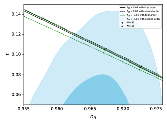
Figure 1: Marginalized constraint (68% and 95% confidence level) from $(n_{\cal R},r)$ using Planck 2018 data, compared to the theoretical predictions of the model with $n=4/3$. For both $f_{\rm{GB}}=0.02$ and $f_{\rm{GB}}=-0.01$, the solid lines give the results with the first-order corrections while the dash gives the predictions with the second-order corrections, respectively.

Considering about the smaller errors on $n_{R}$ and $r$ in the future, the second-order corrections to both $n_{R}$ and $r$ in the slow-roll approximation are important. In the forthcoming experiments, especially the Stage IV experiments CMB-S4:2016ple ; SimonsObservatory:2018koc ; Mallaby-Kay:2021tuk ; LiteBIRD:2022cnt , the errors of the measurements on both $n_{R}$ and $r$ will be smaller than $10^{-3}$, namely $\sigma(n_{\cal R},r)<10^{-3}$. That means it is necessary to calculate the second-order corrections of $n_{\cal R}$ and $r$ to the magnitude of $\mathcal{O}(10^{-3})$ for getting more accurate constraints on the parameters of the models. On this order of magnitude, the first-order and second-order results will be easily distinguished by future experiments. It is worth noting that the contributions of second-order corrections are affected by the parameters of the models.

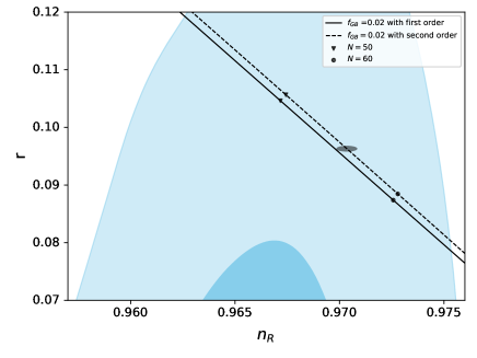
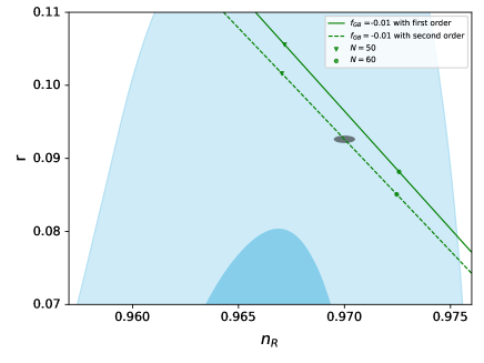
Figure 2: Difference between the $n_{\cal R}-r$ relations with the first- and the second-order corrections. The gray shaded $1-\sigma$ contour corresponds to a futuristic measurement with $\sigma_{n_{s-1}}=\sigma_{r}=10^{-3}$.

In Fig. 2, the first-order and the second-order results of $n_{\cal R}$ and $r$ with Planck 2018 constraints in the models for different values of $N$ and $f_{\rm{GB}}$ are compared. The upper panel in Fig. 2 is for $f_{\rm{GB}}=0.02$, while the bottom panel is for $f_{\rm{GB}}=-0.01$, in which the shaded contour means a possible futuristic measurement with $\sigma(n_{\cal R},r)<10^{-3}$. It is easy to find that for both $f_{\rm{GB}}=0.02$ and $f_{\rm{GB}}=-0.01$, the difference between the first-order and second-order predictions is larger than the futuristic experimental sensitivity on $n_{\cal R}$ and $r$, and this is even more obvious for $f_{\rm{GB}}=-0.01$ . This would make it convincing that the second-order corrections in the slow-roll approximation of $n_{\cal R}$ and $r$ in 4EGB inflation are necessary for fitting future experimental data.

VI Conclusions and Outlook

The uniform asymptotic approximation method is an error-controlled and systematically improvable method for constructing exact analytical solutions of linear perturbations. The effectiveness of this method has been verified in many applications, for example, in calculating primordial spectra for various inflation models Zhu:2013fha ; Zhu:2013upa ; Zhu:2014wfa ; Zhu:2015ata ; Zhu:2016srz ; Zhu:2014wda ; Zhu:2014aea ; Zhu:2015xsa ; Zhu:2015owa and applications in studying the reheating process Zhu:2018smk and quantum mechanics Li:2019cre .

In this paper, we applied the third-order uniform asymptotic approximation to derive the inflationary observables for scalar and tensor perturbations in the slow-roll inflation in the spatial covariant 4EGB gravity. With both scalar and tensor perturbations in terms of the flow of the Hubble flow slow-roll paramaters and the GB coupling constant, we obtained explicitly the analytical expressions of the primordial power spectra, spectral indices, running of spectral indices for both scalar and tensor perturbations, and the ratio between the tensor and scalar spectra up to the second-order in the expansions of the slow-roll approximation. Compared with the results obtained in the previous literature, the results presented in this paper represent the most accurate results obtained so far in the literature.

As we have mentioned in Sec. I, the high-order corrections to the inflationary observables in the slow-roll expansions are very important in the future analysis of different inflation models with precise experimental data. For example, it is pointed out in Martin:2014rqa that the future CMB experiments can measure both $n_{\mathcal{R}}$ and $r$ to be accurate with errors $\gtrsim 10^{-3}$. Thus, the contributions from the GB coupling constant to the scalar spectral index and the tensor-to-scalar ratio in general can not be ignored if they are at the magnitude of $\mathcal{O}(10^{3})$. We expect the more precise forthcoming experimental data in the future can make significant constraint on the GB coupling constant in the spatial covariant 4EGB gravity, which could help us to understand the physics of the early universe.

Appendix A: General formulas of primordial spectra in the uniform asymptotic approximation

In this section, we present a brief introduction of the general formulas of primordial perturbations with a slow-varying sound speed and parameter $b(\tau)$ arsing from the nonlinear dispersion relation.

In the uniform asymptotic approximation, we first write Eqs.(3.21) and (3.33) in the standard form Zhu:2013upa

$$\frac{d^{2}\mu(y)}{dy^{2}}=\{\lambda^{2}\hat{g}(y)+q(y)\}\mu(y),$$ (A.1)

where the new variables $y=-k\tau$, $\mu(y)=\mu_{\mathcal{R}}(y)$ and $\mu_{h}(y)$ correspond to scalar and tensor perturbations respectively, and

$$\lambda^{2}\hat{g}(y)+q(y)=\frac{\nu^{2}(\tau)-1/4}{y^{2}}-c^{2}(\tau)-b(\tau)y^{2}.$$ (A.2)

where $c(\tau)=c_{s,t}(\tau)$ is the effective sound speed for scalar and tensor perturbation modes respectively. For scalar perturbation, we have Aoki:2020iwm

$$\nu_{\mathcal{R}}^{2}(\tau)=\tau^{2}\frac{z^{\prime\prime}(\tau)}{z(\tau)}+\frac{1}{4}\;\;{\rm with}\;\;c(\tau)=1\;\;{\rm and}\;\;b(\tau)=0,$$

and for tensor modes,

$$\nu_{h}^{2}(\tau)=\tau^{2}\frac{a^{\prime\prime}(\tau)}{a(\tau)}+\frac{1}{4}.$$ (A.4)

It’s worth noting that $\lambda$ is an assumed large parameter which is used to label the different approximate orders of the uniform asymptotic approximation, as we will see later in the square bracket of the general formulas of power spectrum in Eq. (Appendix A: General formulas of primordial spectra in the uniform asymptotic approximation) in the square bracket. $\lambda=1$ can be set to $\lambda=1$ for simplicity in the ending calculation. Now we need to use the uniform asymptotic approximation to construct the approximate solutions of the above equation. In order to ensure the convergence of the errors of the approximate solutions, the only option is Zhu:2013upa

$$q(y)=-\frac{1}{4y^{2}}.$$ (A.5)

Then, Eq. (A.2) can be written as

$$\lambda^{2}\hat{g}(y)=\frac{\nu^{2}(\tau)}{y^{2}}-c^{2}(\tau)-b(\tau)y^{2},$$ (A.6)

Here for scalar perturbation, $b(\tau)>0$ must meet the condition $b(\tau)>0$ for a healthy UV limit .

Since $b(\tau)$ is a small quantity, it is easy to find that the function $\lambda^{2}\hat{g}(y)$ has a unique turning point, which is expressed as follows

$$y_{0}^{2}(\bar{\tau}_{0}) = \frac{-c_{0}^{2}(\bar{\tau}_{0})+\sqrt{\bar{c}_{0}^{4}(\tau_{0})+4b(\bar{\tau}_{0})\bar{\nu}_{0}^{2}(\bar{\tau}_{0})}}{2b(\bar{\tau}_{0})}.$$ (A.7)

Then with reference to Zhu:2014wfa , the general formula of the power spectrum can be written as follows

$$\Delta^{2}(k) \equiv \frac{k^{3}}{4\pi^{2}}\left|\frac{u(y)}{z(\tau)}\right|^{2}_{y\to 0^{+}}$$

$$= \frac{k^{2}}{8\pi^{2}}\frac{-k\tau}{z^{2}(\tau)\nu(\tau)}\exp{\left(2\lambda\int_{y}^{\bar{y}_{0}}\sqrt{\hat{g}(y^{\prime})}dy^{\prime}\right)}$$

$$\times\left[1+\frac{\mathscr{H}(+\infty)}{\lambda}+\frac{\mathscr{H}^{2}(+\infty)}{2\lambda^{2}}+\mathcal{O}\left(\frac{1}{\lambda^{3}}\right)\right].$$

The order of the parameter $\lambda$ shows that the formula is in third order approximation. The integral of $\sqrt{g}$ in this formulas is given by Eqs. (B.9) where $I_{0}$ and $I_{1}$ are given by Eqs. (B.10) and (B.11), and the error control function is given by (B.13).

Then we need to calculate the spectral indices. For this purpose, we primarily specify the $k$-dependence of $\bar{\nu}_{0}(\tau_{0})$, $\bar{\nu}_{1}(\tau_{0})$ through $\tau_{0}=\tau_{0}(k)$. From the relation $-k\tau_{0}=\bar{y}_{0}$, we obtain

$$\frac{d\ln(-\tau_{0})}{d\ln k} = -1+\frac{d\ln\bar{y}_{0}}{d\ln(-\tau_{0})}\frac{d\ln(-\tau_{0})}{d\ln k},$$ (A.9)

which approximation is

$$\frac{d\ln(-\tau_{0})}{d\ln k} \simeq -1-\frac{d\ln\bar{y}_{0}}{d\ln(-\tau_{0})}.$$ (A.10)

Then with this relation, the spectral index can be written as

$$n_{\mathcal{R}}-1,\;n_{h} \equiv \frac{d\ln\Delta^{2}_{s,t}}{d\ln k}$$ (A.11)

$$\simeq 3-2\bar{\nu}_{0}-\frac{2\bar{b}_{1}\bar{\nu}_{0}}{3\bar{c}_{0}^{4}}+\frac{2\bar{c}_{1}\bar{\nu}_{0}}{\bar{c}_{0}}+\frac{2\bar{b}_{1}\bar{\nu}_{0}^{3}}{3\bar{c}_{0}^{4}}$$

$$-2\bar{\nu}_{1}\ln 2+\frac{\bar{\nu}_{1}}{6\bar{\nu}_{0}^{2}}.$$

The running of the spectral index $\alpha\equiv dn/d\ln k$ can be similarly written as

$$\alpha_{\mathcal{R},\;h}(k) \simeq 2\bar{\nu}_{1}+\frac{2\bar{b}_{2}\bar{\nu}_{0}}{3\bar{c}_{0}^{4}}-\frac{2\bar{c}_{2}\bar{\nu}_{0}}{\bar{c}_{0}}-\frac{2\bar{b}_{2}\bar{\nu}_{0}^{3}}{3\bar{c}_{0}^{4}}$$ (A.12)

$$+2\bar{\nu}_{2}\ln 2-\frac{\bar{\nu}_{2}}{6\bar{\nu}_{0}^{2}}.$$

In the above, all the formulas (Eqs.(Appendix A: General formulas of primordial spectra in the uniform asymptotic approximation), (A.11), and (A.12)) can be used to calculate the primordial perturbation spectra with different inflation models. It is easy to use these formulas, because they are determined only by the quantities $H(\tau)$, ($c_{0},c_{1},c_{2}$), ($\nu_{0},\nu_{1},\nu_{2}$) which are evaluated at the turning point. And these quantities can be easily obtain from Eqs. (3.22, Appendix A: General formulas of primordial spectra in the uniform asymptotic approximation) for scalar perturbations and Eqs. (3.34, A.4) for tensor perturbations. In section IV, we apply these formulas to calculate the slow-roll power spectra for both scalar and tensor perturbations in the spatial covariant 4EGB gravity.

Appendix B: Integrals of $\sqrt{g}$ and the error control function

From Eq.(A.6) with $\lambda=1$, we have

$$g(y)=\frac{\nu^{2}(\tau)}{y^{2}}-c^{2}(\tau)-b(\tau)y^{2}.$$ (B.1)

where

$$\nu(\tau)\simeq\bar{\nu}_{0}+\bar{\nu}_{1}\ln\frac{y}{\bar{y}_{0}}+\bar{\nu}_{2}\ln^{2}\frac{y}{\bar{y}_{0}},$$ (B.2)

$$c(\tau)\simeq\bar{c}_{0}+\bar{c}_{1}\ln\frac{y}{\bar{y}_{0}}+\bar{c}_{2}\ln^{2}\frac{y}{\bar{y}_{0}},$$ (B.3)

$$b(\tau)\simeq\bar{b}_{0}+\bar{b}_{1}\ln\frac{y}{\bar{y}_{0}}+\bar{b}_{2}\ln^{2}\frac{y}{\bar{y}_{0}}.$$ (B.4)

with

$$\bar{\nu}_{1} \equiv \frac{d\nu(\tau)}{d\ln(-\tau)}\Big{|}_{\tau_{0}},\bar{\nu}_{2}\equiv\frac{d^{2}\nu(\tau)}{d\ln^{2}(-\tau)}\Big{|}_{\tau_{0}},$$ (B.5)

$$\bar{c}_{1} \equiv \frac{dc(\tau)}{d\ln(-\tau)}\Big{|}_{\tau_{0}},\bar{c}_{2}\equiv\frac{d^{2}c(\tau)}{d\ln^{2}(-\tau)}\Big{|}_{\tau_{0}},$$ (B.6)

$$\bar{b}_{1} \equiv \frac{db(\tau)}{d\ln(-\tau)}\Big{|}_{\tau_{0}},\bar{b}_{2}\equiv\frac{d^{2}b(\tau)}{d\ln^{2}(-\tau)}\Big{|}_{\tau_{0}}.$$ (B.7)

Substitute Eqs.(B.2), (B.3) and (B.4) into Eq.(B.1), we have

$$\sqrt{g(y)}= \frac{\sqrt{\bar{\nu}_{0}^{2}-\bar{c}_{0}^{2}y^{2}-\bar{b}_{0}y^{4}}}{y}$$ (B.8)

$$+ \frac{2\bar{\nu}_{0}\bar{\nu}_{1}-2\bar{c}_{0}\bar{c}_{1}y^{2}-b_{1}y^{4}}{2y\sqrt{\bar{\nu}_{0}^{2}-\bar{c}_{0}^{2}y^{2}-\bar{b}_{0}y^{4}}}\ln\frac{y}{\bar{y}_{0}}.$$

Then we divided the integral $\int\sqrt{g(y)}dy$ into two parts,

$$\int_{y}^{\bar{y}_{0}}\sqrt{g(y)}dy\simeq I_{0}+I_{1},$$ (B.9)

where

$$\lim_{y\rightarrow 0}I_{0} \simeq -\frac{\bar{\nu}_{0}}{2}-\frac{\bar{c}_{0}^{2}}{4\sqrt{\bar{b}_{0}}}\arctan\Big{(}\frac{2\sqrt{\bar{b}_{0}}\bar{\nu}_{0}}{\bar{c}_{0}^{2}}\Big{)}$$ (B.10)

$$-\frac{1}{4}\bar{\nu}_{0}\ln(\bar{c}_{0}^{4}+4\bar{b}_{0}\bar{\nu}_{0}^{2})-\bar{\nu}_{0}\ln\frac{y}{2\bar{\nu}_{0}},$$

$$\lim_{y\rightarrow 0}I_{1} \simeq \bar{b}_{1}\bar{\nu}_{0}^{3}\frac{5-6\ln{2}}{18\bar{c}_{0}^{4}}+\bar{\nu}_{0}\bar{c}_{1}\frac{1-\ln{2}}{\bar{c}_{0}}$$ (B.11)

$$+\bar{\nu}_{1}\Big{(}-\frac{\pi^{2}}{24}+\frac{\ln^{2}2}{2}-\frac{1}{2}\ln^{2}\frac{y}{\bar{y}_{0}}\Big{)}.$$

The integral form of error control function is

$$\mathscr{H}(\xi) \simeq \frac{5}{36}\Big{\{}\int_{\bar{y}_{0}}^{y}\sqrt{g{y}dy}\Big{\}}^{-1}\Big{|}_{\bar{y}_{0}}^{y}$$ (B.12)

$$-\int_{\bar{y}_{0}}^{y}\Big{\{}\frac{q}{g}-\frac{5{g^{\prime}}^{2}}{16g^{3}}+\frac{g^{\prime\prime}}{4g^{2}}\Big{\}}\sqrt{g}dy.$$

When $y\rightarrow 0$, the error control function can be written as

$$\mathscr{H}(+\infty) \simeq \frac{\bar{c}_{0}^{4}+8\bar{b}_{0}\bar{\nu}_{0}^{2}}{6\bar{c}_{0}^{4}\bar{\nu}_{0}+24\bar{b}_{0}\bar{\nu}_{0}^{3}}$$ (B.13)

$$+\frac{\bar{c}_{1}}{6\bar{c}_{0}\bar{\nu}_{0}}-\frac{23+12\ln{2}}{72\bar{\nu}_{0}^{2}}\bar{\nu}_{1}$$

$$+\frac{(1+4\ln{2})\bar{\nu}_{0}}{6\bar{c}_{0}}\bar{b}_{1}.$$

References

- (1) A. H. Guth, “The Inflationary Universe: A Possible Solution to the Horizon and Flatness Problems,” Phys. Rev. D 23, 347-356 (1981).
- (2) A. A. Starobinsky, “A New Type of Isotropic Cosmological Models Without Singularity,” Phys. Lett. B 91, 99-102 (1980).
- (3) K. Sato, “First Order Phase Transition of a Vacuum and Expansion of the Universe,” Mon. Not. Roy. Astron. Soc. 195, 467-479 (1981).
- (4) D. Baumann, “Inflation,” [arXiv:0907.5424 [hep-th]].
- (5) E. Komatsu et al. [WMAP], “Seven-Year Wilkinson Microwave Anisotropy Probe (WMAP) Observations: Cosmological Interpretation,” Astrophys. J. Suppl. 192 , 18(2011) [arXiv:1001.4538 [astro-ph.CO]].
- (6) D. Larson, J. Dunkley, G. Hinshaw, E. Komatsu, M. R. Nolta, C. L. Bennett, B. Gold, M. Halpern, R. S. Hill and N. Jarosik, et al. “Seven-Year Wilkinson Microwave Anisotropy Probe (WMAP) Observations: Power Spectra and WMAP-Derived Parameters,” Astrophys. J. Suppl. 192 , 16(2011) [arXiv:1001.4635 [astro-ph.CO]].
- (7) P. A. R. Ade et al. [Planck], “Planck 2015 results. XX. Constraints on inflation,” Astron. Astrophys. 594 , A20(2016) [arXiv:1502.02114 [astro-ph.CO]].
- (8) P. A. R. Ade et al. [Planck], “Planck 2015 results. XVII. Constraints on primordial non-Gaussianity,” Astron. Astrophys. 594 , A17(2016) [arXiv:1502.01592 [astro-ph.CO]].
- (9) J. Martin and R. H. Brandenberger, “The TransPlanckian problem of inflationary cosmology,” Phys. Rev. D 63 , 123501(2001) [arXiv:hep-th/0005209 [hep-th]].
- (10) R. H. Brandenberger and J. Martin, “Trans-Planckian Issues for Inflationary Cosmology,” Class. Quant. Grav. 30 , 113001(2013) [arXiv:1211.6753 [astro-ph.CO]].
- (11) A. Borde and A. Vilenkin, “Eternal inflation and the initial singularity,” Phys. Rev. Lett. 72 , 3305-3309(1994) [arXiv:gr-qc/9312022 [gr-qc]].
- (12) A. Borde, A. H. Guth and A. Vilenkin, “Inflationary space-times are incompletein past directions,” Phys. Rev. Lett. 90 , 151301(2003) [arXiv:gr-qc/0110012 [gr-qc]].
- (13) A. Wang, “Hořava gravity at a Lifshitz point: A progress report,” Int. J. Mod. Phys. D 26, 1730014(2017) [arXiv:1701.06087 [gr-qc]].
- (14) D. Baumann and L. McAllister, “Inflation and String Theory,” Cambridge University Press, 2015, ISBN 978-1-107-08969-3, 978-1-316-23718-2 [arXiv:1404.2601 [hep-th]].
- (15) D. Glavan and C. Lin, “Einstein-Gauss-Bonnet Gravity in Four-Dimensional Spacetime,” Phys. Rev. Lett. 124, no.8, 081301 (2020) [arXiv:1905.03601 [gr-qc]].
- (16) R. A. Hennigar, D. Kubizňák, R. B. Mann and C. Pollack, “On taking the D → 4 limit of Gauss-Bonnet gravity: theory and solutions,” JHEP 07, 027 (2020) [arXiv:2004.09472 [gr-qc]].
- (17) P. G. S. Fernandes, P. Carrilho, T. Clifton and D. J. Mulryne, “Derivation of Regularized Field Equations for the Einstein-Gauss-Bonnet Theory in Four Dimensions,” Phys. Rev. D 102, no.2, 024025 (2020) [arXiv:2004.08362 [gr-qc]].
- (18) W. Y. Ai, “A note on the novel 4D Einstein–Gauss–Bonnet gravity,” Commun. Theor. Phys. 72, no.9, 095402(2020) [arXiv:2004.02858 [gr-qc]].
- (19) M. Gürses, T. Ç. Şişman and B. Tekin, “Is there a novel Einstein–Gauss–Bonnet theory in four dimensions?,” Eur. Phys. J. C 80, no.7, 647 (2020) [arXiv:2004.03390 [gr-qc]].
- (20) F. W. Shu, “Vacua in novel 4D Einstein-Gauss-Bonnet Gravity: pathology and instability?,” Phys. Lett. B 811, 135907 (2020) [arXiv:2004.09339 [gr-qc]].
- (21) H. Lu and Y. Pang, “Horndeski gravity as limit of Gauss-Bonnet,” Phys. Lett. B 809, 135717 (2020) [arXiv:2003.11552 [gr-qc]].
- (22) T. Kobayashi, “Effective scalar-tensor description of regularized Lovelock gravity in four dimensions,” JCAP 07 , 013(2020) [arXiv:2003.12771 [gr-qc]].
- (23) J. Bonifacio, K. Hinterbichler and L. A. Johnson, “Amplitudes and 4D Gauss-Bonnet Theory,” Phys. Rev. D 102, no.2, 024029 (2020) [arXiv:2004.10716 [hep-th]].
- (24) S. Mahapatra, Eur. Phys. J. C 80, no.10, 992 (2020) doi:10.1140/epjc/s10052-020-08568-6 [arXiv:2004.09214 [gr-qc]].
- (25) P. X. Jiang, J. W. Hu and Z. K. Guo, “Inflation coupled to a Gauss-Bonnet term,” Phys. Rev. D 88 , 123508(2013) [arXiv:1310.5579 [hep-th]].
- (26) Z. K. Guo and D. J. Schwarz, “Slow-roll inflation with a Gauss-Bonnet correction,” Phys. Rev. D 81, 123520 (2010) [arXiv:1001.1897 [hep-th]].
- (27) S. Koh, B. H. Lee, W. Lee and G. Tumurtushaa, “Observational constraints on slow-roll inflation coupled to a Gauss-Bonnet term,” Phys. Rev. D 90, no.6, 063527 (2014) [arXiv:1404.6096 [gr-qc]].
- (28) M. Satoh, “Slow-roll Inflation with the Gauss-Bonnet and Chern-Simons Corrections,” JCAP 11, 024 (2010) [arXiv:1008.2724 [astro-ph.CO]].
- (29) M. Satoh and J. Soda, “Higher Curvature Corrections to Primordial Fluctuations in Slow-roll Inflation,” JCAP 09, 019 (2008) [arXiv:0806.4594 [astro-ph]].
- (30) C. van de Bruck and C. Longden, “Higgs Inflation with a Gauss-Bonnet term in the Jordan Frame,” Phys. Rev. D 93, no.6, 063519 (2016) [arXiv:1512.04768 [hep-ph]].
- (31) M. Satoh, S. Kanno and J. Soda, “Circular Polarization of Primordial Gravitational Waves in String-inspired Inflationary Cosmology,” Phys. Rev. D 77, 023526 (2008) [arXiv:0706.3585 [astro-ph]].
- (32) S. Chakraborty, T. Paul and S. SenGupta, “Inflation driven by Einstein-Gauss-Bonnet gravity,” Phys. Rev. D 98, no.8, 083539 (2018) [arXiv:1804.03004 [gr-qc]].
- (33) K. Aoki, M. A. Gorji, S. Mizuno and S. Mukohyama, “Inflationary gravitational waves in consistent Einstein-Gauss-Bonnet gravity,” JCAP 01, 054 (2021) [arXiv:2010.03973 [gr-qc]].
- (34) K. N. Abazajian et al. [CMB-S4], “CMB-S4 Science Book, First Edition,” [arXiv:1610.02743 [astro-ph.CO]].
- (35) P. Ade et al. [Simons Observatory], “The Simons Observatory: Science goals and forecasts,” JCAP 02, 056 (2019) [arXiv:1808.07445 [astro-ph.CO]].
- (36) M. Mallaby-Kay, Z. Atkins, S. Aiola, S. Amodeo, J. E. Austermann, J. A. Beall, D. T. Becker, J. R. Bond, E. Calabrese and G. E. Chesmore, et al. “The Atacama Cosmology Telescope: Summary of DR4 and DR5 Data Products and Data Access,” Astrophys. J. Supp. 255 , no.1, 11(2021) [arXiv:2103.03154 [astro-ph.CO]].
- (37) E. Allys et al. [LiteBIRD], “Probing Cosmic Inflation with the LiteBIRD Cosmic Microwave Background Polarization Survey,” [arXiv:2202.02773 [astro-ph.IM]].
- (38) P. A. Abell et al. [LSST Science and LSST Project], “LSST Science Book, Version 2.0,” [arXiv:0912.0201 [astro-ph.IM]].
- (39) F. Lacasa, “Cosmology in the non-linear regime: the small scale miracle,” Astron. Astrophys. 661, A70 (2022) [arXiv:1912.06906 [astro-ph.CO]].
- (40) S. Ilić et al. [Euclid], “Euclid preparation - XV. Forecasting cosmological constraints for the Euclid and CMB joint analysis,” Astron. Astrophys. 657, A91 (2022) [arXiv:2106.08346 [astro-ph.CO]].
- (41) P. Adshead, R. Easther, J. Pritchard and A. Loeb, “Inflation and the Scale Dependent Spectral Index: Prospects and Strategies,” JCAP 02, 021 (2011) [arXiv:1007.3748 [astro-ph.CO]].
- (42) J. Martin, C. Ringeval and V. Vennin, “How Well Can Future CMB Missions Constrain Cosmic Inflation?,” JCAP 10, 038 (2014) [arXiv:1407.4034 [astro-ph.CO]].
- (43) T. Sprenger, M. Archidiacono, T. Brinckmann, S. Clesse and J. Lesgourgues, “Cosmology in the era of Euclid and the Square Kilometre Array,” JCAP 02, 047 (2019) [arXiv:1801.08331 [astro-ph.CO]].
- (44) K. Aoki, M. A. Gorji and S. Mukohyama, “A consistent theory of Einstein-Gauss-Bonnet gravity,” Phys. Lett. B 810, 135843 (2020) [arXiv:2005.03859 [gr-qc]].
- (45) T. Zhu, A. Wang, G. Cleaver, K. Kirsten and Q. Sheng, “Constructing analytical solutions of linear perturbations of inflation with modified dispersion relations,” Int. J. Mod. Phys. A 29, no.23, 1450142 (2014) [arXiv:1308.1104 [astro-ph.CO]].
- (46) T. Zhu, A. Wang, G. Cleaver, K. Kirsten and Q. Sheng, “Inflationary cosmology with nonlinear dispersion relations,” Phys. Rev. D 89, no.4, 043507 (2014) [arXiv:1308.5708 [astro-ph.CO]].
- (47) T. Zhu, A. Wang, G. Cleaver, K. Kirsten and Q. Sheng, “Power spectra and spectral indices of -inflation: high-order corrections,” Phys. Rev. D 90, no.10, 103517 (2014) [arXiv:1407.8011 [astro-ph.CO]].
- (48) T. Zhu, A. Wang, K. Kirsten, G. Cleaver, Q. Sheng and Q. Wu, “Inflationary spectra with inverse-volume corrections in loop quantum cosmology and their observational constraints from Planck 2015 data,” JCAP 03, 046 (2016) [arXiv:1510.03855 [gr-qc]].
- (49) T. Zhu, Q. Wu and A. Wang, “An analytical approach to the field amplification and particle production by parametric resonance during inflation and reheating,” Phys. Dark Univ. 26, 100373 (2019) [arXiv:1811.12612 [hep-ph]].
- (50) T. Zhu, A. Wang, K. Kirsten, G. Cleaver and Q. Sheng, “High-order Primordial Perturbations with Quantum Gravitational Effects,” Phys. Rev. D 93, no.12, 123525 (2016) [arXiv:1604.05739 [gr-qc]].
- (51) T. Zhu and A. Wang, “Gravitational quantum effects in light of BICEP2 results,” Phys. Rev. D 90, no.2, 027304 (2014) [arXiv:1403.7696 [astro-ph.CO]].
- (52) T. Zhu, A. Wang, G. Cleaver, K. Kirsten and Q. Sheng, “Gravitational quantum effects on power spectra and spectral indices with higher-order corrections,” Phys. Rev. D 90, no.6, 063503 (2014) [arXiv:1405.5301 [astro-ph.CO]].
- (53) T. Zhu, A. Wang, G. Cleaver, K. Kirsten, Q. Sheng and Q. Wu, “Detecting quantum gravitational effects of loop quantum cosmology in the early universe?,” Astrophys. J. Lett. 807, no.1, L17 (2015) [arXiv:1503.06761 [gr-qc]].
- (54) T. Zhu, A. Wang, G. Cleaver, K. Kirsten, Q. Sheng and Q. Wu, “Scalar and tensor perturbations in loop quantum cosmology: High-order corrections,” JCAP 10, 052 (2015) [arXiv:1508.03239 [gr-qc]].
- (55) N. Aghanim et al. [Planck], “Planck 2018 results. VI. Cosmological parameters,” Astron. Astrophys. 641, A6 (2020) [erratum: Astron. Astrophys. 652, C4 (2021)] [arXiv:1807.06209 [astro-ph.CO]].
- (56) K. Aoki, M. A. Gorji and S. Mukohyama, “Cosmology and gravitational waves in consistent Einstein-Gauss-Bonnet gravity,” JCAP 09 , 014(2020) [erratum: JCAP 05, E01 (2021)] [arXiv:2005.08428 [gr-qc]].
- (57) B. F. Li, T. Zhu and A. Wang, “Langer Modification, Quantization condition and Barrier Penetration in Quantum Mechanics,” Universe 6, 90 (2020) [arXiv:1902.09675 [quant-ph]].
- (58) P. Auclair and C. Ringeval, “Slow-roll inflation at N3LO,” Phys. Rev. D 106, 063512 (2022) [arXiv:2205.12608 [astro-ph.CO]].
- (59) J. Martin, C. Ringeval, and V. Vennin, Shortcomings of new parametrizations of inflation, Phys. Rev. D 94, 123521 (2016).
- (60) J. Martin, C. Ringeval, and V. Vennin, Encyclopdia Inflationaris, Phys. Dark Universe 5–6, 75 (2014).