Robust Saliency Guidance for Data-free Class Incremental Learning

Abstract

Data-Free Class Incremental Learning (DFCIL) aims to sequentially learn tasks with access only to data from the current one. DFCIL is of interest because it mitigates concerns about privacy and long-term storage of data, while at the same time alleviating the problem of catastrophic forgetting in incremental learning. In this work, we introduce robust saliency guidance for DFCIL and propose a new framework, which we call RObust Saliency Supervision (ROSS), for mitigating the negative effect of saliency drift. Firstly, we use a teacher-student architecture leveraging low-level tasks to supervise the model with global saliency. We also apply boundary-guided saliency to protect it from drifting across object boundaries at intermediate layers. Finally, we introduce a module for injecting and recovering saliency noise to increase robustness of saliency preservation. Our experiments demonstrate that our method can retain better saliency maps across tasks and achieve state-of-the-art results on the CIFAR-100, Tiny-ImageNet and ImageNet-Subset DFCIL benchmarks. Code will be made publicly available.

1 Introduction

Deep neural networks achieve state-of-the-art performance on many computer vision tasks. However, most of these tasks consider a static world in which tasks are well-defined, stationary, and all training data is available in a single training session. The real world consists of dynamically changing environments and data distributions, which – especially given the computational burden of training large CNNs – has led to renewed interest learning new tasks incrementally while avoiding catastrophic forgetting of old ones [27, 11].

Class Incremental Learning (CIL) [26, 1] is a scenario that considers the possibility of adding new classes to already-trained models. Most CIL methods rely on a memory buffer that stores data from past tasks [29, 2, 9, 33]. In this paper, we consider Data-Free Class Incremental Learning (DFCIL), which is a more challenging scenario in which no data from previous tasks is retained. This is a realistic scenario and of great interest due to privacy concerns or restrictions on long-term storage of data. The inability to retain examples from past tasks, however, significantly exacerbates the problem of catastrophic forgetting.

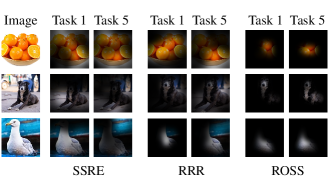
Figure 1: Illustration of saliency drift across 5 tasks on ImageNet-Subset. SSRE [43] is a representative method without saliency supervision which results in random saliency drift toward the background. RRR [10] vanilla saliency supervision method which however fails to avoid saliency drift across boundary regions. These phenomena lead to incorrect predictions: Orange to Bowl, Dog to Shoe, Bird to Boat. In comparison, ROSS maintains robust saliency and preventing saliency drift across boundaries.

There are several recent works that consider the DFCIL problem. DeepInversion [37] inverts trained networks from random noise to generate images as exemplars mixed with current samples for training. SDC [38] updates previous prototypes of each learned class by hypothesizing that semantic drift of previous classes can be approximated and estimated using new data. Other previous works propose representation learning methods for overcoming catastrophic forgetting [41, 42]. As pointed out in IL2A [41], learning better representations can reduce representation bias when transferred to new tasks. Incorporating self-supervised learning tasks, such as Barlow Twins [28] and rotation prediction [42], has also been proposed to achieve more stable representations and alleviate forgetting.

CNNs naturally learn to attend to features that are discriminative for the tasks they are trained to solve. Catastrophic forgetting also occurs in DFCIL due to that model’s attention to salient features drifting to features specific to the new task. Standard regularization approaches do little to prevent this saliency drift when learning new tasks. One direct method of regularizing saliency is to apply distillation on saliency maps of old samples [10]. However, this is complicated by the inability to save samples from previous tasks in the DFCIL setting. Another method is to apply saliency distillation between current task samples and previous task attention [8]. This method however suffers from the semantic gap between current and old classes when enforcing saliency consistency. A lack of robust saliency regularization may also lead to attention drifting toward the background in future tasks. As demonstrated in Table 1, a conventional baseline (e.g. SSRE [42]) results in random saliency drift toward the background, and vanilla saliency supervision (e.g. RRR [10]) fails to avoid saliency drift across boundary regions in future tasks. Our Robust Saliency Supervision (ROSS) approach, however, keeps saliency focused on the foreground across incrementally learned tasks (for more details, see Section 4).

Motivated by these observations, we propose the Robust Saliency Supervision (ROSS) approach which incorporates three components to address this problem. ROSS first uses a teacher-student architecture in which the teacher model provides low-level supervision of salient regions and salient region boundary maps. This serves as a stationary supervision signal over the incremental model. Additionally, we apply dilated boundary maps to avoid saliency drift across object boundaries at intermediate layers in the CNNs. Since saliency drift usually happens across tasks, encouraging the model to focus on important foreground regions with dilated boundary supervision reduces the likelihood of saliency shifting toward the background. Finally, inspired by SDC [38], we propose a module to inject saliency noise into some feature channels and train the network to denoise them. This helps the network further resist saliency drift across tasks.

The main contributions of this work are: (i) We provide new insight into robust saliency supervision under DFCIL settings; we also show the negative effect of methods with no or trivial saliency supervision, which illustrates the superiority of our method and motivates the need for saliency drift mitigation in DFCIL. (ii) We propose the Robust Saliency Supervision (ROSS) framework with three components that combine to mitigate the saliency drift problem. (iii) We show that ROSS can be easily integrated it into other state-of-the-art methods, such as MUC [23], IL2A [41], PASS [42], SSRE [43], leading to significant performance gains. (iv) Our experiments demonstrate that ROSS outperforms all existing DFCIL methods and even several exemplar-based methods on the CIFAR-100, Tiny-ImageNet, and ImageNet-Subset DFCIL benchmarks.

2 Related Work

We first discuss previous work on incremental learning from the recent literature and then describe work on DFCIL.

2.1 Incremental Learning

A variety of methods have been proposed for incremental learning in the past few years [6, 1]. Recent works can be coarsely grouped into three categories: replay-based, regularization-based, and parameter-isolation methods. Replay-based methods mitigate the task-recency bias by retaining training samples from previous tasks. In addition to replaying samples, BiC [33], PODNet [9], and iCaRL [29] apply a distillation loss to prevent forgetting and enhance model stability. GEM [24], AGEM [3], and MER [30] exploit past-task exemplars by modifying gradients on current training samples to match old samples. Rehearsal-based methods may cause models to overfit to stored samples. Regularization-based approaches such as LwF [20], EWC [15], and DMC [39] offer ways to learn better representations while leaving enough plasticity for adaptation to new tasks. Parameter-isolation methods [25, 34] use models with different computational graphs for each task. With the help of growing models, new model branches mitigate catastrophic forgetting at the cost of more parameters and computational cost.

As for saliency-guided incremental learning, LwM [8] regularizes the saliency activation of previous classes on current task data. However, there exist semantic gaps between current classes and old ones, which results in an inaccurate distillation target for preserving saliency activations on old samples. RRR [10] directly saves the old saliency activation of each sample with Grad-CAM in a replay buffer and applies distillation to memorize this old knowledge, which requires storeing additional samples during incremental learning. Despite these initial works on saliency-guided incremental learning, saliency drift still remains problematic and leads to catastrophic forgetting.

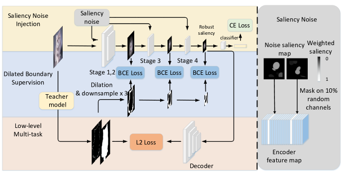
Figure 2: Overall framework of our Robust Saliency Supervision (ROSS). We apply a teacher model to generate saliency and boundary maps. The boundary map is dilated and downsampled to provide supervision at different stages of the encoder. A decoder is attached after the encoder for low-level distillation, which serves as the robust teacher saliency guidance. To prevent saliency drift in later training phases, we introduce saliency noise into each encoder stage. The model is trained to denoise and reduce the saliency drift on testing current data in future phases. ROSS can be integrated into a DFCIL approach to provide robust saliency guidance across incremental tasks.

2.2 Data-free Class Incremental Learning

Compared to conventional class incremental learning, data-free class incremental learning is more appropriate for applications where training data is sensitive and may not be stored in perpetuity. DAFL [4] uses a GAN to generate synthetic samples from past tasks as an alternative to storing actual data. DeepInversion, which inverts trained networks using random noise to generate images, is another popular DFCIL method [37]. Always Be Dreaming further improves on DeepInversion for DFCIL [32]. SDC attempts to overcome the problems caused by semantic drift when training new tasks on old class samples [38]. It directly estimates prototypes of each learned class to use in a nearest class mean classifier. PASS [42] and IL2A [41] are prototype-based replay methods for efficient and effective DFCIL. Both introduce an efficient way of generating prototypes of old classes. Since these prototypes are features computed from past training samples, original images need not be retained. SSRE [43] introduces a re-parameterization method to trade-off between old and new knowledge. Our Robust Saliency Supervision (ROSS) method uses three three new components to reduce saliency drift in DFCIL and is complementary to several of the approaches mentioned above.

3 Robust Saliency Supervision for DFCIL

We first define the Data-free Class Incremental Learning (DFCIL) scenario and our framework for low-level saliency supervision. Then we describe our approach to dilated boundary supervision and saliency noise injection that further mitigate saliency drift in DFCIL. Our overall framework is illustrated in Figure 2.

3.1 Data-Free Class-Incremental Learning

Class-incremental learning aims to sequentially learn tasks consisting of disjoint classes of samples. Let $t\in\{1,2,..T\}$ denote the incremental learning tasks. The training data $D_{t}$ for each task contains classes $C_{t}$ with $N_{t}$ training samples $\{(x_{t}^{i},y_{t}^{i})\}_{i=1}^{N_{t}}$, where $x^{i}_{t}$ are images and $y_{t}^{i}\in C_{t}$ are their labels.

Most deep networks applied to class-incremental learning can be split into two components: a feature extractor $F_{\theta}$ and a common classifier $G_{\phi}$ which grows with each new task $t+1$ to include classes $C_{t+1}$. The feature extractor $F_{\theta}$ first maps the input $x$ to a deep feature vector $z=F_{\theta}(x)\in\mathbb{R}^{d}$, and then the unified classifier $G_{\phi}(z)\in\mathbb{R}^{|C_{t}|}$ is a probability distribution over classes $C_{t}$ that is used to make predictions on input $x$.

Class-incremental learning requires that the model be capable of correctly classifying all samples from previous tasks at any training task – that is, when learning task $t$, the model must not forget how to classify samples from classes from tasks $t^{\prime}<t$. Data-free class-incremental learning additionally restricts models to learn each new task without access to samples from previous ones. This typically leads to learning objectives that minimize a loss function $\mathcal{L}$ defined on current training data $D_{t}$:

$$\mathcal{L}_{t}^{\text{CIL}}(x,y) =\mathcal{L}_{\text{ce}}(G_{\phi_{t}}(F_{\theta_{t}}(x)),y)+\mathcal{L}^{\text{method}}_{t},$$ (1)

where $\mathcal{L}_{\text{ce}}$ is the standard cross-entropy classification loss and $L^{\text{method}}_{t}$ is a method-specific loss that mitigates forgetting of past tasks when learning current task $t$.

3.2 Auxiliary Low-level Supervisions for DFCIL

We propose to learn stable features from low-level stationary tasks shared across all incremental tasks during class-incremental learning. Low-level vision tasks like salient object detection require useful representations of input images. By learning these feature representations across tasks, the model can focus on key area of input images and exploit learned, stable features with less representation drift since the low-level features change very little between tasks.

Saliency map prediction is relevant to image classification since the foreground largely determines the results, while the background is comparatively less important. When learning new tasks with new classes, the background of images of new classes may contain new visual concepts that introduce undesirable noise and lead to forgetting essential previous knowledge. The effectiveness of saliency features for learning classification tasks was demonstrated by Saliency Guided Training [14]. Additional supervision of salient region boundaries can aid salient object detection tasks for both segmentation and localization [40]. The positive interaction between these two tasks brings richer attention to features relevant to the main classification task. It can provide positive guidance in the form of stationary knowledge across class-incremental tasks. Some examples are illustrated in Figure 5.

We incorporate low-level vision tasks into the network using a teacher-student model. A teacher model generates low-level representations of each input image $x$ (saliency and boundary maps in our experiments). We use CSNet [5] to generate saliency and boundary maps, as it is lightweight and efficient, but any low-level model producing saliency maps can be used in our framework. The boundary map is computed with a Laplacian filter over the estimated saliency map. We add a decoder $D_{\psi}$ [18] after the backbone $F_{\theta}$ to predict low-level saliency and boundary maps for input images. The average L2 distance between the student and teacher maps is used as a low-level distillation loss:

$$\mathcal{L}^{\text{lm}}_{t}(x) =\frac{||D_{\psi}(F_{\theta}(x))-A(x)||_{2}}{\sqrt{N}},$$ (2)

where $A(x)$ denotes the output of the teacher network on input $x$, consisting of a saliency map $A_{s}(x)$ and a boundary map $A_{b}(x)$. $D_{\psi}((F_{\theta}(x))$ are combined saliency and boundary maps produced by the decoder, and $N$ is the number of pixels in the student and teacher saliency maps.

3.3 Boundary-guided Mid-level Saliency Drift Regularization

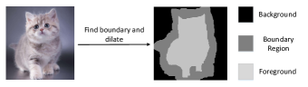
Figure 3: We dilate the teacher boundary map and apply a binary cross entropy loss at three stages in the CNN backbone to prevent mid-level student attention from drifting into boundary regions.

The multi-task supervision of salient regions and boundaries described in the previous section encourages the network to learn representations sufficient to reconstruct the teacher outputs. However, it does little to guide attention at intermediate layers in the CNN. To guard against saliency drift at these intermediate layers in the backbone, we use the generated boundary maps as a type of adaptive supervision as shown in Figure 3. When applying dilated boundary supervision, we add a penalty term on object boundaries to avoid drift into the background. We first use 0.5 as the threshold to binarize the teacher boundary map and then obtain dilated teacher boundary maps by:

$$B_{d}(x) =\text{Dilate}(A_{b}(x),d)$$ (3)

where $A_{b}(x)$ is the original teacher boundary map of image $x$, which is generated from the saliency map a Laplacian filter, and $d$ denotes the dilation radius applied on the teacher boundary map for controlling the strictness of boundary-guided saliency.

Rather than use a decoder at each layer as described above, the student saliency map is generated using Grad-CAM [31] at three stages of the CNN backbone (see Figure 2). We also experiment with several other methods for generating student saliency maps and report these results in the Supplementary Material. The dilated teacher boundary map $B_{d}(x)$ is downsampled to match the feature map dimensions at these three stages in order to compare the Grad-CAM generated saliency boundary maps with the teacher. We use the binary cross entropy loss for supervision on dilated boundary regions. The loss is defined as:

$$\mathcal{L}^{\text{dbs}}_{t}(x) =-\frac{\sum_{j=1}^{N}B_{d}(x,j)\log(1-S(x,j))}{\sum_{j=1}^{N}B_{d}(x,j)},$$ (4)

where $S(x,j)$ denotes the student saliency map of image $x$ at pixel $j$, $B_{d}(x,j)$ is the dilated teacher boundary map at pixel $j$, and $N$ is the number of pixels in $x$. We compute this loss only within dilated boundary regions, that is where $B_{d}(x,j)=1$. This loss helps the student saliency map have no intersection with the dilated teacher boundary region.

3.4 Saliency Noise Injection

Although we apply low-level teacher-student distillation and dilated boundary supervision to maintain robust saliency representations across tasks, the model can still forget saliency on samples from previous tasks. To address this, we force the model to recover the correct saliency estimation from injected saliency noise.

Algorithm 1 Pseudo Code of our ROSS

1:The number of tasks $T$, training samples $D_{t}=\{(x_{i},y_{i})\}_{i=1}^{N}$ of task $t$, initial parameters $\Theta^{0}=\{\theta_{0},\phi_{0},\psi_{0}\}$ containing parameters of feature extractor $F_{\theta}$, classifier $G_{\phi}$, and low-level decoder $D_{\psi}$.

2:Model $\Theta^{T}$

3:for $t\in$ $\{1,2,...,T\}$ do

4:     $\Theta^{t}$ ← $\Theta^{t-1}$

5:     while not converged do

6:         Sample $(x,y)\mbox{ from }D_{t}$

7:         $\mathcal{L}^{\text{CIL}}_{t}$ ← SaliencyNoiseInjection$(x,y)$

8:         $\mathcal{L}^{\text{lm}}_{t}$ ← LowLevelMultitask$(x,A(x))$

9:         $S$ ← ComputeStudentSaliency($x,y$)

10:         $\mathcal{L}^{\text{dbs}}_{t}$ ← DilatedBoundarySupervision$(S,A(x))$

11:         update $\Theta^{t}$ by minimizing $\mathcal{L}^{\mathrm{all}}_{t}$ from Eq. 5

12:     end while

13:end for

At each task there is no available training data from previous or future tasks, and therefore we cannot directly know saliency drift on these samples. Instead of supervising the model with ground-truth saliency drift signals, we introduce saliency noise on random feature channels. We use a random ellipse to approximate the potential saliency drift in future tasks and the model is trained to denoise within each stage. Therefore the model can learn to effectively reduce real saliency drift.

We generate elliptical noise using a very simple approach. There are six parameter dimensions: the center coordinate $(x,y)$, the major and minor axis lengths $(a,b)$, the rotation angle $\alpha$, and the mask weight $w$. A detailed explanation of this process is given in the Supplementary Material. With the help of dilated boundary supervision, each stage learns to eliminate this additional saliency noise and this aids generalization for future tasks and mitigates saliency forgetting in previous ones.

3.5 Learning Objective and Train Algorithm

The overall learning objective combines the low-level multi-task learning, dilated boundary supervision, and random saliency noise injection modules:

$$\mathcal{L}^{\text{all}}_{t} =\mathcal{L}^{\mathrm{CIL}}_{t}+\mathcal{L}^{\text{lm}}_{t}+\mathcal{L}^{\text{dbs}}_{t}.$$ (5)

For training with saliency-aware supervision, ROSS processes each sample with three proposed losses and updates its parameters for preserving robust saliency, as shown in Algorithm 1.

Metric:		Accuracy $\boldsymbol{\uparrow}$			Average Forgetting $\boldsymbol{\downarrow}$
	Method	5 tasks	10 tasks	20 tasks	5 tasks	10 tasks	20 tasks
Exemplar-based	iCaRL-CNN†	40.12$\pm$1.0	39.65$\pm$0.8	35.47$\pm$0.8	42.13$\pm$0.8	45.69$\pm$0.8	43.54$\pm$0.7
	iCaRL-NCM†	49.74$\pm$0.8	45.13$\pm$0.7	40.68$\pm$0.6	24.90$\pm$0.9	28.32$\pm$0.7	35.53$\pm$0.7
	LUCIR†	55.06$\pm$1.0	50.14$\pm$0.9	48.78$\pm$0.9	21.00$\pm$1.5	25.12$\pm$1.3	28.65$\pm$1.3
	EEIL†	52.35$\pm$0.6	47.67$\pm$0.5	41.59$\pm$0.5	23.36$\pm$0.8	26.65$\pm$0.9	32.40$\pm$0.7
	RRR†	57.22$\pm$0.8	55.74$\pm$0.8	51.35$\pm$0.7	18.05$\pm$0.8	18.59$\pm$0.8	18.40$\pm$0.7
Data-free	LwF_MC	36.17$\pm$0.9	17.04$\pm$0.9	15.88$\pm$0.8	44.23$\pm$1.2	50.47$\pm$1.0	55.46$\pm$1.0
	EWC	09.32$\pm$0.7	08.47$\pm$0.5	08.23$\pm$0.5	60.17$\pm$0.8	62.53$\pm$0.7	63.89$\pm$0.5
	MUC	38.45$\pm$0.9	19.57$\pm$0.8	15.65$\pm$0.8	40.28$\pm$1.3	47.56$\pm$1.1	52.65$\pm$1.0
	IL2A	55.13$\pm$0.7	45.32$\pm$0.7	45.24$\pm$0.6	23.78$\pm$1.1	30.41$\pm$1.0	30.84$\pm$0.7
	PASS	55.67$\pm$1.2	49.03$\pm$0.9	48.48$\pm$0.7	25.20$\pm$0.8	30.25$\pm$0.7	30.61$\pm$0.7
	SSRE	56.33$\pm$0.9	55.01$\pm$0.7	50.47$\pm$0.6	18.37$\pm$1.1	19.48$\pm$1.0	19.00$\pm$1.0
	ROSS (Ours)	59.26$\pm$0.5	57.93$\pm$0.4	53.78$\pm$0.4	16.42$\pm$0.7	17.66$\pm$0.8	17.78$\pm$0.6

Table 1: Average top-1 accuracy and forgetting on CIFAR-100 for different numbers of tasks. Replay-based methods storing 20 exemplars from each previous class are denoted by ${\dagger}$. The best overall results are in bold. We run all experiments three times and report average accuracy and standard deviations.

4 Experimental Results

In this section we first describe the experimental setup first and then we compare ROSS to other state-of-the-art methods on several DFCIL benchmarks. In Section 4.3 we give further analysis over the different components of our proposed approach.

Dataset	CIFAR-100			Tiny-ImageNet
Method	5 tasks	10 tasks	20 tasks	5 tasks	10 tasks	20 tasks
MUC	38.45	19.57	15.65	18.95	15.47	09.14
+ROSS	49.17 (+10.72)	40.34 (+20.77)	37.86 (+22.21)	32.47 (+13.46)	30.13 (+14.66)	27.70 +18.56
IL2A	55.13	45.32	45.24	36.77	34.53	28.68
+ROSS	58.74 (+3.61)	53.24 (+7.92)	53.07 (+7.83)	42.49 (+5.72)	41.34 (+6.81)	40.59 (+11.91)
PASS	55.67	49.03	48.48	41.58	39.28	32.78
+ROSS	59.10 (+3.43)	54.45 (+5.42)	52.37 (+3.89)	44.05 (+2.47)	43.06 (+3.78)	42.57 (+9.79)
SSRE	56.33	55.01	50.47	41.45	40.07	39.25
+ROSS	59.26 (+2.93)	57.93 (+2.92)	53.78 (+3.31)	44.13 (+2.68)	43.86 (+3.79)	43.55 (+4.30)

Table 2: We report the performance gain of top-1 accuracy by applying ROSS to other DFCIL methods in a plug-and-play way. Absolute gains are marked in (red).

4.1 Experimental Setup

We follow standard experimental protocols for DFCIL on three benchmark datasets.

Datasets. We perform experiments on CIFAR-100 [16], Tiny-ImageNet [17], and ImageNet-Subset [7]. For most experiments, we train the model on half of the classes for the first task, and then equally distribute the remaining classes across each of the subsequent tasks. The convention we use is: $F+C\times T$ means that the first task contains $F$ classes, and the next $T$ tasks each contain $C$ classes. This is a common configuration for DFCIL used in PASS [42] and SSRE [43]. We consider three configurations for CIFAR-100 and ImageNet-Subset: 50 + 5 $\times$ 10, 50 + 10 $\times$ 5, 40 + 20 $\times$ 3. For Tiny-ImageNet we generate three settings: 100 + 5 $\times$ 20, 100 + 10 $\times$ 10, and 100 + 20 $\times$ 5.

State-of-the-art methods. Since we focus on DFCIL, we mainly compare with data-free state-of-the-art approaches: SSRE [43], PASS [42], IL2A [41], EWC [15], LwF-MC [29], and MUC [23]. To demonstrate the effectiveness of our method, we also compare its performance with several exemplar-based methods like iCaRL (both nearest-mean and CNN) [29], EEIL [2], and LUCIR [13]. We also compare with RRR [10] integrated with SSRE, which focuses on preserving saliency using exemplar replay.

Implementation details. We use ResNet-18 [12] as a feature extraction backbone. This is the same base network used in SSRE [43] and PASS [42], two state-of-the-art DFCIL approaches. We use the decoder in [18] to estimation student low-level saliency maps. All experiments are trained from scratch using Adam for 100 epochs with an initial learning rate 0.001. The learning rate is reduced by a factor 10 at epochs 45 and 90. For exemplar-based approaches, we use herding [29] to select and store 20 samples per class following common settings [29, 13]. We implement RRR [10] with SSRE to fairly compare it with ROSS. We report two common metrics for class incremental learning: top-1 accuracy and average forgetting for all classes learned up to task $t$. We perform three runs of all experiments and report mean performance and variance. For dilated boundary supervision, we set $d$ of the three boundary dilation stages to be 5%, 10% and 15% of the image size.

4.2 Comparison with the State-of-the-art

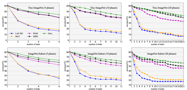
Figure 4: Results on Tiny-ImageNet and ImageNet-Subset for different numbers of tasks. Our method outperforms others, especially on longer task sequences (i.e. more, but smaller, tasks).

Dataset	Tiny-ImageNet			ImageNet-Subset
Method	5 tasks	10 tasks	20 tasks	5 tasks	10 tasks	20 tasks
LwF_MC	17.12	12.33	8.75	24.10	20.01	17.42
MUC	17.98	14.54	12.70	27.89	22.65	20.12
PASS	41.58	39.28	32.78	52.61	50.44	46.07
SSRE	41.67	39.89	39.76	58.46	57.51	50.05
ROSS	44.13	43.86	43.55	63.14	60.94	57.60

Table 3: Top-1 accuracy on all learned classes after the last task.

We report the comparative performance on CIFAR-100 in Table 1. ROSS outperforms all data-free approaches. For exemplar-based methods like iCaRL [29], EEIL [2], and LUCIR [13], our method still has significantly better performance. On longer sequences (i.e. 10 and 20 tasks), our method significantly reduces forgetting when learning new classes compared with other DFCIL methods. ROSS outperforms the best method SSRE by about 3% accuracy on the last task. The performance improvement can be also observed in terms of average forgetting.

As we can see in Table 3 and Figure 4 for Tiny-ImageNet and ImageNet-Subset, although our method has the similar top-1 accuracy on the first task in Figure 4, it has better performance at most intermediate tasks and also the final one. For longer sequences in Figure 4, the gap between our method and the best baseline is largely consistent, showing the effectiveness of our method at relieving forgetting. The performance gain in Table 3 is larger on Tiny-ImageNet and ImageNet-Subset compared to CIFAR100, and this demonstrates the generality of our method to datasets with larger images and object scales. It is worth mentioning that ROSS also produces results with smaller variance. We believe this to be due to ROSS reducing saliency drift to background regions, which may include random noise.

Plug-and-play with other DFCIL methods. Some existing DFCIL methods, for example PASS [42], IL2A [41] and SSRE [43], focus on reducing forgetting via embedding regularization. Considering the importance of saliency to image classification, it is natural consider whether ROSS can be integrated into these methods. The results in Table 2 show the performance gain brought by integrating ROSS with these methods. Adding ROSS doubles the performance for MUC in many cases and significantly improves IL2A and PASS. When we incorporate it into the best baseline SSRE, it yields a consistent gain of about 3%. These results clearly show that ROSS, by specifically mitigating saliency drift, is complementary to other methods in relieving forgetting in DFCIL. They additionally demonstrate the significance of saliency drift as a cause of catastrophic forgetting in DFCIL.

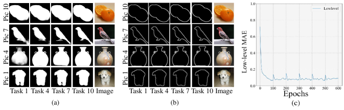
Figure 5: Visualization of the saliency (a) and boundary (b) maps from our student encoder-decoder network with original images from different tasks at different stages of incremental learning. Our method also produces stable low-level results while reducing forgetting in classification. (c) The MAE loss of low-level tasks between the student and teacher network across tasks.

Task 1
Task 3
Task 5
	Stage 0	Stage 1	Stage 2	Stage 3	Stage 4

(a)

Ours
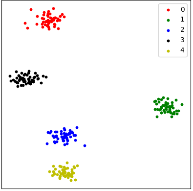
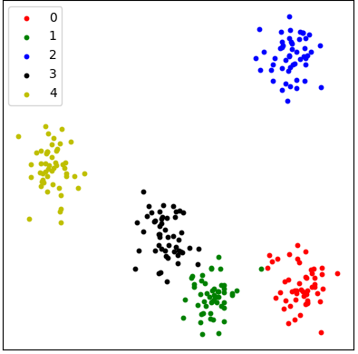
Baseline
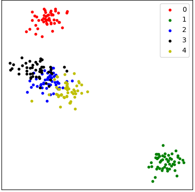
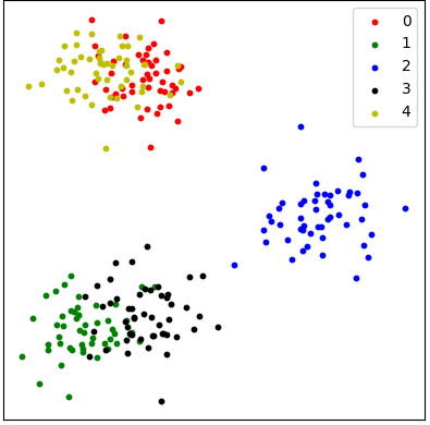
	Base task	Last task

(b)

Figure 6: Visualization of saliency across tasks at different stages as shown in (a). Stage 0 denotes the image-level saliency map. Some saliency drift at later tasks are recovered through multiple stages. Dilated boundary supervision also shrinks the saliency map at deeper stages, increasing their robustness. (b) Visualization of the embedding $F_{\phi}(x)$ with and without ROSS. Compared to the baseline, our method preserves more discriminative representations between classes from one task and between different tasks.

4.3 Additional Analysis

In this section we take a deeper look at the method we propose. If not specified, the results are produced using ROSS integrated into SSRE [43].

Ablation Study. To assess each component ROSS, we performed a set of ablations using the 10-task setting on CIFAR-100 (see Table 4). We do ablations on both PASS [42] and SSRE [43]. Low-level multi-task supervision is crucial and improve by 2.2% and 1.2% for PASS and SSRE, respectively. Dilated boundary supervison further boosts the performance by about 1-2 points. Saliency noise injection is also helpful for both methods and it improves by 1.5% points for PASS. In total, ROSS improves baselines by 5.5% and 2.9% points, respectively. Note that SSRE is the previous state-of-the-art method and our method outperforms it by a large margin.

Method & Tasks	LM	DBS	SNI	Accuracy
Baseline (PASS)				49.0
Variants	✓			51.2
	✓	✓		53.0
	✓	✓	✓	54.5
Baseline (SSRE)				55.0
Variants	✓			56.2
	✓	✓		57.3
	✓	✓	✓	57.9

Table 4: Ablative experiments on each component of our proposed method. Experiments are on CIFAR-100 in the 10 task setting and we report the top-1 accuracy in %, demonstrating the effect of integrating ROSS into PASS and SSRE. We use DBS, LM, SNI to denote the three components of ROSS: dilated boundary supervision, low-level multi-task supervision, and saliency noise injection.

Low-level multi-task. To analyze the effect of our proposed low-level saliency supervision, we performed experiments on ImageNet-Subset in the 5 and 10 task settings. We first plot the loss across tasks in Figure 5(c). After learning to predict boundary and saliency maps in the first task, the network maintains good performance for the rest of the 5 task sequence. This shows that the low-level tasks are stable during continual learning. Furthermore, we visualize the results of saliency and boundary map prediction during incremental learning in Figure 5(a-b). We give some examples of predicted boundary and saliency maps after learning different tasks. Although CIL involves samples of different classes, we see that the low-level outputs are relatively stable and class-agnostic. Since the model is able to stably predict these low-level features across tasks, it therefore can preserve useful prior knowledge for continual learning.

Saliency denoising across stages. To show the effect of saliency denoising, we look at the 5-task setting on ImageNet-Subset. We visualize a sample and its saliency at different training phases and encoder stages in Figure LABEL:fig:pa1. With the help of the denoising process, the encoder is able to mitigate intermediate saliency drift and maintain accurate attention. When testing on old samples, the network reduces the saliency drift and focuses on important regions.

Discriminative embeddings over different classes. Since our method helps the model focus on the foreground, more class-specific pixels are used to computing embeddings. This makes them more discriminative with less distracting background information. In Figure LABEL:fig:pc1 we use t-SNE to visualize embeddings of five initial classes after learning the base task and the last task in the 10-task setting on ImageNet-Subset in. At the base task, both Baseline (SSRE) and Ours (SSRE+ROSS) perform well. When visualizing after the last task, it is clear that ROSS can helps maintain discriminative features between tasks while the Baseline has overlapping embeddings.

5 Conclusions

In this paper we propose robust saliency guidance for DFCIL. The insight behind ROSS is to consider guiding the model to focus on salient regions with less drift. We show that robust saliency guidance is crucial to mitigate forgetting across tasks. Experiments demonstrate that ROSS is effective and surpasses the state-of-the-art. ROSS can be easily combined with other methods, leading to large performance gains over baselines. Qualitative results also show that low-level tasks are stable across different tasks, resulting in less catastrophic forgetting.

Figure 7: Visualization of some generated saliency noise maps.

Appendix A Further Ablation Studies

Ablation on student saliency methods.

To show the generalization of ROSS, we use several methods to compute student saliency maps and report the results in Table 5. Grad-CAM performs the best, although other methods yield performance gains, demonstrating the effectiveness of ROSS.

Method	5 Tasks	10 Tasks	20 Tasks
baseline (SSRE)	40.2	40.0	39.3
CAM	41.2	40.7	40.4
SmoothGrad	42.1	41.0	40.4
Grad-CAM	44.1	43.9	43.5

Table 5: Ablation on methods for generating student saliency maps on Tiny-Imagenet.

Ablation on low-level teacher maps.

In the manuscript we use CSNet [5] to compute all the teacher saliency and boundary maps because it is very lightweight. Compared to our main model, the teacher model has fewer than 1% parameters and requires 1.5% of the FLOPs (as shown in Table 6). Note that we compute all low-level maps offline before new tasks, and so the extra FLOPs should be amortized over the number of epochs. Therefore, the additional FLOPs required by the teacher model is only about 0.015% of the main model, which is negligible in practice.

To show the effectiveness of ROSS, we perform an ablation on the low-level teacher maps. We replace them with the Grad-CAM generated from a ResNet-152 network. To avoid information leakage, ResNet-152 was trained from scratch. Before each new task, we first train it only on task data and use the Grad-CAM output to supervise saliency in our incremental model. From Table 7 we see that ROSS still outperforms other methods. Moreover, ROSS is applicable to other teacher models for predicting saliency maps, (e.g. DFI [21] or PoolNet [22]) with more parameters, and produces even better performance with larger networks.

Model	Parameter(M)	FLOPS(G)
Ours	17.9	0.78
Teacher model	0.0941	0.012

Table 6: Parameters and FLOPs of the teacher model. FLOPs are computed using $3\times 32\times 32$ images.

Low-level source (Method)	Accuracy (%)
PASS	39.3
SSRE	40.0
ResNet152 (Ours)	42.1
CSNet (Ours)	43.9
PoolNet (Ours)	44.2
DFI (Ours)	44.4

Table 7: Ablation on low-level teacher saliency maps on Tiny-ImageNet with 10 tasks.

Ablation on student architecture and teacher pretraining.

We select PASS [42] as our baseline method to apply ROSS to (as shown in Table 8 and Table 9). Experiments in these two tables are conducted on ImageNet-Subset with 5 tasks. Since some methods use ImageNet pretrained weights for better saliency map estimation, we train CSNet [5] from scratch on the dataset (with and without pretraining) for salient object detection [35, 19, 36]. This allows us to verify that no information leakage happens due to pretraining the saliency network on ImageNet. The teacher network without pretraining works almost as well as pretraining the saliency network on ImageNet. We also compare the number of parameters of different methods in Table 8. This shows that adding network capacity for PASS from ResNet-18 to ResNet-32 with more parameters only improves the performance marginally. Ours with ResNet-18 based on PASS achieves a significant gain surpassing SSRE which has more parameters.

Method	Parameter (M)	Accuracy (%)
PASS-Res18	14.5	50.4
PASS-Res32	21.7	51.2
SSRE-Res18	19.4	58.7
Ours-Res18	17.9	61.5

Table 8: Comparison of different student network architectures. Method-Res18 denotes applying Method with ResNet18 as its backbone.

Method	Accuracy (%)
No pretraining	61.5
Pretrained teacher model	62.0

Table 9: Ablation on teacher network pretraining.

Appendix B More Details on Salience Noise Generation

For each ellipse there are 6 dimensions: the center coordinate $(x,y)$, the rotation angle $\alpha$, the mask weight $w$, and the major and minor axes $(a,b)$. $x$, $y$, $\alpha$ and $w$ are sampled from a uniform distribution over ranges: $x\in[0,H)$, $y\in[0,W)$, $\alpha\in[0,2\pi)$, $w\in[0,1]$. $H$ and $W$ denote the height and width of input images. To generate ellipses of appropriate size, we draw the major and minor axes from a Gaussian distribution with $\mu_{a}=\max(H,W)/2$, $\sigma_{a}=\max(H,W)/6$, $\mu_{b}=\min(H,W)/2$, $\sigma_{b}=\min(H,W)/6$. The sampled $a,b$ is clipped to$[0,max(H,W)/2]$ and $[0,min(H,W)/2]$, respectively. For each ellipse, we create a saliency map $S_{i}$. We repeat this random generation process 3-5 times and apply an element-wise max operation on the $S_{i}$ to obtain a single saliency map $S$. Then we crop and resize $S$ to the original image size, with crop size sampled from a uniform distribution in $[\min(H,W)/2,\min(H,W)]$, introducing center-aware saliency noise to the network for training. Finally, we apply a Gaussian blur on $S$ to better simulate a realistic saliency map. The kernel size for Gaussian blurring is the closest odd integer to $\min(H,W)/20$. For each encoder feature map, 10% of randomly selected channels are directly masked with $S$, where each selected channel will have an independent $S$. We visualize several generated samples in Figure 7.

References

- [1] Eden Belouadah, Adrian Popescu, and Ioannis Kanellos. A comprehensive study of class incremental learning algorithms for visual tasks. Neural Networks, 135:38–54, 2021.
- [2] Francisco M Castro, Manuel J Marín-Jiménez, Nicolás Guil, Cordelia Schmid, and Karteek Alahari. End-to-end incremental learning. In Proceedings of the European conference on computer vision (ECCV), pages 233–248, 2018.
- [3] Arslan Chaudhry, Marc’Aurelio Ranzato, Marcus Rohrbach, and Mohamed Elhoseiny. Efficient lifelong learning with a-gem. In ICLR, 2019.
- [4] Hanting Chen, Yunhe Wang, Chang Xu, Zhaohui Yang, Chuanjian Liu, Boxin Shi, Chunjing Xu, Chao Xu, and Qi Tian. Data-free learning of student networks. In Proceedings of the IEEE/CVF International Conference on Computer Vision, pages 3514–3522, 2019.
- [5] Ming-Ming Cheng, Shanghua Gao, Ali Borji, Yong-Qiang Tan, Zheng Lin, and Meng Wang. A highly efficient model to study the semantics of salient object detection. IEEE Transactions on Pattern Analysis and Machine Intelligence, 2021.
- [6] Matthias Delange, Rahaf Aljundi, Marc Masana, Sarah Parisot, Xu Jia, Ales Leonardis, Greg Slabaugh, and Tinne Tuytelaars. A continual learning survey: Defying forgetting in classification tasks. IEEE Transactions on Pattern Analysis and Machine Intelligence, 2021.
- [7] Jia Deng, Wei Dong, Richard Socher, Li-Jia Li, Kai Li, and Li Fei-Fei. Imagenet: A large-scale hierarchical image database. In 2009 IEEE conference on computer vision and pattern recognition, pages 248–255. Ieee, 2009.
- [8] Prithviraj Dhar, Rajat Vikram Singh, Kuan-Chuan Peng, Ziyan Wu, and Rama Chellappa. Learning without memorizing. In Proceedings of the IEEE/CVF conference on computer vision and pattern recognition, pages 5138–5146, 2019.
- [9] Arthur Douillard, Matthieu Cord, Charles Ollion, Thomas Robert, and Eduardo Valle. Podnet: Pooled outputs distillation for small-tasks incremental learning. In ECCV, 2020.
- [10] Sayna Ebrahimi, Suzanne Petryk, Akash Gokul, William Gan, Joseph E. Gonzalez, Marcus Rohrbach, and trevor darrell. Remembering for the right reasons: Explanations reduce catastrophic forgetting. In International Conference on Learning Representations, 2021.
- [11] Ian J Goodfellow, Mehdi Mirza, Da Xiao, Aaron Courville, and Yoshua Bengio. An empirical investigation of catastrophic forgetting in gradient-based neural networks. arXiv preprint arXiv:1312.6211, 2013.
- [12] Kaiming He, Xiangyu Zhang, Shaoqing Ren, and Jian Sun. Deep residual learning for image recognition. In CVPR, 2016.
- [13] Saihui Hou, Xinyu Pan, Chen Change Loy, Zilei Wang, and Dahua Lin. Learning a unified classifier incrementally via rebalancing. In Proceedings of the IEEE/CVF Conference on Computer Vision and Pattern Recognition, pages 831–839, 2019.
- [14] Aya Abdelsalam Ismail, Hector Corrada Bravo, and Soheil Feizi. Improving deep learning interpretability by saliency guided training. Advances in Neural Information Processing Systems, 34, 2021.
- [15] James Kirkpatrick, Razvan Pascanu, Neil Rabinowitz, Joel Veness, Guillaume Desjardins, Andrei A Rusu, Kieran Milan, John Quan, Tiago Ramalho, Agnieszka Grabska-Barwinska, et al. Overcoming catastrophic forgetting in neural networks. Proceedings of the national academy of sciences, 114(13):3521–3526, 2017.
- [16] Alex Krizhevsky, Geoffrey Hinton, et al. Learning multiple layers of features from tiny images. 2009.
- [17] Ya Le and Xuan Yang. Tiny imagenet visual recognition challenge. CS 231N, 7(7):3, 2015.
- [18] Xiangtai Li, Ansheng You, Zhen Zhu, Houlong Zhao, Maoke Yang, Kuiyuan Yang, and Yunhai Tong. Semantic flow for fast and accurate scene parsing. In ECCV, 2020.
- [19] Yin Li, Xiaodi Hou, Christof Koch, James M Rehg, and Alan L Yuille. The secrets of salient object segmentation. In Proceedings of the IEEE conference on computer vision and pattern recognition, pages 280–287, 2014.
- [20] Zhizhong Li and Derek Hoiem. Learning without forgetting. In 14th European Conference on Computer Vision, ECCV 2016, pages 614–629. Springer, 2016.
- [21] Jiang-Jiang Liu, Qibin Hou, and Ming-Ming Cheng. Dynamic feature integration for simultaneous detection of salient object, edge and skeleton. IEEE Transactions on Image Processing, pages 1–15, 2020.
- [22] Jiang-Jiang Liu, Qibin Hou, Ming-Ming Cheng, Jiashi Feng, and Jianmin Jiang. A simple pooling-based design for real-time salient object detection. In Proceedings of the IEEE/CVF conference on computer vision and pattern recognition, pages 3917–3926, 2019.
- [23] Yu Liu, Sarah Parisot, Gregory Slabaugh, Xu Jia, Ales Leonardis, and Tinne Tuytelaars. More classifiers, less forgetting: A generic multi-classifier paradigm for incremental learning. In European Conference on Computer Vision, pages 699–716. Springer, 2020.
- [24] David Lopez-Paz and Marc’Aurelio Ranzato. Gradient episodic memory for continual learning. Advances in neural information processing systems, 30, 2017.
- [25] Arun Mallya and Svetlana Lazebnik. Packnet: Adding multiple tasks to a single network by iterative pruning. In Proceedings of the IEEE conference on Computer Vision and Pattern Recognition, pages 7765–7773, 2018.
- [26] Marc Masana, Xialei Liu, Bartlomiej Twardowski, Mikel Menta, Andrew D Bagdanov, and Joost van de Weijer. Class-incremental learning: survey and performance evaluation on image classification. arXiv preprint arXiv:2010.15277, 2020.
- [27] Michael McCloskey and Neal J Cohen. Catastrophic interference in connectionist networks: The sequential learning problem. In Psychology of learning and motivation, volume 24, pages 109–165. Elsevier, 1989.
- [28] Quang Pham, Chenghao Liu, and Steven Hoi. Dualnet: Continual learning, fast and slow. Advances in Neural Information Processing Systems, 34, 2021.
- [29] Sylvestre-Alvise Rebuffi, Alexander Kolesnikov, Georg Sperl, and Christoph H Lampert. icarl: Incremental classifier and representation learning. In Proceedings of the IEEE conference on Computer Vision and Pattern Recognition, pages 2001–2010, 2017.
- [30] Matthew Riemer, Ignacio Cases, Robert Ajemian, Miao Liu, Irina Rish, Yuhai Tu, and Gerald Tesauro. Learning to learn without forgetting by maximizing transfer and minimizing interference. In In International Conference on Learning Representations (ICLR), 2019.
- [31] Ramprasaath R Selvaraju, Michael Cogswell, Abhishek Das, Ramakrishna Vedantam, Devi Parikh, and Dhruv Batra. Grad-cam: Visual explanations from deep networks via gradient-based localization. In Proceedings of the IEEE international conference on computer vision, pages 618–626, 2017.
- [32] James Smith, Yen-Chang Hsu, Jonathan Balloch, Yilin Shen, Hongxia Jin, and Zsolt Kira. Always be dreaming: A new approach for data-free class-incremental learning. In Proceedings of the IEEE/CVF International Conference on Computer Vision, pages 9374–9384, 2021.
- [33] Yue Wu, Yinpeng Chen, Lijuan Wang, Yuancheng Ye, Zicheng Liu, Yandong Guo, and Yun Fu. Large scale incremental learning. In Proceedings of the IEEE/CVF Conference on Computer Vision and Pattern Recognition, pages 374–382, 2019.
- [34] Ju Xu and Zhanxing Zhu. Reinforced continual learning. Advances in Neural Information Processing Systems, 31, 2018.
- [35] Qiong Yan, Li Xu, Jianping Shi, and Jiaya Jia. Hierarchical saliency detection. In Proceedings of the IEEE conference on computer vision and pattern recognition, pages 1155–1162, 2013.
- [36] Chuan Yang, Lihe Zhang, Huchuan Lu, Xiang Ruan, and Ming-Hsuan Yang. Saliency detection via graph-based manifold ranking. In Proceedings of the IEEE conference on computer vision and pattern recognition, pages 3166–3173, 2013.
- [37] Hongxu Yin, Pavlo Molchanov, Jose M Alvarez, Zhizhong Li, Arun Mallya, Derek Hoiem, Niraj K Jha, and Jan Kautz. Dreaming to distill: Data-free knowledge transfer via deepinversion. In Proceedings of the IEEE/CVF Conference on Computer Vision and Pattern Recognition, pages 8715–8724, 2020.
- [38] Lu Yu, Bartlomiej Twardowski, Xialei Liu, Luis Herranz, Kai Wang, Yongmei Cheng, Shangling Jui, and Joost van de Weijer. Semantic drift compensation for class-incremental learning. In Proceedings of the IEEE/CVF Conference on Computer Vision and Pattern Recognition, pages 6982–6991, 2020.
- [39] Junting Zhang, Jie Zhang, Shalini Ghosh, Dawei Li, Serafettin Tasci, Larry Heck, Heming Zhang, and C-C Jay Kuo. Class-incremental learning via deep model consolidation. In Proceedings of the IEEE/CVF Winter Conference on Applications of Computer Vision, pages 1131–1140, 2020.
- [40] Jia-Xing Zhao, Jiang-Jiang Liu, Deng-Ping Fan, Yang Cao, Jufeng Yang, and Ming-Ming Cheng. Egnet: Edge guidance network for salient object detection. In Proceedings of the IEEE/CVF international conference on computer vision, pages 8779–8788, 2019.
- [41] Fei Zhu, Zhen Cheng, Xu-yao Zhang, and Cheng-lin Liu. Class-incremental learning via dual augmentation. Advances in Neural Information Processing Systems, 34, 2021.
- [42] Fei Zhu, Xu-Yao Zhang, Chuang Wang, Fei Yin, and Cheng-Lin Liu. Prototype augmentation and self-supervision for incremental learning. In Proceedings of the IEEE/CVF Conference on Computer Vision and Pattern Recognition, pages 5871–5880, 2021.
- [43] Kai Zhu, Wei Zhai, Yang Cao, Jiebo Luo, and Zheng-Jun Zha. Self-sustaining representation expansion for non-exemplar class-incremental learning. In Proceedings of the IEEE/CVF Conference on Computer Vision and Pattern Recognition, pages 9296–9305, 2022.